Spaces of ranked tree-child networks

Abstract.

Ranked tree-child networks are a recently introduced class of rooted phylogenetic networks in which the evolutionary events represented by the network are ordered so as to respect the flow of time. This class includes the well-studied ranked phylogenetic trees (also known as ranked genealogies). An important problem in phylogenetic analysis is to define distances between phylogenetic trees and networks in order to systematically compare them. Various distances have been defined on ranked binary phylogenetic trees, but very little is known about comparing ranked tree-child networks. In this paper, we introduce an approach to compare binary ranked tree-child networks on the same leaf set that is based on a new encoding of such networks that is given in terms of a certain partially ordered set. This allows us to define two new spaces of ranked binary tree-child networks. The first space can be considered as a generalization of the recently introduced space of ranked binary phylogenetic trees whose distance is defined in terms of ranked nearest neighbor interchange moves. The second space is a continuous space that captures all equidistant tree-child networks and generalizes the space of ultrametric trees. In particular, we show that this continuous space is a so-called CAT(0)-orthant space which, for example, implies that the distance between two equidistant tree-child networks can be efficiently computed.

1. Introduction

Rooted phylogenetic networks are essentially directed acyclic graphs, whose leaf sets correspond to a set of species. They are commonly used to represent evolutionary histories in which reticulate events have occurred due to processes such as hybridization and lateral gene transfer. Various classes of rooted phylogenetic networks have been defined, including the extensively studied class of so-called tree child networks introduced by Cardona et al., (2008) (see e.g. Kong et al., (2022) for a review). Recently, the class of (binary) ranked tree child networks (RTCNs) was introduced by Bienvenu et al., (2022), which have been further studied by Caraceni et al., (2022) and Fuchs et al., (2024). As their name suggests, these are a special type of tree-child network that are endowed with additional information which allows the evolutionary events represented by the network to be arranged consistently along a time line. RTCNs generalize ranked phylogenetic trees (also called ranked genealogies), structures that can be used to study evolutionary dynamics (see e.g. Kim et al., (2020) and the references therein).

Informally (see Section 2 and Section 6 for full definitions), a binary RTCN is a binary rooted phylogenetic network with leaf set $X$ having the following additional restrictions: (i) every vertex that is not a leaf must be the tail of some arc whose head has no other in-coming arcs and (ii) vertices are assigned ranks from the set $\{1,\dots,|X|\}$ such that the tail of an arc never has a smaller rank than the head. In Figure 1(a) we give an example of a binary RTCN. In addition, by assigning non-negative weights to the arcs of an RTCN that are consistent with the ranks of the vertices (in particular, vertices having the same rank also have the same distance from the root) we obtain an equidistant tree-child network (ETCN). An example of an ETCN is given in Figure 1(b).

Figure 1. (a) A binary RTCN on the set $X=\{a,b,c,d,e\}$. Each dotted horizontal line corresponds to vertices that have the same rank. (b) An ETCN on $X$ obtained by assigning suitable weights to the arcs of the RTCN in (a).

Comparing phylogenetic trees and networks is an important problem in phylogenetics which has been studied for some time, and various distances have been defined on trees and networks (see e.g. Cardona et al., (2008); Huber et al., (2016); Janssen et al., (2018); Kuhner and Yamato, (2015); Nakhleh, (2009); Pons et al., (2019); Smith, (2022)), including ranked phylogenetic trees (Kim et al.,, 2020). Thus it is a natural question to ask for ways to compare RTCNs and ETCNs. In this paper, we shall present some new distances for such networks and consider some properties of the resulting spaces. We define our distances by introducing a way to encode binary RTCNs on a fixed leaf set $X$ in terms of a certain partially ordered set (or poset). As we shall see in Section 3, as well as encoding binary RTCNs, this poset has some attractive mathematical properties, including the fact that it generalizes the well-known poset of partitions of the set $X$, a poset that captures the set of all binary ranked trees with leaf set $X$ (see e.g. Huber et al., (2024, Sec. 4.2)).

Using our new encoding, in Section 4 we provide a generalization of the Robinson-Foulds distance on rooted phylogenetic trees, and also define a generalization of the ranked nearest neighbor interchange (rNNI) distance on binary ranked trees introduced by Gavryushkin et al., (2018) to all binary RTCNs, thus providing a way to compare binary RTCNs. In addition, in Section 6 we define a continuous metric space of ETCNs whose definition relies on some special properties of the poset mentioned above. More specifically, we show that this space is a so-called CAT(0)-orthant space, which implies that the distance between any two ETCNs can be computed efficiently. Note that Billera et al., (2001) presented a similar approach to compare unrooted edge-weighted phylogenetic trees, and that our space of ETCNs generalizes the more recently introduced spaces of ultrametric trees (Gavryushkin and Drummond,, 2016) and equidistant cactuses (Huber et al.,, 2024).

We now describe the contents of the rest of this paper. After formally defining binary RTCNs in Section 2, we show how binary RTCNs with a fixed leaf set correspond to maximal chains of certain cluster systems (Section 3). Then we introduce the poset capturing all binary RTCNs, present our generalization of rNNIs and show that the discrete space of all binary RTCNs is connected under these more general rNNIs (Section 4). Next we describe how our poset also systematically captures certain non-binary RTCNs (Section 5) and use this to describe our CAT(0)-orthant space of ETCNs (Section 6). We conclude mentioning some possible directions for future work (Section 7).

2. Binary ranked tree-child networks

In this section, we formally define the basic type of phylogenetic network that we consider in this paper. For the rest of this paper, $X$ will be a finite non-empty set with $n=|X|\geq 2$, which can be thought of as a set of species or taxa.

A directed graph $G=(V,E)$ consists of a finite, non-empty set $V$ of vertices and a set $E\subseteq V\times V$ of directed edges or arcs. We write $(u,v)$ for an arc that is directed from vertex $u$, the tail of the arc, to vertex $v$, the head of the arc. For a vertex $u$, the out-degree of $u$ is the number of arcs that have $u$ as its tail and the in-degree of $u$ is the number of arcs that have $u$ as its head. A leaf is a vertex of out-degree 0. A directed path in $G$ from vertex $s$ to vertex $t$ is a sequence $s=v_{1},v_{2},\dots,v_{k}=t$ of $k\geq 1$ pairwise distinct vertices with $(v_{i},v_{i+1})\in E$ for all $1\leq i\leq k-1$. Note that we allow $k=1$, which then implies that $s=t$. A directed graph $G$ is acyclic if it does not contain a directed path from some vertex $s$ to some vertex $t$ such that $(t,s)$ is an arc in $G$ (which would then form a directed cycle in $G$).

A rooted phylogenetic network $\mathcal{N}=(V,E,\rho)$ on $X$ is a directed acyclic graph $G=(V,E)$ with leaf set $X$ and a unique vertex $\rho$ of in-degree 0, called the root of $\mathcal{N}$. A vertex of $\mathcal{N}$ that is not a leaf is called an interior vertex. A vertex of $\mathcal{N}$ with in-degree at least 2 is a hybrid vertex. Any vertex of $\mathcal{N}$ that is not a hybrid vertex is a tree vertex. A rooted phylogenetic network is binary if the root has out-degree 2 and every other interior vertex either has in-degree 1 and out-degree 2 or in-degree 2 and out-degree 1.

We now define what we mean by a binary ranked tree-child network (RTCN) following (Bienvenu et al.,, 2022, Sec. 2.1), which describes how any such network on a fixed set $X$ can be obtained using a process involving $n$ steps:

• Step 1: For each $x\in X$ an arc with head $x$ is created. The tails of these arcs are pairwise distinct and form a set of $n$ vertices with in-degree 0 (see Figure 2(a)).

• Step $i$ $(2\leq i\leq n-1)$: Precisely one of the following modifications to the network obtained in Step $i-1$ is performed:

  • Two vertices with in-degree 0 are selected. These two vertices are identified as a single vertex $u$ with out-degree 2. Then a new arc with head $u$ and a new vertex as its tail is added (see Figure 2(b)).

  • Three vertices $u$, $v$ and $w$ with in-degree 0 are selected. Then arcs $(u,v)$ and $(w,v)$ are added, making $v$ a hybrid vertex. Then two new arcs with head $u$ and $w$, respectively, and each with a new vertex as its tail are added (see Figure 2(c)).

  After performing Step $i$ we have a network that has $n-i+1$ vertices with in-degree 0.

• Step $n$: The result of Step $n-1$ is a network with precisely two vertices with in-degree 0. These two vertices are identified as a single vertex which then forms the root $\rho$ of the resulting binary RTCN. This finishes the process of generating a binary RTCN (see Figure 2(d)).

Figure 2. An example of the process that generates a binary RTCN on $X=\{a,b,c,d\}$. (a) The result of Step 1. (b) The result of performing (1) in Step 2. (c) The result of performing (2) in Step 3. (d) The resulting binary RTCN after Step $n=4$. Vertices of rank $i$ are drawn on the dotted horizontal line numbered $i$ $(1\leq i\leq 4)$.

All different binary RTCNs on a fixed set $X$ arise through the choice of performing either (1) or (2) in Steps $2,\dots,n-1$ and, subsequently, the choice of either the two vertices used in (1) or the three vertices used on (2). Note that in (2) the role of vertex $v$ is different from the roles of vertices $u$ and $w$. So, more precisely, performing (2) also involves a choice which of the three selected vertices plays the role of the vertex that becomes a hybrid vertex. If (2) is never performed in any of the Steps $2,\dots,n-2$ the network only contains tree vertices and is called a binary ranked tree.

Each vertex $q$ in a binary RTCN $\mathcal{N}=(V,E,\rho)$ on $X$ has a rank from the set $\{1,\dots,n\}$ associated with it that is denoted by $\text{rank}(q)$. More precisely (see Figure 2(d)), we have

• $\text{rank}(x)=1$ for all $x\in X$,

• $\text{rank}(u)=i$ when (1) is performed in Step $i$ $(2\leq i\leq n-1)$,

• $\text{rank}(u)=\text{rank}(v)=\text{rank}(w)=i$ when (2) is performed in Step $i$ $(2\leq i\leq n-1)$, and

• $\text{rank}(\rho)=n$.

These ranks correspond to an ordering of the biological events (speciation or hybridization) that led from the common ancestor at the root of the network to the elements in $X$ at the leaves. The term tree-child refers to the fact that in the networks generated by the process described above every interior vertex is the tail of an arc whose head is a tree-vertex. Note that tree-child networks without ranked vertices were introduced by Cardona et al., (2008) and remain an active area of research (see e.g. Cardona et al., (2019); Cardona and Zhang, (2020); Fuchs et al., (2021)).

3. Encoding binary ranked tree-child networks

In this section, we present a way to encode binary RTCNs, that is, a way to describe binary RTCNs in such a way that two RTCNs are the same if and only if they have the same description. The encoding itself is a straight-forward translation of the process described in Section 2 for generating a binary RTCN into the language of collections of subsets of $X$. As we will see later on, this encoding is very helpful for proving our results about RTCNs.

To formally describe the encoding, we first give some more definitions. A cluster on $X$ is a non-empty subset of $X$. A cluster system on $X$ is a non-empty collection of clusters on $X$. Given a rooted phylogenetic network $\mathcal{N}=(V,E,\rho)$ on $X$, to each each vertex $v\in V$, we associate the cluster $C_{v}$ on $X$ that consists of all those $x\in X$ for which there exists a directed path in $\mathcal{N}$ from $v$ to $x$. The clusters given in this way are sometimes called the hard-wired clusters of the network.

Each step $i$ $(1\leq i\leq n)$ in the process described in Section 2 can now be captured by a cluster system $\mathcal{C}_{i}$ on $X$ as follows:

• Step 1: $\mathcal{C}_{1}=\{\{x\}:x\in X\}$. Each cluster in $\mathcal{C}_{1}$ consists of a single element and represents a leaf in the resulting network.

• Step $i$ $(2\leq i\leq n-1)$: We already have the cluster system $\mathcal{C}_{i-1}$ which consists of the clusters $C_{v}$ obtained from those vertices $v$ that are the head of an arc whose tail has in-degree 0 at the end of Step $i-1$.

  • If (1) is performed in Step $i$ there must exist clusters $A$ and $B$ in $\mathcal{C}_{i-1}$ such that $C_{u}=A\cup B$. Then we put $\mathcal{C}_{i}=(\mathcal{C}_{i-1}-\{A,B\})\cup\{C_{u}\}$.

  • If (2) is performed in Step $i$ there must exist clusters $A$, $B$ and $C$ in $\mathcal{C}_{i-1}$ such that $C_{u}=A\cup B$ and $C_{w}=B\cup C$. Then we put $\mathcal{C}_{i}=(\mathcal{C}_{i-1}-\{A,B,C\})\cup\{C_{u},C_{w}\}$.

  The cluster system $\mathcal{C}_{i}$ consists of $n-i+1$ clusters.

• Step $n$: The cluster system $\mathcal{C}_{n-1}$ consists of two clusters $A$ and $B$ such that $C_{\rho}=A\cup B=X$. We put $\mathcal{C}_{n}=(\mathcal{C}_{n-1}-\{A,B\})\cup\{C_{\rho}\}=\{X\}$.

To illustrate this definition, consider again the example of generating a binary RTCN on $X=\{a,b,c,d\}$ in Figure 2. Then we obtain the following cluster systems:

$$\mathcal{C}_{1} =\{\{a\},\{b\},\{c\},\{d\}\},$$

$$\mathcal{C}_{2} =(\mathcal{C}_{1}-\{\{a\},\{b\}\})\cup\{\{a,b\}\}=\{\{a,b\},\{c\},\{d\}\},$$

$$\mathcal{C}_{3} =(\mathcal{C}_{2}-\{\{a,b\},\{c\},\{d\}\})\cup\{\{a,b,c\},\{c,d\}\}=\{\{a,b,c\},\{c,d\}\},\mbox{ and }$$

$$\mathcal{C}_{4} =(\mathcal{C}_{3}-\{\{a,b,c\},\{c,d\}\})\cup\{\{a,b,c,d\}\}=\{\{a,b,c,d\}.\}$$

As also illustrated by this example, the cluster systems can easily be read from the resulting binary RTCN $\mathcal{N}=(V,E,\rho)$ on $X$: For $1\leq i<n$, we have

$$\mathcal{C}_{i}=\mathcal{C}_{i}(\mathcal{N})=\{C_{v}:\text{there exists an arc}\ (u,v)\in E\ \text{with rank}(u)>i\geq\text{rank}(v)\},$$

and $\mathcal{C}_{n}=\{C_{\rho}\}=\{X\}$.

To make more precise our way of encoding a binary RTCN $\mathcal{N}$ by the cluster systems

$$\mathcal{C}_{1}(\mathcal{N}),\dots,\mathcal{C}_{n}(\mathcal{N}),$$

we need a little bit more notation. Let $\mathcal{C}$ and $\mathcal{C}^{\prime}$ be cluster systems on $X$. We write:

• $\mathcal{C}\vdash_{(1)}\mathcal{C}^{\prime}$ if there exist two distinct clusters $A,B\in\mathcal{C}$ with $\mathcal{C}^{\prime}=(\mathcal{C}-\{A,B\})\cup\{A\cup B\}$ (see Figure 3(a)).

• $\mathcal{C}\vdash_{(2)}\mathcal{C}^{\prime}$ if there exist three pairwise distinct clusters $A,B,C\in\mathcal{C}$ with $\mathcal{C}^{\prime}=(\mathcal{C}-\{A,B,C\})\cup\{A\cup B,B\cup C\}$ (see Figure 3(b)).

We will often use the simplified notation $\mathcal{C}\vdash\mathcal{C}^{\prime}$ if either $\mathcal{C}\vdash_{(1)}\mathcal{C}^{\prime}$ or $\mathcal{C}\vdash_{(2)}\mathcal{C}^{\prime}$ holds in case it is not relevant which of the two conditions holds. A maximal chain on $X$ is a sequence $\mathcal{C}_{1},\dots,\mathcal{C}_{n}$ of $n$ cluster systems on $X$ such that

$$\{\{x\}:x\in X\}=\mathcal{C}_{1}\vdash\mathcal{C}_{2}\vdash\dots\vdash\mathcal{C}_{n}=\{X\}.$$

Figure 3. The two operations (a) $\vdash_{(1)}$ and (b) $\vdash_{(2)}$ that can be applied to a cluster system and how they are related to the process of generating binary RTCNs.

Before we state the main result of this section, we establish a useful property of cluster systems in a maximal chain on $X$.

Lemma 3.1.

Let $\mathcal{C}_{1},\dots,\mathcal{C}_{n}$ be a maximal chain on $X$ and $1\leq i\leq n$. Then every cluster in $\mathcal{C}_{i}$ contains an element in $X$ that is not contained in any other cluster in $\mathcal{C}_{i}$.

Proof: We use induction on $i$. In the base case of the induction, $i=1$, we have $\mathcal{C}_{1}=\{\{x\}:x\in X\}$. Then, clearly, for all $x\in X$, the element $x$ is only contained in the cluster $\{x\}$.

Next consider the case $i>1$. By the definition of a maximal chain, we have $\mathcal{C}_{i-1}\vdash\mathcal{C}_{i}$. By induction, all clusters in $\mathcal{C}_{i-1}$ contain at least one element that is not contained in any other cluster in $\mathcal{C}_{i-1}$. But then, in view of the definition of $\vdash_{(1)}$ and $\vdash_{(2)}$, it follows that also all clusters in $\mathcal{C}_{i}$ contain at least one element that is not contained in any other cluster in $\mathcal{C}_{i}$, as required.  

We now present our encoding for binary RTCNs.

Theorem 3.2.

Binary RTCNs on $X$ are in bijective correspondence with maximal chains on $X$.

Proof: We have already seen that from every binary RTCN $\mathcal{N}$ on $X$ we obtain the maximal chain $\mathcal{C}_{1}(\mathcal{N}),\dots,\mathcal{C}_{n}(\mathcal{N})$ on $X$.

So, assume that $\mathcal{C}_{1},\dots,\mathcal{C}_{n}$ is a maximal chain on $X$. To obtain a binary RTCN $\mathcal{N}$ on $X$ with $\mathcal{C}_{i}=\mathcal{C}_{i}(\mathcal{N})$ we use the maximal chain to guide the process of generating $\mathcal{N}$ during Steps $i=2,\dots,n-1$:

• If $\mathcal{C}_{i-1}\vdash_{(1)}\mathcal{C}_{i}$ we perform (1).

• If $\mathcal{C}_{i-1}\vdash_{(2)}\mathcal{C}_{i}$ we perform (2).

It remains to show that the two vertices with in-degree 0 used when performing (1) and the three vertices with in-degree 0 used when performing (2), respectively, are uniquely determined by the maximal chain on $X$. But this follows immediately from the property of the cluster systems in a maximal chain on $X$ stated in Lemma 3.1, as this allows to uniquely determine the clusters involved in $\mathcal{C}_{i-1}\vdash\mathcal{C}_{i}$.  

The encoding established in Theorem 3.2 is useful because it allows us to systematically break any binary RTCN on $X$ down into building blocks (i.e. cluster systems), which gives a simple way to understand the relationship between two binary RTCNs. We remark that there are two interesting special instances of our encoding:

• Maximal chains $\mathcal{C}_{1},\dots,\mathcal{C}_{n}$ on $X$ such that $\mathcal{C}_{1}\vdash_{(1)}\mathcal{C}_{2}\vdash_{(1)}\dots\vdash_{(1)}\mathcal{C}_{n}$ are in bijective correspondence with binary ranked trees on $X$.

• Let $\vdash^{*}$ be the restricted variant of $\vdash$ defined by the additional requirement that

  • for $\mathcal{C}\vdash^{*}_{(1)}\mathcal{C}^{\prime}$ to hold we must have $A\cap B\neq\emptyset$ or $A\cap C=\emptyset$ for all $C\in\mathcal{C}-\{A\}$ or $B\cap C=\emptyset$ for all $C\in\mathcal{C}-\{B\}$, and

  • for $\mathcal{C}\vdash^{*}_{(2)}\mathcal{C}^{\prime}$ to hold we must have $A\cap D=\emptyset$ for all $D\in\mathcal{C}-\{A\}$, $B\cap D=\emptyset$ for all $D\in\mathcal{C}-\{B\}$ and $C\cap D=\emptyset$ for all $D\in\mathcal{C}-\{C\}$.

  Then maximal chains $\mathcal{C}_{1},\dots,\mathcal{C}_{n}$ on $X$ such that $\mathcal{C}_{1}\vdash^{*}\mathcal{C}_{2}\vdash^{*}\dots\vdash^{*}\mathcal{C}_{n}$ are in bijective correspondence with binary ranked cactuses on $X$, a proper subclass of binary RTCNs considered by Huber et al., (2024).

4. Nearest neighbor interchange moves for binary RTCNs

In this section we explain how to use our encoding of binary RTCNs by maximal chains of cluster systems to compare unweighted binary RTCNs. One simple way to do this is to define the distance between two such networks $\mathcal{N}$ and $\mathcal{N}^{\prime}$ to be

$$|\{\mathcal{C}_{1}(\mathcal{N}),\dots,\mathcal{C}_{n}(\mathcal{N})\}\triangle\{\mathcal{C}_{1}(\mathcal{N}^{\prime}),\dots,\mathcal{C}_{n}(\mathcal{N}^{\prime})\}|$$

where $\triangle$ denotes the symmetric difference of sets. The metric on binary RTCNs arising in this way can be thought of as a ranked analogue of the Robinson-Foulds distance on rooted trees (Robinson and Foulds,, 1981).

Figure 4. The two types of modifications on binary ranked trees allowed in an rNNI: (a) Swapping the ranks of vertices $u$ and $v$. (b) An actual nearest neighbor interchange.

A more sophisticated approach is to define an analogue of the well-known nearest neighbor interchange distance for rooted phylogenetic trees (Robinson,, 1971). This distance has already been generalized to binary ranked trees by Gavryushkin et al., (2018) as follows. First, define two types of modifications of a binary ranked tree on $X$ (called ranked nearest neighbor interchanges (rNNIs)):

• For two vertices $u$ and $v$ with $\text{rank}(u)=\text{rank}(v)+1$ and $(u,v)$ not an arc, the ranks of $u$ and $v$ are swapped without changing the topology of the tree (see Figure 4(a)).

• For two vertices $u$ and $v$ with $\text{rank}(u)=\text{rank}(v)+1$ and $(u,v)$ an arc, the topology of the tree is changed (see Figure 4(b)).

Then, Gavryushkin et al., (2018) established the following result:

Fact 4.1.

For any two binary ranked trees $\mathcal{T}$ and $\mathcal{T}^{\prime}$ on $X$ there exists a sequence of rNNIs that transform $\mathcal{T}$ into $\mathcal{T}^{\prime}$.

Interestingly, as pointed out in the supplementary material by Collienne et al., (2021), there is a concise and uniform way to describe an rNNI between two binary ranked trees $\mathcal{T}$ and $\mathcal{T}^{\prime}$ on $X$ using the corresponding maximal chains $\mathcal{C}_{1},\dots,\mathcal{C}_{n}$ and $\mathcal{C}^{\prime}_{1},\dots,\mathcal{C}^{\prime}_{n}$ on $X$: There exists $2\leq i\leq n-1$ such that $\mathcal{C}_{i}\neq\mathcal{C}^{\prime}_{i}$ and $\mathcal{C}_{j}=\mathcal{C}^{\prime}_{j}$ for all $j\neq i$. Less formally, there is an rNNI between $\mathcal{T}$ and $\mathcal{T}^{\prime}$ if the corresponding maximal chains differ in precisely one cluster system. For example, consider the two binary ranked trees $\mathcal{T}$ and $\mathcal{T}^{\prime}$ on $X=\{a,b,c,d,e\}$ in Figure 4(a). Looking at the corresponding maximal chains on $X$ we have:

$$\mathcal{C}_{1} =\{\{a\},\{b\},\{c\},\{d\},\{e\}\}=\mathcal{C}^{\prime}_{1}$$

$$\mathcal{C}_{2} =\{\{a,b\},\{c\},\{d\},\{e\}\}\neq\{\{a\},\{b\},\{c\},\{d,e\}\}=\mathcal{C}^{\prime}_{2}$$

$$\mathcal{C}_{3} =\{\{a,b\},\{c\},\{d,e\}\}=\mathcal{C}^{\prime}_{3}$$

$$\mathcal{C}_{4} =\{\{a,b,c\},\{d,e\}\}=\mathcal{C}^{\prime}_{4}$$

$$\mathcal{C}_{5} =\{\{a,b,c,d,e\}\}=\mathcal{C}^{\prime}_{5}$$

While the description of rNNIs in terms of the binary ranked trees is very intuitive, it is not obvious how to directly generalize this to binary RTCNs. However, as with ranked trees, the description in terms of maximal chains on $X$ immediately suggests a way to do this: We say that there is a ranked nearest neighbor interchange between two binary RTCNs $\mathcal{N}$ and $\mathcal{N}^{\prime}$ (both on $X$) if the corresponding maximal chains on $X$ differ in precisely one cluster system. We shall continue to use rNNI when referring to ranked nearest neighbor interchanges restricted to binary ranked trees as described above and will use rNNI^∗ when referring to this generalization. Figure 5 illustrates what happens to the corresponding RTCNs when we apply such rNNI^∗s.

Figure 5. Two consecutive rNNI^∗s that transform the binary RTCN $\mathcal{N}$ on $X=\{a,b,c,d,e,f\}$ through the intermediate binary RTCN $\mathcal{N}^{\prime}$ to the binary ranked tree $\mathcal{T}$.

We conclude this section by establishing that for any two binary RTCNs on $X$ there exists a sequence of rNNI^∗s that transforms one into the other. This implies that we can define a distance between any pair of binary RTCNs by taking the length of a shortest sequence of rNNI^∗s that transforms one of the networks to the other.

Theorem 4.2.

For any two binary RTCNs $\mathcal{N}_{1}$ and $\mathcal{N}_{2}$ on $X$ there exists a sequence of rNNI^∗s that transform $\mathcal{N}_{1}$ into $\mathcal{N}_{2}$.

Proof: Since every rNNI between two binary ranked trees on $X$ is also an rNNI^∗ between them when we view the binary ranked trees as binary RTCNs, it suffices, by Fact 4.1, to show that for any binary RTCN $\mathcal{N}$ on $X$ there exists a sequence of rNNI^∗s that transforms $\mathcal{N}$ into some binary ranked tree $\mathcal{T}$ on $X$ (Figure 5 gives an example of such a sequence of rNNI^∗s).

Let $\mathcal{C}_{1},\dots,\mathcal{C}_{n}$ be the maximal chain on $X$ that corresponds to $\mathcal{N}$ by Theorem 3.2. The proof is by induction on the number $\ell$ of those $1<j\leq n$ with $\mathcal{C}_{j-1}\vdash_{(2)}\mathcal{C}_{j}$. In the base case of the induction, $\ell=0$, $\mathcal{N}$ is itself a binary ranked tree.

So, assume that $\ell>0$. Let $i$ be the maximum of those $1<j\leq n$ with $\mathcal{C}_{j-1}\vdash_{(2)}\mathcal{C}_{j}$. By the definition of $\vdash_{(2)}$ there exist three pairwise distinct $A,B,C\in\mathcal{C}_{i-1}$ such that

$$\mathcal{C}_{i}=(\mathcal{C}_{i-1}-\{A,B,C\})\cup\{A\cup B,B\cup C\}.$$

By Lemma 3.1, we can select from each cluster in $\mathcal{C}_{i}$ an element that is unique to this cluster. Let $X^{\prime}\subseteq X$ be the resulting subset of selected elements. To give an example, for the binary RTCN $\mathcal{N}$ in Figure 5 we have $i=3$ and can select $X^{\prime}=\{a,c,d,f\}$.

By the maximality of $i$, we have $\mathcal{C}_{j-1}\vdash_{(1)}\mathcal{C}_{j}$ for all $j>i$. Thus, after restricting all clusters to $X^{\prime}$, the sequence $\mathcal{C}_{i},\dots,\mathcal{C}_{n}$ becomes a maximal chain on $X^{\prime}$ that only contains partitions of $X^{\prime}$. This maximal chain on $X^{\prime}$ corresponds, by Theorem 3.2, to a binary ranked tree $\mathcal{T}_{1}^{\prime}$ on $X^{\prime}$. In Figure 6 the binary ranked tree $\mathcal{T}_{1}^{\prime}$ resulting from the binary RTCN $\mathcal{N}$ in Figure 5 is shown.

Let $y$ be the element in $X^{\prime}$ selected from $A\cup B$ and let $z$ be the element in $X^{\prime}$ selected from $B\cup C$. Let $\mathcal{T}_{2}^{\prime}$ be a binary ranked tree on $X^{\prime}$ that contains a vertex $u$ with $\text{rank}(u)=2$ and the arcs $(u,y)$ and $(u,z)$. Clearly, such a binary ranked tree exists and, by Fact 4.1, there exists a sequence of rNNIs that transforms $\mathcal{T}_{1}^{\prime}$ into $\mathcal{T}_{2}^{\prime}$. In Figure 6, a suitable binary ranked tree $\mathcal{T}_{2}^{\prime}$ is shown that arises by applying a single rNNI to $\mathcal{T}_{1}^{\prime}$.

The sequence of rNNIs transforming $\mathcal{T}_{1}^{\prime}$ into $\mathcal{T}_{2}^{\prime}$ corresponds to a sequence of rNNI^∗s that transform $\mathcal{N}$ into a binary RTCN $\mathcal{N}^{\prime}$ such that all vertices of $\mathcal{N}$ with rank at most $i$ remain unchanged and only the vertices corresponding to the binary ranked tree $\mathcal{T}_{1}^{\prime}$ are involved. In Figure 5 the binary RTCN $\mathcal{N}^{\prime}$ resulting from the rNNI between the binary ranked trees $\mathcal{T}_{1}^{\prime}$ and $\mathcal{T}_{2}^{\prime}$ in Figure 6 is shown.

In preparation for the last step in the proof, we summarize the properties of the maximal chain on $X$ that corresponds to $\mathcal{N}^{\prime}$:

• $\mathcal{C}_{j}(\mathcal{N}^{\prime})=\mathcal{C}_{j}(\mathcal{N})$ for all $1\leq j\leq i$

• $\mathcal{C}_{j-1}(\mathcal{N}^{\prime})\vdash_{(1)}\mathcal{C}_{j}(\mathcal{N}^{\prime})$ for all $i<j\leq n$

• $\mathcal{C}_{i+1}(\mathcal{N}^{\prime})=(\mathcal{C}_{i}(\mathcal{N}^{\prime})-\{A\cup B,B\cup C\})\cup\{A\cup B\cup C\}$

Now we perform the following rNNI^∗ on $\mathcal{N}^{\prime}$: We replace the cluster system $\mathcal{C}_{i}=\mathcal{C}_{i}(\mathcal{N}^{\prime})$ by the cluster system

$$\mathcal{C}_{i}^{\prime\prime}=(\mathcal{C}_{i-1}(\mathcal{N}^{\prime})-\{A,B\})\cup\{A\cup B\}.$$

This is possible since $A,B,C\in\mathcal{C}_{i-1}(\mathcal{N}^{\prime})$. Then we have

$$\mathcal{C}_{i+1}(\mathcal{N}^{\prime})=(\mathcal{C}_{i}^{\prime\prime}-\{A\cup B,C\})\cup\{A\cup B\cup C\}.$$

The resulting maximal chain on $X$ is

$$\mathcal{C}_{1}(\mathcal{N}^{\prime})\vdash\dots\vdash\mathcal{C}_{i-1}(\mathcal{N}^{\prime})\vdash_{(1)}\mathcal{C}_{i}^{\prime\prime}\vdash_{(1)}\mathcal{C}_{i+1}(\mathcal{N}^{\prime})\vdash_{(1)}\dots\vdash_{(1)}\mathcal{C}_{n}(\mathcal{N}^{\prime}).$$

By Theorem 3.2, this maximal chain on $X$ corresponds to a binary RTCN $\mathcal{N}^{\prime\prime}$ on $X$. Moreover, by construction, the number of occurrences of $\vdash_{(2)}$ in this maximal chain on $X$ is $\ell-1$. Hence, by induction, there exists a sequence of rNNI^∗s that transform $\mathcal{N}^{\prime\prime}$ into a binary ranked tree $\mathcal{T}$ on $X$. But then, there is also a sequence of rNNI^∗s that transform $\mathcal{N}$ into $\mathcal{T}$. This finishes the inductive proof. In the example in Figure 5 we have $\mathcal{N}^{\prime\prime}=\mathcal{T}$.  

Figure 6. The ranked trees $\mathcal{T}_{1}^{\prime}$ and $\mathcal{T}_{2}^{\prime}$ referred to in the proof of Theorem 4.2.

5. Non-binary ranked tree-child networks

So far we have shown how to compare binary RTCNs whose arcs are unweighted. In order to compare ETCNs, we will need to consider non-binary RTCNs, as these can arise when shrinking down edges to length zero. In general, non-binary rooted phylogenetic networks tend to be harder to capture than their binary counter-parts (see e.g. Jetten and van Iersel, (2016)). In this section, we define certain partially ordered set or poset which not only allows us to handle non-binary RTCNs, but also to define a distance on ETCNs in the next section.

First, suppose that $\mathfrak{T}(X)$ denotes the set of all cluster systems on $X$ that occur in some maximal chain on $X$. For $\mathcal{C},\mathcal{C}^{\prime}\in\mathfrak{T}(X)$ we write $\mathcal{C}\preceq\mathcal{C}^{\prime}$ if there exists a maximal chain

$$\mathcal{C}_{1}\vdash\mathcal{C}_{2}\vdash\dots\vdash\mathcal{C}_{n}$$

on $X$ with $\mathcal{C}=\mathcal{C}_{i}$ and $\mathcal{C}^{\prime}=\mathcal{C}_{j}$ for some $1\leq i\leq j\leq n$. Then, by construction, $\preceq$ is a partial ordering on $\mathfrak{T}(X)$. We denote the resulting poset by $(\mathfrak{T}(X),\preceq)$. Note that a chain in $(\mathfrak{T}(X),\preceq)$ is a sequence $\mathcal{C}_{1},\dots,\mathcal{C}_{t}$ of $2\leq t\leq n$ pairwise distinct cluster systems in $\mathfrak{T}(X)$ such that

$$\{\{x\}:x\in X\}=\mathcal{C}_{1}\preceq\mathcal{C}_{2}\preceq\dots\preceq\mathcal{C}_{t}=\{X\}.$$

The integer $t$ is called the length of the chain. Thus, chains of length $n$ in $(\mathfrak{T}(X),\preceq)$ are precisely the maximal chains on $X$.

Example 5.1.

Consider $X=\{a,b,\dots,h\}$. Then

$$\mathcal{C}_{1} =\{\{a\},\{b\},\{c\},\{d\},\{e\},\{f\},\{g\},\{h\}\}$$

$$\mathcal{C}_{2} =\{\{a,b,c,d\},\{c,d,e\},\{f\},\{g,h\}\}$$

$$\mathcal{C}_{3} =\{\{a,b,c,d,e\},\{f,g,h\}\}$$

$$\mathcal{C}_{4} =\{\{a,b,c,d,e,f,g,h\}\}$$

is a chain of length 4 in $(\mathfrak{T}(X),\preceq)$.

In the proof of Theorem 3.2, we saw how a maximal chain on $X$ guides the process of generating the binary RTCN on $X$ that corresponds to the maximal chain. Here we generalize this idea to all chains in $(\mathfrak{T}(X),\preceq)$. Since we may no longer have $\mathcal{C}_{i}\vdash\mathcal{C}_{i+1}$ for two consecutive cluster systems in a chain, however, the process of generating the RTCN corresponding to a chain becomes a bit more complex to describe.

Let $\mathcal{C}_{1},\dots,\mathcal{C}_{t}$ be a chain in $(\mathfrak{T}(X),\preceq)$. The process of generating the corresponding RTCN consists of $t$ steps:

Figure 7. The process that generates a non-binary RTCN on $X=\{a,b,\dots,h\}$ from the chain of length 4 in Example 5.1. (a) The result of performing Step 1. (b) The result of Phase 1 in Step 2. (b) The result of Phase 2 in Step 2. (d) The result of performing Step 2. (e) The result of performing Step 3. (f) The resulting non-binary RTCN after performing Step 4, the final step.

• Step 1: For each $x\in X$ an arc with head $x$ is created. The tails of these arcs are pairwise distinct and form a set of $n$ vertices with in-degree 0 (see Figure 7(a)).

• Step $i$ $(2\leq i\leq t-1)$: Let $\mathcal{N}_{i-1}$ denote the network obtained at the end of Step $i-1$. For vertices $v$ of $\mathcal{N}_{i-1}$ we also use $C_{v}$ to denote the cluster on $X$ consisting of those $x\in X$ for which there exists a directed path in $\mathcal{N}_{i-1}$ from $v$ to $x$. There is a bijective correspondence between the vertices $v$ with in-degree 0 of $\mathcal{N}_{i-1}$ and the clusters in $\mathcal{C}_{i-1}$ obtained by mapping $v$ to $C_{v}$. For all $A\in\mathcal{C}_{i-1}$ put

  $$H(A)=\{B\in\mathcal{C}_{i}:A\subseteq B\}.$$

  It follows from the definition of $\preceq$ that $H(A)\neq\emptyset$ for all $A\in\mathcal{C}_{i-1}$. Moreover, by Lemma 3.1, for all $B\in\mathcal{C}_{i}$ there exists some $A\in\mathcal{C}_{i-1}$ with $H(A)=\{B\}$. To illustrate the notation used to describe Step $i$, consider $i=2$ for Example 5.1 where we have:

  $$\quad\quad\quad H(\{a\}) =\{\{a,b,c,d\}\}=H(\{b\}),\ H(\{c\})=\{\{a,b,c,d\},\{c,d,e\}\}=H(\{d\}),$$

  $$\quad\quad\quad H(\{e\}) =\{\{c,d,e\}\},\ H(\{f\})=\{\{f\}\},\ H(\{g\})=\{\{g,h\}\}=H(\{h\})$$

  Step $i$ consists of three phases:

  • Phase 1: Any two vertices $v$ and $v^{\prime}$ of $\mathcal{N}_{i-1}$ with in-degree 0 are identified if $H(C_{v})=H(C_{v^{\prime}})$. Let $\mathcal{N}_{i-1}^{\prime}$ denote the resulting network (see Figure 7(b)). For all vertices $u$ of $\mathcal{N}_{i-1}^{\prime}$ with in-degree 0, let $H_{u}$ denote the set $H(C_{v})$, where $v$ is any of the vertices of $\mathcal{N}_{i-1}$ with in-degree 0 that have been identified to form $u$.

  • Phase 2: For all vertices $u$ of $\mathcal{N}_{i-1}^{\prime}$ with in-degree 0 and $|H_{u}|\geq 2$ and for all vertices $u^{\prime}$ of $\mathcal{N}_{i-1}^{\prime}$ with in-degree 0, $|H_{u^{\prime}}|=1$ and $H_{u^{\prime}}\subseteq H_{u}$, add the arc with head $u$ and tail $u^{\prime}$. Since $|H_{u}|\geq 2$, the vertices $u$ in this phase will become hybrid vertices. Let $\mathcal{N}_{i-1}^{\prime\prime}$ denote the resulting network (see Figure 7(c)).

  • Phase 3: For all vertices $u$ of $\mathcal{N}_{i-1}^{\prime\prime}$ with in-degree 0 and out-degree at least 2, add a new arc with head $u$ and a new tail. This finishes Step $i$.

  At the end of Step $i$ we have a network $\mathcal{N}_{i}$ whose vertices with in-degree 0 are in bijective correspondence with the clusters in $\mathcal{C}_{i}$ (see Figure 7(d) and (e)).

• Step $n$: All vertices with in-degree 0 in the network obtained after Step $t-1$ are identified as a single vertex which then forms the root $\rho$ of the resulting network (see Figure 7(f)).

Finally, each vertex in the rooted phylogenetic network $\mathcal{N}=(V,E,\rho)$ on $X$ generated by the process described above is assigned a rank from the set $\{1,\dots,t\}$ (see Figure 7(f)) by putting:

• $\text{rank}(x)=1$ for all $x\in X$,

• $\text{rank}(u)=i$ for all vertices $u$ of the network $\mathcal{N}_{i}$ obtained at the end of Step $i$ such that $u$ is the head of an arc added in Step $i$ ($2\leq i\leq t-1$).

• $\text{rank}(\rho)=t$.

We now summarize the key properties of the rooted phylogenetic networks obtained by the process described above which we will also call RTCNs. The proof that these properties hold follows immediately from the construction of the network $\mathcal{N}$ from the given chain in $(\mathfrak{T}(X),\preceq)$.

Theorem 5.2.

For every chain $\mathcal{C}_{1},\dots,\mathcal{C}_{t}$ in $(\mathfrak{T}(X),\preceq)$ we obtain a rooted phylogenetic network $\mathcal{N}=(V,E,\rho)$ on $X$ together with a map ${\rm rank}:V\rightarrow\{1,\dots,t\}$ such that, for all $1\leq i<t$,

$$\mathcal{C}_{i}=\{C_{v}:{\rm there\ exists\ an\ arc}\ (u,v)\in E\ {\rm with}\ {\rm rank}(u)>i\geq{\rm rank}(v)\},$$

and $\mathcal{C}_{t}=\{C_{\rho}\}=\{X\}$. If $t=n$ (i.e. the chain is a maximal chain on $X$), $\mathcal{N}$ is the binary RTCN that corresponds to the chain by Theorem 3.2.

Note that in the language of posets, this theorem implies that the poset $(\mathfrak{T}(X),\preceq)$ is bounded because we have

$$\{\{x\}:x\in X\}\preceq\mathcal{C}\preceq\{X\}$$

for all $\mathcal{C}\in\mathfrak{T}(X)$. This, together with the fact that all maximal chains in $(\mathfrak{T}(X),\preceq)$ have the same length, implies that $(\mathfrak{T}(X),\preceq)$ is what is known as a graded poset. Moreover, Theorem 4.2 is equivalent to saying that $(\mathfrak{T}(X),\preceq)$ is gallery-connected. Note that a similar relationship for nearest neighbor interchanges on unrooted phylogenetic trees on $X$ appears in (Stadnyk,, 2022).

Figure 8. (a) The non-binary RTCN on $X=\{a,b,c,d\}$ that we obtain by Theorem 5.2 from the non-maximal chain $\mathcal{C}_{1}=\{\{a\},\{b\},\{c\},\{d\}\}$ $\mathcal{C}_{2}=\{\{a,b,c\},\{b,c,d\}\}$, $\mathcal{C}_{3}=\{X\}$ in $(\mathfrak{T}(X),\preceq)$. (b) Two other non-binary tree-child networks with ranked vertices that yield the same non-maximal chain.

To conclude this section, we remark that Theorem 5.2 only establishes that for each chain in the poset $(\mathfrak{T}(X),\preceq)$ there exists a suitable RTCN to represent this chain. Moreover, in case the chain is maximal this RTCN is uniquely defined by Theorem 3.2. However, for non-maximal chains there may be several different rooted phylogenetic networks that are tree-child and have ranked vertices (see Figure 8 for an example). This highlights the fact mentioned above that non-binary networks are harder to capture. In particular, a more complex encoding would need to be devised if one wanted to define a metric on all rooted phylogenetic networks that are tree-child and have ranked vertices. It could be interesting to explore this further in future work.

6. Construction of a CAT(0)-orthant space of ETCNs

In this section, we define a distance on the collection of binary ETCNs having the same leaf set. The main idea is to use the poset $(\mathfrak{T}(X),\preceq)$ introduced in Section 5 to define a continuous space of such networks and, by using properties of $(\mathfrak{T}(X),\preceq)$, show that this space is a so called CAT(0)-orthant space.

First, we need to present some more definitions. We call a non-negative weighting of the arcs in a binary RTCN $\mathcal{N}$ on $X$ equidistant if the total weight of the arcs in a directed path in $\mathcal{N}$ from $\rho$ to some $x\in X$ does not depend on the choice of $x$ and the directed path (see e.g. Figure 9). Note that, given non-negative real-valued differences between consecutive ranks, an equidistant weighting is obtained by assigning to each arc the total difference between the rank of its head and tail. Conversely, every equidistant weighting of the arcs that is consistent with the ranks of its vertices (i.e. vertices of the same rank have the same distance from the root and the higher the rank of a vertex the smaller the distance of it from the root), clearly yields corresponding non-negative, real-valued differences between consecutive ranks. Thus, to describe all equidistant weightings of a binary RTCN that are consistent with the ranks of its vertices, it suffices to look at all possible ways to assign non-negative real-valued differences between consecutive ranks.

Figure 9. (a) A binary RTCN on $X=\{a,b,c,d,e\}$ where positive real-valued differences between consecutive ranks are given. (b) The corresponding equidistant weighting of the arcs of the network.

To make this more precise, we use again the fact that, by Theorem 3.2, binary RTCNs on $X$ are in bijective correspondence with maximal chains

$$\{\{x\}:x\in X\}=\mathcal{C}_{1},\dots,\mathcal{C}_{n}=\{X\}$$

on $X$. Assigning positive, real-valued differences between consecutive ranks then corresponds to a map $\omega$ that assigns, for all $1\leq i<n$, to the cluster system $\mathcal{C}_{i}$ a positive real number $\omega(\mathcal{C}_{i})$. To illustrate this, consider again the example in Figure 9(a), where we obtain the following map $\omega$:

$$\omega(\mathcal{C}_{1}) =\omega(\{\{a\},\{b\},\{c\},\{d\},\{e\}\})=1.3,$$

$$\omega(\mathcal{C}_{2}) =\omega(\{\{a,b\},\{b,c\},\{d\},\{e\}\})=2.0,$$

$$\omega(\mathcal{C}_{3}) =\omega(\{\{a,b,c\},\{b,c,d\},\{e\}\})=1.9,$$

$$\omega(\mathcal{C}_{4}) =\omega(\{\{a,b,c\},\{b,c,d,e\}\})=0.8.$$

The maps $\omega$ for a fixed binary RTCN form an $(n-1)$-dimensional orthant in $\mathbb{R}^{(n-1)}$ that is spanned by the $n-1$ axes that each correspond to one of the cluster systems $\mathcal{C}_{1},\dots,\mathcal{C}_{n-1}$. For example, the orthant for the binary RTCN in Figure 9(a) is illustrated in Figure 10 along with the orthants for two other binary RTCNs. Orthants for different binary RTCNs may share some of their axes. This is the case precisely when the corresponding maximal chains on $X$ share some of its cluster systems. Intuitively, as can be seen in Figure 10, orthants are “glued” together along these shared axes and, in this way, we obtain a continuous space whose points are meant to represent binary RTCNs on $X$ with an equidistant weighting of its arcs that is consistent with the ranks of the vertices.

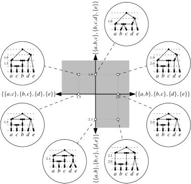
Figure 10. The gray squares represent three orthants of maximum dimension in the orthant space $\mathfrak{S}(X)$ for $X=\{a,b,c,d,e\}$. These orthants are actually 4-dimensional. They are projected into the plane by showing only two of the four coordinate axes that determine each of them (each coordinate axis is labeled by a cluster system in $\mathfrak{T}(X)$; the two axes corresponding to the cluster systems $\{\{a\},\{b\},\{c\},\{d\},\{e\}\}$ and $\{\{a,b,c\},\{b,c,d,e\}\}$ are not shown in the projection). Each point in an orthant corresponds to an ETCN on $X$ with the coordinates of the point describing the difference between consecutive ranks.

One technical aspect, however, also illustrated in Figure 10, is that points that lie on the boundary of an orthant correspond to maps $\omega$ that assign $0$ to certain cluster systems. Intuitively, this means that the cluster system is skipped, leading to a (non-maximal) chain in the poset $(\mathfrak{T}(X),\preceq)$ which then corresponds to a (not necessarily binary) RTCN on $X$ obtained by Theorem 5.2. In view of this, we call a (not necessarily binary) RTCN $\mathcal{N}$ obtained by Theorem 5.2 together with an equidistant weighting of the arcs of $\mathcal{N}$ that is consistent with the ranks of the vertices of $\mathcal{N}$ an equidistant tree-child network (ETCN) on $X$.

A concise, formal description of the continuous space we have just described can be obtained by considering maps $\omega:\mathfrak{T}(X)-\{\{X\}\}\rightarrow\mathbb{R}_{\geq 0}$. For such a map, put ${\rm supp}(\omega)=\{\mathcal{C}\in\mathfrak{T}(X):\omega(\mathcal{C})>0\}.$ Then the orthant-space $\mathfrak{S}(X)$ of all ETCNs on $X$ consists of all maps $\omega:\mathfrak{T}(X)-\{\{X\}\}\rightarrow\mathbb{R}_{\geq 0}$ such that the cluster systems in ${\rm supp}(\omega)$ (together with the cluster systems $\{\{x\}:x\in X\}$ and $\{X\}$), when ordered by $\preceq$, form a chain in the poset $(\mathfrak{T}(X),\preceq)$. More details about the general construction of an orthant-space based on the chains in a poset can be found in (Huber et al.,, 2024, Sec. 4.1). We remark that this construction can also be used to obtain the space of ultrametric trees presented by Gavryushkin and Drummond, (2016) (cf. Huber et al., (2024)).

We now show that the space $\mathfrak{S}(X)$ comes equipped with a distance that has some attractive properties. More specifically, in the theorem below we show that $\mathfrak{S}(X)$ together with the distance $\delta$ that assigns the length $\delta(\omega,\omega^{\prime})$ of a shortest path or geodesic between any two points $\omega,\omega^{\prime}$ in $\mathfrak{S}(X)$ is a CAT(0)-orthant space. Note that this immediately implies that there is a unique geodesic between any two points in $\mathfrak{S}(X)$. As it is quite technical and not important for the proof, we shall not present the definition of CAT(0)-orthant spaces here, but instead refer the reader to e.g. (Miller et al.,, 2015, Section 6) for more details.

Theorem 6.1.

The metric space $(\mathfrak{S}(X),\delta)$ is a CAT(0)-orthant space whose points are in bijective correspondence with ETCNs on $X$.

Proof: It is known (see e.g. Huber et al., (2024, Sec. 4.1) for more details), that constructing a metric space based on a poset in the way that $(\mathfrak{S}(X),\delta)$ was constructed based on the poset $(\mathfrak{T}(X),\preceq)$ always yields a CAT(0)-orthant space.

We now show that the points in $(\mathfrak{S}(X),\delta)$ are in bijective correspondence with ETCNs on $X$. First note that each point $\omega\in\mathfrak{S}(X)$ corresponds to a chain $\mathcal{C}_{1},\dots,\mathcal{C}_{t}$ in $(\mathfrak{T}(X),\preceq)$ that is obtained by ordering the cluster systems in ${\rm supp}(\omega)$ together with the cluster systems $\{\{x\}:x\in X\}$ and $\{X\}$ by $\preceq$. By Theorem 5.2, the chain yields a well-defined (but not necessarily binary) RTCN on $X$. From the values $\omega(\mathcal{C}_{i})$, $1\leq i<t$, we obtain an equidistant weighting of the arcs of this RTCN that is consistent with the ranks of the vertices as described in this section.

Conversely, assume we are given an ETCN on $X$, that is, a (not necessarily binary) RTCN $\mathcal{N}$ on $X$ together with an equidistant weighting of the arcs that is consistent with the ranks of the vertices of $\mathcal{N}$. Let $\mathcal{C}_{1},\dots,\mathcal{C}_{t}$ be the chain in $(\mathfrak{T}(X),\preceq)$ that corresponds to $\mathcal{N}$ by Theorem 5.2. As described in the text, the given equidistant weighting of the arcs of $\mathcal{N}$ yields non-negative values $\omega(\mathcal{C}_{i})$ for all $1\leq i<t$. We formally extend these to a map $\omega:\mathfrak{T}(X)-\{\{X\}\}\rightarrow\mathbb{R}_{\geq 0}$ by putting $\omega(\mathcal{C})=0$ for all $\mathcal{C}\in\mathfrak{T}(X)-\{\mathcal{C}_{1},\dots,\mathcal{C}_{t-1},\{X\}\}$, which then yields the point in $\mathfrak{S}(X)$ corresponding to the given ETCN.  

As an immediate corollary of Theorem 6.1, it follows that the distance between any two ETCNs on $X$, that is, the value $\delta(\omega,\omega^{\prime})$ for the corresponding maps $\omega,\omega^{\prime}\in\mathfrak{S}(X)$, can be computed in polynomial time (Miller et al.,, 2015, Corollary 6.19).

7. Conclusion

In this paper, we have presented various ways to compare binary RTCNs. Interestingly, it is shown by Collienne and Gavryushkin, (2021) that, given two binary ranked trees $\mathcal{T}_{1}$ and $\mathcal{T}_{2}$ on $X$, the rNNI-distance between $\mathcal{T}_{1}$ and $\mathcal{T}_{2}$ can be computed in polynomial time. It would be nice to know if the analogous rNNI^∗-distance between two binary RTCNs defined in Section 4 can also be computed in polynomial time. In this vein, it might also be of interest to consider alternative distances on RTCNs that might arise from generalizing other types of ranked tree modifications (for example, subtree prune and regraft operations (SPRs) considered by Collienne et al., (2024)), or to investigate how the ranked tree distances considered by Kim et al., (2020) might be generalized to RTCNs.

In another direction, it could be worth investigating combinatorial properties of the poset $(\mathfrak{T}(X),\preceq)$. For example, we have shown that this poset is gallery-connected, a property that, for any finite poset, is immediately implied in case the poset is shellable (see e.g. Björner and Wachs, (1983) for a formal definition of shellability). Is $(\mathfrak{T}(X),\preceq)$ shellable? If this were true, then it would immediately imply that the space $(\mathfrak{S}(X),\delta)$ considered in Section 6 has some special topological properties. Note that a similar combinatorial technique was used by Ardila and Klivans, (2006) to understand the topology of spaces of (unranked) equidistant trees.

Finally, Theorem 6.1 implies that methods for performing a variety of statistical computations (e.g. Fréchet mean and variance (Bacák,, 2014; Miller et al.,, 2015), an analogue of partial principal component analysis (Nye et al.,, 2017) and confidence sets (Willis,, 2019)) can be applied (or extended) to the metric space $(\mathfrak{S}(X),\delta)$. These methods allow, for example, the computation of a consensus for a collection of ETCNs. It would be interesting to further explore this possibility, and also to investigate geometric properties of the space $(\mathfrak{S}(X),\delta)$.

References

- Ardila and Klivans, (2006) Ardila, F. and Klivans, C. (2006). The Bergman complex of a matroid and phylogenetic trees. Journal of Combinatorial Theory, Series B, 96(1):38–49.
- Bacák, (2014) Bacák, M. (2014). Computing medians and means in Hadamard spaces. SIAM Journal on Optimization, 24(3):1542–1566.
- Bienvenu et al., (2022) Bienvenu, F., Lambert, A., and Steel, M. (2022). Combinatorial and stochastic properties of ranked tree-child networks. Random Structures & Algorithms, 60(4):653–689.
- Billera et al., (2001) Billera, L., Holmes, S., and Vogtmann, K. (2001). Geometry of the space of phylogenetic trees. Advances in Applied Mathematics, 27(4):733–767.
- Björner and Wachs, (1983) Björner, A. and Wachs, M. (1983). On lexicographically shellable posets. Transactions of the American Mathematical Society, 277(1):323–341.
- Caraceni et al., (2022) Caraceni, A., Fuchs, M., and Yu, G.-R. (2022). Bijections for ranked tree-child networks. Discrete Mathematics, 345(9).
- Cardona et al., (2019) Cardona, G., Pons, J., and Scornavacca, C. (2019). Generation of binary tree-child phylogenetic networks. PLoS Computational Biology, 15(9).
- Cardona et al., (2008) Cardona, G., Rosselló, F., and Valiente, G. (2008). Comparison of tree-child phylogenetic networks. IEEE/ACM Transactions on Computational Biology and Bioinformatics, 6(4):552–569.
- Cardona and Zhang, (2020) Cardona, G. and Zhang, L. (2020). Counting and enumerating tree-child networks and their subclasses. Journal of Computer and System Sciences, 114:84–104.
- Collienne et al., (2021) Collienne, L., Elmes, K., Fischer, M., Bryant, D., and Gavryushkin, A. (2021). The geometry of the space of discrete coalescent trees. arXiv:2101.02751.
- Collienne and Gavryushkin, (2021) Collienne, L. and Gavryushkin, A. (2021). Computing nearest neighbour interchange distances between ranked phylogenetic trees. Journal of Mathematical Biology, 82(1):8.
- Collienne et al., (2024) Collienne, L., Whidden, C., and Gavryushkin, A. (2024). Ranked subtree prune and regraft. Bulletin of Mathematical Biology, 86(3):1–44.
- Fuchs et al., (2024) Fuchs, M., Liu, H., and Yu, T.-C. (2024). Limit theorems for patterns in ranked tree-child networks. Random Structures & Algorithms, 64(1):15–37.
- Fuchs et al., (2021) Fuchs, M., Yu, G.-R., and Zhang, L. (2021). On the asymptotic growth of the number of tree-child networks. European Journal of Combinatorics, 93.
- Gavryushkin and Drummond, (2016) Gavryushkin, A. and Drummond, A. (2016). The space of ultrametric phylogenetic trees. Journal of Theoretical Biology, 403:197–208.
- Gavryushkin et al., (2018) Gavryushkin, A., Whidden, C., and IV, F. M. (2018). The combinatorics of discrete time-trees: theory and open problems. Journal of Mathematical Biology, 76(5):1101–1121.
- Huber et al., (2024) Huber, K., Moulton, V., Owen, M., Spillner, A., and John, K. S. (2024). The space of equidistant phylogenetic cactuses. Annals of Combinatorics, 28(1):1–32.
- Huber et al., (2016) Huber, K. T., Moulton, V., and Wu, T. (2016). Transforming phylogenetic networks: Moving beyond tree space. Journal of Theoretical Biology, 404:30–39.
- Janssen et al., (2018) Janssen, R., Jones, M., Erdős, P., van Iersel, L., and Scornavacca, C. (2018). Exploring the tiers of rooted phylogenetic network space using tail moves. Bulletin of Mathematical Biology, 80(8):2177–2208.
- Jetten and van Iersel, (2016) Jetten, L. and van Iersel, L. (2016). Nonbinary tree-based phylogenetic networks. IEEE/ACM Transactions on Computational Biology and Bioinformatics, 15(1):205–217.
- Kim et al., (2020) Kim, J., Rosenberg, N., and Palacios, J. (2020). Distance metrics for ranked evolutionary trees. Proceedings of the National Academy of Sciences, 117(46):28876–28886.
- Kong et al., (2022) Kong, S., Pons, J., Kubatko, L., and Wicke, K. (2022). Classes of explicit phylogenetic networks and their biological and mathematical significance. Journal of Mathematical Biology, 84(6):47.
- Kuhner and Yamato, (2015) Kuhner, M. and Yamato, J. (2015). Practical performance of tree comparison metrics. Systematic Biology, 64(2):205–214.
- Miller et al., (2015) Miller, E., Owen, M., and Provan, J. (2015). Polyhedral computational geometry for averaging metric phylogenetic trees. Advances in Applied Mathematics, 68:51–91.
- Nakhleh, (2009) Nakhleh, L. (2009). A metric on the space of reduced phylogenetic networks. IEEE/ACM Transactions on Computational Biology and Bioinformatics, 7(2):218–222.
- Nye et al., (2017) Nye, T., Tang, X., Weyenberg, G., and Yoshida, R. (2017). Principal component analysis and the locus of the Fréchet mean in the space of phylogenetic trees. Biometrika, 104(4):901–922.
- Pons et al., (2019) Pons, J., Semple, C., and Steel, M. (2019). Tree-based networks: characterisations, metrics, and support trees. Journal of Mathematical Biology, 78:899–918.
- Robinson, (1971) Robinson, D. (1971). Comparison of labeled trees with valency three. Journal of Combinatorial Theory, Series B, 11(2):105–119.
- Robinson and Foulds, (1981) Robinson, D. and Foulds, L. (1981). Comparison of phylogenetic trees. Mathematical Biosciences, 53(1-2):131–147.
- Smith, (2022) Smith, M. (2022). Robust analysis of phylogenetic tree space. Systematic Biology, 71(5):1255–1270.
- Stadnyk, (2022) Stadnyk, G. (2022). The edge-product space of phylogenetic trees is not shellable. Advances in Applied Mathematics, 135.
- Willis, (2019) Willis, A. (2019). Confidence sets for phylogenetic trees. Journal of the American Statistical Association, 114(525):235–244.