Energetic Analysis of Emerging Quantum Communication Protocols

Abstract

With the rapid development and early industrialization of quantum technologies, it is of great interest to analyze their overall energy consumption before planning for their wide-scale deployments. The evaluation of the total energy requirements of quantum networks is a challenging task: different networks require very disparate techniques to create, distribute, manipulate, detect, and process quantum signals. This paper aims to lay the foundations of a framework to model the energy requirements of different quantum technologies and protocols applied to near-term quantum networks. Different figures of merit are discussed and a benchmark on the energy consumption of bipartite and multipartite network protocols is presented. An open-source software to estimate the energy consumption of photonic setups is also provided.

1 Introduction

With the end goal of constructing a global quantum internet [1], quantum networks are rapidly developing and are already entering a deployment phase. Several national and international initiatives [2, 3] are already in place to establish an architecture allowing for distant nodes to perform quantum cryptographic tasks, such as secret key exchange. In a world with finite resources where energy demands outgrow energy generation, it is therefore crucial to estimate how much energy these networks will consume prior to their deployment [4]. Such a study can reveal limiting factors for future implementations of networks, or even show the energetic advantages of certain quantum technologies over classical ones. Works that estimate the energetic cost of quantum devices are few, but there are indications [5, 6] that quantum computing may show an energetic advantage before a computational one.

Comparing classical and quantum communication protocols in terms of energy is a difficult task, mainly because there are no classical equivalents to most quantum networking protocols with the same level of security. For example, a quantum key distribution protocol achieving information-theoretic security cannot adequately be compared to a classical communication protocol providing only computational security. It is possible, however, to compare different quantum protocols achieving the same functionality. The focus of this study will be put on this task in addition to benchmarking the effective energy consumption of near-term quantum communication infrastructures.

This work presents the foundations of a framework to estimate the energy cost of quantum network protocols. A first estimation is given of the energy requirements of basic network functionalities, namely Quantum Key Distribution (QKD) and Conference Key Agreement (CKA), whose goals are to generate a secret private key among end users of a quantum network. The methods and hardware they use are generic to most protocols based on photonic implementations. In particular, the creation and sharing of entangled states among distant parties, believed to be the main goal of most quantum network architectures [7], are the building blocks of many other network protocols [8, 9, 10, 11, 12, 13].

To obtain concrete figures of merit, we take a hardware-dependent approach to compare different implementations of some common protocols. Namely, different QKD implementations are compared, and the implementation of networks of $N$ nodes are analyzed, since their scaling in resources with the number of nodes is non-trivial. Using the energetic cost as a benchmark, instead of the rate or the fidelity, gives a unique perspective. For example, our simulations suggest that there exists regimes of parameters for QKD protocols where using less efficient but more energy effective detectors results in huge energy savings at the cost of increased execution time. Another example of results from this work are the discovery of distance regimes for which the usage of different wavelengths results in energy savings, and the identification of optimal protocols to achieve multipartite tasks as a function of the number of parties.

This work is organised as follows: first, the model for estimating the energy consumption of photonic setups is introduced in Section 2. The estimation of the energy costs of bipartite QKD protocols is presented in Section 3 and that of multipartite network protocols, in Section 4. To improve readability, the table of hardware components that was used as reference is deferred to Appendix A and the description of the modelling of their energy consumption, to Appendix B. Appendix C contains the description of the QKD protocols that were simulated, and additional results on time-bin based setups are presented in Appendix D, Appendix E displays experimentally measured energy values, and Appendix F touches on the distribution of the power consumption between the users.

2 Energy model

The energy cost of any quantum network protocol can be divided into multiple contributions, which can be studied independently to estimate the total energy cost of the protocol. The first contribution is the source, a broad term encompassing all the required components to generate the state of light onto which the information is encoded. The second contribution to the energy cost regroups all manipulations required in the protocol which include, for example, changes in polarization applied through motorized waveplates, phase shifters, and so on. The third is the detection where the optical signal is measured. Finally, the last contribution comes from classical communications and computations that are required by the protocol.

We define the total energy cost for a protocol $\pi$ as the function $E_{\pi}(t)$ which depends on time, and is composed of:

$$E_{\pi}(t)= \sum^{n_{S}}_{i}S^{i}_{\pi}(t)+\sum^{n_{M}}_{k}M^{k}_{\pi}(t)+\sum^{n_{D}}_{j}D^{j}_{\pi}(t)+C_{\pi}(t)+E_{\pi}(0).$$ (1)

Here, $S^{i}_{\pi}(t)$, $M^{k}_{\pi}(t)$, and $D^{j}_{\pi}(t)$ represent the energy contribution at time $t$ from the $i$th, $k$th and $j$th components involved in the source, the manipulation and the detection, respectively. These specifications are particularly relevant when considering large networks, since the number of sources $n_{S}$, manipulations $n_{M}$ and detections $n_{D}$ might all scale differently with the number of users. In addition, some components need to be initialized which adds a constant term to the overall energy cost $E_{\pi}(0)$.

On top of optical components, quantum network protocols typically include some classical computing elements that increase the energy cost, and those are denoted as $C_{\pi}(t)$. Two major families of contributions are included in this term. The first one consists of the classical controls of quantum components during the time of the protocol. Here, the costs of different components that are commonly involved in communication protocols are considered, such as time taggers to record timing events. All other classical costs required during a protocol are modelled by considering that an active computer is present at each node involved in the protocol. This covers classical communications and memory costs, or classical sub-protocols such as coin flipping.

The second family of contributions is the energy required for post-processing, which refers to the classical algorithms applied to the outcome of quantum processes. This cost is harder to estimate as it depends on various parameters such as the desired level of security, the classical computing architecture and the choice of post-processing functions that are usually not standardized. In this work, this cost is mostly overlooked. However, this post-processing cost can prove to be non-trivial for some of the protocols studied in this work, especially when considering digital signal processing. This particular cost is discussed in Section 3.3.

Each of these families of elements are expanded in Appendix B. In Table 3, some values are shown of power consumption for different types of devices that are used in the following sections.

3 Energy cost of bipartite protocols: Quantum Key Distribution

In this section, we investigate the energetic cost of different widespread QKD protocols. Specifically, the model presented in this work is tested with the well-known BB84 protocol proposed by Bennett and Brassard [14, 15, 16]. We also explore its entanglement-based version, the E91 protocol [17, 18], along with a measurement-device-independent QKD (MDI-QKD) scheme, which was developed to alleviate security assumptions on the detection devices [19, 20, 21, 22]. Then, we expand the analysis to include Continuous Variable QKD (CV-QKD) protocols [23] based on coherent states. Of particular interest are the Gaussian-modulated protocol GG02 [24] as well as a discrete-modulated approach known as QPSK [25, 26]. This is concluded with a discussion on the cost of the classical post-processing in QKD protocols. All of these protocols are detailed in Appendix C, as well as the model employed to estimate their energy consumption.

3.1 Figure of merit

In this work, two different figures of merit are explored, as they provide different views and benchmarks on quantum communication protocol. Firstly, as per similar works in classical networks [27], the energy efficiency (EE) is defined by:

$$EE[\rm bits/Joule]=\frac{\textrm{Secret key rate [bit/s]}}{\textrm{Power [Joule/s]}},$$ (2)

where the power is simply the sum of the electrical powers of the devices involved in the protocol, given in Table 3. The energy efficiency is a time-agnostic quantity which makes it an interesting figure of merit for running quantum networks. It neglects initialization costs and focuses on the energy required to achieve a certain rate with a given protocol. Note that the rate is mostly fixed by the setup and environmental parameters such as losses and noise and that inputting more energy does not necessarily increase the rate.

The second method used in this work is to fix an objective task, or metric, and study the energy required to achieve this task for different hardware, or resources, while fixing the noise (or fixing the hardware while varying the noise). In the case of QKD protocols, the objective task is fixed as the creation of $N_{\mathrm{target}}$ secret key bits between two parties. The energy required to get $N_{\mathrm{target}}$ bits of secret key with protocol and setup $\pi$ is denoted as $E^{N_{\mathrm{target}}}_{\pi}$, and can be derived from Equation 1:

$$E^{N_{\mathrm{target}}}_{\pi}=E_{\pi}(0)+C_{\pi}^{N_{\rm target}}+\frac{N_{\rm target}}{r_{\mathrm{source}}K_{\pi}}\sum_{i\in\mathcal{H}_{\pi}}P_{i},$$ (3)

where $\mathcal{H}_{\pi}$ are the overall hardware elements of the protocol (including the source, the manipulation and the detection), $P_{i}$ the power of the hardware $i$ (assuming a constant consumption during the execution of the protocol), $r_{\mathrm{source}}$ is the repetition rate, and $K_{\pi}$ the secret key rate of the protocol, in bit per channel use. The execution time of the protocol is $t_{n}=\frac{N_{\rm target}}{r_{\mathrm{source}}K_{\pi}}$. Finally, $C_{\pi}^{N_{\rm target}}$ is the cost of classical computing elements, that depends on the number of target bits.

For discrete-variable protocols, the secret key rate $K_{\pi}$ is derived from the raw key rate $R_{\mathrm{DV}}$ in bit per channel use and is given by the following formula:

$$R_{\mathrm{DV}}=\left(\prod_{i}^{n}\mu_{i}\right)\left(\prod_{j}^{m}p_{j}\right)\left(\prod_{k}^{l}10^{-\eta_{k}L_{k}/10}\right),$$ (4)

where $\mu_{i}$ is the probability of photon emission of source $i$. For each hardware element $j$ involved, the probabilities $p_{j}$ represent their different efficiencies, such as detection efficiencies, coupling efficiencies, and so on. Lastly, $L_{k}$ is the length of the optical fibers $k$ that light should go through with a loss per kilometer of $\eta_{k}$.

Going from raw key to secret key in QKD protocols consists of classical rounds of communication between parties, which use part of the generated bits to assess and amplify the privacy of the rest of the bits. In this study, given the raw key rate, an estimate of the asymptotic secret key rate is given, disregarding, for now, the classical post-processing and finite size effects of these protocols. This gives a theoretical upper bound on the achievable secret key rate. Realistic implementations of QKD protocols always display some noise, quantified by the Qubit Error Rate (QBER) in DV-QKD and by the excess noise in CV-QKD. Estimating those noises is crucial to assess the quantity of secret bits that can be extracted from a string of shared bits. Appendix C explains how to derive the secret key rates $K_{\pi}$ for different protocols.

3.2 Results

To simplify the model for discrete variables protocols, sources are considered as black boxes emitting photonic states at rate $r_{\rm source}$ with the same probability $\mu=0.01$. This encompasses weak coherent sources with low mean photon number per pulse, and SPDC based sources that generate entangled states. All the parameters used in the simulation are summarized in Table 1. The values for the initial energy cost $E_{0}$ and the power consumption of different hardware components can be found in Table 3. The details of how each component is modeled can be found in Appendix B while the protocols are presented in Appendix C.

Symbol	Value	Description
$r_{\rm source}$	80 MHz	Repetition rate of lasers for DV protocols
$\mu$	0.01	Probability of emitting a state from a source
$p_{\rm coupling}$	0.9	Coupling probability into a fiber
$p_{\rm BSM}$	0.5	Success probability of a Bell state measurement
$r_{\rm source}$	100 MHz	Repetition rate for CV protocols
$V_{el}$	0.005 SNU	Electronic noise
$\beta$	95%	Reconciliation efficiency for CV-QKD
$\xi$	$0.01$ SNU	Excess noise
	0.95	Detection efficiency of SNSPDs at 1550 nm
	0.25	Detection efficiency of InGaAs-APDs at 1550nm
	0.75	Detection efficiency of Si-APDs at 780nm
	0.5	Detection efficiency of Si-APDs at 523nm
$p_{\rm det}$	0.7	Detection efficiency of the Balanced Homodyne Detector at 1550nm
	30 dB/km	Fiber loss coefficient at 532 nm
	4 dB/km	Fiber loss coefficient at 780 nm
$\eta_{\rm fiber}$	0.18 dB/km	Fiber loss coefficient at 1550 nm

Table 1: Baseline simulation parameters. The first section of rows corresponds to DV parameters, while the second refers to CV parameters. The last two are detector efficiencies and fiber loss coefficients for different wavelengths.

For readability, additional results are shown only in the appendices, in particular a study with time-bin encoding in Appendix D, a study comparing theoretical values to real world measurements of the energy consumption of different pieces of hardware in Appendix E, and a study of the distribution of the power consumption between parties in Appendix F. Interested readers are also invited to use the open-source library [28], which was developed specifically for this work, with their own components and protocols to estimate the energy cost of the experiments.

3.2.1 Comparison of DV-QKD protocols

Three different DV-QKD protocols are compared: BB84, E91 and MDI-QKD. Their description can be found in Appendix C.

In Figure 1, the energy efficiency of these protocols is compared. To obtain a fair comparison, the same set of Superconducting Nanowire Single-Photon Detector (SNSPDs) is considered for all three protocols. It is to be noted that the lasers used in BB84 and MDI-QKD are the same, but the laser used in the SPDC source for entanglement-based QKD works at a different wavelength. The energy cost $E^{\textrm{1 Petabit}}$ of producing $10^{15}$ secret key bits with the same protocols is shown in the inset.

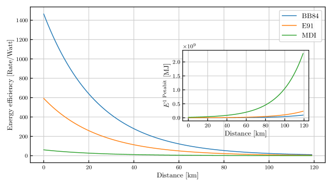
Figure 1: Main plot: Comparison of the energy efficiency of three DV-QKD protocols. Inset: Energy required to produce 1 Petabit of secret key with these protocols.

From this plot, it is clear that, for all distance regimes and using comparable hardware, BB84 is the most energy efficient QKD protocol, followed by E91 and then by MDI-QKD. With the dominating influence of detection apparatus in terms of energy consumption (see Table 3 and Appendix F), one could have expected E91 to be the worst performer due to using more detection stations. However, key rates orders of magnitude lower in MDI-QKD make it the most energy consuming, as shown in Table 2. Importantly, some qualitative advantages present in some protocols, like device independence, are not quantified in any way in this research.

Protocol	Power (Joule/s)	Secret key rate (kbit/s)
BB84	3916	1092.734
E91	8277	934.287
MDIQKD	4070	46.714

Table 2: Energy consumption and secret key rate at a distance of 40 km of the three DV-QKD protocols.

It should be noted that the energy efficiency, as a figure of merit, does not encompass the initialization costs of the devices. It focuses on the energy consumption of a running network, where a specific amount of power is necessary to achieve a given rate. In the inset of Figure 1, it can be seen that the result is indeed the same as what can be observed when using the protocols to generate large numbers of secret key bits. For a large $N_{\mathrm{target}}$ (here 1 Petabit), the initialization costs are absorbed in the running cost of the setup.

This result does not necessarily hold when considering a network running only for a specific task, more likely to be observed in the near-future. In Figure 2, the energy consumption $E^{\rm 1Gbit}$ of the three different DV-QKD protocols is compared for the specific task of producing 1 Gbit $=10^{9}$ bits of secret key.

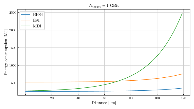
Figure 2: Energy required to distill 1 Gbit of secret key using different choices of DV-QKD protocol.

Here, BB84 remains the protocol with the smallest energy consumption for all distances due to its high rate and the fact that it involves fewer components. The entanglement-based protocol includes two detectors and turns out to be the most energy consuming protocol for distances under 70 km, mainly because of the initialization cost of the detectors. After this distance, the lower success rate of MDI-QKD protocols makes it more energy consuming than the other two options. However, the success rate of MDI-QKD protocols is known to be improvable through the addition of quantum memories that keep unmatched qubits until another one arrives from the lossy channel. This improvement, which also comes with an increased energy consumption attributed to the memory, is not taken into account in this study.

While the energy efficiency might be more useful in the future, when networks are constantly running, the energy required to perform a specific task gives a more precise idea of the current cost of quantum network protocols, in which initialization costs cannot be neglected.

3.2.2 Hardware study

The influence of different hardware choices on the energy cost of an implementation of the BB84 protocol can be observed in this section. The common task $E^{\rm 1Gbit}_{\rm BB84}$ was chosen to display the effects of different hardware. Equipment not considered in this study can be added to the open-source library [28].

The most common implementation of BB84 involves a weak coherent state source with the probability of having one photon in a pulse given by $\mu=0.01$, emitting at 1550 nm. The photons are then coupled into a fiber and detected with SNSPDs of efficiency $p_{det}=0.95$. In Figure 3, $E^{\rm 1Gbit}_{\rm BB84}$ is shown for different QBERs. In general, the QBER is separated into two components, one for each measurement basis of the BB84 protocol. It depends on various hardware parameters and is not a straightforward function of the distance between the parties. It can be optimized for a given setup and a QBER of 2%, which was recently reported for different distances in metropolitan implementations of the protocol [2].

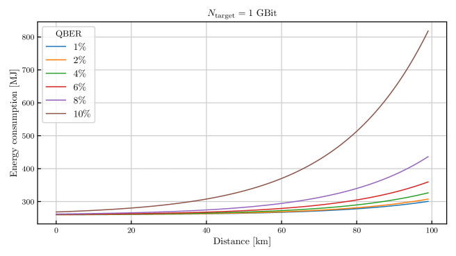
Figure 3: Energy required to distill 1 Gbit of secret key using a polarization WCP-based BB84 setup, as a function of the distance, for different QBER.

To achieve up to 95% detection efficiency at $\lambda=1550$ nm, SNSPDs are required. They rely on cryogenic systems that are the main sources of energy consumption in a photonic setup (see Appendix F). In addition to long cooling times, which can take up to 24 hours, these cryogenic systems require large amounts of energy while they run, as they need to maintain the very low temperatures at which the detectors function. In Figure 4(a), we compare the energy consumption of an SNSPD-based setup to one using Avalanche Photodiode Detectors (APDs). APDs require much less starting time and consume less energy than SNSPDs, as they do not require cryogenics, at the cost of a detection efficiency of 25% at telecom wavelength. As shown in Figure 4(a), using APDs consumes less energy for distances up to 100 km. While the time it takes to obtain 1 Gbit of secret key is higher, the energy consumption is lower. This example illustrates a trade-off between resource cost and efficiency that can also be observed in other energy studies [4, 5]. There is an interest in choosing the energy cost as a benchmark over time: for example at 25 km, considering the same QBER, it takes on the order of 10 min to generate 1 Gbit of secret key with SNSPDs while it is around 30 min using APDs, but the energy required for the SNSPD-based setup is 60 times higher. Since the APDs can also induce more noise such as higher dark count rates, their energy consumption is also shown with a higher QBER. With a QBER of 5%, there is still a large regime where the APDs consumes less energy than the SNSPDs.

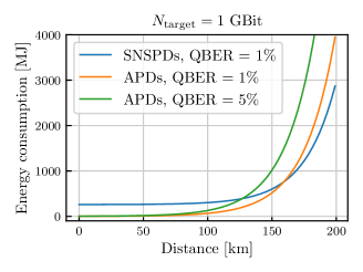
(a) Comparison of the energy required to distill 1Gbit of secret key using highly efficient but energetically costly SNSPDs and less efficient, potentially noisier, but less energetically costly APDs.

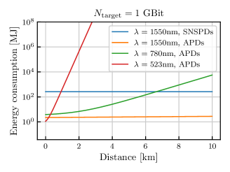
(b) Energy required to distill 1Gbit of secret key using different choices of wavelengths $\lambda$, in logarithmic scale.

Figure 4: Influence of hardware choices on the energetic consumption of BB84.

To obtain higher detection efficiency without using cryogenic-based detectors, working at other wavelengths can be interesting. Besides the telecom range around $\lambda=1550$ nm, typical wavelength choices are near infrared ($\lambda=780$-800 nm) and visible ($\lambda=523$-532 nm). Devices for those wavelengths are included in Table 3. $E^{\rm 1Gbit}_{BB84}$ is shown in Figure 4(b) using different choices of wavelength. The critical difference between the wavelengths is the transmissivity of the fiber, as can be seen in Table 1. After 7 km of distance, working at telecom wavelengths becomes more efficient, even considering cryogenic-based detectors. It is however interesting to note that for short ($<5$ km) or very short ($<300$ m) distances, using infrared or visible wavelength can result in a lower energy consumption than the standard SNSPD-based setup at telecom wavelength. The APD-based setup at $\lambda=1550$ nm is still consuming less energy in most distance regimes, but at the cost of a lower detection efficiency. In a full-scale quantum network, it might thus be useful to consider using different wavelengths depending on the distance between all the parties involved, to optimize both the overall energy consumption of the network and the detection efficiency.

3.2.3 Continuous Variable QKD

The study performed in this section pertains to CV-QKD protocols, but could be adapted to coherent classical communication protocols, as they use similar hardware. Indeed, the usual setup is based on standard telecom technologies, i.e., at a wavelength of $1550$ nm, and Balanced Homodyne Detectors (BHDs) with typical efficiencies above $p_{det}=0.7$, and electronic noise around $V_{el}=0.005$ SNU, in agreement with recent advances in the field [29, 30]. Other parameters used for this section can be found in Table 1. In particular, we choose a higher source rate $r_{\rm source}=100$ MHz than in the case of DV-protocol, which is representative of the latest CV-QKD experiments [23].

Figure 5(a) shows $E^{\rm 1Gbit}_{\text{Gaussian CV-QKD}}$ for homodyne- and heterodyne-based detections, as well as single- and double-polarizations. It can be observed that, for short and medium distances, the overall energy consumption remains constant and is given by the startup energy of the setup. For distances beyond 100 km, however, there is a clear advantage in using a double-polarization scheme since it reduces the overall execution time of the protocol without noticeably increasing the power consumption. Furthermore, the homodyne approach provides a slight improvement in terms of energy for very long distances. The similarity between the homodyne and heterodyne cases is explained by the fact that, while a heterodyne detection measures both quadratures for every round which increases the rate, it then requires two homodyne detection setups which increases the energy cost. Said cost could be reduced by using the RF heterodyne detection scheme, where the two quadratures can be measured with a single balanced detector [31]. These two effects were observed to mostly cancel out, with a slight outperformance of the heterodyne setup. This could nonetheless represent an advantage in terms of scalability for networks of many users.

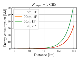
(a) Energy required to distill 1 Gbit of secret key using a Gaussian modulation. The variance of the states was optimized with respect to the distance.

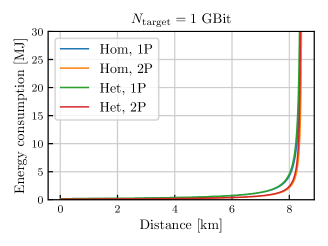
(b) Energy required to distill 1 Gbit of secret key for the QPSK scheme. The amplitude of the states was optimized with respect to the distance.

Figure 5: Study of the energetic consumption of CV-QKD protocols.

The energy consumption of the QPSK protocol is shown in Figure 5(b). The experimental setup is identical to the Gaussian modulation scheme with the corresponding detection apparatus. As in the previous case, the double-polarization provides a clear reduction in the energy consumption, and both homodyne and heterodyne detections provide an overall similar performance. At low distances, the energy consumption does not differ compared to using Gaussian-modulated states. This is explained by the fact that the same hardware setup is considered for both Gaussian and QPSK modulation, and the latter has a considerably lower key rate at high distance. This advantage of the Gaussian distribution is however affected by the inclusion of the cost of classical post-processing, as the digital signal processing and error reconciliation steps may prove to be less energy costly for discrete modulations. Other discrete modulations may also prove more efficient such as Quadrature-Amplitude Modulation, which may make use of a Probabilistic Constellation Shaping [32].

3.3 Classical costs and comparison between CV-QKD and DV-QKD

Results from Figure 4(a) and Figure 5(a) hint at CV-QKD being less energy consuming than any DV-QKD protocols. However, in order to get a meaningful comparison between DV- and CV-QKD protocols, one has also to consider the energetic costs of classical post-processing, which are referred to as classical costs in the rest of this section. In addition to being challenging to estimate, they also largely differ from one family of protocols to the other.

We consider the following contributions to the classical costs: signal processing, parameter estimation, secret key rate computations, information reconciliation and privacy amplification. Except for signal processing and information reconciliation, we assume that the same techniques can be used for DV and CV protocols, and hence that the energetic costs are the same. These contributions can thus be ignored in the comparison between the protocols.

In practice, the biggest difference between CV- and DV-QKD is the digital signal processing (DSP). Indeed, in the DV case, where the photons are detected using single photon detectors, the signal processing is mostly done by the time tagger, that has a known energy consumption and is taken into account in the DV setups. On the other side, recent CV-QKD setups ([23, 31, 33]) are using advanced digital signal processing techniques, which are more costly in energy, and cannot be fully realized in real-time at the time of writing of this paper. Note that information reconciliation cost may also differ significantly between CV- and DV-QKD, as error correction for complex variables is more involved than the one for binary variables. However, estimating the difference between the two costs is not trivial, and is not considered in this analysis.

In CV-QKD, the signal is acquired by the Analog-to-Digital Converter (ADC), and then a series of filters and classical algorithms are applied to recover the symbols. We make the assumption that the cost to recover one symbol from the original signal is a constant and denote it as $\tau_{DSP}$. The energy contribution from signal processing is then given by $\tau_{DSP}$ multiplied by the number of symbols exchanged over the quantum channels:

$$E_{DSP}=\tau_{DSP}\frac{N_{\mathrm{target}}}{K_{\mathrm{CV-QKD}}},$$ (5)

where $N_{\mathrm{target}}$ is the target number of bits in the final secret key and $K_{\mathrm{CV-QKD}}$ is the secret key rate of the CV-QKD protocol (in bit/symbol).

To get an estimate of $\tau_{DSP}$, the open source QOSST software [31] is used as reference, where the DSP runs on a computer during 3 min for 1 million symbols. Assuming a power of 100 W for the computer, this gives an already-achieved value for $\tau_{DSP}=0.018$ J/symbol. Since the software is written in Python, its running time could be optimized greatly, and a value of 1 min for 1 million symbols could be reached in the near future, which would give a slightly more optimistic value $\tau_{DSP}=0.006$ J/symbol.

The costs of the BB84 protocol with APDs and with SNSPDs, as well as the costs of Gaussian-modulated CV-QKD without DSP and for $\tau_{DSP}=0.006$ or $0.018$ J/symbol are shown in Figure 6 . The results reveal that, when neglecting the DSP cost, CV-QKD always outperform BB84. However, with the DSP cost, there is only a small regime of distances (below 5 km) where CV-QKD is more efficient than BB84 with APDs. For high distances ($>75$ km) even BB84 with SNSPDs consumes less than CV-QKD.

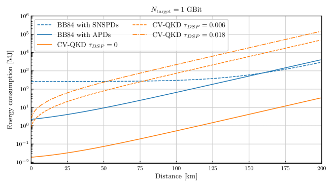
Figure 6: Comparison of the energy consumption of a DV-QKD BB84 implementation with APDs detectors, SNSPDs detectors and energy consumption of CV-QKD with Gaussian modulation, heterodyne measurement and double polarization, including the classical costs from Digital Signal Processing (DSP).

Additionally, note that the DSP cost is independent of the repetition rate $r_{\rm source}$, as seen in Equation 5. While increasing the repetition rate of the protocol results in a lower execution time, it does not significantly decrease the overall consumption as the DSP contribution is several orders of magnitude higher than the time contribution. With the same parameters used for the previous simulation, the classical contribution becomes of the same order of magnitude as the time-dependent hardware contribution when $\tau_{DSP}\sim 10^{-6}$ J/symbol. This shows that classical contributions should not be neglected as part of the energetic analysis, and stresses the need for efficient classical post-processing for quantum communication protocols.

4 Energy cost of multipartite protocols

Protocols involving three or more nodes in a quantum network are of particular interest for future deployments of the quantum internet. Not all quantum technologies scale linearly, and therefore it is worth finding, energy-wise, optimal configurations for multipartite networks. Firstly, different methods of generation of all-to-all entanglement are described and compared. Secondly, Conference Key Agreement (CKA) is used as a figure of merit for multipartite networks by comparing the performances of a few protocols constructed from DV and CV sources.

4.1 All-to-all entanglement

All-to-all entanglement generation is the task that consists in creating quantum correlations between the $n$ parties of a network. It can be envisioned as a building block protocol for most multipartite quantum networks: the network continuously generates entanglement between all the parties who can then manipulate and measure their qubits appropriately to reach a desired quantum state for communication or computation.

The most straightforward method to generate multipartite quantum correlations is for one central party to create a state exhibiting genuine multipartite entanglement [34] such as the GHZ state [35]:

$$\left|\mathrm{GHZ}\right\rangle_{n}=\frac{1}{\sqrt{2}}(\left|0\right\rangle^{\otimes n}+\left|1\right\rangle^{\otimes n}).$$ (6)

GHZ states are prime candidates for network applications since they allow the sharing of entanglement between all nodes at once, as seen in many network protocols [10, 12, 36]. A common photonic GHZ state creation setup involves SPDC sources creating Bell pairs that go through a fusion operation which is inherently probabilistic (see Appendix B.3). As a consequence, the probability of successfully creating a GHZ state of $n$ qubits decreases exponentially with $n$.

In Figure 16, an example is shown for $n=4$ for both time and polarization encodings. For polarization encoding, the energy cost is given by:

$$E_{\rm GHZ}(n,t)=\left\lceil{\frac{n}{2}}\right\rceil\;S_{\textrm{SPDC}}(t)+\left\lfloor{\frac{n-1}{2}}\right\rfloor\;M_{\rm fusion,polarization}(t)+n\;D_{\rm SNSPD}(t)+C_{\rm GHZ}(t),$$ (7)

where $\left\lceil{x}\right\rceil$ (resp. $\left\lfloor{x}\right\rfloor$) is the integer superior (resp. inferior) or equal to $x$. As before, we model the classical cost $C_{\rm GHZ}(t)$ with a computer in each node involved in the protocol, to perform time-tagging or to record the output.

All-to-all entanglement can also be realized through bipartite Bell pairs shared between all pairs of nodes in the network. This architecture requires an SPDC source producing photon pairs in a Bell state between each pair of parties, with each party equipped with single-photon detectors. The energy associated with such an architecture is given by:

$$E_{\rm Alltoall}(n,t)=\frac{n(n-1)}{2}\;S_{\textrm{SPDC}}(t)+n(n-1)\;M_{\rm polar}(t)+n\;D_{\rm SNSPD}(t)+C_{\rm Alltoall}(t).$$ (8)

While this second method amounts to more hardware involved, the low probability of success of high order GHZ state creation requires more repetitions and thus longer running times of the hardware. As shown in Figure 7, the best method to share entanglement between all nodes of a network varies with the number of parties. After $n=6$ parties, the probability of successfully creating a GHZ state becomes so low that it is better, energy wise, to use a pair-wise entangled architecture for this task.

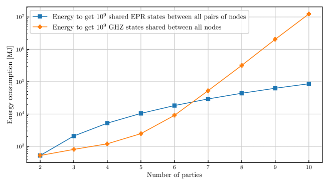
Figure 7: Comparison of the energy required to distribute $10^{9}$ entangled states between $n$ nodes of a network as a function of $n$, in log scale. All the parties are separated by an equal distance of $d=10$ km.

4.2 Conference key agreement

Conference key agreement (CKA) [37] is the multipartite extension of QKD, allowing $n$ parties to create and share a common secret key. Similarly to QKD, there are several protocols that achieve CKA, each with different pros and cons in terms of rate, security bound, and, as per the purpose of this work, energy consumption.

This section considers a quantum network of $n$ parties where one central party (Alice) shares states with the others that are denoted as $\{B_{i}\}_{i=1}^{n-1}$ (Bobs). For simplicity, we consider that all $B_{i}$ are at equal distances from Alice.

4.2.1 DV-CKA

GHZ state implementation

The most straightforward method to create a secret key between $n$ users of a quantum network is to distribute the qubits of a GHZ state to each party of a network. By measuring their qubits in the appropriate bases, the parties automatically extract a common bit, whose privacy follows from the monogamy of entanglement. A full security proof and description of a GHZ-based CKA protocol can be found in [38], while an experimental realization can be found in [39]. The rate of this protocol, which we denote GHZ-CKA in the following section, is given by the rate of creating, sharing, and measuring GHZ states that were distributed to the $n$ parties. Assuming that all $n$ parties are at an equal distance $d$ from the source of GHZ states, Equation 4 becomes:

$$R_{\rm GHZ-CKA}(n)=r_{\rm source}\;\mu^{\left\lceil{\frac{n}{2}}\right\rceil}\;p_{\rm coupling}^{n}\;p_{\rm det}^{n}\;10^{n\;\frac{\eta_{\rm fiber}d}{10}},$$ (9)

where $d$ is the distance between the source of GHZ states and the parties. As per previous sections, this rate allows the estimation of the time necessary to create a certain objective number of secret key bits between the $n$ parties. Equation 7 can then be used to get the energy cost.

Parallel bipartite implementations

Alternatively, a conference key can be built from $n-1$ bipartite secret keys. Indeed, imagine that Alice shares keys $\{k_{i}\}_{i=1}^{n-1}$ with each Bob $B_{i}$. She can choose one of these keys, say $k_{1}$, to be the conference key and send it securely to each $B_{i}$. This can be done, for example, using the one-time pad protocol. More explicitly, for each $i\neq 1$, $k_{1}$ is sent to $B_{i}$ encoded with its corresponding key $k_{1}\oplus k_{i}$. $B_{i}$ can recover $k_{1}$ by using their key $k_{i}$. Two other approaches to CKA are hence considered. In the first one, that we identify as BB84-CKA, Alice performs the BB84 protocol presented in Section C.1.1 with each Bob. In the second approach, that we name Bell-CKA, Alice performs the entanglement-based QKD protocol presented in Section C.1.2 with each other party of the network. The comparison between these protocols is illustrated in Figure 8. Other approaches could be envisioned, where a bipartite key is done in parallel between pairs of parties, but those do not compare as directly with the GHZ approach.

In the simulations, we assume that all bipartite QKD links work simultaneously, in parallel. Achieving the objective number of shared bits between all nodes therefore requires a time equal to achieving that objective between two nodes only. The total number of sources required in this scenario scales with the number of parties $n$. In the Bell-CKA scenario, the number of detectors scales as $2n$. The total energy cost is then proportional to the total number of links.

4.2.2 CV-CKA

Multipartite Gaussian state implementation

For continuous variables, a CKA protocol based on the distribution of Gaussian-modulated coherent states is considered, following [40]. In said protocol, each of the $n$ Bobs individually prepares a copy of an initial state for every round, and all states are sent to a central node where a series of generalized Bell measurements are performed. Namely, a cascade of beam splitters and homodyne detections are applied on the states, such that $n-1$ measurements are performed on the first quadrature and only one measurement is performed on the second. The correlations generated at the beam splitters ensure that all the parties can generate a shared key. In this scenario, the energy model is provided by the following setup: each of the Bobs requires a computer, a laser, an IQ modulator, an MBC, and a DAC. The detection is composed of $n$ homodyne detectors that always measure the same quadrature such that no active phase modulation is necessary, as well as $n-1$ beam splitters which are passive components. The data is then acquired using an ADC where we denote the number of channels as $n_{\rm chan}$. For the subsequent simulations, we consider $n_{\rm chan}=4$ and the value provided for the ADC in Table 3. Furthermore, we assume that the central detector is linked to one computer that post-processes the measurement outputs. All in all, the energy is given by:

$$E_{\mathrm{CV-CKA}}(n,t)=ntP_{\mathrm{B,source}}+tP_{\mathrm{det}}(n),$$ (10)

where:

$$P_{\mathrm{B,source}} =P_{\mathrm{laser}}+P_{\mathrm{MBC}}+P_{\mathrm{DAC}}+P_{\mathrm{PC}},$$ (11)

$$P_{\mathrm{det}}(n) =nP_{\mathrm{BHD}}+\left\lceil\frac{n}{n_{\rm chan}}\right\rceil P_{\mathrm{ADC}}+P_{\mathrm{PC}}+nP_{\rm laser}.$$ (12)

A brief description of the method to compute the secret key rate of the protocol [40] is given in Appendix C.2.3. As a concluding remark, each of the Bobs needs to perform post-processing of the measured outcomes, which means that the classical cost increases with the number of users (see Section 3.3).

Parallel bipartite implementation

It is possible, as with DV-QKD approaches, to distill a conference key out of $n$ bipartite keys created with CV-QKD protocols. Consider a centralized CV-QKD network, i.e., $n-1$ users (Bobs) connected to a central node (Alice). Each Bob individually distills a key with Alice using the CV-QKD protocol presented in Appendix C.2. More precisely, a Gaussian-modulated CV-QKD protocol is considered, with homodyne measurements and double-polarization. All the parties can then create a common key by mixing the individual, bipartite keys, as explained before. We identify this CKA protocol as the nCV-QKD protocol.

4.2.3 Simulation results for CKA

For the GHZ-CKA protocol, the central node Alice creates $n$-qubit GHZ-states, keeps one qubit to herself and shares each other one to each $B_{i}$. For the Bell-CKA protocol, in the same fashion, Alice creates sequentially $n-1$ Bell pairs, keeps one qubit of each pair to herself and sends the other one to each $B_{i}$. Finally, for the BB84-CKA protocol, Alice sends single photons in the form of weak coherent pulses to each of the $B_{i}$. Note that the Bell-CKA and the BB84-CKA protocols involve an additional round of classical communication between Alice and each of the Bobs after the quantum key distribution rounds.

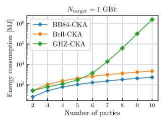
(a) Energy consumption of the three different CKA setups as a function of the number of parties for a fixed distance between the parties and the central node of 5 km, in log-scale.

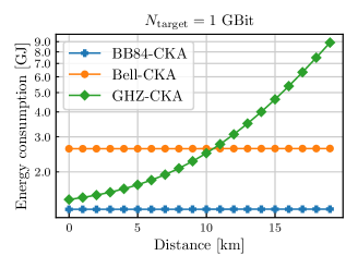
(b) Energy consumption of the three different CKA setups as a function of the distance between the parties and the central node, for a fixed number of parties $n=5$, in log-scale.

Figure 8: Energetic analysis of DV-CKA protocols.

In Figures 8(a) and 8(b), the energy cost $E^{\textrm{ \rm 1Gbit}}_{\textrm{CKA}}$ required to create 1 Gbit of key is illustrated, using the three aforementioned DV-CKA protocols as a function of the number of parties and as a function of the distance with the middle party Alice. The BB84-CKA protocol is always more energy efficient than the other two options. This is due to the high rate and high success probability of the BB84 protocol. As for the All-to-all task, there is a regime for both the number of parties and for the distance for which the GHZ-CKA protocol is more energy efficient than the Bell-CKA protocol. For longer distances and for higher numbers of parties, the probability of a successful generation and detection of a GHZ state decreases to the point where it becomes more efficient to use bipartite communications between Alice and each Bob to accomplish this task.

These studies show that the energy required to create and share GHZ states grows exponentially with the number of parties. Small scale networks can benefit from GHZ-based protocols. Nonetheless, for large number of users, more efficient schemes for GHZ-state creation need to be developed to reasonably envision quantum networks based on multipartite entanglement.

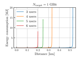
(a) Energy consumption required to distill 1Gbit of key with the CV-CKA protocol as a function of the distance with the central node, for different numbers of users.

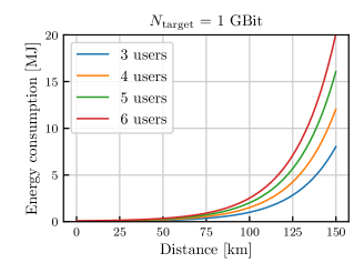
(b) Energy consumption required to distill 1Gbit of key with the nCV-QKD protocol (using homodyne measurements and double-polarization) as a function of the distance with the central node, for different numbers of users.

Figure 9: Energetic analysis of CV-CKA protocols.

The energy consumption required to create 1 Gbit of secret key using the CV-CKA protocol of [40] as a function of distance is shown in Figure 9(a) for different numbers of parties. Regarding the comparison between continuous and discrete variables, the energy consumption of the CV-CKA protocol is three orders of magnitude lower than its DV-counterpart, but with major limitations on the achievable distance since this energetic advantage is valid only over a few hundred meters [40]. This is therefore a solution to be considered for a few users within building-scale distances, compared to other DV-CKA protocols presented in previous sections.

Figure 9(b) shows the energy consumption required to create 1 Gbit of secret key using the nCV-QKD protocol for diverse numbers of users $n$, all of them separated by the same distance. A similar energy consumption with respect to the CV-CKA approach is observed with a noticeable improvement in terms of achievable distances. Both techniques employ vastly different classical post-processing (in particular, the DSP), such that adding those contributions could modify the results of this simulation.

5 Conclusion

In this article, we laid the foundations of a framework to estimate the energy consumption of quantum communication protocols. Two figures of merit were introduced, namely the energy efficiency and the energy cost required to produce a target number of secret bits. We applied them to different implementations of bipartite and multipartite protocols. The energy efficiency gives an idea of the consumption of a running network while the energy cost of producing a target number of bits gives a benchmark for the current and near-term energy cost of network protocols. By studying the energy cost required to solve identical basic tasks through different protocols and hardware choices, hardware and protocol choices can be optimized.

This first insight into the energetic cost of photonic-based quantum communication protocols, including multipartite scenarios, shows that the critical components in discrete variable protocols are the cryogenic-based hardware, while continuous variable protocols are deeply affected by post-processing. An interesting highlight of this study is that, for a distance of 25 km, a typical BB84 setup could generate 1 Gbit of secret key 60 times more efficiently using a less energy costly but less efficient detector than the usual cryogenic-based detectors, at the cost of 3 times the temporal requirements. These differences are critical at this early stage of quantum network development and can direct future efforts in different directions.

While telecom-compatible technologies are desired for ease of implementation, it was shown that at very small scales, visible and near-infrared wavelengths were consuming less energy than their telecom counterparts. While replacing the whole existing infrastructure is not foreseeable, this result shows that the installation of new small-scale networks could benefit from thoughtful wavelength choices.

Due to their probabilistic nature, multipartite protocols based on GHZ states scale worse over long distances or high number of parties than those based on repeating pair-wise DV-QKD, but show competitive regimes at smaller distance and number of parties. Results might evolve by using new hardware such as dedicated integrated photonic platforms to reduce the energy cost.

Future work will extend this study in several directions. This framework could readily be used to estimate the energy consumption of photonic computation architectures, such as [41]. More consideration must be given to the cost associated to classical post-processing, and in particular to the trade-off between the energy spent in post-processing and the level of security. Since said task is more involved for CV protocols, this might give more insight into which method is more efficient. Furthermore, it is worth considering the authentication cost of the classical channels used by the parties. This is done using pre-shared keys [42] or post-quantum cryptography [43], and is a requirement to avoid man-in-the-middle attacks. The costs of these tasks are difficult to estimate because there is no standard method to perform them yet. Finally, the list of hardware available in the accompanying software can be expanded, including for example new components such as quantum memories or solid-state sources. This will contribute to rigorous benchmarking and optimization of the energy consumption of large scale quantum networks with heterogeneous hardware for each nodes and hybrid fiber/free-space links.

Appendix A Table of components

Laser $\lambda$ (nm) $E_{0}$ (kJ) Meas. (kJ) $P$ (W) Meas. (W) Ref. Verdi C-Series 532 648 360 laser1 Verdi V-Series 532 1620 864 900 480 verdivseries DLC TA pro 795 0 70 laser2 D2547P 1532 0 3 laser3 NKT Koheras Basik X15 1550 0.12 0.126 4 4.2 koherasbasikx15 Mira HP F 780 3240 1800 laser4 SCW 1532-500R 1550 0 2.4 laser5 Detector $\lambda$ (nm) $E_{0}$ (kJ) Meas. (kJ) $P$ (W) Meas. (W) Ref. Si-APD 523 0 45 detector5 Si-APD 780 0 15 detector1 InGaAs-APD 900-1700 48.3 5.04* 161 14 id220 InGaAs-APD 1532 1159 125.7* 644 64 detector2 SNSPD 780 259200 3000 detector3 SNSPD 1532 259200 117639* 3000 2735 detector3 Balanced detector 1550 0 3 6.8 thorlabspdb480ac Component $E_{0}$ (kJ) Meas. (kJ) $P$ (W) Meas. (W) Ref. Computer 9 6 150 100 component1 Time tagger 0 50 22 component3, component9 Motorised Waveplates 0.93 0.249 31 8.3 component2 Interferometry 0 200 laser3,detector6,component8 Modulator (AM) 15 0.78 500 26 component4, MBC-DG-LAB, FI-5682GA Oven (with Controller) 9 0.54 15 0.9 component6 Modulator (IQ) 0.18 0.162 6 5.4 mbciqlab Polarization Controller 0 1.8 0.35 ThorlabsMPC320 Powermeter 0 1 0.8 ThorlabsPM101A Optical switch 0 1.8 0.35 thorlabs-osw12 ADC 0 30 20 teledyneadq32 DAC 0 40 40 teledynesdr14tx

Table 3: Example of components frequently used in laboratories, including information about their power usage, startup time, and other interesting data such as central operating wavelengths, detector efficiencies, and reference documentation. Measured values are also indicated (see below for more details on the experimental procedure).

Theoretical values for $E_{0}$ are obtained by multiplying the initialization time by their power. Measured $E_{0}$ is obtained either by multiplying the initialization time by the measured power, or fully measured by following the power consumption in real time and integrating (marked by an asterisk *).

For the measured values in Table 3 (column 5 and 7), the measurements were done in one of the three following ways, depending on its power connection type:

• If the device could be plugged through a standard power adaptor to a standard electrical outlet, the measurement was done using a power meter socket powermetersocket with a maximal load of 3680 W.

• If the device was plugged to a standard lab power supply, then the measurement was done by applying the required voltage, and recording the consumed current, and multiplying the two values to get the power.

• Finally, if the device was powered through USB, then the consumption was measured by adding a USB adaptor before the power meter socket. This method adds the consumption of the adaptor, but these usually have low power consumption values (USB 3.0 has a maximal output voltage of 5V with a standard requirement of 0.9 A resulting in a typical maximal power of 4.5 W).

When possible the power consumption was measured when the device was being used. The measurements for the lasers were done while emitting their optical beam; for the single photon detectors, while detecting a flow of single photons; for the computers, while they were running the control software of the CV-QKD experiment; for the waveplates, while they were rotating; for the AM modulator, while applying a pulsed signal (for the signal generator) and while locking (for the modulator bias controller); for the oven, while stabilizing a temperature of 25^∘C; for the IQ modulator, while locking the modulator; for the powermeter, while receiving optical power; for for the optical switch, while applying switching commands; for the ADC and DAC, while running the CV-QKD experiment (and hence emitting and receiving signals).

Additionally for some equipment with a long initialization time (such as lasers or single photon detectors), the power consumption was recorded during the initialization.

Appendix B Models for encoding, source, detection and manipulation

This appendix contains details of the models for different source, manipulation and detection elements used in Equation 1.

B.1 Choice of encoding

There are multiple approaches to encode information in a state of light, each with pros and cons, and each involving different hardware to create, control and measure quantum information. For discrete variable (DV) protocols, a simple option is to encode qubits on the polarization of a photon or of a pulse of light. This encoding is of major interest due to easily available passive components, but polarization is susceptible to birefringence which is present in most fiber networks. An alternative is time encoding where two distinct arrival times are defined as the logical zero and one. This type of encoding is also a major contender due to its reliability over long distances, but requires precise control of the phases of the signals due to the necessary use of interferometers.

Continuous variable (CV) protocols rely on quadrature encoding and are readily implementable with commercial telecom components. In quantum optical systems, quadratures are the real and imaginary parts of the electromagnetic field [44], which are usually named in-phase and quadrature components in classical telecommunications [45]. The encoding can be implemented using an IQ modulator and decoded with coherent detection (homodyne or heterodyne). The advantage of this class of protocols is that they can be performed with the same hardware as in the currently deployed telecommunication infrastructure. While they are less resilient to losses compared to their DV counterpart, the higher repetition rate allowed by the detection system usually makes the secure key rate of CV-QKD protocols higher than DV-QKD protocols at metropolitan scale distances  [46].

On a different note, this analysis refers to the most popular schemes of encoding, but other choices not considered in this study (such as frequency, spatial and angular orbital momentum encodings) are possible.

The choice of encoding in communication protocols influences not only the hardware used but also the performances achieved. In this work, we take a minimalist approach, simplifying setups and protocols to the strict minimum functionalities required to make these protocols work, in order to show general behaviors and to showcase the model in different situations.

B.2 Sources

B.2.1 Weak coherent pulse sources

Weak coherent pulse sources are a practical and efficient method to obtain single-photons probabilistically. The idea consists of attenuating a laser pulse until the probability that a light packet contains more than one photon is low enough that it can be neglected or effectively bounded in security proofs. From a hardware point of view, this requires a laser, passive attenuation and, usually, an amplitude modulator.

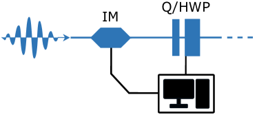
Figure 10: Typical source schematic for weak coherent pulses. The pulses are carved using an intensity modulator, while the polarization is controlled through motorized waveplates. The lasing power can be attenuated at the laser level, or through passive attenuation.

Polarization encoding can be done by adding a series of waveplates. We assume that the waveplates used in the different components and protocols of this study are motorized in order to automatize their calibrations in the context of large networks [47]. This is translated to the following function representing the energy cost:

$$S_{\textrm{weak,polarization}}(t)=t(P_{\rm laser}+P_{\rm modulator}+P_{\rm waveplates}).$$ (13)

For time encoding, interferometry is done through the use of unbalanced Mach-Zehnder interferometers. These devices require an independent weak laser and a classical detector for stabilization purposes, heating elements for temperature control, and a piezo-type element for phase control between the two arms. These are included in a general function called $P_{\rm interferometry}$.

$$S_{\rm weak,time}(t)=t(P_{\rm laser}+P_{\rm modulator}+P_{\rm interferometry}).$$ (14)

B.2.2 Spontaneous parametric down conversion sources

Spontaneous Parametric Down Conversion (SPDC) is a popular, cheap and accessible technology that generates light at the single photon level and that, above all, creates correlated photon pairs that are easy to entangle. While one of the photons of the pair can be ignored when only a single photon is required, many protocols use this second photon as a heralding mechanism [48]. Sources based on SPDC are structurally simple: a pump laser and a non-linear crystal are the minimum requirements to generate single photons. Note that a resistance heater oven maintains the crystal’s temperature.

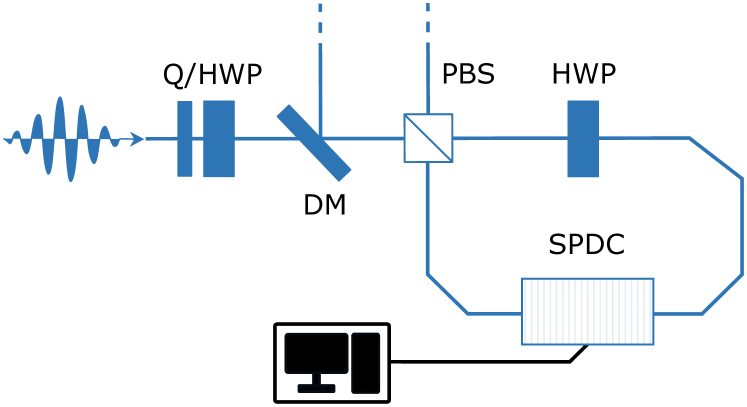
(a) Source for photon pairs entangled in polarization.

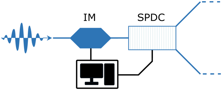
(b) Source for time entangled photon pairs.

Figure 11: Components involved in SPDC sources: a) a laser light is oriented in the $\left|H\right\rangle+\left|V\right\rangle$ polarization state through quarter and half-waveplates (Q/HWP) before entering a Sagnac loop consisting of a Polarized Beam Splitter (PBS), a Half-Waveplate (HWP) and a non-linear crystal in which the pump light undergoes Spontaneous Parametric Down Conversion (SPDC). The created photon pairs exit the loop through the PBS and a Dichroic Mirror (DM). b) Laser light is pulsed into two time bins by an Intensity Modulator (IM) before undergoing SPDC. In both setups, a resistance heater oven maintains the temperature of the crystal.

Polarization encoding is done through waveplates and using a Sagnac loop, as shown in Figure 11(a). The energy cost of a polarization SPDC source is thus given by:

$$S_{\rm SPDC,polarization}(t)=t(P_{\rm laser}+P_{\rm oven}+P_{\rm waveplates}).$$ (15)

For time-bin encoding, interferometry of some type is required to transform a single pulse into two phase-controlled pulses. This can be done directly with an intensity modulator, although methods exist using Mach-Zehnder interferometers and/or phase modulators. The simplest setup, shown in Figure 11(b), gives the following energy cost:

$$S_{\rm SPDC,time}(t) =t(P_{\rm laser}+P_{\rm oven}+P_{\rm modulator}).$$ (16)

B.2.3 Modulated coherent states sources

In CV protocols based on modulated coherent states, one needs to generate coherent states and choose their average quadratures, which can be done by using a laser and an IQ modulator [49], which is itself usually composed of 2 Mach-Zehnder interferometers nested in a third one. Such a source would also include passive attenuators to reach the required low modulation strength, a Modulator Bias Controller (MBC) acting as a feedback loop to lock the modulator around its functioning point, and a photodiode used to monitor the output power and measure the average number of photons per coherent state $\langle n\rangle$ (which for the CV-QKD protocol is related to the modulation strength by $V_{A}=2\langle n\rangle$). A Digital-to-Analog Converter (DAC) connects the controlling computer to the different devices. The typical scheme for the source is presented in Figure 12. The energy cost is given by:

$$S_{\mathrm{CV}}(t)=t(P_{\rm laser}+P_{\rm mbc}+P_{\rm dac}+P_{\rm photodiode}).$$ (18)

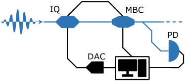
Figure 12: Setup for a coherent source of CV states. Information is encoded by sending an electrical signal from a Digital-to-Analog Converter (DAC) to the IQ modulator, effectively displacing coherent states, while the Modulator Bias Controller (MBC) acts as a feedback loop to lock the modulator on its functioning point. A photodiode (PD) is used to monitor the optical power and measure the modulation strength. A realistic setup would also include optical attenuators and other passive optical elements.

B.3 Manipulation

In this model, the manipulation of quantum states refers to all the electro-optical operations done to a photonic quantum state before detection. These manipulations are essential for almost all schemes since photonic states need to be shaped to perform the protocol or to control the measurement basis. When the information is encoded in the polarization of a photon, manipulation can be done using a series of waveplates before a PBS, with an energy cost given by:

$$M_{\rm polar}(t)=tP_{\rm waveplate}.$$ (19)

Quantum gates for time bins are challenging since they require interferometry again. The energy cost is given by:

$$M_{\rm time}(t)=tP_{\rm interferometry}.$$ (20)

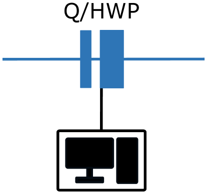
(a) Manipulation of polarization-encoded states

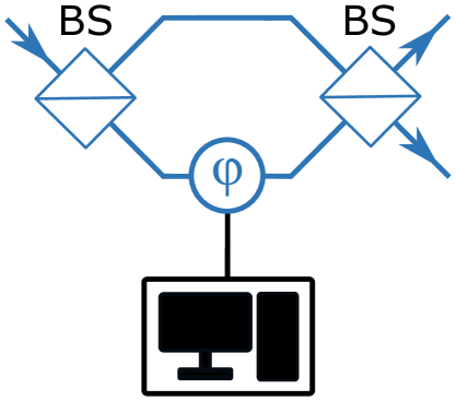
(b) Manipulation of time-encoded state

Figure 13: a) Manipulation station for polarization qubits, which allows for projections over any polarization state. b) Manipulation station for time-bin qubits. It consists of an unbalanced Mach-Zehnder interferometer with phase control in one arm.

Some network protocols require multipartite entangled states, i.e., states with more than two entangled photons. To create such states, the most common technique is to join two bipartite sources together through an operation called fusion [50, 51, 52, 53]. This process takes one photon from each bipartite source and entangles them to create a four-photon entangled state. Higher orders are then reached by adding fusion stations and sources sequentially. Efficient fusion is challenging, especially with photonic states, since it requires precise timing of events that are inherently probabilistic. Recent progress towards fusion-based quantum computation has, however, shown that fusion of photonic graph-state can be the basis of quantum computers [54].

Figure 14 details a graphical representation of the fusion operation that is considered in this work. Given input channels $A_{2}$ and $B_{1}$ and output channels $x$ and $y$, the logical operation required for fusion is defined as:

$$\left|0\right\rangle_{A_{2}} \rightarrow\left|0\right\rangle_{x},$$ (21)

$$\left|0\right\rangle_{B_{1}} \rightarrow\left|0\right\rangle_{y},$$

$$\left|1\right\rangle_{A_{2}} \rightarrow\left|1\right\rangle_{y},$$

$$\left|1\right\rangle_{B_{1}} \rightarrow\left|1\right\rangle_{x},$$

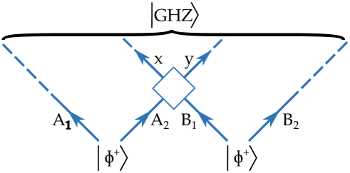
Figure 14: Graphical representation of a generic fusion operation, one of the building blocks of multiparty entangled state creation.

Indeed, acting on one qubit of two independent Bell pairs $\left|\phi^{+}\right\rangle_{A}=\frac{1}{\sqrt{2}}(\left|0\right\rangle_{A_{1}}\left|0\right\rangle_{A_{2}}+\left|1\right\rangle_{A_{1}}\left|1\right\rangle_{A_{2}})$ and $\left|\phi^{+}\right\rangle_{B}$ defined similarly, this logical operation gives:

$$\left|\phi^{+}\right\rangle_{A}\otimes\left|\phi^{+}\right\rangle_{B} =\frac{1}{\sqrt{2}}(\left|0000\right\rangle_{A_{1}A_{2}B_{1}B_{2}}+\left|1100\right\rangle_{A_{1}A_{2}B_{1}B_{2}}+\left|0011\right\rangle_{A_{1}A_{2}B_{1}B_{2}}+\left|1111\right\rangle_{A_{1}A_{2}B_{1}B_{2}})$$

$$\rightarrow\frac{1}{\sqrt{2}}(\left|0000\right\rangle_{A_{1}xyB_{2}}+\left|1100\right\rangle_{A_{1}yyB_{2}}+\left|0011\right\rangle_{A_{1}xxB_{2}}+\left|1111\right\rangle_{A_{1}xyB_{2}}).$$

Assuming post-selection to keep only the states with one photon in each output channel, this eliminates the contributions from the two components in the middle, and leads to:

$$\frac{1}{\sqrt{2}}(\left|0000\right\rangle_{A_{1}xyB_{2}}+\left|1111\right\rangle_{A_{1}xyB_{2}}),$$ (22)

which is a 4-photon GHZ state. Note that this post-selection process is necessary and that it causes the fusion process to be inherently probabilistic. The maximum success probability of photonic fusion achieved via this method is 50%. Higher fusion success probabilities can be reached by adding additional lasers and photonic ancillas [55, 56].

For polarization-encoded qubits, this operation can be done with a PBS. One of the inputs contains polarization compensating waveplates, and therefore the energy cost is given by:

$$M_{\rm fusion,polar}(t)=tP_{\rm waveplate}.$$ (23)

For time-encoded qubits, this operation requires an intensity modulator with two-inputs and two outputs that acts as a very fast switch. This device is connected to an accompanying waveform generator and the power consumption is:

$$M_{\rm fusion,time}(t)=tP_{\rm modulator}.$$ (24)

The schematics of polarization and time fusion are shown in Figure 15, while that of a complete setup to create 4-qubit GHZ states is shown in Figure 16.

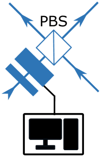
(a) Polarization fusion

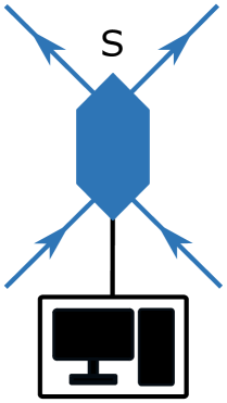
(b) Time fusion

Figure 15: (a) Fusion station for polarization qubits. The transformation required is that of a polarized beam splitter (PBS). (b) Fusion station for time bin entanglement, done by an intensity modulator.

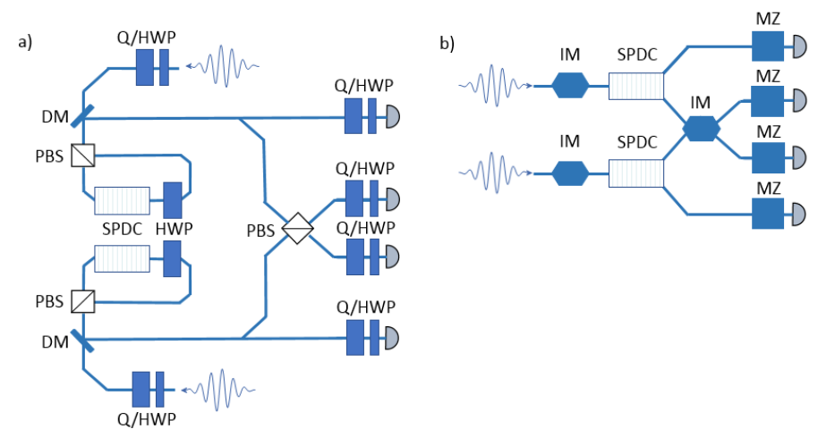
Figure 16: Schematics of setups to create and share 4-qubit GHZ states encoded a) in polarization and b) in time.

B.4 Detection

B.4.1 Single photon detectors

In DV regimes, detection devices are typically threshold detectors, which are greatly influenced by the choice of signal wavelengths. Avalanche Photo-Diode (APD) single-photon detectors work through the ionization of their constituent material at the reception of photons, which creates a current that is in turn amplified. At near-infrared wavelengths, those are readily available and have good efficiencies and low energetic costs that make them an interesting choice (see Table 1 and 3). Superconducting Nanowire Single-Photon Detectors (SNSPDs) have a much higher efficiency at telecom wavelength, as well as small jitters and dead times, allowing for high detection rates and precision. The interaction of the photons with the nanowire creates a temporary resistive region in the superconductive wire, briefly breaking superconductivity and leading to a detectable voltage pulse. SNSPDs are one of the leading choices in current experimental implementations of photonic protocols at telecom wavelength. However, the necessity of cryogenics presents a significant drawback in their energetic cost.

Incorporating essential electronics in the computer present at each node, such as Time-to-Digital Converters (TDC), two energy functions for the detectors can be formulated:

$$D_{\rm APD} =tP_{\rm APD},$$ (25)

$$D_{\rm SNSPD} =tP_{\rm SNSPD}.$$ (26)

B.4.2 Coherent detectors

For CV protocols, detection can be either homodyne or heterodyne. In homodyne detection, a single quadrature of the field is measured. In heterodyne detection, both quadratures of the light field are measured simultaneously at the expense of the addition of extra noise in the signal.

The base device in both scenarios is the same: a Balanced Homodyne Detector (BHD) acts as the core component of the apparatus [49]. It is internally composed of two standard photodiodes and a Trans-Impedance Amplifier (TIA) that transforms the current difference of the two photodiodes into a voltage with a significant gain. The energetic cost of this balanced receiver can be broken down as follows:

$$P_{\rm BHD}=2P_{\rm photodiode}+P_{\rm TIA}$$ (27)

For CV-QKD with homodyne detection, a Motorized Polarization Controller (MPC) and a Switch (S), used respectively to compensate long-distance polarization dispersion and to calibrate the noise levels, receive the light signal and mix it with a Local Oscillator (LO) in a beam splitter. The result is sent to the BHD device. It also requires a phase modulator on the LO path in order to select the measured quadrature (and perform a sifted protocol, as in BB84 for instance). An Analog-to-Digital Converter (ADC) allows the acquisition of data. For heterodyne detection, the general concept is the same, except that the signal light is divided in two. Each of these outputs is separately mixed with the local oscillator, one of the two being dephased by $\pi/2$, before being sent to a BHD each, allowing for simultaneous measurement of both quadratures. The two possible detection schemes are presented in Figures 17(a) and 17(b).

The polarization controller can be avoided by performing a polarization-diverse protocol and performing the polarization compensation digitally. In that case, information can also be encoded on the second polarization. This requires adding a passive polarization beam splitter and a second detection station (with 1 or 2 BHDs depending on homodyne or heterodyne). The cost of the CV detection is given by:

$$\begin{split}D_{\rm CV-QKD,hom,1P}(t)&=t(P_{\rm ADC}+P_{\rm laser}+P_{\rm BHD}+P_{\rm PC}+P_{\rm PM}),\\ D_{\rm CV-QKD,het,1P}(t)&=t(P_{\rm ADC}+P_{\rm laser}+2P_{\rm BHD}+P_{\rm PC}),\\ D_{\rm CV-QKD,hom,2P}(t)&=t(P_{\rm ADC}+P_{\rm laser}+2P_{\rm BHD}+P_{\rm PC}+P_{\rm PM}),\\ D_{\rm CV-QKD,het,2P}(t)&=t(P_{\rm ADC}+P_{\rm laser}+4P_{\rm BHD}+P_{\rm PC}),\\ \end{split}$$ (28)

where $1P$ and $2P$ correspond to single-polarization and double-polarization.

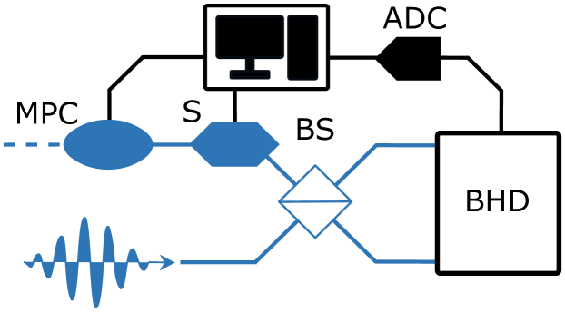
(a) Homodyne detection

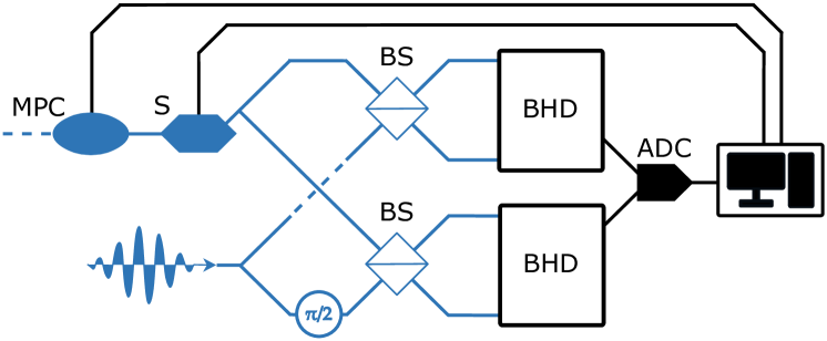
(b) Heterodyne detection

Figure 17: Possible detection schemes for CV-QKD. MPC: Motorised Polarization Controller. S: Optical switch. BS: Beam Splitter. BHD: Balanced Homodyne Detector. ADC: Analog-to-Digital Converter.

B.5 Transfer of photons in fibers

A key component in quantum communications is the quantum channel linking the parties of a network. In this regard, optical fibers are the most common and stable components used to transfer photonic states. Fibers, however, come with the limitation that the probability that a photon is transmitted in the fiber decreases exponentially with the distance traveled. More specifically, the probability that a photon is transmitted after a distance $d$ (in km) in the fiber is given by the relation:

$$\eta(d)=10^{-d\eta_{\rm fiber}/10},$$ (29)

where $\eta_{\rm fiber}$ is the fiber loss coefficient, in dB/km, which depends on the wavelength of the photon going through. The different fibers loss coefficients that are considered for each wavelength are contained in Table 1.

Appendix C QKD protocols

This section contains the model used to simulate each of the protocols’ performances. The general setting in Quantum Key Distribution (QKD) is the following: two parties, Alice and Bob, wish to generate a common secret key. They are linked with a quantum and a classical channel. The quantum channel is used to transmit the quantum signals and is public, both for read and write access. The classical channel is also public but only for read access or, in other words, authenticated.

The scope of this study is focused on a few popular approaches, namely BB84, Entanglement-Based QKD (or E91), MDI-QKD, and Gaussian- and PSK-based CV-QKD. These protocols differ in performances and hardware involved, the details of which form the rest of this section. In theory, they all provide information-theoretic security. However, in practice, the implementation in a real quantum network can be subject to attacks. As they all provide different security properties, choosing one over another becomes a matter of context and implementation beyond simply energy consumption.

C.1 Discrete Variable QKD

C.1.1 BB84

The protocol known as BB84 [14] is the most straightforward approach to implement QKD. It was the first example of a protocol using the quantum properties of light to generate a secret key between two parties, ensuring information-theoretic security. In its simplest form, it requires a source of single photons, a way to encode qubits in different mutually unbiased bases, and a method to project the qubits on those bases that includes detectors. This gives considerable freedom in terms of component choices and implementations. Here, weak coherent states implementations [2, 16] are studied as they are one of the most common implementations.

For the first part of the protocol, BB84 simply consists of sending photons from one party to another. The raw key rate of the protocol is thus given by the rate at which signals are sent by Alice and measured by Bob. As a simplification, we estimate the raw rate of BB84 as:

$$R_{\textrm{BB84}}=\mu\;p_{\mathrm{coupling}}\;10^{-\eta_{\mathrm{fiber}}\;L/10}\;p_{\mathrm{det}},$$ (30)

where $r_{\mathrm{source}}$ is the repetition rate of the laser, $\mu$ is the mean photon number per pulse, $p_{\mathrm{coupling}}$ is the coupling probability into a fiber, $\eta_{\mathrm{fiber}}$ is the loss coefficient of the fiber used, $L$ the distance between the parties and $p_{\mathrm{det}}$ is the detection efficiency. These parameters depend on the set of hardware used and are the main variables in the simulations performed in this study.

The BB84 protocol involves one source, two motorized polarizing beam splitters to manipulate the states, and one detector station. The classical cost $C_{\textrm{BB84}}(t)$ includes one computer for each party as well as a one-time tagger. These components are used to generate random bits to choose the creation and measurement bases of the photons, store the outcomes and perform sifting. The energy cost of a BB84 protocol is thus given by:

$$E_{\textrm{BB84, polar/time}}(t)=S_{\textrm{weak, polar/time}}(t)+2\;M_{\rm polar/time}(t)+D_{\textrm{APD/SNSPD}}(t)+C_{\textrm{BB84}}(t).$$ (31)

C.1.2 E91

The protocol known as E91 [17] or entanglement-based QKD requires a source of entangled pairs of photons that are shared between Alice and Bob. By measuring photons arriving in random bases, Alice and Bob can extract a secret key. The raw rate at which the pairs are shared is:

$$R_{\textrm{E91}}=\mu\;p_{\mathrm{coupling}}^{2}\;10^{\eta_{\mathrm{fiber}}\;L/10}\;p_{\mathrm{det}}^{2},$$ (32)

where $\mu$ is the probability of a successful Bell Pair generation by the SPDC process. Note in particular the factor $p_{\mathrm{det}}^{2}$ as a consequence of the fact that both parties need to measure a state.

In terms of hardware, a source of entangled single photon is required, and includes a laser and an oven. Both Alice and Bob must manipulate and detect the state. Two computers and two time-taggers are included in the classical components. The energy cost is given by:

$$E_{\textrm{E91, time/polar}}(t)=S_{\textrm{SPDC, time/polar}}(t)+2\;M_{\rm time/polar}(t)+2\;D_{\textrm{APD/SNSPD}}(t)+C_{\textrm{E91}}(t).$$ (33)

C.1.3 MDI-QKD

Measurement Device Independent QKD [57] is a scheme where the two parties, Alice and Bob, both produce a single photon and send it to a third party, Charlie, who performs a Bell-State Measurement (BSM). Despite the presence of a third party, the protocol is secure against eavesdroppers (or against a malicious Charlie) since correlations are measured instead of actual bit values.

We simplify the calculation of the raw rate of the MDI QKD protocol as follows. It is given by the rate at which two photons succeed to arrive simultaneously at the middle-station multiplied by the success probability of the BSM that is denoted as $p_{BSM}$. The following expression is obtained for the rate:

$$R_{\textrm{MDI-QKD}}=\mu^{2}\;p_{\mathrm{coupling}}^{2}\;10^{\eta_{\mathrm{fiber}}\;L/10}\;p_{BSM}\;p_{\rm det}^{2}.$$ (34)

A typical MDI-QKD setup therefore contains two sources of single photons, two ways to encode qubits, and a setup for the BSM in the chosen encoding that can have four detectors in one detection station. For polarization encoding, this operation can be done passively and therefore does not require energy except for the four required detectors, all present at one node. For time encoding, two interferometers are also necessary.

$$M_{BSM,polarization}(t) =0$$

$$M_{BSM,time}(t) =2tP_{interferometry}$$ (35)

Finally, a time-tagger and a computer are included in the classical components $C_{\textrm{MDI}}(t)$ for each party. The energy cost function becomes:

$$E_{\textrm{MDI}}(t)=2\;S_{\textrm{weak,polar/time}}(t)+M_{\rm BSM,polar/time}(t)+D_{\textrm{APD/SNSPD}}(t)+C_{\textrm{MDI}}(t).$$ (36)

C.1.4 Computation of the secret key rate of DV-QKD protocols

The usual figure of merit for any QKD protocol is the secret key rate, which depends not only on the rate at which photonic states are exchanged, but also on the noise affecting these states. For discrete variables, assuming that the QBER is the same in both measurement basis of the protocol, the upper bound on the secret key rate $K_{\rm DV-QKD}$ of BB84 and Entanglement-based protocols is given by the formula [58, 59, 60]:

$$K_{\rm DV-QKD}=R\;(1-2\;h(QBER))$$ (37)

where $R$ is the raw rate and $h$ is the binary entropy function given by $h(p)=-p\;\log_{2}(p)-(1-p)\log_{2}(1-p)$.

Note that this formula gives the maximal extractable secret key rate, in bit per channel use, from a given set of hardware components and a given noise. It assumes ideal post-processing, i.e. error-correction and privacy amplification, while ignoring finite size effects.

In the case of MDI-QKD protocols, the computation of the secret key rate is more complex in general (see for example [57]). To simplify the comparison between approaches, we also use Equation 37 to extract the secret key rate of MDI-QKD.

C.2 Continuous-Variable QKD

C.2.1 Definitions

Continuous-Variable QKD [24, 61, 23] is based on employing infinite-dimensional quantum signals, typically coherent or squeezed states, to distribute secret keys. Modulated coherent states have the advantage of only requiring commercially available technologies, such as telecom lasers, balanced detectors and IQ modulators. In phase space, the set of possible points and their associated probabilities is called a constellation and represents the type of modulation that is being considered. For instance, for a Gaussian modulation, the two quadratures’ average values follow Gaussian distributions. There also exist discrete modulations where the set of possible points is finite, and in CV-QKD, this can help for the error correction procedure. Possible discrete modulations are, for instance, $M$ Phase Shift Keying ($M$-PSK) where the $M$ points are uniformly distributed on a circle, $M$ Quadradure Amplitude Modulation ($M$-QAM) where the $M$ points are uniformly distributed on a grid, or QAM with Probabilistic Constellation Shaping such that $M$ points on the grid are associated to discretized Gaussian distributions [62].

In this work, we study the energetic cost of CV-QKD with Gaussian modulated states, provided by variations of the GG02 protocol [24, 63], as well as the energetic cost of $4$-PSK, also called Quadratic Phase Shift Keying (QPSK) [26]. In both cases, Alice generates and modulates coherent states of light to encode information and sends those state to Bob, who measures them using homodyne or heterodyne measurement. Alice and Bob end up with correlated variables that can be used to estimate channel parameters, and bound the information of an eavesdropper to derive a shared secret key. The energetic cost is given by:

$$E_{\rm CV-QKD,hom/het,1P/2P}(t)=S_{\rm CV}(t)+D_{\rm CV-QKD,hom/het,1P/2P}(t)+C_{\rm CV-QKD}(t).$$ (38)

C.2.2 Computation of the secret key rate of CV-QKD protocols

In the asymptotic scenario, the secret key rate (in bits per symbol) of CV-QKD protocols $K_{\text{CV-QKD}}$ can be calculated with the Devetak-Winter formula [64]:

$$K_{\text{CV-QKD}}=\beta I_{AB}-\chi_{BE},$$ (39)

where $\beta$ is the reconciliation efficiency, $I_{AB}$, the mutual information between Alice and Bob and $\chi_{BE}$, the Holevo bound on the information between Bob and Eve. As a particular distinction from discrete variable protocols, this scheme is crucially based on reverse reconciliation, where Alice adjusts her data to match Bob’s raw key.

For this calculation, $V_{A}$ is the modulation strength chosen by Alice, which is twice the average photon number per symbol $V_{A}=2\;\langle n\rangle$. $T$ is the transmittance of the channel, which can be related to the fiber distance via $T=10^{-\frac{\eta d}{10}}$ where $d$ is the distance in km and $\eta$ the loss coefficient in dB/km. $\xi$ is the excess noise of the channel (given at the input). $p_{\rm det}$ is the efficiency of the detection and $V_{el}$ is the electronic noise of every balanced detector. The value of $\beta=95\%$ is assumed for the reconciliation efficiency, achievable with current Low Density Parity Check (LDPC) codes.

The first term in Equation (39) can be computed from the capacity of the additive white Gaussian noise channel, given as:

$$I_{AB,hom}=\frac{1}{2}\log_{2}(1+\text{SNR})=\frac{1}{2}\log_{2}\left(1+\frac{p_{\rm det}TV_{A}}{1+V_{el}+p_{\rm det}T\xi}\right),$$ (40)

for the homodyne scenario and as:

$$I_{AB,het}=\log_{2}(1+\text{SNR})=\log_{2}\left(1+\frac{p_{\rm det}TV_{A}}{2+2V_{el}+p_{\rm det}T\xi}\right),$$ (41)

for the heterodyne case. The computation of Holevo’s bound $\chi_{BE}$ is more involved. In the case of the Gaussian-modulated protocol, the model of [63] is employed, which gives the bound:

$$\chi_{BE}=\sum_{i=1}^{2}G\left(\frac{\lambda_{i}-1}{2}\right)-\sum_{i=3}^{5}G\left(\frac{\lambda_{i}-1}{2}\right).$$ (42)

Here, $\lambda_{1},\lambda_{2}$ are the symplectic eigenvalues of the covariance matrix characterizing the state shared between Alice and Bob before Bob’s measurement and $\lambda_{3},\lambda_{4},\lambda_{5}$ are the symplectic eigenvalues of the covariance matrix characterizing the state shared by Alice and Bob after the homodyne or heterodyne detection. $G$ is the real function $G(x)=(x+1)\log_{2}(x+1)-x\log_{2}(x)$. By definition, $\lambda_{5}=1$ whereas the other symplectic eigenvalues are calculated according to the parameters of the implementation, provided the auxiliary parameters:

$$\begin{split}\chi_{line}&=\frac{1}{T}-1+\xi,\\ \chi_{hom}&=\frac{1-p_{\rm det}+V_{el}}{p_{\rm det}},\\ \chi_{het}&=\frac{1+(1-p_{\rm det})+2V_{el}}{p_{\rm det}},\\ \chi_{tot,hom/het}&=\chi_{line}+\frac{\chi_{hom/het}}{T},\\ V&=V_{A}+1.\end{split}$$ (43)

One can compute $\{\lambda_{i}\}_{i=1}^{4}$ as:

$$\begin{split}\lambda^{2}_{1,2}&=\frac{1}{2}\left[A\pm\sqrt{A^{2}-4B}\right],\\ A&=V^{2}(1-2T)+2T+T^{2}(V+\chi_{line})^{2},\\ B&=T^{2}(V\chi_{line}+1)^{2},\end{split}$$ (44)

and:

$$\begin{split}\lambda^{2}_{3,4}&=\frac{1}{2}\left[C\pm\sqrt{C^{2}-4D}\right],\\ C_{hom}&=\frac{A\chi_{hom}+V\sqrt{B}+T(V+\chi_{line})}{T(V+\chi_{tot,hom})},\\ D_{hom}&=\sqrt{B}\frac{V+\sqrt{B}\chi_{hom}}{T(V+\chi_{tot,hom})},\\ C_{het}&=\frac{1}{(V(T+\chi_{tot,het}))^{2}}\left[A\chi_{het}^{2}+B+1+2\chi_{het}(V\sqrt{B}+T(V+\chi_{line}))+2T(V^{2}-1)\right],\\ D_{het}&=\left(\frac{V+\sqrt{B}\chi_{het}}{T(V+\chi_{tot,het})}\right)^{2}.\end{split}$$ (45)

For the PSK modulation, the analysis of [26] is used as a guide. Using again Equation (40) or Equation (41) for the mutual information according to the measurements, the Holevo bound can be computed with the following quantities:

$$\begin{split}V&=V_{A}+1,\\ W&=1+p_{\rm det}TV_{A}+p_{\rm det}T\xi+V_{el},\\ Z&=\sqrt{T}\left(2\alpha^{2}e^{-\alpha^{2}}\sum_{k=0}^{M-1}\frac{\nu_{k}^{3/2}}{\nu_{k+1}^{1/2}}-\sqrt{2\xi\alpha^{2}}\sqrt{e^{-\alpha^{2}}\sum_{j=0}^{M-1}\frac{\nu_{j}^{2}}{\nu_{j+1}}-e^{-2\alpha^{2}}\left(\sum_{j=0}^{M-1}\frac{\nu_{j}^{3/2}}{\nu_{j+1}^{1/2}}\right)^{2}}\right),\end{split}$$ (46)

where:

$$\begin{split}\nu_{k}&=\frac{1}{M}\sum_{j=0}^{M-1}e^{-ijk\frac{2\pi}{M}}\exp\left(\alpha^{2}e^{ij\frac{2\pi}{M}}\right),\\ \alpha^{2}&=\frac{V_{A}}{2}.\\ \end{split}$$ (47)

One can then consider the covariance matrix

$$\Gamma=\begin{pmatrix}V\mathbb{I}_{2}&Z\sigma_{Z}\\ Z\sigma_{Z}&W\mathbb{I}_{2}\\ \end{pmatrix}$$ (48)

where $\mathbb{I}_{2}$ is the 2x2 identity matrix and $\sigma_{Z}$ is the Pauli Z matrix. The value of the Holevo bound is then given by:

$$\chi_{BE}=G\left(\frac{\lambda_{1}-1}{2}\right)+G\left(\frac{\lambda_{2}-1}{2}\right)-G\left(\frac{\lambda_{3}-1}{2}\right),$$ (49)

where $\lambda_{1}$ and $\lambda_{2}$ are the symplectic eigenvalues of $\Gamma$. $\lambda_{3}$ is either $\lambda_{3}=V-\frac{Z^{2}}{W+1}$ for homodyne detection or $\lambda_{3}=\sqrt{V(V-\frac{Z^{2}}{W})}$ for heterodyne detection. Note that the formula for $Z$ was given for a general $M$-PSK scenario, and setting $M=4$ gives the results for a QPSK modulation.

C.2.3 Computation of the secret key rate of the CV-CKA protocol

Regarding the CV-CKA protocol, a brief description of the full model provided in [40] follows, composed of multiple Bobs. There, each Bob (separated equidistantly) employ coherent states with a Gaussian modulation, such that the secret key rate is fully determined by covariance matrices. For every round, the generated states are sent to an untrusted relay, which performs diverse Bell measurements through a series of beam splitters and homodyne detectors. Following the notation of said reference, the modulation of the initial states as is denoted as $\mu$, the thermal noise as $\delta=(1-p_{\rm det}+V_{el})/p_{\rm det}$ and $\omega=2\delta+1$. The relevant quantity here is then the covariance matrix shared by any two Bobs $i$ and $j$ after the Bell measurements

$$V^{\prime}_{B_{i}B_{j}}=\begin{pmatrix}\Delta&\Theta\\ \Theta&\Delta\end{pmatrix}.$$ (50)

Here:

$$\Delta=\mathrm{diag}\{y-(n-1)z^{2}/(nx),y-z^{2}/(nx)\}, \Theta=\mathrm{diag}\{z^{2}/(nx),-z^{2}/(nx)\},$$

where $N$ is the number of users, and:

$$x =T\mu+(1-T\mu),\omega$$

$$y =\mu,$$ (51)

$$z =\sqrt{T(\mu^{2}-1)}.$$

The mutual information between the Bobs is then:

$$I_{B_{i}B_{j}}=\frac{1}{2}\log\left(\frac{1+\mathrm{det}(V^{\prime}_{B_{i}})+\mathrm{tr}(V^{\prime}_{B_{i}})}{1+\mathrm{det}(V^{\prime\prime}_{B_{j}})+\mathrm{tr}(V^{\prime\prime}_{B_{j}})}\right),$$ (52)

where $V^{\prime\prime}_{B_{j}}$ denotes the covariance matrix of one the Bobs after the other has performed a homodyne measurement. On similar grounds, the relevant Holevo information is:

$$\chi_{B_{i}E}=2G\left(\frac{\nu-1}{2}\right)-G\left(\frac{\nu_{n}-1}{2}\right),$$ (53)

where:

$$\nu=\sqrt{y\left(y-\frac{z^{2}}{x}\right)}, \nu_{n}=\sqrt{\frac{\lambda\bar{\lambda}}{\tau\bar{\tau}}},$$

with:

$$\begin{split}\lambda&=n\omega\mu+T[1+(n-1-n\omega)\mu],\\ \bar{\lambda}&=n\omega\mu+T[n-1-(n\omega-1)\mu],\\ \tau&=n\omega(1-T)+T(n-1+\mu),\\ \bar{\tau}&=n\omega(1-T)+T[(n-1)\mu+1].\end{split}$$ (54)

Inserting both Equation (52) and Equation (53) in Equation (39), the secret key rate is obtained.

Appendix D Time-bin encoding

To grasp the influence of the choice of encoding, polarization and time encoding are compared. In Figure 18 is shown the theoretical energy necessary to obtain 1 Gbit of secret key using BB84 between two parties as a function of the distance for a fixed QBER of 1%. In terms of energy consumption, using a time-bin based setup amounts to the addition of a modulator to carve the pulses into bins in time, while a polarization based setup includes motorized waveplates to select the polarization. The influence of this choice of encoding on the energy consumption is relatively small despite the requirements of interferometry for time encoded protocols. This small difference could, however, prove to become relevant when the network scales up.

The same result holds for the other DV protocols considered in this study: using time-bin encoding results in a slight increase in the energy consumption. Due to the lack of major differences, time encoded plots for QKD and CKA were excluded from Figures 1, 2 and 8 for readability.

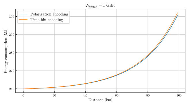
Figure 18: Energy required to distill 1Gbit of secret key using different choices of encoding.

Appendix E Comparison with measured values

As explained with Table 3, some values for the energy consumption of the hardware elements used in this study have been measured directly in a lab. In Figure 19, the difference on the energy required to distill 1 Gbit of secret key using the three DV-QKD protocols studied in this work is shown when using both the measured values and the theoretical values. Since the measured values are almost always lower than the theoretical ones, the overall energy consumption is also lower, as expected. This is coherent with the fact that hardware manuals give an upper bound on the energy consumption. The real consumption of protocols is thus lower than the predictions, although the order of magnitude remains correct.

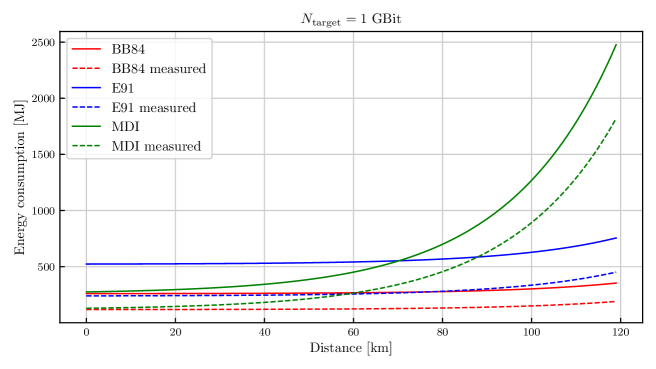
Figure 19: Comparison between the theoretical (plain lines) and the measured (dashed lines) values of the energy required to distill 1 Gbit of secret key using the three DV-QKD protocols.

Appendix F Distribution of power consumption

In Figure 20, the distribution of power usage between components for the studied QKD protocols (BB84, E91, MDI and CV) is plotted as a pie charts, using shades of blue for the source and shades of orange for the detection.

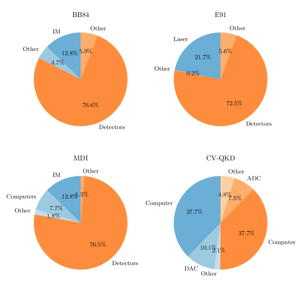
Figure 20: Distribution of power consumption for the different QKD protocols. Shades of blue are used for the source components and shades of orange for the detection components. A darker color indicates a higher power contribution.

Clearly, the biggest contribution for the DV protocols is the detection with the SNSPDs occupying around $75\%$ of the power consumption. For E91, the laser is then the second biggest source of energy consumption, which is due to the high energy required for the generation of photon pairs through non-linear effects. For CV-QKD, the distribution between Alice and Bob is almost equal with the biggest contribution coming from the computers and then from the DAC and ADC.

IEEEtran biblio

References

- [1] S. Wehner, D. Elkouss, and R. Hanson, “Quantum internet: A vision for the road ahead,” Science, vol. 362, no. 6412, 2018. [Online]. Available: https://science.sciencemag.org/content/362/6412/eaam9288
- [2] V. Martin, J. P. Brito, L. Ortiz, R. B. Mendez, J. S. Buruaga, R. J. Vicente, A. Sebastián-Lombraña, D. Rincon, F. Perez, C. Sanchez, M. Peev, H. H. Brunner, F. Fung, A. Poppe, F. Fröwis, A. J. Shields, R. I. Woodward, H. Griesser, S. Roehrich, F. D. L. Iglesia, C. Abellan, M. Hentschel, J. M. Rivas-Moscoso, A. Pastor, J. Folgueira, and D. R. Lopez, “Madqci: a heterogeneous and scalable sdn qkd network deployed in production facilities,” 2023. [Online]. Available: https://arxiv.org/abs/2311.12791
- [3] F. Wissel, O. Nikiforov, D. Giemsa, and M. Gunkel, “The opportunities and challenges of euroqci,” in 2024 Optical Fiber Communications Conference and Exhibition (OFC), 2024, pp. 1–3.
- [4] A. Auffèves, “Quantum technologies need a quantum energy initiative,” PRX Quantum, vol. 3, p. 020101, Jun 2022. [Online]. Available: https://link.aps.org/doi/10.1103/PRXQuantum.3.020101
- [5] M. Fellous-Asiani, J. H. Chai, Y. Thonnart, H. K. Ng, R. S. Whitney, and A. Auffèves, “Optimizing resource efficiencies for scalable full-stack quantum computers,” PRX Quantum, vol. 4, p. 040319, Oct 2023. [Online]. Available: https://link.aps.org/doi/10.1103/PRXQuantum.4.040319
- [6] F. Meier and H. Yamasaki, “Energy-consumption advantage of quantum computation,” 2023. [Online]. Available: https://arxiv.org/abs/2305.11212
- [7] I. Q. I. R. Group, “Architectural principles for a quantum internet, https://datatracker.ietf.org/doc/draft-irtf-qirg-principles/.” [Online]. Available: https://datatracker.ietf.org/doc/draft-irtf-qirg-principles/
- [8] M. Bozzio, U. Chabaud, I. Kerenidis, and E. Diamanti, “Quantum weak coin flipping with a single photon,” 2020.
- [9] G. Demay and U. Maurer, “Unfair coin tossing,” 2013 IEEE International Symposium on Information Theory, pp. 1556–1560, 2013.
- [10] A. Unnikrishnan, I. MacFarlane, R. Yi, E. Diamanti, D. Markham, and I. Kerenidis, “Anonymity for practical quantum networks,” Physical Review Letters, vol. 122, 11 2018.
- [11] M. Bozzio, A. Orieux, L. Trigo Vidarte, I. Zaquine, I. Kerenidis, and E. Diamanti, “Experimental investigation of practical unforgeable quantum money,” npj Quantum Information, vol. 4, no. 1, Jan 2018. [Online]. Available: http://dx.doi.org/10.1038/s41534-018-0058-2
- [12] F. Centrone, E. Diamanti, and I. Kerenidis, “Practical quantum electronic voting,” Phys. Rev. Applied, vol. 18, p. 014005, 2022.
- [13] F. Centrone, F. Grosshans, and V. Parigi, “Cost and routing of continuous-variable quantum networks,” Physical Review A, vol. 108, no. 4, p. 042615, 2023.
- [14] C. H. Bennett and G. Brassard, “Quantum Cryptography: Public Key Distribution and Coin Tossing,” in Proceedings of the IEEE International Conference on Computers, Systems and Signal Processing. Bangalore, India, December 1984: IEEE Computer Society Press, New York, 1984, pp. 175–179.
- [15] ——, “Quantum cryptography: Public key distribution and coin tossing,” Theoretical Computer Science, vol. 560, pp. 7–11, 2014, theoretical Aspects of Quantum Cryptography – celebrating 30 years of BB84. [Online]. Available: https://www.sciencedirect.com/science/article/pii/S0304397514004241
- [16] H.-K. Lo and J. Preskill, “Security of quantum key distribution using weak coherent states with nonrandom phases,” Quantum Info. Comput., vol. 7, no. 5, p. 431–458, Jul. 2007.
- [17] A. K. Ekert, “Quantum cryptography based on bell’s theorem,” Phys. Rev. Lett., vol. 67, pp. 661–663, Aug 1991. [Online]. Available: https://link.aps.org/doi/10.1103/PhysRevLett.67.661
- [18] C. H. Bennett, G. Brassard, and N. D. Mermin, “Quantum cryptography without bell’s theorem,” Phys. Rev. Lett., vol. 68, pp. 557–559, Feb 1992. [Online]. Available: https://link.aps.org/doi/10.1103/PhysRevLett.68.557
- [19] V. Makarov, A. Anisimov, and J. Skaar, “Effects of detector efficiency mismatch on security of quantum cryptosystems,” Phys. Rev. A, vol. 74, p. 022313, Aug 2006. [Online]. Available: https://link.aps.org/doi/10.1103/PhysRevA.74.022313
- [20] L. Lydersen, C. Wiechers, C. Wittmann, D. Elser, J. Skaar, and V. Makarov, “Hacking commercial quantum cryptography systems by tailored bright illumination,” Nature Photonics - NAT PHOTONICS, vol. 4, 08 2010.
- [21] M. Lucamarini, Z. Yuan, J. F. Dynes, and A. J. Shields, “Overcoming the rate–distance limit of quantum key distribution without quantum repeaters,” Nature, vol. 557, no. 7705, p. 400–403, May 2018. [Online]. Available: http://dx.doi.org/10.1038/s41586-018-0066-6
- [22] J.-P. Chen, C. Zhang, Y. Liu, C. Jiang, W.-J. Zhang, Z.-Y. Han, S.-Z. Ma, X.-L. Hu, Y.-H. Li, H. Liu, F. Zhou, H.-F. Jiang, T.-Y. Chen, H. Li, L.-X. You, Z. Wang, X.-B. Wang, Q. Zhang, and J.-W. Pan, “Twin-field quantum key distribution over 511 km optical fiber linking two distant metropolitan areas,” Nature Photon., vol. 15, pp. 570–575, 2021.
- [23] Y. Zhang, Y. Bian, Z. Li, S. Yu, and H. Guo, “Continuous-variable quantum key distribution system: past, present, and future,” 2024.
- [24] F. Grosshans and P. Grangier, “Continuous variable quantum cryptography using coherent states,” Physical review letters, vol. 88, no. 5, p. 057902, 2002.
- [25] S. Ghorai, P. Grangier, E. Diamanti, and A. Leverrier, “Asymptotic security of continuous-variable quantum key distribution with a discrete modulation,” Physical Review X, vol. 9, no. 2, p. 021059, 2019.
- [26] A. Denys, P. Brown, and A. Leverrier, “Explicit asymptotic secret key rate of continuous-variable quantum key distribution with an arbitrary modulation,” Quantum, vol. 5, p. 540, 2021.
- [27] E. Björnson and E. G. Larsson, “How energy-efficient can a wireless communication system become?” in 2018 52nd Asilomar Conference on Signals, Systems, and Computers, 2018, pp. 1252–1256.
- [28] R. Yehia, Y. Pietri, and C. Pascual Garcia, “Github repository for the simulation modules, https://github.com/rajayehia/qenergy/tree/main.” [Online]. Available: https://github.com/RajaYehia/QEnergy/tree/main
- [29] Y. Piétri, L. T. Vidarte, M. Schiavon, L. Vivien, P. Grangier, A. Rhouni, and E. Diamanti, “Experimental demonstration of continuous-variable quantum key distribution with a silicon photonics integrated receiver,” 2023. [Online]. Available: https://arxiv.org/abs/2311.03978
- [30] C. Bruynsteen, M. Vanhoecke, J. Bauwelinck, and X. Yin, “Integrated balanced homodyne photonic–electronic detector for beyond 20 ghz shot-noise-limited measurements,” Optica, vol. 8, no. 9, pp. 1146–1152, Sep 2021. [Online]. Available: https://opg.optica.org/optica/abstract.cfm?URI=optica-8-9-1146
- [31] Y. Piétri, M. Schiavon, V. M. Acosta, B. Gouraud, L. T. Vidarte, P. Grangier, A. Rhouni, and E. Diamanti, “Qosst: A highly-modular open source platform for experimental continuous-variable quantum key distribution,” 2024.
- [32] F. Roumestan, A. Ghazisaeidi, J. Renaudier, L. T. Vidarte, E. Diamanti, and P. Grangier, “High-rate continuous variable quantum key distribution based on probabilistically shaped 64 and 256-qam,” 2021. [Online]. Available: https://arxiv.org/abs/2111.12356
- [33] N. Jain, H.-M. Chin, H. Mani, C. Lupo, D. S. Nikolic, A. Kordts, S. Pirandola, T. B. Pedersen, M. Kolb, B. Ömer, C. Pacher, T. Gehring, and U. L. Andersen, “Practical continuous-variable quantum key distribution with composable security,” Nature Communications, vol. 13, no. 1, p. 4740, Aug 2022. [Online]. Available: https://doi.org/10.1038/s41467-022-32161-y
- [34] M. Navascués, E. Wolfe, D. Rosset, and A. Pozas-Kerstjens, “Genuine network multipartite entanglement,” Physical Review Letters, vol. 125, no. 24, Dec 2020. [Online]. Available: http://dx.doi.org/10.1103/PhysRevLett.125.240505
- [35] D. M. Greenberger, M. A. Horne, and A. Zeilinger, Going Beyond Bell’s Theorem. Dordrecht: Springer Netherlands, 1989, pp. 69–72. [Online]. Available: https://doi.org/10.1007/978-94-017-0849-4_10
- [36] F. Hahn, J. de Jong, and A. Pappa, “Anonymous quantum conference key agreement,” PRX Quantum, vol. 1, no. 2, Dec 2020. [Online]. Available: http://dx.doi.org/10.1103/PRXQuantum.1.020325
- [37] G. Murta, F. Grasselli, H. Kampermann, and D. Bruß, “Quantum conference key agreement: A review,” Advanced Quantum Technologies, vol. 3, no. 11, p. 2000025, Sep 2020. [Online]. Available: http://dx.doi.org/10.1002/qute.202000025
- [38] M. Epping, H. Kampermann, C. macchiavello, and D. Bruß, “Multi-partite entanglement can speed up quantum key distribution in networks,” New Journal of Physics, vol. 19, no. 9, p. 093012, sep 2017. [Online]. Available: https://dx.doi.org/10.1088/1367-2630/aa8487
- [39] M. Proietti, J. Ho, F. Grasselli, P. Barrow, M. Malik, and A. Fedrizzi, “Experimental quantum conference key agreement,” Science Advances, vol. 7, no. 23, p. eabe0395, 2021. [Online]. Available: https://www.science.org/doi/abs/10.1126/sciadv.abe0395
- [40] C. Ottaviani, C. Lupo, R. Laurenza, and S. Pirandola, “Modular network for high-rate quantum conferencing,” Communications Physics, vol. 2, no. 1, p. 118, Sep. 2019. [Online]. Available: https://www.nature.com/articles/s42005-019-0209-6
- [41] N. Maring, A. Fyrillas, M. Pont, E. Ivanov, P. Stepanov, N. Margaria, W. Hease, A. Pishchagin, T. H. Au, S. Boissier, E. Bertasi, A. Baert, M. Valdivia, M. Billard, O. Acar, A. Brieussel, R. Mezher, S. C. Wein, A. Salavrakos, P. Sinnott, D. A. Fioretto, P.-E. Emeriau, N. Belabas, S. Mansfield, P. Senellart, J. Senellart, and N. Somaschi, “A general-purpose single-photon-based quantum computing platform,” Nature Photonics, vol. 18, 2024. [Online]. Available: https://doi.org/10.1038/s41566-024-01403-4
- [42] Y. Dodis and D. Wichs, “Non-malleable extractors and symmetric key cryptography from weak secrets,” in Proceedings of the Forty-First Annual ACM Symposium on Theory of Computing, ser. STOC ’09. New York, NY, USA: Association for Computing Machinery, 2009, p. 601–610. [Online]. Available: https://doi.org/10.1145/1536414.1536496
- [43] B. Dowling, T. B. Hansen, and K. G. Paterson, “Many a mickle makes a muckle: A framework for provably quantum-secure hybrid key exchange,” in Post-Quantum Cryptography, J. Ding and J.-P. Tillich, Eds. Cham: Springer International Publishing, 2020, pp. 483–502.
- [44] M. Gast, 802.11 wireless networks: the definitive guide. ” O’Reilly Media, Inc.”, 2005.
- [45] S. L. Braunstein and P. Van Loock, “Quantum information with continuous variables,” Reviews of modern physics, vol. 77, no. 2, p. 513, 2005.
- [46] Y. Zhang, Y. Bian, Z. Li, S. Yu, and H. Guo, “Continuous-variable quantum key distribution system: Past, present, and future,” Applied Physics Reviews, vol. 11, no. 1, p. 011318, 03 2024. [Online]. Available: https://doi.org/10.1063/5.0179566
- [47] C. L. Cortes, P. Lefebvre, N. Lauk, M. J. Davis, N. Sinclair, S. K. Gray, and D. Oblak, “Sample-efficient adaptive calibration of quantum networks using bayesian optimization,” Phys. Rev. Appl., vol. 17, p. 034067, Mar 2022. [Online]. Available: https://link.aps.org/doi/10.1103/PhysRevApplied.17.034067
- [48] Y.-P. Huang, J. B. Altepeter, and P. Kumar, “Optimized heralding schemes for single photons,” Phys. Rev. A, vol. 84, p. 033844, Sep 2011. [Online]. Available: https://link.aps.org/doi/10.1103/PhysRevA.84.033844
- [49] K. Kikuchi, “Fundamentals of coherent optical fiber communications,” Journal of Lightwave Technology, vol. 34, pp. 157–179, 1 2016. [Online]. Available: http://dx.doi.org/10.1109/jlt.2015.2463719
- [50] D. E. Browne and T. Rudolph, “Resource-efficient linear optical quantum computation,” Physical Review Letters, vol. 95, no. 1, Jun. 2005. [Online]. Available: http://dx.doi.org/10.1103/PhysRevLett.95.010501
- [51] H. Cao, L. Hansen, F. Giorgino, L. Carosini, P. Zahálka, F. Zilk, J. Loredo, and P. Walther, “Photonic source of heralded greenberger-horne-zeilinger states,” Physical Review Letters, vol. 132, no. 13, Mar. 2024. [Online]. Available: http://dx.doi.org/10.1103/PhysRevLett.132.130604
- [52] S. de Bone, R. Ouyang, K. Goodenough, and D. Elkouss, “Protocols for creating and distilling multipartite ghz states with bell pairs,” IEEE Transactions on Quantum Engineering, vol. 1, pp. 1–10, 2020.
- [53] H.-S. Zhong, Y. Li, W. Li, L.-C. Peng, Z.-E. Su, Y. Hu, Y.-M. He, X. Ding, W. Zhang, H. Li, L. Zhang, Z. Wang, L. You, X.-L. Wang, X. Jiang, L. Li, Y.-A. Chen, N.-L. Liu, C.-Y. Lu, and J.-W. Pan, “12-photon entanglement and scalable scattershot boson sampling with optimal entangled-photon pairs from parametric down-conversion,” Phys. Rev. Lett., vol. 121, p. 250505, Dec 2018. [Online]. Available: https://link.aps.org/doi/10.1103/PhysRevLett.121.250505
- [54] S. Bartolucci, P. Birchall, H. Bombin, H. Cable, C. Dawson, M. Gimeno-Segovia, E. Johnston, K. Kieling, N. Nickerson, M. Pant, F. Pastawski, T. Rudolph, and C. Sparrow, “Fusion-based quantum computation,” Nature Communications, vol. 14, 2023. [Online]. Available: https://doi.org/10.1038/s41467-023-36493-1
- [55] A. Olivo and F. Grosshans, “Ancilla-assisted linear optical bell measurements and their optimality,” Phys. Rev. A, vol. 98, p. 042323, 09 2018. [Online]. Available: https://link.aps.org/doi/10.1103/PhysRevA.98.042323
- [56] M. J. Bayerbach, S. E. D’Aurelio, P. van Loock, and S. Barz, “Bell-state measurement exceeding 50% success probability with linear optics,” Science Advances, vol. 9, no. 32, 08 2023. [Online]. Available: http://dx.doi.org/10.1126/sciadv.adf4080
- [57] H.-K. Lo, M. Curty, and B. Qi, “Measurement-device-independent quantum key distribution,” Physical Review Letters, vol. 108, no. 13, Mar 2012. [Online]. Available: http://dx.doi.org/10.1103/PhysRevLett.108.130503
- [58] P. W. Shor and J. Preskill, “Simple proof of security of the bb84 quantum key distribution protocol,” Physical review letters, vol. 85, no. 2, p. 441, 2000.
- [59] V. Scarani, H. Bechmann-Pasquinucci, N. J. Cerf, M. Dušek, N. Lütkenhaus, and M. Peev, “The security of practical quantum key distribution,” Rev. Mod. Phys., vol. 81, pp. 1301–1350, Sep 2009. [Online]. Available: https://link.aps.org/doi/10.1103/RevModPhys.81.1301
- [60] S. Watanabe, R. Matsumoto, T. Uyematsu, and Y. Kawano, “Key rate of quantum key distribution with hashed two-way classical communication,” Physical Review A, vol. 76, no. 3, Sep. 2007. [Online]. Available: http://dx.doi.org/10.1103/PhysRevA.76.032312
- [61] E. Diamanti and A. Leverrier, “Distributing secret keys with quantum continuous variables: principle, security and implementations,” Entropy, vol. 17, no. 9, pp. 6072–6092, 2015.
- [62] F. Roumestan, A. Ghazisaeidi, J. Renaudier, L. T. Vidarte, A. Leverrier, E. Diamanti, and P. Grangier, “Experimental demonstration of discrete modulation formats for continuous variable quantum key distribution,” 2022.
- [63] S. Fossier, E. Diamanti, T. Debuisschert, R. Tualle-Brouri, and P. Grangier, “Improvement of continuous-variable quantum key distribution systems by using optical preamplifiers,” Journal of Physics B: Atomic, Molecular and Optical Physics, vol. 42, no. 11, p. 114014, may 2009. [Online]. Available: https://dx.doi.org/10.1088/0953-4075/42/11/114014
- [64] I. Devetak and A. Winter, “Distillation of secret key and entanglement from quantum states,” Proceedings of the Royal Society A: Mathematical, Physical and engineering sciences, vol. 461, no. 2053, pp. 207–235, 2005.
IEEEtran \bibliographyHbiblio