Vecchia Gaussian Processes: Probabilistic Properties, Minimax Rates and Methodological Developments

Botond Szabo label=e1]botond.szabo@unibocconi.it [    Yichen Zhulabel=e2]yichen.zhu@unibocconi.it [ Bocconi Institute for Data Science and Analytics, Bocconi University presep= , ]e1,e2    Botond Szabo label=e1]botond.szabo@unibocconi.it [    Yichen Zhulabel=e2]yichen.zhu@unibocconi.it [ Bocconi Institute for Data Science and Analytics, Bocconi University presep= , ]e1,e2

Supplementary Materials to “Vecchia Gaussian Processes: Probabilistic Properties, Minimax Rates and Methodological Developments”

Botond Szabo label=e1]botond.szabo@unibocconi.it [    Yichen Zhulabel=e2]yichen.zhu@unibocconi.it [ Bocconi Institute for Data Science and Analytics, Bocconi University presep= , ]e1,e2    Botond Szabo label=e1]botond.szabo@unibocconi.it [    Yichen Zhulabel=e2]yichen.zhu@unibocconi.it [ Bocconi Institute for Data Science and Analytics, Bocconi University presep= , ]e1,e2
Abstract

Gaussian Processes (GPs) are widely used to model dependency in spatial statistics and machine learning, yet the exact computation suffers an intractable time complexity of $O(n^{3})$. Vecchia approximation allows scalable Bayesian inference of GPs in $O(n)$ time by introducing sparsity in the spatial dependency structure that is characterized by a directed acyclic graph (DAG). Despite the popularity in practice, it is still unclear how to choose the DAG structure and there are still no theoretical guarantees in nonparametric settings. In this paper, we systematically study the Vecchia GPs as standalone stochastic processes and uncover important probabilistic properties and statistical results in methodology and theory. For probabilistic properties, we prove that the conditional distributions of the Matérn GPs, as well as the Vecchia approximations of the Matérn GPs, can be characterized by polynomials. This allows us to prove a series of results regarding the small ball probabilities and RKHSs of Vecchia GPs. For statistical methodology, we provide a principled guideline to choose parent sets as norming sets with fixed cardinality and provide detailed algorithms following such guidelines. For statistical theory, we prove posterior contraction rates for applying Vecchia GPs to regression problems, where minimax optimality is achieved by optimally tuned GPs via either oracle rescaling or hierarchical Bayesian methods. Our theory and methodology are demonstrated with numerical studies, where we also provide efficient implementation of our methods in C++ with R interfaces.

62G08,
60G15, 62H11,
Gaussian Process,
Minimax Rate,
Norming Set,
Vecchia Approximation,
keywords:
[class=MSC]
keywords:
\startlocaldefs\endlocaldefs

and

1 Introduction

1.1 Background and Related Work

Gaussian processes have seen a wide range of applications amongst others in spatial statistics (e.g., [20, 11, 19]), machine learning (e.g., [55, 35, 39]) and epidemiology [6] due to their flexibility in characterizing dependency structures and convenience for uncertainty quantification. However, the exact statistical inference for GPs in various methods, ranging from maximal likelihood estimation of GP parameters to posterior inference based on GP priors, suffers the $O(n^{3})$ computational complexity due to the need to compute the determinant and inverse of the $n\times n$ covariance matrix. There has been a substantial amount of research effort to circumvent this computational problem, including but not limited to inducing variable or reduced rank approximations [43, 10, 4, 50], covariance tapering [16, 29, 47], compositional likelihoods [2, 5], distributed methods [14, 13, 49] and last but not the least, Vecchia approximations. Vecchia approximations of Gaussian processes (Vecchia GPs) was named after the author of [53] and are defined as follows. For a joint density decomposed into a sequence of univariate conditional densities,

$$p(Z_{\mathcal{X}_{n}})=p(Z_{X_{1}})\prod_{i=2}^{n}p(Z_{X_{i}}|Z_{X_{1}},Z_{X_{2}},\cdots,Z_{X_{i-1}}),$$

Vecchia approximations replace each conditional set with a smaller set, known as the parent set, to approximate the joint density:

$$p(Z_{\mathcal{X}_{n}})\approx p(Z_{X_{1}})\prod_{i=2}^{n}p(Z_{X_{i}}|Z_{\mathrm{pa}(X_{i})}).$$

Applying the above approximation to a collection of finite dimensional marginals of a GP results in, under weak assumptions, a new GP111For a proof, refer to [12] or [56], called the Vecchia GP. The approximated GP is referred to as the mother Gaussian process. The underlying conditional dependence structure in the approximation, i.e. the set of parents for each covariate, is summarized by a DAG.

There is an extensive literature about Vecchia approximations of GPs (e.g., [12, 28, 27, 42, 9]). The popularity of Vecchia GPs can be mostly attributed to its two practical advantages. First, under the condition that all parent sets have bounded cardinality, Vecchia approximations possess $O(n)$ computational complexity for evaluating the joint density. This renders Veccha GPs as one of the best scalable methods for GP approximations. Second, the Vecchia approximation of a GP is not just an approximation of the mother GP, but also a valid GP itself. This brings immense flexibility for the practical application of Vecchia GPs in the sense that the estimates related to Vecchia GPs are statistically meaningful regardless whether the approximations are good or not.

Despite its success in applications and popularity amongst researchers, there are major methodological and theoretical challenges that hinder the further developments of Vecchia GPs. Methodologically, the optimal choice of the DAG structure is not entirely clear, despite playing a vital role in the empirical performance of Vecchia GPs. In fact, several of the proposed concepts even contradict each other. For example, many papers propose to choose close neighbors for parent sets [12, 57], while other authors promote remote locations [3] or random ordering [24]. Moreover, it is often claimed that larger parent sets lead to better performance for Vecchia GPs. Furthermore, the only qualitative result regarding cardinality of parent sets are of poly-log order [44, 26, 57], and it is not clear if further increasing the cardinality would indeed bring non-marginal statistical advantages. We summarize the above challenges in the following two research questions:

  • Q1 What is the minimal cardinality of the parent sets in the Vecchia GP to achieve optimal performance?

  • Q2 How shall the parent sets be chosen to reach optimal performance?

We answer these two questions from a mathematical statistics perspective. We show that optimally tuned Vecchia GPs achieve optimal statistical inference in a minimax sense. More concretely, we investigate the posterior contraction rates of Vecchia GPs and show that the minimax rates can be achieved for suitably chosen DAG structures and optimally tuned mother GPs. Despite the great popularity of Vecchia GPs in practice, their theoretical understanding were so far rather limited. In fact, we are only aware of the following few, recent works studying its theoretical properties. Specifically, in the univariate case under some assumptions on the variance, [56] derives the asymptotic normality of the Vecchia GPs. Under various conditions about the DAG structures, covariance functions and the datasets, [44] shows the precision matrices of Vecchia GPs approximate well the precision matrices of the mother GPs, [57] shows that the Vecchia GPs approximate well the mother GPs in Wasserstein distance. Furthermore, [26] shows that the maximal likelihood estimation for GP parameters of Vecchia GPs has the same convergence and asymptotic normality properties as the mother GPs.

Although all the above works offer solid contributions to the literature of Vecchia GPs, none of them directly addresses the question of posterior consistency around the truth in nonparametric models. In fact, all previous works tackle the theory of Vecchia GPs from the perspective of “approximation”. They either directly quantify the approximation error between Vecchia GPs and the corresponding mother GPs, or study the statistical properties of the Vecchia GPs based on the approximation error bounds between the Vecchia GPs and their corresponding mother GPs. However, such strategy might lead to sub-optimal results. Vecchia GPs are well-defined Gaussian processes themselves. Their properties, both empirical and theoretical, shall be studied as standalone problems that do not require good approximations to their mother GPs as prerequisites. After all, the main goal is to provide a scalable process with similarly good statistical properties as the original GP. Restricting ourselves to an overly accurate approximation of the mother GP prevents us to fully explore the computational advantages offered by the Vecchia approach.

To investigate the statistical aspects of Vecchia GPs one has to first understand its probabilistic properties, which so far were barely studied. More generally, GPs are typically defined through their marginal distributions and the standard probabilistic techniques are tailored to such perspective, see [30, 37, 1]. However, Vecchia GPs are defined through the conditional distributions encoded in a DAG structure. For such constructions, to the best of our knowledge, there are no general tools derived to compute the small ball probabilities and other probabilistic aspects of the process. Hence, one of the main challenge of our work was to derive new mathematical techniques for studying the probabilistic properties of Vecchia approximated GPs. To highlight that the mother and Vecchia GPs can have substantially different properties, we note that in case of the popular Matérn process the mother GP is stationary while the Vecchia GP is not. In fact, little is known about the covariance kernel of the Vecchia GP or the Reproducing Kernel Hilbert Space (RKHS) associated to the process. Therefore, the techniques used for isotropic covariance functions, like the Matérn kernel, relying on spectral densities and RKHSs do not apply in case of Vecchia approximations.

1.2 Our Contributions

In this section, we discuss our contributions to literature of Vecchia GPs from the perspectives of probabilistic properties, statistical theory and methodological developments, as well as the connections among them.

1.2.1 Probabilistic Properties

Our contributions to the probabilistic properties of Vecchia GPs are twofold. First, we systematically study the conditional distributions that define the Vecchia GPs. We show that the conditional expectations of the Vecchia GPs can asymptotically be characterized with local polynomial interpolations. Furthermore, we prove that the conditional variances coincide with the error rates of these local polynomial approximations. Moreover, under suitable DAG structures, the degree of these local polynomials is exactly $\underline{\alpha}$, the largest integer strictly smaller than $\alpha$. While the limit of Gaussian interpolation has been studied in the literature of radial basis functions [15, 33, 46, 36], to the best of our knowledge, we are the first to prove the stronger version with uniform convergence rate and to make this connection to the Vecchia GPs. On the other hand, the characterization of the asymptotic properties of the variance is an entirely novel contribution.

Our second contribution is the derivation of various probabilistic properties of Vecchia GPs based on the conditional probabilities instead of the standard route through marginal probabilities. One important quantity is the small deviation bound (i.e. small ball probability) of the GP, which is typically derived by its relation to the entropy of the unit ball of the associated RKHS [30, 37, 1, 22]. However, for Vecchia GPs the properties of the associated RKHS are not well charaterized. In our work we provide a new set of tools, tailored to Vecchia GPs, but may be useful for other types of processes as well.

1.2.2 Nonparametric Theory

Built upon the probabilistic properties discussed above, in context of the nonparametric regression model, we prove that the posteriors arising from optimally tuned (i.e. scaled) Vecchia GPs attain the minimax contraction rate for Hölder smooth functions. This demonstrates that Vecchia GPs reduce the computational costs of their mother GPs considerably without sacrificing statistical efficiency. The optimal choice of the tuning/scaling parameter depends on the smoothness of the underlying functional parameter of interest, which is typically not available in practice. Therefore, we consider a data driven tuning of the GP, by endowing the scaling parameter with another layer of prior, forming a two-level, so called hierarchical prior distribution. We show that such hierarchical Vecchia GPs under mild assumptions, concentrate their masses around the true functional parameter with the minimax adaptive rate.

1.2.3 Methodological Developments

Our research was partially motivated by the methodological Questions Q1 and Q2 that remained unclear for a long time. We answer these questions from a mathematical statistics perspective, focusing on optimal recovery of the underlying true signal of interest in context of the nonparametric regression model. We show, that well chosen parent sets with cardinality equal to ${\underline{\alpha}+d\choose\underline{\alpha}}$ is sufficient and necessary to achieve minimax contraction rate with the Vecchia approximation. More concretely, one has to choose a norming set as parents with a fixed, universal norming constant. For (approximately) grid data, we provide an explicit formulation of such sets, while for more general datasets we propose algorithms that can potentially find such norming sets given they exist. Numerical studies in Section 6 demonstrate that our method achieves almost identity performance in nonparametric function estimation comparing to state-of-the-art methods, while having $75\%$ reduction in computational time.

Our perspective and hence our answers to questions Q1 and Q2 are different from the bulk of the literature on Vecchia GPs. We believe that these differences reveal hidden features and characteristics and therefore contributes significantly to the understanding of this popular, but so far theoretically not well underpinned method. In Section 7 we provide a detailed discussion of our results and their implications. Here we focus on one of the most important methodological aspect, i.e. the cardinality of the parents sets. The results in [44], [57] and [26] all require the parent sets to grow at poly-log rate in $n$, while we only need fixed sized parent sets. There is, however, no contradictions here. Previous works typically consider Vecchia GP approximations to the mother GPs and the poly-log size ensures vanishing approximation error. In contrast, we directly investigate the properties of the posterior resulting from the Vecchia GP as standalone prior and derive contraction rates in a nonparametric framework. Bypassing the approximation step, one can typically end up with weaker conditions.

1.3 Notations

We introduce some notations used throughout the paper. For easier readability we organized them into subsections.

1.3.1 Gaussian Processes

Let $\mathcal{X}\subset\mathbb{R}^{d}$ be the domain of the centered mother GPs $(Z_{x},x\in\mathcal{X})$ with covariance kernel $K(\cdot,\cdot):\mathcal{X}\times\mathcal{X}\to\mathbb{R}$. We focus on the Matérn covariance function (Section 4.2.1 of [45]) with regularity hyper-parameter $\alpha>0$:

$$K(x_{1},x_{2})=\frac{2^{1-\alpha}}{\Gamma(\alpha)}\|x_{1}-x_{2}\|_{2}^{\alpha}\mathcal{K}_{\alpha}\left(\|x_{1}-x_{2}\|_{2}\right),$$ (1)

where $\mathcal{K}_{\alpha}$ denotes the modified Bessel function of the second kind with parameter $\alpha$. It has a simple characterization in terms of Fourier transform

$$K(x_{1},x_{2})\propto\int_{\mathbb{R}^{d}}e^{-\iota\langle x_{1}-x_{2},\xi\rangle}(1+\|\xi\|_{2}^{2})^{-\alpha-d/2}d\xi,$$ (2)

where the constant in “$\propto$” only dependends on $\alpha$ and $d$, see equation (11.4) of [22]. For $s,\tau>0$, the rescaled GP $(Z_{x}^{\tau,s},x\in\mathcal{X})$ is defined as

$$Z^{\tau,s}_{x}=sZ_{\tau x},\;\;\forall x\in\tau^{-1}\mathcal{X}.$$

We will refer to $\tau$ as time, while to $s$ as space (re-)scaling hyper-parameters.

Let us denote by $(\hat{Z}_{x}^{\tau,s},x\in\mathcal{X})$ the Vecchia approximation of the mother GP $(Z^{\tau,s}_{x},x\in\mathcal{X})$. When $\tau=s=1$, we abbreviate the notation as $(\hat{Z}_{x},x\in\mathcal{X})$ and let $\hat{K}(\cdot,\cdot):\mathcal{X}\times\mathcal{X}\to\mathbb{R}$ denote the corresponding covariance kernel which is typically different from the mother covariance kernel $K(\cdot,\cdot)$. For arbitrary scaling parameters $\tau,s>0$ let $K^{\tau,s}(\cdot,\cdot)$ and $\hat{K}^{\tau,s}(\cdot,\cdot)$ denote the covariance functions of the corresponding rescaled processes. For simplicity of notations, we abbreviate the process $(Z^{\tau,s}_{x},x\in\mathcal{X})$ as $Z^{\tau,s}$. Similarly let us introduce the abbreviations $\hat{Z}^{\tau,s}$, $Z$ and $\hat{Z}$. Furthermore, let $\mathbb{H}$ and $\mathbb{H}^{\tau,s}$ denote the RKHSs associated with the mother GPs $Z$ and $Z^{\tau,s}$, respectively. Similarly, let $\mathbb{H}_{n}$ and $\mathbb{H}_{n}^{\tau,s}$ be the RKHSs for the $n$-dimensional marginals of the processes $\hat{Z}_{n}$ and $\hat{Z}^{\tau,s}_{n}$, respectively.

For an arbitrary covariance function $K(\cdot,\cdot):\mathbb{R}^{d}\times\mathbb{R}^{d}\to\mathbb{R}$, and multi indexes $k_{1},k_{2}\in\mathbb{N}^{d}$, let us denote by $K^{(k_{1},k_{2})}(x_{1},x_{2})=\frac{\partial^{k_{1}}}{\partial x_{1}^{k_{1}}}\frac{\partial^{k_{2}}}{\partial x_{2}^{k_{2}}}K(x_{1},x_{2})$ the $k_{1}$th and $k_{2}$the order derivatives with respect to the first and second arguments, respectively. Furthermore, for all finite sets $A,B\subset\mathcal{X}$, we denote the covariance matrix between $A$ and $B$ under the covariance function $K(\cdot,\cdot)$ as $K_{A,B}$. If $B=\{x\}$ contains a single element, we slightly abuse the notation by writing $K_{A,x}=K_{A,\{x\}}$.

1.3.2 Ordering and Indices

For a $d$-dimensional vector $x\in\mathbb{R}^{d}$, we denote its coordinates as

$$x=(x[1],x[2],\cdots,x[d])^{T}.$$ (3)

Similarly, $M[i,j]$ denotes the cell in the $i$th row and $j$th column of the matrix $M$. Furthermore, for multi-index $k=(k[1],k[2],\cdots,k[d])^{T}\in\mathbb{N}^{d}$, we use the convention $|k|=\sum_{j=1}^{d}k[j]$.

For elements in $\mathbb{R}^{d}$, we define the lexicographical ordering “$\prec$” as follow: for all $x=(x[1],x[2],\cdots,x[d])^{T}$ and $y=(y[1],y[2],\cdots,y[d])^{T}$, we say $x\prec y$ if either $\sum_{i}x[i]<\sum_{i}y[i]$ or $\sum_{i}x[i]=\sum_{i}y[i]$ and there exists a positive integer $d^{\prime}\leq d$, such that $x[d^{\prime}]<y[d^{\prime}]$ and $x[i]=y[i],\;\forall i\leq d^{\prime}-1$. Let us then denote by $k_{(i)}\in\mathbb{N}^{d}$ the $i$th multi-index in $\mathbb{N}^{d}$ with respect to the lexicographical ordering. Note that the first index is $k_{(1)}=(0,0,\cdots,0)^{T}$.

Finally, let $f:\mathbb{R}^{d}\to\mathbb{R}$ be a $l$th order differentiable function. Then the derivative of $f$ with respect to multi-index $k\in\mathbb{N}^{d}$ at $x\in\mathbb{R}^{d}$ is denoted by

$$f^{(k)}(x)=\prod_{i=1}^{d}\frac{\partial^{k[i]}}{\partial x[i]^{k[i]}}f(x).$$

1.3.3 Sets, Functions and Functionals

For a finite set $A$, let $|A|$ denote its cardinality. For $t>0$, denote by $tA$ the set $\{tx:x\in A\}$.

For a set $\Omega$ as a subset of a field, let $\ell^{p}(\Omega)$ denote the collection of $\ell^{p}$ functions defined on $\Omega$. For a set $\Omega\subset\mathbb{R}^{d}$ and a function $f:\Omega\to\mathbb{R}$, let $\|f\|_{C^{\alpha}}$ denote the Hölder-$\alpha$ norm of $f$ and let $C^{\alpha}(\Omega)_{1}$ be the set of functions on $\Omega$ with Hölder-$\alpha$ norm bounded by $1$. Similarly, let $\|f\|_{W^{\alpha}}$ be the Sobolev-$\alpha$ norm (same as the $\|\cdot\|_{2,2,\alpha}$ norm in Definition C.6 of [22]) of $f$ and let $W^{\alpha}(\Omega)_{1}$ be the unit ball with respect to this norm. If $\Omega$ coincides with the domain $\mathcal{X}$ of the GP, we abbreviate the above two sets as $C^{\alpha}_{1}$ and $W^{\alpha}_{1}$.

For $\mathcal{X}_{n}\subset\mathbb{R}$ a finite set, the supremum norm of a function $f:\mathbb{R}^{d}\to\mathbb{R}$ on $\mathcal{X}_{n}$ is denoted by $\|f\|_{\infty,n}=\sup_{x\in\mathcal{X}_{n}}|f(x)|$. For two sets $\Omega_{1},\Omega_{2}$ , for $p\in(0,+\infty]$ and an operator $M:\ell^{p}(\Omega_{1})\to\ell^{p}(\Omega_{2})$, the $\ell^{p}$ operator norm is defined as $\|M\|_{p}=\sup_{f\in\ell^{p}(\Omega_{1})}\|M(f)\|_{p}/\|f\|_{p}$.

1.3.4 Other Notations

We use $\iota$ to denote imaginary part of a complex number. For $\alpha\in\mathbb{R}$, let $\underline{\alpha}$ be the largest integer strictly smaller than $\alpha$. For two functions $f_{1}(n)$ and $f_{2}(n)$ of the sample size $n$, the notation $f_{1}(n)\lesssim f_{2}(n)$ means that there exists a universal constant $c$, such that $f_{1}(n)\leq cf_{2}(n)$. Let $\mathbbm{1}_{m}$ be a column vector with length $m$ and all elements equal to one.

1.4 Organization of the Paper

The rest of the paper is organized as follows. Section 2 introduces Vecchia approximations of GPs. Section 3 provides some background knowledge about polynomials and subsequently defines the Layered Norming DAG, providing a principled, theory driven choice of the graphical structures. Section 4 presents some probabilistic properties for Matérn processes and the corresponding Vecchia Matérn processes. Building on these probabilistic properties, in Section 5, we prove minimax contraction rates for appropriately scaled Vecchia GPs, both in the oracle and adaptive framework using hierarchical Bayesian approaches. Section 6 proceeds to demonstrate our theoretical findings with a numerical analysis on synthetic data sets. In Section 7, we discuss the implication of our results, while the proofs are deferred to the supplementary materials.

2 Vecchia Approximations of Gaussian Processes

In this section we first describe the Gaussian Process regression model where we have carried out our analysis and then introduce the Vecchia approximation of GPs. We consider Vecchia GPs both with the fixed hyper-parameters and by endowing them with another layer of priors, resulting in a hierarchical Bayesian prior.

2.1 Gaussian Process Regression

Let us assume that we observe $Y_{1},...,Y_{n}$ satisfying

$$Y_{i}=f(X_{i})+\varepsilon_{i},\quad\varepsilon_{i}\overset{\text{i.i.d.}}{\sim}N(0,\sigma^{2}),\quad i=1,...,n$$ (4)

where the covariates $(X_{i})_{1\leq i\leq n}$ are either random of deterministic, belonging to a compact subset $\mathcal{X}\subset\mathbb{R}^{d}$ and $f\in L_{2}(\mathcal{X})$ is the unknown functional parameter of interest. Let us denote by $\mathcal{D}_{n}=\{(X_{i},Y_{i})_{1\leq i\leq n}\}$ our data. We focus here on the Bayesian Gaussian process regression framework, by endowing $f$ with a GP prior, i.e.

$$f\sim(Z^{\tau,s}_{x},x\in\mathcal{X}),$$ (5)

where $Z^{\tau,s}$ is a GP with rescaling parameters $(\tau,s)$.

The posterior distribution of the regression function given the data, i.e. $f|\mathcal{D}_{n}$, serves as a probabilistic solution to the regression problem. If the hyper-parameters $\tau,s$ and other tuning parameters of the Gaussian process are fixed, the prior is conjugate and the posterior is also a Gaussian process. However, in practice, it is usually difficult to directly choose these hyper-parameters. Therefore, researchers often let the data decide about the optimal choice by endowing them with another layer of prior 222There may exist other parameters for the process $Z^{\tau,s}_{x}$ other than $(\tau,s)$, for example smoothness $\alpha$ in the Matérn process in equation (2). However, fitting these hyper-parameters is often computationally more challenging., i.e.

$$(\tau,s)\sim p(\tau,s).$$ (6)

Equations (4), (5) and (6) jointly specify the Gaussian process regression model. Due to the presence of the hyper-prior (6), the joint, hierarchical prior is often not conjugate and the posterior is computed using Markov Chain Monte Carlo.

Even in the fixed hyper-parameter setting, where the GP posterior has an explicit form, the computation involves the inversion of an $n$ by $n$ matrix, which has computational complexity of order $O(n^{3})$. This complexity is intractable for many practical applications where $n$ can be as large as millions. Therefore, various approximations methods were suggested in the literature to speed up the computations. In the next section we describe one of the most popular such approach, the Vecchia GP.

2.2 Vecchia Gaussian Processes

Vecchia approximation of Gaussian Processes, or Vecchia GPs, are a type of methods that allow scalable computation for Gaussian processes. Specifically, a Vecchia Gaussian process $\hat{Z}^{\tau,s}$ is defined by two components, the mother Gaussian process $Z^{\tau,s}$ on $\mathcal{X}$ and a directed acyclic graph $G=(\mathcal{X},E)$. In most cases, $\mathcal{X}$ is an uncountable set and the directed acyclic graph $G$ can be split into two subgraphs: a graph on a finite reference set $V$ and a bipartite graph on $\mathcal{X}$. The reference set $V$ usually equals or contains the training covariates $\mathcal{X}_{n}=(X_{1},...,X_{n})$ and the graph on $V$ characterizes the dependency structures of the nodes in the reference sets. The vertices of the bipartite graph on $\mathcal{X}$ consists of two parts: $V$ and $\mathcal{X}\backslash V$. All directed edges of this bipartite graph must origin from a vertex in $V$ and end at a vertex in $\mathcal{X}\backslash V$. In other words, the nodes of $\mathcal{X}\backslash V$ are conditional independent given $V$.

The arbitrary finite dimensional density of the Vecchia GP $\hat{Z}^{\tau,s}$ is defined via two steps. Let $\overset{d.}{=}$ denote two random variables having the same distribution. First, for the root vertex $X\in V$, we have

$$\hat{Z}^{\tau,s}_{X}\overset{d.}{=}Z^{\tau,s}_{X}.$$ (7)

For all $X\in\mathcal{X}$, we say $X^{\prime}$ is a parent of $X$ if there is a directed edge from $X^{\prime}$ to $X$ in the graph $G$. We denote the parent set of $X$, i.e., the collection of parents of $X$, as $\mathrm{pa}(X)$. Then $\hat{Z}^{\tau,s}_{X}$ given the process value at its parent locations follows a Gaussian distribution:

$\displaystyle\hat{Z}^{\tau,s}_{X}|\hat{Z}^{\tau,s}_{\mathrm{pa}(X)}\sim N\bigg{(}$ $\displaystyle K_{\tau X,\tau\mathrm{pa}(X)}K_{\tau\mathrm{pa}(X),\tau\mathrm{pa}(X)}^{-1}\hat{Z}^{\tau,s}_{\mathrm{pa}(X)},$
$\displaystyle\;\;K_{\tau X,\tau X}-K_{\tau X,\tau\mathrm{pa}(X)}K_{\tau\mathrm{pa}(X),\tau\mathrm{pa}(X)}^{-1}K_{\tau\mathrm{pa}(X),\tau X}\bigg{)}.$ (8)

Equation (2.2) implies that $\hat{Z}^{\tau,s}_{X}|(\hat{Z}^{\tau,s}_{\mathrm{pa}(X)}=z)\overset{d}{=}Z^{\tau,s}_{X}|(Z^{\tau,s}_{\mathrm{pa}(X)}=z)$. Furthermore, we note that the following two assertions, used repeatedly in the upcoming sections, hold

$\displaystyle\mathbb{E}(\hat{Z}^{\tau,s}_{X}|\hat{Z}^{\tau,s}_{\mathrm{pa}(X)}=z)$ $\displaystyle=\hat{K}_{\tau X,\tau\mathrm{pa}(X)}\hat{K}_{\tau\mathrm{pa}(X),\tau\mathrm{pa}(X)}^{-1}z$
$\displaystyle=K_{\tau X,\tau\mathrm{pa}(X)}K_{\tau\mathrm{pa}(X),\tau\mathrm{pa}(X)}^{-1}z=\mathbb{E}(Z^{\tau,s}_{X}|Z^{\tau,s}_{\mathrm{pa}(X)}=z),\;\forall z,$ (9)
$\displaystyle\mathrm{Var}\left[\hat{Z}^{\tau,s}_{X}-\mathbb{E}(\hat{Z}^{\tau,s}_{X}|\hat{Z}^{\tau,s}_{\mathrm{pa}(X)})\right]$ $\displaystyle=\hat{K}_{\tau X,\tau X}-\hat{K}_{\tau X,\tau\mathrm{pa}(X)}\hat{K}_{\tau\mathrm{pa}(X),\tau\mathrm{pa}(X)}^{-1}\hat{K}_{\tau\mathrm{pa}(X),\tau X}$
$\displaystyle=K_{\tau X,\tau X}-K_{\tau X,\tau\mathrm{pa}(X)}K_{\tau\mathrm{pa}(X),\tau\mathrm{pa}(X)}^{-1}K_{\tau\mathrm{pa}(X),\tau X}$ (10)
$\displaystyle=\mathrm{Var}\left[Z^{\tau,s}_{X}-\mathbb{E}(Z^{\tau,s}_{X}|Z^{\tau,s}_{\mathrm{pa}(X)})\right].$

Because $G$ is a directed acyclic graph, equations (7) and (2.2) consistently define the arbitrary finite dimensional marginals of $\hat{Z}^{\tau,s}$, and hence define a valid Gaussian process, see for example Section S1 of [57] for a proof. If the training set $\mathcal{X}_{n}$ equals the reference set $V$, then the joint density of process $\hat{Z}^{\tau,s}$ on $\mathcal{X}_{n}$ can be written as

$$p(\hat{Z}^{\tau,s}_{\mathcal{X}_{n}})=p(\hat{Z}^{\tau,s}_{X_{1}})\prod_{i=2}^{n}p(\hat{Z}^{\tau,s}_{X_{i}}|\hat{Z}^{\tau,s}_{\mathrm{pa}(X_{i})}).$$ (11)

Intuitively speaking, the Vecchia approximated process $\hat{Z}^{\tau,s}$ is essentially obtained by removing some conditional dependencies in the mother process $Z^{\tau,s}$, where the directed graph $G$ dictates which conditional dependencies (or equivalently, directed edges in $G$) to be kept. As a result, the precision matrix of the marginal distribution of $\hat{Z}^{\tau,s}$ on $\mathcal{X}$, as well as the Cholesky decomposition of the precision matrix, are often sparse matrices. Such sparsity allows Vecchia Gaussian processes to perform scalable computation on large data sets. Specifically, if the cardinality of the parent sets $\mathrm{pa}(X_{i})$ for all covariates $X_{i}\in\mathcal{X}_{n}$ is bounded by $m$, then the computational complexity of evaluating the joint density of $\mathcal{X}_{n}$ via equation (11) is $O(nm^{3})$. This linear complexity in $n$ (for $m$ not increasing in $n$) is significantly smaller than the $O(n^{3})$ complexity of directly inverting the covariance matrix.

Endowing the regression function $f$ in equation (4) with the Vecchia GP

$$f\sim(\hat{Z}^{\tau,s}_{x},x\in\mathcal{X}),$$ (12)

the equations (4), (12) and (6) jointly specify the Vecchia GP regression model. Our paper focuses on analyzing the statistical properties of this model. It is evident that the statistical properties crucially depend on the parent sets $\mathrm{pa}(X_{i})$, or equivalently the underlying DAG structure. While many different DAG structures are proposed based on various heuristics, we take a theory driven approach in selecting DAGs. Motivated by the flat limit of the conditional distribution of the GP with Matérn covariance kernel, we propose the Layered Norming DAG in the next section.

3 From Polynomials to DAGs

Our probabilistic and statistical results rely on local, polynomial approximations of the conditional distributions of Matérn processes. Therefore, in this section, we introduce and discuss some terms and notions related to polynomials. Building on these we later define the Layered Norming DAG, which eventually leads to the probabilistic properties and optimal statistical inference of Vecchia GPs. All lemmas in this section are proved in Section A of supplementary materials. Several of the lemmas already appear in the literature, often without proofs. For completeness we provide a proof for them as well and refer to the monographs where they were stated.

3.1 Vandermonde Matrices and Polynomial Interpolation

We first introduce the multidimensional version of the Vandermonde matrices. For a finite subset $A=\{w_{1},w_{2},\cdots,w_{m}\}\subset\mathbb{R}^{d}$ and ordered multi-indexes $k_{(1)},...,k_{(m)}$ in $\mathbb{N}^{d}$ (with respect to lexicographical ordering), the $d$-dimensional Vandermonde matrix is defined as

$$V_{A}=\begin{bmatrix}1&1&\cdots&1\\ w_{1}^{k_{(2)}}&w_{2}^{k_{(2)}}&\cdots&w_{m}^{k_{(2)}}\\ w_{1}^{k_{(3)}}&w_{2}^{k_{(3)}}&\cdots&w_{m}^{k_{(3)}}\\ \vdots&\vdots&&\vdots\\ w_{1}^{k_{(m)}}&w_{2}^{k_{(m)}}&\cdots&w_{m}^{k_{(m)}}\end{bmatrix},$$ (13)

where $w_{i}^{k_{(j)}}=\prod_{\ell=1}^{d}w_{i}[\ell]^{k_{(j)}[\ell]}$ and recalling that $k_{(1)}=(0,0,\cdots,0)^{T}$. Note that the standard, unidimensional Vandermonde matrix is a special case of the above $d$-dimensional version. Furthermore, for $x\in\mathbb{R}^{d}$, we define the vector $v_{x}$ as

$$v_{x}=(1,{x}^{k_{(2)}},{x}^{k_{(3)}},\cdots,{x}^{k_{(m)}})^{T}.$$ (14)

Next we discuss the problem of polynomial interpolation. Denote the space of polynomials on $\mathbb{R}^{d}$ up to $l$th order as $\mathscr{P}_{l}(\mathbb{R}^{d})$. Given $m$ interpolation points

$$\{(w_{i},y_{i}):1\leq i\leq m,w_{i}\in\mathbb{R}^{d},y_{i}\in\mathbb{R}\}$$

and an order $l\in\mathbb{N}$, the polynomial interpolation problem consists of finding all the polynomials $P\in\mathscr{P}_{l}(\mathbb{R}^{d})$ such that

$$P(w_{i})=y_{i},\forall 1\leq i\leq m.$$

We are particular interested in “unisolvency”, when there exists a unique solution to the above problem. This topic has a long, over 100 years long history, see for instance the surveys [17] and [18]. The connection of unisolvency and Vandemonde polynomials has been stated in several sources, for example, in Proposition 3.5 of [54]. For completeness we provide a proof in the supplementary materials.

Lemma 1.

Let $m={l+d\choose l}$, $A=\{w_{1},w_{2},\cdots,w_{m}\}\subset\mathbb{R}^{d}$ and $Y=(y_{1},y_{2},\cdots,y_{m})^{T}\in\mathbb{R}^{m}$. Then there exists a unique polynomial $P\in\mathscr{P}_{l}(\mathbb{R}^{d})$ satisfying $P(w_{i})=y_{i}$ if and only if the Vandermonde matrix $V_{A}$ is invertible. Moreover, this polynomial takes the form

$$P(x)=Y^{T}V_{A}^{-1}v_{x}.$$ (15)

3.2 Norming Sets for Polynomials

Lemma 1, above, showed the equivalence of unisolvency of the polynomial interpolation problem and the invertibility of the corresponding Vandermonde matrix. In this section, we take one step further and introduce the notion of norming sets, which establishes qualitative relations among the properties of the polynomials, the minimal singular value of the Vandermonde matrices and spatial dispersion of the set $A$.

Let $\Omega$ be a compact subset of $\mathbb{R}^{d}$. For $l\in\mathbb{N}$, denote $\mathscr{P}_{l}(\Omega)$ as the collection of polynomials defined on $\Omega$ with orders no greater than $l$. Equipping $\mathscr{P}_{l}(\Omega)$ with the supreme norm

$$\|P\|=\sup_{x\in\Omega}|P(x)|,\;\forall P\in\mathscr{P}_{l}(\Omega),$$

will form a normed vector space. We say that a finite set $A=\{w_{1},w_{2},\cdots,w_{m}\}\subset\Omega$ is a norming set for $\mathscr{P}_{l}(\Omega)$ with norming constant $c_{N}>0$ if

$$\sup_{x\in\Omega}|P(x)|\leq c_{N}\sup_{x^{\prime}\in A}|P(x^{\prime})|,\;\forall P\in\mathscr{P}_{l}(\Omega).$$

The notation of norming set was originally proposed by [25] in the general setting of normed vector spaces and their dual spaces. In this paper we focus on polynomials restricted to a compact set and point evaluation functionals on this compact set. The purpose of norming set is to establish an equivalence between the norm $\|\cdot\|$ of the space $\mathscr{P}_{l}(\Omega)$ and a weaker norm $\|\cdot\|_{A}$ obtained by taking the maximum of $P\in\mathscr{P}_{l}(\Omega)$ at the set $A$, i.e.

$$\|P\|_{A}=\sup_{x\in A}|P(x)|,\;\forall P\in\mathscr{P}_{l}(\Omega).$$

While the inequality $\|P\|_{A}\leq\|P\|$ always holds, its reverse is also true up to constant multiplier $c_{N}$ if $A$ is a norming set, i.e. the norms $\|\cdot\|$ and $\|\cdot\|_{A}$ are equivalent on $\mathscr{P}_{l}(\Omega)$ for any norming set $A$. Heuristically, for a polynomial $P\in\mathscr{P}_{l}(\Omega)$, its behavior on a norming set $A$ characterizes its behavior on the whole compact set $\Omega$. This property is implied by the finite, ${l+d\choose l}$ dimensionality of the vector space $\mathscr{P}_{l}(\Omega)$. The following lemma provides an equivalent definition of norming sets.

Lemma 2.

Let $\Omega=[0,1]^{d}$. For $l\in\mathbb{N}$, and set $A=\{w_{1},w_{2},\cdots,w_{m}\}$ with cardinality $m={l+d\choose l}$, the following two statements are equivalent:

  1. (1)

    The set $A$ is a norming set on $\mathbb{P}_{l}(\Omega)$ with norming constant $c_{N}$, for some $c_{N}>0$;

  2. (2)

    The minimal singular value of the Vandermonde matrix $V_{A}$ is bounded from below by $c_{S}$, for some $c_{S}>0$.

Moreover, there exists a universal constant $C_{0}\geq 1$, not depending on $A$, such that

$$C_{0}^{-1}c_{N}\leq c_{S}^{-1}\leq C_{0}c_{N}.$$

While the equivalence between norming sets and unisolvent sets is well known in literature, the above lemma provides equivalence between constants $c_{N}$ and $c_{S}^{-1}$. This explicit dependence plays a crucial role in computing the small deviation bounds for Vecchia GPs. We note, that an important difference between Lemma 1 and Lemma 2 is the support of the polynomials. In view of the unboundedness of the polynomials on $\mathbb{R}^{d}$, such explicit norm control as for compact subsets in Lemma 2, can not be obtained.

In the next lemma we provide an analytic expression for the norming constant $c_{N}$ and show that it is “scale-invariant”, see also [8].

Lemma 3.

Let $\Omega$ be a compact subset of $\mathbb{R}^{d}$ and let $A\subset\Omega$ with cardinality $m={l+d\choose l}$ be a norming set of $\mathscr{P}_{l}(\Omega)$ with norming constant $c_{N}$. Then we have

$$c_{N}=\sup_{x\in\Omega}\|V_{A}^{-1}v_{x}\|_{1}.$$ (16)

Moreover, for all $\tau>0$, the set $\tau A$ is a norming set of $\mathscr{P}_{l}(\tau\Omega)$ with the same norming constant $c_{N}$.

While we have established the explicit formula (16) for the norming constant $c_{N}$, it can still be challenging to analytically compute both the inversion of the Vandermonde matrix and the supreme norm for a general norming set $A$ in it. For the unidimensional case, i.e. $\Omega=[0,1]$, we provide an alternative formulation. Let $A=\{w_{1},w_{2},\cdots,w_{l+1}\}\subset[0,1]$ consists of $l+1$ distinct points. Then $c_{N}$ can be expressed with the help of Lagrangian polynomials, i.e.

$$c_{N}=\sup_{x\in[0,1]}\sum_{j=1}^{l+1}\bigg{|}\frac{\prod_{i\neq j}(x-x_{i})}{\prod_{i\neq j}(x_{j}-x_{i})}\bigg{|}.$$

In higher dimension, however, without technical assumptions on the set $A$, we can not further simplify equation (16).

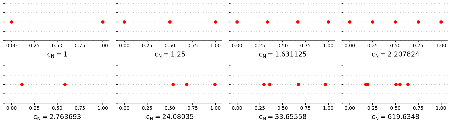
To get a better understanding of the properties of norming sets and the corresponding norming constants we graphically analyze several natural candidates. In Figure 1 we plot several possible norming sets in $d=1$ and provide the associated norming constants. First, note that as the cardinality of the norming sets increases with respect to the order of polynomials, the norming constants also increase. The reason behind is that higher order polynomial spaces $\mathscr{P}_{l}(\Omega)$ are consist of more elements and therefore it is more difficult to characterize them with a finite set of functionals. Second, one can observe that for randomly chosen points $w_{j}$, the norming constant is substantially higher than for equidistant design.
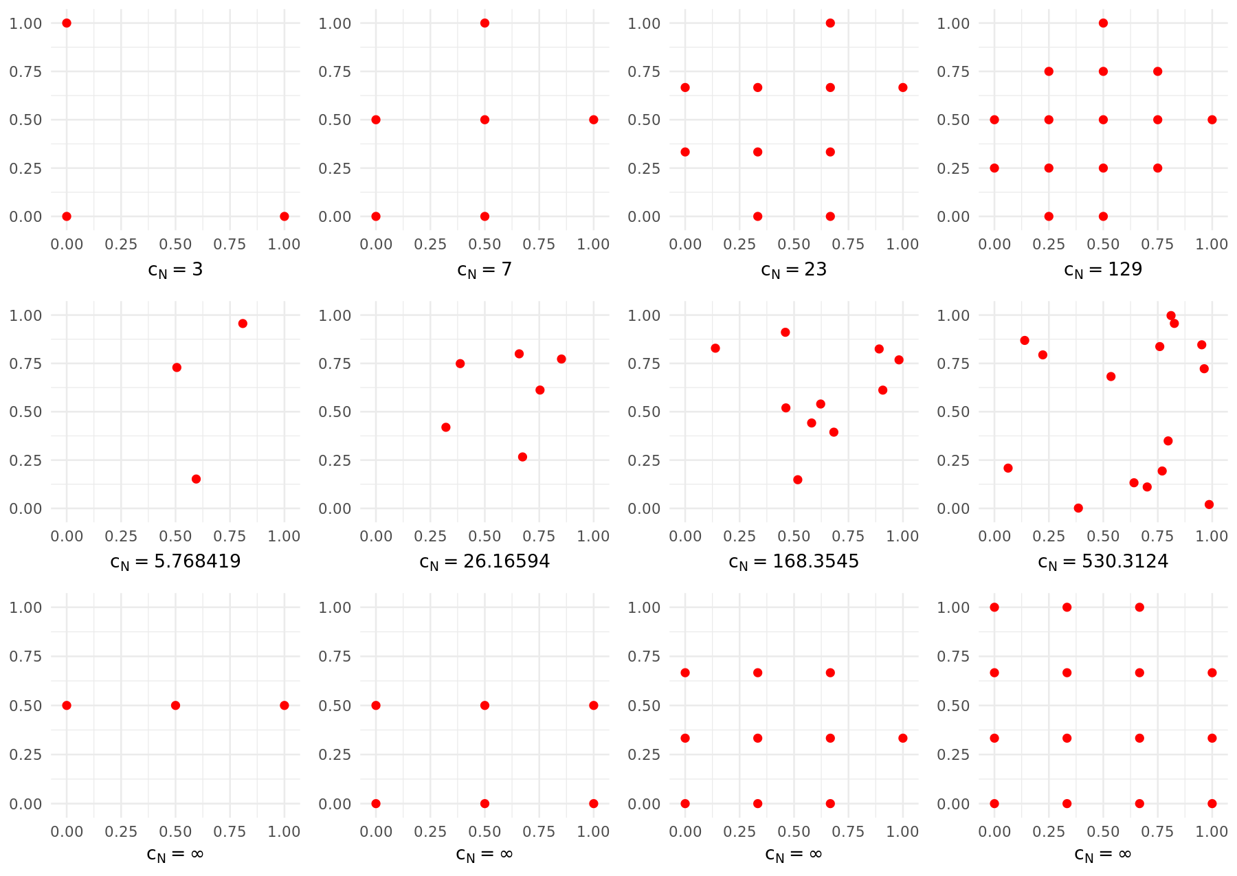
In Figure 2 we consider the $d=2$ case. Similarly to the one dimensional case one can notice the increase of the norming constants in the order of the polynomials. Furthermore, the norming constants are smaller for regular, fixed design than for i.i.d. samples generated from uniform distribution. This is especially the case for “corner sets”, a carefully designed unisolvent set capturing the local polynomial structure that will be introduced in Section 3.3.2. Moreover, for $d\geq 2$, there also exist sets with cardinality ${l+d\choose l}$ that are not norming sets for the space of polynomials up to $l$th order. We provide these examples at the bottom row of Figure 2.

Refer to caption
Figure 1: Norming sets for unidimensional space. Top row: Equally spaced points on a unidimensional grid for $1,2,3,4$th order polynomials; Bottom row: Sets consist of i.i.d. samples from uniform distribution, where each plot pictures a set with the same cardinality as the plot directly above it.
Refer to caption
Figure 2: Norming sets in 2-dimensional space. The cardinality for sets in $i$th ($1\leq i\leq 4$) row is ${i+2\choose i}$, the dimension for linear spaces spawned by polynomials up to $i$th order. Top row: “corner sets” on a two-dimensional grid for $1,2,3,4$th order polynomials; Middle row: Sets consist of i.i.d. samples from the uniform distribution; Bottom row: Artificially generated sets that are NOT norming sets for the corresponding polynomial spaces.

3.3 Layered Norming DAGs

After introducing in the previous sections the background regarding polynomials, we propose principled DAG structures to be used in the Vecchia approximation. After rigorously defining them below, we provide algorithms for obtaining them in practice.

3.3.1 The Layered and Norming Conditions

We define the Layered Norming DAGs based on the layered and the norming conditions. For simplicity, we assume the training set $\mathcal{X}_{n}=\{X_{1},X_{2},\cdots,X_{n}\}$ is a subset of $[0,1]^{d}$.

We start by describing the Layered condition on the considered DAGs.

Condition 1 (Layered).

We consider a directed acyclic graph with a partition of its vertex set $\mathcal{X}_{n}=\cup_{j=0}^{J}\mathcal{N}_{j}$ satisfying that

  • $\forall X_{i}\in\mathcal{N}_{j}$, $\mathrm{pa}(X_{i})\subset\cup_{j^{\prime}=0}^{j-1}\mathcal{N}_{j^{\prime}}$;

  • There exist constants $\gamma>1$, $c_{d}>0$, such that $\forall X_{i_{1}},X_{i_{2}}\in\cup_{j^{\prime}=0}^{j}\mathcal{N}_{j^{\prime}}$, $\|X_{i_{1}}-X_{i_{2}}\|_{\infty}\geq c_{d}\gamma^{-j}$.

In the rest of the paper, we assume indices for elements in $\mathcal{X}_{n}$ are already ordered based on their corresponding layers. That being said, let $\eta(i)$ be the layer of $X_{i}$ such that $X_{i}\in\mathcal{N}_{\eta(i)}$, then for all $X_{i},X_{i^{\prime}}\in\mathcal{X}_{n}$ with $i<i^{\prime}$, we have $\eta(i)\leq\eta(i^{\prime})$.

The layered condition, as the name suggests, partitions the training set $\mathcal{X}_{n}$ into $J+1$ layers $\mathcal{N}_{0},\mathcal{N}_{1},\ldots,\mathcal{N}_{J}$, such that for any element $X_{i}$ in layer $\mathcal{N}_{j}$, the associated parents can only come from layers preceding $\mathcal{N}_{j}$. Moreover, the minimum distance between the elements is governed by their respective layers. The overall design of the layered structure encourages the “coarse to fine” framework, where the first few layers tend to be relatively spread out in the domain while the latter layers gradually fill in the gaps of the domain. Such layered set structure can be chosen for arbitrary training set $\mathcal{X}_{n}$, see the algorithms in the next section. Next we introduce the Norming condition for DAGs.

Condition 2 (Norming).

Consider a DAG satisfying Condition 1 with parameter $\gamma>1$. Assume that for $m={\underline{\alpha}+d\choose\underline{\alpha}}$, there exists $i_{0}\in\mathbb{N}$, such that for all $i\geq i_{0}$, $|\mathrm{pa}(X_{i})|=m$. Moreover, there exist constants $c_{L},c_{N}>0$, such that for all $X_{i}\in\mathcal{N}_{j}$, with $0\leq j\leq J$ and $i\geq i_{0}$, there exists a $d$-dimensional cube $\mathcal{C}\supset\mathrm{pa}(X_{i})\cup\{X_{i}\}$ with side length no greater than $c_{L}\gamma^{-j}$, such that $\mathrm{pa}(X_{i})$ is a norming set on $\mathscr{P}_{\underline{\alpha}}(\mathcal{C})$ with norming constant $c_{N}$.

The above norming condition, built upon the layered condition, requires that the parent set of each $X_{i}$ (from a threshold $i_{0}$ onwards) is norming set on a neighborhood of $X_{i}$. Moreover, it assumes the existence of a universal norming constant $c_{N}$ for these norming sets. Unlike Condition 1 that can be satisfied for all $\mathcal{X}_{n}$ with a properly built DAG, the norming condition doesn’t hold necessarily. It can be shown that an arbitrary sample of size $m={l+d\choose l}$ with respect to a measure, which is absolutely continues with respect to Lebesgue measure, forms a unisolvent set for $l$th order polynomial interpolation, with probability one. However, the corresponding norming constant can be arbitrarily large with positive probability. In fact, some datasets are innately unable to support a DAG satisfying the norming condition, while other datasets require careful consideration when building the DAG, as will be discussed in the next subsection.

3.3.2 Building Layered Norming DAGs

In this section we focus on providing constructive algorithms for finding norming sets with small norming constants. This is a challenging problem, especially in high-dimensional spaces. More concretely, we first propose a method for building DAGs that satisfy Conditions 1 and 2 on the perturbed grid. The more technical problem of generally located data $\mathcal{X}_{n}$ is deferred to Section A.4 of the supplementary materials

For notational convenience suppose that $n=\tilde{n}^{d}$ for some $\tilde{n}\in\mathbb{N}$. The data set $\mathcal{X}_{n}$ of the form

$\displaystyle\mathcal{X}_{n}=\big{\{}(x_{i_{1},1},x_{i_{2},2},\ldots,x_{i_{d},d}):1\leq i_{1},i_{2},\cdots,i_{d}\leq\tilde{n}\big{\}}$ (17)

is called a perturbed grid if there exist constants $0<c_{1}\leq c_{2}$, such that $c_{1}\leq x_{i+1,h}-x_{i,h}\leq c_{2}$, for all $h\in\{1,...,d\}$ and $i\in\{1,...,\tilde{n}-1\}$. In other words, $\mathcal{X}_{n}$ is the tensor product of the sets $\{x_{1,h},x_{2,h},\cdots,x_{\tilde{n},h}\}$ for all $h$. The name originates from taking the tensor product of monotone increasing sequences closely resembling the unidimensional grid. For $c_{1}=c_{2}$ the set $\mathcal{X}_{n}$ exactly forms a grid.

First we construct layered norming DAGs on perturbed grid data for $\tilde{n}=2^{r}+1$, $r\in\mathbb{N}$ and then discuss the extension to general $\tilde{n}\in\mathbb{N}$. Recalling the definition of the perturbed grid in (17), we construct the $j$th layer $\mathcal{N}_{j}$ as

$$\mathcal{N}_{j}=\big{\{}(x_{i_{1},1},\ldots,x_{i_{d},d}):(i_{h}-1)\;\mathrm{mod}\;2^{r-j}=0,\;(i_{h}-1)\;\mathrm{mod}\;2^{r-j-1}\neq 0,\forall 1\leq h\leq d\big{\}}.$$ (18)

Observe that $\mathcal{N}_{j}$ satisfies Condition 1 with $\|\cdot\|$ denoting the $\ell^{\infty}$ norm, $\gamma=2$ and parameter $c_{d}\leq(c_{2}+c_{1})/(2c_{1})$. It remains to specify the parent sets $\mathrm{pa}(X_{i})$ for all $X_{i}$ such that they form norming sets. For all $j$ large enough such that $\cup_{0\leq j^{\prime}\leq j-1}\mathcal{N}_{j^{\prime}}$ has at least $l^{d}$ elements, for all $X_{i}\in\mathcal{N}_{j}$, we choose the corresponding “corner” set as parent set, see Section 3 of [40].

The corner set built around $X_{i}$ basically consists the elements of $\mathcal{X}_{n}$ which are in the $l$-radius neighbourhood of $X_{i}$ with respect to the $\ell_{1}$-metric on the grid (where the distance between neighbouring grid points is set to 1). More formally, for all $1\leq h\leq d$, let us first project the points in $\cup_{0\leq j^{\prime}\leq j-1}\mathcal{N}_{j^{\prime}}$ into their $h$th coordinate and then sort them in an increasing order with respect to their distance from $X_{i}[h]$. We denote this ordered set by $B_{h}=(x_{s(1),h},x_{s(2),h},\cdots,x_{s(n^{\prime}),h})$, where $n^{\prime}=2^{j-1}+1$ is the cardinality of projected set. The corner parent set of $X_{i}$ is defined as

$$\mathrm{pa}(X_{i})=\Big{\{}(x_{s(i_{1}),1},x_{s(i_{2}),2},\cdots,x_{s(i_{d}),d}):\sum_{h=1}^{d}[i_{h}-1]\leq l\Big{\}}.$$ (19)

First note that the cardinality of the set $\mathrm{pa}(X_{i})$ is exactly ${l+d\choose l}$. Furthermore, it is unisolvent whose interpolation polynomial can be explicitly written in multivariate divided-difference formula, see Theorem 5 of [40]. However, unlike in the unidimensional case, for $d\geq 2$, such divided-difference formula does not provide a simple, easily applicable formula with Lagrangian polynomials. At the same time, in view of Lemma 3, the norming constant is scale invariant and therefore only depends on the ratio of $c_{2},c_{1}$. Hence, for given $c_{1},c_{2}$, there exists a constant $c_{N}>0$, such that $\mathrm{pa}(X_{i})$ is a norming set with this norming constant. The computation of the explicit formula for $c_{N}$ is challenging and is outside of the scope of this paper. Nevertheless, we demonstrate in Figure 2 through simple examples the extent of the norming constant. Furthermore, we also note that the set $\mathrm{pa}(X_{i})\cup\{x\}$ is contained in a $d$-dimensional cube with diameter bounded from above by $2^{-j}(l+1)c_{2}/c_{1}$. Therefore, Condition 2 is satisfied.

Finally, for $\tilde{n}\neq 2^{r^{\prime}}+1$, $r^{\prime}\in\mathbb{N}$, let $r$ be the largest integer such that $\tilde{n}>2^{r}+1$. Then take $\mathscr{I}\subset\{1,2,\cdots,\tilde{n}\}$ with cardinality $2^{r}+1$ such that its complement doesn’t contain consecutive integers. Then we consider the subset of $\mathcal{X}_{n}$ defined by

$$\tilde{\mathcal{X}}_{n}=\big{\{}(x_{i_{1},1},x_{i_{2},2},\cdots,x_{i_{d},d}):i_{h}\in\mathscr{I},\forall 1\leq h\leq d\big{\}}.$$ (20)

Note that $\tilde{\mathcal{X}}_{n}$ forms a perturbed grid with cardinality $(2^{r}+1)^{d}$ and therefore one can build a layered norming DAG on it. Once this is done, we let the layer $\mathcal{N}_{r+1}=\mathcal{X}_{n}\backslash\tilde{\mathcal{X}}_{n}$. Then, for all $X_{i}\in\mathcal{N}_{r+1}$, we define a corner parent set, similarly as in equation (19). We formalize the above method in Algorithm 2, deferred to Section A.4 of the supplementary materials.

4 Probabilistic Properties

In this section, we study the probabilistic properties of Vecchia GPs associated to mother GPs with Matérn covariance kernels given in Section 1.3. The existing theoretical analysis of Matérn processes heavily relies on the explicit form of the covariance kernel and its Fourier transform. Unfortunately, in case of Vecchia GPs the covariance matrices of their finite dimensional marginals can only be obtained by inverting the precision matrices, rendering the direct analyzes substantially more difficult. Moreover, the covariance kernel of the Vecchia approximated Matérn process is not stationary, hence the techniques relying on the spectral density of the Matérn process can no longer be applied. This necessitates the development of new mathematical tools built on the finite dimensional conditional distributions of the GP.

We organize this section on the probabilistic properties of Vecchia GPs associated to Matérn covariance kernels as follows. In Section 4.1 we recall some properties of the Matérn Gaussian process $Z^{\tau,s}_{X}$. Section 4.2 studies the conditional distribution of $Z^{\tau,s}_{X}$ given the same process at $\mathrm{pa}(X)$. Section 4.3 utilizes the result of Section 4.2 to derive small deviation bounds for the Vecchia GP $\hat{Z}^{\tau,s}_{X}$ associated to the Matérn mother GP. Finally, Section 4.4 studies the approximation properties of Vecchia GPs, which in turn provide the de-centered small ball probabilities. Throughout the section, whenever a DAG is involved, we assume that Conditions 1 and 2 are satisfied with some positive constants $c_{d},c_{L}$ and $c_{N}$ not depending on the sample size $n$.

The proofs for the lemmas and theorems in Section 4.1 and 4.2 are provided in Section B, while proofs for the lemmas and theorems in Section 4.3 and 4.4 are deferred to Section C of the supplementary materials.

4.1 Matérn Process

We first discuss some results regarding the derivatives of Matérn covariance functions. The differentiability of Matérn covariance functions are well-known [55, 22], but the Lipschitz continuity result in equation (23) is relatively obscure, with its $\alpha\not\in\mathbb{N}$ case provided in [51] without proofs. For the sake of clarity and completeness, we state and prove all these results here.

Lemma 4.

Let $K(\cdot,\cdot)$ denote the Matérn covariance kernel with regularity parameter $\alpha>0$, see the definition in (2). Then $K(\cdot,\cdot)$ is $2\underline{\alpha}$ times differentiable on $\mathbb{R}^{2d}$, such that $\forall\;|k_{1}|+|k_{2}|\leq 2\underline{\alpha}$ and $\forall\;x_{1},x_{2}\in\mathbb{R}^{d}$,

$$|K^{(k_{1},k_{2})}(x_{1},x_{2})|\lesssim 1.$$ (21)

Furthermore, for all $|k|\leq\underline{\alpha}$, $K^{(k,k)}(x_{1},x_{2})$, we have

$$K^{(k,k)}(x_{1},x_{2})=K^{(k,k)}(x_{2},x_{1}),\;\;K^{(k,k)}(x_{1},x_{1})=K^{(k,k)}(x_{2},x_{2}).$$ (22)

Finally, for all $|k_{1}|+|k_{2}|=2\underline{\alpha}$, $x\in\mathbb{R}^{d}$ and $h\in\mathbb{R}^{d}$ small enough, we have

$$|K^{(k_{1},k_{2})}(x,x)-K^{(k_{1},k_{2})}(x,x+h)|\lesssim\bigg{\{}\begin{aligned} &\|h\|_{2}^{2(\alpha-\underline{\alpha})},\;\;&&\alpha\not\in\mathbb{N},\\ &\|h\|^{2}_{2}\ln(1/\|h\|_{2}),\;\;&&\alpha\in\mathbb{N}.\end{aligned}$$ (23)

Lemma 4 shows the the Matérn covariance function $K(\cdot,\cdot)$, viewed as a function from $\mathbb{R}^{2d}\to\mathbb{R}$, is $2\underline{\alpha}$ times differentiable, with Lipschitz continuous $2\underline{\alpha}$th order derivatives. Matérn covariance function belong to $C^{\alpha}(\mathbb{R}^{d})\times C^{\alpha}(\mathbb{R}^{d})$ in the sense that for integer $\alpha$ the function is weakly differentiable of the order $(k,k),\forall|k|=\alpha$. However, the Hölder-$(\alpha,\alpha)$ norm is infinite since the weak derivatives of the order $(k,k),\forall|k|=\alpha$ are not uniformly bounded. Moreover, the sample paths of the process are almost surely $\underline{\alpha}$ times differentiable with their $\underline{\alpha}$th derivatives being almost surely Lipschitz continuous of order $\alpha-\underline{\alpha}$, up to a logarithm term.

The smoothness properties described in Lemma 4 carry over to the covariance kernels of the conditional processes as well. More precisely, for an arbitrary finite set $A=\{w_{1},w_{2},\cdots,w_{m}\}\subset\mathbb{R}^{d}$, let us define the process $\tilde{Z}$ as

$$\tilde{Z}_{x}=Z_{x}-\mathbb{E}(Z_{x}|Z_{A})=Z_{x}-K_{x,A}K_{A,A}^{-1}Z_{A}.$$

By the linearity of the operator one can observe that $\tilde{Z}$ is also a centered GP with covariance function

$$\tilde{K}(x_{1},x_{2})=\mathbb{E}\tilde{Z}_{x_{1}}\tilde{Z}_{x_{2}}=K(x_{1},x_{2})-K_{x_{1},A}K_{A,A}^{-1}K_{A,x_{2}}.$$ (24)

The process $\tilde{Z}$ can be regarded as the “conditional” Gaussian process on the set $A$. We show below that it inherits many properties of the mother Matérn process $Z$. Remarkably, these properties do not depend on the conditioning set $A$.

Lemma 5.

Let $\tilde{K}(\cdot,\cdot)$ be the covariance function defined in (24). Then $\tilde{K}(\cdot,\cdot)$ is $2\underline{\alpha}$ times differentiable on $\mathbb{R}^{2d}$ and for all $|k|\leq\underline{\alpha}$,

$$|\tilde{K}^{(k,k)}(x_{1},x_{2})|\lesssim 1.$$ (25)

Moreover, for all $|k|=\underline{\alpha}$, $x\in\mathbb{R}^{d}$ and $h\in\mathbb{R}^{d}$ small enough, we have

$\displaystyle\big{|}\tilde{K}^{(k,k)}(x,x)-\tilde{K}^{(k,k)}(x,x+h)-\tilde{K}^{(k,k)}(x+h,x)+\tilde{K}^{(k,k)}(x+h,x+h)\big{|}$
$\displaystyle\qquad\quad\lesssim\bigg{\{}\begin{aligned} &\|h\|_{2}^{2(\alpha-\underline{\alpha})},\;\;&&\alpha\not\in\mathbb{N},\\ &\|h\|_{2}^{2}\ln(1/\|h\|_{2}),\;\;&&\alpha\in\mathbb{N}.\end{aligned}$ (26)

All constant multipliers in the upper bounds are independent of $x,h\in\mathbb{R}^{d}$ and the set $A$.

The intuition behind the universality of the constants in Lemma 5 across the different conditional sets $A$ is that the “variance” of the conditional process $\tilde{Z}$ can not exceed the variance of its mother GP’s $Z$. In view of the relationship between derivatives of Gaussian processes and the derivative of the covariance functions established in Proposition I.3 of [22], the above intuition applies not only to the processes $Z$ and $\tilde{Z}$, but also to their derivative processes, up to order $\underline{\alpha}$. As a result, regardless to the conditioning set $A$, the conditional process $\tilde{Z}$ inherits similar smoothness properties as the mother Gaussian process $Z$. This feature plays a crucial role in the development of conditional distributions in the next sections. We also note that the logarithmic term in the previous lemmas for $\alpha\in\mathbb{N}$ follows from the singularity of the modified Bessel functions of second kind at integer parameters. In the rest of the paper, for simplicity of notations, we use $[\ln(1/\|h\|_{2})]^{\mathbbm{1}_{\{\alpha\in\mathbb{N}\}}}$ to denote that the logarithm only occurs for integer $\alpha$ values.

4.2 Conditional Distribution

The conditional distribution formulas (7) and (2.2) defining the Vecchia GPs are the starting point of our theoretical analysis. In this section, we study three aspects of these conditional distributions: the variance in equation (2.2), the conditional expectation in equation (2.2), and the effect of recursively applying this conditional expectation formula.

4.2.1 Variance and Conditional Expectation

Under the Norming Condition 2, the distance among elements in the set $\mathrm{pa}(X_{i})\cup\{X_{i}\}$ is bounded by $\gamma^{-\eta(i)}$ up to a constant multiplier, where $\eta(i)=j$ denotes the layer allocation of $X_{i}\in\mathcal{N}_{j}$. We recall, that the observations are ordered based on their layer allocations, hence the functions $i\rightarrow\eta(i)$ is monotone increasing. We investigate the asymptotic behavior of the Gaussian random variable $Z^{\tau,s}_{X_{i}}-\mathbb{E}[{Z}^{\tau,s}_{X_{i}}|{Z}^{\tau,s}_{\mathrm{pa}(X_{i})}]$ as $i$ goes to infinity. The following theorem provides lower and upper bounds for its variance, which coincides with the variance of the conditional Matérn GP process.

Theorem 1.

Let the mother Gaussian process $Z^{\tau,s}$ be the rescaled Matérn process with smoothness parameter $\alpha$. Suppose Condition 2 is satisfied, then for all $X_{i}\in\mathcal{N}_{j}$, $j=1,...,J$, we have

$\displaystyle\mathrm{Var}\big{\{}Z^{\tau,s}_{X_{i}}-\mathbb{E}[{Z}^{\tau,s}_{X_{i}}|{Z}^{\tau,s}_{\mathrm{pa}(X_{i})}]\big{\}}\asymp s^{2}\tau^{2\alpha}\gamma^{-2\alpha j}(\ln\gamma)^{\mathbbm{1}_{\{\alpha\in\mathbb{N}\}}}.$ (27)

Theorem 1 is essential in determining the small ball probabilities of Vecchia GPs. Specifically, for a finite training set $\mathcal{X}_{n}$, the number of layers $\eta(n)$ satisfies $\gamma^{d\eta(n)}\asymp n$. Therefore, for $X_{i}\in\mathcal{N}_{\eta(n)}$, ignoring the rescaling parameters $\tau,s$, we have $\mathrm{Var}\big{\{}Z_{X_{i}}-\mathbb{E}[{Z}_{X_{i}}|{Z}_{\mathrm{pa}(X_{i})}]\big{\}}\asymp n^{-2\alpha/d}.$ In other words, the variance of $X_{i}\in\mathcal{N}_{\eta(n)}$ goes to zero with a polynomial rate in $n$, where the order is proportional to the smoothness parameter $\alpha$ of the mother Matérn process. Hence smoother mother GPs posses faster decaying variances (27).

We proceed to study the conditional expectation $\mathbb{E}[\hat{Z}^{\tau,s}_{X_{i}}|\hat{Z}^{\tau,s}_{\mathrm{pa}(X_{i})}]$ in equation (2.2), which is a Gaussian interpolation333Also called kriging in spatial statistics literature[19]. of $\hat{Z}^{\tau,s}_{X_{i}}$ using the random vector $\hat{Z}^{\tau,s}_{\mathrm{pa}(X_{i})}$. Before discussing its properties, we first introduce some notations. Let $x^{*}\in\mathcal{X}$ be a singleton in $\mathcal{X}$ and $A=\{w_{i},1\leq i\leq m\}\subset\mathbb{\mathcal{X}}$ be a fixed set. For scaler $\tau>0$, the set $\tau A$ consists of the elements of $A$ multiplied by $\tau$. Then the objective is to study the coefficients of the following conditional expectation

$$\mathbb{E}(Z^{\tau,s}_{x^{*}}|Z^{\tau,s}_{A})=K_{\tau A,\tau x^{*}}^{T}K_{\tau A,\tau A}^{-1}Z^{\tau,s}_{A},$$ (28)

where $\tau$ might tend to zero. Note that the conditional expectation in (28) highly depends on the covariance function $K$, characterizing the spatial dependencies of the process $Z$. However, we show below, that under certain regularity conditions, for fixed $x^{*}$ and $A$ and letting $\tau$ go to zero, the limit for $K_{\tau A,\tau A}^{-1}K_{\tau A,\tau x^{*}}$ is free of the covariance function. This limit is often referred to as the “flat limit” in the literature of radial basis functions [15, 46, 36]. For Matérn covariance functions, the following lemma shows that the flat limit coincides with the polynomial interpolation coefficients if the set $A$ is a norming set with respect to an appropriately chosen families of polynomials.

Lemma 6.

Let $A$ be a norming set on $\mathscr{P}_{l}([0,1]^{d})$ with $l\leq\underline{\alpha}$ and norming constant $c_{N}$. Suppose $x\in[0,1]^{d}$, then we have for all $\tau<1$,

$$\big{\|}K_{\tau A,\tau A}^{-1}K_{\tau A,\tau x}-V_{A}^{-1}v_{x}\big{\|}_{1}\lesssim\tau^{2(\alpha-\underline{\alpha})}[\ln(1/\tau)]^{\mathbbm{1}_{\{\alpha\in\mathbb{N}\}}}+\tau.$$ (29)

Similarly, for $\tau_{0}\in(0,+\infty)$ and $\tau\in(0,+\infty)\cap(\tau_{0}-1,\tau_{0}+1)$, we have

$$\big{\|}K_{\tau A,\tau A}^{-1}K_{\tau A,\tau x}-K_{\tau_{0}A,\tau_{0}A}^{-1}K_{\tau_{0}A,\tau_{0}x}\big{\|}_{1}\lesssim|\tau-\tau_{0}|^{2(\alpha-\underline{\alpha})}[\ln(1/|\tau-\tau_{0}|)]^{\mathbbm{1}_{\{\alpha\in\mathbb{N}\}}}+|\tau-\tau_{0}|.$$ (30)

All the constants in $\lesssim$ are independent of $x$ and $A$.

Lemma 6 provides an example of flat limits of radial basis function interpolation, a topic with extended literature, studied over twenty years, see for instance [15, 36]. The general idea is that for smooth enough kernels (i.e. Matérn covariance functions in our case) and unisolvent set $A$ with respect to some families of polynomials, the limit of equation (28) becomes the interpolation within that polynomial family. With this in mind, we discuss the conditions of Lemma 6. The requirement “smooth enough” is relative to the set $A$. For the set $A$ to be a norming set of a polynomial space, a necessary condition is that the cardinality of $A$ must be no smaller than the dimension of this polynomial space. The covariance function $K(\cdot,\cdot)$ of the Matérn process with regularity $\alpha$ belongs to $C^{2\underline{\alpha}}$, i.e., it is $\underline{\alpha}$ times differentiable in both variables. Therefore, the polynomial spaces that describe the local behavior of Matérn covariance function is the space $\mathscr{P}_{\underline{\alpha}}([0,1]^{d})$, which has dimension ${\underline{\alpha}+d\choose\underline{\alpha}}$. Letting ${\underline{\alpha}+d\choose\underline{\alpha}}\geq{l+d\choose l}$, we get the condition that $l\leq\underline{\alpha}$.

Next we discuss the issue of choosing a norming set $A$ with uniformly bounded norming constant $c_{N}$. Recall, that $A$ is a norming set if it is a unisolvent set with respect to some polynomials. In the unidimensional case, a set $A$ with $m$ distinct elements is always unisolvent with respect to the polynomials up to $(m-1)$th order. In higher dimensions $d\geq 2$, however, it is possible that the elements of $A$ belong to a lower dimensional polynomial manifold and, as a consequence, the corresponding Vandermonde matrix $V_{A}$ is singular. In such cases, the limit of Gaussian interpolation on the set $A$ is interpreted within a family of lower order polynomials. We note that the assumption of $A$ being exactly a unisolvent set of $\mathscr{P}_{l}([0,1]^{d})$ is not necessary. The limit of equation (28) still exists when choosing arbitrary ${l+d\choose l}\leq m<{l+1+d\choose l+1}$. However, the corresponding formulas are more complex, depending on the derivatives of covariance function at the origin, see [36]. It is also worth noting that in case the set $A$ is a strict superset of a norming set for $\mathscr{P}_{l}([0,1]^{d})$, then although the limit of equation (28) exists, it is very unlikely to be polynomial interpolation. For instance in case $\alpha$ is an even integer the limit is the polyharmonic spline interpolation, see [46]. We are not aware of any literature that addresses this limit in a more general setting. Therefore, for simplicity, we consider unisolvent sets from now on. Finally, the norming constant $c_{N}$ appears in the upper bound (29). Therefore, $c_{N}$ has to be universal, not depending on the sample size $n$, otherwise it would interfere the rate in equation (29).

Finally, we would like to mention that our Lemma 6 extends the results of [36] by providing the explicit convergence rate of the Gaussian interpolation to the polynomial interpolation. Moreover, these rates are uniform in $x\in\mathbb{R}^{d}$ if $A$ is unisolvent with a universal norming constant $c_{N}$. Such explicit bounds are required for the small deviation bounds of the GP.

4.2.2 Recursive Interpolation

Another important issue regarding Vecchia Gaussian processes arises from repeatedly applying the conditional expectation formula. Specifically, for all $X_{i}\in\mathcal{X}$, we denote the “double parent” set of $X_{i}$ as $\mathrm{pa}^{2}(X_{i})\triangleq\cup_{X\in\mathrm{pa}(X_{i})}\mathrm{pa}(X)$. Despite the conditional distribution of $X_{i}$ given its parent set $\mathrm{pa}(X_{i})$ is the same for the process $Z^{\tau,s}$ and its Vecchia approximation $\hat{Z}^{\tau,s}$, the conditional distribution of $X_{i}$ given its double parent set $\mathrm{pa}^{2}(X_{i})$ is often different in these two processes. In other words, applying the conditional expectation formula of Vecchia Gaussian processes more than once will result in different conditional distributions from the mother GP.

Therefore, to formally study the properties of Gaussian interpolation we introduce the corresponding operator $G_{j}$ that maps a function $f:\cup_{j^{\prime}=0}^{j}\mathcal{N}_{j^{\prime}}\to\mathbb{R}$ to a function $G_{j}(f):\cup_{j^{\prime}=0}^{j+1}\mathcal{N}_{j^{\prime}}\to\mathbb{R}$. Specifically,

$$G_{j}(f)(X)=\Bigg{\{}\begin{aligned} &f(X),&&\forall X\in\cup_{j^{\prime}=0}^{j}\mathcal{N}_{j^{\prime}},\\ &K_{\tau\mathrm{pa}(X),\tau X}^{T}K_{\tau\mathrm{pa}(X),\tau\mathrm{pa}(X)}^{-1}\bm{f}({\mathrm{pa}(X)}),&&\forall X\in\mathcal{N}_{j+1}.\end{aligned}$$ (31)

In view of Lemma 6, the limit of the Gaussian interpolation is the polynomial interpolation. Let us denote the polynomial interpolation operator $P_{j}$ mapping a function $f:\cup_{j^{\prime}=0}^{j}\mathcal{N}_{j^{\prime}}\to\mathbb{R}$ to a function $P_{j}(f):\cup_{j^{\prime}=0}^{j+1}\mathcal{N}_{j^{\prime}}\to\mathbb{R}$ as

$$P_{j}(f)(X)=\Bigg{\{}\begin{aligned} &f(X),&&\forall X\in\cup_{j^{\prime}=0}^{j}\mathcal{N}_{j^{\prime}},\\ &v_{\tau X}^{T}V_{\tau\mathrm{pa}(X)}^{-T}\bm{f}({\mathrm{pa}(X)})=v_{X}^{T}V_{\mathrm{pa}(X)}^{-T}\bm{f}({\mathrm{pa}(X)}),&&\forall X\in\mathcal{N}_{j+1}.\end{aligned}$$

Furthermore, let us endow the space of functions on $\cup_{j^{\prime}=1}^{j}\mathcal{N}_{j^{\prime}}$ with the supremum norm $\ell^{\infty}$. Then in view of Lemma 6, the difference between the operators $G_{j}$ and $P_{j}$ tend to zero in operator norm. Therefore, it is sufficient to study the recursive interpolation with the polynomial operators $P_{j},j\in\mathbb{N}$. In fact, we aim to show that the following assertion holds, formulated as a condition below.

Condition 3.

Let $P_{j},j\geq 0$ be the polynomial interpolation operator defined on the DAG of the Vecchia Gaussian process $\hat{Z}^{\tau,s}$. Then for all $0\leq j_{1}\leq j_{2}\leq\eta(n)$, $\forall f\in\ell^{\infty}(\cup_{j^{\prime}=0}^{j_{1}}\mathcal{N}_{j^{\prime}})$,

$$\|P_{j_{2}}P_{j_{2}-1}\cdots P_{j_{1}}(f)\|_{\infty}\lesssim\|f\|_{\infty},$$ (32)

where the constant in “$\lesssim$” is independent of $j_{1}$ and $j_{2}$.

Condition 3 is determined by the data set $\mathcal{X}_{n}$ and the DAG built on the top of it. It plays a crucial role in our proof for the posterior contraction rates of the Vecchia GP, when controlling the size of the recursive GP interpolation. Despite the numerous numerical evidence, this condition is extremely challenging to prove for general data sets $\mathcal{X}_{n}$. Therefore, we restrict ourselves to perturbed grid data. We use data argumentation to eliminate border effects, which allows us to view polynomial interpolations as convolution operators and study their Fourier transforms. We defer the technical details to the supplementary materials and only state the conclusions here.

Lemma 7.

Suppose Condition 2 holds, $\mathcal{X}_{n}$ is a perturbed grid data and the DAG of the Vecchia GP is defined by Algorithm 3 in the supplementary materials. If one of the following statements holds:

  • $d=1$ and $\underline{\alpha}$ is an even integer or $\underline{\alpha}\leq 100$,

  • $d=2$ and $\underline{\alpha}\leq 16$,

then Condition 3 holds.

We comment on the conditions of Lemma 7. Although the combinations of $d,\alpha$ may look restrictive at first glance, they in fact cover the cases typically considered in geostatistical applications. In such applications, the domain is a geological space with dimension $d$ equals $1$ or $2$ and the regularity parameter $\alpha$ typically does not exceed $5/2$. Moreover, our proof techniques can be extended beyond these values of $d$ and $\alpha$. The bottle neck is the design of an operator on Fourier space and the numerical evaluation of an equation involving close-to-singular quantities of this operator. The technical and cumbersome nature of such extension is beyond the scope of this paper.

Remark 1.

As mentioned earlier, it is very challenging to verify Condition 3 for general data set $\mathcal{X}_{n}$. While the operator norm for each individual operator $P_{j},j\in\mathbb{N}$ can be controlled, such results do not imply the condition. Specifically, in the considered DAGs of Vecchia GPs, the total number layers is $\eta(n)\asymp\ln n$. Therefore, even if we have a uniform control over the operators $\|P_{j}\|\leq c,\forall j\in\mathbb{N}$ for some constant $c>1$, the repeated interpolation can still blow up

$$\|P_{J-1}P_{J-2}\cdots P_{1}P_{0}\|\leq n^{\ln c},\qquad\text{with $J=\ln n$}$$

Therefore, we need to consider the composition of these operators as a whole, which is exceedingly difficult to handle without structural or geometrical assumptions on $\mathcal{X}_{n}$. The case becomes considerably easier for close to grid data, since here the polynomial interpolation is equivalent to convolution, which can be further converted to multiplication via Fourier transform. In Lemma 7, we use semi-explicit computations for the composition of the operators $P_{j},j\in\mathbb{N}$.

Then, by combining Lemma 6 and Condition 3, we can conclude that the operator norms of the recursive Gaussian interpolations are bounded.

Lemma 8.

Under Conditions 2 and 3, we have for all $0\leq j_{1}\leq j_{2}$,

$$\|G_{j_{2}}\cdots G_{j_{1}+1}G_{j_{1}}\|\lesssim 1.$$

We conclude this section with some general remarks. Theorem 1 and Lemma 6 study the variance and conditional expectations that define the Vecchia GPs, while Lemma 8 shows that recursively applying Gaussian processes interpolation has bounded operator norm. These three lemmas are the building blocks for deriving the small deviation bounds for GPs, controlling the metric entropy of the associated RKHS and finally, deriving posterior contraction rates for Vecchia GPs.

4.3 Small Ball Probability

In this section, we study the small ball probability of the Vecchia Gaussian process on $\mathcal{X}_{n}$ defined as

$$\mathrm{Pr}(\|\hat{Z}^{\tau,s}_{\mathcal{X}_{n}}\|_{\infty}<\epsilon),\;\;\forall\epsilon>0.$$

Small ball probability plays a vital role in Gaussian process theories. It is directly linked to the $\epsilon$-entropy of the RKHSs (Lemma I.29 and I.30 of [22]), provides lower limits for empirical processes (Section 7.3 of [38]) and plays a crucial role in the convergence rate of the posterior [52, 51]. For Brownian motion, the small ball probability can also be interpreted as the first exit time. For more details and applications, see for instance the survey [39] and the references therein. The following lemma provides a lower bound for small ball probability or equivalently an upper bound for the small ball exponent $-\ln\mathrm{Pr}(\|\hat{Z}^{\tau,s}_{\mathcal{X}_{n}}\|_{\infty}<\epsilon)$ of the Vecchia GPs.

Theorem 2 (Small deviation bound).

Under Conditions 1, 2 and 3, if the mother Gaussian process is Matérn with smoothness parameter $\alpha$, then for $\epsilon>0$ small enough,

$$-\ln\mathrm{Pr}(\|\hat{Z}^{\tau,s}_{\mathcal{X}_{n}}\|_{\infty}<\epsilon)\lesssim\tau^{d}s^{d/\alpha}\epsilon^{-d/\alpha}[\ln(1/\epsilon)]^{\mathbbm{1}_{\{\alpha\in\mathbb{N}\}}},$$

where the constant in $\lesssim$ only depends on $\alpha$ and $\gamma_{0}$.

The proof of Theorem 2 follows a different route from the standard techniques applied for stationary Gaussian processes. Instead of deriving the small ball probability via $\epsilon$-entropy, we directly study it by utilizing the conditional distribution results derived in the previous section. The techniques are inspired by [34] and generalized in our proof. We believe these techniques are of independent interest and may be employed to analyze a broader class of stochastic processes.

For scaling parameters $\tau=s=1$, the lower bound for the small probability in Theorem 2 coincides with the Matérn process, see Lemma 11.36 of [22]. This indicates that despite having different covariance structures and lacking stationarity, the Vecchia approximation of a Matérn process has similar small deviation properties as the mother process. Such property is crucial in deriving matching posterior contraction rates for the two processes.

4.4 Decentered small ball probability

In this section we extend the above small deviations computations to the decentered case, i.e. we provide lower bounds for

$$\mathrm{Pr}(\|\hat{Z}^{\tau,s}_{\mathcal{X}_{n}}-f_{0}\|_{\infty,n}<\epsilon),\;\;\forall\epsilon>0,$$

for $f_{0}\in L_{\infty}(\Omega)$. For the analyzis we recall the definition of the RKHS associated to the Vecchia GP and discuss how its approximation properties relate to the decentered small ball probabilities.

Let us recall that the RKHS of $\hat{Z}^{\tau,s}_{\mathcal{X}_{n}}$ is

$$\mathbb{H}_{n}^{\tau,s}=\Big{\{}\sum_{i=1}^{n}a_{i}\hat{K}^{\tau,s}(X_{i},\cdot):X_{i}\in\mathcal{X}_{n},a_{i}\in\mathbb{R}\Big{\}}.$$

For all $f=\sum_{i=1}^{n}a_{i}\hat{K}^{\tau,s}(X_{i},\cdot)\in\mathbb{H}_{n}^{\tau,s}$, denote $a=(a_{1},a_{2},\cdots,a_{n})^{T}$, then its RKHS norm of the process $\hat{Z}^{\tau,s}$ can be computed as

$$\|f\|_{\mathbb{H}_{n}^{\tau,s}}^{2}=a^{T}\hat{K}^{\tau,s}_{\mathcal{X}_{n},\mathcal{X}_{n}}a.$$ (33)

For a set $A=\{x_{1},x_{2},\cdots,x_{|A|}\}$ and function $f:\mathcal{X}\to\mathbb{R}$, let us denote the vector version of $f$ as $\bm{f}(A)=(f(x_{1}),f(x_{2}),\cdots,f(x_{|A|}))^{T}.$ Then by the definition of $f$, we have

$$\bm{f}(\mathcal{X}_{n})=\hat{K}^{\tau,s}_{\mathcal{X}_{n},\mathcal{X}_{n}}a.$$ (34)

By combining equations (33), (34), we have

$\displaystyle\|f\|_{\mathbb{H}_{n}^{\tau,s}}^{2}=$ $\displaystyle\bm{f}(\mathcal{X}_{n})^{T}(\hat{K}^{\tau,s}_{\mathcal{X}_{n},\mathcal{X}_{n}})^{-1}\bm{f}(\mathcal{X}_{n}).$ (35)

We can now define the decentering function with argument $\epsilon>0$ as:

$$\inf_{f\in\mathbb{H}_{n}^{\tau,s}:\|f-f_{0}\|_{\infty,n}\leq\epsilon}\|f\|_{\mathbb{H}_{n}^{\tau,s}}^{2}.$$

The combination of the decentering function and the centered small ball exponent results in the so called concentration function

$$\phi_{f_{0},n}^{\tau,s}(\epsilon)=\inf_{f\in\mathbb{H}_{n}^{\tau,s}:\|f-f_{0}\|_{\infty,n}\leq\epsilon}\|f\|_{\mathbb{H}_{n}^{\tau,s}}^{2}-\ln\mathrm{Pr}(\|\hat{Z}^{\tau,s}_{\mathcal{X}_{n}}\|_{\infty}<\epsilon).$$ (36)

Finally, in view of Proposition 11.19 of [22], for any $f_{0}$ in the closure of the RKHS with respect to the empirical supremum norm $\|\cdot\|_{\infty,n}$, the decentered small ball probability satisfies that

$\displaystyle\phi_{f_{0},n}^{\tau,s}(\epsilon)\leq-\ln\mathrm{Pr}(\|\hat{Z}^{\tau,s}_{\mathcal{X}_{n}}-f_{0}\|_{\infty,n}<\epsilon)\leq\phi_{f_{0},n}^{\tau,s}(\epsilon/2).$ (37)

Therefore, understanding the asymptotic behaviour of the decentering function (as $\epsilon$ tends to zero with $n$) will provide us the decentered small ball probabilites.

To derive bounds for the decentering function we first provide some technical lemmas which are of interest on their own right. The first lemma discusses the minimal RKHS norm among all functions that pass some given points.

Lemma 9.

Let $Z$ be a Gaussian process defined on $\mathcal{X}$ and let $\mathbb{H}$ be its RKHS. Then for all finite sets $A=\{x_{1},x_{2},\cdots,x_{|A|}\}$ functions $f_{0}:\mathcal{X}\to\mathbb{R}$, we have

$$\inf_{f\in\mathbb{H},\bm{f}(A)=\bm{f}_{0}(A)}\|f\|_{\mathbb{H}}^{2}=\bm{f}_{0}(A)^{T}K_{A,A}^{-1}\bm{f}_{0}(A).$$

Moreover, the minimum in the above equation is obtained by the function $\sum_{i=1}^{|A|}a_{i}K(x_{i},\cdot)$, with coefficients $a=(a_{1},a_{2},\cdots,a_{|A|})^{T}=K_{A,A}^{-1}\bm{f}_{0}(A)$.

The next lemma quantifies the error of Gaussian process interpolation.

Lemma 10 (Theorem 11.4 of [54]).

For all $f\in\mathbb{H}^{\tau,s}$, we have

$$\Big{|}f(X_{i})-\mathbb{E}[Z^{\tau,s}_{X_{i}}|Z^{\tau,s}_{\mathrm{pa}(X_{i})}=\bm{f}(\mathrm{pa}(X_{i}))]\Big{|}\lesssim\sqrt{\mathrm{Var}\big{\{}Z^{\tau,s}_{X_{i}}-\mathbb{E}[{Z}^{\tau,s}_{X_{i}}|{Z}^{\tau,s}_{\mathrm{pa}(X_{i})}]\big{\}}\|f\|_{\mathbb{H}^{\tau,s}}^{2}}.$$

Finally, the following lemma quantifies the approximation error of Hölder smooth functions with the RKHS of $\hat{Z}^{\tau,s}$.

Lemma 11.

Let $f_{0}$ belong to $C^{\beta}_{1}$ with $\beta\leq\alpha$ and let $Z^{\tau,s}$ be the rescaled Matérn process with smoothness parameter $\alpha$. Under Conditions 1 and 2, for all $X_{i}\in\mathcal{X}_{n}$ and its parent set $\mathrm{pa}(X_{i})$, we have

$$\left|f_{0}(X_{i})-\mathbb{E}[Z^{\tau,s}_{X_{i}}|Z^{\tau,s}_{\mathrm{pa}(X_{i})}=\bm{f}_{0}(\mathrm{pa}(X_{i}))]\right|\lesssim\big{[}\tau^{\alpha}\gamma^{-\eta(i)\alpha}+\gamma^{-\eta(i)\beta}\big{]}(\ln\gamma)^{\mathbbm{1}_{\{\alpha\in\mathbb{N}\}}}.$$

Building on the above technical results, we can provide the following upper bound for the decentering function.

Lemma 12 (Decentering).

Let $f_{0}\in C^{\beta}_{1}$ with $\beta\leq\alpha$ and let $\hat{Z}^{\tau,s}$ be the Vecchia approximation of the rescaled Matérn process with smoothness parameter $\alpha$. Under Conditions 1 - 3, we have

$\displaystyle\inf_{f\in\mathbb{H}_{n}^{\tau,s}:\|f-f_{0}\|_{\infty,n}\leq\epsilon_{n}}\|f\|_{\mathbb{H}_{n}^{\tau,s}}^{2}\lesssim$ $\displaystyle s^{-2}\Big{[}\tau^{d}\epsilon_{n}^{-d/\alpha}+\tau^{-2\alpha}\epsilon_{n}^{-\frac{2(\alpha-\beta)+d}{\beta}}+\epsilon_{n}^{-\frac{d}{\beta}}\Big{]}[\ln(1/\epsilon_{n})]^{\mathbbm{1}_{\{\alpha\in\mathbb{N}\}}}.$

Finally, by combining the upper bounds derived for the small deviation bound and decentering function of the Vecchia GP in Theorem 2 and Lemma 12, respectively, results in an upper bound for the concentration function (36). This in turn, following from (37), provides a lower bound for the decentered small ball probability.

Lemma 13.

Let $f_{0}\in C^{\beta}_{1}$ with $\beta\leq\alpha$ and let $\hat{Z}^{\tau,s}$ be the Vecchia approximation of the rescaled Matérn process with smoothness parameter $\alpha$. Under Conditions 1 - 3, we have

$\displaystyle-\ln\mathrm{Pr}(\|\hat{Z}^{\tau,s}_{\mathcal{X}_{n}}-f_{0}\|_{\infty,n}<\epsilon)\lesssim$ $\displaystyle s^{-2}\Big{[}\tau^{d}\epsilon^{-d/\alpha}+\tau^{-2\alpha}\epsilon^{-\frac{2(\alpha-\beta)+d}{\beta}}+\epsilon^{-\frac{d}{\beta}}\Big{]}[\ln(1/\epsilon)]^{\mathbbm{1}_{\{\alpha\in\mathbb{N}\}}}$
$\displaystyle\qquad\qquad+\tau^{d}s^{d/\alpha}\epsilon^{-d/\alpha}[\ln(1/\epsilon)]^{\mathbbm{1}_{\{\alpha\in\mathbb{N}\}}}.$

5 Bayesian Nonparametrics

In this section, we provide posterior contraction rate guarantees for the Vecchia GP in context of the nonparametric regression model. With the help of the probabilistic properties developed in the previous sections, we present two main theoretical results. First we derive contraction rates of the Vecchia GP $\hat{Z}^{\tau,s}$ for fixed scaling hyper-paramateres $\tau$ and $s$ and show that optimal, oracle choices of these parameters lead to minimax optimal rates. In the second part of the section we consider the hierarchical Bayes framework with a hyper prior on the scaling parameter $(\tau,s)$. We show that this fully Bayesian approach can adapt to the minimax rate without using any knowledge of the underlying true function. The proofs for Theorem 3 and 4 and Corollary 1 and 2 are provided in Section D of supplementary materials.

5.1 Posterior Contraction Rates

There is a rich literature of posterior contraction rates for Gaussian processes that centers around the concentration function $\phi_{f_{0},n}^{\tau,s}(\epsilon_{n})$, defined in (36). In fact, the contraction rates $\epsilon_{n}$ can be obtained as the solution of the concentration inequality $\phi_{f_{0},n}^{\tau,s}(\epsilon_{n})\lesssim n\epsilon_{n}^{2}$. This is formalized in the lemma below.

Lemma 14 (Theorem 2.1 of [21]).

If there exists a sequence $\epsilon_{n}\to 0$, such that for all $f_{0}\in C^{\beta}_{1}$, the concentration function satisfies $\phi_{f_{0},n}^{\tau,s}(\epsilon_{n})\lesssim n\epsilon_{n}^{2}$, then there exists a constant $M$, such that the posterior on the regression function $f$ satisfies

$$\Pi(\|f-f_{0}\|_{\infty,n}>M\epsilon_{n}|\mathcal{D}_{n})\stackrel{{\scriptstyle P_{f_{0}}}}{{\to}}0.$$

In the previous section we have derived lower bounds for the decentered small ball probability in Lemma 13 using the upper bound on the concentration function obtained by combining Theorem 2 and Lemma 12. Therefore, by plugging in this upper bound into the concentration inequality, one can obtain the contraction rate of the posterior in view of Lemma 14.

Theorem 3.

Let $f_{0}\in C^{\beta}_{1}$, with $\beta\leq\alpha$, and $\hat{Z}^{\tau,s}$ be the the Vecchia approximation of the rescaled Matérn process with smoothness parameter $\alpha$. Under Conditions 1 - 3, we have $\Pi(\|f-f_{0}\|_{\infty,n}>M\epsilon_{n}|\mathcal{D}_{n})\stackrel{{\scriptstyle P_{f_{0}}}}{{\to}}0$ for some constant $M$ and

$$\epsilon_{n}=\max\left\{n^{-\frac{\beta}{2\alpha+d}}(\tau^{\alpha}s)^{-\frac{2\beta}{2\alpha+d}},n^{-\frac{\alpha}{2\alpha+d}}(\tau^{\alpha}s)^{\frac{d}{2\alpha+d}},(ns^{2})^{-\frac{\beta}{2\beta+d}},(ns^{2}\tau^{-d})^{-\frac{\alpha}{2\alpha+d}}\right\}(\ln n)^{\mathbbm{1}_{\{\alpha\in\mathbb{N}\}}}.$$ (38)

Note, that the obtained rate in Theorem 3 crucially depends on the choice of the rescaling parameters $\tau$ and $s$. If both $\tau$ and $s$ are constants, we retrieve the well known posterior contraction rates derived in [52]. This rate is minimax optimal if the regularity of the prior matches the regularity of the underlying true function, i.e. $\alpha=\beta$. At the same time, by allowing $s$ and $\tau$ to change with $n$ and minimizing the RHS of the equation (38) one can obtain the minimax rate $n^{-\beta/(2\beta+d)}$ even in the case when the regularity of the prior and $f_{0}$ is not coinciding. We collect these findings in the following corollary.

Corollary 1.

Under conditions of Theorem 3, if both $\tau$ and $s$ are constants, then the posterior contracts with rate $\epsilon_{n}=n^{-\frac{\beta}{2\alpha+d}}(\ln n)^{\mathbbm{1}_{\{\alpha\in\mathbb{N}\}}}$, while for $\tau^{\alpha}s=n^{\frac{\alpha-\beta}{2\beta+d}}$ and $s\gtrsim 1$ one achieves the minimax contraction rate $\epsilon_{n}=n^{-\beta/(2\beta+d)}$.

Theorem 3 and Corollary 1 show that the Vecchia approximations of Matérn processes retain exactly the same posterior contraction rates as the mother Matérn processes. This way one can enjoy the benefits of scalable computation with Vecchia Gaussian processes without any loss in terms of estimation accuracy. This fills a gap for the statistical guarantees of Vecchia GPs that have been manifesting in the past few years.

5.2 Adaptation with Hierarchical Bayes

While Corollary 1 recovers the optimal minimax contraction rate for arbitrary $\alpha\geq\beta$, this can be achieved only for some oracle choices of the scaling parameters $\tau,s$, depending on the smoothness $\beta$ of the true regression function $f_{0}$. This information, however, is typically not available in real world applications. Therefore, a natural idea is to introduce another layer of prior on the scaling parameters $\tau$ and $s$ such that they can automatically adapt to the dataset. Let us consider continuous priors on the hyper-parameters and denote the probability mass function of $(\tau,s)$ by $p(\tau,s)$. Then the hierarchical Vecchia GP $\hat{Z}_{x}^{\mathrm{Pr}}$ takes the form

$$\begin{split}(\tau,s)&\sim p(\tau,s),\\ \hat{Z}_{x}^{\mathrm{Pr}}|\tau,s&\stackrel{{\scriptstyle d}}{{=}}\hat{Z}_{x}^{\tau,s},\end{split}$$ (39)

where $\hat{Z}^{\tau,s}$ denotes the Vecchia approximation of the rescaled Matérn process with smoothness parameter $\alpha$ and scale parameters $\tau$ and $s$. To formulate our contraction rate results, we need the following condition regarding the hyperprior on the scale parameters.

Condition 4.

The hyperprior on $\tau,s$ satisfies the following equations:

$$\ln\mathrm{Pr}\left(\tau^{\alpha}s>n^{\frac{\alpha-\beta}{2\beta+d}}\right)\lesssim-n^{\frac{d}{2\beta+d}},\quad\ln\mathrm{Pr}\left(s<1/n\right)\lesssim-n^{\frac{d}{2\beta+d}},\quad\ln\mathrm{Pr}\left(\tau<n^{-\frac{\beta}{2\beta+d}}\ln^{2}n\right)\lesssim-n^{\frac{d}{2\beta+d}},$$
$$\ln\mathrm{Pr}\left(\big{\{}\tau^{\alpha}s\in\big{[}n^{\frac{\alpha-\beta}{2\beta+d}},2n^{\frac{\alpha-\beta}{2\beta+d}}\big{]}\big{\}}\cup\{s\geq 1\}\right)\gtrsim-n^{\frac{d}{2\beta+d}}.$$

The following theorem states our result regarding adaptation on $\tau$ and $s$.

Theorem 4.

Let $f_{0}\in C^{\beta}_{1}$ for $\beta\leq\alpha$ and let $\hat{Z}_{x}^{\mathrm{Pr}}$ be the hierarchical Vecchia GP defined in (39) with hyper-prior satisfying Condition 4. If for all $\tau,s$ in the support of $p(\tau,s)$, the process $\hat{Z}^{\tau,s}$ satisfies Conditions 1 - 3, then for some constant $M$ large enough

$$\Pi(\|f-f_{0}\|_{\infty,n}>Mn^{-\frac{\beta}{2\beta+d}}(\ln n)^{\mathbbm{1}_{\{\alpha\in\mathbb{N}\}}}|\mathcal{D}_{n})\stackrel{{\scriptstyle P_{f_{0}}}}{{\to}}0.$$

One can of course fix either of the scaling hyper-parameters and endow the other with a hyper-prior. This would also lead to a rate adaptive procedure. The following corollary states this in case the time scaling hyper-parameter is set random and the other fixed.

Corollary 2.

If the hyper prior on $\tau,s$ can be written as $p(\tau,s)=p(\tau)\mathbbm{1}_{\{s=1,\tau\geq 1\}}$ and the prior on $\tau$ satisfies

$$\ln p(\tau)\asymp-n^{\frac{d}{2\alpha+d}}\tau^{\frac{2\alpha d}{2\alpha+d}},\quad\forall\tau\geq 1,$$

then Condition 4 is satisfied and hence the hierarchical Vecchia GP achieves the minimax contraction rate under Conditions 1 - 3.

Remark 2.

We note that adaptive contraction rate results for Matérn process has been derived in several papers. However, in most of these works the time scaling parameter was set to $\tau=1$ and adaptation was considered in the space scaling $s$. To the best of our knowledge, the only exception is the recent work of [48], where the regularity $\alpha$ was set to half integers. The major technical challenge is to characterize the RKHSs with different rescaling parameter $\tau$, which do not have a simple inclusion structure. With the help of probabilistic properties developed in Section 4, we are able to prove the adaptation of Vecchia approximation of Matérn processes for arbitrary dimension and smoothness.

6 Numerical Studies

The success of Vecchia Gaussian processes in practical applications have been widely demonstrated in the literature. In the numerical analysis we focus on validating the key mechanisms of Vecchia GPs that are conveyed throughout our theorems and proofs. Since all Vecchia GP methods only differ in their DAG structures, we wrote a universal package for posterior inference of Vecchia GPs to ensure fair comparison. This package is coded in C++ using the state-of-the-art preconditioned conjugate gradient descent[31] and comes with a high level R interface.

6.1 Nonparametric Estimation without Approximation

In the literature, Vecchia GPs are often considered as approximations of their corresponding mother GPs. As a result, the goodness of a Vecchia GP is often measured by the approximation accuracy (in some proper metric) of its mother GP. In this section, we numerically demonstrate one of our key arguments, i.e. Vecchia GPs can perform optimal nonparametric estimation without providing a good approximation of the corresponding mother GP. Specifically, we consider the nonparametric regression problem and investigate the performance of the posterior resulting from the Vecchia GP prior (12). We implement Vecchia GPs with two different DAG structures. The first is the Layered Norming DAG (denoted as “Norming” in figures) described in Section 3.3, see also Algorithm 2 for formalization. The second DAG structure is the Nearest Neighbor Gaussian Process[12] (NNGP) with maximin ordering [24] (denoted as “Maximin” in figures). For simplicity, we assume the domain is the interval $[0,1]$ and the training data $\mathcal{X}_{n}$ is the equidistant design on it, where $n$ ranges from $17$ to $2049$ (i.e. $n=2^{k}+1$, with $k$ ranging from 4 to 11). The true regression function is a randomly generated function from the sample paths of a Matérn process with smoothness $\alpha=3/2$ and scaling parameters $\tau=10,s=1$. We set the error standard deviation to $\sigma=0.1$ in equation (4). For both Vecchia GP methods we use the same Matérn process that generated the true $f_{0}$ above. In other words, the prior smoothness exactly matches the truth and the Vecchia GP with the Layered Norming DAG shall achieve the minimax rate according to our theory.

The DAG structures of two Vecchia GP methods are as follows. For the Layered Norming DAG in Algorithm 2, since $\underline{\alpha}=1$, the norming parent sets have cardinality $2$. This means for $X_{i}\in\mathcal{N}_{j}$, $\mathrm{pa}(X_{i})$ is the two closest locations to $X_{i}$ in $\cup_{j^{\prime}=0}^{j-1}\mathcal{N}_{j^{\prime}}$. For NNGP with maximin ordering, we choose the neighborhood size as the closest integer to $2\ln(n)$. While there are disputes regarding the size of the parent sets in NNGP, previous works propose a logarithmic rate $\ln n$, see for instance [26, 44].

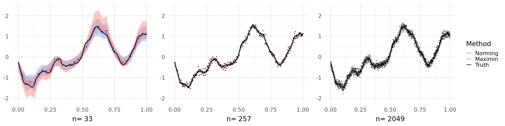
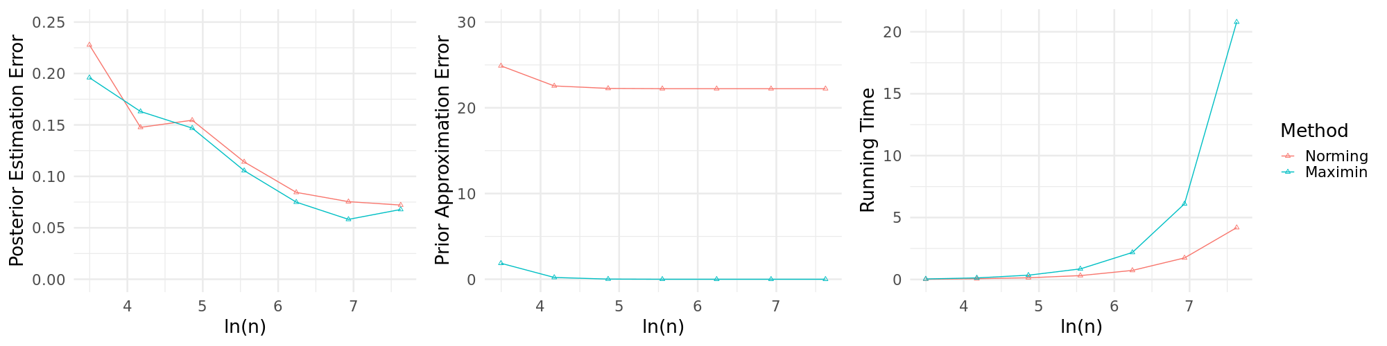
We illustrate the nonparametric regression with Vecchia GPs in Figure 3. Both Vecchia GP methods show similar performances, with relatively large estimation error and wide credible bands when sample size is small ($n=33$), but can estimate the true function perfectly well as sample size becomes large enough ($n=2049$). Figure 4 provides more qualitative reports of the two Vecchia GPs in view of estimation accuracy, prior approximation and run time. The estimation error is measured by the $\ell^{\infty}$ distance between the posterior mean and the true regression function. As sample size $n$ increases, both Vecchia GP methods recover the true regression function well in supremum norm, with errors not exceeding $0.075$. The prior approximation error is measured by the squared Wasserstein-2 distance between the marginal distributions of the Vecchia GP and the corresponding mother GP on $\mathcal{X}_{n}$. As we can see, the Vecchia GP with Layered Norming DAG does not approximate the mother GP well. In fact the squared Wasserstein-2 distance doesn’t go below $20$ for any sample size $n$, while the Vecchia GP with maximin ordering has squared Wasserstein-2 distance tending to zero. In view of the posterior estimation and prior approximation results, it is evident that Vecchia GPs do not require close approximation of the corresponding mother GPs, to recover the true function.

We also plot the computation times of two Vecchia GPs on the right side of Figure 4. Since the Vecchia GPs with Layered Norming DAGs have fixed cardinality $2$ for all parent sets while NNGP with Maximin ordering has parent sets of size $2\ln n$, it is intuitively clear that the former can be computed much faster than the later. The difference in the runtime increases with the sample size. Therefore, if the objective is nonparametric inference of the underlying function, we can employ Vecchia GPs with extremely small parent size ($2$ in this example), exploiting the computational benefits without loss of statistical efficiency.

Refer to caption
Figure 3: Illustration of Nonparametric Regression with Vecchia GPs. Black lines and dots denote true regression function and observed data, respectively. Colored line and regions denote posterior mean and $95\%$ credible intervals from two Vecchia GP methods.
Refer to caption
Figure 4: Qualitative results of applying two Vecchia GP methods under different sample sizes. Left: posterior estimation error measured by $\ell^{\infty}$ norm between the truth and the posterior mean; Middle: prior approximation error measured by squared Wasserstein distance between marginals of Vecchia GPs and their mother GPs; Right: Run time of MCMC inference measured by seconds.

6.2 Norming Sets

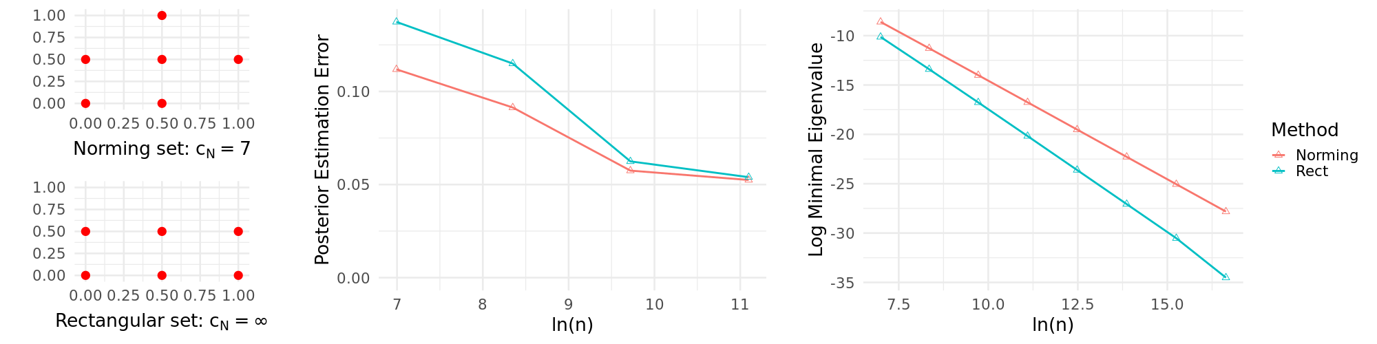
In view of our theoretical results, norming parent sets are sufficient to guarantee optimal estimation rates. In this section, we investigate the necessity of choosing norming sets. We keep all other aspects of the models fixed and compare DAGs with norming sets and non-norming sets as parents. We demonstrate numerically that the violation of the norming sets condition negatively affects the empirical performance of Vecchia GP methods. Since in a unidimensional space, all sets with distinct elements are norming sets, we consider the unit square $[0,1]^{2}$ as domain and set $\mathcal{X}_{n}$ to be a grid on it. We set the true regression function generating the data as $f_{0}(x)=2(x[1]-0.5)^{2}+4(x[2]-0.5)^{2}+x[1]x[2]^{2}.$ The mother Gaussian process is a Matérn process with smoothness parameter $\alpha=5/2$ and scaling parameters $\tau=8,s=1$. We consider Vecchia GPs with two DAG structures in the comparison. The first is the Layered Norming DAG with $\underline{\alpha}=2$ and norming sets of cardinality ${\underline{\alpha}+d\choose\underline{\alpha}}=6$. The second DAG is almost identical to the first except we intentionally choose all parent sets NOT to form a norming sets. All these parent sets have identical geometric shapes as shown in the left plot of Figure 5. Since the elements form a rectangle, we name these DAGs as Rectangle DAGs (denoted as “Rect” in the figures).

We compare Vecchia GPs with Layered Norming DAGs and Rectangle DAGs from two perspectives. We consider both the posterior estimation error and the computational stability in large sample sizes, see Figure 5. Since they both approximate their mother GPs poorly and have almost the same computational time, we do not display these quantities. Inspecting the figure, one can observe that Vecchia GPs with Norming DAGs perform consistently better for estimation than Rectangle DAGs. In view of our theoretical results, the differences in the approximation accuracy stems from using all quadratic polynomials (Norming DAGs) versus a subspace of them (Rectangle DAGs). Specifically, the norming set in the left plot of Figure 5 uniquely determines all functions in the linear space

$$\mathcal{P}_{2}(\Omega)=\mathrm{span}\{1,x[1],x[2],x[1]^{2},x[1]x[2],x[2]^{2}\},$$

while the rectangle set in this plot only uniquely determines functions in the space

$$\tilde{\mathcal{P}}_{2}(\Omega)=\mathrm{span}\{1,x[1],x[2],x[1]^{2},x[1]x[2]\}.$$

The latter does not include quadratic forms of $x[2]$, which resulting in large estimation error for the true function, which is twice differentiable in $x[2]$.

The other issue with the non-norming sets is the numerical instability for large sample sizes, or in other words, the instability in the flat limit. In view of equations (2.2) and (2.2), computing the conditional distributions of Vecchia GPs involves the inversion of the Matérn covariance matrix $K_{\mathrm{pa}(X_{i}),\mathrm{pa}(X_{i})}$ for all $X_{i}\in\mathcal{X}_{n}$. However, as $n$ increases, the eigenvalues might get close to zero, rendering the problem numerically unstable. To demonstrate this we plot the minimal eigenvalues of the matrices $K_{\mathrm{pa}(X_{i}),\mathrm{pa}(X_{i})}$ among all locations $X_{i}\in\mathcal{X}_{n}$ on the right hand side of Figure 5. One can observe that the difference between the two methods is substantial. For example in case of $n=4,198,401$, the minimal eigenvalue of the Rectangle DAG is $1/238$ of the Norming DAG. In fact, the Rectangle DAGs have significantly smaller minimal eigenvalues for all sample sizes, and reaches numerical singularity much faster than the Norming DAGs. Recall that in Section 4.2 all results regarding the flat limit of Matérn processes require the parent sets to be a norming sets. It is unclear whether the flat limits exist and in case yes, how they look like in case the norming condition is violated. Our numerical results, however, pose a warning in such cases.

Refer to caption
Figure 5: Comparison between the Layered Norming DAGs and Rectangle (non-norming) DAGs for different sample sizes. Left: geometric shaps of the norming and the rectangular (non-norming) sets; Middle: $\ell^{\infty}$ distance between the truth and the posterior mean; Right: infimum over $X_{i}$ of the logarithm of the minimal eigenvalues of the matrix $K_{\mathrm{pa}(X_{i}),\mathrm{pa}(X_{i})}$ among all $X_{i}\in\mathcal{X}_{n}$.

7 Discussion

7.1 Statistical Guarantees of Approximation Methods

Vecchia approximations of Gaussian processes have become popular in the past ten years due to its scalability to huge datasets. However, the developments of statistical guarantees for Vecchia GPs is relatively slow compared to their wide applications. Previous works focused mostly on the approximation properties of the Vecchia GPs to the mother Gaussian processes rather than looking at them as standalone processes. Therefore, the existing, sparse literature on the statistical guarantees of Vecchia GPs are built on the prerequisite that the approximation error (measured in some metrics, e.g., Wasserstein distance or KL divergence) between Vecchia GPs and the corresponding mother GPs are small enough. Although this strategy is also sound, in principle might lead to suboptimal result in requiring close proximity to the original GP, which is not necessary for optimal statistical inference. In fact, Vecchia GPs can have fundamentally different properties than the corresponding mother GPs. For instance the popular Matérn process is stationary, while this property is not inherited by the Vecchia approximation. Our paper therefore derived fundamental probabilistic (e.g. centered and de-centered small ball probabilities) and statistical properties (e.g contraction rates of the posterior) of Vecchia GPs, which so far haven’t been studied in the literature.

7.2 Polynomials and Vecchia GPs

One of the fundamental contributions of our paper is the description of Vecchia GPs with the help of polynomial interpolations. In fact, Theorem 1 and Lemma 6 show, that under mild conditions, Matérn GPs, as well as their Vecchia approximations, can be well characterized by polynomials when conditioned on a norming set. Moreover, the cardinality of the norming set is the same as the dimensionality of the vector space spawned by certain polynomials. For the Matérn Gaussian process with regularity $\alpha$, this vector space is the collection of polynomials with order bounded by $\underline{\alpha}$, which has cardinality ${\underline{\alpha}+d\choose\underline{\alpha}}$. This implies, that regardless of the sample size $n$, a finite, well chosen parent set is sufficient. This makes Vecchia GPs highly scalable to large datasets.

Apart from the fixed cardinality, norming sets also have some unique geometrical properties. Intuitively speaking, elements in a norming sets need to fully express the local geometry of polynomials up to certain order. While this is trivia in the unidimensional space, it becomes highly challenging in high-dimensional spaces. Specifically, as illustrated in Figure 2, sets with different geometric shapes can have vastly different norming constants. It is even possible to find sets consisting of close by points which are not norming. This partially explains why remote locations were proposed as parent sets [3]. In fact, finding norming sets and controlling the associated norming constants is a difficult problem. In most cases, the norming constants are evaluated only numerically, with only a few analytic exceptions, e.g. the Fekete points studied by [8].

{acks}

[Acknowledgments] The authors would like to thank Yuansi Chen, Zichao Dong, Cheng Li, Andy MarCormack, Galen Reeves, Bernhard Stankewitz and Dun Tang for helpful discussion. The authors also thank Michele Peruzzi for access to computation resources.

{funding}

The authors are funded by European Research Council on the project: “BigBayesUQ: The missing story of Bayesian uncertainty quantification for big data” with grant No. 101041064.

{supplement}\stitle

Supplementary Materials to “Vecchia Gaussian Processes: Probabilistic Properties, Minimax Rates and Methodological Developments” \sdescriptionProofs for Theorems, Lemmas and Corollaries that appear in the main paper. {supplement} \stitlePackage “GPDAG”: https://github.com/yi-chen-zhu/GPDAG \sdescriptionR package for Bayesian posterior inference of Gaussian processes with generic DAG structures, including the Layered Norming DAG proposed by this paper. This repository also includes the codes for numerical studies.

References

  • [1] {barticle}[author] \bauthor\bsnmAurzada, \bfnmFrank\binitsF., \bauthor\bsnmIbragimov, \bfnmIldar A\binitsI. A., \bauthor\bsnmLifshits, \bfnmMA\binitsM. and \bauthor\bsnmVan Zanten, \bfnmJH\binitsJ. (\byear2009). \btitleSmall deviations of smooth stationary Gaussian processes. \bjournalTheory of Probability & Its Applications \bvolume53 \bpages697–707. \endbibitem
  • [2] {barticle}[author] \bauthor\bsnmBai, \bfnmYun\binitsY., \bauthor\bsnmSong, \bfnmPeter X-K\binitsP. X.-K. and \bauthor\bsnmRaghunathan, \bfnmTE\binitsT. (\byear2012). \btitleJoint composite estimating functions in spatiotemporal models. \bjournalJournal of the Royal Statistical Society Series B: Statistical Methodology \bvolume74 \bpages799–824. \endbibitem
  • [3] {bbook}[author] \bauthor\bsnmBanerjee, \bfnmSudipto\binitsS., \bauthor\bsnmCarlin, \bfnmBradley P\binitsB. P. and \bauthor\bsnmGelfand, \bfnmAlan E\binitsA. E. (\byear2015). \btitleHierarchical modeling and analysis for spatial data. \bpublisherChapman and Hall/CRC. \endbibitem
  • [4] {barticle}[author] \bauthor\bsnmBanerjee, \bfnmSudipto\binitsS., \bauthor\bsnmGelfand, \bfnmAlan E\binitsA. E., \bauthor\bsnmFinley, \bfnmAndrew O\binitsA. O. and \bauthor\bsnmSang, \bfnmHuiyan\binitsH. (\byear2008). \btitleGaussian predictive process models for large spatial data sets. \bjournalJournal of the Royal Statistical Society Series B: Statistical Methodology \bvolume70 \bpages825–848. \endbibitem
  • [5] {barticle}[author] \bauthor\bsnmBevilacqua, \bfnmMoreno\binitsM. and \bauthor\bsnmGaetan, \bfnmCarlo\binitsC. (\byear2015). \btitleComparing composite likelihood methods based on pairs for spatial Gaussian random fields. \bjournalStatistics and Computing \bvolume25 \bpages877–892. \endbibitem
  • [6] {barticle}[author] \bauthor\bsnmBhatt, \bfnmSamir\binitsS., \bauthor\bsnmWeiss, \bfnmDJ\binitsD., \bauthor\bsnmCameron, \bfnmE\binitsE., \bauthor\bsnmBisanzio, \bfnmD\binitsD., \bauthor\bsnmMappin, \bfnmB\binitsB., \bauthor\bsnmDalrymple, \bfnmU\binitsU., \bauthor\bsnmBattle, \bfnmKE\binitsK., \bauthor\bsnmMoyes, \bfnmCL\binitsC., \bauthor\bsnmHenry, \bfnmA\binitsA., \bauthor\bsnmEckhoff, \bfnmPA\binitsP. \betalet al. (\byear2015). \btitleThe effect of malaria control on Plasmodium falciparum in Africa between 2000 and 2015. \bjournalNature \bvolume526 \bpages207–211. \endbibitem
  • [7] {barticle}[author] \bauthor\bsnmBorell, \bfnmChrister\binitsC. (\byear1975). \btitleThe brunn-minkowski inequality in gauss space. \bjournalInventiones mathematicae \bvolume30 \bpages207–216. \endbibitem
  • [8] {barticle}[author] \bauthor\bsnmBos, \bfnmLen\binitsL. (\byear2018). \btitleFekete points as norming sets. \bjournalDolomites Research Notes on Approximation \bvolume11 \bpages26–34. \endbibitem
  • [9] {barticle}[author] \bauthor\bsnmCao, \bfnmJian\binitsJ., \bauthor\bsnmGuinness, \bfnmJoseph\binitsJ., \bauthor\bsnmGenton, \bfnmMarc G\binitsM. G. and \bauthor\bsnmKatzfuss, \bfnmMatthias\binitsM. (\byear2022). \btitleScalable Gaussian-process regression and variable selection using Vecchia approximations. \bjournalJournal of machine learning research \bvolume23 \bpages1–30. \endbibitem
  • [10] {barticle}[author] \bauthor\bsnmCressie, \bfnmNoel\binitsN. and \bauthor\bsnmJohannesson, \bfnmGardar\binitsG. (\byear2008). \btitleFixed rank kriging for very large spatial data sets. \bjournalJournal of the Royal Statistical Society Series B: Statistical Methodology \bvolume70 \bpages209–226. \endbibitem
  • [11] {bbook}[author] \bauthor\bsnmCressie, \bfnmNoel\binitsN. and \bauthor\bsnmWikle, \bfnmChristopher K\binitsC. K. (\byear2011). \btitleStatistics for spatio-temporal data. \bpublisherJohn Wiley & Sons. \endbibitem
  • [12] {barticle}[author] \bauthor\bsnmDatta, \bfnmAbhirup\binitsA., \bauthor\bsnmBanerjee, \bfnmSudipto\binitsS., \bauthor\bsnmFinley, \bfnmAndrew O\binitsA. O. and \bauthor\bsnmGelfand, \bfnmAlan E\binitsA. E. (\byear2016). \btitleHierarchical nearest-neighbor Gaussian process models for large geostatistical datasets. \bjournalJournal of the American Statistical Association \bvolume111 \bpages800–812. \endbibitem
  • [13] {binproceedings}[author] \bauthor\bsnmDaxberger, \bfnmErik A\binitsE. A. and \bauthor\bsnmLow, \bfnmBryan Kian Hsiang\binitsB. K. H. (\byear2017). \btitleDistributed batch Gaussian process optimization. In \bbooktitleInternational conference on machine learning \bpages951–960. \bpublisherPMLR. \endbibitem
  • [14] {binproceedings}[author] \bauthor\bsnmDeisenroth, \bfnmMarc\binitsM. and \bauthor\bsnmNg, \bfnmJun Wei\binitsJ. W. (\byear2015). \btitleDistributed Gaussian processes. In \bbooktitleInternational conference on machine learning \bpages1481–1490. \bpublisherPMLR. \endbibitem
  • [15] {barticle}[author] \bauthor\bsnmDriscoll, \bfnmTobin A\binitsT. A. and \bauthor\bsnmFornberg, \bfnmBengt\binitsB. (\byear2002). \btitleInterpolation in the limit of increasingly flat radial basis functions. \bjournalComputers & Mathematics with Applications \bvolume43 \bpages413–422. \endbibitem
  • [16] {barticle}[author] \bauthor\bsnmFurrer, \bfnmReinhard\binitsR., \bauthor\bsnmGenton, \bfnmMarc G\binitsM. G. and \bauthor\bsnmNychka, \bfnmDouglas\binitsD. (\byear2006). \btitleCovariance tapering for interpolation of large spatial datasets. \bjournalJournal of Computational and Graphical Statistics \bvolume15 \bpages502–523. \endbibitem
  • [17] {barticle}[author] \bauthor\bsnmGasca, \bfnmMariano\binitsM. and \bauthor\bsnmSauer, \bfnmThomas\binitsT. (\byear2000). \btitlePolynomial interpolation in several variables. \bjournalAdvances in Computational Mathematics \bvolume12 \bpages377–410. \endbibitem
  • [18] {bincollection}[author] \bauthor\bsnmGasca, \bfnmMariano\binitsM. and \bauthor\bsnmSauer, \bfnmThomas\binitsT. (\byear2001). \btitleOn the history of multivariate polynomial interpolation. In \bbooktitleNumerical Analysis: Historical Developments in the 20th Century \bpages135–147. \bpublisherElsevier. \endbibitem
  • [19] {bbook}[author] \bauthor\bsnmGelfand, \bfnmAlan E\binitsA. E., \bauthor\bsnmDiggle, \bfnmPeter\binitsP., \bauthor\bsnmGuttorp, \bfnmPeter\binitsP. and \bauthor\bsnmFuentes, \bfnmMontserrat\binitsM. (\byear2010). \btitleHandbook of spatial statistics. \bpublisherCRC press. \endbibitem
  • [20] {barticle}[author] \bauthor\bsnmGelfand, \bfnmAlan E\binitsA. E. and \bauthor\bsnmSchliep, \bfnmErin M\binitsE. M. (\byear2016). \btitleSpatial statistics and Gaussian processes: A beautiful marriage. \bjournalSpatial Statistics \bvolume18 \bpages86–104. \endbibitem
  • [21] {barticle}[author] \bauthor\bsnmGhosal, \bfnmSubhashis\binitsS., \bauthor\bsnmGhosh, \bfnmJayanta K\binitsJ. K. and \bauthor\bsnmVan Der Vaart, \bfnmAad W\binitsA. W. (\byear2000). \btitleConvergence rates of posterior distributions. \bjournalAnnals of Statistics \bpages500–531. \endbibitem
  • [22] {bbook}[author] \bauthor\bsnmGhosal, \bfnmSubhashis\binitsS. and \bauthor\bparticleVan der \bsnmVaart, \bfnmAad\binitsA. (\byear2017). \btitleFundamentals of nonparametric Bayesian inference \bvolume44. \bpublisherCambridge University Press. \endbibitem
  • [23] {bbook}[author] \bauthor\bsnmGrafakos, \bfnmLoukas\binitsL. (\byear2014). \btitleClassical fourier analysis \bvolume2. \bpublisherSpringer. \endbibitem
  • [24] {barticle}[author] \bauthor\bsnmGuinness, \bfnmJoseph\binitsJ. (\byear2018). \btitlePermutation and grouping methods for sharpening Gaussian process approximations. \bjournalTechnometrics \bvolume60 \bpages415–429. \endbibitem
  • [25] {barticle}[author] \bauthor\bsnmJetter, \bfnmKurt\binitsK., \bauthor\bsnmStöckler, \bfnmJoachim\binitsJ. and \bauthor\bsnmWard, \bfnmJoseph\binitsJ. (\byear1999). \btitleError estimates for scattered data interpolation on spheres. \bjournalMathematics of Computation \bvolume68 \bpages733–747. \endbibitem
  • [26] {barticle}[author] \bauthor\bsnmKang, \bfnmMyeongjong\binitsM., \bauthor\bsnmSchäfer, \bfnmFlorian\binitsF., \bauthor\bsnmGuinness, \bfnmJoseph\binitsJ. and \bauthor\bsnmKatzfuss, \bfnmMatthias\binitsM. (\byear2024). \btitleAsymptotic properties of Vecchia approximation for Gaussian processes. \bjournalarXiv preprint arXiv:2401.15813. \endbibitem
  • [27] {barticle}[author] \bauthor\bsnmKatzfuss, \bfnmMatthias\binitsM. and \bauthor\bsnmGuinness, \bfnmJoseph\binitsJ. (\byear2021). \btitleA general framework for Vecchia approximations of Gaussian processes. \bjournalStatistical Science \bvolume36 \bpages124–141. \endbibitem
  • [28] {barticle}[author] \bauthor\bsnmKatzfuss, \bfnmMatthias\binitsM., \bauthor\bsnmGuinness, \bfnmJoseph\binitsJ., \bauthor\bsnmGong, \bfnmWenlong\binitsW. and \bauthor\bsnmZilber, \bfnmDaniel\binitsD. (\byear2020). \btitleVecchia approximations of Gaussian-process predictions. \bjournalJournal of Agricultural, Biological and Environmental Statistics \bvolume25 \bpages383–414. \endbibitem
  • [29] {barticle}[author] \bauthor\bsnmKaufman, \bfnmCari G\binitsC. G., \bauthor\bsnmSchervish, \bfnmMark J\binitsM. J. and \bauthor\bsnmNychka, \bfnmDouglas W\binitsD. W. (\byear2008). \btitleCovariance tapering for likelihood-based estimation in large spatial data sets. \bjournalJournal of the American Statistical Association \bvolume103 \bpages1545–1555. \endbibitem
  • [30] {barticle}[author] \bauthor\bsnmKuelbs, \bfnmJames\binitsJ., \bauthor\bsnmLi, \bfnmWenbo V\binitsW. V. and \bauthor\bsnmLinde, \bfnmWerner\binitsW. (\byear1994). \btitleThe Gaussian measure of shifted balls. \bjournalProbability Theory and Related Fields \bvolume98 \bpages143–162. \endbibitem
  • [31] {barticle}[author] \bauthor\bsnmKündig, \bfnmPascal\binitsP. and \bauthor\bsnmSigrist, \bfnmFabio\binitsF. (\byear2023). \btitleIterative Methods for Vecchia-Laplace Approximations for Latent Gaussian Process Models. \bjournalJournal of American Statistical Association \bvolumeto appear. \endbibitem
  • [32] {barticle}[author] \bauthor\bsnmLaakso, \bfnmT. I.\binitsT. I., \bauthor\bsnmValimaki, \bfnmV.\binitsV., \bauthor\bsnmKarjalainen, \bfnmM.\binitsM. and \bauthor\bsnmLaine, \bfnmU. K.\binitsU. K. (\byear1996). \btitleSplitting the unit delay [FIR/all pass filters design]. \bjournalIEEE Signal Processing Magazine \bvolume13 \bpages30-60. \endbibitem
  • [33] {barticle}[author] \bauthor\bsnmLarsson, \bfnmElisabeth\binitsE. and \bauthor\bsnmFornberg, \bfnmBengt\binitsB. (\byear2005). \btitleTheoretical and computational aspects of multivariate interpolation with increasingly flat radial basis functions. \bjournalComputers & Mathematics with Applications \bvolume49 \bpages103–130. \endbibitem
  • [34] {barticle}[author] \bauthor\bsnmLedoux, \bfnmMichel\binitsM. (\byear2006). \btitleIsoperimetry and Gaussian analysis. \bjournalLectures on Probability Theory and Statistics: Ecole d’Eté de Probabilités de Saint-Flour XXIV—1994 \bpages165–294. \endbibitem
  • [35] {barticle}[author] \bauthor\bsnmLee, \bfnmJaehoon\binitsJ., \bauthor\bsnmBahri, \bfnmYasaman\binitsY., \bauthor\bsnmNovak, \bfnmRoman\binitsR., \bauthor\bsnmSchoenholz, \bfnmSamuel S\binitsS. S., \bauthor\bsnmPennington, \bfnmJeffrey\binitsJ. and \bauthor\bsnmSohl-Dickstein, \bfnmJascha\binitsJ. (\byear2017). \btitleDeep neural networks as Gaussian processes. \bjournalarXiv preprint arXiv:1711.00165. \endbibitem
  • [36] {barticle}[author] \bauthor\bsnmLee, \bfnmYeon Ju\binitsY. J., \bauthor\bsnmMicchelli, \bfnmCharles A\binitsC. A. and \bauthor\bsnmYoon, \bfnmJungho\binitsJ. (\byear2015). \btitleA study on multivariate interpolation by increasingly flat kernel functions. \bjournalJournal of Mathematical Analysis and Applications \bvolume427 \bpages74–87. \endbibitem
  • [37] {barticle}[author] \bauthor\bsnmLi, \bfnmWenbo V.\binitsW. V. and \bauthor\bsnmLinde, \bfnmWerner\binitsW. (\byear1999). \btitleApproximation, Metric Entropy and Small Ball Estimates for Gaussian Measures. \bjournalThe Annals of Probability \bvolume27 \bpages1556 – 1578. \endbibitem
  • [38] {barticle}[author] \bauthor\bsnmLi, \bfnmWenbo V\binitsW. V. and \bauthor\bsnmShao, \bfnmQ-M\binitsQ.-M. (\byear2001). \btitleGaussian processes: inequalities, small ball probabilities and applications. \bjournalHandbook of Statistics \bvolume19 \bpages533–597. \endbibitem
  • [39] {barticle}[author] \bauthor\bsnmLiu, \bfnmHaitao\binitsH., \bauthor\bsnmOng, \bfnmYew-Soon\binitsY.-S., \bauthor\bsnmShen, \bfnmXiaobo\binitsX. and \bauthor\bsnmCai, \bfnmJianfei\binitsJ. (\byear2020). \btitleWhen Gaussian process meets big data: A review of scalable GPs. \bjournalIEEE transactions on neural networks and learning systems \bvolume31 \bpages4405–4423. \endbibitem
  • [40] {barticle}[author] \bauthor\bsnmNeidinger, \bfnmRichard D\binitsR. D. (\byear2019). \btitleMultivariate polynomial interpolation in Newton forms. \bjournalSIAM Review \bvolume61 \bpages361–381. \endbibitem
  • [41] {bmisc}[author] \bauthor\bsnmOlver, \bfnmF. W. J.\binitsF. W. J., \bauthor\bsnmDaalhuis, \bfnmA. B. Olde\binitsA. B. O., \bauthor\bsnmLozier, \bfnmD. W.\binitsD. W., \bauthor\bsnmSchneider, \bfnmB. I.\binitsB. I., \bauthor\bsnmBoisvert, \bfnmR. F.\binitsR. F., \bauthor\bsnmClark, \bfnmC. W.\binitsC. W., \bauthor\bsnmB. R. Mille and, \bfnmB. V. Saunders\binitsB. V. S., \bauthor\bsnmCohl, \bfnmH. S.\binitsH. S. and \bauthor\bsnmM. A. McClain, \bfnmeds.\binitse. (\byear2024). \btitleNIST Digital Library of Mathematical Functions. \bhowpublishedhttp://dlmf.nist.gov/, Release 1.2.1 of 2024-06-15. \endbibitem
  • [42] {barticle}[author] \bauthor\bsnmPeruzzi, \bfnmMichele\binitsM., \bauthor\bsnmBanerjee, \bfnmSudipto\binitsS. and \bauthor\bsnmFinley, \bfnmAndrew O\binitsA. O. (\byear2022). \btitleHighly scalable Bayesian geostatistical modeling via meshed Gaussian processes on partitioned domains. \bjournalJournal of the American Statistical Association \bvolume117 \bpages969–982. \endbibitem
  • [43] {barticle}[author] \bauthor\bsnmQuinonero-Candela, \bfnmJoaquin\binitsJ. and \bauthor\bsnmRasmussen, \bfnmCarl Edward\binitsC. E. (\byear2005). \btitleA unifying view of sparse approximate Gaussian process regression. \bjournalThe Journal of Machine Learning Research \bvolume6 \bpages1939–1959. \endbibitem
  • [44] {barticle}[author] \bauthor\bsnmSchäfer, \bfnmFlorian\binitsF., \bauthor\bsnmSullivan, \bfnmTimothy John\binitsT. J. and \bauthor\bsnmOwhadi, \bfnmHouman\binitsH. (\byear2021). \btitleCompression, inversion, and approximate PCA of dense kernel matrices at near-linear computational complexity. \bjournalMultiscale Modeling & Simulation \bvolume19 \bpages688–730. \endbibitem
  • [45] {barticle}[author] \bauthor\bsnmSeeger, \bfnmMatthias\binitsM. (\byear2004). \btitleGaussian processes for machine learning. \bjournalInternational journal of neural systems \bvolume14 \bpages69–106. \endbibitem
  • [46] {barticle}[author] \bauthor\bsnmSong, \bfnmGuohui\binitsG., \bauthor\bsnmRiddle, \bfnmJohn\binitsJ., \bauthor\bsnmFasshauer, \bfnmGregory E\binitsG. E. and \bauthor\bsnmHickernell, \bfnmFred J\binitsF. J. (\byear2012). \btitleMultivariate interpolation with increasingly flat radial basis functions of finite smoothness. \bjournalAdvances in Computational Mathematics \bvolume36 \bpages485–501. \endbibitem
  • [47] {barticle}[author] \bauthor\bsnmStein, \bfnmMichael L\binitsM. L. (\byear2013). \btitleStatistical properties of covariance tapers. \bjournalJournal of Computational and Graphical Statistics \bvolume22 \bpages866–885. \endbibitem
  • [48] {barticle}[author] \bauthor\bsnmSzabó, \bfnmBotond\binitsB., \bauthor\bsnmHadji, \bfnmAmine\binitsA. and \bauthor\bparticlevan der \bsnmVaart, \bfnmAad\binitsA. (\byear2023). \btitleAdaptation using spatially distributed Gaussian Processes. \bjournalarXiv preprint arXiv:2312.14130. \endbibitem
  • [49] {barticle}[author] \bauthor\bsnmSzabó, \bfnmBotond\binitsB. and \bauthor\bsnmVan Zanten, \bfnmHarry\binitsH. (\byear2019). \btitleAn asymptotic analysis of distributed nonparametric methods. \bjournalJournal of Machine Learning Research \bvolume20 \bpages1–30. \endbibitem
  • [50] {binproceedings}[author] \bauthor\bsnmTitsias, \bfnmM.\binitsM. (\byear2009). \btitleVariational Learning of Inducing Variables in Sparse Gaussian Processes. In \bbooktitleProceedings of the 12th International Conference on Artificial Intelligence and Statistics \bvolume5 \bpages567–574. \bpublisherPMLR. \endbibitem
  • [51] {barticle}[author] \bauthor\bparticlevan der \bsnmVaart, \bfnmAad\binitsA. and \bauthor\bparticlevan \bsnmZanten, \bfnmHarry\binitsH. (\byear2011). \btitleInformation Rates of Nonparametric Gaussian Process Methods. \bjournalJournal of Machine Learning Research \bvolume12 \bpages2095–2119. \endbibitem
  • [52] {barticle}[author] \bauthor\bparticlevan der \bsnmVaart, \bfnmAad W\binitsA. W. and \bauthor\bparticlevan \bsnmZanten, \bfnmJ Harry\binitsJ. H. (\byear2008). \btitleRates of contraction of posterior distributions based on Gaussian process priors. \endbibitem
  • [53] {barticle}[author] \bauthor\bsnmVecchia, \bfnmAldo V\binitsA. V. (\byear1988). \btitleEstimation and model identification for continuous spatial processes. \bjournalJournal of the Royal Statistical Society Series B: Statistical Methodology \bvolume50 \bpages297–312. \endbibitem
  • [54] {bbook}[author] \bauthor\bsnmWendland, \bfnmHolger\binitsH. (\byear2004). \btitleScattered data approximation \bvolume17. \bpublisherCambridge university press. \endbibitem
  • [55] {bbook}[author] \bauthor\bsnmWilliams, \bfnmChristopher KI\binitsC. K. and \bauthor\bsnmRasmussen, \bfnmCarl Edward\binitsC. E. (\byear2006). \btitleGaussian processes for machine learning \bvolume2. \bpublisherMIT press Cambridge, MA. \endbibitem
  • [56] {barticle}[author] \bauthor\bsnmZhang, \bfnmLu\binitsL., \bauthor\bsnmTang, \bfnmWenpin\binitsW. and \bauthor\bsnmBanerjee, \bfnmSudipto\binitsS. (\byear2023). \btitleFixed-Domain Asymptotics Under Vecchia’s Approximation of Spatial Process Likelihoods. \bjournalarXiv preprint arXiv:2101.08861. \endbibitem
  • [57] {barticle}[author] \bauthor\bsnmZhu, \bfnmYichen\binitsY., \bauthor\bsnmPeruzzi, \bfnmMichele\binitsM., \bauthor\bsnmLi, \bfnmCheng\binitsC. and \bauthor\bsnmDunson, \bfnmDavid B\binitsD. B. (\byear2024). \btitleRadial neighbours for provably accurate scalable approximations of Gaussian processes. \bjournalBiometrika \bpagesasae029. \endbibitem

and

The supplementary materials contain proofs for all theorems, lemmas and corollaries, as well as algorithms in the main paper. For all proofs from Section B.2 and onwards, we only prove the case for $\alpha\not\in\mathbb{N}$. The case where $\alpha$ being integers can be easily obtained by including a logarithm terms in all relevant formulas.

A Proofs of the lemmas and Algorithms in Section 3

A.1 Proof of Lemma 1

Proof.

First note, that in case the Vandermonde matrix $V_{A}$ is invertible, then equation (15) provides a solution to the polynomial interpolation problem.

We prove the “if and only if” statement by contradiction. Suppose the Vandermonde matrix $V_{A}$ is not invertible. Because $V_{A}$ is a square matrix, there exists a vector $b\neq 0$, such that $V_{A}b=0$. Assume furthermore that there exists a polynomial $P(x)$ satisfying ${P}(w_{i})=y_{i},\forall 1\leq i\leq m$, otherwise the statement holds. Then the polynomial $\tilde{P}(x)=P(x)+\sum_{i=1}^{m}b[i]x^{k_{(i)}}$ also satisfies $\tilde{P}(w_{i})=y_{i},\forall 1\leq i\leq m$, hence in view of $b\neq 0$, there are at least two solutions to the interpolation problem.

On the other hand, suppose the polynomial interpolation problem is not unisolvent. If there is no solution, then the matrix $V_{A}$ can not be invertible, otherwise equation (15) claims a solution. Else, if there are at least two polynomials $P_{1}\neq P_{2}$ satisfying $P_{j}(w_{i})=y_{i},j=1,2$, then we have $P_{1}-P_{2}\neq 0$ and $(P_{1}-P_{2})(w_{i})=0,\forall 1\leq i\leq m$. Let us write the difference in the form $(P_{1}-P_{2})(x)=\sum_{i=1}^{m}b[i]x^{k_{(i)}}$ and collect the coefficients in the vector $b=(b[1],b[2],\cdots,b[m])^{T}$. Note that since $b\neq 0$ and $V_{A}b=0$, the matrix $V_{A}$ is not invertible.

Finally, since we have proved the unisolvency is equivalent to $V_{A}$ being invertible and equation (15) provides a solution to the polynomial interpoaltion problem, this solution is also the unique solution. ∎

A.2 Proof of Lemma 2

Proof.

We first prove (2) $\Rightarrow$ (1). Since the smallest singular value of the Vandermonde matrix $V_{A}$ is positive, the matrix $V_{A}$ is invertible. By Lemma 1, the set $A$ is unisolvent with respect to $\mathscr{P}_{l}(\mathbb{R}^{d})$ and hence also unisolvent for $\mathscr{P}_{l}(\Omega)$. Therefore, for all polynomials $P\in\mathscr{P}_{l}(\mathbb{R}^{d})$, we have

$$P(x)=P(A)^{T}V_{A}^{-1}v_{x}.$$ (40)

This allows us to control $P(x),\;\forall x\in\Omega$ as

$\displaystyle|P(x)|\leq$ $\displaystyle\|P(A)\|_{2}\|V_{A}^{-1}\|_{2}\|v_{x}\|_{2}\leq\sqrt{m}\max_{x^{\prime}\in A}|P(x^{\prime})|\cdot c_{S}^{-1}\cdot\sqrt{m}\leq{l+d\choose l}c_{S}^{-1}\max_{x^{\prime}\in A}|P(x^{\prime})|,$

where we utilizes $\|v_{x}\|_{2}\leq\sqrt{m}$ for $x\in\Omega=[0,1]^{d}$. Thus, $A$ is a norming set with norming constant

$$c_{N}\leq{l+d\choose l}c_{S}^{-1}.$$

We proceed to prove (1) $\Rightarrow$ (2). First we prove by contradiction that the matrix $V_{A}$ is invertible. Assume that this is not true. Then there exists a non-zero vector $b\in\mathbb{R}^{m}$, such that $V_{A}^{T}b=0$. Consider the polynomial $P(x)=b^{T}v_{x}\in\mathcal{P}_{l}(\Omega)$. In view of $V_{A}^{T}b=0$, we have $\sum_{i=1}^{m}b[i]x^{k_{(i)}}=0$, for all $x\in A$, i.e. $\|P\|_{A}=0$. However, $b$ is a nonzero vector, hence there exists $x^{\prime}\in\Omega$, such that $P(x^{\prime})\neq 0$, i.e. $\sup_{x}|P(x)|>0$. This contradicts to $A$ being a norming set. Hence matrix $V_{A}$ must be invertible. Then as proved in Lemma 1, for all polynomials $P\in\mathscr{P}_{l}(\Omega)$, equation (40) holds.

Next let us introduce a “standard” norming set to facilitate the connection of the constants $c_{S}$ and $c_{N}$. Define the set $A^{*}$ as

$$A^{*}=\{(x\in\mathbb{R}^{d}:x[i]\in\{0/l,1/l,\cdots,l/l\},\forall 1\leq i\leq d;\|x\|_{1}\leq 1\}.$$

The set $A^{*}$ is a “corner” set as in Section 3 of [40] with cardinality $m={l+d\choose l}$ and is unisolvent. Denote the minimal singular value of $V_{A^{*}}$ by $c^{*}$. Then for all $u\in\mathbb{R}^{m}$ with $\|u\|_{2}=1$,

$$c^{*}\leq\|u^{T}V_{A^{*}}\|_{2}=\sqrt{\sum_{x^{\prime}\in A^{*}}(v_{x^{\prime}}^{T}u)^{2}}\leq\sqrt{m}\sup_{x^{\prime}\in A^{*}}|v_{x^{\prime}}^{T}u|\leq\sqrt{m}\sup_{x\in\Omega}|v_{x}^{T}u|.$$

Therefore, for all $u\in\mathbb{R}^{m}$ with $\|u\|_{2}=1$,

$$\sup_{x\in\Omega}|v_{x}^{T}u|\geq c^{*}/\sqrt{m}.$$ (41)

Next, consider the SVD decomposition $V_{A}=U_{L}DU_{R}^{T}$, where both $U_{L}$, $U_{R}$ are unitary matrices and $D$ is a diagonal matrix with positive diagonal entries. Let us denote the left and right singular vectors corresponding to the minimal singular value of $V_{A}$ by $u_{l,m}$ and $u_{r,m}$, respectively. Let $P^{*}$ be the polynomial such that $P^{*}(A)=u_{r,m}$. Then by the lower bound (41),

$\displaystyle\sup_{x\in\Omega}|P^{*}(x)|$ $\displaystyle=\sup_{x\in\Omega}|P^{*}(A)^{T}V_{A}^{-1}v_{x}|=\sup_{x\in\Omega}|u_{r,m}^{T}U_{R}D^{-1}U_{L}^{T}v_{x}|$
$\displaystyle=c_{S}^{-1}\sup_{x\in\Omega}|u_{l,m}^{T}v_{x}|\geq c_{S}^{-1}c^{*}/\sqrt{m}.$ (42)

Also, by the definition of norming set, we have

$$\sup_{x\in\Omega}|P^{*}(x)|\leq c_{N}\sup_{x^{\prime}\in A}|P^{*}(x^{\prime})|=c_{N}\|u_{r,m}\|_{\infty}\leq c_{N}.$$ (43)

Combining equations (A.2) and (43), we have

$$c_{S}^{-1}\leq c_{N}\sqrt{m}/c^{*}.$$

A.3 Proof of Lemma 3

Proof.

In view of Lemma 2, the Vandermonde matrix $V_{A}$ is invertible. Thus all polynomials $P\in\mathscr{P}_{l}(\Omega)$ can be written in the form $P(x)=P(A)^{T}V_{A}^{-1}v_{x}$, for all $x\in\Omega$, implying that

$$|P(x)|\leq\|P(A)\|_{\infty}\sup_{x\in\Omega}\|V_{A}^{-1}v_{x}\|_{1}.$$

Comparing the above inequality with the definition of norming sets, provides us the bound $c_{N}\leq\sup_{x\in\Omega}\|V_{A}^{-1}v_{x}\|_{1}.$ On the other hand, since $\Omega$ is a compact set, there exists a $x_{0}\in\Omega$, such that $\|V_{A}^{-1}v_{x_{0}}\|_{1}=\sup_{x\in\Omega}\|V_{A}^{-1}v_{x}\|_{1}$. Let us take the unique polynomial $P\in\mathscr{P}_{l}(\Omega)$ satisfying $P(A)[i]=(\mathrm{sign}(V_{A}^{-1}v_{x_{0}}))[i]$. Then

$$P(x_{0})=P(A)^{T}V_{A}^{-1}v_{x_{0}}=\|V_{A}^{-1}v_{x_{0}}\|_{1}=\|V_{A}^{-1}v_{x_{0}}\|_{1}\|P(A)\|_{\infty}.$$

This shows $c_{N}\geq\sup_{x\in\Omega}\|V_{A}^{-1}v_{x}\|_{1}$. Therefore, we have exactly

$$c_{N}=\sup_{x\in\Omega}\|V_{A}^{-1}v_{x}\|_{1}.$$

Next we consider the case with scaling parameter $\tau>0$. Let us define the diagonal matrix $\Gamma\in\mathbb{R}^{m\times m}$ with diagonal elements $\Gamma[j,j]=\tau^{|k_{(j)}|}$, where $k_{(j)}$ is the $j$th multi-index in $\mathbb{N}^{d}$ with respect to the lexicographical ordering. Then we have $V_{\tau A}=\Gamma V_{A}$ and $v_{\tau x}=\Gamma v_{x}$. Thus the Vandermonde matrix $V_{\tau A}$ is also invertible. For all $\tau x\in\tau\Omega$, we have

$$V_{\tau A}^{-1}v_{\tau x}=V_{A}^{-1}v_{x}.$$

Therefore, the set $\tau A$ is also a norming set of $\mathscr{P}_{l}(\tau\Omega)$ with the same norming constant $c_{N}$. ∎

Input data set $\mathcal{X}_{n}$, initial singular value $c_{S}^{*}$, constant $\gamma$ for layers, order $l$ for polynomials and numerical tolerance $\epsilon_{\mathrm{tol}}$. Set $m={l+d\choose l}$.
Randomly choose an initial location and sort all elements in $\mathcal{X}_{n}$ by maximin ordering. With a slight abuse of notations, still denote the sorted elements by $X_{1},X_{2},\cdots,X_{n}$.
Choose layers $\mathcal{N}_{0}=\{X_{1}\}$ and $\mathcal{N}_{1},\mathcal{N}_{2},\cdots\mathcal{N}_{J}$ according to equation (44).
Let $j_{0}=\arg\max_{j}\{|\cup_{j^{\prime}=0}^{j-1}\mathcal{N}_{j^{\prime}}|<m\}$. Set $\mathrm{pa}(X_{1})=\emptyset$.
for $1\leq j\leq j_{0}$ do
       For all $X_{i}\in\mathcal{N}_{j}$, let $\mathrm{pa}(X_{i})=\cup_{j^{\prime}=0}^{j-1}\mathcal{N}_{j^{\prime}}$.
end for
for $j_{0}+1\leq j\leq J$ do
       for $X_{i}\in\mathcal{N}_{j}$ do
             Sort the elements of $\cup_{j^{\prime}=0}^{j-1}\mathcal{N}_{j^{\prime}}$ by increasing distance to $X_{i}$ as $B=(X_{i_{1}},X_{i_{2}},\cdots,X_{i_{n^{\prime}}})$, where $n^{\prime}=|\cup_{j^{\prime}=0}^{j-1}\mathcal{N}_{j^{\prime}}|$.
             Set $c_{S}=c_{S}^{*}$, $m^{\prime}=0$ and $\mathrm{pa}(X_{i})=\emptyset$.
             while $c_{S}>\epsilon_{\mathrm{tol}}$ do
                   for $X^{\prime}\in B$ do
                         if  $\lambda_{\min}(M)\geq c_{S}$, for matrix $M$ given in (45)
                          then
                               Let $m^{\prime}=m^{\prime}+1$, $w_{m^{\prime}}=X^{\prime}$, $\mathrm{pa}(X_{i})=\mathrm{pa}(X_{i})\cup\{w_{m^{\prime}}\}$ and $B=B\backslash\{X^{\prime}\}$.
                         end if
                        if $m^{\prime}=m$ then
                               Break
                         end if
                        
                   end for
                  $c_{S}=c_{S}/2$.
             end while
            if $m^{\prime}<m$ then
                   Add the first $m-m^{\prime}$ elements of the set $B$ to $\mathrm{pa}(X_{i})$.
             end if
            
       end for
      
end for
Result: Return $\mathrm{pa}(X_{i}),\forall 1\leq i\leq n$.
Algorithm 1 Constructing Layered Norming DAGs on General Positions.

A.4 Building DAGs satisfying the Norming Condition 2 for general $\mathcal{X}_{n}$

In this section, we discuss how to build DAGs satisfying Conditions 1 and 2 when $\mathcal{X}_{n}$ is at some general locations. We also provide algorithms for perturbed grid and general locations datasets $\mathcal{X}_{n}$. Without loss of generality, we assume $\mathcal{X}_{n}\subset[0,1]^{d}$.

The construction of the DAG is performed via a three-steps procedure. First, we sort all elements in $\mathcal{X}_{n}$ in maximin ordering, defined in a sequential manner. We start by choosing the first element arbitrarily. Once the first $i$ elements are found, the $(i+1)$th element is chosen as the element in $\mathcal{X}_{n}$ that maximizes the minimal distance to the first $i$ elements, where the distance metric is specified by the user. The procedure is repeated until all $n$ elements are sorted. With a little abuse of notations, we still denote the sorted elements as $X_{1},X_{2},\cdots,X_{n}$. Second, for all $i\geq 2$, denote the distance between $X_{i}$ and $\{X_{i^{\prime}},1\leq i^{\prime}<i\}$ as $\mathrm{dist}_{i}$. Let $\mathcal{N}_{0}=\{X_{1}\}$. For all $j\geq 1$, define $\mathcal{N}_{j}$ as

$$\mathcal{N}_{j}=\{X_{i}\in\mathcal{X}_{n}\backslash\bigcup_{j^{\prime}=0}^{j-1}\mathcal{N}_{j^{\prime}}:\mathrm{dist}_{i}\in(c_{d}\gamma^{-(j+1)},c_{d}\gamma^{-j}]\}.$$ (44)

Finally, once the layers are specified, for all $j$ large enough such that $\cup_{0\leq j^{\prime}\leq j-1}\mathcal{N}_{j^{\prime}}$ has at least $l^{d}$ elements, for all $X_{i}\in\mathcal{N}_{j}$, we choose the parent set $\mathrm{pa}(X_{i})$ via the following iterative procedure. Let $c_{S}^{*}>0$ be a constant. We set $c_{S}=c_{S}^{*}$ and initialize the parent set with the element in $\cup_{j^{\prime}=0}^{j-1}\mathcal{N}_{j^{\prime}}$ that is closest to $X_{i}$. Let us then denote the parent set as $\mathrm{pa}(X_{i})=\{w_{1},w_{2},\cdots,w_{m^{\prime}}\}$ after $m^{\prime}\in\{1,...,m-1\}$ iterations. For the next iteration, recall that $k_{(i)},1\leq i\leq m$ is the $i$th multi-index with respect to the lexicographical ordering “$\prec$” and define the diagonal matrix $\Gamma=\mathrm{diag}\{1,\gamma^{j|k_{(2)}|},\cdots,\gamma^{j|k_{(m)}|}\}\in\mathbb{R}^{m\times m}$. Then, we add the element $X^{\prime}$ to $\mathrm{pa}(X_{i})$ if the matrix

$$M=\Gamma\;[v_{w_{1}-X_{i}}\;v_{w_{2}-X_{i}}\cdots v_{w_{m^{\prime}}-X_{i}}\;v_{X^{\prime}-X_{i}}]$$ (45)

satisfies $\sigma_{\min}(M)\geq c_{S}$444$\sigma_{\min}(M)$ denotes the minimum singular value of the matrix $M$, where $v_{x}$ is defined in equation (14). If we successfully find $m$ elements, the process terminates; otherwise, we set $c_{S}=c_{S}/2$ and repeat the iteration. The process terminates if either parent set is of size $m$, or $c_{S}$ drops below a a prescribed, numerical tolerance level. In the latter case we simply fill up the parent set with the closest data points to $X_{i}$ to reach the prescribed cardinality $m$. We formalize this procedure in Algorithm 1.

We note, that although Algorithm 1 always provides a parent set of cardinality $m$, depending on the properties of the data set $\mathcal{X}_{n}$, the norming constant can be arbitrarily small. This, however, is inevitable. For some extremely poor data sets, its possible that none of the possible parent sets of $X_{i}$ are unisolvent and hence the norming constant $c_{N}$ does not exist at all. For a tight control on the norming constant, additional structural assumptions on the data set $\mathcal{X}_{n}$ is required. For example, one can consider the perturbed grid data, investigated in Section 3.3.2. We provide here the corresponding Algorithm 2, introduced and discussed in details in Section 3.3.2.

Input perturbed grid data $\mathcal{X}_{n}$ with $n=\tilde{n}^{d}$ and order $l$. Set $m={l+d\choose l}$ and let $r$ be the largest integer such that $\tilde{n}\geq 2^{r}+1$.
Define set $\tilde{\mathcal{X}}_{n}$ as in equation (20). Choose layers $\mathcal{N}_{j},1\leq j\leq r$ as in equation (18) such that $\cup_{j=0}^{r}\mathcal{N}_{j}=\tilde{X}_{n}$.
if $\tilde{n}>2^{r}+1$ then
       Let $J=r+1$. Choose layer $\mathcal{N}_{r+1}=\mathcal{X}_{n}\backslash\tilde{\mathcal{X}}_{n}$
else
       Let $J=r$.
end if
Let $j_{0}=\arg\max_{j}\{2^{j-1}+1<l\}$. Set $\mathrm{pa}(X_{1})=\emptyset$.
for $1\leq j\leq j_{0}$ do
       For all $X_{i}\in\mathcal{N}_{j}$, set $\mathrm{pa}(X_{i})=\cup_{j^{\prime}=0}^{j-1}\mathcal{N}_{j^{\prime}}$.
end for
for $j_{0}+1\leq j\leq J$ do
       for $X_{i}\in\mathcal{N}_{j}$ do
             for $1\leq h\leq d$ do
                   Sort the projection of $\cup_{0\leq j^{\prime}\leq j-1}\mathcal{N}_{j^{\prime}}$ onto the $h$th coordinate by the increasing distance to $X_{i}[h]$ as $B_{h}=(x_{s(1),h},x_{s(2),h},\cdots,x_{s(n^{\prime}),h})$.
             end for
            Set $\mathrm{pa}(X_{i})$ as in equation (19).
       end for
      
end for
Result: Return $\mathrm{pa}(X_{i}),\forall 1\leq i\leq n$.
Algorithm 2 Construct Layered Norming DAGs on Perturbed Grid.

B Proof of Lemmas in Section 4.1 and 4.2

B.1 Proof of Lemma 4

Proof.

By the definition of the Matérn covariance function in (2), we have for all multi-indices $k_{1},k_{2}$ satisfying $|k_{1}|+|k_{2}|\leq 2\underline{\alpha}$,

$\displaystyle|K^{(k_{1},k_{2})}(x_{1},x_{2})|\propto$ $\displaystyle\left|\int_{\mathbb{R}^{d}}e^{-\iota\langle x_{1}-x_{2},\xi\rangle}(-\iota)^{|k_{1}|}\xi^{k_{1}}\iota^{|k_{2}|}\xi^{k_{2}}(1+\|\xi\|_{2}^{2})^{-(\alpha+d/2)}d\xi\right|$
$\displaystyle\leq$ $\displaystyle\int_{\mathbb{R}^{d}}(1+\|\xi\|_{2}^{2})^{-(\alpha-\underline{\alpha}+d/2)}d\xi\lesssim 1,$

proving assertion (21).

Next we consider the derivative $K^{(k,k)}(x_{1},x_{2})$ for $|k|\leq\underline{\alpha}$, which can be directly computed as

$$K^{(k,k)}(x_{1},x_{2})\propto\int_{\mathbb{R}^{d}}e^{-\iota\langle x_{1}-x_{2},\xi\rangle}\xi^{2k}(1+\|\xi\|_{2}^{2})^{-(\alpha+d/2)}d\xi.$$

It is straight forward to see that $K^{(k,k)}(x_{1},x_{1})=K^{(k,k)}(x_{2},x_{2}),\;\forall x_{1},x_{2}\in\mathbb{R}^{d}$. Since the function $\xi\rightarrow\xi^{2k}(1+\|\xi\|_{2}^{2})^{-(\alpha+d/2)}$ is even, the equation $K^{(k,k)}(x_{1},x_{2})=K^{(k,k)}(x_{2},x_{1})$ also holds, providing (22).

Finally, we consider the derivative $K^{(k_{1},k_{2})}(x_{1},x_{2})$ for $|k_{1}|+|k_{2}|=2\underline{\alpha}$. Since $K(\cdot,\cdot)$ and its derivatives are real valued functions,

$\displaystyle K^{(k_{1},k_{2})}(x,x)$ $\displaystyle-K^{(k_{1},k_{2})}(x,x+h)$
$\displaystyle\propto$ $\displaystyle\;\mathrm{Re}\bigg{(}\int_{\mathbb{R}^{d}}(1-e^{-\iota\langle-h,\xi\rangle})\xi^{k_{1}+k_{2}}(-\iota)^{|k_{1}|}\iota^{|k_{2}|}(1+\|\xi\|_{2}^{2})^{-(\alpha+d/2)}d\xi\bigg{)}$
$\displaystyle=$ $\displaystyle(-1)^{|k_{1}|+\underline{\alpha}}\int_{\mathbb{R}^{d}}\mathrm{Re}(1-e^{\iota\langle h,\xi\rangle})\xi^{k_{1}+k_{2}}(1+\|\xi\|_{2}^{2})^{-(\alpha+d/2)}d\xi$
$\displaystyle=$ $\displaystyle\frac{(-1)^{|k_{1}|+\underline{\alpha}}}{2}\int_{\mathbb{R}^{d}}(1-e^{-\iota\langle h,\xi\rangle})\overline{(1-e^{-\iota\langle h,\xi\rangle})}\xi^{k_{1}+k_{2}}(1+\|\xi\|_{2}^{2})^{-(\alpha+d/2)}d\xi.$

Therefore, taking the absolute value of $K^{(k_{1},k_{2})}(x,x)-K^{(k_{1},k_{2})}(x,x+h)$, we have

$\displaystyle\big{|}K^{(k_{1},k_{2})}(x,x)-K^{(k_{1},k_{2})}(x,x+h)\big{|}$ (46)
$\displaystyle\qquad\quad\lesssim\int_{\mathbb{R}^{d}}(1-e^{-\iota\langle h,\xi\rangle})\overline{(1-e^{-\iota\langle h,\xi\rangle})}(1+\|\xi\|_{2}^{2})^{-(\alpha-\underline{\alpha}+d/2)}d\xi.$

Noticing that the RHS of (46) (up to a constant multiplier) coincides with $K(x,x)-K(x,x+h)$ for regularity parameter $\alpha-\underline{\alpha}$, it suffices to prove the upper bound (23) for $\alpha\in(0,1]$. From now on we will apply the representation (1) of the covariance kernel. For $\alpha\in(0,1)$, combining equations (10.25.2) and (10.27.4) of [41] yields the following expansion for the Matérn covariance kernel near zero

$\displaystyle K(x,x+h)=$ $\displaystyle\frac{2^{1-\alpha}}{\Gamma(\alpha)}\|h\|_{2}^{\alpha}\mathcal{K}_{\alpha}(\|h\|_{2})$
$\displaystyle=$ $\displaystyle\frac{2^{-\alpha}\pi}{\Gamma(\alpha)\sin(\alpha\pi)}\|h\|_{2}^{\alpha}[\mathcal{I}_{-\alpha}(\|h\|_{2})-\mathcal{I}_{\alpha}(\|h\|_{2})]$
$\displaystyle=$ $\displaystyle\frac{\pi}{\Gamma(\alpha)\sin(\alpha\pi)}\left[\sum_{i=0}^{\infty}\frac{4^{-i}\|h\|_{2}^{2i}}{i!\Gamma(-\alpha+i+1)}-2^{-2\alpha}\|h\|_{2}^{2\alpha}\sum_{i=0}^{\infty}\frac{4^{-i}\|h\|_{2}^{2i}}{i!\Gamma(\alpha+i+1)}\right]$
$\displaystyle=$ $\displaystyle 1-\frac{\pi}{2^{2\alpha}\Gamma(\alpha)\Gamma(\alpha+1)\sin(\alpha\pi)}\|h\|_{2}^{2\alpha}+O(\|h\|_{2}^{2}),$

where $\mathcal{I}_{\alpha}(\cdot)$ is the modified Bessel function of the first kind. Therefore, we have

$$K(x,x)-K(x,x+h)=\frac{\pi}{2^{2\alpha}\Gamma(\alpha)\Gamma(\alpha+1)\sin(\alpha\pi)}\|h\|_{2}^{2\alpha}+O(\|h\|_{2}^{2}),$$

which proves the upper bound (23) for $\alpha\not\in\mathbb{N}$. For $\alpha\in\mathbb{N}$, combining equations (10.25.2) and (10.31.1) of [41] yields

$\displaystyle K(x,x+h)=$ $\displaystyle\|h\|_{2}\mathcal{K}_{1}(\|h\|_{2})$
$\displaystyle=$ $\displaystyle\|h\|_{2}\big{[}\|h\|_{2}^{-1}+\ln(\|h\|_{2}/2)\mathcal{I}_{1}(\|h\|_{2})\big{]}+O(\|h\|_{2}^{2})$
$\displaystyle=$ $\displaystyle 1+\frac{1}{2}\|h\|_{2}^{2}\ln(\|h\|_{2}/2)+O(\|h\|_{2}^{2}).$

Therefore, we have

$$K(x,x)-K(x,x+h)=-\frac{1}{2}\|h\|_{2}^{2}\ln(\|h\|_{2})+O(\|h\|_{2}^{2}),$$

concluding the proof of the lemma. ∎

B.2 Proof of Lemma 5

Proof.

For all $|k_{1}|+|k_{2}|\leq 2\underline{\alpha}$, the $(k_{1},k_{2})$th derivative of $\tilde{K}$ is

$$\tilde{K}^{(k_{1},k_{2})}(x_{1},x_{2})=K^{(k_{1},k_{2})}(x_{1},x_{2})-\frac{\partial^{k_{1}}}{\partial x_{1}^{k_{1}}}K_{x_{1},A}K_{A,A}^{-1}\frac{\partial^{k_{2}}}{\partial x_{2}^{k_{2}}}K_{A,x_{2}}.$$

Thus $\tilde{K}(\cdot,\cdot)$ is $2\underline{\alpha}$ times differentiable on $\mathbb{R}^{2d}$.

Next, using the notation $\langle A,\xi\rangle=(\langle w_{1},\xi\rangle,\langle w_{2},\xi\rangle,\ldots,\langle w_{m},\xi\rangle)^{T}$, one can note that

$\displaystyle\tilde{K}(x_{1},x_{2})$ $\displaystyle=K(x_{1},x_{2})-K_{x_{1},A}K_{A,A}^{-1}K_{A,x_{2}}$
$\displaystyle=K(x_{1},x_{2})-K_{x_{1},A}K_{A,A}^{-1}K_{A,x_{2}}-K_{x_{2},A}K_{A,A}^{-1}K_{x_{1},A}^{T}+K_{x_{1},A}K_{A,A}^{-1}K_{A,A}K_{A,A}^{-1}K_{A,x_{2}}$
$\displaystyle=\int_{\mathbb{R}^{d}}\Big{[}e^{-\iota\langle x_{1}-x_{2},\xi\rangle}-K_{x_{1},A}K_{A,A}^{-1}e^{-\iota\langle A-x_{2},\xi\rangle}-K_{x_{2},A}K_{A,A}^{-1}e^{-\iota\langle x_{1}-A,\xi\rangle}$
$\displaystyle\qquad\qquad+K_{x_{1},A}K_{A,A}^{-1}e^{-\iota\langle A,\xi\rangle}(e^{-\iota\langle-A,\xi\rangle})^{T}K_{A,A}^{-1}K_{A,x_{2}}\Big{]}(1+\|\xi\|_{2})^{-(\alpha+d/2)}d\xi$
$\displaystyle=\int_{\mathbb{R}^{d}}\big{(}e^{-\iota\langle x_{1},\xi\rangle}-K_{x_{1},A}K_{A,A}^{-1}e^{-\iota\langle A,\xi\rangle}\big{)}$
$\displaystyle\qquad\qquad\times\overline{\big{(}e^{-\iota\langle x_{2},\xi\rangle}-K_{x_{2},A}K_{A,A}^{-1}e^{-\iota\langle A,\xi\rangle}\big{)}}(1+\|\xi\|_{2})^{-(\alpha+d/2)}d\xi.$ (47)

Define the function $x\mapsto g(x;\xi)$ as

$$g(x;\xi)=e^{-\iota\langle x,\xi\rangle}-K_{x,A}K_{A,A}^{-1}e^{-\iota\langle A,\xi\rangle}$$ (48)

and note that it is $2\underline{\alpha}$ times differentiable. Then, for all multi-index $k$, we denote its $k$th derivative as

$$g^{(k)}(x;\xi)=(-\iota)^{|k|}\xi^{k}e^{-\iota\langle x,\xi\rangle}-\frac{\partial^{k}}{\partial x^{k}}K_{x,A}K_{A,A}^{-1}e^{-\iota\langle A,\xi\rangle}.$$

The derivatives of $\tilde{K}(x_{1},x_{2})$ can be represented using $g^{(k)}(x;\xi)$ as

$$\tilde{K}^{(k_{1},k_{2})}(x_{1},x_{2})=\int_{\mathbb{R}^{d}}g^{(k_{1})}(x_{1};\xi)\overline{g^{(k_{2})}(x_{2};\xi)}(1+\|\xi\|_{2})^{-(\alpha+d/2)}d\xi.$$ (49)

When $x_{1}=x_{2}=x$ and $k_{1}=k_{2}=k$, equation (49) yields

$$\tilde{K}^{(k,k)}(x,x)=\int_{\mathbb{R}^{d}}|g^{(k)}(x;\xi)|^{2}(1+\|\xi\|_{2})^{-(\alpha+d/2)}d\xi\geq 0.$$

Furthermore, since $K_{A,A}^{-1}$ is a positive definite matrix, we also have $\tilde{K}^{(k,k)}(x,x)\leq K^{(k,k)}(x,x)$, implying

$$0\leq\tilde{K}^{(k,k)}(x,x)\leq K^{(k,k)}(x,x)\lesssim 1.$$

By equation (49), we have

$\displaystyle|\tilde{K}^{(k,k)}(x_{1},x_{2})|\leq$ $\displaystyle\int_{\mathbb{R}^{d}}\big{(}|g^{(k)}(x_{1};\xi)|^{2}+|g^{(k)}(x_{2};\xi)|^{2}\big{)}(1+\|\xi\|_{2})^{-(\alpha+d/2)}d\xi$
$\displaystyle\leq$ $\displaystyle\tilde{K}^{(k,k)}(x_{1},x_{1})+\tilde{K}^{(k,k)}(x_{2},x_{2})\lesssim 1,$

providing (25).

Next we deal with (5). For all $|k|=\underline{\alpha}$ and $h\in\mathbb{R}^{d}$ in a neighborhood of zero, let us define an auxiliary process

$$Y_{x}^{h}=\frac{d^{k}}{dx^{k}}(\tilde{Z}_{x+h}-\tilde{Z}_{x}).$$

By Proposition I.3 of [22], $Y_{x}^{h}$ is still a Gaussian process with covariance function

$\displaystyle\mathrm{Cov}(Y_{x_{1}}^{h},Y_{x_{2}}^{h})=$ $\displaystyle\frac{\partial^{k}}{\partial x_{1}^{k}}\frac{\partial^{k}}{\partial x_{2}^{k}}\mathrm{Cov}(\tilde{Z}_{x_{1}+h}-\tilde{Z}_{x_{1}},\tilde{Z}_{x_{2}+h}-\tilde{Z}_{x_{2}})$
$\displaystyle=$ $\displaystyle\tilde{K}^{(k,k)}(x_{1},x_{2})-\tilde{K}^{(k,k)}(x_{1},x_{2}+h)$
$\displaystyle\qquad\qquad-\tilde{K}^{(k,k)}(x_{1}+h,x_{2})+\tilde{K}^{(k,k)}(x_{1}+h,x_{2}+h).$ (50)

Thus it is sufficient to study the covariance function of the process $Y_{x}^{h}$. For $x_{1}=x_{2}=x$, we have

$\displaystyle\mathrm{Var}(Y_{x}^{h})=$ $\displaystyle\big{[}K^{(k,k)}(x+h,x+h)-K^{(k,k)}(x,x+h)-K^{(k,k)}(x+h,x)+K^{(k,k)}(x,x)\big{]}$
$\displaystyle-\frac{\partial^{k}}{\partial x^{k}}(K_{x+h,A}-K_{x,A})K_{A,A}^{-1}\frac{\partial^{k}}{\partial x^{k}}(K_{A,x+h}-K_{A,x}).$

Since $K_{A,A}^{-1}$ is a positive definite matrix, we have

$\displaystyle 0\leq\mathrm{Var}(Y_{x}^{h})\leq$ $\displaystyle\big{[}K^{(k,k)}(x+h,x+h)-K^{(k,k)}(x,x+h)-K^{(k,k)}(x+h,x)+K^{(k,k)}(x,x)\big{]}$
$\displaystyle=$ $\displaystyle 2\big{[}K^{(k,k)}(x,x)-K^{(k,k)}(x,x+h)\big{]},$

where the second inequality utilizes equation (22). Since $Y_{x}^{h}$ is a Gaussian process, we have

$$\mathrm{Cov}(Y_{x_{1}}^{h},Y_{x_{2}}^{h})\leq\max\{\mathrm{Var}(Y_{x_{1}}^{h}),\mathrm{Var}(Y_{x_{2}}^{h})\}\leq 2\sup_{x\in\mathbb{R}^{d}}\big{[}K^{(k,k)}(x,x)-K^{(k,k)}(x,x+h)\big{]}.$$ (51)

The combination of (23), (B.2) and (51), provides our statement (5). ∎

B.3 Proof of Theorem 1

Proof.

The proof is organized in three steps. In the first and second steps, we fix the rescaling parameters $(\tau,s)$ as $(1,1)$ and provide matching lower and upper bounds. In the third step, we apply the rescaling parameters to finish the proof.

Direction $\gtrsim$: The case for $i=1$ is trivia. For all $i\geq 2$, we have

$$\mathrm{Var}\big{\{}Z_{X_{i}}-\mathbb{E}[{Z}_{X_{i}}|{Z}_{\mathrm{pa}(X_{i})}]\big{\}}=K_{X_{i},X_{i}}-K_{\mathrm{pa}(X_{i}),X_{i}}^{T}K_{\mathrm{pa}(X_{i}),\mathrm{pa}(X_{i})}^{-1}K_{\mathrm{pa}(X_{i}),X_{i}}.$$

Let us define the set $A_{i}:=\{X_{i}\}\cup\mathrm{pa}(X_{i})$. Then, by applying Theorem 12.3 of [54] with parameter $M\asymp\gamma^{j}$, we have the minimal eigen value of the matrix $K_{A_{i},A_{i}}$ satisfying

$$\lambda_{\min}(K_{A_{i},A_{i}})\gtrsim M^{-(2\alpha+d)}M^{d}=M^{-2\alpha}\asymp\gamma^{-2\alpha j}.$$

Therefore

$\displaystyle 1-K_{\mathrm{pa}(X_{i}),X_{i}}^{T}K_{\mathrm{pa}(X_{i}),\mathrm{pa}(X_{i})}^{-1}K_{\mathrm{pa}(X_{i}),X_{i}}$
$\displaystyle=$ $\displaystyle\begin{bmatrix}1\\ -K_{\mathrm{pa}(X_{i}),\mathrm{pa}(X_{i})}^{-1}K_{\mathrm{pa}(X_{i}),X_{i}}\end{bmatrix}^{T}\begin{bmatrix}1&K_{\mathrm{pa}(X_{i}),X_{i}}^{T}\\ K_{\mathrm{pa}(X_{i}),X_{i}}&K_{\mathrm{pa}(X_{i}),\mathrm{pa}(X_{i})}\end{bmatrix}\begin{bmatrix}1\\ -K_{\mathrm{pa}(X_{i}),\mathrm{pa}(X_{i})}^{-1}K_{\mathrm{pa}(X_{i}),X_{i}}\end{bmatrix}$
$\displaystyle\geq$ $\displaystyle\left\|\begin{bmatrix}1\\ -K_{\mathrm{pa}(X_{i}),\mathrm{pa}(X_{i})}^{-1}K_{\mathrm{pa}(X_{i}),X_{i}}\end{bmatrix}\right\|^{2}\lambda_{\min}\left(K_{A_{i},A_{i}}\right)$
$\displaystyle\geq$ $\displaystyle 1\cdot\lambda_{\min}\left(K_{A_{i},A_{i}}\right)\gtrsim\gamma^{-2\alpha j}.$

Direction $\lesssim$: Let us take $A=\mathrm{pa}(X_{i})$ in Lemma 5 and recall the formula for the derivative $\tilde{K}^{(k,k)}(x_{1},x_{2})$ in equation (49) and the definition of $g(x;\xi)$ in (48). Since $g$ is $2\underline{\alpha}$ times differentiable, recalling the definition of cube $\mathcal{C}$ in Condition 2, the $\underline{\alpha}$ order Taylor expansion of $g(x;\xi)$ around $x_{0}\in\mathcal{C}$ can be written as

$$g(x;\xi)=Q(x;\xi)+R(x;\xi)$$

where $Q(x;\xi)$ is a polynomial of order (up to) $\underline{\alpha}$ and $x\rightarrow R(x;\xi)$ is a $\underline{\alpha}$ times differentiable function with $R^{(k)}(x_{0};\xi)=0,\;\forall|k|\leq\underline{\alpha}.$ Thus for all multi-index $k$ satisfying $|k|=\underline{\alpha}$, the $k$th derivative of $Q(x;\xi)$ is a constant. Denoting this constant by $Q_{k}$ we get

$$g^{(k)}(x;\xi)=Q_{k}+R^{(k)}(x;\xi).$$ (52)

By plugging in equation (52) into equation (49) and the latter one further into the inequality (5), we get for all $\alpha\not\in\mathbb{N}$ and $|k|=\underline{\alpha}$,

$\displaystyle\|h\|_{2}^{2(\alpha-\underline{\alpha})}\gtrsim$ $\displaystyle\tilde{K}^{(k,k)}(x_{0},x_{0})-\tilde{K}^{(k,k)}(x_{0},x_{0}+h)-\tilde{K}^{(k,k)}(x_{0}+h,x_{0})+\tilde{K}^{(k,k)}(x_{0}+h,x_{0}+h)$
$\displaystyle=$ $\displaystyle\int_{\mathbb{R}^{d}}\big{[}g^{(k)}(x_{0};\xi)-g^{(k)}(x_{0}+h;\xi)\big{]}\overline{\big{[}g^{(k)}(x_{0};\xi)-g^{(k)}(x_{0}+h;\xi)\big{]}}(1+\|\xi\|_{2})^{-(\alpha+d/2)}d\xi$
$\displaystyle=$ $\displaystyle\int_{\mathbb{R}^{d}}\big{[}R^{(k)}(x_{0};\xi)-R^{(k)}(x_{0}+h;\xi)\big{]}\overline{\big{[}R^{(k)}(x_{0};\xi)-R^{(k)}(x_{0}+h;\xi)\big{]}}(1+\|\xi\|_{2})^{-(\alpha+d/2)}d\xi$
$\displaystyle\overset{R^{(k)}(x_{0};\xi)=0}{=}$ $\displaystyle\int_{\mathbb{R}^{d}}|R^{(k)}(x_{0}+h;\xi)|^{2}(1+\|\xi\|_{2})^{-(\alpha+d/2)}d\xi.$

For all $x\in\mathcal{C}$, let $x=x_{0}+h$, then $\|h\|\lesssim\gamma^{-j}$ and in view of the previous display

$$\int_{\mathbb{R}^{d}}|R^{(k)}(x;\xi)|^{2}(1+\|\xi\|_{2})^{-(\alpha+d/2)}d\xi\lesssim\gamma^{-2(\alpha-\underline{\alpha})j}.$$ (53)

We prove below that the above inequality can be extended for multi-indeces satisfying $|k|\leq\underline{\alpha}$, i.e.

$$\int_{\mathbb{R}^{d}}|R^{(k)}(x;\xi)|^{2}(1+\|\xi\|_{2})^{-(\alpha+d/2)}d\xi\lesssim\gamma^{-2(\alpha-|k|)j}.$$ (54)

Applying the above inequality for $|k|=0$, we have

$$\int_{\mathbb{R}^{d}}|R(x;\xi)|^{2}(1+\|\xi\|_{2}^{2})^{-(\alpha+d/2)}d\xi\lesssim\gamma^{-2\alpha j},\;\forall x\in C.$$ (55)

Noticing $g(x;\xi)=0$ for all $x\in\mathrm{pa}(X_{i})$, we have $|Q(x;\xi)|=|R(x;\xi)|$. Furthermore, since $\mathrm{pa}(X_{i})$ is a norming set on the domain $\mathcal{C}$ for the collection of polynomials up to $\underline{\alpha}$, we have

$$\sup_{x\in\mathcal{C}}|Q(x;\xi)|\lesssim\sup_{x\in\mathrm{pa}(X_{i})}|Q(x;\xi)|=\sup_{x\in\mathrm{pa}(X_{i})}|R(x;\xi)|.$$

This in turn implies that for all $x\in\mathcal{C}$

$$|g(x;\xi)|\lesssim\sup_{t\in\mathrm{pa}(X_{i})}|R(t;\xi)|+|R(x;\xi)|.$$

Then by plugging in the preceding upper bound into (47) and using (55), we arrive at

$\displaystyle\mathrm{Var}\big{\{}Z_{X_{i}}-\mathbb{E}[{Z}_{X_{i}}|{Z}_{\mathrm{pa}(X_{i})}]\big{\}}=$ $\displaystyle\int|g(X_{i};\xi)|^{2}(1+\|\xi\|_{2}^{2})^{-(\alpha+d/2)}d\xi$
$\displaystyle\lesssim$ $\displaystyle\int\big{[}\sup_{t\in\mathrm{pa}(X_{i})}|R(t;\xi)|+|R(X_{i};\xi)|\big{]}^{2}(1+\|\xi\|_{2}^{2})^{-(\alpha+d/2)}d\xi$
$\displaystyle\leq$ $\displaystyle 2\int\big{[}\sum_{t\in\mathrm{pa}(X_{i})}|R(t;\xi)|^{2}+|R(X_{i};\xi)|^{2}\big{]}(1+\|\xi\|_{2}^{2})^{-(\alpha+d/2)}d\xi$
$\displaystyle\lesssim$ $\displaystyle\gamma^{-2\alpha j},$

proving the upper bound in the statement for $s=\tau=1$.

Therefore, it only remained to prove assertion (54). We proceed via proof by induction on the decreasing order of $|k|$. The case $|k|=\underline{\alpha}$, is covered in (53). Now suppose (54) holds for all $k$ satisfying $|k|>l\in\mathbb{N}$. Denoting by $e_{j}\in\mathbb{N}^{d}$, $e_{j}[i]=\mathbbm{1}_{\{j=i\}}$ the elementary basis vector, we have for $|k|=l$,

$\displaystyle\int_{\mathbb{R}^{d}}|R^{(k)}(x;\xi)|^{2}(1+\|\xi\|_{2})^{-(\alpha+d/2)}d\xi$
$\displaystyle=$ $\displaystyle\int_{\mathbb{R}^{d}}|R^{(k)}(x;\xi)-R^{(k)}(x_{0};\xi)|^{2}(1+\|\xi\|_{2})^{-(\alpha+d/2)}d\xi$
$\displaystyle=$ $\displaystyle\int_{\mathbb{R}^{d}}\bigg{|}\sum_{j=1}^{d}\big{[}R^{(k)}((x_{0}[1],\ldots,x_{0}[j-1],x[j],\ldots,x[d])^{T};\xi)$
$\displaystyle\quad-R^{(k)}((x_{0}[1],\ldots,x_{0}[j],x[j+1],\ldots,x[d])^{T};\xi)\big{]}\bigg{|}^{2}(1+\|\xi\|_{2}^{2})^{-(\alpha+d/2)}d\xi$
$\displaystyle=$ $\displaystyle\int_{\mathbb{R}^{d}}\bigg{|}\sum_{j=1}^{d}\int_{x_{0}[j]}^{x[j]}R^{(k+e_{j})}((x_{0}[1],\ldots,x_{0}[j-1],t,x[j+1],\ldots,x[d])^{T};\xi)dt\bigg{|}^{2}(1+\|\xi\|_{2}^{2})^{-(\alpha+d/2)}d\xi$
$\displaystyle\leq$ $\displaystyle d\sum_{j=1}^{d}\int_{\mathbb{R}^{d}}|x[j]-x_{0}[j]|\bigg{[}\int_{x_{0}[j]}^{x[j]}\big{|}R^{(k+e_{j})}((x_{0}[1],\ldots,x_{0}[j-1],t,x[j+1],\ldots,x[d])^{T};\xi)\big{|}^{2}dt\bigg{]}$
$\displaystyle\qquad\qquad\times(1+\|\xi\|_{2}^{2})^{-(\alpha+d/2)}d\xi$
$\displaystyle\lesssim$ $\displaystyle d\gamma^{-j}\sum_{j=1}^{d}\int_{x_{0}[j]}^{x[j]}\gamma^{-2(\alpha-(l+1))j}dt\lesssim\gamma^{-2(\alpha-l)j},$

where in the first inequality we used Cauchy-Schwarz and in the second inequality Fubini’s theorem together with the induction assumption. This concoludes the proof of (54) and the upper bound for the statement for $s=\tau=1$.

Rescaling: For general scaling parameters $\tau$ and $s$ compared to the case $\tau=s=1$, the domain is mapped to $\tau\mathcal{X}$ and the covariance matrix is multiplied by a scalar $s^{2}$. Therefore by replacing $\gamma^{-j}$ with $\tau\gamma^{-j}$ and multiplying the final term with $s^{2}$, we obtain

$$\mathrm{Var}\big{\{}Z^{\tau,s}_{X_{i}}-\mathbb{E}[{Z}^{\tau,s}_{X_{i}}|{Z}^{\tau,s}_{\mathrm{pa}(X_{i})}]\big{\}}\asymp s^{2}(\tau\gamma^{-j})^{2\alpha}=s^{2}\tau^{2\alpha}\gamma^{-2\alpha j},$$

concluding the proof. ∎

B.4 Proof of Lemma 6

Proof.

Proof of (30) For $\alpha\leq 1$, in view of (23), noticing $\|\tau x^{\prime}-\tau_{0}x^{\prime}\|_{2}\leq\sqrt{d}|\tau-\tau_{0}|$ for all $x^{\prime}\in A\cup\{x_{0}\}$,

$$\|K_{\tau A,\tau A}-K_{\tau_{0}A,\tau_{0}A}\|_{1}\lesssim|\tau-\tau_{0}|^{2\alpha},\quad\|K_{\tau A,\tau x}-K_{\tau_{0}A,\tau_{0}x}\|_{1}\lesssim|\tau-\tau_{0}|^{2\alpha}.$$ (56)

Since $\tau_{0}$ is a non-zero constant, the minimal and maximal eigenvalues of the matrix $K_{\tau_{0}A,\tau_{0}A}$ are bounded away from zero and infinity. For $\tau$ sufficient close to $\tau_{0}$, the minimal and maximal eigenvalues of the matrix $K_{\tau A,\tau A}$ are also bounded away from zero and infinity. Therefore, we have

$$\|K_{\tau_{0}A,\tau_{0}A}^{-1}\|_{1}\lesssim 1,\quad\|K_{\tau A,\tau A}^{-1}\|_{1}\lesssim 1$$

and subsequently

$$\|K_{\tau A,\tau A}^{-1}-K_{\tau_{0}A,\tau_{0}A}^{-1}\|_{1}\leq\|K_{\tau_{0}A,\tau_{0}A}^{-1}\|_{1}\|K_{\tau A,\tau A}-K_{\tau_{0}A,\tau_{0}A}\|_{1}\|K_{\tau A,\tau A}^{-1}\|_{1}\lesssim|\tau-\tau_{0}|^{2\alpha}.$$ (57)

Combining equations (56) and (57), we have

$\displaystyle\|K_{\tau A,\tau A}^{-1}K_{\tau A,\tau x}-K_{\tau_{0}A,\tau_{0}A}^{-1}K_{\tau_{0}A,\tau_{0}x}\|_{1}$
$\displaystyle=$ $\displaystyle\|(K_{\tau A,\tau A}^{-1}-K_{\tau_{0}A,\tau_{0}A}^{-1})K_{\tau A,\tau x}+K_{\tau_{0}A,\tau_{0}A}^{-1}(K_{\tau A,\tau x}-K_{\tau_{0}A,\tau_{0}x})\|_{1}$
$\displaystyle\lesssim$ $\displaystyle|\tau-\tau_{0}|^{2\alpha}(\|K_{\tau A,\tau x}\|_{1}+\|K_{\tau_{0}A,\tau_{0}A}^{-1}\|_{1})\lesssim|\tau-\tau_{0}|^{2\alpha},$

providing (30) in case $\alpha\leq 1$.

For $\alpha>1$, in view of Lemma 4, $K(\cdot,\cdot)$ is at least twice differentiable with uniformly bounded derivatives, hence,

$$\|K_{\tau A,\tau A}-K_{\tau_{0}A,\tau_{0}A}\|_{1}\lesssim|\tau-\tau_{0}|^{2},\quad\|K_{\tau A,\tau x}-K_{\tau_{0}A,\tau_{0}x}\|_{1}\lesssim|\tau-\tau_{0}|^{2}.$$

With exactly the same derivation as the case $\alpha\leq 1$, we obtain

$$\|K_{\tau A,\tau A}^{-1}K_{\tau A,\tau x}-K_{\tau_{0}A,\tau_{0}A}^{-1}K_{\tau_{0}A,\tau_{0}x}\|_{1}\lesssim|\tau-\tau_{0}|^{2}\leq|\tau-\tau_{0}|,$$

concluding the proof of (30).

Proof of (29) Let us write $M_{\tau}=O(\tau^{\delta})$ for a matrix $M_{\tau}$ indexed by a parameter $\tau$ and $\delta\geq 0$ if $\|M_{\tau}\|_{1}\lesssim\tau^{\delta}$ as $\tau$ tends to 0. We recall that for finite dimensional matrices, the matrix $\ell^{1}$ norm is equivalent to various other matrix norms, including $\ell^{2}$, $\ell^{\infty}$ and trace norms.

First, we consider the case when the origin 00 belongs to the convex hull of $A\cup\{x\}$. In view of Lemma 4, the $2\underline{\alpha}$ order Taylor expansion of $K(\cdot,\cdot)$ around 0 can be written as

$$K(x_{1},x_{2})=\sum_{|k_{1}|+|k_{2}|\leq 2\underline{\alpha}}q_{k_{1},k_{2}}x_{1}^{k_{1}}x_{2}^{k_{2}}+O\big{(}(\|x_{1}\|_{2}+\|x_{2}\|_{2})^{2\alpha}\big{)},$$ (58)

where $q_{k_{1},k_{2}}=K^{(k_{1},k_{2})}(x_{1},x_{2})/(k_{1}!k_{2}!)$ is the multivariate Taylor expansion coefficient. Let $m^{\prime}={2\underline{\alpha}+d\choose 2\underline{\alpha}}-{\underline{\alpha}+d\choose\underline{\alpha}}$ and define the matrices $Q_{11}\in\mathbb{R}^{m\times m}$, $Q_{12}\in\mathbb{R}^{m\times m^{\prime}}$ such that

$$Q_{11}[i,j]=q_{k_{(i)},k_{(j)}},\;\;Q_{12}[i,j]=\bigg{\{}\begin{aligned} &q_{k_{(i)},k_{(j+m)}},&&|k_{(i)}|+|k_{(j+m)}|\leq 2\underline{\alpha},\\ &0,&&|k_{(i)}|+|k_{(j+m)}|>2\underline{\alpha},\end{aligned}$$

where $k_{(i)}\in\mathbb{N}^{d}$ denotes the $i$th multi-index in lexicographical ordering. Furthermore, let us define the matrix $Q\in\mathbb{R}^{(m+m^{\prime})\times(m+m^{\prime})}$ in blocks as

$$Q=\begin{bmatrix}Q_{11}&Q_{12}\\ Q_{12}^{T}&0\end{bmatrix}.$$

By the symmetry of $K(\cdot,\cdot)$, note $Q[i,j]=Q[j,i]$ and hence the matrix $Q$ satisfies

$$Q[i,j]=\bigg{\{}\begin{aligned} &q_{k_{(i)},k_{(j)}},&&|k_{(i)}|+|k_{(j)}|\leq 2\underline{\alpha},\\ &0,&&|k_{(i)}|+|k_{(j)}|>2\underline{\alpha}.\end{aligned}$$

Finally, define the matrix $\tilde{V}_{A}\in\mathbb{R}^{m^{\prime}\times m}$ as $\tilde{V}_{A}[i,j]=w_{j}^{k_{(m+i)}}$ and the diagonal matrices $\Gamma_{1}\in\mathbb{R}^{m\times m}$, $\Gamma_{2}\in\mathbb{R}^{m^{\prime}\times m^{\prime}}$ and $\Gamma\in\mathbb{R}^{(m+m^{\prime})\times(m+m^{\prime})}$ as

$$\Gamma_{1}[i,i]=\tau^{|k_{(i)}|/2},\;\;\Gamma_{2}[i,i]=\tau^{|k_{(m+i)}|/2},\;\;\Gamma=\begin{bmatrix}\Gamma_{1}&0\\ 0&\Gamma_{2}\end{bmatrix},$$

respsectively.

Then taking the Taylor expansion (58) for each element of the matrix $K_{\tau A,\tau A}$ yields

$\displaystyle K_{\tau A,\tau A}=$ $\displaystyle[V_{A}^{T}\;{\tilde{V}_{A}}^{T}]\begin{bmatrix}\Gamma_{1}&0\\ 0&\Gamma_{2}\end{bmatrix}\begin{bmatrix}Q_{11}&Q_{12}\\ Q_{12}^{T}&0\end{bmatrix}\begin{bmatrix}\Gamma_{1}&0\\ 0&\Gamma_{2}\end{bmatrix}\begin{bmatrix}V_{A}\\ \tilde{V}_{A}\end{bmatrix}+O(\tau^{2\alpha})$
$\displaystyle=$ $\displaystyle V_{A}^{T}\Gamma_{1}\big{[}Q_{11}+Q_{12}\Gamma_{2}\tilde{V}_{A}V_{A}^{-1}\Gamma_{1}^{-1}+\Gamma_{1}^{-1}V_{A}^{-T}{\tilde{V}_{A}}^{T}\Gamma_{2}Q_{12}^{T}\big{]}\Gamma_{1}V_{A}+O(\tau^{2\alpha})$
$\displaystyle=$ $\displaystyle V_{A}^{T}\Gamma_{1}\tilde{Q}_{11}\Gamma_{1}V_{A}\big{[}I+O(\tau^{2(\alpha-\underline{\alpha})})\big{]},$ (59)

where $\tilde{Q}_{11}=Q_{11}+Q_{12}\Gamma_{2}\tilde{V}_{A}V_{A}^{-1}\Gamma_{1}^{-1}+\Gamma_{1}^{-1}V_{A}^{-T}{\tilde{V}_{A}}^{T}\Gamma_{2}Q_{12}^{T}=Q_{11}+O(\tau).$

Next, for all $1\leq j\leq m$, define the set $A_{j,x}$ as

$$A_{j,x}=\{w_{1},w_{2},\cdots,w_{j-1},x,w_{j+1},\cdots,w_{m}\},$$

i.e. replacing the element $w_{j}$ with $x$. Then, since the matrix $K_{\tau A,\tau A}$ is positive definite for all $\tau>0,$ we get by Cramer’s rule that

$\displaystyle\big{(}K_{\tau A,\tau A}^{-1}K_{\tau A,\tau x}\big{)}[j]=$ $\displaystyle\frac{\det(K_{\tau A,\tau A_{j,x}})}{\det(K_{\tau A,\tau A})}.$ (60)

Furthermore, let us introduce the matrix

$\displaystyle B_{j,x}:=V_{A}^{-1}V_{A_{j,x}}.$ (61)

Note that except of the $j$th column, the matrix $B_{j,x}$ coincides with the identity matrix, while its $j$th column is $V_{A}^{-1}v_{x}$. Therefore,

$$\det(B_{j,x})=B_{j,x}[j,j]=(V_{A}^{-1}v_{x})[j].$$

Furthermore, we show below that

$\displaystyle\frac{\det(K_{\tau A,\tau A_{j,x}})}{\det(K_{\tau A,\tau A})}=\det(B_{j,x})+O(\tau+\tau^{2(\alpha-\underline{\alpha})}).$ (62)

This together with the previous display and (60) imply that

$\displaystyle\big{(}K_{\tau A,\tau A}^{-1}K_{\tau A,\tau x}\big{)}[j]=(V_{A}^{-1}v_{x})[j]+O(\tau+\tau^{2(\alpha-\underline{\alpha})}),\;\forall 1\leq j\leq m,$

providing the statement of the lemma.

Hence it remained to show that (62) holds. First note, that in view of Lemma 2 and its proof in Section A.2, for a norming set $A$ with norming constant $c_{N}$, for all $P\in\mathscr{P}_{l}([0,1]^{d})$,

$$P(x)=P(A)^{T}V_{A}^{-1}v_{x}\leq c_{N}\|P(A)\|_{\infty},\qquad\forall x\in[0,1]^{d}.$$

Hence, for any $x\in[0,1]^{d}$, by choosing $P(A)[i]=\mathrm{sign}((V_{A}^{-1}v_{x})[i]),\forall 1\leq i\leq d$, we have

$$\|B_{j,x}[\cdot,j]\|_{1}=\|V_{A}^{-1}v_{x}\|_{1}\leq c_{N}.$$

Next, let us define the matrix $\tilde{V}_{A_{j,x}}$ similarly as $\tilde{V}_{A}$, then we can write

$$\begin{bmatrix}V_{A_{j,x}}\\ \tilde{V}_{A_{j,x}}\end{bmatrix}=\begin{bmatrix}V_{A}\\ \tilde{V}_{A}\end{bmatrix}B_{j,x}+\begin{bmatrix}0\\ R_{j,x}\end{bmatrix},$$

where $R_{j,x}=\tilde{V}_{A_{j,x}}-\tilde{V}_{A}B_{j,x}$. Since $A\cup\{x\}\subset[0,1]^{d}$, $R_{j,x}$ has bounded $\ell^{1}$ norm independent of the set $A$ and point $x$. Then, the covariance matrix $K_{\tau A,\tau A_{j,x}}$ can be written as

$\displaystyle K_{\tau A,\tau A_{j,x}}=$ $\displaystyle[V_{A}^{T}\;{\tilde{V}_{A}}^{T}]\begin{bmatrix}\Gamma_{1}&0\\ 0&\Gamma_{2}\end{bmatrix}\begin{bmatrix}Q_{11}&Q_{12}\\ Q_{12}^{T}&0\end{bmatrix}\begin{bmatrix}\Gamma_{1}&0\\ 0&\Gamma_{2}\end{bmatrix}\left(\begin{bmatrix}V_{A}\\ \tilde{V}_{A}\end{bmatrix}B_{j,x}+\begin{bmatrix}0\\ R_{j,x}\end{bmatrix}\right)+O(\tau^{2\alpha})$
$\displaystyle=$ $\displaystyle V_{A}^{T}\Gamma_{1}\tilde{Q}_{11}\Gamma_{1}V_{A}B_{j,x}+V_{A}^{T}\Gamma_{1}{Q}_{12}\Gamma_{2}R_{j,x}+O(\tau^{2\alpha})$
$\displaystyle=$ $\displaystyle V_{A}^{T}\Gamma_{1}\tilde{Q}_{11}\Gamma_{1}V_{A}\big{[}B_{j,x}+V_{A}^{-1}\Gamma_{1}^{-1}\tilde{Q}_{11}^{-1}Q_{12}\Gamma_{2}R_{j,x}\big{]}+O(\tau^{2\alpha})$
$\displaystyle=$ $\displaystyle V_{A}^{T}\Gamma_{1}\tilde{Q}_{11}\Gamma_{1}V_{A}\big{[}B_{j,x}+O(\tau)+O(\tau^{2(\alpha-\underline{\alpha})})\big{]}.$ (63)

Since the determinat is a multiplicative map, we get in view of the previous display and (B.4) that

$\displaystyle\frac{\det(K_{\tau A,\tau A_{j,x}})}{\det(K_{\tau A,\tau A})}=$ $\displaystyle\frac{\det(B_{j,x}+O(\tau)+O(\tau^{2(\alpha-\underline{\alpha})}))}{\det(I+O(\tau^{2(\alpha-\underline{\alpha})}))}=\det(B_{j,x})+O(\tau+\tau^{2(\alpha-\underline{\alpha})}),$

concluding the proof of (62).

Finally, in case the origin doesn’t belong to the convex hull of $A\cup\{x\}$, then take an arbitrary $x_{0}\in A\cup\{x\}$, and note that $0\in A\cup\{x\}-x_{0}$. Hence, by working with the shifted process $(Z_{x-x_{0}}^{\tau,s}|Z_{A-x_{0}}^{\tau,s})$ the conclusion holds. ∎

B.5 Proof of Lemma 7

The proof idea of Lemma 7 originates from the following observation: for all $X_{i}\in\mathcal{X}_{n}$ that are sufficient far away from the borders of the grid, the geometric shapes of $\mathrm{pa}(X_{i})$ are the same. In this sense, the polynomial interpolation operators $P_{j},\forall j$ can be viewed as convolution operators, which can be further converted to pointwise multiplication via Fourier transform. This approach will greatly simplify our analysis. However, there is one key issue to address: the polynomial interpolation on a finite grid is not exactly the same as the polynomial interpolation on an infinite grid. The former has “border effects” such that for a $X_{i}$ close to the boundaries, the corresponding parent set can have different geometric properties.

To resolve the problem with boundary effects, we will use data augmentation. We expand the dataset $\mathcal{X}_{n}$ with artificially placed locations, such that any $X_{i}\in\mathcal{X}_{n}$ and its ancestors are sufficiently far from the boundary. We proceed by first embedding the finite grid $\mathcal{X}_{n}$ into another, large enough grid and then construct a Layered Norming DAG on the expanded grid similarly to Algorithm 2. We make this general strategy precise in the rest of the section.

Our proof is divided into three parts. The first part discusses how to extend a gird to eliminate border effects. The second part defines the polynomial interpolation on an infinite grid and shows that it is equivalent to a finite polynomial interpolation on the extended grid. In the final part we provide upper bounds for the polynomial interpolation on infinite grid using Fourier analysis.

B.5.1 Extension of Grid

We start by introducing some notations. Without loss of generality, let the dataset $\mathcal{X}_{n}$ be a $n=(2^{r}+1)^{d}$ grid for some $r\in\mathbb{N}$ and choose $\gamma=2$, i.e.

$$\mathcal{X}_{n}=\{(t_{1},t_{2},\cdots,t_{d})^{T}/2^{r}:t_{h}\in\mathbb{N},0\leq t_{h}\leq 2^{r},\forall 1\leq h\leq d\}.$$

For all $j\in\mathbb{N}$, we also define the infinite grid with $2^{-j}$ separation distance as

$$\mathcal{G}_{j}=\{(t_{1},t_{2},\cdots,t_{d})^{T}/2^{j}:t_{h}\in\mathbb{Z},\forall 1\leq h\leq d\}.$$

Then the $j\in\{0,...,\eta(n)\}$ layer from Algorithm 2 takes the form

$$\mathcal{N}_{j}=\mathcal{X}_{n}\cap(\mathcal{G}_{j}\backslash\cup_{j^{\prime}=0}^{j-1}\mathcal{G}_{j^{\prime}})\subset\mathcal{G}_{j}.$$

Observe, that the above DAG structure satisfies Condition 1 with $c_{d}=1$ and Condition 2 with a constant $c_{N}>0$. Next, we augment each $\mathcal{N}_{j}$ with elements from $\mathcal{G}_{j}$ to form new sets $\tilde{\mathcal{N}}_{j}$, such that none of the $x\in\mathcal{X}_{n}$ have boundary effects. Specifically, for all $X_{i}\in\mathcal{X}_{n}$, let $\mathcal{A}(X_{i})$ be the collection of all ancestors of $X_{i}$, i.e., the collection of all elements of $\mathcal{X}_{n}$ such that there exists a directed path from that element to $X_{i}$. Then for all $X\in\mathcal{A}(X_{i})\cap\mathcal{N}_{j}$, $j<\eta(i)$, under Condition 2 and recalling $\gamma=2$, we have

$$\|X_{i}-X\|_{\infty}\leq\sum_{j^{\prime}=j}^{\eta(i)}c_{L}\gamma^{-j^{\prime}}\leq 2c_{L}\cdot 2^{-j}.$$ (64)

Next we describe the iterative data augmentation procedure. Recall that in Algorithm 2 the parent sets for elements in layers $j\leq j_{0}$, with $j_{0}$ only depending on $\alpha$ and $d$, were initialized as $\mathrm{pa}(X_{i})=\cup_{j^{\prime}=0}^{j-1}\mathcal{N}_{j^{\prime}}$. In this case we do not use data augmentation and set $\tilde{\mathcal{N}}_{j}=\mathcal{N}_{j}$, $\forall\;,0\leq j\leq j_{0}$. For all $j_{0}<j\leq\eta(n)-1$, we iteratively augment each layer $\mathcal{N}_{j}$ to $\tilde{\mathcal{N}}_{j}$ as

$$\tilde{\mathcal{N}}_{j}=[-2c_{L}\gamma^{-j},1+2c_{L}\gamma^{-j}]^{d}\cap(\mathcal{G}_{j}\backslash\cup_{j^{\prime}=0}^{j-1}\tilde{\mathcal{N}}_{j^{\prime}}).$$ (65)

Finally, for the last layer we take $\tilde{\mathcal{N}}_{\eta(n)}=\mathcal{N}_{\eta(n)}$. The DAG on the new dataset

$$\tilde{\mathcal{X}}_{n}=\cup_{j=0}^{\eta(n)}\tilde{\mathcal{N}}_{j}$$

is defined in the same way as in Algorithm 2. For clarity, the whole procedure, including both data augmentation and DAG construction, is presented in Algorithm 3.

For all $X_{i}\in\tilde{\mathcal{X}}_{n}$ and $j_{0}\leq j\leq\eta(n)$, the new layer $\tilde{\mathcal{N}}_{j}$ includes all grid points in $\mathcal{G}_{j}$ within $2c_{L}\cdot 2^{-j}$ distance of $X_{i}$. Since the upper bound in (64) shows all potential ancestors of $X_{i}$ in $j$th layer is within $2c_{L}\cdot 2^{-j}$ distance of $X_{i}$, the DAG structure of Algorithm 3 eliminates all border effects for $X_{i}\in\cup_{j=j_{0}}^{\eta(n)}\tilde{\mathcal{N}}_{j}\subset\tilde{\mathcal{X}}_{n}$.

Input grid data $\mathcal{X}_{n}$ with $n=(2^{r}+1)^{d}$ and order $l$. Set $m={l+d\choose l}$.
Choose layers $\mathcal{N}_{j},1\leq j\leq r$ as in equation (18) such that $\cup_{j=0}^{r}\mathcal{N}_{j}=\mathcal{X}_{n}$. Set $\tilde{\mathcal{N}}_{j}=\mathcal{N}_{j},\forall j$.
Let $j_{0}=\arg\max_{j}\{2^{j-1}+1<l\}$. Set $\mathrm{pa}(X_{1})=\emptyset$.
for $j_{0}\leq j\leq r-1$ do
       Augment $\mathcal{N}_{j^{\prime}}$ to $\tilde{\mathcal{N}}_{j^{\prime}}$ according to (65).
       Set $\tilde{\mathcal{N}}_{j}=\mathcal{N}_{j}\cup(A_{j}\backslash\cup_{j^{\prime}=0}^{j-1}\tilde{\mathcal{N}}_{j^{\prime}})$.
end for
for $1\leq j\leq j_{0}$ do
       For all $X\in\tilde{\mathcal{N}}_{j}$, set $\mathrm{pa}(X)=\cup_{j^{\prime}=0}^{j-1}\tilde{\mathcal{N}}_{j^{\prime}}$.
end for
for $j_{0}+1\leq j\leq r$ do
       for $X\in\tilde{\mathcal{N}}_{j}$ do
             for $1\leq h\leq d$ do
                   Sort the projection of $\cup_{0\leq j^{\prime}\leq j-1}\tilde{\mathcal{N}}_{j^{\prime}}$ onto the $h$th coordinate by the increasing distance to $X[h]$ as $B_{h}=(x_{s(1),h},x_{s(2),h},\cdots,x_{s(n^{\prime}),h})$.
             end for
            Set $\mathrm{pa}(X)$ as in equation (19).
       end for
      
end for
Result: Return $\mathrm{pa}(X),\forall X\in\cup_{j=0}^{r}\tilde{\mathcal{N}}_{j}$.
Algorithm 3 Construct Layered Norming DAGs on Grid with data Argumentation.

B.5.2 Polynomial Interpolation on Infinite Grid

With the border effects eliminated by data augmentation, we can define the polynomial interpolation operator on infinite grids and align it with the $P_{j},j\in\mathbb{N}$, the operators on finite grids.

Definition

To begin with, define a multi-index set

$$\mathbb{K}=\{k=(k_{1},k_{2},\cdots,k_{d})^{T}\in\mathbb{Z}^{d}:|k|\geq 1,0\leq k_{j}\leq 1\}.$$ (66)

For all multi-index $k=(k[1],k[2],\cdots,k[d])^{T}\in\mathbb{K}$, let $k/2$ be the element

$$(k[1]/2,k[2]/2,\cdots,k[d]/2)^{T}\in\mathbb{R}^{d}.$$

Further define $\mathrm{pa}(k/2)$ as the output of equation (19) for $k/2\in\mathcal{N}_{j}$ and $\cup_{0\leq j^{\prime}\leq j-1}\mathcal{N}_{j^{\prime}}$ a sufficiently large subset of $\mathbb{Z}^{d}$. Recalling the definition of Vandermonde matrix $V_{A}$ in (13), we define a linear operator $L_{k}$ on functions $f:\mathbb{Z}^{d}\rightarrow\mathbb{R}$ as

$$L_{k}(f)(z)=v_{k/2}^{T}V_{\mathrm{pa}(k/2)}^{-1}\bm{f}(z+\mathrm{pa}(k/2))\qquad\forall z\in\mathbb{Z}^{d}.$$

The linear operator $P$ is then defined as

$$P(f)(z)=\Bigg{\{}\begin{aligned} &f(z/2),&&\text{if}\,z[j]\text{ is even},\;\forall 1\leq j\leq d,\\ &L_{k}(f)(\lfloor z/2\rfloor),\;&&\text{else, with $k=z-2\lfloor z/2\rfloor$, }\end{aligned}$$ (67)

where $\lfloor z/2\rfloor$ denotes the lower integer part of each coordinate of $z/2$. We note that in the second case, $k[j]=0$ for even $z[j]$ and $k[j]=1$ for odd $z[j]$, $j=1,...,d$.

Global Alignment

This part aligns an arbitrarily function $f$ defined on a finite grid $\tilde{\mathcal{X}}_{n}$ with a function $f^{\prime}$ defined on an infinite grid $\mathbb{Z}^{d}$, such that under proper scaling, these two functions have the same function values under polynomial interpolations.

Specifically, for all $0\leq j_{1}\leq j_{2}\leq\eta(n)-1$ and $f\in\ell^{1}(\tilde{\mathcal{N}}_{j_{1}})$, the objective of this paragraph is to find an integer $j_{3}\in\mathbb{N}$ satisfying $j_{1}\leq j_{3}\leq j_{2}$ and a function $f^{\prime}\in\ell^{1}(\mathbb{Z}^{d})$, such that

$$P_{j_{2}}P_{j_{2}-1}\cdots P_{j_{1}}(f)(x)=P^{j_{2}-j_{3}}(f^{\prime})(2^{j_{2}+1}x),\;\;\forall x\in\tilde{\mathcal{X}}_{n}\cap\mathcal{G}_{j_{2}+1},$$ (68)

and

$$\|f^{\prime}\|_{\infty}\lesssim\|f\|_{\infty}.$$ (69)

First, let us consider the case $j_{0}\leq j_{1}$ and define

$$f^{\prime}(2^{j_{1}}x)=\left\{\begin{aligned} &f(x),\;\;&&\text{if\,\,}x\in\cup_{j=0}^{j_{1}}\tilde{\mathcal{N}}_{j},\\ &0,\;\;&&\text{if\,\,}x\not\in\cup_{j=0}^{j_{1}}\tilde{\mathcal{N}}_{j}.\end{aligned}\right.$$

Let $j_{3}=j_{1}$, then (69) is immediate. Since $j_{1}\geq j_{0}$, for all $X_{i}\in\cup_{j=j_{1}}^{\eta(n)}\tilde{\mathcal{N}}_{j}\subset\cup_{j=j_{0}}^{\eta(n)}\tilde{\mathcal{N}}_{j}$, by the DAG construction in Algorithm 3, $X_{i}$ has no border effects. Therefore, equation (68) is also satisfied.

For $j_{1}<j_{0}$, let us define an intermediate function $f_{j_{0}}\in\ell^{1}(\cup_{j=0}^{j_{0}}\tilde{\mathcal{N}}_{j})$ as

$$f_{j_{0}}=P_{j_{0}-1}P_{j_{0}-2}\cdots P_{j_{1}}f.$$

Then define the function $f^{\prime}$ as

$$f^{\prime}(2^{j_{0}}x)=\left\{\begin{aligned} &f_{j_{0}}(x),\;\;&&x\in\cup_{j=0}^{j_{0}}\tilde{\mathcal{N}}_{j},\\ &0,\;\;&&x\not\in\cup_{j=0}^{j_{0}}\tilde{\mathcal{N}}_{j}.\end{aligned}\right.$$

Let $j_{3}=j_{0}$, then $\|f^{\prime}\|_{\infty}=\|f_{j_{0}}\|_{\infty}$ holds. Since $j_{0}$ only depends on $d,\alpha$ and $P_{j},\forall j$ has bounded $\ell^{\infty}$ norm, we also have $\|f_{j_{0}}\|_{\infty}\lesssim\|f\|_{\infty}$. Thus, the upper bound (69) is satisfied. Furthermore, since there is no border effect for any $X_{i}\in\cup_{j=j_{0}}^{\eta(n)}\tilde{\mathcal{N}}_{j}$, equation (68) is also satisfied.

Local Alignment

Assertions (68) and (69) consider “global” alignment, i.e. aligning a function defined on the finite grid $\mathcal{X}_{n}$ with one on the infinite grid $\mathbb{Z}^{d}$. In our analysis, however, we also require a strong control on the $L_{1}$-norm of the function, which is a non-trivial problem. Therefore, we consider “local’ alignment, where the function on $\mathcal{X}_{n}$ and the function on $\mathbb{Z}^{d}$ only agrees at one location. In this case there exists a surrogate function on $\mathbb{Z}^{d}$ with bounded $L_{1}$-norm. We provide the details below.

For $j_{3}$ and $f^{\prime}\in\ell^{1}(\mathbb{Z}^{d})$ satisfying (68) and (69), and for all $X_{i}\in\tilde{\mathcal{X}}_{n}$, define the function $f_{i}^{\prime}\in\ell^{1}(\mathbb{Z}^{d})$ as

$$f_{i}^{\prime}(2^{j_{3}}x)=\left\{\begin{aligned} &f^{\prime}(2^{j_{3}}x),\;\;&&\|x-X_{i}\|_{\infty}\leq 2c_{L}\cdot 2^{-j_{3}},\\ &0,\;\;&&\mathrm{otherwise}.\end{aligned}\right.$$

According to assertion (64), the set $\{x:\|x-X_{i}\|_{\infty}\leq 2c_{L}\cdot 2^{-j_{3}}\}$ contains all the ancestors of $X_{i}$ that belongs to $\cup_{j=0}^{j_{3}}\tilde{\mathcal{N}}_{j}$. Therefore, for the above $X_{i}$,

$$P_{j_{2}}P_{j_{2}-1}\cdots P_{j_{1}}(f)(X_{i})=P^{j_{2}-j_{3}}(f_{i}^{\prime})(2^{j_{2}+1}X_{i}),$$ (70)

and

$$\|f_{i}^{\prime}\|_{1}\leq(4c_{L}+1)^{d}\|f^{\prime}\|_{\infty}\lesssim\|f\|_{\infty}.$$ (71)

Furthermore, in view of (70) and (71) and noting that $\ell^{1}(\cup_{j=0}^{j_{1}}\tilde{\mathcal{N}}_{j})=\ell^{\infty}(\cup_{j=0}^{j_{1}}\tilde{\mathcal{N}}_{j})$ in view of the finite co-domain,

$\displaystyle\|P_{j_{2}}P_{j_{2}-1}\cdots P_{j_{1}}\|_{\infty}=$ $\displaystyle\sup_{f\in\ell^{1}(\cup_{j=0}^{j_{1}}\tilde{\mathcal{N}}_{j})}\frac{\|P_{j_{2}}P_{j_{2}-1}\cdots P_{j_{1}}(f)\|_{\infty}}{\|f\|_{\infty}}$
$\displaystyle=$ $\displaystyle\sup_{f\in\ell^{1}(\cup_{j=0}^{j_{1}}\tilde{\mathcal{N}}_{j})}\frac{\sup_{X_{i}\in\tilde{\mathcal{X}}_{n}}|P_{j_{2}}P_{j_{2}-1}\cdots P_{j_{1}}(f)(X_{i})|}{\|f\|_{\infty}}$
$\displaystyle\lesssim$ $\displaystyle\sup_{f_{i}^{\prime}\in\ell^{1}(\mathbb{Z}^{d})}\sup_{X_{i}\in\tilde{\mathcal{X}}_{n}}\frac{|P^{j_{2}-j_{3}}(f_{i}^{\prime})(2^{j_{2}+1}X_{i})|}{\|f_{i}^{\prime}\|_{1}}$
$\displaystyle\leq$ $\displaystyle\sup_{j\in\mathbb{N}}\sup_{f_{i}^{\prime}\in\ell^{1}(\mathbb{Z}^{d})}\frac{\|P^{j}(f_{i}^{\prime})\|_{\infty}}{\|f^{\prime}_{i}\|_{1}}.$ (72)

The inequality (B.5.2) bounds the $\ell^{\infty}$ norm of the polynomial interpolation on a finite domain with the polynomial interpolation on the infinite grid. In the rest of the proof we show that the right hand side is bounded.

B.5.3 Bounding the infinite interpolation via Fourier transform

The polynomial operator $P$ on the infinite grid is also a convolution operator, which motivates us to use Fourier analysis. For all $f\in\ell^{1}(\mathbb{Z}^{d})$, its (discrete time) Fourier transform is denoted by $\mathcal{F}:\ell^{1}(\mathbb{Z}^{d})\to\ell^{1}(\mathbb{T}([0,1]^{d}))$, with $\mathbb{T}([0,1]^{d})$ denoting the $d$-dimensional torus, such that for all $\xi\in\mathbb{T}([0,1]^{d})$,

$$\mathcal{F}(f)(\xi)=\sum_{z\in\mathbb{Z}^{d}}e^{-2\pi\iota\langle z,\xi\rangle}f(z).$$ (73)

The above formula is also called the “reproduction of functions from their Fourier coefficients”, see Section 3.2 of [23], but for convenience, we simply call $\mathcal{F}$ the Fourier transform throughout the paper. Furthermore, for $\rho\in\ell^{1}(\mathbb{T}([0,1]^{d}))$, we also define the inverse Fourier transform as

$$\mathcal{F}^{-1}(\rho)(z)=\int_{\xi\in\mathbb{T}([0,1]^{d})}e^{2\pi\iota\langle z,\xi\rangle}\rho(\xi)d\xi.$$ (74)

The formula (74) is often called as the inverse discrete time Fourier transform in the signal processing literature and is also referred to as Fourier coefficients in the Fourier analysis literature. For simplicity, we call it inverse Fourier transform throughout the paper. For all $f\in\ell^{1}(\mathbb{Z}^{d})$, we have the following identity

$$\mathcal{F}^{-1}(\mathcal{F}(f))=f.$$

We proceed with proving Lemma 7.

Proof of Lemma 7.

In view of the analysis above, it suffices to bound the right hand side term in (B.5.2). The proof is divided into two parts. First we consider the special case where $d=1$ and $m=\underline{\alpha}+1$ is an even integer. We demonstrate in this simpler case the main ideas of the proof. We study the operator $P$ acting on the function $f$ in the Fourier domain and show that it can be expressed as a Markov operator acting on $\mathcal{F}(f)$. Building on this assertion we derive the stated upper bound on the recursive application of $P$. Then we consider the more general case covering all combinations of $d,\alpha$. Here the previous technique can not be applied directly, but one has to introduce additional technical steps

Case 1: We first consider the case $d=1$ and $m=\underline{\alpha}+1$ an even integer. Then the multi-index set $\mathbb{K}$ has only a single element $k=1$ and the parent set of $k/2$ is $A=\{-m/2+1,-m/2+2,\cdots,m/2-1,m/2\}$. The operator $L_{1}$, corresponding to $k=1$, is

$$L_{1}(f)(z)=v_{1/2}^{T}V_{A}^{-1}\bm{f}(z+A).$$

By symmetry, the $i$th and $(m-i)$th elements of the vector $V_{A}^{-1}v_{1/2}$ are the same. Thus, we can write $V_{A}^{-1}v_{1/2}=(b_{m/2},b_{m/2-1},\cdots,b_{1},b_{1},b_{2},\cdots,b_{m/2})^{T}$ and

$$L_{1}(f)(z)=\sum_{j=1}^{m/2}b_{j}[f(z+j)+f(z-j+1)].$$

Because $\|f\|_{1}<\infty$, the Fourier transform of $f$ exists. Since $L_{1}(f)(z)$ is a linear combination of horizontal shifts of $f(z)$, its Fourier transform is

$$\mathcal{F}(L_{1}(f))(\xi)=\sum_{j=1}^{m/2}b_{j}(e^{2j\pi\iota\xi}+e^{2(-j+1)\pi\iota\xi})\mathcal{F}(f)(\xi),\;\;\forall\xi\in\mathbb{T}([0,1]).$$

Then, in view of the definition of the operator $P$ in (67), the Fourier transform of $P(f)$ can be computed as

$\displaystyle\mathcal{F}(P(f))(\xi)=$ $\displaystyle\sum_{z=-\infty}^{\infty}P(f)(z)e^{-2\pi\iota z\xi}$
$\displaystyle=$ $\displaystyle\sum_{z=-\infty}^{\infty}P(f)(2z)e^{-2\pi\iota\xi\cdot 2z}+\sum_{z=-\infty}^{\infty}P(f)(2z+1)e^{-2\pi\iota\xi\cdot(2z+1)}$
$\displaystyle=$ $\displaystyle\sum_{z=-\infty}^{\infty}f(z)e^{-2\pi\iota\cdot 2\xi\cdot z}+\sum_{z=-\infty}^{\infty}L_{1}(f)(z)e^{-2\pi\iota\cdot 2\xi\cdot z}e^{-2\pi\iota\xi}$
$\displaystyle=$ $\displaystyle\mathcal{F}(f)(2\xi)+e^{-2\pi\iota\xi}\mathcal{F}(L_{1}(f))(2\xi)$
$\displaystyle=$ $\displaystyle\mathcal{F}(f)(2\xi)\left[1+\sum_{j=1}^{m/2}b_{j}(e^{-2\pi\iota(2j-1)\xi}+e^{-2\pi\iota(-2j+1)\xi})\right]$
$\displaystyle=$ $\displaystyle\mathcal{F}(f)(2\xi)\bigg{[}1+\sum_{j=1}^{m/2}b_{j}2\cos(2\pi(2j-1)\xi)\bigg{]}.$ (75)

In view of (B.5.3), one can deduce $\mathcal{F}(P(f))$ from $\mathcal{F}(f)$ using the above linear operator denoted by $M:\ell^{1}(\mathbb{T}([0,1]))\to\ell^{1}(\mathbb{T}([0,1]))$, i.e.

$$\mathcal{F}(P(f))=M(\mathcal{F}(f)).$$ (76)

Next, we show that $M$ is a Markov operator on densities. That is, for all density $\rho(\xi)$ on $\mathbb{T}([0,1])$, $M\rho$ remains a probability density and hence

$$\|M\rho\|_{1}=\|\rho\|_{1},\forall\rho\in\ell^{1}(\mathbb{T}).$$ (77)

By definition, $\mathcal{F}(P(f))$ is the Fourier transform of the polynomial interpolation of the function $f$. Thus, $\sum_{j=1}^{m/2}b_{j}2\cos(2\pi(2j-1)\xi)$ is the frequency response of polynomial interpolation in the literature of signal processing, which has complex modulus no greater than one (page 42 of [32]). As a result, $M\rho$ is nonnegative as long as $\rho$ is. It remains to show that $M\rho$ integrates to one. We directly compute the integral as

$\displaystyle\int_{0}^{1}M\rho(\xi)d\xi=$ $\displaystyle\int_{0}^{1}\rho(2\xi)\bigg{[}1+\sum_{j=1}^{m/2}b_{j}2\cos(2\pi(2j-1)\xi)\bigg{]}d\xi$
$\displaystyle=$ $\displaystyle\int_{0}^{1/2}\rho(2\xi)\bigg{[}1+\sum_{j=1}^{m/2}b_{j}2\cos(2\pi(2j-1)\xi)+1+\sum_{j=1}^{m/2}b_{j}2\cos(2\pi(2j-1)(\xi+1/2))\bigg{]}d\xi$
$\displaystyle=$ $\displaystyle\int_{0}^{1/2}2\rho(2\xi)d\xi=\int_{0}^{1}\rho(\xi)d\xi=1.$

Then, for all $f$, define $\mathcal{F}(f)_{+}(\xi)=\max\{\mathcal{F}(f)(\xi),0\}$ and $\mathcal{F}(f)_{-}(\xi)=\mathcal{F}(f)(\xi)-\mathcal{F}(f)_{+}(\xi)$. Further define $f_{+}=\mathcal{F}^{-1}(\mathcal{F}(f)_{+})$ and $f_{-}=f-f_{+}$. Combining equations (76) and (77), we have

$\displaystyle\|P^{j}(f)\|_{\infty}\leq$ $\displaystyle\|\mathcal{F}(P^{j}(f))\|_{1}=\|\mathcal{F}(P^{j}(f_{+}))+\mathcal{F}(P^{j}(f_{-}))\|_{1}$
$\displaystyle\leq$ $\displaystyle\|\mathcal{F}(P^{j}(f_{+}))\|_{1}+\|\mathcal{F}(P^{j}(f_{-}))\|_{1}$
=(76)76\displaystyle\overset{(\ref{eq:F-M})}{=} $\displaystyle\|M^{j}(\mathcal{F}(f_{+}))\|_{1}+\|M^{j}(\mathcal{F}(f_{-}))\|_{1}$
=(77)77\displaystyle\overset{(\ref{eq:markov 2})}{=} $\displaystyle\|\mathcal{F}(f)_{+}\|_{1}+\|\mathcal{F}(f)_{-}\|_{1}$
$\displaystyle=$ $\displaystyle\|\mathcal{F}(f)\|_{1}\leq\|\mathcal{F}(f)\|_{\infty}\leq\|f\|_{1},$

where in the last line, $\|\mathcal{F}(f)\|_{1}\leq\|\mathcal{F}(f)\|_{\infty}$ follows from the fact that $\mathcal{F}(f)$ is defined on torus $\mathbb{T}([0,1]^{d})$ and $\|\mathcal{F}(f)\|_{\infty}\leq\|f\|_{1}$ follows from the definition of Fourier transform (73).

Case 2: We now consider the case of general dimension $d$ and smoothness $\alpha$. The proof is further divided into two steps. The first step is similar to Case 1. We study the operator $P$ in Fourier domain, show that it is a linear operator $M$ and find the associated kernel $\mathcal{K}_{M}$. However, the operator $M$ is not Markov in this general setting and hence can not be directly used to derive the stated upper bounds. Therefore, we introduce a second step, by converting the operator $M$ into another operator $\tilde{M}$, which will be used in the analysis.

Step 1 Recall the multi-index set $\mathbb{K}$ defined in (66), and for $k\in\mathbb{K}$, denote the vector

$$(b_{k,1},b_{k,2},\cdots,b_{k,m})^{T}=V_{\mathrm{pa}(k/2)}^{-1}v_{k/2}.$$

Denote the parent set of $k/2$ as $\mathrm{pa}(k/2)=\{z_{k,1},z_{k,2},\cdots,z_{k,m}\}$, which is a “corner set” as in Section 3.3.2 with $m={\underline{\alpha}+d\choose\underline{\alpha}}$. Then the discrete time Fourier transform of $L_{k}(f)$ is

$$\mathcal{F}(L_{k}(f))(\xi)=\sum_{k=1}^{m}b_{k,m}e^{2\pi\iota\langle z_{k,m},\xi\rangle}\mathcal{F}(f)(\xi).$$

In view of the definition of the operator $P$ in (67),

$\displaystyle\mathcal{F}(P(f))(\xi)=$ $\displaystyle\sum_{z\in\mathbb{Z}^{d}}P(f)(z)e^{-2\pi\iota\langle z,\xi\rangle}$
$\displaystyle=$ $\displaystyle\sum_{k:0\leq k[j]\leq 1}\sum_{z\in\mathbb{Z}^{d}}P(f)(2z+k)e^{-2\pi\iota\langle 2z+k,\xi\rangle}$
$\displaystyle=$ $\displaystyle\sum_{z\in\mathbb{Z}^{d}}f(z)e^{-2\pi\iota\langle z,2\xi\rangle}+\sum_{k:|k|\geq 1,0\leq k[j]\leq 1}\sum_{z\in\mathbb{Z}^{d}}L_{k}(f)(z)e^{-2\pi\iota\langle z+k/2,2\xi\rangle}$
$\displaystyle=$ $\displaystyle\mathcal{F}(f)(2\xi)+\sum_{k:|k|\geq 1,0\leq k[j]\leq 1}e^{-2\pi\iota\langle k,\xi\rangle}\mathcal{F}(L_{k}(f))(2\xi)$
$\displaystyle=$ $\displaystyle\mathcal{F}(f)(2\xi)\left(1+\sum_{k:|k|\geq 1,0\leq k[j]\leq 1}e^{-2\pi\iota\langle k,\xi\rangle}\sum_{k=1}^{m}b_{k,m}e^{4\pi\iota\langle z_{k,m},\xi\rangle}\right).$ (78)

Next, let us define the function $\psi:\mathbb{T}([0,1]^{d})\to\mathbb{C}$ as

$$\psi(\xi)=1+\sum_{k:|k|\geq 1,0\leq k[j]\leq 1}e^{-2\pi\iota\langle k,\xi\rangle}\sum_{i=1}^{m}b_{k,m}e^{4\pi\iota\langle z_{k,m},\xi\rangle}$$

and a linear operator $M:\ell^{1}(\mathbb{T}([0,1]^{d}))\to\ell^{1}(\mathbb{T}([0,1]^{d})$ as

$$M(\rho)(\xi)=\rho(2\xi)\psi(\xi).$$

Then the equation (B.5.3) can be equivalently written as

$$\mathcal{F}(P(f))=M(\mathcal{F}(f)).$$ (79)

Therefore, we can focus on $M$ in the Fourier domain. Let us define the kernel $\mathcal{K}_{M}:\mathbb{T}([0,1]^{d})\times\mathscr{B}(\mathbb{T}([0,1]^{d}))\to\mathbb{R}$, such that for all $A\in\mathscr{B}(\mathbb{T}([0,1]^{d}))$ and $\xi_{1}\in\mathbb{T}([0,1]^{d})$,

$$\mathcal{K}_{M}(\xi_{1},A)=\frac{1}{2^{d}}\sum_{\xi_{2}\in\mathbb{T}([0,1]^{d}):2\xi_{2}=\xi_{1}}\psi(\xi_{2})\mathbbm{1}_{\xi_{2}\in A}.$$

Next we show that the above kernel $\mathcal{K}_{M}$ is associated to the linear operator $M$. It is easy to see that for all $\xi_{1}\in\mathbb{T}([0,1]^{d})$, $\mathcal{K}_{M}(\xi_{1},\cdot)$ defines a finite signed measure on $\big{(}\mathbb{T}([0,1]^{d}),\mathscr{B}(\mathbb{T}([0,1]^{d}))\big{)}$. Moreover, letting the multi-index set $\mathbb{K}_{0}$ be

$$\mathbb{K}_{0}=\left\{k\in\mathbb{N}^{d}:0\leq k[j]\leq 1,\forall 1\leq j\leq d\right\},$$

then for all $\rho\in\ell^{1}(\mathcal{K}_{M}(\xi_{1},\cdot))$,

$\displaystyle\int_{\mathbb{T}([0,1]^{d})}\rho(\xi_{1})\mathcal{K}_{M}(\xi_{1},A)d\xi_{1}$
$\displaystyle=$ $\displaystyle\int_{\mathbb{T}([0,1]^{d})}\rho(\xi_{1})\frac{1}{2^{d}}\sum_{\xi_{2}\in\mathbb{T}([0,1]^{d}):2\xi_{2}=\xi_{1}}\psi(\xi_{2})\mathbbm{1}_{\xi_{2}\in A}d\xi_{1}$
$\displaystyle=$ $\displaystyle\int_{\mathbb{T}([0,1]^{d})}\frac{1}{2^{d}}\sum_{\xi_{2}=\frac{\xi_{1}+k}{2},k\in\mathbb{K}_{0}}\rho(2\xi_{2})\psi(\xi_{2})\mathbbm{1}_{\xi_{2}\in A}\;d\xi_{1}$
$\displaystyle=$ $\displaystyle\sum_{k\in\mathbb{K}_{0}}\int_{\frac{\mathbb{T}([0,1]^{d})+k}{2}}\rho(2\xi_{2})\psi(\xi_{2})\mathbbm{1}_{\xi_{2}\in A}\;d\xi_{2}$
$\displaystyle=$ $\displaystyle\int_{A}\rho(2\xi_{2})\psi(\xi_{2})d(\xi_{2})=\int_{A}M(\rho)(\xi_{2})d\xi_{2}.$

In other words, $\mathcal{K}_{M}$ is the kernel associated with the operator $M$. If $A=\mathbb{T}([0,1]^{d})$, we obtain

$$\int_{\mathbb{T}([0,1]^{d})}M(\rho)(\xi)d\xi=\int_{\mathbb{T}([0,1]^{d})}\rho(\xi)\mathcal{K}_{M}(\xi,\mathbb{T}([0,1]^{d}))d\xi.$$ (80)

Step 2 Note, that in view of assertion (80), if $\mathcal{K}_{M}(\xi,\cdot)$ is a probability measure, then the same lines of reasoning applies as in Case 1. However, $\mathcal{K}_{M}(\xi,\cdot)$ is only a finite signed measure. To overcome this problem, we will transform $M$ into another operator whose associate kernel induces a finite non-negative measure. First, for $\xi\in\mathbb{T}([0,1]^{d})$, define the vector $\ell^{1}$ norm on the torus as

$$\|\xi\|_{\ell^{1}}=\sum_{j=1}^{d}\min\{\xi[j],1-\xi[j]\}.$$

The intuition behind this definition is that torus is a domain without boundary. The $\ell^{1}$ norm of $\xi$ is just the $\ell^{1}$ distance between $\xi$ and the origin on torus. Furthermore, we define the operator $\Xi:\ell^{1}(\mathbb{T}([0,1]^{d}))\to\ell^{1}(\mathbb{T}([0,1]^{d}))$ such that for all $\xi\in\mathbb{T}([0,1]^{d})$,

$$\Xi(\rho)(\xi)=\|\xi\|_{\ell^{1}}|\rho(\xi)|.$$

Then, for any function $f\in\ell^{1}(\mathbb{Z}^{d})$ and for all $z\in\mathbb{Z}^{d}$,

$\displaystyle f(z)=$ $\displaystyle\int_{\mathbb{T}([0,1]^{d})}e^{2\pi\iota\langle z,\xi\rangle}\mathcal{F}(f)(\xi)d\xi$
$\displaystyle=$ $\displaystyle\sum_{k\in\mathbb{N}^{d}:0\leq k[j]\leq 1}\int_{[0,1/2]^{d}+k/2}e^{2\pi\iota\langle z,\xi\rangle}\mathcal{F}(f)(\xi)d\xi$
$\displaystyle=$ $\displaystyle\sum_{k\in\mathbb{N}^{d}:0\leq k[j]\leq 1}\int_{[0,1/2]^{d}+k/2}e^{2\pi\iota\langle z,\xi-k\rangle}\mathcal{F}(f)(\xi)d\xi.$

By the definition of inverse Fourier transform (74), $\mathcal{F}(f)$ is an $\ell^{\infty}$ function on $\mathbb{T}([0,1]^{d})$. Therefore, we can extend the domain of function $f$ from $\mathbb{Z}^{d}$ to $\mathbb{R}^{d}$ as

$$f_{\mathrm{ext}}(x)=\sum_{k\in\mathbb{N}^{d}:0\leq k[j]\leq 1}\int_{[0,1/2]^{d}+k/2}e^{2\pi\iota\langle x,\xi-k\rangle}\mathcal{F}(f)(\xi)d\xi,$$

such that $f_{\mathrm{ext}}(z)=f(z),\forall z\in\mathbb{Z}^{d}$ and $f\in\ell^{\infty}(\mathbb{R}^{d})$. Moreover, by the preceding display, $f_{\mathrm{ext}}$ admits uniformly bounded gradient, i.e. for all $x\in\mathbb{R}^{d}$

$\displaystyle\|\nabla f_{\mathrm{ext}}(x)\|_{2}=$ $\displaystyle\bigg{\|}\sum_{k\in\mathbb{N}^{d}:0\leq k[j]\leq 1}\nabla\int_{[0,1/2]^{d}+k/2}e^{2\pi\iota\langle x,\xi-k\rangle}\mathcal{F}(f)(\xi)d\xi\bigg{\|}_{2}$
$\displaystyle=$ $\displaystyle\bigg{\|}\sum_{k\in\mathbb{N}^{d}:0\leq k[j]\leq 1}\int_{[0,1/2]^{d}+k/2}2\pi(\xi-k)e^{2\pi\iota\langle x,\xi-k\rangle}\mathcal{F}(f)(\xi)d\xi\bigg{\|}_{2}$
$\displaystyle\leq$ $\displaystyle\sum_{k\in\mathbb{N}^{d}:0\leq k[j]\leq 1}\int_{[0,1/2]^{d}+k/2}\|2\pi(\xi-k)e^{2\pi\iota\langle x,\xi-k\rangle}\mathcal{F}(f)(\xi)\|_{2}d\xi$
$\displaystyle\leq$ $\displaystyle 2\pi\sum_{k\in\mathbb{N}^{d}:0\leq k[j]\leq 1}\int_{[0,1/2]^{d}+k/2}\|\xi\|_{\ell^{1}}|\mathcal{F}(f)(\xi)|d\xi$
$\displaystyle=$ $\displaystyle 2\pi\int_{\mathbb{T}([0,1]^{d})}\|\xi\|_{\ell^{1}}|\mathcal{F}(f)(\xi)|d\xi$
$\displaystyle=$ $\displaystyle 2\pi\|\Xi(\mathcal{F}(f))\|_{1}.$

Furthermore, recall from the definition of (67) that $P(f)(2z)=f(z),\;\forall z\in\mathbb{Z}^{d}$. Hence, for all $z\in\mathbb{Z}^{d}$, there exists a $z^{\prime}\in\mathbb{Z}^{d}$ satisfying $\|z-z^{\prime}\|_{2}\leq\sqrt{d}$, such that $P(f)(z^{\prime})=f(z^{\prime}/2)$. Therefore, the supreme norm of $P(f)$ can be controlled as

$$\|P(f)\|_{\infty}\leq\|f\|_{\infty}+2\pi\sqrt{d}\|\Xi(\mathcal{F}(P(f)))\|_{1}=\|f\|_{\infty}+2\pi\sqrt{d}\|\Xi(M(\mathcal{F}(f)))\|_{1}.$$ (81)

Note that assertion (81) provides a convenient way for controlling the supreme norm of $P^{j}(f)$ with the help of the $\ell^{1}$ norm of $\Xi(M^{j}(\mathcal{F}(f)))$. However, the operator $M$ is not Markov and hence the arguments applied in Case 1 do not go through. Therefore, we proceed by defining an auxiliary operator $\tilde{M}$ as

$$\tilde{M}(\rho)(\xi)=\frac{\|\xi\|_{\ell^{1}}}{\|2\xi\|_{\ell^{1}}}\rho(2\xi)|\psi(\xi)|,$$ (82)

where $\frac{\|\xi\|_{\ell^{1}}}{\|2\xi\|_{\ell^{1}}}$ shall be understood in the limit sense by L’Hospital rule if $\|2\xi\|_{\ell^{1}}=0$. It is straight forward to verify that

$$\tilde{M}(\Xi(\rho))(\xi)=\Xi(M(\rho))(\xi).$$ (83)

Furthermore, if we apply the upper bound (81) and the equation (83) recursively, we obtain for all $j\in\mathbb{N}$,

$$\|P^{j}(f)\|_{\infty}\leq\|f\|_{\infty}+2\pi\sqrt{d}\sum_{j^{\prime}=1}^{j}\|\tilde{M}^{j^{\prime}}(\Xi(\mathcal{F}(f)))\|_{1}.$$ (84)

Equation (83) explains the intuition behind the operator $\tilde{M}$. While the operator $M$ characterizes how the Fourier transform of $f$ changes with respect to operator $P$, the operator $\tilde{M}$ characterizes how the Fourier transform of the gradient of $f$ changes with respect to the operator $P$. In view of this, the problem of bounding the norm of $M^{j}\mathcal{F}(f)$ becomes the problem of bounding the sum of the norms of $\tilde{M}^{j}\mathcal{F}(f)$, as stated in equation (84). Then, similarly to the derivation of the kernel $\mathcal{K}_{M}$, for all $A=(a_{1},a_{2})^{d}\subset\mathbb{T}([0,1]^{d})$, let

$$\mathcal{K}_{\tilde{M}}(\xi_{1},A)=\frac{1}{2^{d}}\sum_{\xi_{2}\in\mathbb{T}([0,1]^{d}):2\xi_{2}=\xi_{1}}\frac{\|\xi_{2}\|_{\ell^{1}}}{\|\xi_{1}\|_{\ell^{1}}}|\psi(\xi_{2})|\mathbbm{1}_{\xi_{2}\in A}.$$

Then, for any non-negative function $\rho\in\ell^{1}(\mathbb{T}([0,1]^{d}))$,

$$\int_{\mathbb{T}([0,1]^{d})}\tilde{M}(\rho)(\xi)d\xi=\int_{\mathbb{T}([0,1]^{d})}\rho(\xi)\mathcal{K}_{\tilde{M}}(\xi,\mathbb{T}([0,1]^{d}))d\xi.$$ (85)

Note, that for all $\xi\in\mathbb{T}([0,1]^{d})$, $\mathcal{K}_{\tilde{M}}(\xi,\cdot)$ is a nonnegative finite measure.

Next assume that the measure of the whole space is bounded away from one, i.e. $\exists c\in(0,1)$, such that

$$\sup_{\xi\in\mathbb{T}([0,1]^{d})}\mathcal{K}_{\tilde{M}}(\xi,\mathbb{T}([0,1]^{d}))\leq 1-c.$$ (86)

Then, for all $f\in\ell^{1}({\mathbb{Z}^{d}})$,

$\displaystyle\|\tilde{M}(\Xi(\mathcal{F}(f)))\|_{1}=$ $\displaystyle\int_{\mathbb{T}([0,1]^{d})}\Xi(\mathcal{F}(f))(\xi)\mathcal{K}_{\tilde{M}}(\xi,\mathbb{T}([0,1]^{d}))d\xi$
$\displaystyle\leq$ $\displaystyle\int_{\mathbb{T}([0,1]^{d})}\Xi(\mathcal{F}(f))(\xi)(1-c)d\xi=(1-c)\|\Xi(\mathcal{F}(f))\|_{1}.$ (87)

Plugging in the inequality (B.5.3) into the upper bound (84), results in

$\displaystyle\|P^{j}(f)\|_{\infty}\leq$ $\displaystyle\|f\|_{\infty}+2\pi\sqrt{d}\frac{1-c}{c}\|\Xi(\mathcal{F})(f)\|_{1}$
$\displaystyle\leq$ $\displaystyle\|f\|_{1}+2\pi\sqrt{d}\frac{1-c}{c}\|\mathcal{F}(f)\|_{\infty}\leq\big{(}1+2\pi\sqrt{d}\frac{1-c}{c}\big{)}\|f\|_{1},$

proving that the right hand side of (B.5.2) is bounded by a constant and therefore verifying the statement of the lemma.

Therefore, it remains to verify the upper bound (86), where the LHS is a function on $\mathbb{T}([0,1]^{d})$. The analytical derivation of the above upper bound is challenging. However, note, that it is a uniformly continuous function of $\xi$, hence numerical evaluation of this function can provide the required upper bound for arbitrary combination of the smoothness $\alpha$ and the dimension $d$. The results for $d=1,2$ and various smoothness $\alpha$ are displayed in Figure 6. One can observe that for all regularity parameters in our statement, the constant $c$ in equation (86) is bound away from $1$. Our approach has the potential to be generalized to arbitrary combinations of $\alpha$ and $d$. However, the operator $\tilde{M}$ defined in (82) may no longer be sufficient to guarantee that the maximum transition measure is no greater than $1$. It is possible to extend the torus $\ell^{1}$ norm to some other functions based on $\alpha,d$ and redefine an operator using this function, but such procedure involves a lot of technicality that is beyond the scope of the present paper.
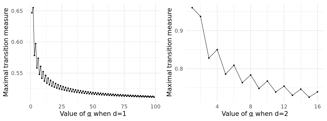
Refer to caption
Figure 6: Evaluation of LHS of equation (86) for $d=1,2$ and various regularity parameters.

B.6 Proof of Lemma 8

Proof.

For all $j\in\mathbb{N}$, write $E_{j}=G_{j}-P_{j}$. By Condition 2, for all $X_{i}\in\mathcal{N}_{j}$, $X_{i}$ and its parent set is included in a cube $\mathcal{C}$ with side length no greater than $c_{L}\gamma^{-j}$, which can be regarded as rescaling the unit cube $[0,1]^{d}$ with the rescaling parameter $c_{L}\gamma^{-j}$. Combining this with Lemma 6, we have

$$\|E_{j}\|_{\infty}\lesssim\gamma^{-2j(\alpha-\underline{\alpha})}+\gamma^{-j}.$$

The key idea of the proof is based on the fact that the operator $E_{j}$, the difference between Gaussian interpolation and polynomial interpolation, goes to zero exponentially fast as $j$ goes to infinity. It means $\|E_{j}\|_{\infty}$ not only converges to zero, but also sums up to a finite constant. This allows us to define certain partial sums that are Cauchy sequences, which will prove the lemma.

Let $\alpha^{*}=\min\{2(\alpha-\underline{\alpha}),1\}$ and note that $\|E_{j}\|_{\infty}\lesssim\gamma^{-\alpha^{*}j}$. For $j=j_{1}$, write

$$G_{j_{1}}=P_{j_{1}}+E_{j_{1}}=a_{j_{1}}P_{j_{1}}H_{j_{1}}+a_{j_{1}+1}H_{j_{1}+1}$$ (88)

with $a_{j_{1}}=1$, $a_{j_{1}+1}=\gamma^{-j_{1}\alpha^{*}}$, $H_{j_{1}}=I$(identity operator) and

$$\|H_{j_{1}+1}\|_{\infty}=\|E_{j_{1}}/\gamma^{-j_{1}\alpha^{*}}\|_{\infty}\lesssim 1.$$

We prove below that for all $j_{1}\leq j\leq j_{2}+1$, there exists an operator $\|H_{j+1}\|_{\infty}\lesssim 1$ and a constant $a_{j}\in[0,+\infty)$, such that

$$G_{j}\cdots G_{j_{1}+1}G_{j_{1}}=\sum_{j^{\prime}=j_{1}}^{j}a_{j^{\prime}}P_{j}\cdots P_{j^{\prime}+1}P_{j^{\prime}}H_{j^{\prime}}+a_{j+1}H_{j+1}.$$ (89)

Moreover, the constants $a_{j^{\prime}},j_{1}\leq j^{\prime}\leq j_{2}+1$ satisfy

$$a_{j+1}\lesssim\gamma^{-j\alpha^{*}}\sum_{j^{\prime}=j_{1}}^{j}a_{j^{\prime}}.$$

Then, let us introduce the notation $S_{j}=\sum_{j^{\prime}=j_{1}}^{j}a_{j^{\prime}}$, and note that by the preceding display

$$S_{j+1}-S_{j}\lesssim\gamma^{-j\alpha^{*}}S_{j}.$$

After reorganizing the inequality and using logarithmic transformation we arrive at

$\displaystyle\ln S_{j}\leq$ $\displaystyle\ln S_{j-1}(1+c\gamma^{-(j-1)\alpha^{*}})$
$\displaystyle\leq$ $\displaystyle\ln S_{j_{1}}+\sum_{j^{\prime}=0}^{j-1}\ln(1+c\gamma^{-j^{\prime}\alpha^{*}})\leq\ln a_{j_{1}}+c\sum_{j^{\prime}=0}^{\infty}\gamma^{-j^{\prime}\alpha^{*}}\leq\frac{c}{1-\gamma^{-\alpha^{*}}},$

for some universal constant $c>0$. Therefore, in view of Condition 3, we have

$$\|G_{j_{2}}\cdots G_{j_{1}+1}G_{j_{1}}\|_{\infty}\lesssim S_{j_{2}}\lesssim\exp\left[\frac{c}{1-\gamma^{-\alpha^{*}}}\right]\lesssim 1,$$

providing the claim of the lemma.

Hence it remained to prove (89). We proceed with proof by induction. By equation (88), the claim holds for $j=j_{1}$. Now suppose the claim holds for $j=l$. Then for $j=l+1$, we have

$\displaystyle G_{l+1}G_{l}\cdots G_{j_{1}+1}G_{j_{1}}=$ $\displaystyle(P_{l+1}+E_{l+1})\Big{[}\sum_{j^{\prime}=j_{1}}^{l}a_{j^{\prime}}P_{l}\cdots P_{j^{\prime}+1}P_{j^{\prime}}H_{j^{\prime}}+a_{l+1}H_{l+1}\Big{]}$
$\displaystyle=$ $\displaystyle\sum_{j^{\prime}=j_{1}}^{l+1}a_{j^{\prime}}P_{l+1}P_{l}\cdots P_{j^{\prime}+1}P_{j^{\prime}}H_{j^{\prime}}$
$\displaystyle\qquad+E_{l+1}\Big{[}\sum_{j^{\prime}=j_{1}}^{l}a_{j^{\prime}}P_{l}\cdots P_{j^{\prime}+1}P_{j^{\prime}}H_{j^{\prime}}+a_{l+1}H_{l+1}\Big{]}.$

Let $a_{l+2}=\|E_{l+1}\|\Big{\|}\sum_{j^{\prime}=j_{1}}^{l}a_{j^{\prime}}P_{l}\cdots P_{j^{\prime}+1}P_{j^{\prime}}H_{j^{\prime}}+a_{l+1}H_{l+1}\Big{\|}$ and

$$H_{l+2}=\Big{[}\sum_{j^{\prime}=j_{1}}^{l}a_{j^{\prime}}P_{l}\cdots P_{j^{\prime}+1}P_{j^{\prime}}H_{j^{\prime}}+a_{l+1}H_{l+1}\Big{]}/a_{l+2},$$

then obviously $\|H_{l+2}\|\leq 1$. Using Condition 3 and the induction assumption that $\|H_{j}\|_{1}\leq 1,\forall j_{1}\leq j\leq l+1$, we have

$$a_{l+2}\lesssim\|E_{l+1}\|\sum_{j=j_{1}}^{l+1}a_{j}\lesssim\gamma^{-(l+1)\alpha^{*}}\sum_{j=j_{1}}^{l+1}a_{j},$$

concluding the proof of the lemma. ∎

C Proofs of the lemmas and theorems in Section 4.3 and 4.4

C.1 Proof of Theorem 2

Proof.

We first prove the theorem with $s=1$ and abbreviate $\hat{Z}^{\tau,1}$ as $\hat{Z}^{\tau}$. Extending the result for general $s>0$ is straightforward and can be achieved by dividing $\epsilon$ by $s$.

Recall that $\eta(i)=j$ denotes that $X_{i}\in\mathcal{N}_{j}$. For all $X_{i}\in\mathcal{X}_{n}$, define $u_{i}$ as

$$u_{i}=\hat{Z}^{\tau}_{X_{i}}-\mathbb{E}(\hat{Z}^{\tau}_{X_{i}}|\hat{Z}^{\tau}_{\mathrm{pa}(X_{i})})=\hat{Z}^{\tau}_{X_{i}}-K_{\tau X_{i},\tau\mathrm{pa}(X_{i})}K_{\tau\mathrm{pa}(X_{i}),\tau\mathrm{pa}(X_{i})}^{-1}\hat{Z}^{\tau}_{\mathrm{pa}(X_{i})}.$$

Since $u_{i}$ is a linear transformation of a centered Gaussian random vector, it has also zero mean. Recall also that in view of Theorem 1, $\mathrm{Var}(u_{i})=\mathbb{E}[Z^{\tau}_{X_{i}}-\mathbb{E}(Z^{\tau}_{X_{i}}|Z^{\tau}_{\mathrm{pa}(X_{i})})]^{2}\asymp\tau^{2\alpha}\gamma^{-2\alpha\eta(i)}$. Furthermore, let $j_{0}$ be the smallest integer satisfying $\gamma^{-\alpha j_{0}}\leq\epsilon$ and define the sequence

$$b_{j}=\Bigg{\{}\begin{aligned} &\tau^{\alpha}\gamma^{-(\frac{j_{0}-j}{2}+j_{0})\alpha},&\;j<j_{0},\\ &\tau^{\alpha}\gamma^{-(\frac{j-j_{0}}{2}+j_{0})\alpha},&\;j\geq j_{0}.\end{aligned}$$

Finally, for all $1\leq i\leq n$, define the event $A_{i}=\{|u_{i}|\leq b_{\eta(i)}\}.$

The rest of the proof consists of three parts. In the first part, we will upper bound the $l_{\infty}$ norm of $\hat{Z}_{X_{i}}^{\tau}$ under the event $\cap_{i=1}^{n}A_{i}$. In the second part, we will derive a lower bound for the probability of this event $\cap_{i=1}^{n}A_{i}$. In the final part, we combine the previous results and extend them to general scaling parameter $s>0$.

Part 1: We restrict ourselves to the event $\cap_{i=1}^{n}A_{i}$. Then, for all $1\leq j\leq\eta(i)$, let us define the function $W_{j}:\cup_{j^{\prime}=0}^{j}\mathcal{N}_{j^{\prime}}\to\mathbb{R}$ as

$$W_{j}(X_{i})=\Bigg{\{}\begin{aligned} &u_{i},\;\;&X_{i}\in\mathcal{N}_{j},\\ &0,\;\;&X_{i}\not\in\mathcal{N}_{j}.\end{aligned}$$

With a slight abuse of notations, for all $1\leq j\leq\eta(n)$, let $\hat{Z}^{\tau}_{\cup_{j^{\prime}=0}^{j}\mathcal{N}_{j^{\prime}}}$ denote the restriction of $\hat{Z}^{\tau}$ to the co-domain $\cup_{j^{\prime}=0}^{j}\mathcal{N}_{j^{\prime}}$. Then recalling the definition of the operator $G_{j}$ in (31), we have for all $0\leq j\leq\eta(i)-1$,

$$\hat{Z}^{\tau}_{\cup_{j^{\prime}=0}^{j+1}\mathcal{N}_{j^{\prime}}}=W_{j+1}+G_{j}\hat{Z}^{\tau}_{\cup_{j^{\prime}=0}^{j}\mathcal{N}_{j^{\prime}}}.$$

Therefore, by induction of the previous formula, and in view of triangle inequality, the definition of the event $A_{i}$, and Lemma 8, we get

$\displaystyle\|\hat{Z}^{\tau}_{\mathcal{X}_{n}}\|_{\infty}=$ $\displaystyle\|\sum_{j=0}^{\eta(n)}G_{\eta(n)}G_{\eta(n)-1}\cdots G_{j+1}G_{j}W_{j}\|_{\infty}$
$\displaystyle\leq$ $\displaystyle\sum_{j=0}^{\eta(n)}\|G_{\eta(n)}G_{\eta(n)-1}\cdots G_{j+1}G_{j}W_{j}\|_{\infty}$
$\displaystyle\lesssim$ $\displaystyle\sum_{j^{\prime}=0}^{j}b_{j}\leq 2\tau^{\alpha}\frac{\gamma^{-\alpha j_{0}}}{1-\gamma^{-\alpha/2}}\lesssim\tau^{\alpha}\epsilon.$ (90)

Part 2: We first prove by induction that $u_{1},u_{2},\cdots,u_{n}$ are independent random variables. A single random variable $u_{1}$ is trivially independent. Then, assuming that $u_{1},u_{2},\cdots,u_{l}$ are independent we show below that $u_{l+1}$ is independent from $(u_{1},u_{2},\cdots,u_{l})$. By definition of $u_{i},1\leq i\leq l+1$, we have

$\displaystyle\mathbb{E}$ $\displaystyle\left\{u_{l+1}[u_{1},u_{2},\cdots,u_{l}]^{T}\right\}$
$\displaystyle\quad=\mathbb{E}\left\{\mathbb{E}\Big{\{}[\hat{Z}^{\tau}_{X_{l+1}}-\mathbb{E}(\hat{Z}^{\tau}_{X_{l+1}}|\hat{Z}^{\tau}_{\mathrm{pa}(X_{l+1})})][u_{1},u_{2},\cdots,u_{l}]^{T}\big{|}Z^{\tau}_{X_{i}},1\leq i\leq l\Big{\}}\right\}=0,$

which implies independence in view that $u_{i}$s are centered Gaussian random variables. Therefore,

$\displaystyle\mathrm{Pr}(\cap_{i=1}^{n}A_{i})=\prod_{i=1}^{n}\mathrm{Pr}\Big{(}|Z|\leq b_{\eta(i)}/\sqrt{\mathrm{Var}(u_{i})}\Big{)}=\prod_{j=1}^{\eta(n)}\left[\mathrm{Pr}(|Z|\leq b_{j}\tau^{-\alpha}\gamma^{\alpha j})\right]^{|\mathcal{N}_{j}|},$

where $Z\sim N(0,1)$. Then in view of the tail beahviour of the standard normal distribution

$\displaystyle\mathrm{Pr}(|Z|\leq u)$ $\displaystyle\geq u/3,\quad\forall\;0\leq u\leq 1,$
$\displaystyle\mathrm{Pr}(|Z|\leq u)$ $\displaystyle\geq 1-e^{-u^{2}}\geq\exp\big{(}-2e^{-u^{2}/2}\big{)},\quad\forall\;u\geq 1,$

see (7.2) and (7.3) in [34], respectively, the bound $b_{j}\tau^{-\alpha}\gamma^{\alpha j}\leq 1$ if and only if $j\leq j_{0}$ and noting that (44) implies $|\mathcal{N}_{j}|\lesssim\gamma^{dj}$, we get that for some constant $c_{d}>0$

$\displaystyle\mathrm{Pr}(\cap_{i=1}^{n}A_{i})\geq$ $\displaystyle\prod_{j=1}^{j_{0}}\big{(}\gamma^{-\frac{3}{2}\alpha(j_{0}-j)}/3\big{)}^{c_{d}\gamma^{dj}}\prod_{j=j_{0}+1}^{\eta(n)}\exp\big{(}-2c_{d}\gamma^{dj}e^{-\gamma^{\alpha(j-j_{0})}/2}\big{)}.$ (91)

The logarithm of the first term in (91) can be bounded as

$\displaystyle-\ln\prod_{j=1}^{j_{0}}\big{(}\gamma^{-\frac{3}{2}\alpha(j_{0}-j)}/3\big{)}^{c_{d}\gamma^{dj}}=$ $\displaystyle\sum_{j=1}^{j_{0}}c_{d}\gamma^{dj}\big{[}\frac{3}{2}\alpha(j_{0}-j)\ln\gamma+\ln 3]$
$\displaystyle=$ $\displaystyle c_{d}\gamma^{dj_{0}}\sum_{j=1}^{j_{0}}\gamma^{-d(j_{0}-j)}\big{[}\frac{3}{2}\alpha(j_{0}-j)\ln 2\gamma+\ln 3]\lesssim\gamma^{dj_{0}}.$

The logarithm of the second term in (91) can be bounded as

$\displaystyle-\ln\prod_{j=j_{0}+1}^{\eta(n)}\exp\big{(}-2c_{d}\gamma^{dj}e^{-\frac{1}{2}\gamma^{\alpha(j-j_{0})}}\big{)}=$ $\displaystyle\sum_{j=j_{0}+1}^{\eta(n)}2c_{d}\gamma^{dj}e^{-\frac{1}{2}\gamma^{\alpha(j-j_{0})}}\lesssim\gamma^{dj_{0}}.$

By combining the previous three displays and recalling that $\gamma^{-\alpha j_{0}}\asymp\epsilon$, we have get

$$-\ln\mathrm{Pr}(\cap_{i=1}^{n}A_{i})\lesssim\epsilon^{-d/\alpha}.$$ (92)

Conclusion: In view of asserttions (C.1) and (92), we have

$$-\ln\mathrm{Pr}\left(\|\hat{Z}^{\tau}_{\mathcal{X}_{n}}\|_{\infty}\lesssim\tau^{\alpha}\epsilon\right)\leq-\ln\mathrm{Pr}(\cap_{i=1}^{n}A_{i})\lesssim\epsilon^{-d/\alpha}.$$

This implies, replacing $\epsilon$ with $\epsilon\tau^{-\alpha}$, that

$$-\ln\mathrm{Pr}(\|\hat{Z}^{\tau}_{\mathcal{X}_{n}}\|_{\infty}\leq\epsilon)\lesssim\tau^{d}\epsilon^{-d/\alpha}.$$

Finally, noticing that $\hat{Z}^{\tau,s}=s\hat{Z}^{\tau}$, provides the statement of the theorem, i.e.

$$-\ln\mathrm{Pr}(\|\hat{Z}^{\tau,s}_{\mathcal{X}_{n}}\|_{\infty}<\epsilon)\lesssim\tau^{d}s^{d/\alpha}\epsilon^{-d/\alpha},$$

where the constant in $\lesssim$ depends only on $d,\alpha$. ∎

C.2 Proof of Lemma 9

Proof.

Let $f\in\mathbb{H}$ be an arbitrary function satisfying $\bm{f}(A)=\bm{f}_{0}(A)$. Then $f(x)-\sum_{i=1}^{|A|}a_{i}K(x_{i},x)=0$, $\forall x\in A$. By the definition of RKHS, we have

$$\langle K(x,\cdot),f(\cdot)-\sum_{i=1}^{|A|}a_{i}K(x_{i},\cdot)\rangle_{\mathbb{H}}=f(x)-\sum_{i=1}^{|A|}a_{i}K(x_{i},x)=0,\;\;\forall x\in A.$$

Therefore $K(x,\cdot)$ is orthogonal to $f(\cdot)-\sum_{i=1}^{|A|}a_{i}K(x_{i},\cdot)$ in $\mathbb{H}$, $\forall x\in A$. Thus

$\displaystyle\|f\|_{\mathbb{H}}^{2}$ $\displaystyle=\|f(\cdot)-\sum_{i=1}^{|A|}a_{i}K(x_{i},\cdot)\|_{\mathbb{H}}^{2}+\|\sum_{i=1}^{|A|}a_{i}K(x_{i},\cdot)\|_{\mathbb{H}}^{2}$
$\displaystyle\geq\|\sum_{i=1}^{|A|}a_{i}K(x_{i},\cdot)\|_{\mathbb{H}}^{2}=\bm{f}_{0}(A)^{T}K_{A,A}^{-1}\bm{f}_{0}(A).$

The minimal is achieved if and only if $f(\cdot)-\sum_{i=1}^{|A|}a_{i}K(x_{i},\cdot)=0$. ∎

C.3 Proof of Lemma 11

Proof.

In view of equation (2.2), without loss of generality, we can assume that $s=1$ and simplify the notation $Z^{\tau,1}$ as $Z^{\tau}$ and $\mathbb{H}^{\tau,1}$ as $\mathbb{H}^{\tau}$. The proof consists of three steps. In the first step, we control the interpolation error for constant functions. Then in the second step, we prove the lemma for $\beta\in(0,1]$. In the final step, we extend the proof for $\beta>1$.

Let us introduce the notation $B_{i}=\{X_{i}\}\cup\mathrm{pa}(X_{i})$. Then, in view of Condition 2, there exists a $d$-dimensional cube $\mathcal{C}\subset\mathcal{X}$ of length size $c_{L}\gamma^{-\eta(i)}$, which contains $B_{i}$. Also recall Condition 1, that the minimal $\ell^{\infty}$ distance among elements in $\cup_{j^{\prime}=0}^{j}\mathcal{N}_{j^{\prime}}$ is $c_{d}\gamma^{-j}$. Since the cube $\mathcal{C}$ contains $X_{i}$ and its parent set, we have $c_{d}\leq c_{L}$.

Step 1: Let $f_{0}\equiv c$ for some $c\in[-1,1]$. We prove that

$$\left|c-\mathbb{E}[Z^{\tau}_{X_{i}}|Z^{\tau}_{\mathrm{pa}(X_{i})}=c\mathbbm{1}]\right|\lesssim\gamma^{-\eta(i)\alpha},$$ (93)

where $\mathbbm{1}$ denotes the column vector of $1$s. Note, that in view of Lemma 9,

$$\inf_{f\in\mathbb{H}^{\tau},\bm{f}(B_{i})=\bm{f}_{0}(B_{i})}\|f\|_{\mathbb{H}^{\tau}}^{2}=\bm{f}_{0}(B_{i})^{T}K_{\tau B_{i},\tau B_{i}}^{-1}\bm{f}_{0}(B_{i})=\inf_{f\in\mathbb{H},\bm{f}(\tau B_{i})=\bm{f}_{0}(B_{i})}\|f\|_{\mathbb{H}}^{2}.$$ (94)

Then let us consider a function $\varphi_{0}(\cdot):\mathbb{R}\to\mathbb{R}$ such that $\varphi_{0}\in C^{\alpha+d/2}(\mathbb{R})_{1}$, $\varphi_{0}$ is supported on $[-2,2]$ and equals a constant on $[-1,1]$ and define the function $\varphi_{d}(\cdot):\mathbb{R}^{d}\to\mathbb{R}$ as $\varphi_{d}(x)=\prod_{l=1}^{d}\varphi_{0}(x[l])$. Noting that $\varphi_{d}\in C^{\alpha+d/2}(\mathbb{R}^{d})_{1}$ is supported on $[-2,2]^{d}$ and equals a constant on $[-1,1]^{d}$, $\varphi_{d}$ also has finite Sobolev norm, i.e., $\|f\|_{W^{\alpha+d/2}}\lesssim 1$. We then divide the proof into two cases based on whether $\tau\gamma^{-\eta(i)}\geq 1$.

If $\tau\gamma^{-\eta(i)}\leq 1$, consider the function

$$\tilde{f}(x)=\frac{c}{\varphi_{d}(0)}\varphi_{d}((x-\tau X_{i})/c_{L}).$$

Note that $\tilde{f}(x)=c$ for all $x\in\tau\mathcal{C}$. In view of the proof of Lemma 11.36 of [22], the RKHS norm is equivalent to the Sobolev norm. Therefore, by recalling (94),

$\displaystyle\inf_{f\in\mathbb{H}^{\tau},\,f(x)=c,\,x\in B_{i}}\|f\|_{\mathbb{H}^{\tau}}^{2}\leq$ $\displaystyle\|\tilde{f}\|_{\mathbb{H}}^{2}\asymp\|\tilde{f}\|_{W^{\alpha+d/2}}^{2}\asymp\|\varphi_{d}\|_{W^{\alpha+d/2}}^{2}\lesssim 1.$ (95)

If $\tau\gamma^{-\eta(i)}\geq 1$, then $\tau\geq 1$. Consider the function

$$\tilde{f}(x)=\sum_{w\in B_{i}}\tilde{f}_{w}(x),\qquad\text{with $\tilde{f}_{w}(x)=\frac{c}{\varphi_{d}(0)}\varphi_{d}\Big{(}\frac{4\sqrt{d}}{c_{d}}(x-w)\Big{)}$}.$$

Note, that $\tilde{f}_{w}(x)=c$ and $\tilde{f}_{w}(x)$ supported in a cube centered at $w$ with side length $c_{d}/(2\sqrt{d})$, which belongs to a ball centered at $w$ with radius $c_{d}/2\leq c_{d}\tau\gamma^{-\eta(i)}/2\leq c_{L}\tau\gamma^{-\eta(i)}/2$. Thus, the supports of the functions $\tilde{f}_{w}(x)$ are not overlapping. These imply $\tilde{f}(x)=c,\forall x\in\tau B_{i}$ and

$\displaystyle\inf_{f\in\mathbb{H}^{\tau},\,f(x)=c,\,x\in B_{i}}\|f\|_{\mathbb{H}^{\tau}}^{2}\leq$ $\displaystyle\|\tilde{f}\|_{\mathbb{H}}^{2}\asymp\|\tilde{f}\|_{W^{\alpha+d/2}}^{2}\lesssim(m+1)^{2}\|\varphi_{d}\|_{W^{\alpha+d/2}}^{2}\lesssim 1.$ (96)

Plugging in the bounds (95) and (96) into Lemma 10 and using Theorem 1, we get

$\displaystyle\left|c-\mathbb{E}[Z^{\tau}_{X_{i}}|Z^{\tau}_{\mathrm{pa}(X_{i})}=c\mathbbm{1}]\right|$ $\displaystyle\lesssim\sqrt{\mathrm{Var}\big{\{}Z^{\tau}_{X_{i}}-\mathbb{E}[{Z}^{\tau}_{X_{i}}|{Z}^{\tau}_{\mathrm{pa}(X_{i})}]\big{\}}\inf_{f\in\mathbb{H}^{\tau},\bm{f}(B_{i})=\bm{f}_{0}(B_{i})}\|f\|_{\mathbb{H}^{\tau}}^{2}}$
$\displaystyle\lesssim\sqrt{\tau^{2\alpha}\gamma^{-2\eta(i)\alpha}\cdot 1}=\tau^{\alpha}\gamma^{-\eta(i)\alpha}.$ (97)

Step 2: In view of $f_{0}\in C^{\beta}(\mathbb{R})_{1}$, $\beta\in(0,1]$, for all $w_{1},w_{2}\in[0,1]^{d}$,

$$\frac{|f_{0}(w_{1})-f_{0}(w_{2})|}{\|w_{1}-w_{2}\|_{2}^{\beta}}\leq 1.$$

Since for all $w_{1},w_{2}\in B_{i}$, $\|w_{1}-w_{2}\|\asymp\gamma^{-\eta(i)}$, for $c=f_{0}(X_{i})$ we have

$$|f_{0}(w)-c|\leq\|w-X_{i}\|_{2}^{\beta}\lesssim\gamma^{-\eta(i)\beta},\;\;\forall w\in B_{i}.$$ (98)

Denote $f_{c}(x)=f_{0}(x+X_{i})-c$, then $|f_{c}(x)|\lesssim\gamma^{-\eta(i)\beta}$, for all $x\in B_{i}-X_{i}$. Note, that assertion (94) holds with $f_{c}$ in place of $f_{0}$. We proceed next by splitting the proof based on the value of $\tau.$

If $\tau\gamma^{-\eta(i)}\leq 1$, let us consider the function

$$\tilde{f}(x)=\sum_{w\in B_{i}}\tilde{f}_{w}(x),\qquad\text{with\,\, $\tilde{f}_{w}(x)=\frac{f_{c}(w)}{\varphi_{d}(0)}\varphi_{d}\Big{(}\frac{x-\tau(w-X_{i})}{c_{d}\tau\gamma^{-\eta(i)}/4}\Big{)}$}.$$

Noting that the minimal separation distance among elements in $B_{i}$ is $c_{d}\gamma^{-\eta(i)}$ and $\forall w\in B_{i},\;\tilde{f}_{w}$ is supported on a cube with side length $c_{d}\tau\gamma^{-\eta(i)}/2$, the supports of $\tilde{f}_{w},w\in B_{i}$ are disjoint. Since $\tilde{f}_{w}(\tau(w-X_{i}))=f_{c}(w)$, denoting $\hat{\varphi}_{d}(\cdot)$ as the Fourier transform of $\varphi_{d}(\cdot)$, we have by equation (93),

$\displaystyle\inf_{f\in\mathbb{H}^{\tau},\bm{f}(B_{i})\leq\bm{f}_{c}(B_{i})}\|f\|_{\mathbb{H}^{\tau}}^{2}=$ $\displaystyle\|\tilde{f}\|_{\mathbb{H}}^{2}$
$\displaystyle\lesssim$ $\displaystyle\frac{\sum_{w\in B_{i}}[f_{c}(w)]^{2}}{[\varphi_{d}(0)]^{2}}\int\big{|}(\tau\gamma^{-\eta(i)})^{d}\hat{\varphi}_{d}(\lambda c_{d}\tau\gamma^{-\eta(i)})\big{|}^{2}(1+\|\lambda\|^{2})^{\alpha+d/2}d\lambda$
$\displaystyle\lesssim$ $\displaystyle\gamma^{-2\eta(i)\beta}\tau^{d}\gamma^{-\eta(i)d}\int\big{|}\hat{\varphi}_{d}(\lambda c_{d}\tau\gamma^{-\eta(i)})\big{|}^{2}(1+\|\lambda\|^{2})^{\alpha+d/2}d(\tau\gamma^{-\eta(i)}\lambda)$
$\displaystyle\lesssim$ $\displaystyle\gamma^{-2\eta(i)\beta}\tau^{d}\gamma^{-\eta(i)d}\sup_{\lambda}\frac{(1+\|\lambda\|^{2})^{\alpha+d/2}}{(1+\|\lambda c_{d}\tau\gamma^{-\eta(i)}\|^{2})^{\alpha+d/2}}\|\varphi_{d}\|^{2}_{W_{2,\alpha+d/2}}$
$\displaystyle\lesssim$ $\displaystyle\gamma^{-2\eta(i)\beta}\tau^{d}\gamma^{-\eta(i)d}(\tau\gamma^{-\eta(i)})^{-(2\alpha+d)}$
$\displaystyle=$ $\displaystyle\tau^{-2\alpha}\gamma^{2\eta(i)(\alpha-\beta)}.$ (99)

If $\tau\gamma^{-\eta(i)}\geq 1$, let us take

$$\tilde{f}(x)=\sum_{w\in B_{i}}\frac{f_{c}(w)}{\varphi_{d}(0)}\varphi_{d}\Big{(}\frac{4\sqrt{d}}{c_{d}}(x-w)\Big{)}.$$

By the same analysis as in Step 1, we have

$\displaystyle\inf_{f\in\mathbb{H}^{\tau},\bm{f}(B_{i})=\bm{f}_{c}(B_{i})}\|f\|_{\mathbb{H}^{\tau}}^{2}\lesssim\sum_{w\in B_{i}}[f_{c}(w)]^{2}\|\varphi_{d}\|^{2}_{W^{\alpha+d/2}}\asymp\sum_{w\in B_{i}}[f_{c}(w)]^{2}\lesssim\gamma^{-2\eta(i)\beta},$ (100)

where the last step follows from (98). Plugging in the bounds (C.3) and (100) into Lemma 10,

$\displaystyle\left|f_{c}(X_{i})-\mathbb{E}[Z^{\tau}_{X_{i}}|Z^{\tau}_{\mathrm{pa}(X_{i})}=\bm{f}_{c}(\mathrm{pa}(X_{i}))]\right|\lesssim$ $\displaystyle\sqrt{\tau^{2\alpha}\gamma^{-2\eta(i)\alpha}\cdot[\tau^{-2\alpha}\gamma^{2\eta(i)(\alpha-\beta)}+\gamma^{-2\eta(i)\beta}]}$
$\displaystyle\lesssim$ $\displaystyle\gamma^{-\eta(i)\beta}+\tau^{\alpha}\gamma^{-\eta(i)(\alpha+\beta)}.$ (101)

Then in view of (C.3) and (93), the linearity of the expectation, and $\gamma^{\eta(i)\beta}\geq 1$,

$\displaystyle\left|f_{0}(X_{i})-\mathbb{E}[Z^{\tau}_{X_{i}}|Z^{\tau}_{\mathrm{pa}(X_{i})}=\bm{f}_{0}(\mathrm{pa}(X_{i}))]\right|$ $\displaystyle\lesssim\tau^{\alpha}\gamma^{-\eta(i)\alpha}+\gamma^{-\eta(i)\beta}+\tau^{\alpha}\gamma^{-\eta(i)(\alpha+\beta)}$
$\displaystyle\lesssim\tau^{\alpha}\gamma^{-\eta(i)\alpha}+\gamma^{-\eta(i)\beta},$

proving the lemma for $\beta\in(0,1]$.

Step 3: Finally, we extend the proof for $\beta>1$. We use proof by induction on $\beta$. The case when $\beta\in(0,1]$ is proved in Step 2. Suppose the lemma holds for $\beta\in(0,r]$ for some $r\in\mathbb{N}_{+}$. Now consider the case when $\beta\in(r,r+1]$. Because $r\geq 1$, $f_{0}$ is a differentiable function. For arbitrary choice of $\zeta=(\zeta[1],\zeta[2],\cdots,\zeta[d])^{T}\in\mathcal{C}$,

$$f_{0}(x)=f_{0}(\zeta)+\sum_{l=1}^{d}\int_{\zeta[l]}^{x[l]}\frac{\partial}{\partial t}f_{0}(\zeta[1],\ldots,\zeta[l-1],t,x[l+1],\ldots,x[d])dt.$$

Define the operator $\mathcal{L}$ such that $\forall f:\mathcal{X}\to\mathbb{R},\;x\in\mathcal{X}$ , $\mathcal{L}(f)(x)=f(x)-\mathbb{E}[Z^{\tau}_{x}|Z^{\tau}_{\mathrm{pa}(X_{i})}=\bm{f}(\mathrm{pa}(X_{i}))]$. Note that $\mathcal{L}$ is a linear operator and can exchange orders with summation and integration (as long as integration is finite). Then, in view of the induction assumption and the inequality (97), for all $x\in\mathcal{C}$

$\displaystyle\left|f_{0}(x)-\mathbb{E}[Z^{\tau}_{x}|Z^{\tau}_{\mathrm{pa}(X_{i})}=\bm{f}_{0}(\mathrm{pa}(X_{i}))]\right|$
$\displaystyle\leq$ $\displaystyle|\mathcal{L}(f_{0})(\zeta)|+\sum_{l=1}^{d}\int_{\zeta[l]}^{x[l]}\mathcal{L}\Big{(}\frac{\partial}{\partial t}f_{0}(\zeta[1],\ldots,\zeta[l-1],t,x[l+1],\ldots,x[d])\Big{)}dt$
$\displaystyle\lesssim$ $\displaystyle\tau^{\alpha}\gamma^{-\eta(i)\alpha}+d\gamma^{-\eta(i)}\big{[}\tau^{\alpha}\gamma^{-\eta(i)\alpha}+\gamma^{-\eta(i)(\beta-1)}\big{]}$
$\displaystyle\lesssim$ $\displaystyle\tau^{\alpha}\gamma^{-\eta(i)\alpha}+\gamma^{-\eta(i)\beta}.$

We conclude the proof by taking $x=X_{i}$. ∎

C.4 Proof of Lemma 12

Proof of Lemma 12.

The proof consists of three steps. In the first step, we derive a summation formula regarding the RKHS norms of $l(l\leq n)$-dimensional marginals of the process $\hat{Z}^{\tau,s}$. In the second step, we derive a decomposition for all functions in $\ell^{1}(\mathcal{X}_{n})$ using the difference formula in Lemma 11. Finally, we combine the previous two steps to finish the proof.

Step 1 Recall the formula for the RKHS of $\hat{Z}^{\tau,s}$ on $\mathcal{X}_{n}$, see (35). For all $l\leq n$, letting $\mathcal{X}_{l}=\{X_{1},X_{2},\cdots,X_{l}\}$, we prove that

$$\bm{f}_{0}(\mathcal{X}_{l})^{T}(\hat{K}^{\tau,s}_{\mathcal{X}_{l},\mathcal{X}_{l}})^{-1}\bm{f}_{0}(\mathcal{X}_{l})=\sum_{i=1}^{l}\frac{\big{\{}f_{0}(X_{i})-\mathbb{E}[{Z}^{\tau,s}_{X_{i}}|{Z}^{\tau,s}_{\mathrm{pa}(X_{i})}=\bm{f}_{0}(\mathrm{pa}(X_{i}))]\big{\}}^{2}}{\mathrm{Var}\big{\{}Z^{\tau,s}_{X_{i}}-\mathbb{E}[{Z}^{\tau,s}_{X_{i}}|{Z}^{\tau,s}_{\mathrm{pa}(X_{i})}]\big{\}}}.$$ (102)

For $i=1$, note that $X_{1}$ has no parents, implying (102) directly. Next, we assume that equation (102) holds for $l=1,2,\cdots,l^{\prime}$ and we show below that it holds also for $l=l^{\prime}+1$. Define the matrix $U\in\mathbb{R}^{(l^{\prime}+1)\times(l^{\prime}+1)}$ as

$$U=\begin{bmatrix}I&0\\ -(\hat{K}^{\tau,s}_{\mathcal{X}_{l^{\prime}},X_{{l^{\prime}}+1}})^{T}(\hat{K}^{\tau,s}_{\mathcal{X}_{l^{\prime}},\mathcal{X}_{l^{\prime}}})^{-1}&1\end{bmatrix},$$

and note that

$\displaystyle U\hat{K}^{\tau,s}_{\mathcal{X}_{l^{\prime}+1},\mathcal{X}_{l^{\prime}+1}}U^{T}=$ $\displaystyle\begin{bmatrix}\hat{K}^{\tau,s}_{\mathcal{X}_{l^{\prime}},\mathcal{X}_{l^{\prime}}}&0\\ 0&\hat{K}^{\tau,s}_{X_{l^{\prime}+1},X_{l^{\prime}+1}}-(\hat{K}^{\tau,s}_{\mathcal{X}_{l^{\prime}},X_{l^{\prime}+1}})^{T}(\hat{K}^{\tau,s}_{\mathcal{X}_{l^{\prime}},\mathcal{X}_{l^{\prime}}})^{-1}\hat{K}^{\tau,s}_{\mathcal{X}_{l^{\prime}},X_{l^{\prime}+1}}\end{bmatrix}.$

Taking the inverse of the above formula, and noting that $\hat{K}^{\tau,s}_{X_{l^{\prime}+1},X_{l^{\prime}+1}}=s^{2}$, the precision matrix on $\mathcal{X}_{l^{\prime}+1}$ can be computed as

$\displaystyle(\hat{K}^{\tau,s}_{\mathcal{X}_{l^{\prime}+1},\mathcal{X}_{l^{\prime}+1}})^{-1}$ $\displaystyle=U^{T}\begin{bmatrix}(\hat{K}^{\tau,s}_{\mathcal{X}_{l^{\prime}},\mathcal{X}_{l^{\prime}}})^{-1}&0\\ 0&\big{[}s^{2}-(\hat{K}^{\tau,s}_{\mathcal{X}_{l^{\prime}},X_{l^{\prime}+1}})^{T}(\hat{K}^{\tau,s}_{\mathcal{X}_{l^{\prime}},\mathcal{X}_{l^{\prime}}})^{-1}\hat{K}^{\tau,s}_{\mathcal{X}_{l^{\prime}},X_{{l^{\prime}}+1}})\big{]}^{-1}\end{bmatrix}U.$ (103)

For the conditional expectation, using the DAG structure of the Vecchia approximation and equation (2.2),

$\displaystyle(\hat{K}^{\tau,s}_{\mathcal{X}_{l^{\prime}},X_{l^{\prime}+1}})^{T}(\hat{K}^{\tau,s}_{\mathcal{X}_{l^{\prime}},\mathcal{X}_{l^{\prime}}})^{-1}\bm{f}_{0}(\mathcal{X}_{l^{\prime}})=$ $\displaystyle\mathbb{E}\big{[}\hat{Z}^{\tau,s}_{X_{l^{\prime}+1}}|\hat{Z}^{\tau,s}_{\mathcal{X}_{l^{\prime}}}=\bm{f}_{0}(\mathcal{X}_{l^{\prime}})\big{]}$
$\displaystyle=$ $\displaystyle\mathbb{E}\big{[}{Z}^{\tau,s}_{X_{l^{\prime}+1}}|{Z}^{\tau,s}_{\mathrm{pa}(X_{l^{\prime}+1})}=\bm{f}_{0}(\mathrm{pa}(X_{l^{\prime}+1}))\big{]}.$

The variance, can be rewritten along the same lines

$\displaystyle s^{2}-(\hat{K}^{\tau,s}_{\mathcal{X}_{l^{\prime}},X_{l^{\prime}+1}})^{T}(\hat{K}^{\tau,s}_{\mathcal{X}_{l^{\prime}},\mathcal{X}_{l^{\prime}}})^{-1}\hat{K}^{\tau,s}_{\mathcal{X}_{l^{\prime}},X_{{l^{\prime}}+1}}=$ $\displaystyle\mathrm{Var}\big{[}\hat{Z}^{\tau,s}_{X_{l^{\prime}+1}}-\mathbb{E}\big{[}\hat{Z}^{\tau,s}_{X_{l^{\prime}+1}}|\hat{Z}^{\tau,s}_{\mathcal{X}_{l^{\prime}}}\big{]}\big{]}$
$\displaystyle=$ $\displaystyle\mathrm{Var}\big{[}Z^{\tau,s}_{X_{l^{\prime}+1}}-\mathbb{E}\big{[}{Z}^{\tau,s}_{X_{l^{\prime}+1}}|{Z}^{\tau,s}_{\mathrm{pa}(X_{l^{\prime}+1})}\big{]}\big{]}.$ (104)

By combining the preceding displays and applying the induction assumption,

$\displaystyle\bm{f}_{0}(\mathcal{X}_{l^{\prime}+1})^{T}(\hat{K}^{\tau,s}_{\mathcal{X}_{l^{\prime}+1},\mathcal{X}_{l^{\prime}+1}})^{-1}\bm{f}_{0}(\mathcal{X}_{l^{\prime}+1})$
$\displaystyle=$ $\displaystyle\Big{[}U\bm{f}_{0}(\mathcal{X}_{l^{\prime}+1})\Big{]}^{T}\begin{bmatrix}(\hat{K}^{\tau,s}_{\mathcal{X}_{l^{\prime}},\mathcal{X}_{l^{\prime}}})^{-1}&0\\ 0&\big{[}s^{2}-(\hat{K}^{\tau,s}_{\mathcal{X}_{l^{\prime}},X_{l^{\prime}+1}})^{T}(\hat{K}^{\tau,s}_{\mathcal{X}_{l^{\prime}},\mathcal{X}_{l^{\prime}}})^{-1}\hat{K}^{\tau,s}_{\mathcal{X}_{l^{\prime}},X_{{l^{\prime}}+1}})\big{]}^{-1}\end{bmatrix}U\bm{f}_{0}(\mathcal{X}_{l^{\prime}+1})$
$\displaystyle=$ $\displaystyle\frac{\big{\{}f_{0}(X_{{l^{\prime}}+1})-\mathbb{E}[{Z}^{\tau,s}_{X_{{l^{\prime}}+1}}|{Z}^{\tau,s}_{\mathrm{pa}(X_{{l^{\prime}}+1})}=\bm{f}_{0}(\mathrm{pa}(X_{{l^{\prime}}+1}))]\big{\}}^{2}}{\mathrm{Var}\big{\{}Z^{\tau,s}_{X_{{l^{\prime}}+1}}-\mathbb{E}[{Z}^{\tau,s}_{X_{{l^{\prime}}+1}}|{Z}^{\tau,s}_{\mathrm{pa}(X_{{l^{\prime}}+1})}]\big{\}}}+\bm{f}_{0}(\mathcal{X}_{l^{\prime}})^{T}(K^{\tau,s}_{\mathcal{X}_{l^{\prime}},\mathcal{X}_{l^{\prime}}})^{-1}\bm{f}_{0}(\mathcal{X}_{l^{\prime}})$
$\displaystyle=$ $\displaystyle\sum_{i=1}^{{l^{\prime}}+1}\frac{\big{\{}f_{0}(X_{i})-\mathbb{E}[{Z}^{\tau,s}_{X_{i}}|{Z}^{\tau,s}_{\mathrm{pa}(X_{i})}=\bm{f}_{0}(\mathrm{pa}(X_{i}))]\big{\}}^{2}}{\mathrm{Var}\big{\{}Z^{\tau,s}_{X_{i}}-\mathbb{E}[{Z}^{\tau,s}_{X_{i}}|{Z}^{\tau,s}_{\mathrm{pa}(X_{i})}]\big{\}}}.$

Step 2 For all $0\leq j\leq\eta(n)$, we define the operator $\Theta_{j}:\ell^{1}(\mathcal{X}_{n})\to\ell^{1}(\cup_{j^{\prime}=0}^{j}\mathcal{N}_{j^{\prime}})$, such that for all $f\in\ell^{1}(\mathcal{X}_{n})$,

$$\Theta_{j}(f)(X_{i})=\Bigg{\{}\begin{aligned} &f(X_{i})-\mathbb{E}[{Z}^{\tau,s}_{X_{i}}|{Z}^{\tau,s}_{\mathrm{pa}(X_{i})}=\bm{f}(\mathrm{pa}(X_{i}))],&&X_{i}\in\mathcal{N}_{j},\\ &0,&&X_{i}\in\cup_{j^{\prime}=0}^{j-1}\mathcal{N}_{j^{\prime}}.\end{aligned}$$

The operator $\Theta_{j}$ “extracts” the differences between the function values on $\mathcal{N}_{j}$ and the conditional expectations on $\mathcal{N}_{j}$ based on the DAG structures. Our objective is to prove the following equation

$$f=\sum_{j=0}^{\eta(n)}G_{\eta(n)-1}\cdots G_{j+1}G_{j}\Theta_{j}(f).$$ (105)

Directly deriving equation (105) may not be very intuitive. Instead, we will prove by induction that for all $0\leq j\leq\eta(n)$,

$$f|_{\cup_{j^{\prime}=0}^{j}\mathcal{N}_{j^{\prime}}}=\sum_{j^{\prime}=0}^{j}G_{j-1}\cdots G_{j^{\prime}+1}G_{j^{\prime}}\Theta_{j^{\prime}}(f),$$ (106)

where $f|_{\cup_{j^{\prime}=0}^{j}\mathcal{N}_{j^{\prime}}}$ denotes the restriction of the function $f$ on the set $\cup_{j^{\prime}=0}^{j}\mathcal{N}_{j^{\prime}}$. For $j=0$, the domain $\cup_{j^{\prime}=0}^{j}\mathcal{N}_{j^{\prime}}$ is just $\mathcal{N}_{0}=\{X_{1}\}$ and

$$f(X_{1})=\Theta_{0}(f)(X_{1})=f(X_{1})-0=f(X_{1}).$$

Now suppose equation (106) holds for $j=\tilde{j}$. Consider the case that $j=\tilde{j}+1$. For all $X_{i}\in\cup_{j^{\prime}=0}^{\tilde{j}+1}\mathcal{N}_{j^{\prime}}$, we have

$\displaystyle f(X_{i})=$ $\displaystyle\Theta_{\tilde{j}+1}(f)(X_{i})+\mathbb{E}[{Z}^{\tau,s}_{X_{i}}|{Z}^{\tau,s}_{\mathrm{pa}(X_{i})}=\bm{f}(\mathrm{pa}(X_{i}))]$
$\displaystyle=$ $\displaystyle\Theta_{\tilde{j}+1}(f)(X_{i})+G_{\tilde{j}}(f|_{\cup_{j^{\prime}=0}^{\tilde{j}}\mathcal{N}_{j^{\prime}}})(X_{i}).$

Since this holds for all $X_{i}\in\cup_{j^{\prime}=0}^{\tilde{j}+1}\mathcal{N}_{j^{\prime}}$, applying equation (106) for $j=\tilde{j}$, we have

$\displaystyle f|_{\cup_{j^{\prime}=0}^{\tilde{j}+1}\mathcal{N}_{j^{\prime}}}=$ $\displaystyle\Theta_{\tilde{j}+1}(f)+G_{\tilde{j}}\sum_{j^{\prime}=0}^{\tilde{j}}G_{\tilde{j}-1}\cdots G_{j^{\prime}+1}G_{j^{\prime}}\Theta_{j^{\prime}}(f)=\sum_{j^{\prime}=0}^{\tilde{j}+1}G_{\tilde{j}}\cdots G_{j^{\prime}+1}\Theta_{j^{\prime}}(f),$

concluding the proof of (106) and hence also of (105).

Step 3 By Theorem 1 and Lemma 11,

$$\mathrm{Var}\big{\{}Z^{\tau,s}_{X_{i}}-\mathbb{E}[{Z}^{\tau,s}_{X_{i}}|{Z}^{\tau,s}_{\mathrm{pa}(X_{i})}]\big{\}}\asymp\tau^{2\alpha}s^{2}\gamma^{-2\alpha\eta(i)},$$
$$\big{|}f_{0}(X_{i})-\mathbb{E}[{Z}^{\tau,s}_{X_{i}}|{Z}^{\tau,s}_{\mathrm{pa}(X_{i})}=\bm{f}_{0}(\mathrm{pa}(X_{i}))]\big{|}\lesssim\tau^{\alpha}\gamma^{-\alpha\eta(i)}+\gamma^{-\beta\eta(i)}.$$

The above displays and equation (102) together with $l\leq\gamma^{\eta(l)d}$ imply,

$\displaystyle\bm{f}_{0}(\mathcal{X}_{l})^{T}(\hat{K}^{\tau,s}_{\mathcal{X}_{l},\mathcal{X}_{l}})^{-1}\bm{f}_{0}(\mathcal{X}_{l})$ $\displaystyle\lesssim\sum_{i=1}^{l}\frac{\tau^{2\alpha}\gamma^{-2\alpha\eta(i)}+\gamma^{-2\beta\eta(i)}}{\tau^{2\alpha}s^{2}\gamma^{-2\alpha\eta(i)}}$
$\displaystyle\leq s^{-2}\gamma^{\eta(l)d}+\tau^{-2\alpha}s^{-2}\gamma^{(2\alpha-2\beta+d)\eta(l)}.$

Let $f_{1}\in\mathbb{H}_{n}^{\tau,s}$ be the function satisfying $f_{1}(x)=f_{0}(x),\forall x\in\mathcal{X}_{l}$ and $\Theta_{j}(f_{1})=0,\forall\eta(l)\leq j\leq\eta(n)-1$. In view of equation (105) and Lemma 8,

$\displaystyle\sup_{1\leq i\leq n}|f_{0}(X_{i})-f_{1}(X_{i})|=$ $\displaystyle\Big{\|}\sum_{j=0}^{\eta(n)}G_{\eta(n)-1}\cdots G_{j+1}G_{j}\Theta_{j}(f_{1})-\sum_{j=0}^{\eta(n)}G_{\eta(n)-1}\cdots G_{j+1}G_{j}\Theta_{j}(f_{0})\Big{\|}_{\infty}$
$\displaystyle=$ $\displaystyle\bigg{\|}\sum_{j=\eta(l)}^{\eta(n)-1}G_{\eta(n)-1}\cdots G_{j+2}G_{j+1}\Big{[}\Theta_{j}(f_{1})-\Theta_{j}(f_{0})\Big{]}\bigg{\|}_{\infty}$
$\displaystyle\leq$ $\displaystyle\sum_{j=\eta(l)}^{\eta(n)-1}\|G_{\eta(n)-1}\cdots G_{j+2}G_{j+1}\|\cdot\big{(}\|\Theta_{j}(f_{1})\|_{\infty}+\|\Theta_{j}(f_{0})\|_{\infty}\big{)}$
$\displaystyle\lesssim$ $\displaystyle\sum_{j=\eta(l)}^{\eta(n)-1}(\tau^{\alpha}\gamma^{-j\alpha}+\gamma^{-j\beta})\lesssim\tau^{\alpha}\gamma^{-\eta(l)\alpha}+\gamma^{-\eta(l)\beta}.$

Let us denote by $c$ the constant multiplier in the upper bound $\lesssim$. Then, by choosing $l$ to be the smallest integer satisfying $c(\tau^{\alpha}\gamma^{-\eta(l)\alpha}+\gamma^{-\eta(l)\beta})\leq\epsilon_{n}$, we get

$$\|f_{1}-f_{0}\|_{\infty,n}\leq\epsilon_{n}.$$

If $\tau^{\alpha}\gamma^{-\eta(l)\alpha}\geq\gamma^{-\eta(l)\beta}$, then $\epsilon_{n}\asymp\tau^{\alpha}\gamma^{-\eta(l)\alpha}$, which in turn implies

$$\inf_{f\in\mathbb{H}_{n}^{\tau,s}:\|f-f_{0}\|_{\infty,n}\leq\epsilon_{n}}\|f\|_{\mathbb{H}_{n}^{\tau,s}}^{2}\leq\|f_{1}\|_{\mathbb{H}_{n}^{\tau,s}}^{2}\lesssim s^{-2}\gamma^{\eta(l)d}\asymp s^{-2}\tau^{d}\epsilon_{n}^{-d/\alpha}.$$

Otherwise, for $\tau^{\alpha}\gamma^{-\eta(l)\alpha}<\gamma^{-\eta(l)\beta}$, $\epsilon_{n}\asymp\gamma^{-\eta(l)\beta}$, hence

$$\inf_{f\in\mathbb{H}_{n}^{\tau,s}:\|f-f_{0}\|_{\infty,n}\leq\epsilon_{n}}\|f\|_{\mathbb{H}_{n}^{\tau,s}}^{2}\leq\|f_{1}\|_{\mathbb{H}_{n}^{\tau,s}}^{2}\lesssim s^{-2}\epsilon_{n}^{-d/\beta}+\tau^{-2\alpha}s^{-2}\epsilon_{n}^{-\frac{2(\alpha-\beta)+d}{\beta}}.$$

Combining these two cases results in the stated upper bound.

D Proofs of the theorems and corollaries in Section 5

D.1 Proof of Corollary 1

Proof.

The case that both $\tau$ and $s$ are constants can be directly obtained from Theorem 3. For the case that $\tau^{\alpha}s\asymp n^{\frac{\alpha-\beta}{2\beta+d}}$, plugging in the value of $\tau^{\alpha}s$ into equation (38), we have

$$n^{-\frac{\beta}{2\alpha+d}}(\tau^{\alpha}s)^{-\frac{2\beta}{2\alpha+d}}=n^{-\frac{\alpha}{2\alpha+d}}(\tau^{\alpha}s)^{\frac{d}{2\alpha+d}}=n^{-\frac{\beta}{2\beta+d}}.$$

Because $s\gtrsim 1$, we have

$$(ns^{2})^{-\frac{\beta}{2\beta+d}}\lesssim n^{-\frac{\beta}{2\beta+d}}\text{ and }(ns^{2}\tau^{-d})^{-\frac{\alpha}{2\alpha+d}}\lesssim n^{-\frac{\alpha}{2\alpha+d}}(\tau^{\alpha}s)^{\frac{d}{2\alpha+d}}.$$

Therefore the posterior contraction rate is $n^{-\frac{\beta}{2\beta+d}}$. ∎

D.2 Proof of Theorem 4

We first prove a (nearly) nested property of the RKHS balls corresponding to Vecchia GPs $\hat{Z}^{\tau,s}$ in view of the scaling parameters $s$ and $\tau$. For the space scaling parameter $s$ the inclusions are strictly monotone and straightforward. However, for the time rescaling $\tau$ it is substantially more challenging. To begin with, let us denote the unit balls in the RKHS and the Banach space $(\mathcal{X}_{n},\|\cdot\|_{n,\infty})$ by

$$\mathbb{H}_{n}^{\tau,s}(1)=\{f\in\mathbb{H}_{n}^{\tau,s}:\|f\|_{\mathbb{H}_{n}^{\tau,s}}\leq 1\},\quad\mathbb{B}_{n}(1)=\{f:\mathcal{X}_{n}\rightarrow\mathbb{R},\,\|f\|_{n,\infty}\leq 1\},$$

respectively.

Lemma 15.

There exists a universal constant $C>0$, such that for all $0<\tau,\Delta\tau,s,\Delta s$ with $\Delta\tau<1$, $0<\tau-\Delta\tau\leq\tau$ and $0<s-\Delta s\leq s$,

$$\mathbb{H}^{\tau,s}_{n}(1)\subset\mathbb{H}_{n}^{\tau-\Delta\tau,s-\Delta s}(C)+\mathbb{B}_{n}\big{(}C[\Delta\tau+\Delta\tau^{2(\alpha-\underline{\alpha})}]\tau^{\alpha}s\ln n\big{)}.$$
Proof.

The proof consists of two parts. First, we compare $\mathbb{H}_{n}^{\tau-\Delta\tau,s}(1)$ and $\mathbb{H}_{n}^{\tau,s}$ and then $\mathbb{H}_{n}^{\tau-\Delta\tau,s-\Delta s}$ and $\mathbb{H}_{n}^{\tau-\Delta\tau,s}$.

Step 1: For $f\in\mathbb{H}^{\tau,s}_{n}(1)$, in view of the definition of operator $\Theta_{j}$ and equations (33) and (102),

$$\|f\|_{\mathbb{H}^{\tau,s}_{n}}^{2}=\sum_{i=1}^{n}\frac{\big{\{}f(X_{i})-\mathbb{E}[{Z}^{\tau,s}_{X_{i}}|{Z}^{\tau,s}_{\mathrm{pa}(X_{i})}=\bm{f}(\mathrm{pa}(X_{i}))]\big{\}}^{2}}{\mathrm{Var}\big{\{}Z^{\tau,s}_{X_{i}}-\mathbb{E}[{Z}^{\tau,s}_{X_{i}}|{Z}^{\tau,s}_{\mathrm{pa}(X_{i})}]\big{\}}}=\sum_{i=1}^{n}\frac{[\Theta_{\eta(i)}(f)(X_{i})]^{2}}{\mathrm{Var}\big{\{}Z^{\tau,s}_{X_{i}}-\mathbb{E}[{Z}^{\tau,s}_{X_{i}}|{Z}^{\tau,s}_{\mathrm{pa}(X_{i})}]\big{\}}}.$$ (107)

Furthermore, recall the Gaussian interpolation operator $G_{j}:\cup_{j^{\prime}=0}^{j-1}\mathcal{N}_{j^{\prime}}\to\mathcal{N}_{j}$ in (31). We explicitly write out the rescaling parameter associated with the interpolating process $\hat{Z}^{\tau,s}$ and denote the operator as $G^{\tau}$. Similarly, for $\tilde{\tau}=\tau-\Delta\tau$, the operator $G^{\tilde{\tau}}$ means performing GP interpolation with respect to the process $\hat{Z}^{\tilde{\tau},s}$. In view of equation (105),

$$f=\sum_{j=0}^{\eta(n)}G^{\tau}_{\eta(n)-1}\cdots G^{\tau}_{j+1}G^{\tau}_{j}\Theta_{j}(f).$$

For $\tilde{\tau}=\tau-\Delta\tau$, we also define function $\tilde{f}$ on $\mathcal{X}$ as

$$\tilde{f}=\sum_{j=0}^{\eta(n)}G^{\tilde{\tau}}_{\eta(n)-1}\cdots G^{\tilde{\tau}}_{j+1}G^{\tilde{\tau}}_{j}\Theta_{j}(f).$$

By Lemma 8, there exists a constant $C$, such that for all $j_{1},j_{2}\in\mathbb{N}$,

$$\|\prod_{j=j_{1}}^{j_{2}}G^{\tau}_{j}\|\leq C,\;\;\|\prod_{j=j_{1}}^{j_{2}}G^{\tilde{\tau}}_{j}\|\leq C.$$ (108)

Since $0<\Delta\tau<1$, by Lemma 6, for all $j\in\mathbb{N}$,

$$\|G_{j}^{\tau}-G_{j}^{\tilde{\tau}}\|_{\infty}\lesssim\Delta\tau+\Delta\tau^{2(\alpha-\underline{\alpha})}.$$ (109)

Combing the previous two displays, i.e. (108) and (109), with the formulas for $f(\mathcal{X}_{n})$ and $\tilde{f}(\mathcal{X}_{n})$, we have

$\displaystyle\|f(\mathcal{X}_{n})-\tilde{f}(\mathcal{X}_{n})\|_{\infty}$ $\displaystyle=\Big{\|}\sum_{j=0}^{\eta(n)-1}(G^{\tau}_{\eta(n)-1}\cdots G^{\tau}_{j+1}G^{\tau}_{j}-G^{\tilde{\tau}}_{\eta(n)-1}\cdots G^{\tilde{\tau}}_{j+1}G^{\tilde{\tau}}_{j})\Theta_{j}(f)\Big{\|}_{\infty}$
$\displaystyle=\Big{\|}\sum_{j=0}^{\eta(n)-1}\sum_{l=j}^{\eta(n)-1}G_{\eta(n)-1}^{\tilde{\tau}}\cdots G_{l+1}^{\tilde{\tau}}(G_{l}^{\tau}-G_{l}^{\tilde{\tau}})G_{l-1}^{\tau}\cdots G_{j}^{\tau}\Theta_{j}(f)\Big{\|}_{\infty}$
$\displaystyle\lesssim\eta(n)\big{[}\Delta\tau+\Delta\tau^{2(\alpha-\underline{\alpha})}\big{]}\sum_{j=0}^{\eta(n)-1}\|\Theta_{j}(f)\|_{\infty}.$

Then, in view of Cauchy-Schwarz inequality, the definition of $\Theta_{j}(f)$, assertion (107) and Theorem 1,

$\displaystyle\Big{(}\sum_{j=0}^{\eta(n)-1}\|\Theta_{j}(f)\|_{\infty}\Big{)}^{2}$ $\displaystyle\leq\bigg{[}\sum_{j=0}^{\eta(n)-1}\sqrt{\sum_{X_{i}\in\mathcal{N}_{j}}[\Theta_{\eta(i)}(f)(X_{i})]^{2}}\bigg{]}^{2}$
$\displaystyle\leq\bigg{[}\sum_{j=0}^{\eta(n)-1}\tau^{-2\alpha}\gamma^{2\alpha j}\sum_{X_{i}\in\mathcal{N}_{j}}[\Theta_{\eta(i)}(f)(X_{i})]^{2}\bigg{]}\bigg{[}\sum_{j=0}^{\eta(n)-1}\tau^{2\alpha}\gamma^{-2\alpha j}\bigg{]}$
$\displaystyle\lesssim\|f\|_{\mathbb{H}^{\tau,s}_{n}}^{2}\bigg{[}\sum_{j=0}^{\eta(n)-1}\tau^{2\alpha}\gamma^{-2\alpha j}\bigg{]}\lesssim\tau^{2\alpha}s^{2}.$

Therefore, we obtain

$\displaystyle\|f(\mathcal{X}_{n})-\tilde{f}(\mathcal{X}_{n})\|_{\infty}$ $\displaystyle\lesssim\eta(n)\big{[}\Delta\tau+(\Delta\tau)^{2(\alpha-\underline{\alpha})}\big{]}\tau^{\alpha}s$
$\displaystyle\lesssim\big{[}\Delta\tau+(\Delta\tau)^{2(\alpha-\underline{\alpha})}\big{]}\tau^{\alpha}s\ln n.$ (110)

We proceed to bound the $\mathbb{H}^{n,\tilde{\tau}}$ norm of function $\tilde{f}$. By definition of $\tilde{f}$, equation (107) and Theorem 1

$\displaystyle\|\tilde{f}\|_{\mathbb{H}^{\tilde{\tau},s}_{n}}$ $\displaystyle=\sum_{i=1}^{n}\frac{[\Theta_{\eta(i)}(f)(X_{i})]^{2}}{\mathrm{Var}\big{\{}Z^{\tilde{\tau}}_{X_{i}}-\mathbb{E}[{Z}^{\tilde{\tau}}_{X_{i}}|{Z}^{\tilde{\tau}}_{\mathrm{pa}(X_{i})}]\big{\}}}$
$\displaystyle=\sum_{i=1}^{n}\frac{\big{\{}f(X_{i})-\mathbb{E}[{Z}^{\tau}_{X_{i}}|{Z}^{\tau}_{\mathrm{pa}(X_{i})}=\bm{f}(\mathrm{pa}(X_{i}))]\big{\}}^{2}}{\mathrm{Var}\big{\{}Z^{\tilde{\tau}}_{X_{i}}-\mathbb{E}[{Z}^{\tilde{\tau}}_{X_{i}}|{Z}^{\tilde{\tau}}_{\mathrm{pa}(X_{i})}]\big{\}}}$
$\displaystyle\leq\|f\|_{\mathbb{H}^{\tau,s}_{n}}\sup_{X_{i}\in\mathcal{X}}\frac{\mathrm{Var}\big{\{}Z^{\tilde{\tau}}_{X_{i}}-\mathbb{E}[{Z}^{\tilde{\tau}}_{X_{i}}|{Z}^{\tilde{\tau}}_{\mathrm{pa}(X_{i})}]\big{\}}}{\mathrm{Var}\big{\{}Z^{\tau}_{X_{i}}-\mathbb{E}[{Z}^{\tau}_{X_{i}}|{Z}^{\tau}_{\mathrm{pa}(X_{i})}]\big{\}}}$
$\displaystyle\lesssim\|f\|_{\mathbb{H}^{\tau,s}_{n}}\sup_{1\leq j\leq\eta(n)}\frac{(\tilde{\tau}\gamma^{-j})^{2\alpha}}{(\tau\gamma^{-j})^{2\alpha}}\lesssim\|f\|_{\mathbb{H}^{\tau,s}_{n}}.$ (111)

Note that in view of (D.2) and (D.2), for all $f\in\mathbb{H}_{n}^{\tau,s}(1)$, we have $\tilde{f}\in\mathbb{H}_{n}^{\tau-\Delta\tau,s}(C)$ and $f-\tilde{f}\in\mathbb{B}_{n}\big{(}[\Delta\tau+\Delta\tau^{2(\alpha-\underline{\alpha})}]\tau^{\alpha}s\ln n\big{)}$, for some constant $C>0$. Therefore, by writing $f=\tilde{f}+f-\tilde{f}$,

$$\mathbb{H}_{n}^{\tau,s}(1)\subset\mathbb{H}_{n}^{\tau-\Delta\tau,s}(C)+\mathbb{B}_{n}\big{(}C[\Delta\tau+\Delta\tau^{2(\alpha-\underline{\alpha})}]\tau^{\alpha}s\ln n\big{)}.$$ (112)

Step 2: By the definition of the space scaling parameter $s$, equation (107) can be written as

$$\|f\|_{\mathbb{H}^{\tau,s}_{n}}^{2}=\sum_{i=1}^{n}\frac{\big{\{}f(X_{i})-\mathbb{E}[{Z}^{\tau,s}_{X_{i}}|{Z}^{\tau,s}_{\mathrm{pa}(X_{i})}=\bm{f}(\mathrm{pa}(X_{i}))]\big{\}}^{2}}{s^{2}\mathrm{Var}\big{\{}Z^{\tau,1}_{X_{i}}-\mathbb{E}[{Z}^{\tau,1}_{X_{i}}|{Z}^{\tau,1}_{\mathrm{pa}(X_{i})}]\big{\}}}.$$

Therefore, there exists a constant $C>0$ such that

$$\mathbb{H}_{n}^{\tau-\Delta\tau,s}(1)\subset\mathbb{H}_{n}^{\tau-\Delta\tau,s-\Delta s}\Big{(}C\frac{1/s^{2}}{1/(s-\Delta s)^{2}}\Big{)}=\mathbb{H}_{n}^{\tau-\Delta\tau,s-\Delta s}(C).$$ (113)

Finally, we finish the proof by combining (112) and (113). ∎

Furthermore, recall the fundamental Theorem 2.1 of [52], deriving contraction rate for the posterior based on the remaining mass, small ball and entropy conditions.

Lemma 16 (Theorem 2.1 of [52]).

If $\phi_{f_{0},n}^{\tau,s}(\epsilon_{n})\leq n\epsilon_{n}^{2}$ for some sequence $\epsilon_{n}\to 0$, then there exists sequences of subsets $F_{n}$ with $F_{n}\subset\mathbb{R}^{n}$, such that

$$\ln\mathrm{Pr}(\hat{Z}_{\mathcal{X}_{n}}\not\in F_{n})\lesssim-n\epsilon_{n}^{2},$$ (114)
$$-\ln\mathrm{Pr}(\|f_{0}-\hat{Z}_{\mathcal{X}_{n}}\|_{\infty,n}<2\epsilon_{n})\lesssim n\epsilon_{n}^{2},$$ (115)
$$\ln N(3\epsilon_{n},F_{n},\|\cdot\|_{\infty,n})\lesssim n\epsilon_{n}^{2}.$$ (116)

We turn our attention to prove Theorem 4.

Proof of Theorem 4.

Let $\epsilon_{n}\asymp n^{-\frac{\beta}{2\beta+d}}$ and define the set

$$T=\{(\tau,s):\tau^{\alpha}s\leq n^{\frac{\alpha-\beta}{2\beta+d}},s\geq n^{-1},\tau\geq n^{-\frac{\beta}{2\beta+d}}\ln^{2}n\}.$$

Furthermore, let us consider the sieve

$$F_{n}=\cup_{(\tau,s)\in T}\mathbb{H}_{n}^{\tau,s}(a_{n})+\mathbb{B}_{n}(\epsilon_{n}),$$ (117)

where $a_{n}$ is chosen as

$$a_{n}=\inf\left\{y\in\mathbb{R}:y\geq-2\Phi^{-1}(\mathrm{Pr}(\|\hat{Z}^{\tau,s}_{\mathcal{X}_{n}}\|_{\infty}<\epsilon_{n})),\;\;\forall\tau^{\alpha}s\leq n^{\frac{\alpha-\beta}{2\beta+d}}\right\},$$

with $\Phi$ denoting the standard normal cdf. Then, in view of Lemma K.6 of [22] and Theorem 2,

$$a_{n}^{2}\asymp\sup_{\tau^{\alpha}s\leq n^{\frac{\alpha-\beta}{2\beta+d}}}-\ln\mathrm{Pr}(\|\hat{Z}^{\tau,s}_{\mathcal{X}_{n}}\|_{\infty}<\epsilon_{n})\lesssim\big{(}n^{\frac{\alpha-\beta}{2\beta+d}}\big{)}^{d/\alpha}\big{(}n^{-\frac{\beta}{2\beta+d}}\big{)}^{-d/\alpha}\asymp n^{\frac{d}{2\beta+d}}=n\epsilon_{n}^{2}.$$

Then, in view of Lemma 16, it suffices to prove that conditions (114)-(116) hold for $\hat{Z}^{\mathrm{Pr}}_{\mathcal{X}_{n}}$, the restriction of the process $\hat{Z}^{\mathrm{Pr}}$ to $\mathcal{X}_{n}$.

Proof of (114): In view of the definition of $\hat{Z}_{\mathcal{X}_{n}}^{\mathrm{Pr}}$ and Borell’s inequality, see Theorem 3.1 of [7],

$\displaystyle\mathrm{Pr}(\hat{Z}^{\mathrm{Pr}}_{\mathcal{X}_{n}}\not\in F_{n})\leq$ $\displaystyle\mathrm{Pr}((\tau,s)\not\in T)+\int_{(\tau,s)\in T}\mathrm{Pr}(\hat{Z}^{\tau,s}_{\mathcal{X}_{n}}\not\in\mathbb{H}_{n}^{\tau,s}(a_{n})+\mathbb{B}_{n}(\epsilon_{n}))p(\tau,s)d\tau ds$
$\displaystyle\leq$ $\displaystyle\mathrm{Pr}((\tau,s)\not\in T)+\sup_{(\tau,s)\in T}\mathrm{Pr}(\hat{Z}^{\tau,s}_{\mathcal{X}_{n}}\not\in\mathbb{H}_{n}^{\tau,s}(a_{n})+\mathbb{B}_{n}(\epsilon_{n}))$
$\displaystyle\leq$ $\displaystyle\mathrm{Pr}(\tau^{\alpha}s>n^{\frac{\alpha-\beta}{2\beta+d}})+\mathrm{Pr}(\tau<n^{-\frac{\beta}{2\beta+d}}\ln^{2}n)+\mathrm{Pr}(s<1)$
$\displaystyle+\sup_{\tau^{\alpha}s\leq n^{\frac{\alpha-\beta}{2\beta+d}}}\Big{[}1-\Phi\Big{(}\Phi^{-1}\big{(}\mathrm{Pr}(\|\hat{Z}^{\tau,s}_{\mathcal{X}_{n}}\|_{\infty}<\epsilon_{n})\big{)}+a_{n}\Big{)}\Big{]}.$ (118)

Then, by the definition of $a_{n}$,

$\displaystyle\sup_{\tau^{\alpha}s\leq n^{\frac{\alpha-\beta}{2\beta+d}}}$ $\displaystyle\Big{[}1-\Phi\Big{(}\Phi^{-1}\big{(}\mathrm{Pr}(\|\hat{Z}^{\tau,s}_{\mathcal{X}_{n}}\|_{\infty}<\epsilon_{n})\big{)}+a_{n}\Big{)}\Big{]}$
$\displaystyle\leq 1-\Phi(a_{n}/2)\asymp a_{n}^{-1}\exp(-a_{n}^{2}/8).$

Note that minus the logarithm of the right hand side is $O(n^{\frac{d}{2\beta+d}})$.

Recalling Condition 4, we have

$$\ln\left[\mathrm{Pr}(\tau^{\alpha}s>n^{\frac{\alpha-\beta}{2\beta+d}})+\mathrm{Pr}(\tau<n^{-\frac{\beta}{2\beta+d}}\ln^{2}n)+\mathrm{Pr}(s<1/n)\right]\lesssim-n^{\frac{d}{2\beta+d}}.$$ (119)

The combination of the above displays verifies the remaining mass condition

$$\ln(\mathrm{Pr}(\hat{Z}^{\mathrm{Pr}}_{\mathcal{X}_{n}}\not\in F_{n}))\lesssim-n^{\frac{d}{2\beta+d}}\asymp-n\epsilon_{n}^{2}.$$

Proof of (115): Let us consider the set $\tilde{T}=\big{\{}\tau^{\alpha}s\in\big{[}n^{\frac{\alpha-\beta}{2\beta+d}},2n^{\frac{\alpha-\beta}{2\beta+d}}\big{]}\big{\}}\cap\{s\geq 1\}$. Then, in view of (37),

$\displaystyle-\ln\mathrm{Pr}(\|f_{0}-\hat{Z}^{\mathrm{Pr}}_{\mathcal{X}_{n}}\|_{\infty,n}<\epsilon_{n})\leq$ $\displaystyle-\ln\int_{\tilde{T}}e^{-\phi_{f_{0},n}^{\tau,s}(\epsilon_{n})}p(\tau,s)d\tau ds$
$\displaystyle\leq$ $\displaystyle-\ln\big{[}\mathrm{Pr}(\tilde{T})\big{]}+\sup_{(\tau,s)\in\tilde{T}}\phi_{f_{0},n}^{\tau,s}(\epsilon_{n})$
$\displaystyle\lesssim$ $\displaystyle n^{\frac{d}{2\beta+d}}\asymp n\epsilon_{n}^{2},$

where in the last inequality, $\ln\big{[}\mathrm{Pr}(\tilde{T})\big{]}$ is controlled by Condition 4 and the concentration function by Corollary 1, providing the small ball probability condition.

Proof of (116): Define $\Delta\tau\in(0,1)$ such that

$$\Delta\tau=\min\left\{\frac{\epsilon_{n}}{a_{n}\tau^{\alpha}s\ln n},\Big{(}\frac{\epsilon_{n}}{a_{n}\tau^{\alpha}s\ln n}\Big{)}^{\frac{1}{2(\alpha-\underline{\alpha})}}\right\}.$$

Then we have

$$a_{n}\big{[}\Delta\tau+\Delta\tau^{2(\alpha-\underline{\alpha})}\big{]}\tau^{\alpha}s\ln n\leq\epsilon_{n}.$$

Further define a finite set $T_{n}\subset\mathbb{R}_{+}\times\mathbb{R}_{+}$ as

$$T_{n}=\left\{\Big{(}l\Delta\tau,1\Big{)}:l\in\mathbb{N},\;1\leq l\leq n^{\frac{\alpha-\beta}{(2\beta+d)\alpha}}(\Delta\tau)^{-1}\right\}.$$

For all $(\tau,s)\in T$, we have $\tau\geq\epsilon_{n}\ln^{2}n\geq\Delta\tau$. Thus, there exists $(\tau^{\prime},1)\in T_{n}$, such that $0<\tau^{\prime}<\tau$, $|\tau^{\prime}-\tau|\leq\Delta\tau$. Then by Lemma 15, there exists a constant $C>0$, such that

$\displaystyle\mathbb{H}_{n}^{\tau,s}(a_{n})$ $\displaystyle\subset\mathbb{H}_{n}^{\tau^{\prime},1}(Ca_{n})+\mathbb{B}_{n}\big{(}Ca_{n}\big{[}\Delta\tau+\Delta\tau^{2(\alpha-\underline{\alpha})}\big{]}\tau^{\alpha}s\ln n\big{)}$
$\displaystyle\subset\mathbb{H}_{n}^{\tau^{\prime},1}(Ca_{n})+\mathbb{B}_{n}(C\epsilon_{n}).$

Recalling the definition of $F_{n}$ in equation (117), the above display implies that

$$F_{n}\subset\cup_{(\tau,s)\in T_{n}}\mathbb{H}_{n}^{\tau,s}(Ca_{n})+\mathbb{B}_{n}(C\epsilon_{n}),$$

for some universal constant $C>0$. Therefore

$$\ln N(\epsilon_{n},F_{n},\|\cdot\|_{\infty,n})\lesssim\ln|T_{n}|+\sup_{(\tau,s)\in T_{n}}\ln N\big{(}\epsilon_{n},\mathbb{H}^{\tau,s}_{n}(Ca_{n})+\mathbb{B}_{n}(C\epsilon_{n}),\|\cdot\|_{\infty,n}\big{)}.$$

Following the proof of Theorem 2.1 of [52], for all $\tau>0$, we have

$\displaystyle\ln N(\epsilon_{n},\mathbb{H}^{\tau,s}_{n}(Ca_{n})+\mathbb{B}_{n}(C\epsilon_{n}),\|\cdot\|_{\infty,n})$
$\displaystyle\qquad\qquad\lesssim(a_{n})^{2}+\phi_{f_{0},n}^{\tau,s}(\epsilon_{n})\lesssim n^{\frac{d}{2\beta+d}}\asymp n\epsilon_{n}^{2}.$

Therefore

$\displaystyle\ln N(\epsilon_{n},F_{n},\|\cdot\|_{\infty,n})\lesssim\ln|T_{n}|+n\epsilon_{n}^{2}\lesssim\ln\left[n^{\frac{\alpha-\beta}{(2\beta+d)\alpha}}(\Delta\tau)^{-1}\right]+n\epsilon_{n}^{2}.$

We conclude the proof of the entropy condition and hence the proof of the theorem by noting that first term is of order $O(\ln n)$, which is dominated by the second term. ∎

D.3 Proof of Corollary 2

Proof.

Since the support of the prior is on the set $\{(\tau,s):s=1,\tau\geq 1\}$, the inequalities $\ln\mathrm{Pr}(s<n^{-1})\lesssim-n^{\frac{d}{2\beta+d}}$ and $\ln\mathrm{Pr}(\tau<n^{-\frac{\beta}{2\beta+d}}\ln^{2}n)\lesssim-n^{\frac{d}{2\beta+d}}$ are straightforward. Then in view of the assumption on the hyper-prior $p(\tau)$, there exist constants $c_{1},c_{2}>0$ such that

$\displaystyle\mathrm{Pr}\Big{(}\tau^{\alpha}>n^{\frac{\alpha-\beta}{2\beta+d}}\Big{)}\leq$ $\displaystyle\int_{n^{\frac{\alpha-\beta}{\alpha(2\beta+d)}}}^{\infty}c_{2}\exp\big{(}-c_{1}n^{\frac{d}{2\alpha+d}}\tau^{\frac{2\alpha d}{2\alpha+d}}\big{)}d\tau.$

Let $u=c_{1}n^{\frac{d}{2\alpha+d}}\tau^{\frac{2\alpha d}{2\alpha+d}}$ and $u_{n}=c_{1}n^{\frac{d}{2\alpha+d}}(n^{\frac{\alpha-\beta}{\alpha(2\beta+d)}})^{\frac{2\alpha d}{2\alpha+d}}=n^{\frac{d}{2\beta+d}},$ we have

$\displaystyle\mathrm{Pr}\Big{(}\tau^{\alpha}>n^{\frac{\alpha-\beta}{2\beta+d}}\Big{)}\leq$ $\displaystyle\int_{u_{n}}^{\infty}c_{2}c_{1}^{-\frac{2\alpha+d}{2\alpha d}}n^{-\frac{1}{2\alpha}}e^{-u}u^{\frac{2\alpha+d}{2\alpha d}-1}du.$

Further, let $v=u-u_{n}/2$. Noticing $\frac{u}{v}\in(1,2]$ for all $u\geq u_{n}$,

$\displaystyle\mathrm{Pr}\Big{(}\tau^{\alpha}>n^{\frac{\alpha-\beta}{2\beta+d}}\Big{)}\leq$ $\displaystyle c_{2}c_{1}^{-\frac{2\alpha+d}{2\alpha d}}n^{-\frac{1}{2\alpha}}\max\{1,2^{\frac{2\alpha+d}{2\alpha d}-1}\}e^{-u_{n}/2}\int_{u_{n}/2}^{\infty}e^{-v}v^{\frac{2\alpha+d}{2\alpha d}-1}dv$
$\displaystyle\leq$ $\displaystyle c_{2}c_{1}^{-\frac{2\alpha+d}{2\alpha d}}n^{-\frac{1}{2\alpha}}\max\{1,2^{\frac{2\alpha+d}{2\alpha d}-1}\}e^{-u_{n}/2}\;\Gamma\Big{(}\frac{2\alpha+d}{2\alpha d}\Big{)}.$

Taking the logarithm, we have

$$\ln\mathrm{Pr}\Big{(}\tau^{\alpha}>n^{\frac{\alpha-\beta}{2\beta+d}}\Big{)}\lesssim-u_{n}/2-(\ln n)/(2\alpha)\lesssim-n^{\frac{d}{2\beta+d}}.$$

Finally, for $\tau^{\alpha}\in\big{[}n^{\frac{\alpha-\beta}{2\beta+d}},2n^{\frac{\alpha-\beta}{2\beta+d}}\big{]}$, we have $\ln p(\tau)\asymp-n^{\frac{d}{2\beta+d}}$ and thus

$$\ln\mathrm{Pr}\Big{(}\tau^{\alpha}\in[n^{\frac{\alpha-\beta}{2\beta+d}},2n^{\frac{\alpha-\beta}{2\beta+d}}]\Big{)}\asymp-n^{\frac{d}{2\beta+d}}+\ln\big{(}n^{\frac{\alpha-\beta}{2\beta+d}}\big{)}\asymp-n^{\frac{d}{2\beta+d}}.$$