High-Dimensional Differential Parameter Inference in Exponential Family using Time Score Matching

Abstract

This paper addresses differential inference in time-varying parametric probabilistic models, like graphical models with changing structures. Instead of estimating a high-dimensional model at each time and inferring changes later, we directly learn the differential parameter, i.e., the time derivative of the parameter. The main idea is treating the time score function of an exponential family model as a linear model of the differential parameter for direct estimation. We use time score matching to estimate parameter derivatives. We prove the consistency of a regularized score matching objective and demonstrate the finite-sample normality of a debiased estimator in high-dimensional settings. Our methodology effectively infers differential structures in high-dimensional graphical models, verified on simulated and real-world datasets.

1 Introduction

In non-stationary environments, the data-generating process varies over time due to factors like news, geopolitical events, and economic reports (Lu et al.,, 2019; Quiñonero-Candela et al.,, 2022). For instance, these factors influence stock prices, while online shopping preferences shift with trends and seasons, impacting recommendation algorithms. Understanding these changes is crucial for many applications.

When probabilistic model parameters change over time, learning their time-derivative, or differential parameter, can be beneficial. Although time-varying models are well-studied Kolar and Xing, (2011, 2012); Gibberd and Nelson, (2017); Yang and Peng, (2020), few focus on differential parameters. Learning these is advantageous: they reveal the underlying dynamics of systems, especially when the parameters are solutions to ODEs such as the SIR model (Tang et al.,, 2020). Differential parameters can also be more interpretable; stationary parameters become zero after differentiation, making the target sparse. This helps in handling high-dimensional overparametrized models by applying sparsity-inducing regularization (Hastie et al.,, 2015; Wainwright,, 2019) and inferring with fewer samples.

Differential model estimation has been considered in a “discrete setting” (Zhao et al.,, 2014; Liu et al.,, 2017; Zhao et al.,, 2019; Kim et al.,, 2021), where the focus is on identifying changes in the model between two discrete time points. However, in this paper, we learn the differential parameter in a continuous process.

We propose an efficient estimator for the differential parameter in high-dimensional probabilistic models. Our method estimates the differential parameter directly, without needing to estimate the time-varying parameter. By addressing an $\ell_{1}$-regularized objective, our estimator achieves consistency in high-dimensional contexts, with a convergence rate dependent only on the dimensionality of the time-varying parameters. The debiased estimator shows asymptotic normality, making it suitable for parameter inference, and it efficiently estimates complex models without evaluating the normalizing term. We validate our theorems through synthetic experiments and demonstrate superior performance compared to a recent time-varying parameter estimation method (Yang and Peng,, 2020). This is the first work to tackle the differential parameter estimation in exponential family in a continuous setting.

2 Background

Let $\boldsymbol{x}\in\mathbb{R}^{d}$ be a random sample generated from a distribution whose density function is $q(\boldsymbol{x})$. We also define a parametric model $p(\boldsymbol{x};\boldsymbol{\theta})$

$$p(\boldsymbol{x};\boldsymbol{\theta})=\frac{\bar{p}(\boldsymbol{x};\boldsymbol{\theta})}{z(\boldsymbol{\theta})},\;\;z(\boldsymbol{\theta})=\int\bar{p}(\boldsymbol{x};\boldsymbol{\theta})d\boldsymbol{x},$$ (1)

where $\bar{p}(\boldsymbol{x};\boldsymbol{\theta})$ is known analytically and $z(\boldsymbol{\theta})$ is the normalizing constant which may be hard to compute or approximate.

2.1 Estimating Probabilistic Model Parameters in High-dimensional Settings

In many applications, we are interested in using samples drawn from $q$ to learn an over-parametrized model $p(\boldsymbol{x};\boldsymbol{\theta})$ with more parameters than necessary to describe the data. The “true model” generating data might be simpler with few parameters. Sparse probabilistic model estimation aims to find a sparse parameterization of the high-dimensional model that best fits the data. Previous studies have used sparsity-inducing regularization (e.g., $\ell_{1}$ penalty) along with the likelihood function on the dataset $\mathcal{D}$ (Tibshirani,, 1996; Hastie et al.,, 2015; Yuan and Lin,, 2007; Drton and Maathuis,, 2017). Consider a pairwise graphical model

$$\bar{p}({\boldsymbol{x}};{\boldsymbol{\Theta}}):=\exp\left(\sum_{i\leq j}\Theta_{i,j}f(x_{i},x_{j})\right),i,j\in[d].$$

A large $d$ results in ${\boldsymbol{\Theta}}$ being high-dimensional, leading to $p({\boldsymbol{x}};{\boldsymbol{\Theta}})$ being over-parameterized. Assuming the true model $q({\boldsymbol{x}})=p({\boldsymbol{x}};{\boldsymbol{\Theta}}^{*})$ is sparse with parameter ${\boldsymbol{\Theta}}^{*}$, the regularized likelihood estimator can effectively estimate the graphical model’s parameter.

2.2 Estimating Parameter Changes in Probabilistic Models

In some applications, we are not interested in estimating the structure of a single probabilistic model. Given two data-generating distributions, $q_{0}({\boldsymbol{x}})=p({\boldsymbol{x}};{\boldsymbol{\theta}}_{0}^{*})$ and $q_{1}({\boldsymbol{x}})=p({\boldsymbol{x}};{\boldsymbol{\theta}}_{1}^{*})$, we are interested in learning changes in the underlying data-generating distributions, given random samples $\boldsymbol{x}_{0}\sim q_{0}$ and $\boldsymbol{x}_{1}\sim q_{1}$.

One naive way of estimating the parameter change is fitting two probabilistic models $p({\boldsymbol{x}};{\boldsymbol{\theta}}_{0})$ and $p({\boldsymbol{x}};{\boldsymbol{\theta}}_{1})$ from $\boldsymbol{x}_{0}$ and $\boldsymbol{x}_{1}$ using lasso estimators, then take the difference of estimated parameters $\hat{{\boldsymbol{\theta}}}_{1}-\hat{{\boldsymbol{\theta}}}_{0}$. This approach is sub-optimal, as sparse estimates of $\hat{{\boldsymbol{\theta}}}_{1}$ and $\hat{{\boldsymbol{\theta}}}_{0}$ do not necessarily lead to sparse estimate of differences. One solution to this problem is to attach a “fused-lasso” regularizer $\|{\boldsymbol{\theta}}_{0}-{\boldsymbol{\theta}}_{1}\|_{1}$ to encourage the sparsity in changes between two parameters (Danaher et al.,, 2014).

However, applying sparsity inducing norms on individual models assumes that the true probabilistic models $q_{0}$ and $q_{1}$ have sparse parameters ${\boldsymbol{\theta}}_{0}^{*}$ and ${\boldsymbol{\theta}}_{1}^{*}$. In theoretical analysis, this leads to consistency results depending on the sparsity level of the individual model, the less sparse the individual models are, the worse the convergence rate is (see e.g., Theorem 1 in (Yang et al.,, 2012)). In reality, ${\boldsymbol{\theta}}_{0}^{*}$ and ${\boldsymbol{\theta}}_{1}^{*}$ may not be sparse, but the difference between them could be sparse.

To address this issue, previous works propose a density ratio-based approach to directly estimate the difference $\boldsymbol{\theta}^{*}_{0}-\boldsymbol{\theta}^{*}_{1}$ (Liu et al.,, 2017; Kim et al.,, 2021). The intuition is that the ratio between exponential family models is

$$\frac{p({\boldsymbol{x}};{\boldsymbol{\theta}}_{1})}{p({\boldsymbol{x}};{\boldsymbol{\theta}}_{0})}\propto\exp\left(\langle{\boldsymbol{\theta}}_{1}-{\boldsymbol{\theta}}_{0},f({\boldsymbol{x}})\rangle\right),$$

determined entirely by the differential parameter. Thus, fitting the density ratio function automatically learns the parameter change. Moreover, since this estimation is completely independent of individual parameters ${\boldsymbol{\theta}}_{0}$ and ${\boldsymbol{\theta}}_{1}$, we do not need to regularize ${\boldsymbol{\theta}}_{0}$ and ${\boldsymbol{\theta}}_{1}$, eliminating the sparsity assumptions on ${\boldsymbol{\theta}}^{*}_{0}$ and ${\boldsymbol{\theta}}^{*}_{1}$.

2.3 Estimating Time-varying Probabilistic Models

While the density ratio approach learns the “discontinuous change” from ${\boldsymbol{\theta}}^{*}_{0}$ to ${\boldsymbol{\theta}}^{*}_{1}$, we may be interested in the continuous process from ${\boldsymbol{\theta}}^{*}_{0}$ to ${\boldsymbol{\theta}}^{*}_{1}$. Let ${\boldsymbol{\theta}}^{*}(t)$ be a time-varying process for time $t\in[0,1]$. It defines a series of density functions $\{q_{t}\}$. We are interested in estimating ${\boldsymbol{\theta}}^{*}(t)$ given random samples $\boldsymbol{x}_{t}\sim q_{t}$. Naturally, one can fit model $p(\boldsymbol{x};\boldsymbol{\theta}(t))$ to samples $\boldsymbol{x}_{t}$ at each time point. Assuming the time-varying process is “sparse”, i.e., only a few parameters change with $t$, we can estimate $p(\boldsymbol{x};\boldsymbol{\theta}(t))$ jointly using a multi-task learning objective with regularization $\|\boldsymbol{\theta}(t)-\boldsymbol{\theta}(t^{\prime})\|_{1}$ for a $t^{\prime}\neq t$ (Kolar and Xing,, 2012; Hallac et al.,, 2017; Gibberd and Nelson,, 2017).

However, if we are only interested in how ${\boldsymbol{\theta}}(t)$ changes with time $t$, i.e., the time-derivative $\partial_{t}{\boldsymbol{\theta}}(t)$, rather than the process ${\boldsymbol{\theta}}(t)$ itself. The aforementioned approach is again sub-optimal, as estimating a high dimensional, over-parameterized ${\boldsymbol{\theta}}(t)$ requires us to regularize the sparsity of ${\boldsymbol{\theta}}(t)$ for each $t$, thus again, putting unnecessary sparsity assumptions on ${\boldsymbol{\theta}}^{*}(t)$, leading to a consistency results depend on the sparsity level of each ${\boldsymbol{\theta}}^{*}(t)$ (see e.g., Theorem 1 in (Kolar and Xing,, 2009).

In this paper, we aim to develop an estimator that directly targets the time-derivative $\partial_{t}{\boldsymbol{\theta}}(t)$ without estimating ${\boldsymbol{\theta}}(t)$, similar to how the density ratio estimator directly learns ${\boldsymbol{\theta}}_{1}-{\boldsymbol{\theta}}_{0}$ without estimating ${\boldsymbol{\theta}}_{1}$ or ${\boldsymbol{\theta}}_{0}$.

3 Formulation and Motivation

In this section, we formally introduce the problem of estimating differential parameters in exponential family distributions. Let’s assume that the true time-varying data generating distribution has a density function $q_{t}(\boldsymbol{x})$. $q_{t}(\boldsymbol{x})$ is in the exponential family and is parameterized as:

$$q_{t}(\boldsymbol{x})=q(\boldsymbol{x};\boldsymbol{\theta}^{*}(t))=\frac{\exp\left(\left\langle\boldsymbol{\theta}^{*}(t),\boldsymbol{f}(\boldsymbol{x})\right\rangle\right)}{z(\boldsymbol{\theta}^{*}(t))},$$ (2)

where the normalising term $z(\boldsymbol{\theta}^{*}(t))$ is defined as

$$z(\boldsymbol{\theta}^{*}(t)):=\int\exp\left(\left\langle\boldsymbol{\theta}^{*}(t),\boldsymbol{f}(\boldsymbol{x})\right\rangle\right)\mathrm{d}{\boldsymbol{x}},$$

which is generally computationally intractable. The density function has a natural parameter $\boldsymbol{\theta}^{*}(t)$ that changes with $t$. We assume that $\partial_{t}\boldsymbol{\theta}^{*}(t)$ is a sparse vector, i.e., only a few elements in $\boldsymbol{\theta}^{*}$ depend on $t$. We denote $\boldsymbol{f}:\mathbb{R}^{d}\to\mathbb{R}^{k}$ as the feature function, which does not change over time.

3.1 Learning Parameter Change, not Parameters

In this paper, we want to know how $q_{t}$ changes over time. Specifically, we want to learn the time derivative of the parameter, i.e., $\partial_{t}{\boldsymbol{\theta}}(t)$.

We could adopt the approach introduced in Section 2.3: We approximate the density function $q(\boldsymbol{x};\boldsymbol{\theta}^{*}(t))$ with a parametric model $p(\boldsymbol{x};\hat{\boldsymbol{\theta}}(t))$ and subsequently, differentiates the estimated parameter $\hat{\boldsymbol{\theta}}(t)$ with respect to $t$. However, if only a few elements in ${\boldsymbol{\theta}}(t)$ change with $t$, then modelling and learning the full density, including all stationary parameters that do not change with $t$, is inefficient, especially when ${\boldsymbol{\theta}}(t)$ is high dimensional.

According to Vapnik’s principle (Vapnik,, 1999), when working with limited data, one should focus directly on the specific problem at hand rather than addressing a more general one. In the context of estimating $\partial_{t}{\boldsymbol{\theta}}(t)$, it is preferable to estimate the time derivative directly rather than first estimating ${\boldsymbol{\theta}}(t)$ and then differentiating it. This direct estimation approach bypasses the estimation of the stationary components in ${\boldsymbol{\theta}}(t)$, as they correspond to zeros in $\partial_{t}{\boldsymbol{\theta}}(t)$. Consequently, a high-dimensional and dense parameter learning problem is reduced to a lower-dimensional one, which can be efficiently addressed using sparsity-inducing algorithms, such as lasso (Hastie et al.,, 2015).

3.2 Modeling Time Score via Differential Parameters

In the remainder of this paper, we refer to $\partial_{t}\log q_{t}({\boldsymbol{x}})$, the temporal derivative of the log density as the “time score function”.

A key observation that motivated this work is that the time score function can be expressed as a function of the differential parameter $\partial_{t}{\boldsymbol{\theta}}(t)$. If follows from Equation 2 that $\partial_{t}\log q_{t}({\boldsymbol{x}})$ has a simple closed-form expression given in the following proposition.

Proposition 3.1.

The time score function for $q_{t}$, which is defined in (2), can be written as

$$\partial_{t}\log q_{t}({\boldsymbol{x}})=\langle\partial{\boldsymbol{\theta}}^{*}(t),{\boldsymbol{f}}({\boldsymbol{x}})\rangle-\mathbb{E}_{\boldsymbol{y}\sim q_{t}}\left[\langle\partial_{t}{\boldsymbol{\theta}}^{*}(t),{\boldsymbol{f}}({\boldsymbol{y}})\rangle\right].$$

A proof is given in Appendix B. Proposition 3.1 shows that $\partial_{t}\log{q_{t}}({\boldsymbol{x}})$ does not involve the normalization constant and depends solely on the differential parameter $\partial_{t}{\boldsymbol{\theta}}^{*}(t)$. This is an analogue to how the density ratio function only depends on the difference between two parameters ${\boldsymbol{\theta}}_{0}-{\boldsymbol{\theta}}_{1}$ as we explained in Section 2.3. Inspired by Proposition 3.1, we directly model the time score function $\partial_{t}\log{q_{t}}({\boldsymbol{x}})$ as

$$s(\boldsymbol{x};t)\coloneqq\left\langle\partial_{t}\boldsymbol{\theta}(t),\boldsymbol{f}(\boldsymbol{x})\right\rangle-\mathbb{E}_{{\boldsymbol{y}}\sim q_{t}}\left[\left\langle\partial_{t}\boldsymbol{\theta}(t),\boldsymbol{f}(\boldsymbol{y})\right\rangle\right],$$ (3)

where $\partial_{t}{\boldsymbol{\theta}}(t)$ is a parameterization of the differential parameter that we will detail later. If we can estimate the model in Equation 3 by parametrizing $\partial_{t}\boldsymbol{\theta}(t)$ directly, we obtain the parameter derivative.

In the next section, we show that $s(\boldsymbol{x};t)$ can be estimated using time score matching.

4 Estimator of Differential Parameters

4.1 Time Score Matching

Our method seeks to approximate the time score function $\partial_{t}\log{q_{t}}({\boldsymbol{x}})$ by $s(\boldsymbol{x};t)$. We adopt a learning criterion called time score matching (Choi et al.,, 2022). Specifically, we look for $\partial_{t}\boldsymbol{\theta}(t)$ that minimizes the weighted Fisher-Hyvarian divergence (Lyu,, 2009)

$$\mathcal{L}(\partial_{t}{\boldsymbol{\theta}}(t))\coloneqq\int_{t=0}^{t=1}\mathbb{E}_{q_{t}}\left[g(t)\|\partial_{t}\log{q_{t}}({\boldsymbol{x}})-s(\boldsymbol{x};t)\|^{2}\right]dt.$$ (4)

Choi et al., (2022) uses a neural network to model the time score, which does not allow the direct inference of $\partial_{t}{\boldsymbol{\theta}}(t)$. However, in our paper, Proposition 3.1 relates $\partial_{t}{\boldsymbol{\theta}}(t)$ to the time score function, enabling the direct estimation of $\partial_{t}{\boldsymbol{\theta}}(t)$ using time score matching.

Equation 4 is a truncated score matching problem (Liu et al.,, 2022; Yu et al.,, 2022): The variable being differentiated in the log-density function, $t$ is in a bounded domain $[0,1]$. The following theorem provides a tractable learning objective without intractable terms such as $\partial_{t}\log{q_{t}}({\boldsymbol{x}})$.

Theorem 4.1.

Suppose that $g(t)=0$ for $t=0\text{ or }1$. The objective in (4) can be written as

$$\mathcal{L}(\partial_{t}{\boldsymbol{\theta}}(t))=\text{C}+\int_{0}^{1}\mathbb{E}_{q_{t}}\left[g(t)s(\boldsymbol{x};t)^{2}\right]\mathrm{d}t+\int_{0}^{1}2\mathbb{E}_{q_{t}}\left[\partial_{t}g(t)\left\langle\partial_{t}\boldsymbol{\theta}(t),\boldsymbol{f}(\boldsymbol{x})\right\rangle+g(t)\left\langle\partial^{2}_{t}{\boldsymbol{\theta}}(t),\boldsymbol{f}(\boldsymbol{x})\right\rangle\right]\mathrm{d}t$$ (5)

where $C$ is a constant independent of $s(\boldsymbol{x};t)$.

A proof is given in Appendix C. Theorem 4.1 is not a starightforward application of Theorem 1 in (Choi et al.,, 2022). The $\mathbb{E}_{\boldsymbol{y}\sim q_{t}}\left[\langle\partial_{t}{\boldsymbol{\theta}}^{*}(t),{\boldsymbol{f}}({\boldsymbol{y}})\rangle\right]$ term of our score model requires additional steps after the initial integration by parts and the resulting objective is different from Equation (8) in (Choi et al.,, 2022). Noticing that the weighting technique introduced in (Liu et al.,, 2022; Yu et al.,, 2022), we let $g$ be zero at the boundary $t=0$ and 1 to ensure the boundary condition used in integration by parts is satisfied. Moreover, in (Choi et al.,, 2022), authors convert Equation 4 into a different form, which requires multiple samples of $\boldsymbol{x}$ at $t=0$ and $t=1$ for Monte Carlo approximation. However, this is not a requirement for our method. The exact form of $g$ can be found in the Section G.3.

Note that this objective function only depends on $\partial_{t}{\boldsymbol{\theta}}(t)$, so no nuisance parameters are required when optimizing the above objective. To finally transform Equation 5 into a tractable optimization problem, we need approximations on the objective, the score model, as well as a parametric model for $\partial_{t}{\boldsymbol{\theta}}(t)$.

4.2 Sample Approximation of Objective Function

In this section, we consider sample approximations of Equation 5 under two different settings. In the first scenario, we assume that we have paired samples from the joint distribution of both $\boldsymbol{x}$ and $t$, i.e.

$$\mathcal{D}_{1}:=\{(t_{i},\boldsymbol{x}_{i})\}_{i=1}^{n}\sim q(\boldsymbol{x},t),$$

where $q(\boldsymbol{x},t)=q_{t}(\boldsymbol{x})\times\mathrm{Uniform}(t;0,1)$, where we shortened $q(\boldsymbol{x}|t)$ as $q_{t}(\boldsymbol{x})$ and the same below. Then the sample objective of Equation 5 (omitting the constant) can be written as

$$\frac{1}{{n}}\sum^{n}_{i=1}g(t_{i})s(\boldsymbol{x}_{i};t_{i})^{2}+2\partial_{t}g(t_{i})\left\langle\partial_{t}\boldsymbol{\theta}(t_{i}),\boldsymbol{f}(\boldsymbol{x}_{i})\right\rangle+2g(t_{i})\left\langle\partial_{t}^{2}\boldsymbol{\theta}(t_{i}),\boldsymbol{f}(\boldsymbol{x}_{i})\right\rangle.$$ (6)

In the second scenario, we assume that we first draw samples $\{t_{j}\}_{j=1}^{m}\sim\mathrm{Uniform}(t;0,1)$, then draw samples $\{\boldsymbol{x}_{ij}\}_{i=1}^{n}\sim q_{t_{j}}(\boldsymbol{x})$ for each $j\in[m]$. Given the dataset

$$\mathcal{D}_{2}:=\{(t_{j},\{\boldsymbol{x}_{ij}\}_{i=1}^{n})\}_{j=1}^{m},$$

the sample objective of Equation 5 (omitting the constant) is written as

$$\frac{1}{m}\sum_{j=1}^{m}\frac{1}{{n}}\sum^{n}_{i=1}g(t_{j})s(\boldsymbol{x}_{ij};t_{j})^{2}+2\partial_{t}g(t_{j})\left\langle\partial_{t}\boldsymbol{\theta}(t_{j}),\boldsymbol{f}(\boldsymbol{x}_{ij})\right\rangle+2g(t_{j})\left\langle\partial_{t}^{2}\boldsymbol{\theta}(t_{j}),\boldsymbol{f}(\boldsymbol{x}_{ij})\right\rangle.$$ (7)

Both scenarios naturally arise in machine learning tasks. The first scenario resembles a time series setting, where we have a single sample for each time point. In contrast, the second scenario aligns more with a dataset drift setting (Quiñonero-Candela et al.,, 2022), where we receive a full set of samples for each time point.

4.3 Sample Approximation of Score Model

Now we look at the score model used in above objectives

$$s({\boldsymbol{x}};t):=\left\langle\partial_{t}\boldsymbol{\theta}(t),\boldsymbol{f}(\boldsymbol{x})\right\rangle-\mathbb{E}_{{\boldsymbol{y}}\sim q_{t}}\left[\left\langle\partial_{t}\boldsymbol{\theta}(t),\boldsymbol{f}(\boldsymbol{y})\right\rangle\right].$$

From the definition, we can see that $s(\boldsymbol{x};t)$ contains term $\mathbb{E}_{q_{t}}\left[\left\langle\partial_{t}\boldsymbol{\theta}(t),\boldsymbol{f}(\boldsymbol{x})\right\rangle\right]$, which is an expectation conditioned on $t$. In general, this time-conditional expectation does not have a closed-form expression. Thus, we also have to approximate it using samples.

In the first scenario, where we only have access to a paired dataset $\mathcal{D}_{1}$, we need to approximate it using estimators of conditional expectation. In this paper, we consider Nadarya-Watson (NW) estimator (Nadaraya,, 1964; Watson,, 1964). NW estimator is a weighted sample average. In our context, we can write the NW estimator as

$$\hat{\mathbb{E}}_{q_{t_{i}}}\left[\left\langle\partial{\boldsymbol{\theta}}(t_{i}),\boldsymbol{f}(\boldsymbol{y})\right\rangle\right]:=\frac{\sum_{j=1}^{m}K(t_{j},t_{i})\left\langle\partial_{t}\boldsymbol{\theta}(t_{i}),\boldsymbol{f}(\boldsymbol{x}_{j})\right\rangle}{\sum_{j=1}^{m}K(t_{j},t_{i})},$$ (8)

where $K$ is a Gaussian kernel function.

In the second scenario, given the dataset $\mathcal{D}_{2}$, we can simply approximate the expectation as an average of the samples obtained at time point $t_{j}$:

$$\hat{\mathbb{E}}_{q_{tj}}\left[\left\langle\partial_{t}{\boldsymbol{\theta}}(t_{j}),\boldsymbol{f}(\boldsymbol{y})\right\rangle\right]:=\frac{1}{n}\sum_{i=1}^{n}\left\langle\partial_{t}\boldsymbol{\theta}(t_{j}),\boldsymbol{f}(\boldsymbol{x}_{ij})\right\rangle,\forall j\in[m].$$

Now we denote the approximated score model as

$${\hat{s}}({\boldsymbol{x}};t):=\left\langle\partial_{t}\boldsymbol{\theta}(t),\boldsymbol{f}(\boldsymbol{x})\right\rangle-\hat{\mathbb{E}}_{q_{t}}\left[\left\langle\partial_{t}\boldsymbol{\theta}(t),\boldsymbol{f}(\boldsymbol{y})\right\rangle\right],$$

where $\hat{\mathbb{E}}_{q_{t}}\left[\left\langle\partial_{t}\boldsymbol{\theta}(t),\boldsymbol{f}(\boldsymbol{y})\right\rangle\right]$ is the approximated conditional expectation in the above two settings.

4.4 Parameterization of $\partial_{t}\boldsymbol{\theta}(t)$

So far, the objective function in Equation 5 works for any generic parameterization of $\partial_{t}\boldsymbol{\theta}(t)$. In order to minimize $\mathcal{L}(\partial_{t}{\boldsymbol{\theta}}(t))$ in practice, we need to introduce a model for $\partial_{t}\boldsymbol{\theta}(t)$.

Without the loss of generality, we propose a parametric model

$$\partial_{t}\boldsymbol{{\boldsymbol{\theta}}}(t):=[\partial_{t}\theta_{1}(t),\dots,\partial_{t}\theta_{k}(t)]^{\top},\partial_{t}\theta_{j}(t):=\langle\boldsymbol{\alpha}_{j},\partial_{t}\boldsymbol{\phi}(t)\rangle,$$

where $\boldsymbol{\phi}:\mathbb{R}\to\mathbb{R}^{b}$ is a differentiable basis function and $\boldsymbol{\alpha}_{j}\in\mathbb{R}^{b}$ is a vector.

In the simplest case, $\phi(t):=t$, so that $\partial_{t}\theta_{j}(t):=\alpha_{j}$. This model implies that we assume ${\boldsymbol{\theta}}(t)$ changes with $t$ linearly. One can consider other basis functions, for example, the Fourier basis, which are often used to model time-dependent functions,

$$\boldsymbol{\phi}(t)=[\sin(t),\cos(t),\cdots,\sin(bt/2),\cos(bt/2)].$$

Suppose we adopt a linear model, i.e., $\phi(t):=t$. We can rewrite the time score model as

$$\hat{s}_{\boldsymbol{\alpha}}({\boldsymbol{x}};t):=\left\langle{\boldsymbol{\alpha}},\boldsymbol{f}(\boldsymbol{x})\right\rangle-\hat{\mathbb{E}}_{\boldsymbol{y}\sim q_{t}}\left[\left\langle{\boldsymbol{\alpha}},\boldsymbol{f}(\boldsymbol{y})\right\rangle\right].$$

Thus, given the dataset $\mathcal{D}_{1}$, we have the following tractable objective:

$$\hat{\mathcal{L}}(\boldsymbol{\alpha}):= \frac{1}{{n}}\sum^{n}_{i=1}g(t_{i})\hat{s}_{\boldsymbol{\alpha}}(\boldsymbol{x}_{i};t_{i})^{2}+2\partial_{t}g(t_{i})\left\langle{\boldsymbol{\alpha}},\boldsymbol{f}(\boldsymbol{x}_{i})\right\rangle,$$ (9)

where we have replaced $s$ in Equation (6) with $\hat{s}_{\boldsymbol{\alpha}}$ and $\partial_{t}\boldsymbol{\theta}(t)$ with the parameter ${\boldsymbol{\alpha}}$. Note that the third term in (6) vanishes since $\partial_{t}^{2}\boldsymbol{\theta}(t)=0$ given the choice $\phi(t)=t$.

Define $\boldsymbol{F}\in\mathbb{R}^{n\times k}$ as the feature matrix whose $i$-th row is ${\boldsymbol{f}}({\boldsymbol{x}}_{i})$, $\tilde{\boldsymbol{F}}:={\boldsymbol{F}}-\hat{\mathbb{E}}_{q_{t}}[\boldsymbol{F}]$, and a diagonal matrix $\boldsymbol{G}\in\mathbb{R}^{n\times n}$ whose $i$-th diagonal entry is $g(t_{i})$. We can rewrite Equation 9 using the following equivalent quadratic form

$$\hat{\mathcal{L}}(\boldsymbol{\alpha})={\boldsymbol{\alpha}}^{\top}\tilde{\boldsymbol{F}}^{\top}\boldsymbol{G}\tilde{\boldsymbol{F}}{\boldsymbol{\alpha}}+2\boldsymbol{1}^{\top}_{n}\partial_{t}\boldsymbol{G}\boldsymbol{F}^{\top}{\boldsymbol{\alpha}},$$ (10)

and the minimizer of the above objective has a closed-form expression $\left[\tilde{\boldsymbol{F}}^{\top}\boldsymbol{G}\tilde{\boldsymbol{F}}\right]^{-1}\boldsymbol{F}^{\top}\partial_{t}\boldsymbol{G}\boldsymbol{1}_{n}$. However, in the high dimensional setting, where the number of samples $n$ is potentially smaller than the dimension of both ${\boldsymbol{\alpha}}$ and ${\boldsymbol{\theta}}(t)$, $\tilde{\boldsymbol{F}}^{\top}\boldsymbol{G}\tilde{\boldsymbol{F}}$ is non-invertible. We introduce a high-dimensional estimator of ${\boldsymbol{\alpha}}$.

5 High-dimensional Differential Parameter Estimation and Debiasing

To simplify our discussion, from now on, we suppose that we have access to dataset $\mathcal{D}_{1}$ and $\phi(t)=t$.

In high-dimensional settings, we assume only a few elements in $\boldsymbol{\theta}^{*}(t)$ change over time $t$, making $\partial_{t}\boldsymbol{\theta}^{*}(t)$ (and $\boldsymbol{\alpha}$) a sparse vector. Hence, we use a lasso regularizer to identify the non-zeros in $\partial_{t}\boldsymbol{\theta}(t)$. We propose minimizing $\hat{\mathcal{L}}(\boldsymbol{\alpha})$ with a sparsity-inducing $\ell_{1}$ norm:

$$\hat{{\boldsymbol{\alpha}}}:=\mathop{\rm argmin}\limits_{\boldsymbol{\alpha}}\hat{\mathcal{L}}(\boldsymbol{\alpha})+\lambda_{\mathrm{lasso}}\|{\boldsymbol{\alpha}}\|_{1}.$$ (11)

In Section 6, we prove the consistency of $\hat{\boldsymbol{\alpha}}$ in a high dimensional setting. We refer to the lasso estimator of $\hat{\boldsymbol{\alpha}}$ in Equation 11 as “SparTSM”.

Algorithm 1 Inference Pipeline

0:  Dataset: $\{(t_{i},\boldsymbol{x}_{i})\}^{n}_{i=1}$, Regularization parameters $\lambda_{\mathrm{lasso}},\lambda_{1},...,\lambda_{k}>0$.

1:  Find lasso estimator $\hat{\boldsymbol{\alpha}}$ by solving (11)

2:  for $j\in[k]$ do

3:     Find $\tilde{\boldsymbol{\omega}}_{j}$ by solving (13)

4:     Obtain debiased lasso by (12).

5:  end for

6:  return asymptotically unbiased estimator $\tilde{\boldsymbol{\alpha}}$

Using a lasso estimator in Equation 11 can introduce biases, making the asymptotic distribution of $\hat{{\boldsymbol{\alpha}}}$ intractable. This is not ideal if we are interested in parameter inference, such as hypothesis tests and establishing confidence intervals. We apply the debiasing technique to the lasso estimate of each component, which will allow us to perform inference (Zhang and Zhang,, 2014; van de Geer et al.,, 2014). Let $\boldsymbol{\omega}^{*}_{j}$ denote the $j$-th column of the inverse Hessian $\left[\nabla^{2}_{\boldsymbol{\alpha}}\mathcal{L}(\boldsymbol{\alpha}^{*})\right]^{-1}$ and $\tilde{\boldsymbol{\omega}}_{j}$ be a consistent estimator of $\boldsymbol{\omega}^{*}_{j}$. We debias the $j$-th element of the lasso estimate using a single-step Newton update:

$$\tilde{\boldsymbol{\alpha}}_{j}=\hat{\boldsymbol{\alpha}}_{j}-\tilde{\boldsymbol{\omega}}_{j}^{\top}\nabla_{\boldsymbol{\alpha}}\hat{\mathcal{L}}(\hat{\boldsymbol{\alpha}}).$$ (12)

Estimating the inverse Hessian $\left[\nabla^{2}_{\boldsymbol{\alpha}}\mathcal{L}(\boldsymbol{\alpha}^{*})\right]^{-1}$ in high-dimensional space is challenging, as the empirical Hessian $\nabla^{2}_{\boldsymbol{\alpha}}\hat{\mathcal{L}}(\hat{\boldsymbol{\alpha}})$ is ill-conditioned and often non-invertible. Fortunately, $\boldsymbol{\omega}^{*}_{j}$ satisfies the equality $\left[\nabla^{2}_{\boldsymbol{\alpha}}\mathcal{L}(\boldsymbol{\alpha}^{*})\right]\boldsymbol{\omega}^{*}_{j}=\boldsymbol{e}_{j}$, where $\boldsymbol{e}_{j}$ is a vector with the $j$-th element equal to one and zeros elsewhere. We estimate $\tilde{\boldsymbol{\omega}}_{j}$ using the $\ell_{1}$-norm regularized objective:

$$\tilde{\boldsymbol{\omega}}_{j}=\arg\min_{\boldsymbol{\omega}}\boldsymbol{\omega}^{\top}\nabla^{2}_{\boldsymbol{\alpha}}\hat{\mathcal{L}}(\hat{\boldsymbol{\alpha}})\boldsymbol{\omega}-\boldsymbol{\omega}^{\top}\boldsymbol{e}_{j}+\lambda_{j}||\boldsymbol{\omega}||_{1}$$ (13)

The consistency of this estimator has been proved in Section E.2. We show in Section 6 that the debiased estimator in Equation (12) is asymptotically unbiased and normally distributed under further conditions. We summarize the high-dimensional differential parameter inference pipeline in Algorithm 1. We refer to the estimator of $\tilde{\boldsymbol{\alpha}}_{j}$ in Equation 12 as “SparTSM+”

6 Theoretical Analysis

We show that both SparTSM and SparTSM+ work effectively in a high-dimensional regime when $\partial_{t}{\boldsymbol{\theta}}(t)$ is sparse. A list of notations is provided in Appendix A. For our theoretical results, we assume the existence of true parameter:

Assumption 6.1.

There exists a unique parameter $\boldsymbol{\alpha}^{*}$ supported on $S\subseteq\{1,\dots,k\}$ such that $\partial_{t}\boldsymbol{\theta}^{*}_{t}=\boldsymbol{\alpha}^{*}$, and the population objective $\mathcal{L}({\boldsymbol{\alpha}}$ is minimised at $\boldsymbol{\alpha}^{*}$.

6.1 Finite-sample Estimation Error for Lasso

For our theoretical results, we assume our exponential family model has bounded sufficient statistics as did in Kim et al., (2021); Xia et al., (2023).

Assumption 6.2.

There exists some constant $0<C_{f}<\infty$ such that $\|\boldsymbol{f}(\boldsymbol{x})\|_{\infty}\leq C_{f}$ almost surely.

Defining $\boldsymbol{G}^{1/2}\in\mathbb{R}^{n\times n}$ as a diagonal matrix where $\boldsymbol{G}_{i,i}=\sqrt{g(t_{i})}$, we assume the following

Assumption 6.3.

The matrix $\boldsymbol{G}^{1/2}\tilde{\boldsymbol{F}}$ satisfies the restricted eigenvalue (RE) condition over the support set $S$ with parameters $(\kappa,3)$, that is,

$$\frac{1}{n}\|\boldsymbol{G}^{1/2}\tilde{\boldsymbol{F}}\Delta\|_{2}^{2}\geq\kappa\|\Delta\|_{2}^{2}\text{ for all }\Delta\in\mathbb{C}_{3}(S),$$ (14)

where $\mathbb{C}_{3}(S)=\{\Delta\in\mathbb{R}^{k}:\|\Delta_{S^{c}}\|_{1}\leq 3\|\Delta_{S}\|_{1}\}$ defines the cone.

Building on the aforementioned assumption, we can establish a probabilistic upper bound for the $\ell_{2}$ norm of the error vector $\hat{\boldsymbol{\alpha}}-\boldsymbol{\alpha}^{*}$.

Define a random variable

$$m_{\boldsymbol{\alpha}}(\boldsymbol{x},t):=g(t)\hat{s}_{\boldsymbol{\alpha}}(\boldsymbol{x};t)^{2}+2\partial_{t}g(t)\left\langle{\boldsymbol{\alpha}},\boldsymbol{f}(\boldsymbol{x})\right\rangle$$

where $({\boldsymbol{x}},t)\sim q_{t}(\boldsymbol{x})\times\mathrm{Uniform}(t;0,1)$.

Theorem 6.4.

Suppose Assumption 6.1,6.2 and 6.3 hold. Let

$$\sigma^{2}=\max_{1\leq i\leq k}\boldsymbol{\Sigma}_{ii}(\boldsymbol{{\boldsymbol{\alpha}}}^{*}),~{}~{}\boldsymbol{\Sigma}({\boldsymbol{\alpha}}):=\mathrm{Cov}[\nabla_{{\boldsymbol{\alpha}}}m({\boldsymbol{\alpha}})],$$

and we set $\lambda_{\mathrm{lasso}}=2\sigma\left(\sqrt{\frac{2\log k}{n}}+\delta\right).$ It holds that

$$\|\hat{\boldsymbol{\alpha}}-\boldsymbol{\alpha}^{*}\|_{2}\leq\frac{6}{\kappa}\|{\boldsymbol{\alpha}}^{*}\|_{0}^{1/2}\sigma\left(\sqrt{\frac{2\log k}{n}}+\delta\right)\text{ for all }\delta>0.$$ (15)

with probability at least $1-2\exp\{-\frac{n\delta^{2}}{\sigma}\}$.

See Section D.2 for the proof.

Remarks

Crucially, the error bound only depends on the dimension of the feature function $k$ logarithmically, indicating the estimator indeed scales to high dimensional settings. Moreover, the error bound depends linearly on the sparsity of ${\boldsymbol{\alpha}}^{*}$ (i.e., the sparsity of $\partial_{t}{\boldsymbol{\theta}}^{*}(t)$) and does not depend on the sparsity of ${\boldsymbol{\theta}}(t)$. It means that our method works with a dense parameter vector ${\boldsymbol{\theta}}(t)$ as long as $\partial_{t}{\boldsymbol{\theta}}(t)$ is sparse. This opens the door for applications where time-varying probabilistic models that are complex and cannot be described by sparse models. We shown an example in Section 7.

6.2 Finite-sample Gaussian Approximation Bound for Debiased Lasso

In this section, we prove that $\sqrt{n}\left(\tilde{\alpha}_{j}-\alpha^{*}_{j}\right)/\hat{\sigma}_{j}$ converge to a standard normal random variable where $\hat{\sigma}_{j}$ is defined as

$$\hat{\sigma}^{2}_{j}=\tilde{\boldsymbol{\omega}}_{j}^{\top}\hat{\boldsymbol{\Sigma}}(\hat{\boldsymbol{\alpha}})\tilde{\boldsymbol{\omega}}_{j},~{}~{}~{}\hat{\boldsymbol{\Sigma}}(\hat{\boldsymbol{\alpha}})={\mathrm{Cov}_{n}}[\nabla_{\boldsymbol{\alpha}}m(\hat{{\boldsymbol{\alpha}}})].$$ (16)

Now we justify the asymptotic normality using the following Gaussian Approximation Bound (GAB), showing that as the number of samples increases, the distribution of $\tilde{\alpha}_{j}$ is closing to a Gaussian distribution.

Theorem 6.5 (GAB).

Suppose Assumption 6.1 and 6.2 hold. For $\delta_{\boldsymbol{\alpha}},\delta_{w},\lambda_{\mathrm{lasso}},\lambda_{j},\delta_{\sigma}\in[0,1)$, define the set of events $\boldsymbol{\mathcal{E}}$,

$$\boldsymbol{\mathcal{E}}=\left\{\begin{aligned} &\|\nabla_{\boldsymbol{\alpha}}\hat{\mathcal{L}}(\boldsymbol{\alpha}^{*})\|_{\infty}\leq\lambda_{\mathrm{lasso}}/2;\\ &\|\nabla^{2}_{\boldsymbol{\alpha}}\hat{\mathcal{L}}(\boldsymbol{\alpha}^{*})\boldsymbol{\omega}_{j}^{*}-\boldsymbol{e}_{j}\|_{\infty}\leq\lambda_{j}/2;\\ &\|\hat{\boldsymbol{\alpha}}-\boldsymbol{\alpha}^{*}\|_{1}\leq\delta_{\boldsymbol{\alpha}};\\ &\|\tilde{\boldsymbol{\omega}}_{j}-\boldsymbol{\omega}_{j}^{*}\|_{1}\leq\delta_{w};\\ &||\hat{\boldsymbol{\Sigma}}(\boldsymbol{\alpha}^{*})-\boldsymbol{\Sigma}||_{\infty}\leq\delta_{\sigma}/2.\end{aligned}\right.$$

Suppose $\mathbb{P}(\boldsymbol{\mathcal{E}})\geq 1-\epsilon$, denoting $\Phi(\cdot)$ as the cumulative distribution function of the standard normal distribution, we have

$$\sup_{z\in\mathbb{R}}\left|\mathbb{P}\left\{\sqrt{n}(\tilde{{\alpha}}_{j}-{\alpha}_{j}^{*})/\hat{\sigma}_{j}\leq z\right\}-\Phi(z)\right|\leq\Delta_{1}+\Delta_{2}+\frac{\delta_{C}}{1-\delta_{C}}+\epsilon$$ (17)

where

$$\Delta_{1} =2CM||\boldsymbol{\omega}_{j}^{*}||_{1}/\sqrt{n}\sigma_{j},$$

$$\Delta_{2} =\sqrt{n}(\lambda_{j}\delta_{\boldsymbol{\alpha}}+\delta_{w}\lambda_{\mathrm{lasso}}+K\delta_{{\boldsymbol{\alpha}}}\delta_{w})/\boldsymbol{\omega}_{j}^{*}\boldsymbol{\Sigma({\boldsymbol{\alpha}}^{*})}\boldsymbol{\omega}_{j}^{*},$$

$$\delta_{C} =((2L\delta_{\alpha}+\delta_{\sigma})(||\boldsymbol{\omega}_{j}^{*}||^{2}_{1}+\delta^{2}_{w})+|||\boldsymbol{\Sigma}|||_{\infty}\delta_{w}^{2})/\sigma_{j}^{2}$$

here, $C,M,K,L$ are fixed constants.

See Section E.3 for proof. The proof involves decomposing the standardized debiased estimator into three parts. One part introduces the desired asymptotic normality due to the Berry-Esseen inequality Chen et al., (2010), while the other two converge to zero conditioned on $\boldsymbol{\mathcal{E}}$.

Assumption 6.6.

The matrix $\boldsymbol{G}^{1/2}\tilde{\boldsymbol{F}}$ satisfies the RE condition over the support set $S_{\boldsymbol{\omega},j}$ with parameters $(\kappa_{j},3)$ where $S_{\boldsymbol{\omega},j}$ is the support set of $\boldsymbol{\omega}^{*}_{j}$.

We can further specify the rate of the approximation under appropriate settings of $\lambda_{\mathrm{lasso}}$ and $\lambda_{j}$.

Corollary 6.7.

Suppose Assumption 6.1,6.2, 6.3 and 6.6 hold. Let $\tilde{\boldsymbol{\alpha}}_{j}$ be debiased lasso estimator derived by Equation 12 with the regularization parameters set as

$$\lambda_{\mathrm{lasso}}\in\mathcal{O}\left(\sqrt{\frac{\log k}{n}}\right),\text{ }\lambda_{j}\in\mathcal{O}\left(\sqrt{\|\boldsymbol{\omega}^{*}_{j}\|_{0}\frac{\log k}{n}}\right)$$ (18)

then there exists positive constants $c,c^{\prime}$ such that

$$\sup_{z\in\mathbb{R}}\left|\mathbb{P}\{\sqrt{n}(\tilde{{\alpha}}_{j}-{\alpha}^{*}_{j})/\hat{\sigma}_{j}\leq z\}-\Phi(z)\right|$$

$$\leq\mathcal{O}\left(\|{{\boldsymbol{\omega}}^{*}_{j}}\|_{0}^{3/2}\|{\boldsymbol{\alpha}}^{*}\|_{0}{\frac{\log k}{\sqrt{n}}}\right)+c\exp\{-c^{\prime}\log k\}$$ (19)

See Section E.4 for the proof.

Remarks

This result shows that, indeed, as sample size increases, the standardized $\alpha_{j}$ indeed converges to a standard normal variable, allowing us to specify confidence interval and perform hypothesis tests. Similar to the error bound Theorem 6.4, this approximation error bound also only depends on the sparsity of ${\boldsymbol{\alpha}}^{*}$ (i.e., the sparsity of $\partial_{t}{\boldsymbol{\theta}}^{*}(t)$), rather than the sparsity of ${\boldsymbol{\theta}}^{*}(t)$, indicating it is applicable to complex probabilistic models with only sparse changes. We also notice that the result depends on column vectors of inverse Hessian, $\boldsymbol{\omega}_{j}^{*}$, which is similar to previous debiased lasso results in the literature (Kim et al.,, 2021).

7 Simulation Studies

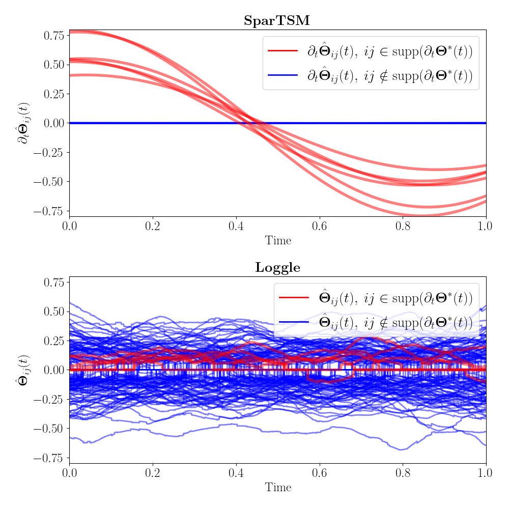
Figure 1: SparTSM compared with Loggle. Estimating the differential parameter vs. Estimating the time-varying parameter.

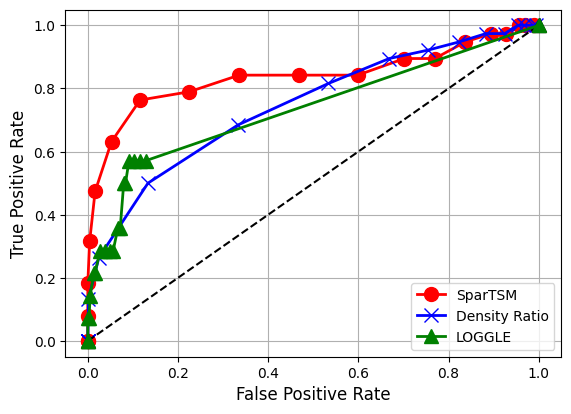
Figure 2: ROC of edge detection. The diagonal line has been added for reference.

We evaluate SparTSM and SparTSM+ estimator performance using datasets simulated with Gaussian Graphical Models (GGM). We sample $\boldsymbol{x}\sim\mathcal{N}(\boldsymbol{0},{\boldsymbol{\Theta}}^{-1})$ with ${\boldsymbol{\Theta}}(t)={\boldsymbol{\Theta}}_{0}+{\boldsymbol{\Theta}}^{\prime}(t)$, where ${\boldsymbol{\Theta}}_{0}$ is a constant symmetric positive definite dense matrix, and ${\boldsymbol{\Theta}}^{\prime}(t)$ is a sparse symmetric matrix that changes over time. Refer to Appendix G for settings of ${\boldsymbol{\Theta}}^{\prime}(t)$ in each experiment.

7.1 Differential Parameters Estimation using SparTSM

We generate 5000 synthetic samples from a 20-node Gaussian Graphical Model (GGM) and conduct a performance comparison between Loggle (Yang and Peng,, 2020), which is designed to capture smoothly varying $\boldsymbol{\Theta}(t)$, and SparTSM. In this study, the non-zero elements of ${\boldsymbol{\Theta}}^{\prime}(t)$ are formulated using a sine function (refer to Section G.1). In Figure 1, we illustrate the estimated $\partial_{t}\Theta_{i,j}(t)$ using SparTSM and the estimated $\Theta_{i,j}(t)$ with Loggle. The true time-variant parameters (where $\partial_{t}\Theta_{i,j}(t)\neq 0$) are marked in red. On one hand, SparTSM, utilizing an appropriate basis function (Fourier basis function), succeeds in accurately estimating differential parameters, thereby clearly identifying the transitions in the time-variant distribution. Conversely, Loggle struggles to discern any such parameters as its estimates are conflated. This aligns with expectations, since our constructed $\boldsymbol{\Theta}(t)$ is consistently non-sparse, requiring the estimation of a dense parameter vector, which does not adhere to Loggle’s sparsity assumptions. In experiments below, we set $\phi(t)=t$.

We quantitatively evaluate SparTSM’s effectiveness in detecting parameter changes by comparing it to Loggle and the density ratio-based method Liu et al., (2017); Kim et al., (2021), using ROC curves for assessment. We use a GGM that changes linearly with 40 nodes and 1000 samples (Details can be found in G.1). For the density ratio approach, ${\boldsymbol{\Theta}}(1)-{\boldsymbol{\Theta}}(0)$ is calculated by estimating the ratio $q_{1}/q_{0}$, where we draw 500 samples from $q_{0}$ and 500 samples from $q_{1}$. By adjusting the regularization parameter in both SparTSM and the density ratio approach, we can modify the number of changes detected, resulting in an ROC curve. In contrast, Loggle does not directly provide $\partial_{t}\Theta_{i,j}(t)$, but rather offers a timeline of $\Theta_{i,j}(t)$ values. Since $\Theta_{i,j}(t)$ follows a linear trend, we estimate the time derivative using the slope from least square regression (see Section G.5). Different detection thresholds then yield a series of sensitivity levels. The ROC curves are displayed in Figure 2, demonstrating that SparTSM’s ROC curve outperforms the others in this context, reflecting its superior efficacy.

7.2 Differential Parameter Inference using SparTSM+

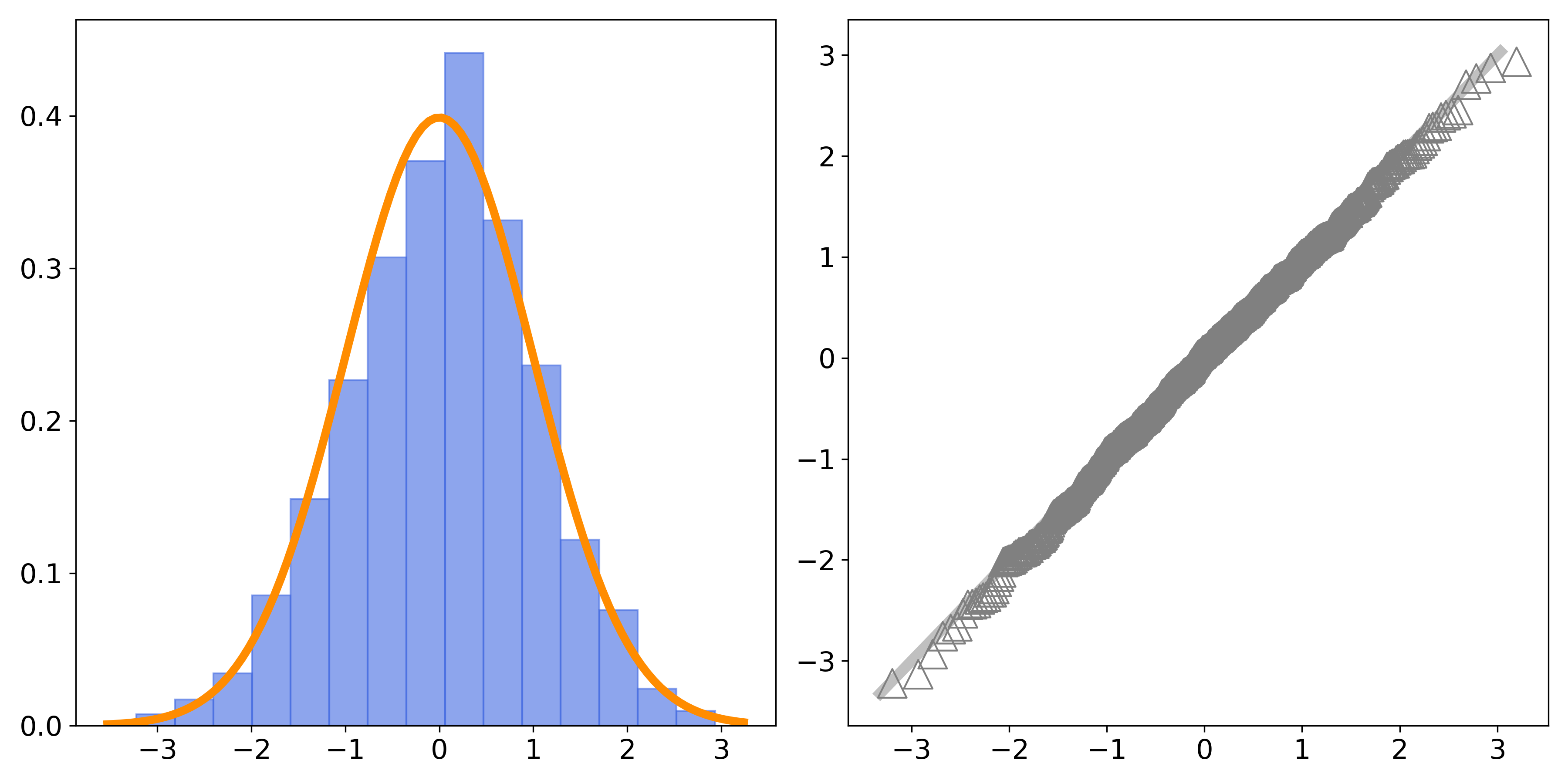
Figure 3: Gaussian approximation of SparTSM+

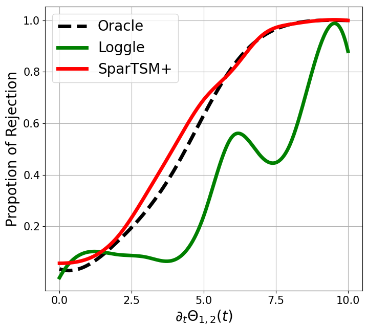
Figure 4: Power plot. $\mathcal{H}_{0}:\partial_{t}\Theta_{1,2}(t)=0$.

Variants	Deterministic	Random
Loggle (Yang and Peng,, 2020)	4.0%	6.0%
Oracle	3.4%	2.2%
SparTSM+	5.6%	5.3%

Table 1: The proportions of unsuccessful coverage at nominal confidence level of $95\%$. $\mathcal{H}_{0}:\partial_{t}\Theta_{1,2}(t)=0$.

In exploring SparTSM+, we assess it using two distinct linear GGM datasets, with details provided in Section G.2. We create 400 samples and 20 nodes from both fixed and random precision matrices, execute SparTSM+ 1000 times, and depict the distribution of $(\tilde{\alpha}_{1,2}-\alpha^{*}_{1,2})/{\hat{\sigma}_{1,2}}$ in Figure 3. This showcases the effectiveness of the Gaussian approximation for the standardized SparTSM+. The histogram closely aligns with the standard normal density function. In the Q-Q plot, data points align with or are near the reference line, underscoring the high precision of the Gaussian approximation and reinforcing Theorems 6.5 and 6.7 through our experimental results.

We further compare SparTSM+ against the Oracle method and Loggle regarding confidence interval coverage across 1000 iterations. The Oracle approach presupposes known sparsity of elements and constructs confidence intervals using the asymptotic variance of an M-estimator (van der Vaart,, 1998). Loggle’s confidence intervals are derived from the $2.5\%$ and $97.5\%$ quantiles of the test statistic (estimated slope) from 100 permutation tests.

Table 1 shows the proportions of failure in achieving the nominal confidence level of $95\%$. Even with limited sample sizes, SparTSM+ maintains coverage close to the intended level, whereas the oracle is more conservative. Notably, our heuristic method for determining the confidence interval for Loggle also achieves fairly reliable coverage. Nonetheless, the permutation test is computationally intensive in practice.

As illustrated in Figure 4, the power of tests is demonstrated for $\partial_{t}\Theta_{1,2}(t)$ values between 0 and 10. The power is calculated as the ratio of rejections across 1000 independent trials at a significance level of $0.05$ under the null hypothesis $\mathcal{H}_{0}:\partial_{t}\Theta_{1,2}(t)=0$. It is evident that as $\partial_{t}\Theta_{1,2}(t)$ varies from $\mathcal{H}_{0}$, the rejection rate of our proposed method escalates, showcasing the test’s efficacy. Notably, the proposed method usually provides greater power than the oracle, emphasizing its effectiveness in high-dimensional contexts.

8 Application: 109th US Senate

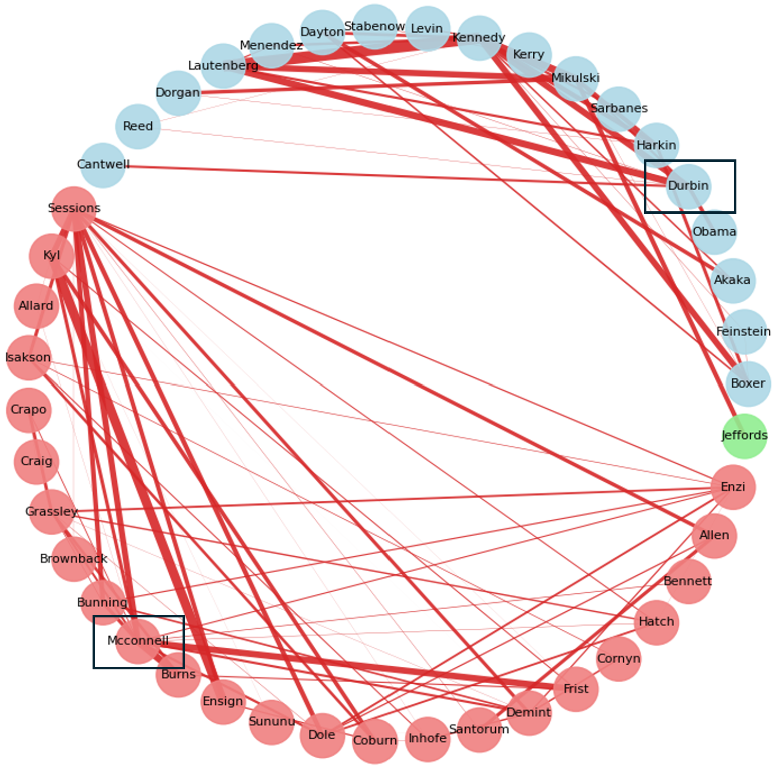
Figure 5: The differential graph estimated from 109th senate voting dataset. Red edge indicate a positive $\alpha_{i,j}\approx\partial_{t}\Theta_{i,j}(t)$. The widths of edges are proportional to $|\alpha_{i,j}|$. Democrats, republicans, independents are colored in blue, red and green respectively. Party whips are marked by a black rectangle.

We employ SparTSM on the voting data from the 109th US Senate (Roy et al.,, 2016), which encapsulates the choices made by 100 senators over around two years. The data is organized as $\mathcal{D}=\{(t_{i},\boldsymbol{x}_{i})\}_{i=1}^{427},\boldsymbol{x}_{i}\in\{0,1\}^{100},$ where ‘1’ signifies a yea vote and ‘0’ represents a nay vote. We consider these votes to adhere to a pairwise, time-dependent Ising model, described as $q_{t}\propto\exp\left(\sum_{i,j}\Theta_{i,j}(t)x_{i}x_{j}\right)$, and utilize SparTSM to compute $\partial_{t}\Theta_{i,j}(t)$ with a linear model $\phi(t)=t$. The parameter $\lambda_{\mathrm{lasso}}$ is adjusted to ensure fewer than 100 non-zero elements remain in ${\boldsymbol{\alpha}}$. In Figure 5, we illustrate the differential graph $G=(V,E)$, where $E:=\{(V_{i},V_{j})|\hat{\alpha}_{i,j}\neq 0\}$, meaning the edges denote variations in pairwise interactions within the Ising model. Nodes without connections are excluded.

Notably, all calculated $\hat{\alpha}_{i,j}$ values are positive and occur within the same party. This suggests that as the congressional term advances, senators increasingly align their votes with key party figures (like whips), creating “voting blocks” within the party. Furthermore, there is no apparent bipartisanship emerging between parties. In summary, these findings demonstrate a rise in partisanship throughout the congressional term.

Appendix A Notations

We denote $\|\cdot\|$ as a norm on $\mathbb{R}^{k}$ and use $\|\boldsymbol{v}\|_{l}=\left({\sum_{i=1}^{k}|v_{i}|^{l}}\right)^{1/l}$ as an usual $\ell_{l}$ norm for $l\in[1,\infty]$ and $\|\boldsymbol{v}\|_{0}=|\text{supp}(\boldsymbol{v})|=|\{i:v_{i}\neq 0\}|$; for a matrix $\boldsymbol{M}\in\mathbb{R}^{k\times k}$, $\|\boldsymbol{M}\|=\|\text{Vec}(\boldsymbol{M})\|$; $\text{For }l>0$, $|||\boldsymbol{M}|||_{l}=\sup_{\|v\|_{0}\leq l,\|v\|=1}|v^{\top}\boldsymbol{M}v|$ is the maximum $l$-sparse eigenvalue of $\boldsymbol{M}$; consequently, $|||\boldsymbol{M}|||_{\infty}=\sup_{\|\boldsymbol{v}\|\leq 1}\|\boldsymbol{Mv}\|_{\infty}$.

Appendix B Proof of Theorem 3.1

Recall that

$$q(\boldsymbol{x};\boldsymbol{\theta}^{*}(t))=\frac{\exp\left(\left\langle\boldsymbol{\theta}^{*}(t),\boldsymbol{f}(\boldsymbol{x})\right\rangle\right)}{Z(\boldsymbol{\theta}^{*}(t))}.$$

Thus,

$$\partial_{t}\log q(\boldsymbol{x};\boldsymbol{\theta}^{*}(t)) =\partial_{t}\left\langle\boldsymbol{\theta}^{*}(t),\boldsymbol{f}(\boldsymbol{x})\right\rangle-\partial_{t}\log Z(\boldsymbol{\theta}^{*}(t))$$

$$=\left\langle\partial_{t}\boldsymbol{\theta}^{*}(t),\boldsymbol{f}(\boldsymbol{x})\right\rangle-\frac{\partial_{t}Z(\boldsymbol{\theta}^{*}(t))}{Z(\boldsymbol{\theta}^{*}(t))}$$

$$=\left\langle\partial_{t}\boldsymbol{\theta}^{*}(t),\boldsymbol{f}(\boldsymbol{x})\right\rangle-\frac{\partial_{t}\int_{\mathcal{X}}\exp\left(\left\langle\boldsymbol{\theta}^{*}(t),\boldsymbol{f}(\boldsymbol{x})\right\rangle\right)d\boldsymbol{x}}{Z(\boldsymbol{\theta}^{*}(t))}$$

$$=\left\langle\partial_{t}\boldsymbol{\theta}^{*}(t),\boldsymbol{f}(\boldsymbol{x})\right\rangle-\frac{\int_{\mathcal{X}}\partial_{t}\left\langle\boldsymbol{\theta}^{*}(t),\boldsymbol{f}(\boldsymbol{x})\right\rangle\exp\left(\left\langle\boldsymbol{\theta}^{*}(t),\boldsymbol{f}(\boldsymbol{x})\right\rangle\right)d\boldsymbol{x}}{Z(\boldsymbol{\theta}^{*}(t))}$$

$$=\left\langle\partial_{t}\boldsymbol{\theta}^{*}(t),\boldsymbol{f}(\boldsymbol{x})\right\rangle-\frac{\int_{\mathcal{X}}\left\langle\partial_{t}\boldsymbol{\theta}^{*}(t),\boldsymbol{f}(\boldsymbol{x})\right\rangle\exp\left(\left\langle\boldsymbol{\theta}^{*}(t),\boldsymbol{f}(\boldsymbol{x})\right\rangle\right)d\boldsymbol{x}}{Z(\boldsymbol{\theta}^{*}(t))}$$

$$=\left\langle\partial_{t}\boldsymbol{\theta}^{*}(t),\boldsymbol{f}(\boldsymbol{x})\right\rangle-\int_{\mathcal{X}}\left\langle\partial_{t}\boldsymbol{\theta}^{*}(t),\boldsymbol{f}(\boldsymbol{x})\right\rangle\frac{\exp\left(\left\langle\boldsymbol{\theta}^{*}(t),\boldsymbol{f}(\boldsymbol{x})\right\rangle\right)}{Z(\boldsymbol{\theta}^{*}(t))}d\boldsymbol{x}$$

$$=\left\langle\partial_{t}\boldsymbol{\theta}^{*}(t),\boldsymbol{f}(\boldsymbol{x})\right\rangle-\int_{\mathcal{X}}\left\langle\partial_{t}\boldsymbol{\theta}^{*}(t),\boldsymbol{f}(\boldsymbol{x})\right\rangle q(\boldsymbol{x};\boldsymbol{\theta}^{*}(t))d\boldsymbol{x}$$

$$=\left\langle\partial_{t}\boldsymbol{\theta}^{*}(t),\boldsymbol{f}(\boldsymbol{x})\right\rangle-\mathbb{E}_{q_{t}}\left[\left\langle\partial_{t}\boldsymbol{\theta}^{*}(t),\boldsymbol{f}(\boldsymbol{x})\right\rangle\right],$$

as desired.

Appendix C Proof of Theorem 4.1

Let us begin from the initial formulation of our time based score matching objective with weight function $g(t)=g(t)$ for which $g(0)=g(1)=0$, i.e. $g(t)=0$ at the edges of our time domain $t\in[0,1]$. The initial objective is given by

$$\mathcal{L}(\partial_{t}{\boldsymbol{\theta}}(t)) =\int_{t=0}^{t=1}\mathbb{E}_{q_{t}}\left[g(t)\|\partial_{t}\log{q_{t}}({\boldsymbol{x}})-s_{t}\|^{2}\right]dt$$

$$=\int_{t=0}^{t=1}\mathbb{E}_{q_{t}}\left[g(t)s_{t}^{2}\right]dt-2\int_{t=0}^{t=1}\mathbb{E}_{q_{t}}\left[g(t)s_{t}\partial_{t}\log{q_{t}}({\boldsymbol{x}})\right]dt+\int_{t=0}^{t=1}\mathbb{E}_{q_{t}}\left[g(t)\partial_{t}\log{q_{t}}({\boldsymbol{x}})^{2}\right]dt$$

$$=\int_{t=0}^{t=1}\mathbb{E}_{q_{t}}\left[g(t)s_{t}^{2}\right]dt-2\int_{t=0}^{t=1}\int_{\mathcal{X}}\left[q_{t}\partial_{t}\log{q_{t}}({\boldsymbol{x}})\right]g(t)s_{t}d\boldsymbol{x}dt+\int_{t=0}^{t=1}\mathbb{E}_{q_{t}}\left[g(t)\partial_{t}\log{q_{t}}({\boldsymbol{x}})^{2}\right]dt$$

$$=\int_{t=0}^{t=1}\mathbb{E}_{q_{t}}\left[g(t)s_{t}^{2}\right]dt-2\int_{t=0}^{t=1}\int_{\mathcal{X}}\partial_{t}q_{t}g(t)s_{t}d\boldsymbol{x}dt+\int_{t=0}^{t=1}\mathbb{E}_{q_{t}}\left[g(t)\partial_{t}\log{q_{t}}({\boldsymbol{x}})^{2}\right]dt,$$

where in the final line we have used $q_{t}\partial_{t}\log{q_{t}}({\boldsymbol{x}})=q_{t}\partial_{t}\log q_{t}=\partial_{t}q_{t}$ to simplify. First note that the final term is a constant with respect to the model $s_{t}$, and so we can write $C=\int_{t=0}^{t=1}\mathbb{E}_{q_{t}}\left[g(t)\partial_{t}\log{q_{t}}({\boldsymbol{x}})^{2}\right]dt$. We continue by expanding the middle term via integration by parts

$$\mathcal{L}(\partial_{t}{\boldsymbol{\theta}}(t)) =\int_{t=0}^{t=1}\mathbb{E}_{q_{t}}\left[g(t)s_{t}^{2}\right]dt-2\left[\int_{\mathcal{X}}q_{t}g(t)s_{t}d\boldsymbol{x}\right]^{t=1}_{t=0}+2\int_{t=0}^{t=1}\int_{\mathcal{X}}q_{t}\partial_{t}(g(t)s_{t})d\boldsymbol{x}dt+C$$

$$=\int_{t=0}^{t=1}\mathbb{E}_{q_{t}}\left[g(t)s_{t}^{2}\right]dt+2\int_{t=0}^{t=1}\int_{\mathcal{X}}q_{t}\partial_{t}(g(t)s_{t})d\boldsymbol{x}dt+C$$

$$=\int_{t=0}^{t=1}g(t)\mathbb{E}_{q_{t}}\left[s_{t}^{2}\right]dt+2\int_{t=0}^{t=1}\partial_{t}g(t)\mathbb{E}_{q_{t}}\left[s_{t}\right]dt+2\int_{t=0}^{t=1}g(t)\mathbb{E}_{q_{t}}\left[\partial_{t}s_{t}\right]dt+C,$$ (20)

where the second equality is due to $\left[\int_{\mathcal{X}}q_{t}g(t)s_{t}d\boldsymbol{x}\right]^{t=1}_{t=0}=0$ as $g(0)=g(1)=0$.

Let us now substitute the model given in Equation 3, stated again here for completeness, given by

$$s_{t}=s(\boldsymbol{x};t)=\left\langle\partial_{t}\boldsymbol{\theta}(t),\boldsymbol{f}(\boldsymbol{x})\right\rangle-\mathbb{E}_{q_{t}}\left[\left\langle\partial_{t}\boldsymbol{\theta}(t),\boldsymbol{f}(\boldsymbol{x})\right\rangle\right].$$

We calculate $\mathbb{E}_{q_{t}}\left[s_{t}\right]$ and $\mathbb{E}_{q_{t}}\left[\partial_{t}s_{t}\right]$ to substitute into the equation above. These are given by

$$\mathbb{E}_{q_{t}}\left[s_{t}\right] =\mathbb{E}_{q_{t}}\left[\left\langle\partial_{t}\boldsymbol{\theta}(t),\boldsymbol{f}(\boldsymbol{x})\right\rangle-\mathbb{E}_{q_{t}}\left[\left\langle\partial_{t}\boldsymbol{\theta}(t),\boldsymbol{f}(\boldsymbol{x})\right\rangle\right]\right]$$

$$=\mathbb{E}_{q_{t}}\left[\left\langle\partial_{t}\boldsymbol{\theta}(t),\boldsymbol{f}(\boldsymbol{x})\right\rangle\right]-\mathbb{E}_{q_{t}}\left[\left\langle\partial_{t}\boldsymbol{\theta}(t),\boldsymbol{f}(\boldsymbol{x})\right\rangle\right]$$

$$=0$$

$$\mathbb{E}_{q_{t}}\left[\partial_{t}s_{t}\right] =\mathbb{E}_{q_{t}}\left[\partial_{t}\left(\left\langle\partial_{t}\boldsymbol{\theta}(t),\boldsymbol{f}(\boldsymbol{x})\right\rangle-\mathbb{E}_{q_{t}}\left[\left\langle\partial_{t}\boldsymbol{\theta}(t),\boldsymbol{f}(\boldsymbol{x})\right\rangle\right]\right)\right]$$

$$=\mathbb{E}_{q_{t}}\left[\left\langle\partial_{t}^{2}\boldsymbol{\theta}_{t},\boldsymbol{f}(\boldsymbol{x})\right\rangle-\partial_{t}\left(\mathbb{E}_{q_{t}}\left[\left\langle\partial_{t}\boldsymbol{\theta}(t),\boldsymbol{f}(\boldsymbol{x})\right\rangle\right]\right)\right]$$

$$=\mathbb{E}_{q_{t}}\left[\left\langle\partial_{t}^{2}\boldsymbol{\theta}_{t},\boldsymbol{f}(\boldsymbol{x})\right\rangle-\partial_{t}\left(\int_{\mathcal{X}^{\prime}}q_{t}\left\langle\partial_{t}\boldsymbol{\theta}(t),\boldsymbol{f}(\boldsymbol{x})\right\rangle d\boldsymbol{x}^{\prime}\right)\right]$$

$$=\mathbb{E}_{q_{t}}\left[\left\langle\partial_{t}^{2}\boldsymbol{\theta}_{t},\boldsymbol{f}(\boldsymbol{x})\right\rangle-\int_{\mathcal{X}^{\prime}}\partial_{t}q_{t}\left\langle\partial_{t}\boldsymbol{\theta}(t),\boldsymbol{f}(\boldsymbol{x})\right\rangle d\boldsymbol{x}^{\prime}-\int_{\mathcal{X}^{\prime}}q_{t}\left\langle\partial_{t}^{2}\boldsymbol{\theta}_{t},\boldsymbol{f}(\boldsymbol{x})\right\rangle d\boldsymbol{x}^{\prime}\right]$$

$$=\mathbb{E}_{q_{t}}\left[\left\langle\partial_{t}^{2}\boldsymbol{\theta}_{t},\boldsymbol{f}(\boldsymbol{x})\right\rangle-\int_{\mathcal{X}^{\prime}}\partial_{t}q_{t}\left\langle\partial_{t}\boldsymbol{\theta}(t),\boldsymbol{f}(\boldsymbol{x})\right\rangle d\boldsymbol{x}^{\prime}-\mathbb{E}_{q_{t}}{\left\langle\partial_{t}^{2}\boldsymbol{\theta}_{t},\boldsymbol{f}(\boldsymbol{x})\right\rangle d\boldsymbol{x}^{\prime}}\right]$$

$$=\mathbb{E}_{q_{t}}\left[\left\langle\partial_{t}^{2}\boldsymbol{\theta}_{t},\boldsymbol{f}(\boldsymbol{x})\right\rangle-\int_{\mathcal{X}^{\prime}}\partial_{t}q_{t}\left\langle\partial_{t}\boldsymbol{\theta}(t),\boldsymbol{f}(\boldsymbol{x})\right\rangle d\boldsymbol{x}^{\prime}\right]-\mathbb{E}_{q_{t}}\left[\left\langle\partial_{t}^{2}\boldsymbol{\theta}_{t},\boldsymbol{f}(\boldsymbol{x})\right\rangle d\boldsymbol{x}^{\prime}\right]$$

$$=\mathbb{E}_{q_{t}}\left[-\int_{\mathcal{X}^{\prime}}\partial_{t}q_{t}\left\langle\partial_{t}\boldsymbol{\theta}(t),\boldsymbol{f}(\boldsymbol{x})\right\rangle d\boldsymbol{x}^{\prime}\right],$$

where the integral $\int_{\mathcal{X}^{\prime}}(\dots)d\boldsymbol{x}^{\prime}$ is the same integral as $\int_{\mathcal{X}}(\dots)d\boldsymbol{x}$ but written as such to make them distinct from one another. Substituting these into Equation 20 gives

$$\mathcal{L}(\partial_{t}{\boldsymbol{\theta}}(t)) =\int_{t=0}^{t=1}g(t)\mathbb{E}_{q_{t}}\left[s_{t}^{2}\right]dt-2\int_{t=0}^{t=1}g(t)\mathbb{E}_{q_{t}}\left[\int_{\mathcal{X}^{\prime}}\partial_{t}q_{t}\left\langle\partial_{t}\boldsymbol{\theta}(t),\boldsymbol{f}(\boldsymbol{x})\right\rangle d\boldsymbol{x}^{\prime}\right]dt+C$$

$$=\int_{t=0}^{t=1}g(t)\mathbb{E}_{q_{t}}\left[s_{t}^{2}\right]dt-2\int_{t=0}^{t=1}g(t)\int_{\mathcal{X}}q_{t}\left(\int_{\mathcal{X}^{\prime}}\partial_{t}q_{t}\left\langle\partial_{t}\boldsymbol{\theta}(t),\boldsymbol{f}(\boldsymbol{x})\right\rangle d\boldsymbol{x}^{\prime}\right)d\boldsymbol{x}dt+C$$

$$\stackrel{{\scriptstyle\mathclap{\tiny\mbox{(a)}}}}{{=}}\int_{t=0}^{t=1}g(t)\mathbb{E}_{q_{t}}\left[s_{t}^{2}\right]dt-2\int_{t=0}^{t=1}g(t)\left(\int_{\mathcal{X}}q_{t}d\boldsymbol{x}\right)\int_{\mathcal{X}^{\prime}}\partial_{t}q_{t}\left\langle\partial_{t}\boldsymbol{\theta}(t),\boldsymbol{f}(\boldsymbol{x})\right\rangle d\boldsymbol{x}^{\prime}dt+C$$

$$\stackrel{{\scriptstyle\mathclap{\tiny\mbox{(b)}}}}{{=}}\int_{t=0}^{t=1}g(t)\mathbb{E}_{q_{t}}\left[s_{t}^{2}\right]dt-2\int_{t=0}^{t=1}g(t)\int_{\mathcal{X}}\partial_{t}q_{t}\left\langle\partial_{t}\boldsymbol{\theta}(t),\boldsymbol{f}(\boldsymbol{x})\right\rangle d\boldsymbol{x}dt+C.$$

In the equality denoted by (a), we have used the fact that inside the integral $\int_{\mathcal{X}}q_{t}(\dots)d\boldsymbol{x}$ the only variable dependent on $\boldsymbol{x}$ was $q_{t}$, as $\boldsymbol{x}$ and $\boldsymbol{x}^{\prime}$ are independent. We also have that $\int_{\mathcal{X}}q_{t}d\boldsymbol{x}=1$ by $q_{t}$ being a probability density function. The equality denoted by (b) contains a re-labelling of $\mathcal{X}=\mathcal{X}^{\prime}$ and $\boldsymbol{x}=\boldsymbol{x}^{\prime}$, as they are the same variable, only labelled differently originally to make them distinct. We use integration by parts one final time to obtain

$$\mathcal{L}(\partial_{t}{\boldsymbol{\theta}}(t)) =\int_{t=0}^{t=1}g(t)\mathbb{E}_{q_{t}}\left[s_{t}^{2}\right]dt-2\left[\int_{\mathcal{X}}q_{t}g(t)\left\langle\partial_{t}\boldsymbol{\theta}(t),\boldsymbol{f}(\boldsymbol{x})\right\rangle d\boldsymbol{x}\right]^{t=1}_{t=0}+2\int_{t=0}^{t=1}\int_{\mathcal{X}}q_{t}\partial_{t}\left(g(t)\left\langle\partial_{t}\boldsymbol{\theta}(t),\boldsymbol{f}(\boldsymbol{x})\right\rangle\right)d\boldsymbol{x}dt+C$$

$$=\int_{t=0}^{t=1}g(t)\mathbb{E}_{q_{t}}\left[s_{t}^{2}\right]dt+2\int_{t=0}^{t=1}\int_{\mathcal{X}}q_{t}\partial_{t}\left(g(t)\left\langle\partial_{t}\boldsymbol{\theta}(t),\boldsymbol{f}(\boldsymbol{x})\right\rangle\right)d\boldsymbol{x}dt+C,$$

using again that $g(0)=g(1)=0$, and finally

$$\mathcal{L}(\partial_{t}{\boldsymbol{\theta}}(t)) =\int_{t=0}^{t=1}g(t)\mathbb{E}_{q_{t}}\left[s_{t}^{2}\right]dt+2\int_{t=0}^{t=1}\int_{\mathcal{X}}q_{t}\partial_{t}g(t)\left\langle\partial_{t}\boldsymbol{\theta}(t),\boldsymbol{f}(\boldsymbol{x})\right\rangle d\boldsymbol{x}dt+2\int_{t=0}^{t=1}\int_{\mathcal{X}}q_{t}g(t)\left\langle\partial_{t}^{2}\boldsymbol{\theta}_{t},\boldsymbol{f}(\boldsymbol{x})\right\rangle d\boldsymbol{x}dt+C$$

$$=\int_{t=0}^{t=1}\mathbb{E}_{q_{t}}\left[g(t)s_{t}^{2}+2\partial_{t}g(t)\left\langle\partial_{t}\boldsymbol{\theta}(t),\boldsymbol{f}(\boldsymbol{x})\right\rangle+2g(t)\left\langle\partial_{t}^{2}\boldsymbol{\theta}_{t},\boldsymbol{f}(\boldsymbol{x})\right\rangle\right]dt$$

which is the same as Equation 5 in the main text.

Appendix D Finite-sample Estimation Error of Lasso Estimator

An equivalent sample objective function is as the following:

$$\hat{\mathcal{L}}(\boldsymbol{\alpha})=\frac{1}{2n}\left[\boldsymbol{\alpha}\tilde{\boldsymbol{F}}^{\top}\boldsymbol{G}\tilde{\boldsymbol{F}}\boldsymbol{\alpha}^{\top}+2\boldsymbol{1}_{n}^{\top}\partial_{t}\boldsymbol{G}{\boldsymbol{F}}\boldsymbol{\alpha}^{\top}\right]$$ (21)

where diagonal matrix $\boldsymbol{G},\partial_{t}\boldsymbol{G}\in\mathbb{R}^{n\times n}$ with $i$-th diagonal entry to be $g(t_{i})$ and $\partial_{t}g(t_{i})$ respectively.

Theorem D.1.

Suppose Assumption 6.1 and 6.3 hold. Any minimizer of the objective function Equation 11 with regularization parameter lower bounded as $\lambda_{\mathrm{lasso}}\geq 2\left\|\nabla_{\boldsymbol{\alpha}}\hat{\mathcal{L}}(\boldsymbol{\alpha}^{*})\right\|_{\infty}$ satisfies

$$||\hat{\boldsymbol{\alpha}}-\boldsymbol{\alpha}^{*}||_{2}\leq\frac{3}{\kappa}{\|{\boldsymbol{\alpha}}^{*}\|_{0}^{1/2}}\lambda_{\mathrm{lasso}},~{}~{}~{}||\hat{\boldsymbol{\alpha}}-\boldsymbol{\alpha}^{*}||_{1}\leq\frac{6}{\kappa}\|{\boldsymbol{\alpha}}^{*}\|_{0}\lambda_{\mathrm{lasso}}.$$ (22)

D.1 Proof of Theorem D.1

Following equation 21 and Assumption 6.1, we can express the second order Taylor polynomial around $\boldsymbol{\alpha}^{*}$ as follows:

$$\hat{\mathcal{L}}(\hat{\boldsymbol{\alpha}})=\hat{\mathcal{L}}(\boldsymbol{\alpha}^{*})+\frac{1}{n}\left[\boldsymbol{\alpha}^{*}{\tilde{\boldsymbol{F}}}^{\top}\boldsymbol{G}{\tilde{\boldsymbol{F}}}\boldsymbol{+}\boldsymbol{1}_{n}^{\top}\partial_{t}\boldsymbol{G}{\boldsymbol{F}}\right](\boldsymbol{\hat{\alpha}}-\boldsymbol{\alpha}^{*})^{\top}+\frac{1}{2n}(\boldsymbol{\hat{\alpha}}-\boldsymbol{\alpha}^{*})\left[{\tilde{\boldsymbol{F}}}^{\top}\boldsymbol{G}{\tilde{\boldsymbol{F}}}\right](\hat{\boldsymbol{\alpha}}-\boldsymbol{\alpha}^{*})^{\top}$$ (23)

where the residual $R_{2}(\hat{\boldsymbol{\alpha}},\boldsymbol{\alpha}^{*})=0$ since $\hat{\mathcal{L}}$ quadratic.

Lemma D.2.

Under condition $\lambda_{\mathrm{lasso}}\geq 2\left\|\nabla_{\boldsymbol{\alpha}}\hat{\mathcal{L}}(\boldsymbol{\alpha}^{*})\right\|_{\infty}$, the error vector $\widehat{\Delta}=\hat{\boldsymbol{\alpha}}-\boldsymbol{\alpha}^{*}\in\mathbb{C}_{3}(S)$

Proof.

Since $\hat{\boldsymbol{\alpha}}$ is optimal, we have

$$\hat{\mathcal{L}}(\hat{\boldsymbol{\alpha}})+\lambda_{\mathrm{lasso}}||\hat{\boldsymbol{\alpha}}||_{1}\leq\hat{\mathcal{L}}(\boldsymbol{\alpha}^{*})+\lambda_{\mathrm{lasso}}||{\boldsymbol{\alpha}}^{*}||_{1}$$ (24)

Rearranging we have from second order Taylor approximation:

$$0\leq\frac{1}{2n}||G^{\frac{1}{2}}{\tilde{\boldsymbol{F}}}\hat{\Delta}^{\top}||_{2}^{2}\leq\frac{1}{n}|\nabla_{\boldsymbol{\alpha}}\hat{\mathcal{L}}(\boldsymbol{\alpha}^{*})\hat{\Delta}^{\top}|+\lambda_{\mathrm{lasso}}\{||\boldsymbol{\alpha}^{*}||_{1}-||\hat{\boldsymbol{\alpha}}||_{1}\}$$ (25)

where $|\cdot|$ denote the absolute value. Now since $\boldsymbol{\alpha}^{*}$ is $S$-sparse, we can write

$$\|\boldsymbol{\alpha}^{*}\|_{1}-\|\hat{\boldsymbol{\alpha}}\|_{1}=\|\boldsymbol{\alpha}_{S}^{*}\|_{1}-\|\boldsymbol{\alpha}_{S}^{*}+\widehat{\Delta}_{S}\|_{1}-\|\widehat{\Delta}_{S^{c}}\|_{1}.$$ (26)

Using Holder’s inequality and the triangle inequality, we have

$$0 \leq\frac{1}{n}||G^{\frac{1}{2}}{\tilde{\boldsymbol{F}}}\hat{\Delta}^{\top}||_{2}^{2}\leq 2|\nabla_{\boldsymbol{\alpha}}\hat{\mathcal{L}}(\boldsymbol{\alpha}^{*})\hat{\Delta}^{\top}|+2\lambda_{\mathrm{lasso}}\{\|\boldsymbol{\alpha}_{S}^{*}\|_{1}-\|\boldsymbol{\alpha}^{*}_{S}+\widehat{\Delta}_{S}\|_{1}-\|\widehat{\Delta}_{S^{c}}\|_{1}\}$$ (27)

$$\leq 2\|\nabla_{\boldsymbol{\alpha}}\hat{\mathcal{L}}(\boldsymbol{\alpha}^{*})\|_{\infty}\|\widehat{\Delta}\|_{1}+2\lambda_{\mathrm{lasso}}\{\|\widehat{\Delta}_{S}\|_{1}-\|\widehat{\Delta}_{S^{c}}\|_{1}\}$$ (28)

$$\leq\lambda_{\mathrm{lasso}}\{3\|\widehat{\Delta}_{S}\|_{1}-\|\widehat{\Delta}_{S^{c}}\|_{1}\},$$ (29)

where last inequality shows that $\widehat{\Delta}\in\mathbb{C}_{3}(S)$. ∎

Lemma D.3.

$||\widehat{\Delta}||_{1}\leq 2\sqrt{s}||\widehat{\Delta}||_{2}$ where $s=|S|$.

Proof.

Since $S$ is the support of $\boldsymbol{\alpha}^{*}$

$$||\boldsymbol{\alpha}_{S}^{*}||_{1}=||\boldsymbol{\alpha}^{*}||_{1}\geq||\boldsymbol{\alpha}^{*}+\widehat{\Delta}||_{1}=||\boldsymbol{\alpha}_{S}^{*}+\widehat{\Delta}_{S}||_{1}+||\widehat{\Delta}_{S^{c}}||_{1}\geq||\boldsymbol{\alpha}^{*}_{S}||_{1}-||\widehat{\Delta}_{S}||_{1}+||\widehat{\Delta}_{S^{c}}||_{1}.$$ (30)

where we used the fact that $\boldsymbol{\alpha}_{S^{c}}^{*}=0$ and triangle inequality. This implies that $\widehat{\Delta}\in\mathbb{C}_{1}(S)$. Therefore

$$||\widehat{\Delta}||_{1}=||\widehat{\Delta}_{S}||_{1}+||\widehat{\Delta}_{S^{c}}||_{1}\leq 2||\widehat{\Delta}_{S}||_{1}\leq 2\sqrt{s}||\widehat{\Delta}||_{2}$$ (31)

∎

With all above, we can then apply the RE condition. Finally we have $||\widehat{\Delta}||_{2}^{2}\leq\frac{3}{\kappa}\lambda_{\mathrm{lasso}}\sqrt{s}||\widehat{\Delta}||_{2}$, which implies that

$$||\hat{\boldsymbol{\alpha}}-\boldsymbol{\alpha}^{*}||_{2}\leq\frac{3}{\kappa}\lambda_{\mathrm{lasso}}\sqrt{s}$$ (32)

D.2 Proof of Theorem 6.4

We have from definition that $\nabla_{\boldsymbol{\alpha}}\hat{\mathcal{L}}(\boldsymbol{\alpha})=\frac{1}{n}\sum_{j=1}^{n}\nabla_{\boldsymbol{\alpha}}\boldsymbol{m_{\alpha}}(t_{j},\boldsymbol{x}_{j})$.

Lemma D.4.

Under the condition that the r.v. $\boldsymbol{f}(x)$ is bounded in $\ell_{\infty}$ norm, let $\sigma^{2}=\max_{1\leq i\leq k}\boldsymbol{\Sigma}_{ii}$, where $\boldsymbol{\Sigma}$ is the covariance matrix of the random variable $\nabla_{\boldsymbol{\alpha}}\boldsymbol{m_{{\alpha}^{*}}}(t,\boldsymbol{x})$, the elements of $\nabla_{\boldsymbol{\alpha}}\hat{\mathcal{L}}(\boldsymbol{\alpha}^{*})$ follow a zero-mean sub-Gaussian distribution with parameter $\sigma^{2}/n$.

Proof.

(1) Proof the sub-Gaussian: let $|g(t)|\leq C_{g}\in\mathbb{R}_{+},|\partial_{t}g(t)|\leq C_{\partial_{t}g(t)}\in\mathbb{R}_{+},||\mathbb{E}_{q_{t}}[\boldsymbol{f}(x)]||_{\infty}\leq C_{E}\in\mathbb{R}_{+}$ and $||\boldsymbol{f}(x)||_{\infty}\leq C_{f}\in\mathbb{R}_{+}$ for $t\in[0,1]$. By using triangle inequality in $(i),(iii)$ and Cauchy-Schwarz inequality in $(ii)$ , we have by definition of $\nabla_{\boldsymbol{\alpha}}\boldsymbol{m_{\alpha}}(t,\boldsymbol{x})$

$$\left\|\nabla_{\boldsymbol{\alpha}}\boldsymbol{m_{\alpha}}(t,\boldsymbol{x})\right\|_{\infty}\leq\left\|\boldsymbol{\alpha}^{*}\right\|_{\infty}\left(C_{g}(C_{f}+C_{E})^{2}+C_{f}C_{\partial_{t}g(t)}\right)$$ (33)

therefore by $M=||\boldsymbol{\alpha}^{*}||(C_{g}(C_{f}+C_{E})^{2}+C_{f}C_{\partial_{t}g(t)})$ for simplicity

$$\left\|\nabla_{\boldsymbol{\alpha}}\hat{\mathcal{L}}\left(\boldsymbol{\alpha}^{*}\right)\right\|_{\infty}=\left\|\frac{1}{n}\sum_{j=1}^{n}\nabla_{\boldsymbol{\alpha}}\boldsymbol{m_{\alpha}}(t_{j},\boldsymbol{x}_{j})\right\|_{\infty}\leq M$$ (34)

which implies that $\nabla_{\boldsymbol{\alpha}}\hat{\mathcal{L}}(\boldsymbol{\alpha}^{*})$ is element-wise bounded hence all elements are sub-Gaussian by Hoeffding, (1994). Therefore, fixed number of data points $n$, then each element of $\nabla_{\boldsymbol{\alpha}}\hat{\mathcal{L}}(\boldsymbol{\alpha}^{*})$ follows a sub-Gaussian distribution with parameter $\sigma^{2}/n$ by addition rule of variance.
(2) Proof of zero-mean: We also assert that $\nabla_{\boldsymbol{\alpha}}\hat{\mathcal{L}}(\boldsymbol{\alpha}^{*})\in\mathbb{R}^{k}$ is a zero-mean random variable. Recall that the conditional density function $q(x|t)$ as $q_{t}(x)$ where $q_{t}:\mathbb{R}^{k}\rightarrow\mathbb{R}$ and $q:\mathbb{R}\rightarrow\mathbb{R}$ represent the density of $t$, where $t$ is uniformly distributed in the domain $[0,1]$, we then have the following:

$$\mathbb{E}_{x\sim q_{t}(x),\,t\sim q(t)}\left[\nabla_{\boldsymbol{\alpha}}\hat{\mathcal{L}}(\boldsymbol{\alpha}^{*})\right]$$

$$=\frac{1}{n}\mathbb{E}_{x\sim q_{t}(x),\,t\sim q(t)}\left[\boldsymbol{\alpha}^{*}{\tilde{\boldsymbol{F}}}^{\top}\boldsymbol{G}{\tilde{\boldsymbol{F}}}+\boldsymbol{1}_{n}^{\top}\partial_{t}\boldsymbol{G}\boldsymbol{F}\right]$$ (35)

$$\stackrel{{\scriptstyle(i)}}{{=}}\mathbb{E}_{x\sim q_{t}(x),\,t\sim q(t)}\left[\boldsymbol{{\alpha}^{*}}{\left(\boldsymbol{f}(x)-\mathbb{E}_{q_{t}}[\boldsymbol{f}(x)]\right)}g(t){\left(\boldsymbol{f}(x)-\mathbb{E}_{q_{t}}[\boldsymbol{f}(x)]\right)}+(\partial_{t}g(t))\boldsymbol{f}(x)\right]$$ (36)

$$=\int_{t}\int_{x}q(t)q_{t}(x)\{\boldsymbol{{\alpha}^{*}}{(\boldsymbol{f}(x)-\mathbb{E}_{q_{t}}[\boldsymbol{f}(x)])}g(t)\left(\boldsymbol{f}(x)-\mathbb{E}_{q_{t}}[\boldsymbol{f}(x)]\right)+(\partial_{t}g(t))\boldsymbol{f}(x)\}\mathrm{d}x\,\mathrm{d}t$$ (37)

$$\stackrel{{\scriptstyle(ii)}}{{=}}\int_{t}\int_{x}q_{t}(x)\{(\partial_{t}\log q_{t}(x))g(t)\left(\boldsymbol{f}(x)-\mathbb{E}_{q_{t}}[\boldsymbol{f}(x)]\right)+(\partial_{t}g(t))\boldsymbol{f}(x)\}\mathrm{d}x\,\mathrm{d}t$$ (38)

$$=\int_{t}\int_{x}(\partial_{t}q_{t}(x))g(t)\left(\boldsymbol{f}(x)-\mathbb{E}_{q_{t}}[\boldsymbol{f}(x)]\right)+q_{t}(x)(\partial_{t}g(t))\boldsymbol{f}(x)\}\mathrm{d}x\,\mathrm{d}t$$ (39)

$$=[q_{t}(x)g(t)\left(\boldsymbol{f}(x)-\mathbb{E}_{q_{t}}[\boldsymbol{f}(x)]\right)]^{t=1}_{t=0}-\int_{t}\int_{x}q_{t}(x)\partial_{t}\left[g(t)\left(\boldsymbol{f}(x)-\mathbb{E}_{q_{t}}[\boldsymbol{f}(x)]\right)\right]-q_{t}(x)(\partial_{t}g(t))\boldsymbol{f}(x)\mathrm{d}x\,\mathrm{d}t$$ (40)

$$\stackrel{{\scriptstyle(iii)}}{{=}}\int_{t}\int_{x}-q_{t}(x)\left[(\partial_{t}g(t))\left(\boldsymbol{f}(x)-\mathbb{E}_{q_{t}}[\boldsymbol{f}(x)]\right)-g(t)\partial_{t}\mathbb{E}_{q_{t}}\left[\boldsymbol{f}(x)\right]\right]+q_{t}(x)(\partial_{t}g(t))\boldsymbol{f}(x)\mathrm{d}x\,\mathrm{d}t$$ (41)

$$=\int_{t}\int_{x}q_{t}(x)\left([\partial_{t}g(t)]\mathbb{E}_{q_{t}}[\boldsymbol{f}(x)]+g(t)\partial_{t}\mathbb{E}_{q_{t}}[\boldsymbol{f}(x)]\right)\mathrm{d}x\,\mathrm{d}t=\int_{t}\int_{x}q_{t}(x)\partial_{t}[g(t)\mathbb{E}_{q_{t}}[\boldsymbol{f}(x)]]\mathrm{d}x\,\mathrm{d}t$$ (42)

$$=[q_{t}(x)g(t)\mathbb{E}_{q_{t}}[\boldsymbol{f}(x)]]^{t=1}_{t=0}-\int_{t}\int_{x}(\partial_{t}q_{t}(x))g(t)\mathbb{E}_{q_{t}}[\boldsymbol{f}(x)]\mathrm{d}x\,\mathrm{d}t$$ (43)

$$\stackrel{{\scriptstyle(iv)}}{{=}}-\int_{t}\partial_{t}\left(\int_{x}q_{t}(x)\mathrm{d}x\,\right)g(t)\mathbb{E}_{q_{t}}[\boldsymbol{f}(x)]\mathrm{d}t=\boldsymbol{0}$$ (44)

where $(i)$ follows that $\{f(x_{1}),..,f(x_{n})\}$ are i.i.d; $(ii)$ follows from the definition of $\partial_{t}\log q_{t}(x)$ and $q(t)=1$; $(iii),(iv)$ uses the boundary condition of $g(t)$. Therefore, each element of $\nabla_{\boldsymbol{\alpha}}\hat{\mathcal{L}}(\boldsymbol{\alpha}^{*})$ is a zero-mean sub-Gaussian r.v.

∎

Lemma D.5.

Let $J_{i}$ denotes i-th element of $\nabla_{\boldsymbol{\alpha}}\hat{\mathcal{L}}(\boldsymbol{\alpha}^{*})$, we have

$$\mathbb{E}[\max_{i\in[k]}|J_{i}|]\leq 2\sqrt{\frac{\sigma^{2}\log k}{n}}$$ (45)

Proof.

We have $\{J_{i}\}_{i=1}^{k}$ is a sequence of zero-mean random variables, each follows sub-Gaussian with parameter $\sigma^{2}/n$. For any $\lambda>0$, we can use the convexity of the exponential function to obtain

$$\exp\{\lambda\mathbb{E}[\max_{i\in[k]}J_{i}]\}\leq\mathbb{E}[\exp\{\lambda\max_{i\in[k]}J_{i}\}]$$

by Jensen’s inequality. And by the monotonicity of the exponential

$$\mathbb{E}[\exp\{\lambda\max_{i\in[k]}J_{i}\}]=\mathbb{E}[\max_{i\in[k]}e^{\lambda J_{i}}]\leq\sum_{i=1}^{k}\mathbb{E}[e^{\lambda J_{i}}]\leq ke^{\frac{\lambda^{2}\sigma^{2}}{2n}}.$$

where last inequality follows the definition of sub-Gaussian r.v. Therefore,

$$\mathbb{E}[\max_{i\in[k]}J_{i}]\leq\frac{\log k}{\lambda}+\lambda\frac{\sigma^{2}}{2n}$$

and $\lambda=\sqrt{\frac{2n\log k}{\sigma^{2}}}$ is optimal in $\lambda>0$; substituting we have

$$\mathbb{E}\left[\max_{i\in[k]}J_{i}\right]\leq\frac{\sigma}{\sqrt{2n}}\sqrt{\log k}+\frac{\sigma}{\sqrt{2n}}\sqrt{\log k}=\sqrt{2\sigma^{2}\log k/n}$$ (46)

Since 46 does not assume independence between individual $J_{i}$. The result follows by

$$\max_{i\in[k]}|J_{i}|=\max\{|J_{1}|,\ldots,|J_{k}|\}=\max\{J_{1},\ldots,J_{k},-J_{1},\ldots,-J_{k}\}$$

∎

Consequently, from standard sub-Gaussian tail bound and definition of $\ell_{\infty}$ norm, we have

$$\mathbb{P}\left[\left\|\nabla_{\boldsymbol{\alpha}}\hat{\mathcal{L}}(\boldsymbol{\alpha}^{*})\right\|_{\infty}\geq\sigma\left(\sqrt{\frac{2\log k}{n}}+\delta\right)\right]\leq 2e^{-\frac{n\delta^{2}}{2}}\;\;\text{for all }\delta>0$$ (47)

Hence if we set $\lambda_{\mathrm{lasso}}=2\sigma\left(\sqrt{\frac{2\log k}{n}}+\delta\right)$, then we have the probability that $\lambda_{\mathrm{lasso}}\geq 2||\nabla_{\boldsymbol{\alpha}}\hat{\mathcal{L}}(\boldsymbol{\alpha}^{*})||_{\infty}$ is in rate $1-2\exp\{-\Theta(n\delta^{2})\}$, which implies

$$||\hat{\boldsymbol{\alpha}}-\boldsymbol{\alpha}^{*}||_{2}\leq\frac{6}{\kappa}\sqrt{s}\sigma\left(\sqrt{\frac{2\log k}{n}}+\delta\right)$$ (48)

with probability greater than $1-2\exp\{-\frac{n\delta^{2}}{2}\}$ for all $\delta>0$.

Appendix E Theoretical Results of Debiased lasso

E.1 Variance Estimator

Lemma E.1.

$|||\hat{\boldsymbol{\Sigma}}(\hat{\boldsymbol{\alpha}})-\hat{\boldsymbol{\Sigma}}({\boldsymbol{\alpha}}^{*})|||_{\infty}\leq L||\hat{\boldsymbol{\alpha}}-\boldsymbol{\alpha}^{*}||_{1}$ where $L$ is a constant.

Proof.

Apply the fact that there exists $L_{0}$ such that $\|\nabla_{\boldsymbol{\alpha}}m(\hat{\boldsymbol{\alpha}})-\nabla_{\boldsymbol{\alpha}}m(\boldsymbol{\alpha}^{*})\|\leq L_{0}\|\hat{\boldsymbol{\alpha}}-\boldsymbol{\alpha}^{*}\|$ after computing the form of each $\hat{\boldsymbol{\Sigma}}_{k,k^{\prime}}(\hat{\boldsymbol{\alpha}})-\hat{\boldsymbol{\Sigma}}_{k,k^{\prime}}({\boldsymbol{\alpha}}^{*})$. ∎

Lemma E.2.

On the event that

$$\left\|\hat{\boldsymbol{\alpha}}-\boldsymbol{\alpha}^{*}\right\|_{1}\leq\delta_{\alpha}/2,\quad\left\|\tilde{\boldsymbol{\omega}}_{j}-\boldsymbol{\omega}_{j}^{*}\right\|_{1}\leq\delta_{\boldsymbol{\omega}},\quad\text{and}\quad|||\hat{\boldsymbol{\Sigma}}({\alpha}^{*})-\boldsymbol{\Sigma}|||_{\infty}\leq\delta_{\sigma}/2,$$

we have

$$\left|\hat{\sigma}^{2}_{j}-\sigma_{j}^{2}\right|\leq(L\delta_{\alpha}+\delta_{\sigma})\left(\left\|\boldsymbol{\omega}_{j}^{*}\right\|^{2}_{1}+\delta^{2}_{\boldsymbol{\omega}}\right)+\delta_{\boldsymbol{\omega}}^{2}|||\boldsymbol{\Sigma}|||_{\infty}$$ (49)

Proof.

We have by definition of $\hat{\sigma}^{2}_{j}$

$$\hat{\sigma}^{2}_{j}-\sigma_{j}^{2}=\tilde{\boldsymbol{\omega}}_{j}^{\top}\hat{\boldsymbol{\Sigma}}(\hat{\boldsymbol{\alpha}})\tilde{\boldsymbol{\omega}}_{j}-{\boldsymbol{\omega}_{j}^{*}}^{\top}\Sigma\boldsymbol{\omega}_{j}^{*}$$ (50)

$$\implies\left|\tilde{\boldsymbol{\omega}}_{j}^{\top}\hat{\boldsymbol{\Sigma}}(\hat{\boldsymbol{\alpha}})\tilde{\boldsymbol{\omega}}_{j}-{\boldsymbol{\omega}_{j}^{*}}^{\top}\Sigma\boldsymbol{\omega}_{j}^{*}\right|$$ (51)

$$\leq\left|\tilde{\boldsymbol{\omega}}_{j}^{\top}\left(\hat{\boldsymbol{\Sigma}}(\hat{\boldsymbol{\alpha}})-\Sigma\right)\tilde{\boldsymbol{\omega}}_{j}\right|+\left|(\tilde{\boldsymbol{\omega}}_{j}-\boldsymbol{\omega}_{j}^{*})^{\top}\Sigma(\tilde{\boldsymbol{\omega}}_{j}-\boldsymbol{\omega}_{j}^{*})\right|$$ (52)

$$\leq|||\hat{\boldsymbol{\Sigma}}(\hat{\boldsymbol{\alpha}})-\Sigma|||_{\infty}\left\|\tilde{\boldsymbol{\omega}}_{j}\right\|^{2}_{1}+|||\Sigma|||_{\infty}\left\|\tilde{\boldsymbol{\omega}}_{j}-\boldsymbol{\omega}_{j}^{*}\right\|^{2}_{1}$$ (53)

$$\leq\left(|||\hat{\boldsymbol{\Sigma}}(\hat{\boldsymbol{\alpha}})-\hat{\boldsymbol{\Sigma}}(\boldsymbol{\alpha}^{*})|||_{\infty}+|||\hat{\boldsymbol{\Sigma}}(\boldsymbol{\alpha}^{*})-\Sigma|||_{\infty}\right)\left\|\tilde{\boldsymbol{\omega}}_{j}\right\|^{2}_{1}+|||\boldsymbol{\Sigma}|||_{\infty}\left\|\tilde{\boldsymbol{\omega}}_{j}-\boldsymbol{\omega}_{j}^{*}\right\|^{2}_{1}$$ (54)

$$\leq\left(L\left\|\hat{\boldsymbol{\alpha}}-\boldsymbol{\alpha}^{*}\right\|_{1}+|||\hat{\boldsymbol{\Sigma}}(\boldsymbol{\alpha}^{*})-\boldsymbol{\Sigma}|||_{\infty}\right)\left\|\tilde{\boldsymbol{\omega}}_{j}\right\|^{2}_{1}+|||\boldsymbol{\Sigma}|||_{\infty}\left\|\tilde{\boldsymbol{\omega}}_{j}-\boldsymbol{\omega}_{j}^{*}\right\|^{2}_{1}$$ (55)

$$\leq(L\delta_{\boldsymbol{\alpha}}+\delta_{\sigma})\left(\left\|\boldsymbol{\omega}_{j}^{*}\right\|^{2}_{1}+\delta_{\boldsymbol{\omega}}^{2}\right)+|||\boldsymbol{\Sigma}|||_{\infty}\delta_{\boldsymbol{\omega}}^{2}$$ (56)

as desired. ∎

Lemma E.3.

There exists constants $c_{0},c,c^{\prime}$ depend only on $M$ such that for any $t\in[c_{0}\sqrt{\frac{\log k}{n}},1]$ such that

$$\mathbb{P}\left(\|\hat{\boldsymbol{\Sigma}}(\boldsymbol{\alpha}^{*})-\boldsymbol{\Sigma}\|_{\infty}\geq t\right)\leq c\exp\{-c^{\prime}t^{2}n\}$$ (57)

Proof.

We have by denoting sample mean as $\hat{\boldsymbol{\mu}}$ and true mean as $\boldsymbol{\mu}$, we have for any $j,j^{\prime}\in[k]$

$$\hat{\boldsymbol{\Sigma}}_{j,j^{\prime}}(\boldsymbol{\alpha}^{*})-\boldsymbol{\Sigma}_{j,j^{\prime}}=$$ (58)

$$\left(\frac{1}{n}\sum_{i=1}^{n}\left([\nabla_{\boldsymbol{\alpha}}\boldsymbol{m_{\alpha}}(\boldsymbol{x}_{i},t_{i})]_{j}-\boldsymbol{\mu}_{j}\right)\left([\nabla_{\boldsymbol{\alpha}}\boldsymbol{m_{\alpha}}(\boldsymbol{x}_{i},t_{i})]_{j^{\prime}}-\boldsymbol{\mu}_{j^{\prime}}\right)-\boldsymbol{\Sigma}_{j,j^{\prime}}\right)-\left(\boldsymbol{\mu}_{j}-\hat{\boldsymbol{\mu}}_{j}\right)\left(\boldsymbol{\mu}_{j^{\prime}}-\hat{\boldsymbol{\mu}}_{j^{\prime}}\right)$$ (59)

Suppose $t$ satisfy the condition stated in lemma, and suppose

$$\left|\frac{1}{n}\sum_{i=1}^{n}\left([\nabla_{\boldsymbol{\alpha}}\boldsymbol{m_{\alpha}}(\boldsymbol{x}_{i},t_{i})]_{j}-\boldsymbol{\mu}_{j}\right)\left([\nabla_{\boldsymbol{\alpha}}\boldsymbol{m_{\alpha}}(\boldsymbol{x}_{i},t_{i})]_{j^{\prime}}-\boldsymbol{\mu}_{j^{\prime}}\right)-\boldsymbol{\Sigma}_{j,j^{\prime}}\right|\leq t\text{ }\forall j,j^{\prime}$$ (60)

$$\left|\hat{\boldsymbol{\mu}}_{j}-\boldsymbol{\mu}_{j}\right|\leq t\text{ }\forall j$$ (61)

On this event,

$$\|\hat{\boldsymbol{\Sigma}}(\boldsymbol{\alpha}^{*})-\boldsymbol{\Sigma}\|_{\infty} =\max_{j,j^{\prime}}\left|\hat{\boldsymbol{\Sigma}}_{j,j^{\prime}}(\boldsymbol{\alpha}^{*})-\boldsymbol{\Sigma}_{j,j^{\prime}}\right|$$

$$\leq\max_{j,j^{\prime}}\left|\frac{1}{n}\sum_{i=1}^{n}\left([\nabla_{\boldsymbol{\alpha}}\boldsymbol{m_{\alpha}}(\boldsymbol{x}_{i},t_{i})]_{j}-\boldsymbol{\mu}_{j}\right)\left([\nabla_{\boldsymbol{\alpha}}\boldsymbol{m_{\alpha}}(\boldsymbol{x}_{i},t_{i})]_{j^{\prime}}-\boldsymbol{\mu}_{j^{\prime}}\right)-\boldsymbol{\Sigma}_{j,j^{\prime}}\right|+\max_{j}\left|\hat{\boldsymbol{\mu}}_{j}-\boldsymbol{\mu}_{j}\right|^{2}$$

$$\leq t+t^{2}\leq 2t$$

By above statement, we have by boundness of random variable $\nabla_{\boldsymbol{\alpha}}\boldsymbol{m_{\alpha}}(\boldsymbol{x},t)$ and Hoffeding’s inequality, there exists $c_{1},c_{2}$ depend on $M$ only that

$$\mathbb{P}\left(\left|\left([\nabla_{\boldsymbol{\alpha}}\boldsymbol{m_{\alpha}}(\boldsymbol{x}_{i},t_{i})]_{j}-\boldsymbol{\mu}_{j}\right)\left([\nabla_{\boldsymbol{\alpha}}\boldsymbol{m_{\alpha}}(\boldsymbol{x}_{i},t_{i})]_{j^{\prime}}-\boldsymbol{\mu}_{j^{\prime}}\right)-\boldsymbol{\Sigma}_{j,j^{\prime}}\right|\geq t\right) \leq 2\exp\{-c_{1}t^{2}n\}$$ (62)

$$\mathbb{P}\left(\left|\hat{\boldsymbol{\mu}}_{j}-\boldsymbol{\mu}_{j}\right|\geq t\right) \leq 2\exp\{-c_{2}t^{2}n\}$$ (63)

Thus

$$\mathbb{P}\left(\|\hat{\boldsymbol{\Sigma}}(\boldsymbol{\alpha}^{*})-\boldsymbol{\Sigma}\|_{\infty}\geq t\right)\leq 2k\exp\{-c_{1}t^{2}n\}+2k^{2}\exp\{-c_{2}t^{2}n\}\leq 4k^{2}\exp\{-c_{3}t^{2}n\}$$ (64)

for some $c_{3}$ depend on $M$ only. Finally we have

$$\mathbb{P}\left(\|\hat{\boldsymbol{\Sigma}}(\boldsymbol{\alpha}^{*})-\boldsymbol{\Sigma}\|_{\infty}\geq t\right)\leq c\exp\{-c^{\prime}t^{2}n\}$$ (65)

by simplifying equation (64) with bound of $t$ via choosing proper $c_{0}$ satisfying $c_{0}>\sqrt{\frac{2}{c_{3}}}$. ∎

E.2 Inverse Hessian Approximation

Lemma E.4 (Consistency of Inverse Hessian estimator).

Let $S_{{\boldsymbol{\omega}},j}$ be the support of $\boldsymbol{\omega}_{j}^{*}$, and $s_{{\boldsymbol{\omega}},j}=|S_{{\boldsymbol{\omega}},j}|$, under condition that

$$\lambda_{j}\geq 2\|\nabla^{2}_{\boldsymbol{\alpha}}\hat{\mathcal{L}}_{\boldsymbol{\alpha}}(\boldsymbol{\alpha}^{*})\boldsymbol{\omega}^{*}_{j}-\boldsymbol{e}_{j}\|_{\infty}$$ (66)

we have

$$\|\tilde{\boldsymbol{\omega}}_{j}-\boldsymbol{\omega}^{*}_{j}\|_{1}\leq\frac{6}{\kappa_{j}}s_{{\boldsymbol{\omega}},j}\lambda_{j}$$ (67)

Proof.

The proof is exactly the same as proof of Theorem D.1, the only difference is we replace $\nabla_{\boldsymbol{\alpha}}\hat{\mathcal{L}}(\boldsymbol{\alpha})$ with $\nabla_{\boldsymbol{\alpha}}\hat{\mathcal{L}}_{\boldsymbol{\alpha}}(\boldsymbol{\alpha}^{*})\boldsymbol{\omega}^{*}_{j}-\boldsymbol{e}_{j}$ and $S$ with $S_{{\boldsymbol{\omega}},j}$. So we omit the proof. ∎

Lemma E.5.

There exists constants $c_{0},c,c^{\prime}$ depend only on $M\|\boldsymbol{\omega}_{j}^{*}\|+1$ such that for any $t\in[c_{0}\sqrt{\frac{\log k}{n}},1]$, we have

$$\mathbb{P}\left(\|\nabla^{2}_{\boldsymbol{\alpha}}\hat{\mathcal{L}}_{\boldsymbol{\alpha}}(\boldsymbol{\alpha}^{*})\boldsymbol{\omega}^{*}_{j}-\boldsymbol{e}_{j}\|_{\infty}\geq t\right)\leq c\exp\{-c^{\prime}t^{2}n\}$$ (68)

Proof.

The result follows from fact that the random variable $\nabla^{2}_{\boldsymbol{\alpha}}\hat{\mathcal{L}}_{\boldsymbol{\alpha}}(\boldsymbol{\alpha}^{*})\boldsymbol{\omega}^{*}_{j}-\boldsymbol{e}_{j}$ follows sub-Gaussian distribution by definition of $\boldsymbol{\omega}^{*}$. Therefore there exists $c_{0}$ such that

$$\mathbb{E}[\|\nabla^{2}_{\boldsymbol{\alpha}}\hat{\mathcal{L}}_{\boldsymbol{\alpha}}(\boldsymbol{\alpha}^{*})\boldsymbol{\omega}^{*}_{j}-\boldsymbol{e}_{j}\|_{\infty}]\leq c_{0}\sqrt{\frac{\log k}{n}}$$ (69)

The proof of equation (69) is the same as Lemma D.5. Finally we apply Hoffeding’s inequality and obtain probabilistic inequality as desired. ∎

E.3 Gaussian Approximation Bound

This subsection presents the proof of Gaussian Approximation Bound(GAB). Lemma E.6 and E.7 are useful lemmas for the proof. Theorem E.8 talks about GAB.

Lemma E.6.

For $\boldsymbol{\omega}\in\mathbb{R}^{k}$, let

$$A_{n}(\boldsymbol{\omega})=\langle\boldsymbol{\omega},\nabla_{\boldsymbol{\alpha}}\hat{\mathcal{L}}(\boldsymbol{\alpha}^{*})\rangle$$ (70)

and

$$\sigma^{2}_{n}=\sigma_{n}^{2}(\boldsymbol{\omega})=Var[\sqrt{n}A_{n}(\boldsymbol{\omega})]$$ (71)

Then

$$\sup_{z\in\mathbb{R}}|\mathbb{P}\{\sqrt{n}A_{n}(\boldsymbol{\omega})/\sigma_{n}\leq z\}-\Phi(z)|\leq\frac{2CM||\boldsymbol{\omega}||}{\sqrt{n}\sigma_{n}}$$ (72)

where $C=3.3$ is a known constant.

Proof.

We have

$$\frac{\sqrt{n}A_{n}(\boldsymbol{\omega})}{\sigma_{n}}=\frac{1}{\sqrt{n}}\left\{\sum_{i=1}^{n}\frac{\langle\boldsymbol{\omega},\nabla_{\boldsymbol{\alpha}}\boldsymbol{m_{\alpha^{*}}}(t_{i},\boldsymbol{x}_{i})\rangle}{\sigma_{n}}\right\}$$ (73)

and

$$\langle\boldsymbol{\omega},\nabla_{\boldsymbol{\alpha}}\boldsymbol{m_{\alpha^{*}}}(t_{i},\boldsymbol{x}_{i})\rangle\leq\frac{2M\|\boldsymbol{\omega}\|}{\sigma_{n}}$$ (74)

for all $i$. Finally the Berry-Esseen inequality (Theorem 3.4 of Chen et al., (2010)) yields

$$\sup_{z\in\mathbb{R}}|\mathbb{P}\{\sqrt{n}A_{n}(\boldsymbol{\omega})/\sigma_{n}\leq z\}-\Phi(z)|\leq\frac{2CM||\boldsymbol{\omega}||}{\sqrt{n}\sigma_{n}}$$ (75)

where $C=3.3$ is a known constant. ∎

Lemma E.7.

(Lemma D.3 of Barber and Kolar, (2018)) If

$$\sup_{z\in\mathbb{R}}|\mathbb{P}\{A\leq z\}-\Phi(z)|\leq\epsilon_{A}\text{ and }\mathbb{P}\{|B|\leq\delta_{B},|C|\leq\delta_{C}\}\geq 1-\epsilon_{BC}$$ (76)

for some $\epsilon_{A},\epsilon_{BC},\delta_{B},\delta_{C}\in[0,1)$, then

$$\sup_{z\in\mathbb{R}}|\mathbb{P}\{(A+B)/(1+C)\leq z\}-\Phi(z)|\leq\delta_{B}+\frac{\delta_{C}}{1-\delta_{C}}+\epsilon_{A}+\epsilon_{BC}$$ (77)

Theorem E.8.

(Restatement of Theorem 6.5) For $\delta_{\boldsymbol{\alpha}},\delta_{\boldsymbol{\omega}},\lambda_{\mathrm{lasso}},\lambda_{j},\delta_{\sigma}\in[0,1)$, define the event

$$\boldsymbol{\mathcal{E}}=\left\{\begin{array}[]{ll}2\left\|\nabla_{\boldsymbol{\alpha}}\hat{\mathcal{L}}(\boldsymbol{\alpha}^{*})\right\|_{\infty}\leq\lambda_{\mathrm{lasso}},&2\left\|\nabla^{2}_{\boldsymbol{\alpha}}\hat{\mathcal{L}}(\boldsymbol{\alpha}^{*})\boldsymbol{\omega}^{*}_{j}-\boldsymbol{e}_{j}\right\|_{\infty}\leq\lambda_{j},\\ \left\|\hat{\boldsymbol{\alpha}}-\boldsymbol{\alpha}^{*}\right\|_{1}\leq\delta_{\boldsymbol{\alpha}},&\left\|\tilde{\boldsymbol{\omega}}_{j}-\boldsymbol{\omega}_{j}^{*}\right\|_{1}\leq\delta_{\boldsymbol{\omega}},\\ ||\hat{\boldsymbol{\Sigma}}(\boldsymbol{\alpha}^{*})-\boldsymbol{\Sigma}||_{\infty}\leq\delta_{\sigma}/2\end{array}\right\}$$ (78)

Suppose $\mathbb{P}(\boldsymbol{\mathcal{E}})\geq 1-\epsilon$. We have

$$\sup_{z\in\mathbb{R}}\left|\mathbb{P}\left\{\frac{\sqrt{n}(\tilde{\boldsymbol{\alpha}}_{j}-\boldsymbol{\alpha}_{j}^{*})}{\hat{\sigma}_{j}}\leq z\right\}-\Phi(z)\right|\leq\Delta_{1}+\Delta_{2}+\Delta_{3}+\epsilon$$ (79)

Proof.

We have by definition of debiased lasso

$$\tilde{{\boldsymbol{\alpha}}}_{j}=\hat{{\boldsymbol{\alpha}}}_{j}-\tilde{\boldsymbol{\omega}}_{j}^{\top}\nabla_{\boldsymbol{\alpha}}\hat{\mathcal{L}}(\boldsymbol{\hat{\boldsymbol{\alpha}}})$$ (80)

$$=\hat{{\boldsymbol{\alpha}}}_{j}-{\boldsymbol{\omega}^{*}_{j}}^{\top}\nabla_{\boldsymbol{\alpha}}\hat{\mathcal{L}}(\hat{\boldsymbol{\alpha}})+(\tilde{\boldsymbol{\omega}}_{j}-\boldsymbol{\omega}_{j}^{*})^{\top}\nabla_{\boldsymbol{\alpha}}\hat{\mathcal{L}}(\hat{\boldsymbol{\alpha}})$$ (81)

$$=\hat{{\boldsymbol{\alpha}}}_{j}-{\boldsymbol{\omega}^{*}_{j}}^{\top}\left(\nabla_{\boldsymbol{\alpha}}\hat{\mathcal{L}}(\boldsymbol{\alpha}^{*})+\nabla^{2}_{\boldsymbol{\alpha}}\hat{\mathcal{L}}(\boldsymbol{\alpha}^{*})(\hat{\boldsymbol{\alpha}}-\boldsymbol{\alpha}^{*})\right)+(\tilde{\boldsymbol{\omega}}_{j}-\boldsymbol{\omega}_{j}^{*})\nabla_{\boldsymbol{\alpha}}\hat{\mathcal{L}}(\hat{\boldsymbol{\alpha}})$$ (82)

$$\implies\tilde{{\boldsymbol{\alpha}}}_{j}-{\boldsymbol{\alpha}}_{j}^{*}=\underbrace{-{\boldsymbol{\omega}_{j}^{*}}^{\top}\nabla_{\boldsymbol{\alpha}}\hat{\mathcal{L}}(\boldsymbol{\alpha}^{*})}_{A}-\underbrace{\left(\nabla^{2}_{\boldsymbol{\alpha}}\hat{\mathcal{L}}(\boldsymbol{\alpha}^{*}){\boldsymbol{\omega}_{j}^{*}}-\boldsymbol{e}_{j}\right)(\hat{\boldsymbol{\alpha}}-\boldsymbol{\alpha}^{*})+(\tilde{\boldsymbol{\omega}}_{j}-\boldsymbol{\omega}_{j}^{*})^{\top}\nabla_{\boldsymbol{\alpha}}\hat{\mathcal{L}}(\hat{\boldsymbol{\alpha}})}_{B}$$ (83)

Therefore we have by lemma E.6 that

$$\sup_{z\in\mathbb{R}}|\mathbb{P}\{\sqrt{n}A/\sigma_{n}\leq z\}-\Phi(z)|\leq\frac{6.6M||\boldsymbol{\omega}_{j}^{*}||}{\sqrt{n}\sigma_{j}}=\Delta_{1}$$ (84)

Furthermore we have

$$B=\left(\nabla^{2}_{\boldsymbol{\alpha}}\hat{\mathcal{L}}(\boldsymbol{\alpha}^{*}){\boldsymbol{\omega}_{j}^{*}}-\boldsymbol{e}_{j}\right)(\hat{\boldsymbol{\alpha}}-\boldsymbol{\alpha}^{*})+(\tilde{\boldsymbol{\omega}}_{j}-\boldsymbol{\omega}_{j}^{*})^{\top}\nabla_{\boldsymbol{\alpha}}\hat{\mathcal{L}}(\hat{\boldsymbol{\alpha}})$$ (85)

$$=\underbrace{\left(\nabla^{2}_{\boldsymbol{\alpha}}\hat{\mathcal{L}}(\boldsymbol{\alpha}^{*}){\boldsymbol{\omega}_{j}^{*}}-\boldsymbol{e}_{j}\right)(\hat{\boldsymbol{\alpha}}-\boldsymbol{\alpha}^{*})}_{B_{1}}$$ (86)

$$+\underbrace{(\tilde{\boldsymbol{\omega}}_{j}-\boldsymbol{\omega}_{j}^{*})^{\top}\nabla_{\boldsymbol{\alpha}}\hat{\mathcal{L}}(\boldsymbol{\alpha}^{*})}_{B_{2}}+\underbrace{(\tilde{\boldsymbol{\omega}}_{j}-\boldsymbol{\omega}_{j}^{*})^{\top}\left(\nabla_{\boldsymbol{\alpha}}\hat{\mathcal{L}}(\hat{\boldsymbol{\alpha}})-\nabla_{\boldsymbol{\alpha}}\hat{\mathcal{L}}(\boldsymbol{\alpha}^{*})\right)}_{B_{3}}$$ (87)

and by Taylor expansion

$$\nabla_{\boldsymbol{\alpha}}\hat{\mathcal{L}}(\hat{\boldsymbol{\alpha}})-\nabla_{\boldsymbol{\alpha}}\hat{\mathcal{L}}(\boldsymbol{\alpha}^{*})=(\hat{\boldsymbol{\alpha}}-\boldsymbol{\alpha}^{*})\frac{{\tilde{\boldsymbol{F}}}^{\top}G\tilde{\boldsymbol{F}}}{n}$$ (88)

Hence by Holder’s inequality:

$$|B_{1}|\leq 2\left\|\hat{\boldsymbol{\alpha}}-\boldsymbol{\alpha}^{*}\right\|_{1}\left\|\nabla^{2}_{\boldsymbol{\alpha}}\hat{\mathcal{L}}(\boldsymbol{\alpha}^{*})\boldsymbol{\omega}_{j}^{*}-\boldsymbol{e}_{j}\right\|_{\infty}\leq\lambda_{j}\delta_{\boldsymbol{\alpha}}$$ (89)

$$|B_{2}|\leq 2\left\|\tilde{\boldsymbol{\omega}}_{j}-\boldsymbol{\omega}_{j}^{*}\right\|_{1}\left\|\nabla_{\boldsymbol{\alpha}}\hat{\mathcal{L}}(\boldsymbol{\alpha}^{*})\right\|_{\infty}\leq\delta_{\boldsymbol{\omega}}\lambda_{\mathrm{lasso}}$$ (90)

$$|B_{3}|\leq K\left\|\hat{\boldsymbol{\alpha}}-\boldsymbol{\alpha}^{*}\right\|_{\infty}\left\|\tilde{\boldsymbol{\omega}}_{j}-\boldsymbol{\omega}_{j}^{*}\right\|_{1}\leq 4K\left\|\hat{\boldsymbol{\alpha}}-\boldsymbol{\alpha}^{*}\right\|_{1}\left\|\tilde{\boldsymbol{\omega}}_{j}-\boldsymbol{\omega}_{j}^{*}\right\|_{1}\leq K\delta_{\boldsymbol{\alpha}}\delta_{\boldsymbol{\omega}}$$ (91)

where $K=C_{f}^{2}C_{g}$ is a constant and $C_{f},C_{g}$ are bounds of $||\boldsymbol{f(x)}||_{\infty}$ and $|g(t)|$ respectively, recall we assume bounded sufficient statistics. Therefore we have

$$\frac{\sqrt{n}|B|}{\sigma_{j}}\leq\frac{\sqrt{n}(\lambda_{j}\delta_{\boldsymbol{\alpha}}+\delta_{\boldsymbol{\omega}}\lambda_{\mathrm{lasso}}+K\delta_{\boldsymbol{\alpha}}\delta_{\boldsymbol{\omega}})}{\sigma_{j}}=\Delta_{2}$$ (92)

Moreover, by Lemma E.2,

$$C=\left|\frac{\hat{\sigma}_{j}}{\sigma_{j}}-1\right|=\left|\frac{\hat{\sigma}_{j}-\sigma_{j}}{\sigma_{j}}\right|\leq\left|\frac{\hat{\sigma}_{j}^{2}-\sigma_{j}^{2}}{\sigma_{j}^{2}}\right|\leq\frac{(2L\delta_{\boldsymbol{\alpha}}+\delta_{\sigma})\left(\|\boldsymbol{\omega}_{j}^{*}\|^{2}+\delta_{\boldsymbol{\omega}}^{2}\right)+|||\boldsymbol{\Sigma}|||_{\infty}\delta_{\boldsymbol{\omega}}^{2}}{\sigma_{j}^{2}}=\delta_{C}$$ (93)

where first inequality can be derived using the difference of squares formula. Finally we apply E.7, obtain

$$\sup_{z\in\mathbb{R}}\left|\mathbb{P}\{\sqrt{n}(\tilde{\boldsymbol{\alpha}}_{j}-\boldsymbol{\alpha}_{j}^{*})/\hat{\sigma}_{j}\leq z\}-\Phi(z)\right|\leq\Delta_{1}+\Delta_{2}+\Delta_{3}+\epsilon$$ (94)

where $\Delta_{3}=\frac{\delta_{C}}{1-\delta_{C}}$. ∎

E.4 Proof of Theorem 6.7

Theorem E.9.

Denoting $s_{\boldsymbol{\omega},j}$ as the cardinality of support set of $\boldsymbol{\omega}_{j}^{*}$ and $s$ as the cardinality of support set of $\boldsymbol{\alpha}^{*}$ respectively. Let $\tilde{\boldsymbol{\alpha}}_{j}$ be debiased lasso estimator with tuning parameter

$$\lambda_{\mathrm{lasso}}\in\mathcal{O}\left(\sqrt{\frac{\log k}{n}}\right);\text{ and }\lambda_{j}\in\mathcal{O}\left(\sqrt{s_{\boldsymbol{\omega},j}\frac{\log k}{n}}\right)$$ (95)

we have there exists positive constants $c,c^{\prime}$ such that

$$\sup_{z\in\mathbb{R}}\left|\mathbb{P}\{\sqrt{n}(\tilde{\boldsymbol{\alpha}}_{j}-\boldsymbol{\alpha}_{j})/\hat{\sigma}_{j}\leq z\}-\Phi(z)\right|\leq\mathcal{O}\left(\sqrt{n}s^{3/2}_{\boldsymbol{\omega},j}s{\frac{\log k}{n}}\right)+c\exp\{-c^{\prime}\log k\}$$ (96)

Proof.

Consider the event $\boldsymbol{\mathcal{E}}^{L}$

$$2||\nabla_{\boldsymbol{\alpha}}\hat{\mathcal{L}}(\boldsymbol{\alpha}^{*})||_{\infty} \leq\lambda_{\mathrm{lasso}}$$ (97)

$$2||\nabla^{2}_{\boldsymbol{\alpha}}\hat{\mathcal{L}}(\boldsymbol{\alpha}^{*})\boldsymbol{\omega}^{*}_{j}-\boldsymbol{e}_{j}||_{\infty} \leq\lambda_{j}$$ (98)

$$||\hat{\boldsymbol{\Sigma}}(\boldsymbol{\alpha}^{*})-\boldsymbol{\Sigma}||_{\infty} \leq\sqrt{s}\lambda_{\mathrm{lasso}}$$ (99)

We have $\boldsymbol{\mathcal{E}}^{L}\subseteq\boldsymbol{\mathcal{E}}$ under 6.3 since the following:
First we have by Theorem D.1 that from equation (97) with 6.3

$$\|\hat{\boldsymbol{\alpha}}-\boldsymbol{\alpha}^{*}\|_{1}\leq\frac{6}{\kappa}\lambda_{\mathrm{lasso}}s\in\mathcal{O}\left(s\sqrt{\frac{\log k}{n}}\right)$$ (100)

In addition, we have from Lemma E.4 that from equation (98)

$$\|\tilde{\boldsymbol{\omega}}_{j}-\boldsymbol{\omega}^{*}_{j}\|_{1}\leq\frac{6}{\kappa}\lambda_{j}s_{\boldsymbol{\omega},j}\in\mathcal{O}\left(\sqrt{s_{\boldsymbol{\omega},j}^{3}\frac{\log k}{n}}\right)$$ (101)

therefore $\boldsymbol{\mathcal{E}}^{L}\subseteq\boldsymbol{\mathcal{E}}$ and we have

$$\Delta_{2}\in\mathcal{O}\left(\sqrt{n}s^{3/2}_{\boldsymbol{\omega},j}s{\frac{\log k}{n}}\right)$$ (102)

We ignore $\Delta_{1}$ and $\Delta_{3}$ since they are of smaller order.
Next we bound $\mathbb{P}\left(\{\boldsymbol{\mathcal{E}^{L}}\}^{c}\right)$. Let

$$\boldsymbol{\mathcal{E}}_{1} =\{2||\nabla_{\boldsymbol{\alpha}}\hat{\mathcal{L}}(\boldsymbol{\alpha}^{*})||_{\infty}\leq\lambda_{\mathrm{lasso}}\}$$ (103)

$$\boldsymbol{\mathcal{E}}_{2} =\{2||\nabla^{2}_{\boldsymbol{\alpha}}\hat{\mathcal{L}}(\boldsymbol{\alpha}^{*})\boldsymbol{\omega}^{*}_{j}-\boldsymbol{e}_{j}||_{\infty}\leq\lambda_{j}\}$$ (104)

$$\boldsymbol{\mathcal{E}}_{3} =\{||\hat{\boldsymbol{\Sigma}}(\boldsymbol{\alpha}^{*})-\boldsymbol{\Sigma}||_{\infty}\leq\sqrt{s}\lambda_{\mathrm{lasso}}\}$$ (105)

It is obvious that

$$\mathbb{P}\left(\boldsymbol{\{{\mathcal{E}}^{L}}\}^{c}\right)\leq\sum_{i=1}^{3}\mathbb{P}\left(\boldsymbol{\mathcal{E}}^{c}_{i}\right)$$ (107)

Under bounded condition, we have the following: By Lemma D.5 and Equation 68, there exist constants $c_{1}$, $c_{1}^{\prime}$, $c_{2}$, and $c_{2}^{\prime}$.

$$\mathbb{P}\left(\boldsymbol{\mathcal{E}}^{c}_{1}\right) =\mathbb{P}\left(2||\nabla_{\boldsymbol{\alpha}}\hat{\mathcal{L}}(\boldsymbol{\alpha}^{*})||_{\infty}>\lambda_{k}\right)\leq c_{1}\exp\{-c_{1}^{\prime}\log k\}$$ (108)

$$\mathbb{P}\left(\boldsymbol{\mathcal{E}}^{c}_{2}\right) =\mathbb{P}\left(2||\nabla^{2}_{\boldsymbol{\alpha}}\hat{\mathcal{L}}(\boldsymbol{\alpha}^{*})-\boldsymbol{e}_{k}||_{\infty}>\lambda_{\mathrm{lasso}}\right)\leq c_{2}\exp\{-c_{2}^{\prime}\log k\}$$ (109)

and by Lemma E.3 there exists $c_{3},c_{3}^{\prime}$

$$\mathbb{P}\left(\boldsymbol{\mathcal{E}}^{c}_{3}\right)=\mathbb{P}\left(||\hat{\boldsymbol{\Sigma}}(\boldsymbol{\alpha}^{*})-\boldsymbol{\Sigma}||_{\infty}>\sqrt{s}\lambda_{\mathrm{lasso}}\right)\leq c_{3}\exp\{-c_{3}^{\prime}\log k\}$$ (110)

Therefore there exists $c,c^{\prime}$

$$\mathbb{P}\left(\boldsymbol{\{{\mathcal{E}}^{L}}\}^{c}\right)\leq c\exp\{-c^{\prime}\log k\}$$ (111)

Finally we complete the proof with combining the bounds of (111) and (101),

$$\sup_{z\in\mathbb{R}}\left|\mathbb{P}\{\sqrt{n}(\tilde{\boldsymbol{\alpha}}_{j}-\boldsymbol{\alpha}_{j})/\hat{\sigma}_{j}\leq z\}-\Phi(z)\right|\leq\mathcal{O}\left(\sqrt{n}s^{3/2}_{\boldsymbol{\omega},j}s{\frac{\log k}{n}}\right)+c\exp\{-c^{\prime}\log k\}$$ (112)

∎

Appendix F Score Model, a Gaussian Example

Let us group this example into three parts: fixed mean and time-dependent variance ($\mu$ and $\sigma_{t}^{2}$), time-dependent mean and fixed variance ($\mu_{t}$ and $\sigma^{2}$), and time-dependent mean and variance ($\mu_{t}$ and $\sigma_{t}^{2}$). Each one is detailed in distinct sections below.

Across all three cases we aim to verify the following equation holds

$$\partial_{t}\log q_{t}=\langle\partial_{t}\boldsymbol{\theta}(t),\boldsymbol{f}({x})-\mathbb{E}_{q_{t}}[\boldsymbol{f}({x})]\rangle,$$ (113)

which is our formulation given by Proposition 3.1. For the exponential family, the natural parameterisation of the Gaussian distribution is given by

$$\boldsymbol{\theta}=\begin{bmatrix}\frac{\mu}{\sigma^{2}}\\ -\frac{1}{2\sigma^{2}}\end{bmatrix}$$ (114)

for a given $\mu$ and $\sigma^{2}$.

Fixed mean and time-dependent variance

Let the fixed mean be written as $\mu$ and the time-dependent variance be written as $\sigma_{t}^{2}$. Firstly, according to this Gaussian distribution, the LHS of Equation 113 is given by

$$\partial_{t}\log q_{t} =\partial_{t}\left(\frac{-(x-\mu)^{2}}{2\sigma_{t}^{2}}\right)-\partial_{t}\log(\sqrt{2\pi}\sigma_{t})$$

$$=-\partial_{t}\left(\frac{x^{2}}{2\sigma_{t}^{2}}\right)+\partial_{t}\left(\frac{x\mu}{\sigma_{t}}\right)-\partial_{t}\left(\frac{\mu^{2}}{2\sigma_{t}^{2}}\right)-\partial_{t}\left(\log\sigma_{t}\right)$$

$$=-x^{2}\partial_{t}\left(\frac{1}{2\sigma_{t}^{2}}\right)+x\mu\partial_{t}\left(\frac{1}{\sigma_{t}}\right)-\mu^{2}\partial_{t}\left(\frac{1}{2\sigma_{t}^{2}}\right)-\frac{\partial_{t}\sigma_{t}}{\sigma_{t}}$$ (115)

We aim to show that when $\boldsymbol{f}(x)=[x,x^{2}]$, the RHS of Equation 113 is equal to this. We first write

$$\boldsymbol{\theta}_{t}=\begin{bmatrix}\frac{\mu}{\sigma_{t}^{2}}\\ -\frac{1}{2\sigma_{t}^{2}}\end{bmatrix},\qquad\partial_{t}\boldsymbol{\theta}(t)=\begin{bmatrix}\mu\partial_{t}\left(\frac{1}{\sigma_{t}^{2}}\right)\\ -\partial_{t}\left(\frac{1}{2\sigma_{t}^{2}}\right)\end{bmatrix}.$$

$$\left\langle\partial_{t}\theta_{t},\boldsymbol{f}({x})-\mathbb{E}_{q_{t}}[\boldsymbol{f}({x})]\right\rangle =\left\langle\begin{bmatrix}\partial_{t}\left(\frac{\mu}{\sigma_{t}^{2}}\right)\\ \partial_{t}\left(-\frac{1}{2\sigma_{t}^{2}}\right)\end{bmatrix},\begin{bmatrix}x\\ x^{2}\end{bmatrix}-\begin{bmatrix}\mathbb{E}_{q_{t}}[x]\\ \mathbb{E}_{q_{t}}[x^{2}]\end{bmatrix}\right\rangle$$

$$=\left\langle\begin{bmatrix}\partial_{t}\left(\frac{\mu}{\sigma_{t}^{2}}\right)\\ \partial_{t}\left(-\frac{1}{2\sigma_{t}^{2}}\right)\end{bmatrix},\begin{bmatrix}x\\ x^{2}\end{bmatrix}-\begin{bmatrix}\mu\\ \sigma_{t}^{2}+\mu^{2}\end{bmatrix}\right\rangle$$

$$=\left\langle\begin{bmatrix}\partial_{t}\left(\frac{\mu}{\sigma_{t}^{2}}\right)\\ \partial_{t}\left(-\frac{1}{2\sigma_{t}^{2}}\right)\end{bmatrix},\begin{bmatrix}x-\mu\\ x^{2}-\sigma_{t}^{2}-\mu^{2}\end{bmatrix}\right\rangle$$

$$=\partial_{t}\left(\frac{\mu}{\sigma_{t}^{2}}\right)(x-\mu)-\partial_{t}\left(\frac{1}{2\sigma_{t}^{2}}\right)(x^{2}-\sigma_{t}^{2}-\mu^{2})$$

$$=x\mu\partial_{t}\left(\frac{1}{\sigma_{t}^{2}}\right)-\mu^{2}\partial_{t}\left(\frac{1}{\sigma_{t}^{2}}\right)-x^{2}\partial_{t}\left(\frac{1}{2\sigma_{t}^{2}}\right)+\sigma_{t}^{2}\partial_{t}\left(\frac{1}{2\sigma_{t}^{2}}\right)+\mu^{2}\partial_{t}\left(\frac{1}{2\sigma_{t}^{2}}\right)$$

$$=x\mu\partial_{t}\left(\frac{1}{\sigma_{t}^{2}}\right)-\mu^{2}\partial_{t}\left(\frac{1}{2\sigma_{t}^{2}}\right)-x^{2}\partial_{t}\left(\frac{1}{2\sigma_{t}^{2}}\right)+\sigma_{t}^{2}\partial_{t}\left(\frac{1}{2\sigma_{t}^{2}}\right).$$

By the chain rule,

$$\sigma_{t}^{2}\partial_{t}\left(\frac{1}{2\sigma_{t}^{2}}\right)=\frac{\sigma_{t}^{2}}{2}\partial_{t}\left(\sigma_{t}^{-2}\right)=-\frac{\sigma_{t}^{2}}{2}\frac{2}{\sigma_{t}^{3}}\partial_{t}\sigma_{t}=-\frac{\partial_{t}\sigma_{t}}{\sigma_{t}},$$

which, substituted into the equation above, leaves

$$x\mu\partial_{t}\left(\frac{1}{\sigma_{t}^{2}}\right)-\mu^{2}\partial_{t}\left(\frac{1}{2\sigma_{t}^{2}}\right)-x^{2}\partial_{t}\left(\frac{1}{2\sigma_{t}^{2}}\right)-\frac{\partial_{t}\sigma_{t}}{\sigma_{t}}$$

for which all terms match the terms in Equation 115 as desired.

Since we are doing very similar operations across all examples, the following two derivations will be lighter on details but should be straightforward to follow.

Time-dependent mean and fixed variance

Firstly, write $\mu_{t}$ and $\sigma^{2}$ as the mean and variance of this Gaussian distribution, respectively. The time score function, i.e. the LHS of Equation 113 is given by

$$\partial_{t}\log q_{t} =\partial_{t}\left(\frac{-(x-\mu_{t})^{2}}{2\sigma^{2}}\right)-\partial_{t}\log(\sqrt{2\pi}\sigma)$$

$$=\frac{2x\partial_{t}\mu_{t}-\partial_{t}(\mu_{t}^{2})}{2\sigma^{2}}.$$ (116)

The natural parameters are given by

$$\boldsymbol{\theta}_{t}=\begin{bmatrix}\frac{\mu_{t}}{\sigma^{2}}\\ -\frac{1}{2\sigma^{2}}\end{bmatrix},\qquad\partial_{t}\boldsymbol{\theta}(t)=\begin{bmatrix}\partial_{t}\left(\frac{\mu_{t}}{\sigma^{2}}\right)\\ \partial_{t}\left(-\frac{1}{2\sigma^{2}}\right)\end{bmatrix}=\begin{bmatrix}\frac{\partial_{t}\mu_{t}}{\sigma^{2}}\\ 0\end{bmatrix},$$

and so we consider the first dimension only. The RHS of Equation 113, when $\boldsymbol{f}(x)=x$ is given by

$$\left\langle\partial_{t}\theta_{t},\boldsymbol{f}({x})-\mathbb{E}_{q_{t}}[\boldsymbol{f}({x})]\right\rangle =\left\langle\frac{\partial_{t}\mu_{t}}{\sigma^{2}},x-\mu_{t}\right\rangle$$

$$=\frac{x\partial_{t}\mu_{t}-\mu_{t}\partial_{t}\mu_{t}}{\sigma^{2}}$$

$$=\frac{x\partial_{t}\mu_{t}-\frac{\partial_{t}(\mu_{t}^{2})}{2}}{\sigma^{2}}$$

$$=\frac{2x\partial_{t}\mu_{t}-\partial_{t}(\mu_{t}^{2})}{2\sigma^{2}}$$

where the penultimate line is due to the chain rule. This matches Equation 116 as desired.

Time-dependent mean and variance

Firstly, write $\mu_{t}$ and $\sigma_{t}^{2}$ as the mean and variance of this Gaussian distribution, respectively. The time score function, i.e. the LHS of Equation 113 is given by

$$\partial_{t}\log q_{t} =\partial_{t}\left(\frac{-(x-\mu_{t})^{2}}{2\sigma_{t}^{2}}\right)-\partial_{t}\log(\sqrt{2\pi}\sigma_{t})$$

$$=-x^{2}\partial_{t}\left(\frac{1}{2\sigma_{t}^{2}}\right)+x\frac{\partial_{t}\mu_{t}}{\sigma_{t}^{2}}+x\mu_{t}\partial_{t}\left(\frac{1}{\sigma_{t}^{2}}\right)-\frac{\partial_{t}(\mu_{t}^{2})}{2\sigma_{t}^{2}}-\mu_{t}^{2}\partial_{t}\left(\frac{1}{2\sigma_{t}^{2}}\right)-\frac{\partial_{t}\sigma_{t}}{\sigma_{t}}.$$ (117)

The natural parameters are given by

$$\boldsymbol{\theta}_{t}=\begin{bmatrix}\frac{\mu_{t}}{\sigma_{t}^{2}}\\ -\frac{1}{2\sigma_{t}^{2}}\end{bmatrix},\qquad\partial_{t}\boldsymbol{\theta}(t)=\begin{bmatrix}\partial_{t}\left(\frac{\mu_{t}}{\sigma_{t}^{2}}\right)\\ \partial_{t}\left(-\frac{1}{2\sigma_{t}^{2}}\right)\end{bmatrix}=\begin{bmatrix}\frac{\partial_{t}\mu_{t}}{\sigma_{t}^{2}}+\mu_{t}\partial_{t}\left(\frac{1}{\sigma_{t}^{2}}\right)\\ -\partial_{t}\left(\frac{1}{2\sigma_{t}^{2}}\right)\end{bmatrix},$$

The RHS of Equation 113 when $\boldsymbol{f}(x)=[x,x^{2}]$ is given by

$$\left\langle\partial_{t}\theta_{t},\boldsymbol{f}({x})-\mathbb{E}_{q_{t}}[\boldsymbol{f}({x})]\right\rangle =\left\langle\begin{bmatrix}\frac{\partial_{t}\mu_{t}}{\sigma_{t}^{2}}+\mu_{t}\partial_{t}\left(\frac{1}{\sigma_{t}^{2}}\right)\\ -\partial_{t}\left(\frac{1}{2\sigma_{t}^{2}}\right)\end{bmatrix},\begin{bmatrix}x-\mu_{t}\\ x^{2}-\sigma_{t}^{2}-\mu_{t}^{2}\end{bmatrix}\right\rangle$$

$$=\left(\frac{\partial_{t}\mu_{t}}{\sigma_{t}^{2}}+\mu_{t}\partial_{t}\left(\frac{1}{\sigma_{t}^{2}}\right)\right)(x-\mu_{t})-\partial_{t}\left(\frac{1}{2\sigma_{t}^{2}}\right)(x^{2}-\sigma_{t}^{2}-\mu_{t}^{2})$$

$$=x\frac{\partial_{t}\mu_{t}}{\sigma_{t}^{2}}+x\mu_{t}\partial_{t}\left(\frac{1}{\sigma_{t}^{2}}\right)-\mu_{t}\frac{\partial_{t}\mu_{t}}{\sigma_{t}^{2}}-\mu_{t}^{2}\partial_{t}\left(\frac{1}{\sigma_{t}^{2}}\right)-x^{2}\partial_{t}\left(\frac{1}{2\sigma_{t}^{2}}\right)+\sigma_{t}^{2}\partial_{t}\left(\frac{1}{2\sigma_{t}^{2}}\right)+\mu_{t}^{2}\partial_{t}\left(\frac{1}{2\sigma_{t}^{2}}\right)$$

$$=x\frac{\partial_{t}\mu_{t}}{\sigma_{t}^{2}}+x\mu_{t}\partial_{t}\left(\frac{1}{\sigma_{t}^{2}}\right)-\mu_{t}\frac{\partial_{t}\mu_{t}}{\sigma_{t}^{2}}+\mu_{t}^{2}\partial_{t}\left(\frac{1}{2\sigma_{t}^{2}}\right)-x^{2}\partial_{t}\left(\frac{1}{2\sigma_{t}^{2}}\right)+\sigma_{t}^{2}\partial_{t}\left(\frac{1}{2\sigma_{t}^{2}}\right)$$

$$=x\frac{\partial_{t}\mu_{t}}{\sigma_{t}^{2}}+x\mu_{t}\partial_{t}\left(\frac{1}{\sigma_{t}^{2}}\right)-\mu_{t}\frac{\partial_{t}\mu_{t}}{\sigma_{t}^{2}}+\mu_{t}^{2}\partial_{t}\left(\frac{1}{2\sigma_{t}^{2}}\right)-x^{2}\partial_{t}\left(\frac{1}{2\sigma_{t}^{2}}\right)-\frac{\partial_{t}\sigma_{t}}{\sigma_{t}}$$

$$=x\frac{\partial_{t}\mu_{t}}{\sigma_{t}^{2}}+x\mu_{t}\partial_{t}\left(\frac{1}{\sigma_{t}^{2}}\right)-\frac{\partial_{t}(\mu_{t}^{2})}{2\sigma_{t}^{2}}-\mu_{t}^{2}\partial_{t}\left(\frac{1}{2\sigma_{t}^{2}}\right)-x^{2}\partial_{t}\left(\frac{1}{2\sigma_{t}^{2}}\right)-\frac{\partial_{t}\sigma_{t}}{\sigma_{t}},$$

where the last three equalities, in their respective order, are due to collecting like terms, the chain rule on the last term, and the chain rule again on the third term. This matches Equation 117, completing the proof.

Appendix G Simulation Study Implementation Details

G.1 Construction of Gaussian Graphical Models for Estimation

In Section 7.1, we consider two Gaussian Graphical Models.

Random Sine Gaussian Graphical Models refers to Gaussian Graphical Models whose edges that vary with time are sine functions of $t$ and the edges that depend on $t$ are randomly chosen with a Bernoulli distribution with probability 0.02. We set the diagonal element $2$ and off-diagonal elements are

$$\Theta_{i,j}^{\prime}(t)=\Theta_{j,i}^{\prime}(t)=\left\{\begin{array}[]{l}0.5\cdot\sin(10t)\text{ w.p. }0.02\\ 0\text{ w.p. }0.98\end{array}\right.\text{ for }i\in[20],j\neq i$$ (118)

Random Linear Gaussian Graphical Models refers to Gaussian Graphical Models whose edges that vary with time are sine functions of $t$ and the edges that depend on $t$ are randomly chosen with a Bernoulli distribution with probability 0.023. We set the diagonal element $1$ and off-diagonal elements are

$$\Theta_{i,j}^{\prime}(t)=\Theta_{j,i}^{\prime}(t)=\left\{\begin{array}[]{l}0.45t\text{ w.p. }0.023\\ 0\text{ w.p. }0.977\end{array}\right.\text{ for }i\in[40],j\neq i$$ (119)

G.1.1 Construction of $\Theta_{0}$

To ensure the positive definiteness and symmetry of the matrix $\Theta_{0}$, our procedure for constructing $\Theta_{0}$ is as follows: First, we sample a matrix $A\in\mathbb{R}^{k\times k}$, where each element $A_{i,j}\sim\mathcal{N}(0,1)$. We then compute $A^{\top}A/d/2$. Finally, we replace the diagonal entries of $A^{\top}A$ with 0 and obtain $\Theta_{0}$.

G.2 Construction of Gaussian Graphical Models for Inference

In Section 7.2, we considered two different types of Gaussian Graphical Models.

Deterministic Gaussian Graphical Models refers to a Gaussian Graphical Model whose edges vary linearly with time and those edges are manually chosen. In our experimental setting, we set the diagonal elements above and below the main diagonal of $\Theta^{\prime}(t)$ to vary with time linearly, as well as the edge between the first node and third and forth node, specifically

$$\Theta^{\prime}_{i,i+1}(t)=\Theta^{\prime}_{i+1,i}(t)=t\text{ for }1\leq i\leq 19\text{ and }\Theta^{\prime}_{1,i}(t)=\Theta^{\prime}_{i,1}(t)=t\text{ for }i=3,4,5$$ (120)

and remaining elements are set at 0.
Random Gaussian Graphical Models refers to a Gaussian Graphical Model whose edges vary with time linearly are random. In our experiment setting, we set the off-diagonal elements except edge of interest to follow a Bernoulli distribution with probability $0.2$, i.e.

$$\Theta_{i,j}^{\prime}(t)=\Theta_{j,i}^{\prime}(t)=\left\{\begin{array}[]{l}t\text{ w.p. }0.2\\ 0\text{ w.p. }0.8\end{array}\right.\text{ for }i\in[20],j\neq i$$ (121)

We then refill the diagonal entries to 0.

G.2.1 Construction of $\Theta_{0}$

To ensure the positive definiteness and symmetry of the matrix $\Theta_{0}$, our procedure for constructing $\Theta_{0}$ is as follows: First, we sample a matrix $A\in\mathbb{R}^{k\times k}$, where each element $A_{i,j}\sim U(0,1)$ are sampled uniformly. We then compute $\delta A^{\top}A$, where we set $\delta=0.01$. Finally, we replace the diagonal entries of $\delta A^{\top}A$ with 12 and obtain $\Theta_{0}$, where the choice of 12 ensures the positive definiteness of ${\Theta(t)}^{-1}$ in the power test experiments.

G.3 Weighting Function

In Section 4.1, we specify the weight function $g(t)$ with the condition that it equals zero at the boundaries of the time domain. For truncated score matching, Liu et al., (2022) propose a distance function as $g$, from which we take inspiration. Let $t_{\text{start}}$ and $t_{\text{end}}$ denote the start and end of the time domain respectively. We propose

$$g(t)\coloneqq-(t-t_{\text{start}})(t-t_{\text{end}}),$$ (122)

and consequently $\partial_{t}g_{t}=-(2t-t_{\text{start}}-t_{\text{end}})$. In experimental results, we have observed that the choice of $g$ does not have significant impact on the performance.

G.4 Hyperparameter Choice

In the coverage experiments, we set the regularization parameter for Lasso to be $\lambda_{\mathrm{lasso}}=\sqrt{2\frac{\log k}{n}}$, and we use the same value for the regularization parameter in the inverse Hessian estimation.

G.5 Loggle for Testing Changing Edge

Loggle(Yang and Peng,, 2020), built as an R package, is the main method we compared with in both estimation and inference task. We generate data and call the R package of Loggle from python.

The main challenge we face when implementing the Loggle in comparison is how to turn $\Theta(t)$ obtained by Loggle into $\partial_{t}\Theta(t)$ which is related to the change of edge. Here we use a heuristic approach, permutation tests to find appropriate quantiles for deciding whether the edge should be considered changing. We shuffle the data matrix 100 times so that the dependency between $\boldsymbol{x}$ and $t$ are broken. Then we apply Loggle to the shuffled data and use least square linear regression to obtain the slope. The $2.5\%$ and $97.5\%$ quantiles of the set of slopes are set as thresholds; any slope from original data that falls outside the $95\%$ coverage indicates a changing edge. When calculating the coverage and power, we compute new quantiles for each trial individually.

References

• Barber and Kolar, (2018) Barber, R. F. and Kolar, M. (2018). ROCKET: Robust confidence intervals via Kendall’s tau for transelliptical graphical models. The Annals of Statistics, 46(6B):3422 – 3450.
• Chen et al., (2010) Chen, L. H., Goldstein, L., and Shao, Q.-M. (2010). Normal approximation by Stein’s method. Springer Science & Business Media.
• Choi et al., (2022) Choi, K., Meng, C., Song, Y., and Ermon, S. (2022). Density ratio estimation via infinitesimal classification. In Proceedings of The 25th International Conference on Artificial Intelligence and Statistics, volume 151, pages 2552–2573.
• Danaher et al., (2014) Danaher, P., Wang, P., and Witten, D. M. (2014). The joint graphical lasso for inverse covariance estimation across multiple classes. Journal of the Royal Statistical Society Series B: Statistical Methodology, 76(2):373–397.
• Drton and Maathuis, (2017) Drton, M. and Maathuis, M. H. (2017). Structure learning in graphical modeling. Annual Review of Statistics and Its Application, 4(1):365–393.
• Gibberd and Nelson, (2017) Gibberd, A. J. and Nelson, J. D. (2017). Regularized estimation of piecewise constant gaussian graphical models: The group-fused graphical lasso. Journal of Computational and Graphical Statistics, 26(3):623–634.
• Hallac et al., (2017) Hallac, D., Park, Y., Boyd, S., and Leskovec, J. (2017). Network inference via the time-varying graphical lasso. In Proceedings of the 23rd ACM SIGKDD international conference on knowledge discovery and data mining, pages 205–213.
• Hastie et al., (2015) Hastie, T., Tibshirani, R., and Wainwright, M. (2015). Statistical Learning with Sparsity: The Lasso and Generalizations. CRC Press, Boca Raton.
• Hoeffding, (1994) Hoeffding, W. (1994). Probability inequalities for sums of bounded random variables. The collected works of Wassily Hoeffding, pages 409–426.
• Kim et al., (2021) Kim, B., Liu, S., and Kolar, M. (2021). Two-Sample Inference for High-Dimensional Markov Networks. Journal of the Royal Statistical Society Series B: Statistical Methodology, 83(5):939–962.
• Kolar and Xing, (2009) Kolar, M. and Xing, E. P. (2009). Sparsistent estimation of time-varying discrete markov random fields. ArXiv e-prints, arXiv:0907.2337.
• Kolar and Xing, (2011) Kolar, M. and Xing, E. P. (2011). On time varying undirected graphs. In Proceedings of the Fourteenth International Conference on Artificial Intelligence and Statistics, volume 15, pages 407–415.
• Kolar and Xing, (2012) Kolar, M. and Xing, E. P. (2012). Estimating networks with jumps. Electronic Journal of Statistics, 6(none):2069 – 2106.
• Liu et al., (2022) Liu, S., Kanamori, T., and Williams, D. J. (2022). Estimating density models with truncation boundaries using score matching. Journal of Machine Learning Research, 23(186):1–38.
• Liu et al., (2017) Liu, S., Suzuki, T., Relator, R., Sese, J., Sugiyama, M., and Fukumizu, K. (2017). Support consistency of direct sparse-change learning in Markov networks. The Annals of Statistics, 45(3):959 – 990.
• Lu et al., (2019) Lu, J., Liu, A., Dong, F., Gu, F., Gama, J., and Zhang, G. (2019). Learning under concept drift: A review. IEEE Transactions on Knowledge and Data Engineering, 31(12):2346–2363.
• Lyu, (2009) Lyu, S. (2009). Interpretation and generalization of score matching. In Proceedings of the Twenty-Fifth Conference on Uncertainty in Artificial Intelligence, page 359–366.
• Nadaraya, (1964) Nadaraya, E. A. (1964). On estimating regression. Theory of Probability & Its Applications, 9(1):141–142.
• Quiñonero-Candela et al., (2022) Quiñonero-Candela, J., Sugiyama, M., Schwaighofer, A., and Lawrence, N. D. (2022). Dataset shift in machine learning. MIT Press.
• Roy et al., (2016) Roy, S., Atchadé, Y., and Michailidis, G. (2016). Change Point Estimation in High Dimensional Markov Random-Field Models. Journal of the Royal Statistical Society Series B: Statistical Methodology, 79(4):1187–1206.
• Tang et al., (2020) Tang, L., Zhou, Y., Wang, L., Purkayastha, S., Zhang, L., He, J., Wang, F., and Song, P. X.-K. (2020). A review of multi-compartment infectious disease models. International Statistical Review, 88(2):462–513.
• Tibshirani, (1996) Tibshirani, R. (1996). Regression shrinkage and selection via the lasso. Journal of the Royal Statistical Society. Series B (Methodological), 58(1):267–288.
• van de Geer et al., (2014) van de Geer, S., Bühlmann, P., Ritov, Y., and Dezeure, R. (2014). On asymptotically optimal confidence regions and tests for high-dimensional models. The Annals of Statistics, 42(3):1166 – 1202.
• van der Vaart, (1998) van der Vaart, A. W. (1998). Asymptotic Statistics. Cambridge Series in Statistical and Probabilistic Mathematics. Cambridge University Press.
• Vapnik, (1999) Vapnik, V. N. (1999). The Nature of Statistical Learning Theory. Springer-Verlag, New York.
• Wainwright, (2019) Wainwright, M. J. (2019). High-Dimensional Statistics: A Non-Asymptotic Viewpoint. Cambridge Series in Statistical and Probabilistic Mathematics. Cambridge University Press.
• Watson, (1964) Watson, G. S. (1964). Smooth regression analysis. Sankhyā: The Indian Journal of Statistics, Series A, pages 359–372.
• Xia et al., (2023) Xia, L., Nan, B., and Li, Y. (2023). Debiased lasso for generalized linear models with a diverging number of covariates. Biometrics, 79(1):344–357.
• Yang et al., (2012) Yang, E., Allen, G., Liu, Z., and Ravikumar, P. (2012). Graphical models via generalized linear models. In Advances in Neural Information Processing Systems, volume 25.
• Yang and Peng, (2020) Yang, J. and Peng, J. (2020). Estimating time-varying graphical models. Journal of Computational and Graphical Statistics, 29(1):191–202.
• Yu et al., (2022) Yu, S., Drton, M., and Shojaie, A. (2022). Generalized score matching for general domains. Information and Inference: A Journal of the IMA, 11(2):739–780.
• Yuan and Lin, (2007) Yuan, M. and Lin, Y. (2007). Model selection and estimation in the gaussian graphical model. Biometrika, 94(1):19–35.
• Zhang and Zhang, (2014) Zhang, C.-H. and Zhang, S. S. (2014). Confidence intervals for low dimensional parameters in high dimensional linear models. Journal of the Royal Statistical Society Series B: Statistical Methodology, 76(1):217–242.
• Zhao et al., (2019) Zhao, B., Wang, Y. S., and Kolar, M. (2019). Direct estimation of differential functional graphical models. Advances in neural information processing systems, 32.
• Zhao et al., (2014) Zhao, S., Cai, T., and Li, H. (2014). Direct estimation of differential networks. Biometrika, 101(2):253–268.