Burning RED: Unlocking Subtask-Driven Reinforcement Learning and Risk-Awareness
in Average-Reward Markov Decision Processes

Juan Sebastian Rojas
University of Toronto
juan.rojas@mail.utoronto.ca
&Chi-Guhn Lee
University of Toronto
cglee@mie.utoronto.ca
Abstract

Average-reward Markov decision processes (MDPs) provide a foundational framework for sequential decision-making under uncertainty. However, average-reward MDPs have remained largely unexplored in reinforcement learning (RL) settings, with the majority of RL-based efforts having been allocated to episodic and discounted MDPs. In this work, we study a unique structural property of average-reward MDPs and utilize it to introduce Reward-Extended Differential (or RED) reinforcement learning: a novel RL framework that can be used to effectively and efficiently solve various subtasks simultaneously in the average-reward setting. We introduce a family of RED learning algorithms for prediction and control, including proven-convergent algorithms for the tabular case. We then showcase the power of these algorithms by demonstrating how they can be used to learn a policy that optimizes, for the first time, the well-known conditional value-at-risk (CVaR) risk measure in a fully-online manner, without the use of an explicit bi-level optimization scheme or an augmented state-space.

1 Introduction

Markov decision processes (MDPs) [1] are a long-established framework for sequential decision-making under uncertainty. Episodic and discounted MDPs, which aim to optimize a sum of rewards over time, have enjoyed success in recent years when utilizing reinforcement learning (RL) solution methods [2] to tackle certain problems of interest in various domains. Despite this success however, these MDP-based methods have yet to be fully embraced in real-world applications due to the various intricacies and implications of real-world operation that often trump the ability of current state-of-the-art methods [3]. We therefore turn to the less-explored average-reward MDP, which aims to optimize the reward received per time-step, to see how its unique structural properties can be leveraged to tackle challenging problems that have evaded its episodic and discounted counterparts.

In particular, we focus our attention on one such problem where the average-reward MDP may offer structural advantages over episodic and discounted MDPs: risk-aware decision-making. More formally, a risk-aware (or risk-sensitive) MDP is an MDP which aims to optimize a risk-based measure instead of the typical (risk-neutral) expectation term. In this work, we show how leveraging the average-reward MDP allows us to overcome many of the computational challenges and non-trivialities that arise when performing risk-based optimization in episodic and discounted MDPs. In doing so, we arrive at a general-purpose, theoretically-sound framework that allows for a more subtask-driven approach to reinforcement learning, where various learning problems, or subtasks, are solved simultaneously to help solve a larger, central learning problem.

More formally, we introduce Reward-Extended Differential (or RED) reinforcement learning: a first-of-its-kind RL framework that makes it possible to effectively and efficiently solve various subtasks (or subgoals) simultaneously in the average-reward setting. At the heart of this framework is the novel concept of the reward-extended temporal-difference (TD) error, an extension of the celebrated TD error [4], which we leverage in combination with a unique structural property of the average-reward MDP to solve various subtasks simultaneously. We first present the RED RL framework in a generalized way, then adopt it to successfully tackle a problem that has exceeded the capabilities of current state-of-the-art methods in risk-aware decision-making: learning a policy that optimizes the well-known conditional value-at-risk (CVaR) risk measure [5] in a fully-online manner without the use of an explicit bi-level optimization scheme or an augmented state-space.

Our work is organized as follows: in Section 2 we provide a brief overview of relevant work done on average-reward RL as well as risk-aware learning and optimization in MDP-based settings. In Section 3 we give an overview of the fundamental concepts related to average-reward RL and CVaR. In Section 4 we introduce the RED RL framework, including the concept of the reward-extended TD error. We also introduce a family of RED RL algorithms for prediction and control, and highlight their convergence properties (with full convergence proofs in Appendix B). In Section 5 we illustrate, through numerical experiments, how RED RL can be used to successfully learn a policy that optimizes the CVaR risk measure. Finally, in Section 6 we emphasize our framework’s potential usefulness towards tackling other challenging problems outside the realm of risk-awareness, highlight some of its limitations, and suggest some directions for future research.

Summary of contributions: To the best of our knowledge: i) we present the first framework that leverages the average-reward MDP for solving various subtasks simultaneously; ii) we introduce the concept of the reward-extended TD error; iii) we provide the first control and prediction algorithms for solving various subtasks simultaneously in the average-reward setting, including proven-convergent algorithms for the tabular case; iv) we provide the first algorithm that optimizes CVaR in an MDP-based setting without the use of an explicit bi-level optimization scheme or an augmented state-space.

2 Related work

2.1 Average-reward reinforcement learning

Average-reward (or average-cost) MDPs were first studied in works such as [1]. Since then, there have been various, albeit limited, works that have explored average-reward MDPs in the context of RL (see [6, 7] for detailed literature reviews on average-reward RL). Recently, Wan et al. [8] provided a rigorous theoretical treatment of average-reward MDPs in the context of RL, and proposed the proven-convergent ‘Differential Q-learning’ and (off-policy) ‘Differential TD-learning’ algorithms for the tabular case. Our work primarily builds off of Wan et al. [8], and we utilize their proof technique when formulating the convergence proofs for our algorithms. To the best of our knowledge, our work is the first to explore solving subtasks simultaneously in the average-reward setting.

2.2 Risk-aware learning and optimization in MDPs

The notion of risk-aware learning and optimization in MDP-based settings has been long-studied, from the well-established expected utility framework [9], to the more contemporary framework of coherent risk measures [10]. To date, these risk-based efforts have almost exclusively focused on the episodic and discounted settings. This includes notable works such as [11] and [12], which, similar to the work presented in this paper, aim to optimize the CVaR risk measure (see [13, 14] for detailed literature reviews). In the average-reward setting, [15] recently proposed a set of algorithms for optimizing the CVaR risk measure, however their methods require the use of an augmented state-space and a sensitivity-based bi-level optimization. By contrast, our work, to the best of our knowledge, is the first to optimize the CVaR risk measure in an MDP-based setting without the use of an explicit bi-level optimization scheme or an augmented state-space.

3 Preliminaries

3.1 Average-reward reinforcement learning

A finite average-reward MDP is the tuple $\mathcal{M}\doteq\langle\mathcal{S},\mathcal{A},\mathcal{R},p\rangle$, where $\mathcal{S}$ is a finite set of states, $\mathcal{A}$ is a finite set of actions, $\mathcal{R}\subset\mathbb{R}$ is a finite set of rewards, and $p:\mathcal{S}\,\times\,\mathcal{A}\,\times\,\mathcal{R}\,\times\,\mathcal{S}\rightarrow{}[0,1]$ is a probabilistic transition function that describes the dynamics of the environment. At each discreet time step, $t=0,1,2,\ldots$, an agent chooses an action, $A_{t}\in\mathcal{A}$, based on its current state, $S_{t}\in\mathcal{S}$, and receives a reward, $R_{t+1}\in\mathcal{R}$, while transitioning to a (potentially) new state, $S_{t+1}$, such that $p(s^{\prime},r\mid s,a)=\mathbb{P}(S_{t+1}=s^{\prime},R_{t+1}=r\mid S_{t}=s,A_{t}=a)$. In an average-reward MDP, the agent aims to find a policy, $\pi:\mathcal{S}\rightarrow{}\mathcal{A}$, that optimizes the long-run (or steady-state) average reward, $\bar{r}$, which is defined as follows (for a given policy $\pi$):

$$\bar{r}_{\pi}\doteq\lim_{n\rightarrow{}\infty}\frac{1}{n}\sum_{t=1}^{n}\mathbb{E}[R_{t}\mid S_{0},A_{0:t-1}\sim\pi].$$ (1)

In this work, we limit our discussion to stationary Markov policies, which are time-independent policies that satisfy the Markov property. Now, in order to simplify Equation (1) into a more workable form, it is usually necessary to make certain assumptions about the Markov chain, $\{S_{t}\}$, induced by following policy $\pi$. This is in contrast to episodic and discounted MDPs, which are less reliant on the behavior of the underlying stochastic process. To this end, a unichain assumption is typically used when doing prediction (learning), and a communicating assumption is typically used when doing control (optimization). Such assumptions ensure that, for the induced Markov chain, a stationary (or steady-state) distribution of states, $\mu_{\pi}(s)\doteq\lim_{t\rightarrow{}\infty}\mathbb{P}(S_{t}=s\mid A_{0:t-1}\sim\pi)$, exists and is independent of the initial state. This thereby guarantees the existence of an optimal average-reward (or reward-rate), $\bar{r}*$, and allows Equation (1) to be simplified to the following:

$$\bar{r}_{\pi}=\sum_{s\in\mathcal{S}}\mu_{\pi}(s)\sum_{a\in\mathcal{A}}\pi(a\mid s)\sum_{s^{\prime}\in\mathcal{S}}\sum_{r\in\mathcal{R}}p(s^{\prime},r\mid s,a)r.$$ (2)

The return of an MDP, $G_{t}$, captures how rewards are aggregated over the time horizon. In an average-reward MDP, the return is referred to as the differential return, and is defined as follows:

$$G_{t}\doteq R_{t+1}-\bar{r}_{\pi}+R_{t+2}-\bar{r}_{\pi}+R_{t+3}-\bar{r}_{\pi}+\ldots.$$ (3)

As such, the Bellman equation for the state-value function, $v_{\pi}(s)\doteq\mathbb{E}_{\pi}[G_{t}\mid S_{t}=s]=\mathbb{E}[R_{t+1}-\bar{r}_{\pi}+G_{t+1}\mid S_{t}=s]$, and the Bellman optimality equation for the state-action value function, $q_{\pi}(s,a)\doteq\mathbb{E}_{\pi}[G_{t}\mid S_{t}=s,A_{t}=a]$, for an average-reward MDP can be stated as follows (for a given policy $\pi$):

$$v_{\pi}(s)=\sum_{a}\pi(a\mid s)\sum_{s^{\prime}}\sum_{r}p(s^{\prime},r\mid s,a)[r-\bar{r}_{\pi}+v_{\pi}(s^{\prime})],$$ (4)
$$q_{\pi}(s,a)=\sum_{s^{\prime}}\sum_{r}p(s^{\prime},r\mid s,a)[r-\bar{r}_{\pi}+\max_{a^{\prime}}q_{\pi}(s^{\prime},a^{\prime})].$$ (5)

These equations can then be used in conjunction with solution methods (dynamic programming or RL) to find a policy that yields the optimal long-run average-reward. Note that solution methods typically find solutions to Equations (4) and (5) up to a constant, $c$. This is typically not a concern, given that the relative ordering of policies is usually what is of interest.

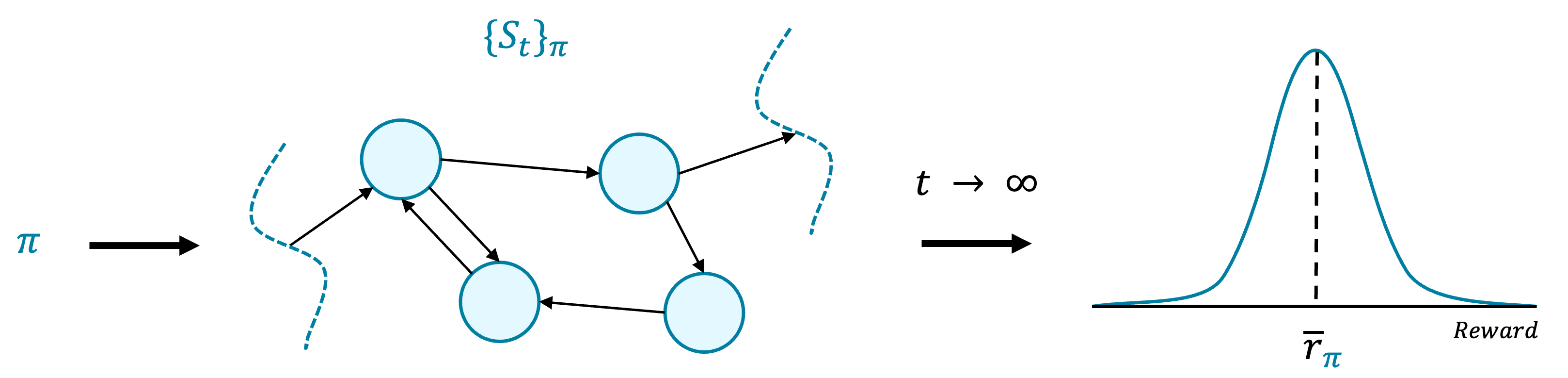
The underlying process by which average-reward MDPs operate is depicted in Fig. 1, where a given policy, $\pi$, induces a Markov chain, $\{S_{t}\}_{\pi}$, that yields a stationary reward distribution, whose mean corresponds to the long-run average-reward $\bar{r}_{\pi}$. Different policies can then be compared based on their $\bar{r}_{\pi}$ values to find the policy that yields the optimal average-reward.

In the context of RL, Wan et al. [8] proposed the tabular ‘Differential TD-learning’ and ‘Differential Q-learning’ algorithms, which approximate the state-value and state-action value functions as follows:

$\displaystyle V_{t+1}(S_{t})\doteq V_{t}(S_{t})+\alpha_{t}\rho_{t}\delta_{t}$ (6a)
$\displaystyle V_{t+1}(s)\doteq V_{t}(s),\quad\forall s\neq S_{t}$ (6b)
$\displaystyle\delta_{t}\doteq R_{t+1}-\bar{R}_{t}+V_{t}(S_{t+1})-V_{t}(S_{t})$ (6c)
$\displaystyle\bar{R}_{t+1}\doteq\bar{R}_{t}+\eta\alpha_{t}\rho_{t}\delta_{t}$ (6d)
$\displaystyle Q_{t+1}(S_{t},A_{t})\doteq Q_{t}(S_{t},A_{t})+\alpha_{t}\delta_{t}$ (7a)
$\displaystyle Q_{t+1}(s,a)\doteq Q_{t}(s,a),\quad\forall s,a\neq S_{t},A_{t}$ (7b)
$\displaystyle\delta_{t}\doteq R_{t+1}-\bar{R}_{t}+\max_{a}Q_{t}(S_{t+1},a)-Q_{t}(S_{t},A_{t})$ (7c)
$\displaystyle\bar{R}_{t+1}\doteq\bar{R}_{t}+\eta\alpha_{t}\delta_{t}$ (7d)

where, $\alpha_{t}$ is the step size, $\delta_{t}$ is the TD error, $\rho_{t}\doteq\pi(A_{t}\mid S_{t})\,/\,B(A_{t}\mid S_{t})$ is the importance sampling ratio (with behavior policy $B$), $\bar{R}_{t}$ is an estimate of the average-reward, $\bar{r}_{\pi}$, and $\eta$ is a positive scalar.

Refer to caption

Figure 1: Visual depiction of the underlying process by which average-reward MDPs operate. Here, following policy $\pi$ induces a Markov chain, ${\{S_{t}\}}_{\pi}$. As $t\to\infty$, this yields a stationary (or steady-state) reward distribution with an average reward, $\bar{r}_{\pi}$. It is this long-run (or steady-state) average-reward that the standard average-reward MDP formulation aims to optimize.

3.2 Conditional value-at-risk (CVaR)

Consider a random variable $X$ with a finite mean on a probability space $(\Omega,\mathcal{F},\mathbb{P})$, and with a cumulative distribution function $F(x)=\mathbb{P}(X\leq x)$. The (left-tail) value-at-risk (VaR) of $X$ with parameter $\tau\in(0,1)$ represents the $\tau$-quantile of $X$, such that $\text{VaR}_{\tau}(X)=\max\{x\mid F(x)\leq\tau\}$. The (left-tail) conditional value-at-risk (CVaR) of $X$ with parameter $\tau$ is defined as follows:

$$\text{CVaR}_{\tau}(X)=\frac{1}{\tau}\int_{0}^{\tau}\text{VaR}_{u}(X)du.$$ (8)

When $F(X)$ is continuous at $x=\text{VaR}_{\tau}(X)$, the conditional value-at-risk can be written as follows:

$$\text{CVaR}_{\tau}(X)=\mathbb{E}[X\mid X\leq\text{VaR}_{\tau}(X)].$$ (9)

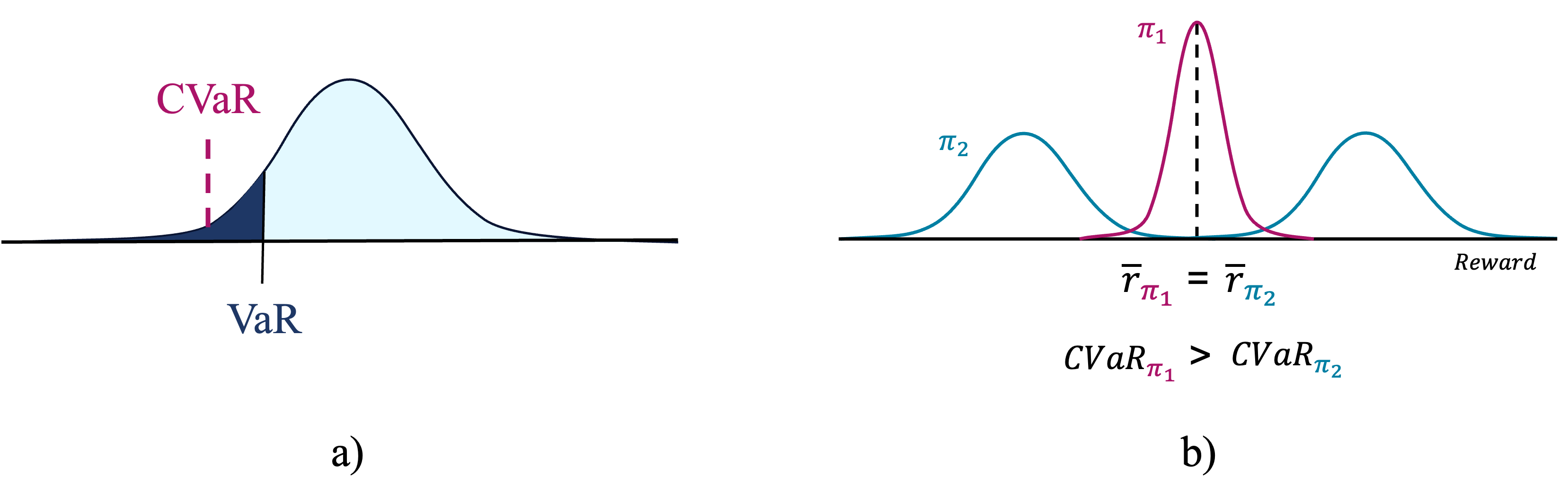
Hence, Equation (9) allows for the interpretation of CVaR as the expected value of the $\tau$ left quantile of the distribution of $X$. Fig. 2a) depicts this interpretation of CVaR. In this work, we aim to optimize the CVaR of the stationary reward distribution. Fig. 2b) compares the CVaR of two stationary reward distributions that have the same long-run average-reward. In recent years, CVaR has emerged as a popular risk measure, in-part because it is a ‘coherent’ risk measure [10], meaning that it satisfies key mathematical properties which can be meaningful in safety-critical and risk-related applications.

Refer to caption

Figure 2: a) The left-tail conditional value-at-risk (CVaR) of a probability distribution; b) The stationary reward distributions induced by two policies, $\pi_{1}$ and $\pi_{2}$. Both distributions have the same long-run average-reward, but different CVaR values.

An important, well-known property of CVaR, which we will use in our analysis, is that it can be represented as follows [5]:

$$\text{CVaR}_{\tau}(X)=\max_{b\in\mathbb{R}}\mathbb{E}[b-\frac{1}{\tau}(b-X)^{+}]=\mathbb{E}[\text{VaR}_{\tau}(X)-\frac{1}{\tau}(\text{VaR}_{\tau}(X)-X)^{+}],$$ (10)

where, $(y)^{+}=\max(y,0)$. Existing methods typically formulate the CVaR optimization problem as the following bi-level optimization with an augmented state-space that includes an estimate of $\text{VaR}_{\tau}(X)$ (in this case, $b$):

$$\max_{\pi}\text{CVaR}_{\tau}(X)=\max_{\pi}\max_{b\in\mathbb{R}}\mathbb{E}[b-\frac{1}{\tau}(b-X)^{+}]=\max_{b\in\mathbb{R}}(b-\frac{1}{\tau}\max_{\pi}\mathbb{E}[(b-X)^{+}]),$$ (11)

where the ‘inner’ optimization problem can be solved using standard MDP solution methods.

4 Reward-extended differential (RED) reinforcement learning

We now present our primary contribution: a framework for solving various subtasks simultaneously in the average-reward setting. We call this framework reward-extended differential (or RED) reinforcement learning. The ‘differential’ part of the name comes from the use of the differential algorithms from average-reward MDPs. The ‘reward-extended’ part of the name comes from the use of the reward-extended TD error, a novel concept that we will introduce shortly. We will show how combining the reward-extended TD error with a unique structural property of average-reward MDPs allows us to solve various subtasks simultaneously in an effective and efficient manner. We first derive the overall framework, then present a family of RL algorithms that utilize the framework. In the subsequent section, we will utilize this framework to tackle the CVaR optimization problem.

4.1 The framework

We begin our discussion by first describing what is meant by a ‘subtask’. Consider our goal of finding a policy that induces a stationary reward distribution with an optimal reward CVaR. We can see from Equation (10) that the reward CVaR can be interpreted as an expectation (or average) of sorts, which suggests that it may be possible to leverage the average-reward MDP to optimize this expectation, by treating the reward CVaR as the $\bar{r}_{\pi}$ that we want to optimize. However, this requires that we know the optimal value of the scalar $b$, because the aforementioned expectation only holds for this optimal value (which corresponds to the reward VaR, as per Equation (10)). Unfortunately, this optimal value is typically not known beforehand, so in order to optimize CVaR, we also need to optimize $b$. In this scenario, $b$ is the subtask that we are interested in solving because if we optimize $b$, in addition to CVaR, we will have our desired optimal solution. More generally, we can define a subtask as follows:

Definition 4.1 (Subtask).

A subtask, $z_{i}$, is any scalar prediction or control objective belonging to a corresponding finite set $\mathcal{Z}_{i}\subset\mathbb{R}$, such that:

i) there exists a linear (or piecewise linear) function, $f:\mathcal{R}\,\times\,\mathcal{Z}_{1}\,\times\,\mathcal{Z}_{2}\,\times\,\cdots\,\times\,\mathcal{Z}_{i}\,\times\,\cdots\,\times\,\mathcal{Z}_{n}\rightarrow\tilde{\mathcal{R}}$, that is invertible with respect to each input given all other inputs, where $\mathcal{R}$ is the finite set of observed per-step rewards from the MDP $\mathcal{M}$, $\mathcal{\tilde{R}}\subset\mathbb{R}$ is a modified, finite set of per-step rewards whose long-run average is the primary prediction or control objective of the modified MDP, $\mathcal{\tilde{M}}\doteq\langle\mathcal{S},\mathcal{A},\mathcal{\tilde{R}},p\rangle$, and $\mathcal{Z}=\{z_{1}\in\mathcal{Z}_{1},z_{2}\in\mathcal{Z}_{2},\ldots,z_{n}\in\mathcal{Z}_{n}\}$ is the set of $n$ subtasks that we wish to solve; and

ii) $z_{i}$ is independent of the states and actions, and hence independent of the observed per-step reward, $r\in\mathcal{R}$, such that $\mathbb{E}[f(r,z_{1},z_{2},\ldots,z_{n})]=f(\mathbb{E}[r],z_{1},z_{2},\ldots,z_{n})$.

With this definition in mind, we now proceed by providing the basic intuition behind our framework by using the average-reward itself, $\bar{r}_{\pi}$, as a blueprint of sorts for how we will derive the update rules in our learning algorithms for our subtasks. In particular, we will show how the process for deriving the update rule for the average-reward estimate, $\bar{R}_{t}$, in Equations (6) and (7) can be adapted to derive equivalent update rules for estimates corresponding to any subtask that satisfies Definition 4.1.

Consider the Bellman equation (4). We begin by pointing out that the average-reward satisfies many of the key properties of a subtask. In particular, we can see that $\bar{r}_{\pi}$ satisfies $\mathbb{E}[r-\bar{r}_{\pi}+v_{\pi}(s^{\prime})]=\mathbb{E}[r+v_{\pi}(s^{\prime})]-\bar{r}_{\pi}$. This allows us to rewrite the Bellman equation (4) as follows:

$$\bar{r}_{\pi}=\sum_{a}\pi(a\mid s)\sum_{s^{\prime},r}p(s^{\prime},r\mid s,a)[r+v_{\pi}(s^{\prime})-v_{\pi}(s)].$$ (12)

Now, if we wanted to learn $\bar{r}_{\pi}$ from experience, we can utilize the common RL update rule of the form: NewEstimate $\leftarrow$ OldEstimate $+$ StepSize [Target $-$ OldEstimate] [2] to do so. In this case, the ‘target’ is the term inside the expectation in Equation (12). This yields the update in Equation (6d): $\bar{R}_{t+1}=\bar{R}_{t}+\eta\alpha\delta_{t}$. Hence, we are able to learn $\bar{r}_{\pi}$ using the TD error, $\delta$. This highlights a unique structural property of average-reward MDPs: we are able to simultaneously predict (learn) the value function and the average-reward using the TD error. Similarly, in the control case we are able to simultaneously control (optimize) these same two objectives using the TD error.

We will now show, through the RED RL framework, how this structural property can be utilized to simultaneously predict or control any subtask that satisfies Definition 4.1. More specifically, we will show how we can replicate what we just did for the average-reward for any arbitrary subtask:

Theorem 4.1 (The RED Theorem).

An average-reward MDP can simultaneously predict or control any arbitrary number of subtasks using the TD error.

Proof.

Let $\tilde{r}=f(r,z_{1},z_{2},\ldots,z_{n})=f(\cdot)$ be a valid subtask function (as per Definition 4.1) corresponding to $n$ subtasks, where $r\in\mathcal{R}$ is the observed per-step reward, and $\tilde{r}\in\mathcal{\tilde{R}}$ is the modified per-step reward whose long-run average, $\bar{r}_{\pi}$, is the primary prediction or control objective.

First consider the TD error for the prediction case: $\delta=\tilde{r}-\bar{r}_{\pi}+v_{\pi}(s^{\prime})-v_{\pi}(s)=f(r,z_{1},z_{2},\ldots,z_{n})-\bar{r}_{\pi}+v_{\pi}(s^{\prime})-v_{\pi}(s)$. Because the TD error is a linear function of $\tilde{r}=f(\cdot)$, and because $f(\cdot)$ itself is linear and satisfies $\mathbb{E}[f(r,z_{1},\ldots,z_{n})]=f(\mathbb{E}[r],z_{1},\ldots,z_{n})$, we have, by linearity of expectation:

$\displaystyle\mathbb{E}[\delta]$ $\displaystyle=\mathbb{E}[f(r,z_{1},z_{2},\ldots,z_{n})-\bar{r}_{\pi}+v_{\pi}(s^{\prime})-v_{\pi}(s)]$ (13a)
$\displaystyle=f(\mathbb{E}[r-\bar{r}_{\pi}+v_{\pi}(s^{\prime})-v_{\pi}(s)],z_{1},\ldots,z_{n}).$ (13b)

Now consider an arbitrary subtask, $z_{i}\in\mathcal{Z}_{i}$, in Equation (13b). Since $f(\cdot)$ is linear and invertible with respect to each input given all other inputs, we can write $z_{i}$ as follows:

$\displaystyle z_{i}$ $\displaystyle=f^{-1}(\mathbb{E}[\delta]\mid\mathbb{E}[r-\bar{r}_{\pi}+v_{\pi}(s^{\prime})-v_{\pi}(s)],z_{1},\ldots,z_{i-1},z_{i+1},\ldots,z_{n}))$ (14a)
$\displaystyle z_{i}$ $\displaystyle=\mathbb{E}[f^{-1}(\delta\mid r-\bar{r}_{\pi}+v_{\pi}(s^{\prime})-v_{\pi}(s),z_{1},\ldots,z_{i-1},z_{i+1},\ldots,z_{n})]$ (14b)
$\displaystyle\doteq\mathbb{E}[f^{-1}_{i}(\delta)],$ (14c)

where $f^{-1}_{i}(\delta)$ denotes the inverse of the TD error with respect to $z_{i}$ given all other inputs.

Now, let $g_{z_{i}}$ denote $f^{-1}_{i}(\delta)$ when $\delta=0$, such that $g_{z_{i}}\doteq f^{-1}_{i}(0)$. With this notation in mind, and denoting the expectation, $\mathbb{E}$, as shorthand for the sums in the Bellman equation (4), we can rewrite the Bellman equation (4) for the MDP $\mathcal{\tilde{M}}$ and solve for $z_{i}$ as follows:

$\displaystyle v_{\pi}(s)$ $\displaystyle=\mathbb{E}[f(r,z_{1},z_{2},\ldots,z_{n})-\bar{r}_{\pi}+v_{\pi}(s^{\prime})]$ (15a)
$\displaystyle 0$ $\displaystyle=\mathbb{E}[f(r,z_{1},z_{2},\ldots,z_{n})-\bar{r}_{\pi}+v_{\pi}(s^{\prime})-v_{\pi}(s)]$ (15b)
$\displaystyle 0$ $\displaystyle=f\left(\mathbb{E}[r-\bar{r}_{\pi}+v_{\pi}(s^{\prime})-v_{\pi}(s)],z_{1},z_{2},\ldots,z_{n}\right)$ (15c)
$\displaystyle z_{i}$ $\displaystyle=\mathbb{E}[f^{-1}_{i}(0)]$ (15d)
$\displaystyle z_{i}$ $\displaystyle=\mathbb{E}[g_{z_{i}}].$ (15e)

Thus, to learn $z_{i}$ from experience, we can utilize the common RL update rule (in a similar fashion to what we did with Equation (12) for the average-reward), which yields the update:

$\displaystyle Z_{i,t+1}$ $\displaystyle=Z_{i,t}+\eta\alpha[g_{{z_{i}},t}-Z_{i,t}]$ (16a)
$\displaystyle\doteq Z_{i,t}+\eta\alpha\beta_{i,t},$ (16b)

where $Z_{i,t}$ is the estimate of subtask $z_{i}$ at time $t$, and $\eta\alpha$ is the step size.

Here, we define $\beta_{i}$ as the reward-extended TD error for subtask $z_{i}$. Our rationale for the naming of the reward-extended TD error stems from the fact that this term satisfies a TD error-dependent property: it goes to zero as the TD error, $\delta$, goes to zero. This follows from Equation (15e), where $g_{z_{i}}=z_{i}$ when $\delta=0$, which consequently zeroes out the reward-extended TD error in Equation (16). This implies that, like the average-reward update in Equation (6d), the arbitrary subtask update is dependent on the TD error, such that the subtask estimate will only cease to update once the TD error is zero. Hence, minimizing the TD error allows us to solve the arbitrary subtask simultaneously. This relationship between the reward-extended TD error and the regular TD error is formalized in Corollary 4.1 below. In Section 5, we will see that this property allows us to write the reward-extended TD error update as some constant, subtask-specific fraction of the regular TD error update.

Corollary 4.1.

Let $\beta_{i,t}$ denote the reward-extended TD error for subtask $z_{i}$, and $\delta_{t}$ denote the regular TD error at time $t$. Then, $\beta_{i,t}=0$ if $\delta_{t}=0$.

Proof.

Consider the definition of the reward-extended TD error, $\beta_{i,t}\doteq g_{{z_{i}},t}-Z_{i,t}$. By Equation (15), when $\delta_{t}=0$, then $g_{{z_{i}},t}=Z_{i,t}$. As such, $\beta_{i,t}=0$ when $\delta_{t}=0$. ∎

As such, we have derived an update rule based on the TD error for our arbitrary subtask, $z_{i}$. Finally, because we picked $z_{i}$ arbitrarily, it follows that we can derive an update rule for every subtask in $f(\cdot)$ based on the TD error. This means that we can perform prediction for all our subtasks simultaneously by minimizing the (regular) TD error. The same logic can be applied in the control case to derive equivalent updates, where we note that it directly follows from Definition 4.1 that the existence of an optimal average-reward, $\bar{r}*$, implies the existence of corresponding optimal subtask values, $z_{i}^{*}\;\forall z_{i}\in\mathcal{Z}$. This completes the proof of Theorem 4.1. ∎

4.2 The algorithms

We now present our family of RED RL algorithms. The full set of algorithms, including algorithms that utilize function approximation, are included in Appendix A. We provide full convergence proofs for the tabular algorithms in Appendix B.

RED TD-learning algorithm (tabular): We update a table of estimates, $V_{t}:\mathcal{S}\rightarrow\mathbb{R}$ as follows:

$\displaystyle\tilde{R}_{t+1}=f(R_{t+1},Z_{1,t},Z_{2,t},\ldots,Z_{n,t})$ (17a)
$\displaystyle\delta_{t}=\tilde{R}_{t+1}-\bar{R}_{t}+V_{t}(S_{t+1})-V_{t}(S_{t})$ (17b)
$\displaystyle V_{t+1}(S_{t})=V_{t}(S_{t})+\alpha_{t}\rho_{t}\delta_{t}$ (17c)
$\displaystyle V_{t+1}(s)=V_{t}(s),\quad\forall s\neq S_{t}$ (17d)
$\displaystyle\bar{R}_{t+1}=\bar{R}_{t}+\eta_{r}\alpha_{t}\rho_{t}\delta_{t}$ (17e)
$\displaystyle Z_{i,t+1}=Z_{i,t}+\eta_{z_{i}}\alpha_{t}\rho_{t}\beta_{i,t},\quad\forall z_{i}\in\mathcal{Z}$ (17f)

where, $R_{t}$ is the observed reward, $Z_{i,t}$ is an estimate of subtask $z_{i}$, $\beta_{i,t}$ is the reward-extended TD error for subtask $z_{i}$, $\alpha_{t}$ is the step size, $\delta_{t}$ is the TD error, $\rho_{t}$ is the importance sampling ratio, $\bar{R}_{t}$ is an estimate of the long-run average-reward of $\tilde{R}_{t}$, $\bar{r}_{\pi}$, and $\eta_{r},\eta_{z_{i}}$ are positive scalars. Wan et al. [8] showed for their Differential TD-learning algorithm that $R_{t}$ converges to $\bar{r}_{\pi}$, and $V_{t}$ converges to a solution of $v$ in Equation (4) for a given policy $\pi$. We now provide an equivalent theorem for our RED TD-learning algorithm, which also shows that $Z_{i,t}$ converges to $z_{i,{\pi}}\;\forall z_{i}\in\mathcal{Z}$, where $z_{i,{\pi}}$ denotes the subtask value when following policy $\pi$:

Theorem 4.2 (informal).

The RED TD-learning algorithm (17) converges, almost surely, $\bar{R}_{t}$ to $\bar{r}_{\pi}$, $Z_{i,t}$ to $z_{i,{\pi}}\;\forall z_{i}\in\mathcal{Z}$, and $V_{t}$ to a solution of $v$ in the Bellman Equation (4), if the following assumptions hold: 1) the Markov chain induced by the target policy $\pi$ is unichain, 2) every state–action pair for which $\pi(a\mid s)>0$ occurs an infinite number of times under the behavior policy, 3) the step sizes are decreased appropriately, 4) the ratio of the update frequency of the most-updated state to the least-updated state is finite, and 5) the subtasks are in accordance with Definition 4.1.

Proof.

See Appendix B for the full proof. ∎

RED Q-learning algorithm (tabular): We update a table of estimates, $Q_{t}:\mathcal{S}\,\times\,\mathcal{A}\rightarrow\mathbb{R}$ as follows:

$\displaystyle\tilde{R}_{t+1}=f(R_{t+1},Z_{1,t},Z_{2,t},\ldots,Z_{n,t})$ (18a)
$\displaystyle\delta_{t}=\tilde{R}_{t+1}-\bar{R}_{t}+\max_{a}Q_{t}(S_{t+1},a)-Q_{t}(S_{t},A_{t})$ (18b)
$\displaystyle Q_{t+1}(S_{t},A_{t})=Q_{t}(S_{t},A_{t})+\alpha_{t}\delta_{t}$ (18c)
$\displaystyle Q_{t+1}(s,a)=Q_{t}(s,a),\quad\forall s,a\neq S_{t},A_{t}$ (18d)
$\displaystyle\bar{R}_{t+1}=\bar{R}_{t}+\eta_{r}\alpha_{t}\delta_{t}$ (18e)
$\displaystyle Z_{i,t+1}=Z_{i,t}+\eta_{z_{i}}\alpha_{t}\beta_{i,t},\quad\forall z_{i}\in\mathcal{Z}$ (18f)

where, $R_{t}$ is the observed reward, $Z_{i,t}$ is an estimate of subtask $z_{i}$, $\beta_{i,t}$ is the reward-extended TD error for subtask $z_{i}$, $\alpha_{t}$ is the step size, $\delta_{t}$ is the TD error, $\bar{R}_{t}$ is an estimate of the long-run average-reward of $\tilde{R}_{t}$, $\bar{r}_{\pi}$, and $\eta_{r},\eta_{z_{i}}$ are positive scalars. Wan et al. [8] showed for their Differential Q-learning algorithm that $R_{t}$ converges to $\bar{r}*$, and $Q_{t}$ converges to a solution of $q$ in Equation (5). We now provide an equivalent theorem for our RED Q-learning algorithm, which also shows that $Z_{i,t}$ converges to the corresponding optimal subtask value $z_{i}^{*}\;\forall z_{i}\in\mathcal{Z}$:

Theorem 4.3 (informal).

The RED Q-learning algorithm (18) converges, almost surely, $\bar{R}_{t}$ to $\bar{r}*$, $Z_{i,t}$ to $z_{i}^{*}\;\forall z_{i}\in\mathcal{Z}$, $Q_{t}$ to a solution of $q$ in the Bellman Equation (5), $\bar{r}_{\pi_{t}}$ to $\bar{r}*$, and $z_{i,{\pi_{t}}}$ to $z_{i}^{*}\;\forall z_{i}\in\mathcal{Z}$, for all $s\in\mathcal{S}$, where $\pi_{t}$ is any greedy policy with respect to $Q_{t}$, if the following assumptions hold: 1) the MDP is communicating, 2) the solution of $q$ in 5 is unique up to a constant, 3) the step sizes are decreased appropriately, 4) all the state–action pairs are updated an infinite number of times, 5) the ratio of the update frequency of the most-updated state–action pair to the least-updated state–action pair is finite, and 6) the subtasks are in accordance with Definition 4.1.

Proof.

See Appendix B for the full proof. ∎

5 Case study: RED RL for CVaR optimization

We now illustrate the usefulness of the RED RL framework by showing how it can be used to learn a policy that optimizes the CVaR risk measure without the use of an explicit bi-level optimization scheme (as in Equation (11)), or an augmented state-space.

As mentioned in Section 4.1, our goal is to learn a policy that induces a stationary reward distribution with an optimal reward CVaR (instead of the regular average-reward). Here, the reward CVaR is our primary control objective (i.e., the $\bar{r}_{\pi}$ that we want to optimize), and the reward VaR ($b$ in Equation (10)) is our subtask. When we apply the RED RL framework, using a modified version of Equation (10) as the subtask function (see Appendix C for more details), we arrive at the RED CVaR algorithms (see Appendix C for the full algorithms), which have the following update for our subtask, VaR:

$$\text{VaR}_{t+1}=\begin{cases}\text{VaR}_{t}-\eta\alpha\delta_{t},&R_{t}\geq\text{VaR}_{t}\\ \text{VaR}_{t}+\eta\alpha(\frac{\tau}{1-\tau})\delta_{t}&R_{t}<\text{VaR}_{t}\end{cases}\,,$$ (19)

where $\eta\alpha$ is the step size, $\tau$ is the CVaR parameter, and $\delta_{t}$ is the regular TD error. As such, we can see that a subtask update, which utilizes the reward-extended TD error, ultimately amounts to an ‘extended’ version of the regular TD update. Consequently, this update rule allows us to optimize our subtask, VaR, without the use of an explicit bi-level optimization scheme or an augmented state-space.

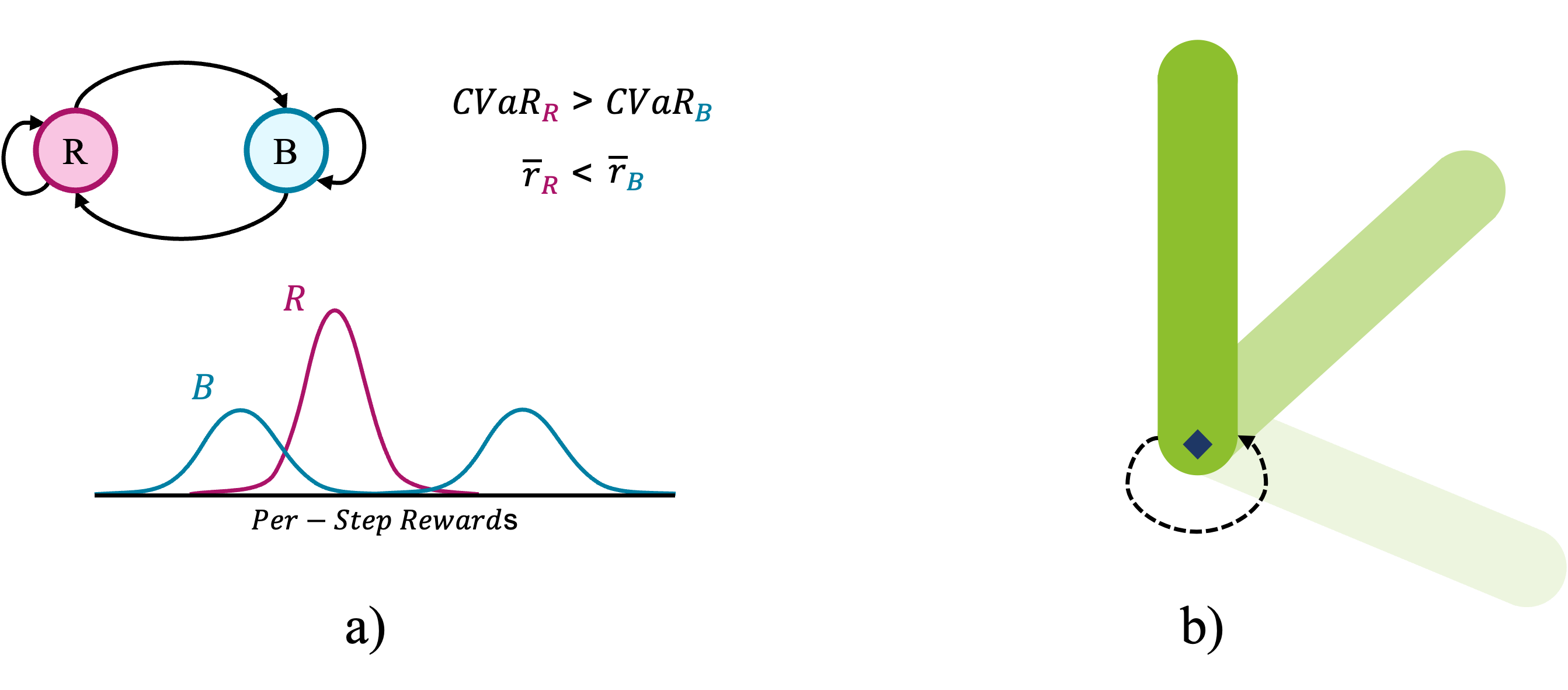
We now present empirical results when applying the RED CVaR algorithms on two learning tasks. The first task is a two-state environment that we created for the purposes of testing our algorithms. It is called the red-pill blue-pill environment (see Appendix D), where at every time step an agent can take either a red pill, which takes them to the ‘red world’ state, or a blue pill, which takes them to the ‘blue world’ state. Each state has its own characteristic reward distribution, and in this case, the red world state has a reward distribution with a lower (worse) mean but higher (better) CVaR compared to the blue world state. Hence, we would expect the regular Differential Q-learning algorithm to learn a policy that prefers to stay in the blue world, and that the RED CVaR Q-learning algorithm learns a policy that prefers to stay in the red world. This task is illustrated in Fig. 3a).

The second learning task is the well-known inverted pendulum task, where an agent learns how to optimally balance an inverted pendulum. We chose this task because it provides us with opportunity to test our algorithm in an environment where: 1) we must use function approximation (given the large state and action spaces), and 2) where the policy for the optimal average-reward and the policy for the optimal reward CVaR is the same policy (i.e., the policy that best balances the pendulum will yield a stationary reward distribution with both the optimal average-reward and reward CVaR). This hence allows us to directly compare the performance of our RED algorithms to the regular Differential learning algorithms, as well as to gauge how function approximation affects the performance of our algorithms. For this task, we utilized a simple actor-critic architecture [2] as this allowed us to compare the performance of the (non-tabular) RED TD-learning algorithm with a (non-tabular) Differential TD-learning algorithm. This task is illustrated in Fig. 3b). The full set of experimental details, including the full algorithms used, can be found in Appendix C.

Refer to caption

Figure 3: An illustration of the a) red-pill blue-pill, and b) inverted pendulum environments.

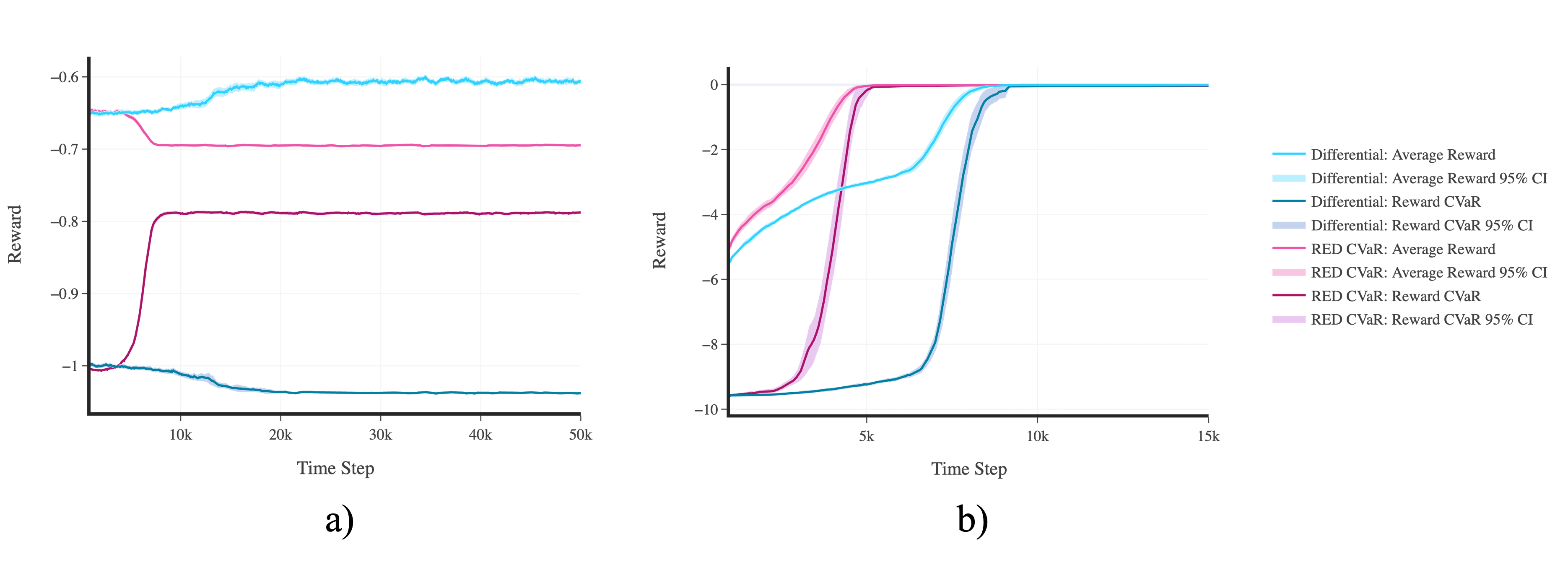
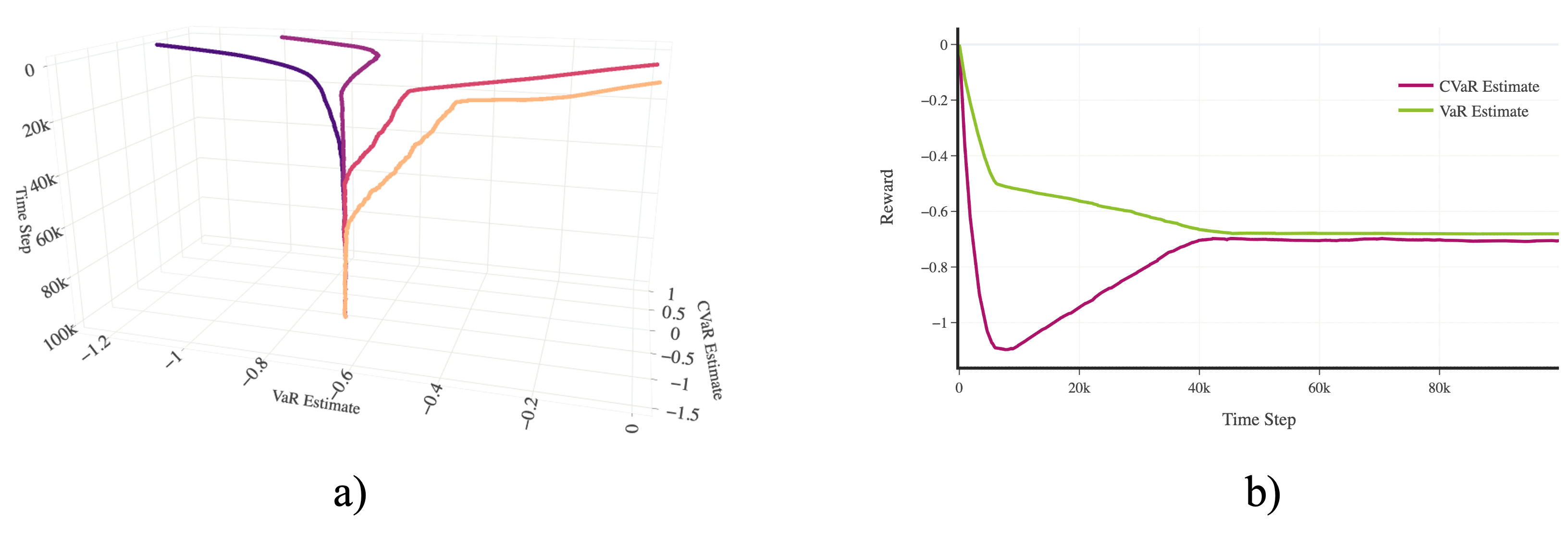
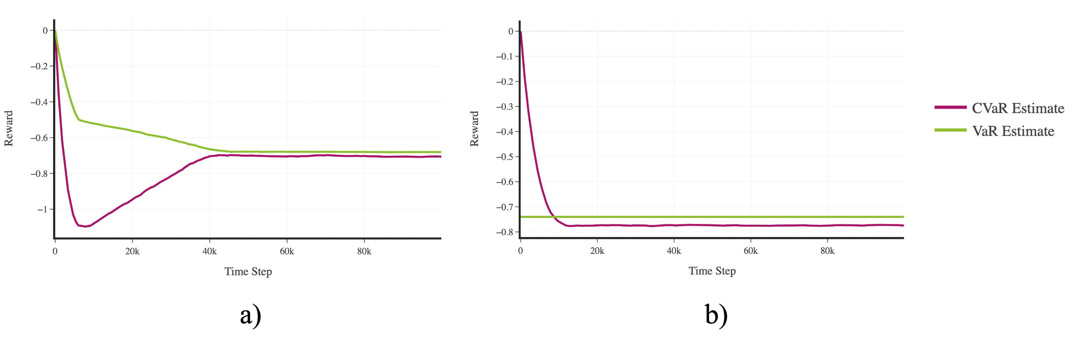
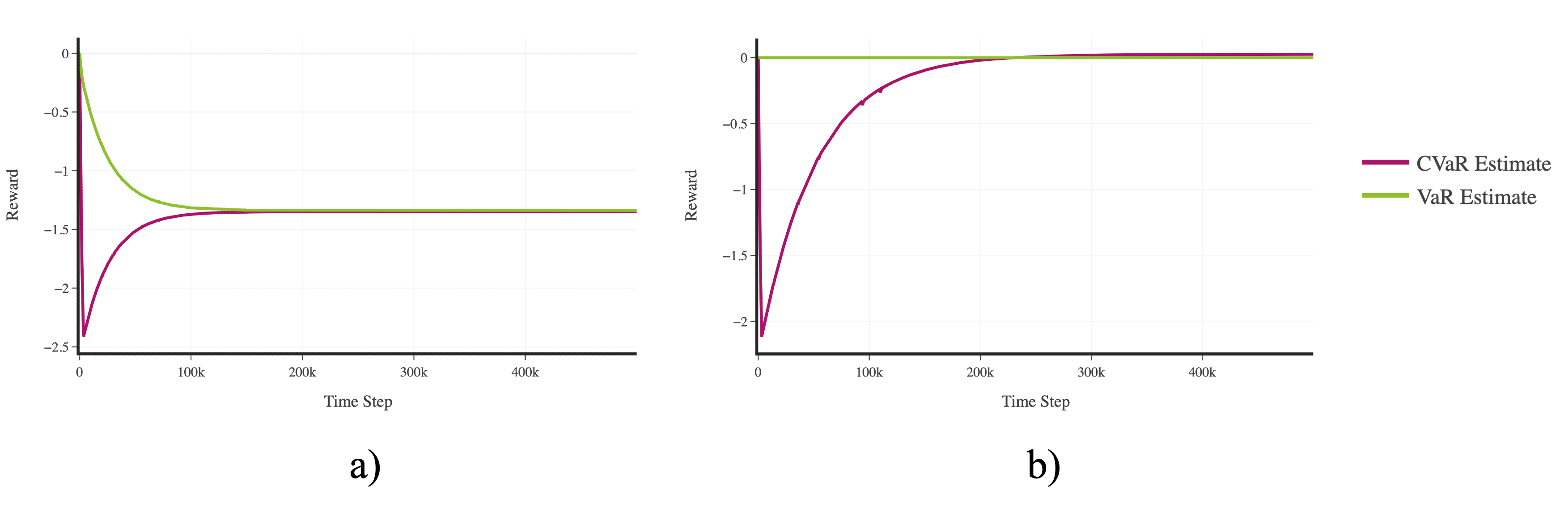
In terms of empirical results, Fig. 4 shows rolling averages of the average-reward and reward CVaR as learning progresses in both tasks when using the regular Differential learning algorithms (to optimize the average-reward) vs. the RED CVaR learning algorithms (to optimize the reward CVaR). As shown in the figure, in the red-pill blue-pill task the RED CVaR algorithm is able to successfully learn a policy that prioritizes maximizing the reward CVaR over the average-reward, thereby achieving a sort of risk-awareness. In the inverted pendulum task, both methods converge to the same policy, as expected. Fig. 5 shows typical convergence plots of the agent’s VaR and CVaR estimates as learning progresses on the red-pill blue-pill task for various combinations of initial VaR and CVaR guesses. We see that regardless of the initial guess, the estimates still converge. These estimates converge to the correct VaR and CVaR values, up to a constant, thereby yielding the optimal CVaR policy, as in Fig. 4a). See Appendix C for a more detailed discussion of the empirical results.

Refer to caption

Figure 4: Rolling average-reward and reward CVaR as learning progresses when using the (risk-neutral) Differential algorithms vs. the (risk-aware) RED CVaR algorithms in the a) red-pill blue-pill, and b) inverted pendulum tasks. A solid line denotes the mean average-reward or reward CVaR, and the corresponding shaded region denotes the 95% confidence interval over 50 runs.

Refer to caption

Figure 5: Convergence plots of the agent’s VaR and CVaR estimates as learning progresses when using the RED CVaR Q-learning algorithm on the red-pill blue-pill task with a) various combinations of initial VaR and CVaR guesses, and b) an initial guess of 0.0 for both the VaR and CVaR estimates.

6 Discussion, limitations, and future work

In this work, we introduced reward-extended differential (or RED) reinforcement learning: a novel reinforcement learning framework that can be used to solve various subtasks simultaneously in the average-reward setting. We introduced a family of RED RL algorithms for prediction and control, and then showcased how these algorithms could be adopted to effectively and efficiently tackle the CVaR optimization problem. More specifically, we were able to use the RED RL framework to successfully learn a policy that optimized the CVaR risk measure without using an explicit bi-level optimization scheme or an augmented state-space, thereby alleviating some of the computational challenges and non-trivialities that arise when performing risk-based optimization in the episodic and discounted settings. Empirically, we showed that the RED-based CVaR algorithms fared well both in tabular and linear function approximation settings. Moreover, our experiments suggest that these algorithms are robust to the initial guesses for the subtasks and primary learning objective.

More broadly, our work has introduced a theoretically-sound framework that allows for a subtask-driven approach to reinforcement learning, where various learning problems (or subtasks) are solved simultaneously to help solve a larger, central learning problem. In this work, we showed (both theoretically and empirically) how this framework can be utilized to predict and/or optimize any arbitrary number of subtasks simultaneously in the average-reward setting. Central to this result is the novel concept of the reward-extended TD error, which is utilized in our framework to develop learning rules for the subtasks, and satisfies key theoretical properties that make it possible to solve any given subtask in a fully-online manner by minimizing the regular TD error. Moreover, we built-upon existing results from Wan et al. [8] to show the almost sure convergence of tabular algorithms derived from our framework. While we have only begun to grasp the implications of our framework, we have already seen some promising indications in the CVaR case study: the ability to turn explicit bi-level optimization problems into implicit bi-level optimizations that can be solved in a fully-online manner, as well as the potential to turn certain states (that meet certain conditions) into subtasks, thereby reducing the size of the state-space.

Nonetheless, while these results are encouraging, they are subject to a number of limitations. Firstly, by nature of operating in the average-reward setting, we are subject to the somewhat-strict assumptions made about the Markov chain induced by the policy (e.g. unichain or communicating). These assumptions could restrict the applicability of our framework, as they may not always hold in practice. Similarly, our definition for a subtask requires that the associated subtask function be linear, which may also limit the applicability of our framework to simpler functions. Finally, it remains to be seen empirically how our framework performs when dealing with multiple subtasks, when taking on more complex tasks, and/or when utilizing nonlinear function approximation.

In future work, we hope to address many of these limitations, as well as explore how these promising results can be extended to other domains, beyond the risk-awareness problem. In particular, we believe that the ability to optimize various subtasks simultaneously, as well as the potential to reduce the size of the state-space, by converting certain states to subtasks (where appropriate), could help alleviate significant computational challenges in other areas moving forward.

Acknowledgments and Disclosure of Funding

The authors would like to thank Margaret P. Chapman for insightful conversations and feedback in the early stages of this work.

References

  • [1] M. L. Puterman, Markov Decision Processes: Discrete Stochastic Dynamic Programming. John Wiley & Sons, 1994.
  • [2] R. S. Sutton and A. G. Barto, Reinforcement Learning, second edition: An Introduction. MIT Press, Nov. 2018.
  • [3] G. Dulac-Arnold, N. Levine, D. J. Mankowitz, J. Li, C. Paduraru, S. Gowal, and T. Hester, “Challenges of real-world reinforcement learning: definitions, benchmarks and analysis,” Mach. Learn., vol. 110, pp. 2419–2468, Sept. 2021.
  • [4] R. S. Sutton, “Learning to predict by the methods of temporal differences,” Mach. Learn., vol. 3, p. 944, 1988.
  • [5] R. T. Rockafellar and S. Uryasev, “Optimization of conditional value-at-risk,” The Journal of Risk, vol. 2, no. 3, pp. 21–41, 2000.
  • [6] S. Mahadevan, “Average reward reinforcement learning: Foundations, algorithms, and empirical results,” Mach. Learn., vol. 22, no. 1-3, pp. 159–195, 1996.
  • [7] V. Dewanto, G. Dunn, A. Eshragh, M. Gallagher, and F. Roosta, “Average-reward model-free reinforcement learning: a systematic review and literature mapping,” arXiv [cs.LG], Oct. 2020.
  • [8] Y. Wan, A. Naik, and R. S. Sutton, “Learning and planning in average-reward markov decision processes,” in Proceedings of the 38th International Conference on Machine Learning, vol. 139 of Proceedings of Machine Learning Research, pp. 10653–10662, PMLR, 2021.
  • [9] R. A. Howard and J. E. Matheson, “Risk-sensitive markov decision processes,” Manage. Sci., vol. 18, pp. 356–369, Mar. 1972.
  • [10] P. Artzner, F. Delbaen, J.-M. Eber, and D. Heath, “Coherent measures of risk,” Math. Finance, vol. 9, pp. 203–228, July 1999.
  • [11] Y. Chow, A. Tamar, S. Mannor, and M. Pavone, “Risk-sensitive and robust decision-making: a CVaR optimization approach,” in Advances in neural information processing systems 28, 2015.
  • [12] S. H. Lim and I. Malik, “Distributional reinforcement learning for risk-sensitive policies,” in Advances in Neural Information Processing Systems 35 (NeurIPS 2022), 2022.
  • [13] Y. Wang and M. P. Chapman, “Risk-averse autonomous systems: A brief history and recent developments from the perspective of optimal control,” Artif. Intell., vol. 311, p. 103743, Oct. 2022.
  • [14] N. Bäuerle and A. Jaśkiewicz, “Markov decision processes with risk-sensitive criteria: an overview,” Mathematical Methods of Operations Research, Apr. 2024.
  • [15] L. Xia, L. Zhang, and P. W. Glynn, “Risk-sensitive markov decision processes with long-run CVaR criterion,” Prod. Oper. Manag., vol. 32, pp. 4049–4067, Dec. 2023.
  • [16] V. S. Borkar, “Asynchronous stochastic approximations,” SIAM Journal on Control snd Optimization, vol. 36, no. 3, pp. 840–851, 1998.
  • [17] J. Abounadi, D. Bertsekas, and V. S. Borkar, “Learning algorithms for markov decision processes with average cost,” SIAM Journal on Control and Optimization, vol. 40, no. 3, pp. 681–698, 2001.
  • [18] D. Bertsekas and J. N. Tsitsiklis, Neuro-Dynamic Programming. Athena Scientific, 1996.
  • [19] M. G. Bellemare, W. Dabney, and M. Rowland, Distributional reinforcement learning. The MIT Press, 2023.

Appendix A RED RL algorithms

In this Appendix, we provide pseudocode for our RED RL algorithms. We first present tabular algorithms, whose convergence proofs are included in Appendix B, and then provide equivalent algorithms that utilize function approximation.

Algorithm 1 RED TD-Learning (Tabular)
  Input: the policy $\pi$ to be evaluated, policy $B$ to be used, subtask function $f$, inverse functions $g_{z_{1}},g_{z_{2}},\ldots,g_{z_{n}}$
  Algorithm parameters: step size parameters $\alpha$, $\eta_{r}$, $\eta_{z_{1}},\eta_{z_{2}},\ldots,\eta_{z_{n}}$
  Initialize $V(s)\>\forall s;\bar{R}$ arbitrarily (e.g. to zero)
  Initialize subtasks $Z_{1},Z_{2},\ldots,Z_{n}$ arbitrarily (e.g. to zero)
  Obtain initial $S$
  while still time to train do
     $A\leftarrow$ action given by $B$ for $S$
     Take action $A$, observe $R,S^{\prime}$
     $\tilde{R}=f(R,Z_{1},Z_{2},\ldots,Z_{n})$
     $\delta=\tilde{R}-\bar{R}+V(S^{\prime})-V(S)$
     $\rho=\pi(A\mid S)/B(A\mid S)$
     $V(S)=V(S)+\alpha\rho\delta$
     $\bar{R}=\bar{R}+\eta_{r}\alpha\rho\delta$
     $\beta_{i}=g_{z_{i}}-Z_{i},\quad\forall i=1,2,\ldots,n$
     $Z_{i}=Z_{i}+\eta_{z_{i}}\alpha\rho\beta_{i},\quad\forall i=1,2,\ldots,n$
     $S=S^{\prime}$
  end while
  return V
Algorithm 2 RED Q-Learning (Tabular)
  Input: the policy $\pi$ to be used (e.g., $\epsilon$-greedy), subtask function $f$, inverse functions $g_{z_{1}},g_{z_{2}},\ldots,g_{z_{n}}$
  Algorithm parameters: step size parameters $\alpha$, $\eta_{r}$, $\eta_{z_{1}},\eta_{z_{2}},\ldots,\eta_{z_{n}}$
  Initialize $Q(s,a)\>\forall s,a;\bar{R}$ arbitrarily (e.g. to zero)
  Initialize subtasks $Z_{1},Z_{2},\ldots,Z_{n}$ arbitrarily (e.g. to zero)
  Obtain initial $S$
  while still time to train do
     $A\leftarrow$ action given by $\pi$ for $S$
     Take action $A$, observe $R,S^{\prime}$
     $\tilde{R}=f(R,Z_{1},Z_{2},\ldots,Z_{n})$
     $\delta=\tilde{R}-\bar{R}+\max_{a}Q(S^{\prime},a)-Q(S,A)$
     $Q(S,A)=Q(S,A)+\alpha\delta$
     $\bar{R}=\bar{R}+\eta_{r}\alpha\delta$
     $\beta_{i}=g_{z_{i}}-Z_{i},\quad\forall i=1,2,\ldots,n$
     $Z_{i}=Z_{i}+\eta_{z_{i}}\alpha\beta_{i},\quad\forall i=1,2,\ldots,n$
     $S=S^{\prime}$
  end while
  return Q
Algorithm 3 RED TD-Learning (Function Approximation)
  Input: the policy $\pi$ to be evaluated, policy $B$ to be used, a differentiable state-value function parameterization: $\hat{v}(s,\boldsymbol{w})$, subtask function $f$, inverse functions $g_{z_{1}},g_{z_{2}},\ldots,g_{z_{n}}$
  Algorithm parameters: step size parameters $\alpha$, $\eta_{r}$, $\eta_{z_{1}},\eta_{z_{2}},\ldots,\eta_{z_{n}}$
  Initialize state-value weights $\boldsymbol{w}\in\mathbb{R}^{d}$ arbitrarily (e.g. to $\boldsymbol{0}$)
  Initialize subtasks $Z_{1},Z_{2},\ldots,Z_{n}$ arbitrarily (e.g. to zero)
  Obtain initial $S$
  while still time to train do
     $A\leftarrow$ action given by $B$ for $S$
     Take action $A$, observe $R,S^{\prime}$
     $\tilde{R}=f(R,Z_{1},Z_{2},\ldots,Z_{n})$
     $\delta=\tilde{R}-\bar{R}+\hat{v}(S^{\prime},\boldsymbol{w})-\hat{v}(S,\boldsymbol{w})$
     $\rho=\pi(A\mid S)/B(A\mid S)$
     $\boldsymbol{w}=\boldsymbol{w}+\alpha\rho\delta\nabla\hat{v}(S,\boldsymbol{w})$
     $\bar{R}=\bar{R}+\eta_{r}\alpha\rho\delta$
     $\beta_{i}=g_{z_{i}}-Z_{i},\quad\forall i=1,2,\ldots,n$
     $Z_{i}=Z_{i}+\eta_{z_{i}}\alpha\rho\beta_{i},\quad\forall i=1,2,\ldots,n$
     $S=S^{\prime}$
  end while
  return $\boldsymbol{w}$
Algorithm 4 RED Q-Learning (Function Approximation)
  Input: the policy $\pi$ to be used (e.g., $\epsilon$-greedy), a differentiable state-action value function parameterization: $\hat{q}(s,a,\boldsymbol{w})$, subtask function $f$, inverse functions $g_{z_{1}},g_{z_{2}},\ldots,g_{z_{n}}$
  Algorithm parameters: step size parameters $\alpha$, $\eta_{r}$, $\eta_{z_{1}},\eta_{z_{2}},\ldots,\eta_{z_{n}}$
  Initialize state-action value weights $\boldsymbol{w}\in\mathbb{R}^{d}$ arbitrarily (e.g. to $\boldsymbol{0}$)
  Initialize subtasks $Z_{1},Z_{2},\ldots,Z_{n}$ arbitrarily (e.g. to zero)
  Obtain initial $S$
  while still time to train do
     $A\leftarrow$ action given by $\pi$ for $S$
     Take action $A$, observe $R,S^{\prime}$
     $\tilde{R}=f(R,Z_{1},Z_{2},\ldots,Z_{n})$
     $\delta=\tilde{R}-\bar{R}+\max_{a}\hat{q}(S^{\prime},a,\boldsymbol{w})-\hat{q}(S,A,\boldsymbol{w})$
     $\boldsymbol{w}=\boldsymbol{w}+\alpha\delta\nabla\hat{q}(S,A,\boldsymbol{w})$
     $\bar{R}=\bar{R}+\eta_{r}\alpha\delta$
     $\beta_{i}=g_{z_{i}}-Z_{i},\quad\forall i=1,2,\ldots,n$
     $Z_{i}=Z_{i}+\eta_{z_{i}}\alpha\beta_{i},\quad\forall i=1,2,\ldots,n$
     $S=S^{\prime}$
  end while
  return $\boldsymbol{w}$

Appendix B Convergence proofs

In this Appendix, we present the full convergence proofs for the tabular RED TD-learning and tabular RED Q-learning algorithms. Our general strategy is as follows: we first show that the results from Wan et al. [8], which show the a.s. convergence of the value function and average-reward estimates of differential algorithms, are applicable to our algorithms. We then build upon these results to show that the subtask estimates of our algorithms converge as well.

For consistency, we adopt similar notation as Wan et al. [8] for our proofs:

  • For a given vector $x$, let $\sum x$ denote the sum of all elements in $x$, such that $\sum x\doteq\sum_{i}x(i)$.

  • Let $\bar{r}_{*}$ denote the optimal average-reward.

  • Let $z_{i_{*}}$ denote the corresponding optimal subtask value for subtask $z_{i}\in\mathcal{Z}$.

B.1 Convergence proof for the tabular RED TD-learning algorithm

In this section, we present the proof for the convergence of the value function, average-reward, and subtask estimates of the RED TD-learning algorithm. Similar to what was done in Wan et al. [8], we will begin by considering a general algorithm, called General RED TD. We will first define General RED TD, then show how the RED TD-learning algorithm is a special case of this algorithm. We will then provide necessary assumptions, state the convergence theorem of General RED TD, and then provide a proof for the theorem, where we show that the value function, average-reward, and subtask estimates converge, thereby showing that the RED TD-learning algorithm converges. We begin by introducing the General RED TD algorithm:

First consider an MDP $\mathcal{M}\doteq\langle\mathcal{S},\mathcal{A},\mathcal{R},p\rangle$, a behavior policy $B$, and a target policy $\pi$. Given a state $s\in\mathcal{S}$ and discrete step $n\geq 0$, let $A_{n}(s)\sim B(\cdot\mid s)$ denote the action selected using the behavior policy, let $R_{n}(s,A_{n}(s))\in\mathcal{R}$ denote a sample of the resulting reward, and let $S^{\prime}_{n}(s,A_{n}(s))\sim p(\cdot,\cdot\mid s,a)$ denote a sample of the resulting state. Let $\{Y_{n}\}$ be a set-valued process taking values in the set of nonempty subsets of $\mathcal{S}$, such that: $Y_{n}=\{s:s$ component of the $|\mathcal{S}|$-sized table of state-value estimates, $V$, that was updated at step $n\}$. Let $\nu(n,s)\doteq\sum_{j=0}^{n}I\{s\in Y_{j}\}$, where $I$ is the indicator function, such that $\nu(n,s)$ represents the number of times $V(s)$ was updated up to step $n$.

Now, let $f$ be a valid subtask function (see Definition 4.1), such that $\tilde{R}_{n}(s,A_{n}(s))\doteq f(R_{n}(s,A_{n}(s)),Z_{1,n},Z_{2,n},\ldots,Z_{k,n})$ for $k$ subtasks $\in\mathcal{Z}$, where $\mathcal{Z}$ is the set of subtasks, and $Z_{i,n}$ denotes the estimate of subtask $z_{i}\in\mathcal{Z}$ at step $n$. Consider an MDP with the modified reward: $\mathcal{\tilde{M}}\doteq\langle\mathcal{S},\mathcal{A},\mathcal{\tilde{R}},p\rangle$, such that $\tilde{R}_{n}(s,A_{n}(s))\in\mathcal{\tilde{R}}$. The update rules of General RED TD for the modified MDP are as follows, for $n\geq 0$:

$\displaystyle V_{n+1}(s)$ $\displaystyle\doteq V_{n}(s)+\alpha_{\nu(n,s)}\rho_{n}(s)\delta_{n}(s)I\{s\in Y_{n}\},\quad\forall s\in\mathcal{S},$ (B.1)
$\displaystyle\bar{R}_{n+1}$ $\displaystyle\doteq\bar{R}_{n}+\eta_{r}\sum_{s}\alpha_{\nu(n,s)}\rho_{n}(s)\delta_{n}(s)I\{s\in Y_{n}\},$ (B.2)
$\displaystyle Z_{i,n+1}$ $\displaystyle\doteq Z_{i,n}+\eta_{z_{i}}\sum_{s}\alpha_{\nu(n,s)}\rho_{n}(s)\beta_{i,n}(s)I\{s\in Y_{n}\},\quad\forall z_{i}\in\mathcal{Z},$ (B.3)

where,

$\displaystyle\begin{split}\delta_{n}(s)&\doteq\tilde{R}_{n}(s,A_{n}(s))-\bar{R}_{n}+V_{n}(S_{n}^{\prime}(s,A_{n}(s)))-V_{n}(s)\\ &=f(R_{n}(s,A_{n}(s)),Z_{1,n},Z_{2,n},\ldots,Z_{k,n})-\bar{R}_{n}+V_{n}(S_{n}^{\prime}(s,A_{n}(s)))-V_{n}(s),\end{split}$ (B.4)

and,

$\displaystyle\beta_{i,n}(s)$ $\displaystyle\doteq g_{{z_{i}},n}-Z_{i,n},\quad\forall z_{i}\in\mathcal{Z}.$ (B.5)

Here, $\rho_{n}(s)\doteq\pi(A_{n}(s)\mid s)\,/\,B(A_{n}(s)\mid s)$ denotes the importance sampling ratio (with behavior policy $B$), $\bar{R}_{n}$ denotes the estimate of the average-reward (see Equation (2)), $\delta_{n}(s)$ denotes the TD error, $\eta_{r}$ and $\eta_{z_{i}}$ are positive scalars, $g_{{z_{i}},n}$ denotes the inverse of the TD error (i.e., Equation (B.4)) with respect to subtask estimate $Z_{i,n}$ given all other inputs when $\delta_{n}(s)=0$, and $\alpha_{\nu(n,s)}$ denotes the step size at time step $n$ for state $s$. In this case, the step size depends on the sequence $\{\alpha_{n}\}$, as well as the number of visitations to state $s$, which is denoted by $\nu(n,s)$.

We now show that the RED TD-learning algorithm is a special case of the General RED TD algorithm. Consider a sequence of experience from our MDP $\mathcal{\tilde{M}}$: $S_{t},A_{t}(S_{t}),\tilde{R}_{t+1},S_{t+1},\ldots$  . Now recall the set-valued process $\{Y_{n}\}$. If we let $n$ = time step $t$, we have:

$\displaystyle Y_{t}(s)=\begin{cases}1,s=S_{t},\\ 0,\text{ otherwise,}\end{cases}$

as well as $S^{\prime}_{n}(S_{t},A_{t}(S_{t}))=S_{t+1}$, $R_{n}(S_{t},A_{t})=R_{t+1}$, $\tilde{R}_{n}(S_{t},A_{t}(S_{t}))=\tilde{R}_{t+1}$.

Hence, update rules (B.1), (B.2), (B.3), (B.4), and (B.5) become:

$\displaystyle V_{t+1}(S_{t})$ $\displaystyle\doteq V_{t}(S_{t})+\alpha_{\nu(t,S_{t})}\rho_{t}(S_{t})\delta_{t}\text{\ , and\ }V_{t+1}(s)\doteq V_{t}(s),\forall s\neq S_{t},$ (B.6)
$\displaystyle\bar{R}_{t+1}$ $\displaystyle\doteq\bar{R}_{t}+\eta_{r}\alpha_{\nu(t,S_{t})}\rho_{t}(S_{t})\delta_{t},$ (B.7)
$\displaystyle Z_{i,t+1}$ $\displaystyle\doteq Z_{i,t}+\eta_{z_{i}}\alpha_{\nu(t,S_{t})}\rho_{t}(S_{t})\beta_{i,t},\quad\forall z_{i}\in\mathcal{Z},$ (B.8)
$\displaystyle\begin{split}\delta_{t}&\doteq\tilde{R}_{t+1}-\bar{R}_{t}+V_{t}(S_{t+1})-V_{t}(S_{t}),\\ &=f(R_{t+1},Z_{1,t},Z_{2,t},\ldots,Z_{k,t})-\bar{R}_{t}+V_{t}(S_{t+1})-V_{t}(S_{t}),\end{split}$ (B.9)
$\displaystyle\beta_{i,t}$ $\displaystyle\doteq g_{{z_{i}},t}-Z_{i,t},\quad\forall z_{i}\in\mathcal{Z},$ (B.10)

which are RED TD-learning’s update rules with $\alpha_{\nu(t,S_{t})}$ denoting the step size at time $t$.

We now specify the assumptions on General RED TD that are needed to ensure convergence. Please refer to Wan et al. [8] for an in-depth discussion on Assumptions B.1B.5:

Assumption B.1 (Unichain Assumption).

The Markov chain induced by the target policy is unichain.

Assumption B.2 (Coverage Assumption).

$B(a\mid s)>0$ if $\pi(a\mid s)>0$ for all $s\in\mathcal{S}$, $a\in\mathcal{A}$.

Assumption B.3 (Step Size Assumption).

$\alpha_{n}>0$, $\sum_{n=0}^{\infty}\alpha_{n}=\infty$, $\sum_{n=0}^{\infty}\alpha_{n}^{2}<\infty$.

Assumption B.4 (Asynchronous Step Size Assumption 1).

Let $[\cdot]$ denote the integer part of $(\cdot)$. For $x\in(0,1)$,

$\displaystyle\sup_{i}\frac{\alpha_{[xi]}}{\alpha_{i}}<\infty$

and

$\displaystyle\frac{\sum_{j=0}^{[yi]}\alpha_{j}}{\sum_{j=0}^{i}\alpha_{j}}\to 1$

uniformly in $y\in[x,1]$.

Assumption B.5 (Asynchronous step size Assumption 2).

There exists $\Delta>0$ such that

$\displaystyle\liminf_{n\to\infty}\frac{\nu(n,s)}{n+1}\geq\Delta,$

a.s., for all $s\in\mathcal{S}$.

Furthermore, for all $x>0$, and

$\displaystyle N(n,x)=\min\Bigg{\{}m\geq n:\sum_{i=n+1}^{m}\alpha_{i}\geq x\Bigg{\}},$

the limit

$\displaystyle\lim_{n\to\infty}\frac{\sum_{i=\nu(n,s)}^{\nu(N(n,x),s)}\alpha_{i}}{\sum_{i=\nu(n,s^{\prime})}^{\nu(N(n,x),s^{\prime})}\alpha_{i}}$

exists a.s. for all $s,s^{\prime}$.

Assumptions B.3, B.4, and B.5, which originate from [16], outline the step size requirements needed to show the convergence of stochastic approximation algorithms. Assumptions B.3 and B.4 can be satisfied with step size sequences that decrease to 0 appropriately, including $1/n$, $1/(n\log n)$, and $\log n/n$ [17]. Assumption B.5 first requires that the limiting ratio of visits to any given state, compared to the total number of visits to all states, is greater than or equal to some fixed positive value. The assumption then requires that the relative update frequency between any two states is finite. For instance, Assumption B.5 can be satisfied with $\alpha_{n}=1/n$ (see page 403 of [18] for more information).

Assumption B.6 (Subtask Function Assumption).

The subtask function, $f$, is 1) linear or piecewise linear, and 2) is invertible with respect to each input given all other inputs.

Assumption B.7 (Subtask Independence Assumption).

Each subtask $z_{i}\in\mathcal{Z}$ is independent of the states and actions, and hence independent of the observed reward, $R_{n}(s,a)$, such that $\mathbb{E}[f(R_{n}(s,a),Z_{1,n},Z_{2,n},\ldots,Z_{k,n})]=f(\mathbb{E}[R_{n}(s,a)],Z_{1,n},Z_{2,n},\ldots,Z_{k,n})$.

Assumptions B.6 and B.7 outline the subtask-related requirements. Assumption B.6 ensures that we can explicitly write out the update (B.3), and Assumption B.7 ensures that we do not break the Markov property in the process (i.e., we preserve the Markov property by ensuring that the subtasks are independent of the states and actions, and thereby also independent of the observed reward).

We next point out that it is easy to verify that under Assumption B.1, the following system of equations:

$\displaystyle\begin{split}v_{\pi}(s)&=\sum_{a}\pi(a\mid s)\sum_{s^{\prime},\tilde{r}}p(s^{\prime},\tilde{r}\mid s,a)(\tilde{r}-\bar{r}_{\pi}+v_{\pi}(s^{\prime})),\text{ for all }s\in\mathcal{S},\\ &=\sum_{a}\pi(a\mid s)\sum_{s^{\prime},r}p(s^{\prime},r\mid s,a)(f(r,z_{1},z_{2},\ldots,z_{k})-\bar{r}_{\pi}+v_{\pi}(s^{\prime})),\\ \end{split}$ (B.11)

and,

$\displaystyle\bar{r}_{\pi}-\bar{R}_{0}$ $\displaystyle=\eta_{r}\left(\sum v_{\pi}-\sum V_{0}\right),$ (B.12)
$\displaystyle z_{i,\pi}-Z_{i,0}$ $\displaystyle=\eta_{i}\left(\sum v_{\pi}-\sum V_{0}\right),\text{\ for all }z_{i}\in\mathcal{Z},$ (B.13)

has a unique solution of $v_{\pi}$, where $\bar{r}_{\pi}$ denotes the average-reward induced by following a given policy $\pi$, and $z_{i,\pi}$ denotes the corresponding subtask value for subtask $z_{i}\in\mathcal{Z}$. Denote this unique solution of $v_{\pi}$ as $v_{\infty}$.

We are now ready to state the convergence theorem:

Theorem B.1.1 (Convergence of General RED TD).

If Assumptions B.1B.7 hold, then General RED TD (Equations (B.1) – (B.5)) converges a.s., $\bar{R}_{n}$ to $\bar{r}_{\pi}$, $Z_{i,n}$ to $z_{i,\pi}\;\forall z_{i}\in\mathcal{Z}$, and $V_{n}$ to $v_{\infty}$.

We prove this theorem in the following section. To do so, we first show that General RED TD is of the same form as General Differential TD from Wan et al. [8], which consequently allows us to apply their convergence results for the value function and average-reward estimates of General Differential TD to General RED TD. We then build upon these results, using similar techniques as Wan et al. [8], to show that the subtask estimates converge as well.

B.1.1 Proof of Theorem B.1.1

Convergence of the average-reward and state-value function estimates:

Consider the increment to $\bar{R}_{n}$ at each step. We can see from Equation (B.2) that the increment is $\eta_{r}$ times the increment to $V_{n}$. As such, as was done in Wan et al. [8], we can write the cumulative increment as follows:

$\displaystyle\bar{R}_{n}-\bar{R}_{0}$ $\displaystyle=\eta_{r}\sum_{j=0}^{n-1}\sum_{s}\alpha_{\nu(j,s)}\rho_{j}(s)\delta_{j}(s)I\{s\in Y_{j}\}$
$\displaystyle=\eta_{r}\left(\sum V_{n}-\sum V_{0}\right)$
$\displaystyle\implies\bar{R}_{n}$ $\displaystyle=\eta_{r}\sum V_{n}-\eta_{r}\sum V_{0}+\bar{R}_{0}=\eta_{r}\sum V_{n}-c,$ (B.14)
$\displaystyle\text{ where }c$ $\displaystyle\doteq\eta_{r}\sum V_{0}-\bar{R}_{0}.$ (B.15)

We can then substitute $\bar{R}_{n}$ in (B.1) with (B.14) $\forall s\in\mathcal{S}$, which yields:

$\displaystyle\begin{split}&V_{n+1}(s)=V_{n}(s)+\ldots\,\\ &\quad\alpha_{\nu(n,s)}\rho_{n}(s)\left(\tilde{R}_{n}(s,A_{n}(s))+V_{n}(S_{n}^{\prime}(s,A_{n}(s)))-V_{n}(s)-\eta\sum V_{n}+c\right)I\{s\in Y_{n}\}\\ \\ &V_{n+1}(s)=V_{n}(s)+\ldots\,\\ &\quad\alpha_{\nu(n,s)}\rho_{n}(s)\left(\hat{R}_{n}(s,A_{n}(s))+V_{n}(S_{n}^{\prime}(s,A_{n}(s)))-V_{n}(s)-\eta\sum V_{n}\right)I\{s\in Y_{n}\},\end{split}$

where $\hat{R}_{n}(s,A_{n}(s))\doteq\tilde{R}_{n}(s,A_{n}(s))+c=f(R_{n}(s,A_{n}(s)),Z_{1,n},Z_{2,n},\ldots,Z_{k,n})+c$.

Equation (B.1.1) is now in the same form as Equation (B.37) (i.e., General Differential TD) from Wan et al. [8], who showed that the equation converges a.s. $V_{n}$ to $v_{\infty}$ as $n\to\infty$. Moreover, from this result, Wan et al. [8] showed that $\bar{R}_{n}$ converges a.s. to $\bar{r}_{\pi}$ as $n\to\infty$. Given that General RED TD adheres to all the assumptions listed for General Differential TD in Wan et al. [8], these convergence results apply to General RED TD.

Convergence of the subtask estimates:

Consider the increment to $Z_{i,n}$ (for an arbitrary subtask $z_{i}\in\mathcal{Z}$) at each step. Given Assumptions B.6 and B.7 (and subsequently Corollary 4.1), we can write the increment in Equation (B.3) as some constant, subtask-specific fraction of the increment to $V_{n}$. Consequently, we can write the cumulative increment as follows:

$\displaystyle Z_{i,n}-Z_{i,0}$ $\displaystyle=\eta_{z_{i}}\sum_{j=0}^{n-1}\sum_{s}\alpha_{\nu(j,s)}\rho_{j}(s)\beta_{i,j}(s)I\{s\in Y_{j}\}$
$\displaystyle=\eta_{z_{i}}\sum_{j=0}^{n-1}\sum_{s}\alpha_{\nu(j,s)}\rho_{j}(s)b_{i}\delta_{j}(s)I\{s\in Y_{j}\}$
$\displaystyle=\eta_{i}\left(\sum V_{n}-\sum V_{0}\right)$
$\displaystyle\implies Z_{i,n}$ $\displaystyle=\eta_{i}\sum V_{n}-\eta_{i}\sum V_{0}+Z_{i,0}=\eta_{i}\sum V_{n}-c,$ (B.17)

where,

$\displaystyle c$ $\displaystyle\doteq\eta_{i}\sum V_{0}-Z_{i,0},\text{ and}$ (B.18)
$\displaystyle\eta_{i}$ $\displaystyle\doteq\eta_{z_{i}}b_{i}.$ (B.19)

Now, let $f(Z_{i,n})$ be shorthand for the subtask function (i.e., $\tilde{R}_{n}(s,A_{n}(s))$). We can substitute $Z_{i,n}$ in (B.1) with (B.17) $\forall s\in\mathcal{S}$ as follows:

$\displaystyle\begin{split}&V_{n+1}(s)=V_{n}(s)+\,\ldots\\ &\quad\alpha_{\nu(n,s)}\rho_{n}(s)\left(\tilde{R}_{n}(s,A_{n}(s))-\bar{R}+V_{n}(S_{n}^{\prime}(s,A_{n}(s)))-V_{n}(s)\right)I\{s\in Y_{n}\}\\ \\ \implies&V_{n+1}(s)=V_{n}(s)+\,\ldots\\ &\quad\alpha_{\nu(n,s)}\rho_{n}(s)\left(f(Z_{i,n})-\bar{R}+V_{n}(S_{n}^{\prime}(s,A_{n}(s)))-V_{n}(s)\right)I\{s\in Y_{n}\}\\ \\ \implies&V_{n+1}(s)=V_{n}(s)+\,\ldots\\ &\quad\alpha_{\nu(n,s)}\rho_{n}(s)\left(f(\underbrace{\eta_{i}\sum V_{n}}_{\hat{Z}_{i,n}}-c)-\bar{R}+V_{n}(S_{n}^{\prime}(s,A_{n}(s)))-V_{n}(s)\right)I\{s\in Y_{n}\}\\ \\ \implies&V_{n+1}(s)=V_{n}(s)+\,\ldots\\ &\quad\alpha_{\nu(n,s)}\rho_{n}(s)\left(\hat{f}(\hat{Z}_{i,n})-\bar{R}+V_{n}(S_{n}^{\prime}(s,A_{n}(s)))-V_{n}(s)\right)I\{s\in Y_{n}\}\\ \\ \implies&V_{n+1}(s)=V_{n}(s)+\,\ldots\\ &\quad\alpha_{\nu(n,s)}\rho_{n}(s)\left(\hat{R}_{n}-\bar{R}+V_{n}(S_{n}^{\prime}(s,A_{n}(s)))-V_{n}(s)\right)I\{s\in Y_{n}\},\end{split}$

where, $\hat{R}_{n}\doteq\hat{f}(\hat{Z}_{i,n})=f(Z_{i,n}+c)=h(\tilde{R}_{n})$. Here, $h(\tilde{R}_{n})$ corresponds to the change in $\tilde{R}_{n}$ due to shifting subtask $Z_{i,n}$ by $c$. Denote the inverse of $h(\tilde{R}_{n})$ (which exists given Assumption B.6) as $h^{-1}$.

Now consider an MDP, $\hat{\mathcal{M}}$, which has rewards, $\mathcal{\hat{R}}$, corresponding to rewards modified by $h$ from the MDP $\mathcal{\tilde{M}}$, has the same state and action spaces as $\mathcal{\tilde{M}}$, and has the transition probabilities defined as:

$\displaystyle\hat{p}(s^{\prime},h(\hat{r})\mid s,a)\doteq p(s^{\prime},\tilde{r}\mid s,a),$ (B.21)

such that $\hat{\mathcal{M}}\doteq\langle\mathcal{S},\mathcal{A},\mathcal{\hat{R}},\hat{p}\rangle$. It is easy to check that the unichain assumption holds for the transformed MDP $\hat{\mathcal{M}}$. As such, and given Assumptions B.6 and B.7, the average-reward induced by following policy $\pi$ for the MDP $\hat{\mathcal{M}}$, $\hat{\bar{r}}_{\pi}$, can be written as follows:

$\displaystyle\hat{\bar{r}}_{\pi}=h(\bar{r}_{\pi}).$ (B.22)

Now, because

$\displaystyle v_{\infty}(s)$ =aπ(as)s,r~p(s,r~s,a)(r~+v(s)r¯π)(from (B.11))absentsubscript𝑎𝜋conditional𝑎𝑠subscriptsuperscript𝑠~𝑟𝑝superscript𝑠conditional~𝑟𝑠𝑎~𝑟subscript𝑣superscript𝑠subscript¯𝑟𝜋(from (B.11))\displaystyle=\sum_{a}\pi(a\mid s)\sum_{s^{\prime},\tilde{r}}p(s^{\prime},\tilde{r}\mid s,a)(\tilde{r}+v_{\infty}(s^{\prime})-\bar{r}_{\pi})\quad\text{(from \eqref{td_system_of_eqns})}
=aπ(as)s,r~p(s,r~s,a)(r~+v(s)h1(r¯^π))(from (B.22))absentsubscript𝑎𝜋conditional𝑎𝑠subscriptsuperscript𝑠~𝑟𝑝superscript𝑠conditional~𝑟𝑠𝑎~𝑟subscript𝑣superscript𝑠superscript1subscript^¯𝑟𝜋(from (B.22))\displaystyle=\sum_{a}\pi(a\mid s)\sum_{s^{\prime},\tilde{r}}p(s^{\prime},\tilde{r}\mid s,a)(\tilde{r}+v_{\infty}(s^{\prime})-h^{-1}(\hat{\bar{r}}_{\pi}))\quad\text{(from \eqref{td_z_star_modified_vs_z_star})}
$\displaystyle=\sum_{a}\pi(a\mid s)\sum_{s^{\prime},\tilde{r}}p(s^{\prime},\tilde{r}\mid s,a)(h(\tilde{r})+v_{\infty}(s^{\prime})-\hat{\bar{r}}_{\pi})\quad\text{(by properties of $h$)}$
=aπ(as)s,r~p^(s,r~s,a)(r~+v(s)r¯^π)(from (B.21)),absentsubscript𝑎𝜋conditional𝑎𝑠subscriptsuperscript𝑠~𝑟^𝑝superscript𝑠conditional~𝑟𝑠𝑎~𝑟subscript𝑣superscript𝑠subscript^¯𝑟𝜋(from (B.21))\displaystyle=\sum_{a}\pi(a\mid s)\sum_{s^{\prime},\tilde{r}}\hat{p}(s^{\prime},\tilde{r}\mid s,a)(\tilde{r}+v_{\infty}(s^{\prime})-\hat{\bar{r}}_{\pi})\quad\text{(from \eqref{td_z_probs_modified_by_h})},

we can see that $v_{\infty}$ is a solution of not just the state-value Bellman equation for the MDP $\mathcal{\tilde{M}}$, but also the state-value Bellman equation for the transformed MDP $\hat{\mathcal{M}}$.

Next, we can write the subtask value induced by following policy $\pi$ for the MDP $\hat{\mathcal{M}}$, $\hat{z_{i}}_{,\pi}$, as follows:

$\displaystyle\hat{z_{i}}_{,\pi}=z_{i,\pi}+c.$ (B.23)

We can then combine Equations (B.13), (B.18), and (B.23), which yields:

$\displaystyle\hat{z_{i}}_{,\pi}=\eta_{i}\sum v_{\infty}.$ (B.24)

Next, we can combine Equation (B.17) with the result from Wan et al. [8] which shows that $V_{n}\to v_{\infty}$, which yields:

$\displaystyle Z_{i,n}\to\eta_{i}\sum v_{\infty}-c.$ (B.25)

Moreover, because $\hat{z_{i}}_{,\pi}=\eta_{i}\sum v_{\infty}$ (Equation (B.24)), we have:

$\displaystyle Z_{i,n}\to\hat{z_{i}}_{,\pi}-c.$ (B.26)

Finally, because $\hat{z_{i}}_{,\pi}=z_{i,\pi}+c$ (Equation (B.23)), we have:

$\displaystyle Z_{i,n}\to z_{i,\pi}\text{\ \ a.s. as \ \ }n\to\infty.$ (B.27)

This completes the proof of Theorem B.1.1.

B.2 Convergence proof for the tabular RED Q-learning algorithm

In this section, we present the proof for the convergence of the value function, average-reward, and subtask estimates of the RED Q-learning algorithm. Similar to what was done in Wan et al. [8], we will begin by considering a general algorithm, called General RED Q. We will first define General RED Q, then show how the RED Q-learning algorithm is a special case of this algorithm. We will then provide necessary assumptions, state the convergence theorem of General RED Q, and then provide a proof for the theorem, where we show that the value function, average-reward, and subtask estimates converge, thereby showing that the RED Q-learning algorithm converges. We begin by introducing the General RED Q algorithm:

First consider an MDP $\mathcal{M}\doteq\langle\mathcal{S},\mathcal{A},\mathcal{R},p\rangle$. Given a state $s\in\mathcal{S}$, action $a\in\mathcal{A}$, and discrete step $n\geq 0$, let $R_{n}(s,a)\in\mathcal{R}$ denote a sample of the resulting reward, and let $S^{\prime}_{n}(s,a)\sim p(\cdot,\cdot\mid s,a)$ denote a sample of the resulting state. Let $\{Y_{n}\}$ be a set-valued process taking values in the set of nonempty subsets of $\mathcal{S}\times\mathcal{A}$, such that: $Y_{n}=\{(s,a):(s,a)$ component of the $|\mathcal{S}\times\mathcal{A}|$-sized table of state-action value estimates, $Q$, that was updated at step $n\}$. Let $\nu(n,s,a)\doteq\sum_{j=0}^{n}I\{(s,a)\in Y_{j}\}$, where $I$ is the indicator function, such that $\nu(n,s,a)$ represents the number of times the $(s,a)$ component of $Q$ was updated up to step $n$.

Now, let $f$ be a valid subtask function (see Definition 4.1), such that $\tilde{R}_{n}(s,a)\doteq f(R_{n}(s,a),Z_{1,n},Z_{2,n},\ldots,Z_{n,k})$ for $k$ subtasks $\in\mathcal{Z}$, where $\mathcal{Z}$ is the set of subtasks, and $Z_{i,n}$ denotes the estimate of subtask $z_{i}\in\mathcal{Z}$ at step $n$. Consider an MDP with the modified reward: $\mathcal{\tilde{M}}\doteq\langle\mathcal{S},\mathcal{A},\mathcal{\tilde{R}},p\rangle$, such that $\tilde{R}_{n}(s,a)\in\mathcal{\tilde{R}}$. The update rules of General RED Q for the modified MDP are as follows:

$\displaystyle Q_{n+1}(s,a)$ $\displaystyle\doteq Q_{n}(s,a)+\alpha_{\nu(n,s,a)}\delta_{n}(s,a)I\{(s,a)\in Y_{n}\},\quad\forall s\in\mathcal{S},a\in\mathcal{A},$ (B.28)
$\displaystyle\bar{R}_{n+1}$ $\displaystyle\doteq\bar{R}_{n}+\eta_{r}\sum_{s,a}\alpha_{\nu(n,s,a)}\delta_{n}(s,a)I\{(s,a)\in Y_{n}\},$ (B.29)
$\displaystyle Z_{i,n+1}$ $\displaystyle\doteq Z_{i,n}+\eta_{z_{i}}\sum_{s,a}\alpha_{\nu(n,s,a)}\beta_{i,n}(s,a)I\{(s,a)\in Y_{n}\},\quad\forall z_{i}\in\mathcal{Z}$ (B.30)

where,

$\displaystyle\begin{split}\delta_{n}(s,a)&\doteq\tilde{R}_{n}(s,a)-\bar{R}_{n}+\max_{a^{\prime}}Q_{n}(S_{n}^{\prime}(s,a),a^{\prime})-Q_{n}(s,a)\\ &=f(R_{n}(s,a),Z_{1,n},Z_{2,n},\ldots,Z_{k,n})-\bar{R}_{n}+\max_{a^{\prime}}Q_{n}(S_{n}^{\prime}(s,a),a^{\prime})-Q_{n}(s,a),\end{split}$ (B.31)

and,

$\displaystyle\beta_{i,n}(s,a)$ $\displaystyle\doteq g_{{z_{i}},n}-Z_{i,n},\quad\forall z_{i}\in\mathcal{Z}.$ (B.32)

Here, $\bar{R}_{n}$ denotes the estimate of the average-reward (see Equation (2)), $\delta_{n}(s,a)$ denotes the TD error, $\eta_{r}$ and $\eta_{z_{i}}$ are positive scalars, $g_{{z_{i}},n}$ denotes the inverse of the TD error (i.e., Equation (B.31)) with respect to subtask estimate $Z_{i,n}$ given all other inputs when $\delta_{n}(s,a)=0$, and $\alpha_{\nu(n,s,a)}$ denotes the step size at time step $n$ for state-action pair $(s,a)$. In this case, the step size depends on the sequence $\{\alpha_{n}\}$, as well as the number of visitations to the state-action pair $(s,a)$, which is denoted by $\nu(n,s,a)$.

We now show that the RED Q-learning algorithm is a special case of the General RED Q algorithm. Consider a sequence of experience from our MDP $\mathcal{\tilde{M}}$: $S_{t},A_{t},\tilde{R}_{t+1},S_{t+1},\ldots$  . Now recall the set-valued process $\{Y_{n}\}$. If we let $n$ = time step $t$, we have:

$\displaystyle Y_{t}(s,a)=\begin{cases}1,s=S_{t}\text{ and }a=A_{t},\\ 0,\text{ otherwise,}\end{cases}$

as well as $S^{\prime}_{n}(S_{t},A_{t})=S_{t+1}$, $R_{n}(S_{t},A_{t})=R_{t+1}$, and $\tilde{R}_{n}(S_{t},A_{t})=\tilde{R}_{t+1}$.

Hence, update rules (B.28), (B.29), (B.30), (B.31), and (B.32) become:

$\displaystyle Q_{t+1}(S_{t},A_{t})$ $\displaystyle\doteq Q_{t}(S_{t},A_{t})+\alpha_{\nu(t,S_{t},A_{t})}\delta_{t}\text{, and\ }Q_{t+1}(s,a)\doteq Q_{t}(s,a),\forall s\neq S_{t},a\neq A_{t},$ (B.33)
$\displaystyle\bar{R}_{t+1}$ $\displaystyle\doteq\bar{R}_{t}+\eta_{r}\alpha_{\nu(t,S_{t},A_{t})}\delta_{t},$ (B.34)
$\displaystyle Z_{i,t+1}$ $\displaystyle\doteq Z_{i,t}+\eta_{z_{i}}\alpha_{\nu(t,S_{t},A_{t})}\beta_{i,t},\quad\forall z_{i}\in\mathcal{Z},$ (B.35)
$\displaystyle\begin{split}\delta_{t}&\doteq\tilde{R}_{t+1}-\bar{R}_{t}+\max_{a^{\prime}}Q_{t}(S_{t+1},a^{\prime})-Q_{t}(S_{t},A_{t}),\\ &=f(R_{t+1},Z_{1,t},Z_{2,t},\ldots,Z_{k,t})-\bar{R}_{t}+\max_{a^{\prime}}Q_{t}(S_{t+1},a^{\prime})-Q_{t}(S_{t},A_{t}),\end{split}$ (B.36)
$\displaystyle\beta_{i,t}$ $\displaystyle\doteq g_{{z_{i}},t}-Z_{i,t},\quad\forall z_{i}\in\mathcal{Z},$ (B.37)

which are RED Q-learning’s update rules with $\alpha_{\nu(t,S_{t},A_{t})}$ denoting the step size at time $t$.

We now specify the assumptions on General RED Q that are needed to ensure convergence. Please refer to Wan et al. [8] for an in-depth discussion on these assumptions:

Assumption B.8 (Communicating Assumption).

The MDP has a single communicating class. That is, each state in the MDP is accessible from every other state under some deterministic stationary policy.

Assumption B.9 (Action-Value Function Uniqueness).

There exists a unique solution of $q$ only up to a constant in the Bellman equation (5).

Assumption B.10 (Asynchronous Step Size Assumption 3).

There exists $\Delta>0$ such that

$\displaystyle\liminf_{n\to\infty}\frac{\nu(n,s,a)}{n+1}\geq\Delta,$

a.s., for all $s\in\mathcal{S},a\in\mathcal{A}$.

Furthermore, for all $x>0$, and

$\displaystyle N(n,x)=\min\Bigg{\{}m>n:\sum_{i=n+1}^{m}\alpha_{i}\geq x\Bigg{\}},$

the limit

$\displaystyle\lim_{n\to\infty}\frac{\sum_{i=\nu(n,s,a)}^{\nu(N(n,x),s,a)}\alpha_{i}}{\sum_{i=\nu(n,s^{\prime},a^{\prime})}^{\nu(N(n,x),s^{\prime},a^{\prime})}\alpha_{i}}$

exists a.s. for all $s,s^{\prime},a,a^{\prime}$.

We next point out that it is easy to verify that under Assumption B.8, the following system of equations:

$\displaystyle\begin{split}q_{\pi}(s,a)&=\sum_{s^{\prime},\tilde{r}}p(s^{\prime},\tilde{r}\mid s,a)(\tilde{r}-\bar{r}_{\pi}+\max_{a^{\prime}}q_{\pi}(s,a)),\quad\forall s\in\mathcal{S},a\in\mathcal{A},\\ &=\sum_{s^{\prime},r}p(s^{\prime},r\mid s,a)(f(r,z_{1},z_{2},\ldots,z_{k})-\bar{r}_{\pi}+\max_{a^{\prime}}q_{\pi}(s,a)),\\ \end{split}$ (B.38)

and,

$\displaystyle\bar{r}_{*}-\bar{R}_{0}$ $\displaystyle=\eta_{r}\left(\sum q_{\pi}-\sum Q_{0}\right),$ (B.39)
$\displaystyle z_{i_{*}}-Z_{i,0}$ $\displaystyle=\eta_{i}\left(\sum q_{\pi}-\sum Q_{0}\right),\quad\forall z_{i}\in\mathcal{Z},$ (B.40)

has a unique solution for $q_{\pi}$, where $\bar{r}_{*}$ denotes the optimal average-reward, and $z_{i_{*}}$ denotes the corresponding optimal subtask value for subtask $z_{i}\in\mathcal{Z}$. Denote this unique solution for $q_{\pi}$ as $q_{*}$.

We are now ready to state the convergence theorem:

Theorem B.2.1 (Convergence of General RED Q).

If Assumptions B.3, B.4, B.6, B.7, B.8, B.9, and B.10 hold, then the General RED Q algorithm (Equations B.28B.32) converges a.s. $\bar{R}_{n}$ to $\bar{r}_{*}$, $Z_{i,n}$ to $z_{i_{*}}\;\forall z_{i}\in\mathcal{Z}$, $Q_{n}$ to $q_{*}$, $\bar{r}_{\pi_{t}}$ to $\bar{r}_{*}$, and $z_{i,\pi_{t}}$ to $z_{i_{*}}\;\forall z_{i}\in\mathcal{Z}$, where $\pi_{t}$ is any greedy policy with respect to $Q_{t}$, and $z_{i,\pi_{t}}$ denotes the subtask value induced by following policy $\pi_{t}$.

We prove this theorem in the following section. To do so, we first show that General RED Q is of the same form as General Differential Q from Wan et al. [8], which consequently allows us to apply their convergence results for the value function and average-reward estimates of General Differential Q to General RED Q. We then build upon these results, using similar techniques as Wan et al. [8], to show that the subtask estimates converge as well.

B.2.1 Proof of Theorem B.2.1

Convergence of the average-reward and state-action value function estimates:

Consider the increment to $\bar{R}_{n}$ at each step. We can see from Equation (B.29) that the increment is $\eta_{r}$ times the increment to $Q_{n}$. As such, as was done in Wan et al. [8], we can write the cumulative increment as follows:

$\displaystyle\bar{R}_{n}-\bar{R}_{0}$ $\displaystyle=\eta_{r}\sum_{j=0}^{n-1}\sum_{s,a}\alpha_{\nu(j,s,a)}\delta_{j}(s,a)I\{(s,a)\in Y_{j}\}$
$\displaystyle=\eta_{r}\left(\sum Q_{n}-\sum Q_{0}\right)$
$\displaystyle\implies\bar{R}_{n}$ $\displaystyle=\eta_{r}\sum Q_{n}-\eta_{r}\sum Q_{0}+\bar{R}_{0}=\eta_{r}\sum Q_{n}-c,$ (B.41)
$\displaystyle\text{ where }c$ $\displaystyle\doteq\eta_{r}\sum Q_{0}-\bar{R}_{0}.$ (B.42)

We can then substitute $\bar{R}_{n}$ in (B.28) with (B.41) $\forall s\in\mathcal{S},a\in\mathcal{A}$, which yields:

$\displaystyle\begin{split}&Q_{n+1}(s,a)=Q_{n}(s,a)+\,\ldots\\ &\quad\alpha_{\nu(n,s,a)}\left(\tilde{R}_{n}(s,a)+\max_{a^{\prime}}Q_{n}(S_{n}^{\prime}(s,a),a^{\prime})-Q_{n}(s,a)-\eta_{r}\sum Q_{n}+c\right)I\{(s,a)\in Y_{n}\}\\ \\ &Q_{n+1}(s,a)=Q_{n}(s,a)+\,\ldots\\ &\quad\alpha_{\nu(n,s,a)}\left(\hat{R}_{n}(s,a)+\max_{a^{\prime}}Q_{n}(S^{\prime}_{n}(s,a),a^{\prime})-Q_{n}(s,a)-\eta_{r}\sum Q_{n}\right)I\{(s,a)\in Y_{n}\},\end{split}$

where, $\hat{R}_{n}(s,a)\doteq\tilde{R}_{n}(s,a)+c=f(R_{n}(s,a),Z_{1,n},Z_{2,n},\ldots,Z_{k,n})+c$.

Equation (B.2.1) is now in the same form as Equation (B.14) (i.e., General Differential Q) from Wan et al. [8], who showed that the equation converges a.s. $Q_{n}$ to $q_{*}$ as $n\to\infty$. Moreover, from this result, Wan et al. [8] showed that $\bar{R}_{n}$ converges a.s. to $\bar{r}_{*}$ as $n\to\infty$, and that $\bar{r}_{\pi_{t}}$ converges a.s. to $\bar{r}_{*}$, where $\pi_{t}$ is a greedy policy with respect to $Q_{t}$. Given that General RED Q adheres to all the assumptions listed for General Differential Q in Wan et al. [8], these convergence results apply to General RED Q.

Convergence of the subtask estimates:

Consider the increment to $Z_{i,n}$ (for an arbitrary subtask $z_{i}\in\mathcal{Z}$) at each step. Given Assumptions B.6 and B.7 (and subsequently Corollary 4.1), we can write the increment in Equation (B.30) as some constant, subtask-specific fraction of the increment to $Q_{n}$. Consequently, we can write the cumulative increment as follows:

$\displaystyle Z_{i,n}-Z_{i,0}$ $\displaystyle=\eta_{z_{i}}\sum_{j=0}^{n-1}\sum_{s,a}\alpha_{\nu(j,s,a)}\beta_{i,j}(s,a)I\{(s,a)\in Y_{j}\}$
$\displaystyle=\eta_{z_{i}}\sum_{j=0}^{n-1}\sum_{s,a}\alpha_{\nu(j,s,a)}b_{i}\delta_{j}(s,a)I\{(s,a)\in Y_{j}\}$
$\displaystyle=\eta_{i}\left(\sum Q_{n}-\sum Q_{0}\right)$
$\displaystyle\implies Z_{i,n}$ $\displaystyle=\eta_{i}\sum Q_{n}-\eta_{i}\sum Q_{0}+Z_{i,0}=\eta_{i}\sum Q_{n}-c,$ (B.44)

where,

$\displaystyle c$ $\displaystyle\doteq\eta_{i}\sum Q_{0}-Z_{i,0},\text{ and}$ (B.45)
$\displaystyle\eta_{i}$ $\displaystyle\doteq\eta_{z_{i}}b_{i}.$ (B.46)

Now, let $f(Z_{i,n})$ be shorthand for the subtask function (i.e., $\tilde{R}_{n}(s,a)$). We can substitute $Z_{i,n}$ in (B.28) with (B.44) $\forall s\in\mathcal{S},a\in\mathcal{A}$ as follows:

$\displaystyle\begin{split}&Q_{n+1}(s,a)=Q_{n}(s,a)+\,\ldots\\ &\quad\alpha_{\nu(n,s,a)}\left(\tilde{R}_{n}(s,a)-\bar{R}+\max_{a^{\prime}}Q_{n}(S_{n}^{\prime}(s,a),a^{\prime})-Q_{n}(s,a)\right)I\{(s,a)\in Y_{n}\}\\ \\ \implies&Q_{n+1}(s,a)=Q_{n}(s,a)+\,\ldots\\ &\quad\alpha_{\nu(n,s,a)}\left(f(Z_{i,n})-\bar{R}+\max_{a^{\prime}}Q_{n}(S_{n}^{\prime}(s,a),a^{\prime})-Q_{n}(s,a)\right)I\{(s,a)\in Y_{n}\}\\ \\ \implies&Q_{n+1}(s,a)=Q_{n}(s,a)+\,\ldots\\ &\quad\alpha_{\nu(n,s,a)}\left(f(\underbrace{\eta_{i}\sum Q_{n}}_{\hat{Z}_{i,n}}-c)-\bar{R}+\max_{a^{\prime}}Q_{n}(S_{n}^{\prime}(s,a),a^{\prime})-Q_{n}(s,a)\right)I\{(s,a)\in Y_{n}\}\\ \\ \implies&Q_{n+1}(s,a)=Q_{n}(s,a)+\,\ldots\\ &\quad\alpha_{\nu(n,s,a)}\left(\hat{f}(\hat{Z}_{i,n})-\bar{R}+\max_{a^{\prime}}Q_{n}(S_{n}^{\prime}(s,a),a^{\prime})-Q_{n}(s,a)\right)I\{(s,a)\in Y_{n}\}\\ \\ \end{split}$
$\displaystyle\begin{split}\implies&Q_{n+1}(s,a)=Q_{n}(s,a)+\,\ldots\\ &\quad\alpha_{\nu(n,s,a)}\left(\hat{R}_{n}-\bar{R}+\max_{a^{\prime}}Q_{n}(S^{\prime}_{n}(s,a),a^{\prime})-Q_{n}(s,a)\right)I\{(s,a)\in Y_{n}\},\end{split}$

where, $\hat{R}_{n}\doteq\hat{f}(\hat{Z}_{i,n})=f(Z_{i,n}+c)=h(\tilde{R}_{n})$. Here, $h(\tilde{R}_{n})$ corresponds to the change in $\tilde{R}_{n}$ due to shifting subtask $Z_{i,n}$ by $c$. Denote the inverse of $h(\tilde{R}_{n})$ (which exists given Assumption B.6) as $h^{-1}$.

Now consider an MDP, $\hat{\mathcal{M}}$, which has rewards, $\mathcal{\hat{R}}$, corresponding to rewards modified by $h$ from the MDP $\mathcal{\tilde{M}}$, has the same state and action spaces as $\mathcal{\tilde{M}}$, and has the transition probabilities defined as:

$\displaystyle\hat{p}\left(s^{\prime},h(\tilde{r})\mid s,a\right)\doteq p(s^{\prime},\tilde{r}\mid s,a),$ (B.48)

such that $\hat{\mathcal{M}}\doteq\langle\mathcal{S},\mathcal{A},\mathcal{\hat{R}},\hat{p}\rangle$. It is easy to check that the communicating assumption holds for the transformed MDP $\hat{\mathcal{M}}$. As such, and given Assumptions B.6 and B.7, the optimal average-reward for the MDP $\hat{\mathcal{M}}$, $\hat{\bar{r}}_{*}$, can be written as follows:

$\displaystyle\hat{\bar{r}}_{*}=h(\bar{r}_{*}).$ (B.49)

Now, because

$\displaystyle q_{*}(s,a)$ =s,r~p(s,r~s,a)(r~+maxaq(s,a)r¯)(from (B.38))absentsubscriptsuperscript𝑠~𝑟𝑝superscript𝑠conditional~𝑟𝑠𝑎~𝑟subscriptsuperscript𝑎subscript𝑞superscript𝑠superscript𝑎subscript¯𝑟(from (B.38))\displaystyle=\sum_{s^{\prime},\tilde{r}}p(s^{\prime},\tilde{r}\mid s,a)(\tilde{r}+\max_{a^{\prime}}q_{*}(s^{\prime},a^{\prime})-\bar{r}_{*})\quad\text{(from \eqref{q_system_of_eqns})}
=s,r~p(s,r~s,a)(r~+maxaq(s,a)h1(r¯^))(from (B.49))absentsubscriptsuperscript𝑠~𝑟𝑝superscript𝑠conditional~𝑟𝑠𝑎~𝑟subscriptsuperscript𝑎subscript𝑞superscript𝑠superscript𝑎superscript1subscript^¯𝑟(from (B.49))\displaystyle=\sum_{s^{\prime},\tilde{r}}p(s^{\prime},\tilde{r}\mid s,a)(\tilde{r}+\max_{a^{\prime}}q_{*}(s^{\prime},a^{\prime})-h^{-1}(\hat{\bar{r}}_{*}))\quad\text{(from \eqref{q_z_star_modified_vs_z_star})}
$\displaystyle=\sum_{s^{\prime},\tilde{r}}p(s^{\prime},\tilde{r}\mid s,a)(h(\tilde{r})+\max_{a^{\prime}}q_{*}(s^{\prime},a^{\prime})-\hat{\bar{r}}_{*})\quad\text{(by properties of $h$)}$
=s,r~p^(s,r~s,a)(r~+maxaq(s,a)r¯^)(from (B.48)),absentsubscriptsuperscript𝑠~𝑟^𝑝superscript𝑠conditional~𝑟𝑠𝑎~𝑟subscriptsuperscript𝑎subscript𝑞superscript𝑠superscript𝑎subscript^¯𝑟(from (B.48))\displaystyle=\sum_{s^{\prime},\tilde{r}}\hat{p}(s^{\prime},\tilde{r}\mid s,a)(\tilde{r}+\max_{a^{\prime}}q_{*}(s^{\prime},a^{\prime})-\hat{\bar{r}}_{*})\quad\text{(from \eqref{q_z_probs_modified_by_h})},

we can see that $q_{*}$ is a solution of not just the state-action value Bellman equation for the MDP $\mathcal{\tilde{M}}$, but also the state-action value Bellman equation for the transformed MDP $\hat{\mathcal{M}}$.

Next, we can write the optimal subtask value for the MDP $\hat{\mathcal{M}}$, $\hat{z}_{i_{*}}$, as follows:

$\displaystyle\hat{z}_{i_{*}}=z_{i_{*}}+c.$ (B.50)

We can then combine Equations (B.40), (B.45), and (B.50), which yields:

$\displaystyle\hat{z}_{i_{*}}=\eta_{i}\sum q_{*}.$ (B.51)

Next, we can combine Equation (B.44) with the result from Wan et al. [8] which shows that $Q_{n}\to q_{*}$, which yields:

$\displaystyle Z_{i,n}\to\eta_{i}\sum q_{*}-c.$ (B.52)

Moreover, because $\eta_{i}\sum q_{*}=\hat{z}_{i_{*}}$ (Equation (B.51)), we have:

$\displaystyle Z_{i,n}\to\hat{z}_{i_{*}}-c.$ (B.53)

Finally, because $\hat{z}_{i_{*}}=z_{i_{*}}+c$ (Equation (B.50)), we have:

$\displaystyle Z_{i,n}\to z_{i_{*}}\text{\ \ a.s. as \ \ }n\to\infty.$ (B.54)

We conclude by considering $z_{i,\pi_{t}}\;\forall z_{i}\in\mathcal{Z}$, where $\pi_{t}$ is a greedy policy with respect to $Q_{t}$. Given Definition 4.1, and that $\bar{r}_{\pi_{t}}\to\bar{r}_{*}$ a.s., it directly follows that $z_{i,\pi_{t}}\to z_{i_{*}}\;\forall z_{i}\in\mathcal{Z}$ a.s.

This completes the proof of Theorem  B.2.1.

Appendix C Numerical experiments

This Appendix contains details regarding the numerical experiments performed as part of this work. We discuss the experiments performed in the red-pill blue-pill environment (see Appendix D for more details on the red-pill blue-pill environment), as well as the experiments performed in the inverted pendulum environment. The aim of the experiments was to contrast and compare the RED RL algorithms with the Differential learning algorithms from Wan et al. [8] in the context of CVaR optimization. In particular, we aimed to show how the RED RL algorithms could be utilized to optimize for CVaR (without the use of an augmented state-space or an explicit bi-level optimization scheme), and contrast the results to those of the Differential learning algorithms, which served as a sort of ‘baseline’ to illustrate how our risk-aware approach contrasts a risk-neutral approach. We begin by first describing how we leveraged the RED RL framework for CVaR optimization.

C.1 Leveraging the RED RL framework for CVaR optimization

As mentioned in Section 4.1, our goal is to learn a policy that induces a stationary reward distribution with an optimal reward CVaR (instead of the regular average-reward). Here, the reward CVaR, which can be interpreted as an expectation, is our primary control objective (i.e., the $\bar{r}_{\pi}$ that we want to optimize), and the value-at-risk, VaR ($b$ in Equation (10)), is our subtask. For convenience, Equation (10) is displayed below as Equation (C.1) in this Appendix:

$\displaystyle\text{CVaR}_{\tau}(R)$ $\displaystyle=\max_{b\in\mathbb{R}}\mathbb{E}[b-\frac{1}{\tau}(b-R)^{+}]$ (C.1a)
$\displaystyle=\mathbb{E}[\text{VaR}_{\tau}(R)-\frac{1}{\tau}(\text{VaR}_{\tau}(R)-R)^{+}],$ (C.1b)

where the CVaR parameter $\tau\in(0,1)$ represents the $\tau$-quantile of the random variable, $R$, which corresponds to the observed per-step reward from the MDP.

We can see from Equation (C.1) that by optimizing $b$, we end up with the reward VaR, which then turns the entire equation into an expectation (i.e., Equation (C.1b)) that we can then optimize using regular average-reward MDP solution methods. Existing MDP-based CVaR optimization methods typically formulate this problem as a bi-level optimization with an augmented state-space that includes an estimate of VaR, $b$ (see Equation (11)), thereby increasing computational costs.

With the RED RL framework however, we can circumvent both of these computational challenges by turning the optimization of $b$ into a subtask. In particular, we can see that if we treat the expression inside the expectation in Equation (C.1) as our subtask function, $f$ (see Definition 4.1), then we have a valid subtask function where the subtask, $b$ (an estimate of VaR), is independent of the observed reward (denoted here by $R$), thereby satisfying the definition for a subtask.

However, we cannot directly apply the RED RL framework to Equation (C.1) because Equation (C.1b) only holds for the actual VaR value, and so if we directly optimize the expectation in Equation (C.1b), we may not recover the actual VaR and CVaR values (i.e., there may be multiple solutions to Equation (C.1b), but we only care about the solution where $b=$VaR). Hence, we need to modify Equation (C.1b) to account for the fact that the expectation only holds when $b=$VaR.

It turns out that we can make the appropriate modification to Equation (C.1b) by leveraging a concept from quantile regression [19]. Quantile regression refers to the process of estimating a predetermined quantile of a probability distribution from samples. More specifically, let $\tau\in(0,1)$ be the $\tau$th quantile (or percentile) that we are trying to estimate from probability distribution $w$. Hence, the value that we are interested in estimating is $F_{w}^{-1}(\tau)$. Quantile regression maintains an estimate, $\theta$, of this value, and updates the estimate based on samples drawn from $w$ (i.e., $y\sim w$) as follows:

$$\theta\xleftarrow{}\theta+\eta_{\theta}(\tau-\mathds{1}_{\{y<\theta\}}),$$ (C.2)

where $\eta_{\theta}$ is the step size for the update. The estimate for $\theta$ will continue to adjust until the equilibrium point, $\theta^{*}$, which corresponds to $F_{w}^{-1}(\tau)$, is reached. In other words, we have:

$\displaystyle 0$ $\displaystyle=\mathbb{E}[(\tau-\mathds{1}_{\{y<\theta^{*}\}})]$ (C.3a)
$\displaystyle=\tau-\mathbb{E}[\mathds{1}_{\{y<\theta^{*}\}})]$ (C.3b)
$\displaystyle=\tau-\mathbb{P}(y<\theta^{*})$ (C.3c)
$\displaystyle\implies\theta^{*}$ $\displaystyle=F_{w}^{-1}(\tau).$ (C.3d)

Equivalently, we also have:

$\displaystyle 0$ $\displaystyle=\mathbb{E}[((1-\tau)-\mathds{1}_{\{y\geq\theta^{*}\}})]$ (C.4a)
$\displaystyle=(1-\tau)-\mathbb{E}[\mathds{1}_{\{y\geq\theta^{*}\}})]$ (C.4b)
$\displaystyle=(1-\tau)-\mathbb{P}(y\geq\theta^{*})$ (C.4c)
$\displaystyle\implies\theta^{*}$ $\displaystyle=F_{w}^{-1}(\tau).$ (C.4d)

Hence, we can modify Equation (C.1) as follows:

$\displaystyle\text{CVaR}_{\tau}(R)$ $\displaystyle=\max_{b\in\mathbb{R}}\mathbb{E}[b-\frac{1}{\tau}(b-R)^{+}]$ (C.5a)
$\displaystyle=\mathbb{E}[\text{VaR}_{\tau}(R)-\frac{1}{\tau}(\text{VaR}_{\tau}(R)-R)^{+}]$ (C.5b)
$\displaystyle=\mathbb{E}[\text{VaR}_{\tau}(R)-\frac{1}{\tau}(\text{VaR}_{\tau}(R)-R)^{+}]-0-0$ (C.5c)
$\displaystyle=\mathbb{E}[\text{VaR}_{\tau}(R)-\frac{1}{\tau}(\text{VaR}_{\tau}(R)-R)^{+}]-a_{1}0-a_{2}0$ (C.5d)
$\displaystyle\begin{split}&=\mathbb{E}[\text{VaR}_{\tau}(R)-\frac{1}{\tau}(\text{VaR}_{\tau}(R)-R)^{+}]-a_{1}\mathbb{E}[(\tau-\mathds{1}_{\{R<\text{VaR}_{\tau}(R)\}})]\,\ldots\\ &\quad-a_{2}\mathbb{E}[((1-\tau)-\mathds{1}_{\{R\geq\text{VaR}_{\tau}(R)\}})]\\ \end{split}$ (C.5e)
$\displaystyle\begin{split}&=\mathbb{E}[\text{VaR}_{\tau}(R)-\frac{1}{\tau}(\text{VaR}_{\tau}(R)-R)^{+}-a_{1}\left(\tau-\mathds{1}_{\{R<\text{VaR}_{\tau}(R)\}}\right)\ldots\\ &\quad-a_{2}\left((1-\tau)-\mathds{1}_{\{R\geq\text{VaR}_{\tau}(R)\}}\right)],\end{split}$ (C.5f)

where, $a_{1}$ and $a_{2}$ are positive scalars. Empirically, we found that setting $a_{1}=1.0$ and $a_{2}=(1-\tau$) yielded good results. Here, we have essentially added a ‘penalty’ into the expectation for having a VaR estimate that does not equal the actual VaR value. With this, we have narrowed the set of possible solutions that maximize the expectation, to those that have an acceptable VaR estimate.

We can now optimize (or to be more precise, maximize) the expectation in Equation (C.5f) using the RED RL framework, where VaR is the subtask that we want to optimize simultaneously. We can see that when the VaR estimate is equal to the actual VaR value, the quantile regression-inspired terms in Equation (C.5f) become zero. This helps maximize the expectation while recovering the VaR value, which, by definition, maximizes the CVaR value, all without having to add the VaR value to the state-space, or having to perform an explicit bi-level optimization.

We now have everything we need to apply the RED RL framework, where the subtask function, $f$, corresponds to the expression inside the expectation in Equation (C.5f) (and where $R$ corresponds to the observed per-step reward). With some algebra, the resulting reward-extended TD error update (see Equation (16)) for the subtask, VaR, is as follows:

$$\text{VaR}_{t+1}=\begin{cases}\text{VaR}_{t}-\eta\alpha\delta_{t},&R_{t}\geq\text{VaR}_{t}\\ \text{VaR}_{t}+\eta\alpha(\frac{\tau}{1-\tau})\delta_{t}&R_{t}<\text{VaR}_{t}\end{cases},$$ (C.6)

where $\delta_{t}$ is the TD error, $\eta\alpha$ is the step size, and $\tau$ is the CVaR parameter.

As such, we have now derived all of the components of the RED CVaR learning algorithms. The full algorithms are included at the end of this Appendix. In terms of the RED CVaR learning algorithms, Algorithm 5 corresponds to the RED CVaR Q-learning algorithm used in the red-pill blue-pill experiment, and Algorithm 7 corresponds to the RED CVaR Actor-Critic algorithm used in the inverted pendulum experiment. In terms of the Differential learning algorithms used for comparison, Algorithm 6 corresponds to the Differential Q-learning algorithm used in the red-pill blue-pill experiment, and Algorithm 8 corresponds to the Differential Actor-Critic algorithm used in the inverted pendulum experiment. We describe both experiments in detail in the subsequent sections.

C.2 Red-pill blue-pill experiment

In the first experiment, we consider a two-state environment that we created for the purposes of testing our algorithms. It is called the red-pill blue-pill environment (see Appendix D), where at every time step an agent can take either a red pill, which takes them to the ‘red world’ state, or a blue pill, which takes them to the ‘blue world’ state. Each state has its own characteristic reward distribution, and in this case, the red world state has a reward distribution with a lower (worse) mean but higher (better) CVaR compared to the blue world state. Hence, we would expect the regular Differential Q-learning algorithm to learn a policy that prefers to stay in the blue world, and that the RED CVaR Q-learning algorithm learns a policy that prefers to stay in the red world. This task is illustrated in Fig. 3a).

For this experiment, we ran both algorithms using various combinations of step sizes for each algorithm. We used an $\epsilon$-greedy policy with a fixed epsilon of $0.1$, and a CVaR parameter, $\tau$, of $0.25$. We set all initial guesses to zero. We ran the algorithms for 100k time steps.

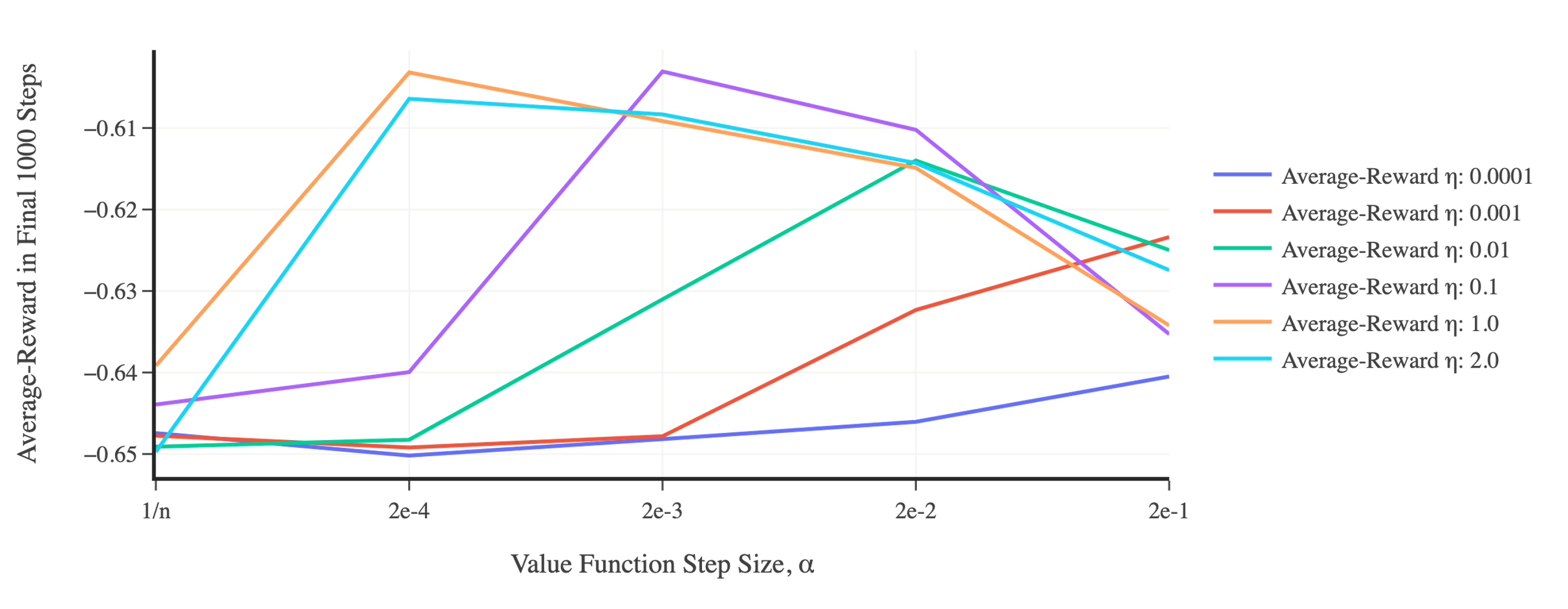
For the Differential Q-learning algorithm, we tested every combination of the value function step size, $\alpha\in\{\text{2e-1, 2e-2, 2e-3, 2e-4},1/n\}$ (where $1/n$ refers to a step size sequence that decreases the step size according to the time step, $n$), with the average-reward step size, $\eta\alpha$, where $\eta\in\{\text{1e-4, 1e-3, 1e-2, 1e-1, 1.0, 2.0}\}$, for a total of 30 unique combinations. Each combination was run 25 times using different random seeds, and the results were averaged across the runs. The resulting (averaged) average-reward over the last 1,000 time steps is displayed in Fig. C.1. As shown in the figure, a value function step size of 2e-4 and an average-reward $\eta$ of 1.0 resulted in the highest average-reward in the final 1,000 time steps in the red-pill blue-pill task. These are the parameters used to generate the results displayed in Fig. 4a). These parameters had a coefficient of variation with a magnitude of 2.33e-2 across the various random seed runs.

Refer to caption

Figure C.1: Step size tuning results for the red-pill blue-pill task when using the Differential Q-learning algorithm. The average-reward in the final 1,000 steps is displayed for various combinations of value function and average-reward step sizes.

For the RED CVaR Q-learning algorithm, we tested every combination of the value function step size, $\alpha\in\{\text{2e-1, 2e-2, 2e-3, 2e-4},1/n\}$, with the average-reward (in this case CVaR) $\eta\in\{\text{1e-4, 1e-3, 1e-2, 1e-1, 1.0, 2.0}\}$, and the VaR $\eta\in\{\text{1e-4, 1e-3, 1e-2, 1e-1, 1.0, 2.0}\}$, for a total of 180 unique combinations. Each combination was run 25 times using different random seeds, and the results were averaged across the runs. The resulting (averaged) reward CVaR over the last 1,000 time steps is displayed in Fig. C.2. As shown in the figure, combinations with larger step sizes converged to the optimal policy within the 100k time steps, and combinations with smaller step sizes did not (see Section C.4 for more discussion on this point). A value function step size of 2e-2, an average-reward (CVaR) $\eta$ of 1e-2, and a VaR $\eta$ of 1e-2 were used to generate the results displayed in Fig. 4a) and Fig. 5. These parameters had a coefficient of variation with a magnitude of 6.31e-3 across the various random seed runs.

Refer to caption

Figure C.2: Step size tuning results for the red-pill blue-pill task when using the RED CVaR Q-learning algorithm. Each plot represents a different $\eta_{{}_{\text{VaR}}}$ used: a) 2e-4; b) 2e-3; c) 2e-2; d) 2e-1; e) 1.0; f) 2.0. Within each plot, the reward CVaR in the final 1,000 steps is displayed for various combinations of value function and average-reward (in this case CVaR) step sizes.

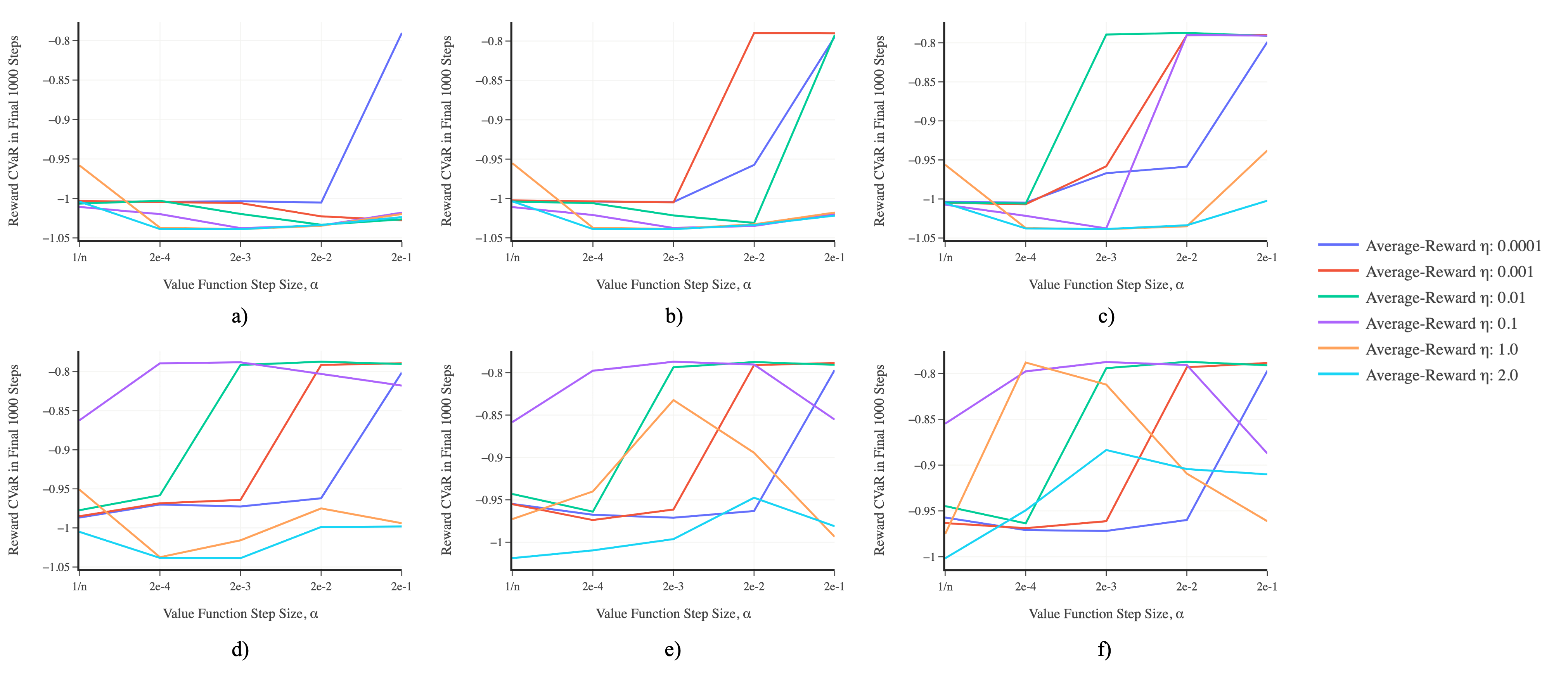
Fig. C.3a) shows the VaR and CVaR estimates as learning progresses when using the RED CVaR Q-learning algorithm with the same step sizes used in Figures 4a) and 5. We see that the resulting VaR and CVaR estimates generally track with what one would expect (similar values, with the VaR value being slightly larger than the CVaR value). We can see however that these estimates do not correspond to the actual VaR and CVaR values induced by the policy (as shown in Fig. 4a)). This is because, as previously mentioned, the solutions to the average-reward MDP Bellman equations (Equations (4), (5)), which in this case include the VaR and CVaR estimates, are only correct up to a constant. For comparison, we hard-coded the true VaR value and re-ran the same experiment, and found that the agent still converged to the correct policy, this time with a CVaR estimate that matched the actual CVaR value. Fig. C.3b) shows the results of this hard-coded VaR run.

Refer to caption


Figure C.3: The VaR and CVaR estimates as learning progresses when using the RED CVaR Q-learning algorithm: a) as per usual, and b) when hard-coding the VaR estimate to the true VaR.

C.3 Inverted pendulum experiment

In the second experiment, we consider the well-known inverted pendulum task, where an agent learns how to optimally balance an inverted pendulum. We chose this task because it provides us with opportunity to test our algorithm in an environment where: 1) we must use function approximation (given the large state and action spaces), and 2) where the policy for the optimal average-reward and the policy for the optimal reward CVaR is the same policy (i.e., the policy that best balances the pendulum will yield a stationary reward distribution with both the optimal average-reward and reward CVaR). This hence allows us to directly compare the performance of our RED algorithms to the regular Differential learning algorithms, as well as to gauge how function approximation affects the performance of our algorithms. For this task, we utilized a simple actor-critic architecture [2] as this allowed us to compare the performance of the (non-tabular) RED TD-learning algorithm with a (non-tabular) Differential TD-learning algorithm. This task is illustrated in Fig. 3b).

For this experiment, we ran both algorithms using various combinations of step sizes for each algorithm. We used a fixed CVaR parameter, $\tau$, of $0.1$. We set all initial guesses to zero. We ran the algorithms for 100k time steps. For simplicity, we used tile coding [2] for both the value function and policy parameterizations, where we parameterized a softmax policy. For each parameterization, we used 32 tilings, each with 8 X 8 tiles. By using a linear function approximator (i.e., tile coding), the gradients for the value function and policy parameterizations can be simplified as follows:

$$\nabla\hat{v}(s,\boldsymbol{w})=\boldsymbol{x}(s),$$ (C.7)
$$\nabla\text{ln}\pi(a\mid s,\boldsymbol{\theta})=\boldsymbol{x}_{h}(s,a)-\sum_{\xi\in\mathcal{A}}\pi(\xi\mid s,\boldsymbol{\theta})\boldsymbol{x}_{h}(s,\xi),$$ (C.8)

where $s\in\mathcal{S}$, $a\in\mathcal{A}$, $\boldsymbol{x}(s)$ is the state feature vector, and $\boldsymbol{x}_{h}(s,a)$ is the softmax preference vector.

For the RED CVaR Actor-Critic algorithm, we tested every combination of the value function step size, $\alpha\in\{\text{2e-2, 2e-3, 2e-4},1/n\}$ (where $1/n$ refers to a step size sequence that decreases the step size according to the time step, $n$), with $\eta$’s for the average-reward, VaR, and policy step sizes, $\eta\alpha$, where $\eta\in\{\text{1e-3, 1e-2, 1e-1, 1.0, 2.0}\}$, for a total of 500 unique combinations. Each combination was run 10 times using different random seeds, and the results were averaged across the runs. The resulting (averaged) reward CVaR over the last 1,000 time steps is displayed in Fig. C.4a) and the resulting (averaged) average-reward over the last 1,000 time steps is displayed in Fig. C.4b). As shown in the figure, most combinations allow the algorithm to converge to the optimal policy that balances the pendulum (as indicated by a reward CVaR and average-reward of zero). A value function step size of 2e-3, a policy $\eta$ of 1.0, an average-reward (CVaR) $\eta$ of 1e-2, and a VaR $\eta$ of 1e-2 were used to generate the results displayed in Fig. 4b). These parameters had a coefficient of variation with a magnitude of 2.85 across the various random seed runs.

For the Differential Actor-Critic algorithm, we tested every combination of the value function step size, $\alpha\in\{\text{2e-2, 2e-3, 2e-4},1/n\}$, with $\eta$’s for the average-reward and policy step sizes, $\eta\alpha$, where $\eta\in\{\text{1e-3, 1e-2, 1e-1, 1.0, 2.0}\}$, for a total of 100 unique combinations. Each combination was run 10 times using different random seeds, and the results were averaged across the runs. The resulting (averaged) reward CVaR over the last 1,000 time steps is displayed in Fig. C.4c) and the resulting (averaged) average-reward over the last 1,000 time steps is displayed in Fig. C.4d). As shown in the figure, most combinations allow the algorithm to converge to the optimal policy that balances the pendulum. A value function step size of 2e-3, a policy $\eta$ of 1.0, and an average-reward $\eta$ of 1e-3 were used to generate the results displayed in Fig. 4b). These parameters had a coefficient of variation with a magnitude of 2.16e-1 across the various random seed runs.

Refer to caption

Figure C.4: Step size tuning results for the inverted pendulum task when using the RED CVaR TD-learning and Differential TD-learning algorithms (through an actor-critic architecture). Each plot shows a histogram of either the reward CVaR or average-reward in the last 1,000 steps. More specifically, the histograms show: a) the reward CVaR when using the RED algorithm; b) the average-reward when using the RED algorithm; c) the reward CVaR when using the Differential algorithm; d) the average-reward when using the Differential algorithm.

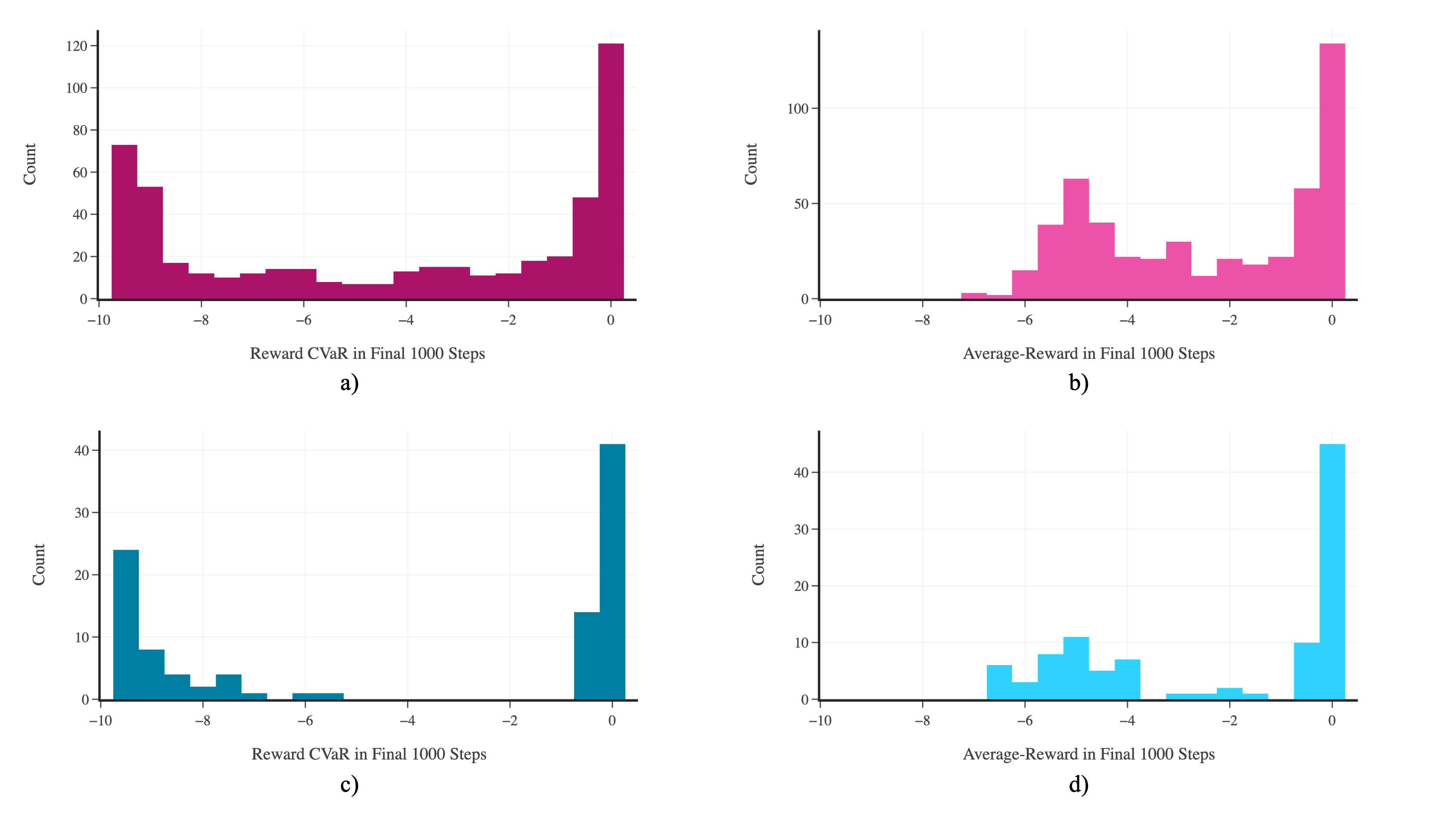
Fig. C.5a) shows the VaR and CVaR estimates as learning progresses when using the RED CVaR Actor-Critic algorithm with the same step sizes used in Fig. 4b). We see that the resulting VaR and CVaR estimates generally track with what one would expect (similar values, with the VaR value being slightly larger than the CVaR value). We can see however that these estimates do not correspond to the actual VaR and CVaR values induced by the policy (as shown in Fig. 4b)). This is because, as previously mentioned, the solutions to the average-reward MDP Bellman equations (Equations (4), (5)), which in this case include the VaR and CVaR estimates, are only correct up to a constant. For comparison, we hard-coded the true VaR value and re-ran the same experiment, and found that the agent still converged to the correct policy, this time with a CVaR estimate that more closely matched the actual CVaR value (note that in the inverted pendulum environment, rewards are capped at zero). Fig. C.5b) shows the results of this hard-coded VaR run.

Refer to caption

Figure C.5: The VaR and CVaR estimates as learning progresses when using the RED CVaR TD-learning algorithm (through an actor-critic architecture): a) as per usual, and b) when hard-coding the VaR estimate to the true VaR value. Note that in the inverted pendulum environment, rewards are capped at zero.

C.4 Commentary on experimental results

Red-Pill Blue-Pill: In the red-pill blue-pill task, we can see from Fig. C.1 that for combinations with large step sizes, the RED CVaR Q-learning algorithm was able to successfully learn a policy, within the 100k time steps, that prioritizes maximizing the reward CVaR over the average-reward, thereby achieving a sort of risk-awareness. However, for combinations with smaller step sizes, particularly for low VaR $\eta$’s, the algorithm did not converge in the allotted training period. We re-ran some of the combinations with constant step sizes for longer training periods, and found that the algorithm eventually converged to the risk-aware policy given enough training time. For combinations with the $1/n$ step size, we found that if the other step sizes in the combination were sufficiently small, the algorithm would not converge to the correct policy (even with more training time). This suggests that a more slowly-decreasing step size sequence should be used instead so that the algorithm has more time to find the correct policy before the step sizes in the sequence become too small.

Inverted Pendulum: In the inverted pendulum task, we can see from Fig. C.4 that both algorithms achieved similar performance, as shown by the similar histograms for both the reward CVaR and average-reward during the final 1,000 time steps. These results suggest that both algorithms converged to the same set of (sometimes sub-optimal) policies, as expected.

Overall: In both experiments, we can see that with proper hyperparameter tuning, the RED CVaR algorithms were able to consistently and reliably find the optimal CVaR policy. The VaR and CVaR estimates generally tracked with what one would expect (similar values, with the VaR value being slightly larger than the CVaR value). However, these estimates were not always the same as the actual VaR and CVaR values induced by the policy because the solutions to the average-reward MDP Bellman equations are only correct up to a constant. This is typically not a concern, given that the relative ordering of the policies is usually what is of interest.

C.5 Compute time and resources

For the red-pill blue-pill hyperparameter tuning, each case (which encompassed a specific combination of step sizes) took roughly 1 minute (total) to compute all 25 random seed runs for the case on a single CPU, for an approximate total of 4 CPU hours. For the inverted pendulum hyperparameter tuning, each case took roughly 5 minutes (total) to compute all 10 random seed runs for the case on a single CPU, for an approximate total of 50 CPU hours.

C.6 Algorithms

Below is the pseudocode for the algorithms used in the experiments discussed in this Appendix.

Algorithm 5 RED CVaR Q-Learning (Tabular)
  Input: the policy $\pi$ to be used (e.g., $\epsilon$-greedy)
  Algorithm parameters: step size parameters $\alpha$, $\eta_{{}_{\text{CVaR}}}$, $\eta_{{}_{\text{VaR}}}$, CVaR parameter $\tau$
  Initialize $Q(s,a)\>\forall s,a$ (e.g. to zero)
  Initialize CVaR arbitrarily (e.g. to zero)
  Initialize VaR arbitrarily (e.g. to zero)
  Obtain initial $S$
  while still time to train do
     $A\leftarrow$ action given by $\pi$ for $S$
     Take action $A$, observe $R,S^{\prime}$
     $\tilde{R}=\text{VaR}-\frac{1}{\tau}\max\{\text{VaR}-R,0\}-(\tau-\mathds{1}_{\{R<\text{VaR}\}})-(1-\tau)\left((1-\tau)-\mathds{1}_{\{R\geq\text{VaR}\}}\right)$
     $\delta=\tilde{R}-\text{CVaR}+\max_{a}Q(S^{\prime},a)-Q(S,A)$
     if $R\geq\text{VaR}$ then
        $\text{VaR}=\text{VaR}-\eta_{{}_{\text{VaR}}}\alpha\delta$
     else
        $\text{VaR}=\text{VaR}+\eta_{{}_{\text{VaR}}}\alpha(\frac{\tau}{1-\tau})\delta$
     end if
     $\text{CVaR}=\text{CVaR}+\eta_{{}_{\text{CVaR}}}\alpha\delta$
     $Q(S,A)=Q(S,A)+\alpha\delta$
     $S=S^{\prime}$
  end while
  return $Q$
Algorithm 6 Differential Q-Learning (Tabular)
  Input: the policy $\pi$ to be used (e.g., $\epsilon$-greedy)
  Algorithm parameters: step size parameters $\alpha$, $\eta$
  Initialize $Q(s,a)\>\forall s,a$ (e.g. to zero)
  Initialize $\bar{R}$ arbitrarily (e.g. to zero)
  Obtain initial $S$
  while still time to train do
     $A\leftarrow$ action given by $\pi$ for $S$
     Take action $A$, observe $R,S^{\prime}$
     $\delta=R-\bar{R}+\max_{a}Q(S^{\prime},a)-Q(S,A)$
     $\bar{R}=\bar{R}+\eta\alpha\delta$
     $Q(S,A)=Q(S,A)+\alpha\delta$
     $S=S^{\prime}$
  end while
  return $Q$
Algorithm 7 RED CVaR Actor-Critic
  Input: a differentiable state-value function parameterization $\hat{v}(s,\boldsymbol{w})$; a differentiable policy parameterization $\pi(a\mid s,\boldsymbol{\theta})$
  Algorithm parameters: step size parameters $\alpha$, $\eta_{\pi}$, $\eta_{{}_{\text{CVaR}}}$, $\eta_{{}_{\text{VaR}}}$, CVaR parameter $\tau$
  state-value weights $\boldsymbol{w}\in\mathbb{R}^{d}$ and policy weights $\boldsymbol{\theta}\in\mathbb{R}^{d^{\prime}}$ (e.g. to $\boldsymbol{0}$)
  Initialize CVaR arbitrarily (e.g. to zero)
  Initialize VaR arbitrarily (e.g. to zero)
  Obtain initial $S$
  while still time to train do
     $A\sim\pi(\cdot\mid S,\boldsymbol{\theta})$
     Take action $A$, observe $R,S^{\prime}$
     $\tilde{R}=\text{VaR}-\frac{1}{\tau}\max\{\text{VaR}-R,0\}-(\tau-\mathds{1}_{\{R<\text{VaR}\}})-(1-\tau)\left((1-\tau)-\mathds{1}_{\{R\geq\text{VaR}\}}\right)$
     $\delta=\tilde{R}-\text{CVaR}+\hat{v}(S^{\prime},\boldsymbol{w})-\hat{v}(S,\boldsymbol{w})$
     if $R\geq\text{VaR}$ then
        $\text{VaR}=\text{VaR}-\eta_{{}_{\text{VaR}}}\alpha\delta$
     else
        $\text{VaR}=\text{VaR}+\eta_{{}_{\text{VaR}}}\alpha(\frac{\tau}{1-\tau})\delta$
     end if
     $\text{CVaR}=\text{CVaR}+\eta_{{}_{\text{CVaR}}}\alpha\delta$
     $\boldsymbol{w}=\boldsymbol{w}+\alpha\delta\nabla\hat{v}(S,\boldsymbol{w})$
     $\boldsymbol{\theta}=\boldsymbol{\theta}+\eta_{\pi}\alpha\delta\nabla\text{ln}\pi(A\mid S,\boldsymbol{\theta})$
     $S=S^{\prime}$
  end while
  return $\boldsymbol{w}$, $\boldsymbol{\theta}$
Algorithm 8 Differential Actor-Critic
  Input: a differentiable state-value function parameterization $\hat{v}(s,\boldsymbol{w})$; a differentiable policy parameterization $\pi(a\mid s,\boldsymbol{\theta})$
  Algorithm parameters: step size parameters $\alpha$, $\eta_{\pi}$, $\eta_{{}_{\bar{R}}}$
  state-value weights $\boldsymbol{w}\in\mathbb{R}^{d}$ and policy weights $\boldsymbol{\theta}\in\mathbb{R}^{d^{\prime}}$ (e.g. to $\boldsymbol{0}$)
  Initialize $\bar{R}$ arbitrarily (e.g. to zero)
  Obtain initial $S$
  while still time to train do
     $A\sim\pi(\cdot\mid S,\boldsymbol{\theta})$
     Take action $A$, observe $R,S^{\prime}$
     $\delta=R-\bar{R}+\hat{v}(S^{\prime},\boldsymbol{w})-\hat{v}(S,\boldsymbol{w})$
     $\bar{R}=\bar{R}+\eta_{{}_{\bar{R}}}\alpha\delta$
     $\boldsymbol{w}=\boldsymbol{w}+\alpha\delta\nabla\hat{v}(S,\boldsymbol{w})$
     $\boldsymbol{\theta}=\boldsymbol{\theta}+\eta_{\pi}\alpha\delta\nabla\text{ln}\pi(A\mid S,\boldsymbol{\theta})$
     $S=S^{\prime}$
  end while
  return $\boldsymbol{w}$, $\boldsymbol{\theta}$

Appendix D Red-pill blue-pill environment

This Appendix contains the code for the red-pill blue-pill environment introduced in this work. The environment consists of a two-state MDP, where at every time step an agent can take either a red pill, which takes them to the ‘red world’ state, or a blue pill, which takes them to the ‘blue world’ state. Each state has its own characteristic reward distribution, and in this case, the red world state has a reward distribution with a lower (worse) mean but higher (better) CVaR compared to the blue world state. More specifically, the red world state reward distribution is characterized as a gaussian distribution with a mean of $-0.7$ and a standard deviation of $0.05$. The blue world state is characterized by a mixture of two gaussian distributions with means of $-1.0$ and $-0.2$, and standard deviations of $0.05$. We assume all rewards are non-positive.

The Python code for the environment is provided below:

import pandas as pd
import numpy as np
class EnvironmentRedPillBluePill:
def __init__(self, dist_2_mix_coefficient=0.5):
# set distribution parameters
self.dist_1 = {’mean’: -0.7, ’stdev’: 0.05}
self.dist_2a = {’mean’: -1.0, ’stdev’: 0.05}
self.dist_2b = {’mean’: -0.2, ’stdev’: 0.05}
self.dist_2_mix_coefficient = dist_2_mix_coefficient
# start state
self.start_state = np.random.choice(
[’redworld’,
’blueworld’]
)
def env_start(self, start_state=None):
# return initial state
if pd.isnull(start_state):
return self.start_state
else:
return start_state
def env_step(self, state, action, terminal=False):
if action == ’red_pill’:
next_state = ’redworld’
elif action == ’blue_pill’:
next_state = ’blueworld’
if state == ’redworld’:
reward = np.random.normal(loc=self.dist_1[’mean’],
scale=self.dist_1[’stdev’])
elif state == ’blueworld’:
dist = np.random.choice([’dist2a’, ’dist2b’],
p=[self.dist_2_mix_coefficient,
1 - self.dist_2_mix_coefficient])
if dist == ’dist2a’:
reward = np.random.normal(loc=self.dist_2a[’mean’],
scale=self.dist_2a[’stdev’])
elif dist == ’dist2b’:
reward = np.random.normal(loc=self.dist_2b[’mean’],
scale=self.dist_2b[’stdev’])
return min(0, reward), next_state, terminal