Regularized Robustly Reliable Learners and Instance Targeted Attacks

Regularized Robustly Reliable Learners and Instance Targeted Attacks

Abstract

Instance-targeted data poisoning attacks, where an adversary corrupts a training set to induce errors on specific test points, have raised significant concerns. Balcan et al. [2022] proposed an approach to addressing this challenge by defining a notion of robustly-reliable learners that provide per-instance guarantees of correctness under well-defined assumptions, even in the presence of data poisoning attacks. They then give a generic optimal (but computationally inefficient) robustly-reliable learner as well as a computationally efficient algorithm for the case of linear separators over log-concave distributions.

In this work, we address two challenges left open by Balcan et al. [2022]. The first is that the definition of robustly-reliable learners in Balcan et al. [2022] becomes vacuous for highly-flexible hypothesis classes: if there are two classifiers $h_{0},h_{1}\in\mathcal{H}$ both with zero error on the training set such that $h_{0}(x)\neq h_{1}(x)$, then a robustly-reliable learner must abstain on $x$. We address this problem by defining a modified notion of regularized robustly-reliable learners that allows for nontrivial statements in this case. The second is that the generic algorithm of Balcan et al. [2022] requires re-running an ERM oracle (essentially, retraining the classifier) on each test point $x$, which is generally impractical even if ERM can be implemented efficiently. To tackle this problem, we show that at least in certain interesting cases we can design algorithms that can produce their outputs in time sublinear in training time, by using techniques from dynamic algorithm design.

1 Introduction

As Machine Learning and AI are increasingly used for critical decision-making throughout society, it is becoming more important than ever that these systems be trustworthy and reliable. This means they should know (and say) when they are unsure, they should be able to provide real explanations for their answers and why those answers should be trusted (not just how the prediction was made), and they should be robust to malicious or unusual training data and to adversarial or unusual examples at test time.

Balcan et al. [2022] proposed an approach to addressing this problem by defining a notion of robustly-reliable learners that provide per-instance guarantees of correctness under well-defined assumptions, even in the presence of data poisoning attacks. This notion builds on the definition of reliable learners by Rivest and Sloan [1988]. In brief, a robustly-reliable learner $\mathcal{L}$ for some hypothesis class $\mathcal{H}$, when given a (possibly corrupted) training set $S^{\prime}$, produces a classifier $\mathcal{L}_{S^{\prime}}$ that on any example $x$ outputs both a prediction $y$ and a confidence level $k$. The interpretation of the pair $(y,k)$ is that $y$ is guaranteed to equal the correct label $f^{*}(x)$ if (a) the target function $f^{*}$ indeed belongs to $\mathcal{H}$ and (b) the set $S^{\prime}$ contains at most $k$ corrupted points; here, $k<0$ corresponds to abstaining. Balcan et al. [2022] then provide a generic pointwise-optimal algorithm for this problem: one that for each $x$ outputs the largest possible confidence level of any robustly-reliable learner. They also give efficient algorithms for the important case of homogeneous linear separators over uniform and log-concave distributions, as well as analysis of the probability mass of points for which it outputs large values of $k$.

In this work, we address two challenges left open by Balcan et al. [2022]. The first is that the definition of robustly-reliable learners in Balcan et al. [2022] becomes vacuous for highly-flexible hypothesis classes: if there are two classifiers $h_{0},h_{1}\in\mathcal{H}$ both with zero error on the training set such that $h_{0}(x)\neq h_{1}(x)$, then a robustly-reliable learner must abstain on $x$. We address this problem by defining a modified notion of regularized robustly-reliable learners that allows for nontrivial statements in this case. The second is that the generic algorithm of Balcan et al. [2022] requires re-running an ERM oracle (essentially, retraining the classifier) on each test point $x$, which is generally impractical even if ERM can be implemented efficiently. To tackle this problem, we show that at least in certain interesting cases we can design algorithms that can make predictions in time sublinear in training time, by using techniques from dynamic algorithm design, such as Bosek et al. [2014].

1.1 Main contibutions

Our main contributions are three-fold.

1. The first is a definition of a regularized robustly-reliable learner, and of the region of points it can certify, that is appropriate for highly-flexible hypothesis classes. We then analyze the largest possible set of points that any regularized robustly-reliable learner could possibly certify, and provide a generic pointwise-optimal algorithm whose regularized robustly-reliable region ($\rm R^{4}$) matches this optimal set (${\rm OPTR^{4}}$).

2. The second is an analysis of the probability mass of this ${\rm OPTR^{4}}$ set in some intersting special cases, proving sample complexity bounds on the number of training examples needed (relative to the data poisoning budget of the adversary and the complexity of the target function) in order for ${\rm OPTR^{4}}$ to w.h.p. have a large probability mass.

3. Finally, the third is analysis of efficient regularized robustly-reliable learning algorithms for interesting cases, with a special focus on algorithms that are able to output their reliability guarantees more efficiently than re-training the entire classifier. In one case we do this through a bi-directional dynamic programming algorithm, and in another case by utilizing algorithms for maximum matching that are able to quickly re-establish the maximum matching when a few nodes are added to or deleted from the graph.

In a bit more detail, for a given complexity measure $\mathcal{C}$, a regularized robustly-reliable learner $\mathcal{L}$ is given as input a (possibly corrupted) training set $S^{\prime}$ and outputs a function (an “extended classifier”) $\mathcal{L}_{S^{\prime}}$. The extended classifier $\mathcal{L}_{S^{\prime}}$ takes in two inputs: a test example $x$ and a poisoning budget $b$, and outputs a prediction $y$ along with two complexity levels $c_{\text{low}}$ and $c_{\text{high}}$. The meaning of the triple $(y,c_{\text{low}},c_{\text{high}})$ is that $y$ is guaranteed to be the correct label $f^{*}(x)$ if the training set $S^{\prime}$ contains at most $b$ poisoned points and the complexity of the target function $f^{*}$ is less than $c_{\text{high}}$. Moreover, there should exist a classifier $f$ of complexity at most $c_{low}$ that makes at most $b$ mistakes on $S^{\prime}$ and has $f(x)=y$. Thus, if we, as a user, believe that a complexity at or above $c_{high}$ is “unnatural” and that the training set should contain at most $b$ corrupted points, then we can be confident in the predicted label $y$. We then analyze the set of points for which $c_{low}\leq c<c_{high}$ for a given complexity level $c$, and show there exists an algorithm that is simultaneously optimal in terms of the size of this set for all values of $c$.

Note that the above description has been treating the complexity function $\mathcal{C}$ as a data-independent notion; we also consider data-dependent notions of complexity, including notions that involve the test point itself.

1.2 Context and Related Work

Learning from malicious noise. The malicious noise model was introduced and analyzed in in Valiant [1985] Kearns and Li [1993], Bshouty et al. [2002], Klivans et al. [2009], Awasthi et al. [2018]. However, the focus of this work was on the overall error rate of the learned classifier, rather than on instance-wise guarantees that could be provided on individual predictions.

Instance targeted poisoning attacks. Instance-targeted poisoning attacks were first introduced by Barreno et al. [2006]. Subsequent work by Suciu et al. [2018] and Shafahi et al. [2018] demonstrated empirically that such attacks can be highly effective, even when the adversary only adds correctly-labeled data to the training set (known as “clean-label attacks”). These targeted poisoning attacks have attracted considerable attention in recent years due to their potential to compromise the trustworthiness of learning systems Geiping et al. [2021], Mozaffari-Kermani et al. [2015],Chen et al. [2017]. Theoretical research on defenses against instance-targeted poisoning attacks has largely focused on developing stability certificates, which indicate when an adversary with a limited budget cannot alter the resulting prediction. For instance, Levine and Feizi [2021] suggest partitioning the training data into $k$ segments, training distinct classifiers on each segment, and using the strength of the majority vote from these classifiers as a stability certificate, as any single poisoned point can affect only one segment. Additionally, Gao et al. [2021] formalize various types of adversarial poisoning attacks and explore the problem of providing stability certificates for them in both distribution-independent and distribution-specific scenarios. Moreover, Balcan et al. [2022] further studied such attacks and in contrast to the previous results that certify when a budget-limited adversary could not change the learner’s prediction, their work focuses on certifying the prediction made is correct. The model of Balcan et al. [2022] can be seen as a generalization of the reliable-useful learning framework presented by Rivest and Sloan [1988] and the perfect selective classification model proposed by El-Yaniv and Wiener [2010], which focuses on the simpler scenario of learning from noiseless data, extending it to the more complex context of noisy data and adversarial poisoning attacks.

2 Formal Setup

We consider a learner aiming to learn an unknown target function $f^{*}:\mathcal{X}\rightarrow\mathcal{Y}$, where $\mathcal{X}$ denotes the instance space and $\mathcal{Y}$ the label space. The learner is given a training set $S^{\prime}=\{\{(x_{i},y_{i})\}_{i=1}^{n}|x\in\mathcal{X},y\in\mathcal{Y}\}$, which might have been poisoned by a malicious adversary. Specifically, we assume $S^{\prime}$ consists of an original dataset $S$ labeled according to $f^{*}$, with possibly additional examples, whose labels need not match $f^{*}$, added by an adversary. For original dataset $S$ and non-negative integer $b$, let $\mathcal{A}_{b}(S)$ denote the possible training sets that could be produced by an attacker with corruption budget $b$. That is, $\mathcal{A}_{b}(S)$ consists of all $S^{\prime}$ that could be produced by adding $b$ points to $S$. Given the training set $S^{\prime}$ and test point $x$, the learner’s goal will be to output a label $y$ along with a guarantee that $y=f^{*}(x)$ so long as $f^{*}$ is sufficiently “simple” and the adversary’s corruption budget was sufficiently small. Conceptually, we will imagine that the adversary might have been using its entire corruption budget specifically to cause us to make an error on $x$. Our basic definitions will not require that the original set $S$ be drawn iid (or that the test point $x$ be drawn from the same distribution) but our guarantees on the probability mass of points for which a given strength of guarantee can be given will require such assumptions.

Complexity measures

To establish a framework where certain classifiers or classifications are considered more natural than others, we assume access to a complexity measure $\mathcal{C}$ that formalizes this degree of un-naturalness. We consider several distinct types of complexity measures.

1. Data independent: Each classifier $h$ has a well-defined real-valued complexity $\mathcal{C}(h)$. For example, in $\mathbb{R}^{1}$, a natural measure of complexity of a Boolean function is the number of alternations between positive and negative regions (See Definition 8).

2. Test data dependent: Such complexity is a function of the classifier $h$, and the test point $x_{test}$. For example, let $r$ denote the distance of $x_{test}$ to $h$’s decision boundary; we then might define complexity $\mathcal{C}(h,x_{test})=\frac{1}{r}$ (See Definition 9).

3. Training data dependent: This complexity is a function of the classifier $h$, the training set $S^{\prime}$ and the corruption budget $b$. An example of this measure is the Interval Probability Mass complexity, detailed in the Appendix (See Definition 12).

4. Training and test data dependent: Here, complexity is a function of the classifier $h$, the training set $S^{\prime}$, the corruption budget $b$, and the test point $x_{test}$. For instance, we might be interested in the margin $r$ of a classifier with respect to both the training set and the test point, and define complexity to be $\frac{1}{r}$

   (See Definition 10).

In section 4, and Appendix 8.1, we introduce several complexity measures across all four types, for assessing the structure and behavior of classifiers. Next, we define a learning rule, Empirical Complexity Minimization, analogous to ERM, that leverages these measures. This rule selects a hypothesis of minimum complexity subject to the constraint of making no more than $b$ mistakes on the training set.

Definition 1 (Empirical Complexity Minimization).

Given a complexity measure $\mathcal{C}$, a hypothesis class $\mathcal{H}$, a training set $S^{\prime}=\{(x_{1},y_{1}),(x_{2},y_{2}),...,(x_{n},y_{n})\}$, and a mistake budget $b$, let $\mathcal{H}_{b,S^{\prime}}$ be the set of hypotheses that make at most $b$ mistakes on $S^{\prime}$:

$$\mathcal{H}_{b,S^{\prime}}=\{h\mid\sum_{i=1}^{n}\mathbf{1}[h(x_{i})\neq y_{i}]\leq b\}.$$

For a data-independent complexity measure, we define the ECM learning rule to choose

$$h_{\text{ECM}}=\arg\min_{h\in\mathcal{H}_{b,S^{\prime}}}\mathcal{C}(h)$$

For training-data-dependent complexity measures, we replace $\mathcal{C}(h)$ with $\mathcal{C}(h,S^{\prime},b)$. When the complexity measure is test-data-dependent (or training-and-test dependent), we define the ECM learning rule to output just the complexity value, rather than a hypothesis.

$$\underset{h\in\mathcal{H}_{b,S^{\prime}}:h(x_{\text{test}})=y_{\text{test}}}{\min}\mathcal{C}(h,x_{\text{test}})\qquad\mbox{or}\qquad\underset{h\in\mathcal{H}_{b,S^{\prime}}:h(x_{\text{test}})=y_{\text{test}}}{\min}\mathcal{C}(h,S^{\prime},b,x_{\text{test}}).$$

We now define the notion of a regularized-robustly-reliable learner in the face of instance-targeted attacks. This learner, for any given test example $x_{\text{test}}$, outputs both a prediction $y$ and values $c_{\text{low}}$ and $c_{\text{high}}$, such that $y$ is guaranteed to be correct so long as the target function $f^{*}$ has complexity less than $c_{\text{high}}$ and the adversary has at most corrupted $b$ points. Moreover, there should exist a candidate classifier of complexity at most $c_{\text{low}}$.

Definition 2 (Regularized Robustly Reliable Learner).

The learner $\mathcal{L}$ has access to a corruption $S^{\prime}$ of some true sample set $S\subset(\mathcal{X},\mathcal{Y})$. The learner $\mathcal{L}$ is regularized-robustly-reliable w.r.t. a complexity measure $\mathcal{C}$ if, given $S^{\prime}$, the learner outputs a function $\mathcal{L}_{S^{\prime}}$ with the following properties: Given a test point $x_{\text{test}}$ and mistake budget $b$, $\mathcal{L}_{S^{\prime}}$ outputs a label $y$ along with complexity levels $c_{\text{low}},c_{\text{high}}$ such that

1. There exists a classifier $h$ of complexity $c_{low}$ with at most $b$ mistakes on $S^{\prime}$ such that $h(x_{test})=y$, and

2. There is no classifier $h^{\prime}$ of complexity less than $c_{high}$ with at most $b$ mistakes on $S^{\prime}$ such that $h^{\prime}(x_{test})\neq y$.

So, if $\mathcal{L}_{S^{\prime}}(x_{\text{test}},b)=(y,c_{\text{low}},c_{\text{high}})$, then we are guaranteed that $y=f^{*}(x_{test})$ if $f^{*}$ has complexity less than $c_{\text{high}}$ and $S^{\prime}\in\mathcal{A}_{b}(S)$. Moreover, there should exist a classifier $h$ of complexity $c_{low}$ with at most $b$ mistakes on $S^{\prime}$ such that $h(x_{test})=y$.

Remark 1.

In Definition 2, when the learner outputs a value $c_{\text{high}}$ that is less than or equal to $c_{\text{low}}$, we interpret it as “abstaining.”

Definition 3 (Exact Regularized Robustly Reliable Learner).

We say the learner $\mathcal{L}$ is Exact Regularized Robustly Reliable if $c_{\text{high}}$ is the smallest value for which there exist functions $f,f^{\prime}$ of complexity $c_{\text{high}}$ that each make at most $b$ mistakes on $S^{\prime}$ and $f(x_{test})\neq f^{\prime}(x_{test})$. And, $c_{\text{low}}$ is the complexity of the minimum-complexity function possible that makes at most $b$ mistakes on $S^{\prime}$.

We now define the regularized robustly reliable region for a learner satisfying Definition 2.

Definition 4 (Empirical Regularized Robustly Reliable Region).

For learner $\mathcal{L}$, given a (possibly corrupted) dataset $S^{\prime}$, a poisoning budget $b$, and a complexity bound $c$ with respect to a complexity measure $\mathcal{C}$, the empirical regularized robustly reliable region ${\rm\widehat{R^{4}}}_{\mathcal{L}}(S^{\prime},b,c)$ is the set of points $x$ for which $\mathcal{L}_{S^{\prime}}(x,b)$ outputs $c_{low},c_{high}$ such that $c_{low}\leq c<c_{high}$.

Remark 2.

If the target function $f^{*}$ has complexity $c$, we will say the learner $\mathcal{L}$’s prediction is “vacuous” on a point $x$ if $x\notin{\rm\widehat{R^{4}}}_{\mathcal{L}}(S^{\prime},b,c)$.

It turns out that similarly to Balcan et al. [2022], one can characterize the largest possible set ${\rm\widehat{R^{4}}}_{\mathcal{L}}(S^{\prime},b,c)$ in terms of agreement regions. We describe the characterization below, and prove its optimality in Section 3.

Definition 5 (Optimal Empirical Regularized Robustly Reliable Region).

Given dataset $S^{\prime}$, poisoning budget $b$, and complexity bound $c$, the optimal empirical regularized robustly reliable region ${\rm\widehat{OPTR^{4}}}(S^{\prime},b,c)$ is the agreement region of the set of functions of complexity at most $c$ that make at most $b$ mistakes on $S^{\prime}$. If there are no such functions, then ${\rm\widehat{OPTR^{4}}}(S^{\prime},b,c)$ is undefined.

In the next section we give a regularized robustly reliable learner $\mathcal{L}$ satisfying ${\rm\widehat{R^{4}}}_{\mathcal{L}}(S^{\prime},b,c)={\rm\widehat{OPTR^{4}}}$, and show how it can be implemented efficiently given access to an ECM oracle for a given complexity measure $\mathcal{C}$. We then prove that any other regularized robustly reliable learner $\mathcal{L}^{\prime}$ must have ${\rm\widehat{R^{4}}}_{\mathcal{L}^{\prime}}(S^{\prime},b,c)\subseteq{\rm\widehat{OPTR^{4}}}$. This justifies the use of the term optimal in definition 5.

3 Regularized Robustly Reliable Learners for Instance-Targeted Adversaries

Recall that a regularized robustly reliable (RRR) learner $\mathcal{L}$ is given a sample $S^{\prime}$ and outputs a function $\mathcal{L}_{S^{\prime}}(x)=(y,c_{\text{low}},c_{\text{high}})$ such that if $S^{\prime}=\mathcal{A}_{b}(S)$ for some (unknown) uncorrupted sample $S$ labeled by some (unknown) target concept, $f^{*}$, and $\mathcal{C}(f^{*})\in[c_{\text{low}},c_{\text{high}})$, then $y=f^{*}(x)$.

Theorem 1.

For any RRR learner $\mathcal{L}^{\prime}$ we have ${\rm\widehat{R^{4}}}_{\mathcal{L}^{\prime}}(S^{\prime},b,c)\subseteq{\rm\widehat{OPTR^{4}}}(S^{\prime},b,c)$. Moreover, there exists an RRR learner $\mathcal{L}$ such that ${\rm\widehat{R^{4}}}_{\mathcal{L}}(S^{\prime},b,c)={\rm\widehat{OPTR^{4}}}(S^{\prime},b,c)$.

Proof.

First, consider any $x\not\in{\rm\widehat{OPTR^{4}}}(S^{\prime},b,c)$. This means there exist $h_{0}$ and $h_{1}$ of complexity at most $c$, each making at most $b$ mistakes on $S^{\prime}$, such that $h_{0}(x)\neq h_{1}(x)$. In particular, this implies that for any label $y$, there exists a classifier $h^{\prime}$ of complexity at most $c$ with at most $b$ mistakes on $S^{\prime}$ such that $h^{\prime}(x)\neq y$. So, for any RRR learner $\mathcal{L}^{\prime}$, by part (b) of Definition 2, $\mathcal{L}^{\prime}$ cannot output $c_{high}>c$, and therefore $x\not\in{\rm\widehat{R^{4}}}_{\mathcal{L}^{\prime}}(S^{\prime},b,c)$. This establishes that ${\rm\widehat{R^{4}}}_{\mathcal{L}^{\prime}}(S^{\prime},b,c)\subseteq{\rm\widehat{OPTR^{4}}}(S^{\prime},b,c)$.

For the second part of the theorem, let us first consider complexity measures that are not test-data dependent. In that case, consider a learner $\mathcal{L}$ that given $S^{\prime}$ finds the classifier $h_{S^{\prime}}$ of minimum complexity that makes at most $b$ mistakes on $S^{\prime}$ and then uses it on test point $x$. Specifically, it outputs $(y,c_{low},c_{high})$ where $y=h_{S^{\prime}}(x)$, $c_{low}=\mathcal{C}(h_{S^{\prime}})$, and

$$c_{high}=\min\{\mathcal{C}(h):h\mbox{ makes at most }b\mbox{ mistakes on }S^{\prime}\mbox{ and }h(x)\neq h_{S^{\prime}}(x)\}.$$

By construction, $\mathcal{L}$ is a RRR learner. Now, if $x\in{\rm\widehat{OPTR^{4}}}(S^{\prime},b,c)$ then this learner $\mathcal{L}$ will output $(y,c_{low},c_{high})$ such that $c_{low}\leq c$ and $c_{high}>c$. That is because $x$ is in the agreement region of classifiers of complexity at most $c$ that make at most $b$ mistakes on $S^{\prime}$, which means that any classifier making at most $b$ mistakes on $S^{\prime}$ that outputs a label different than $y$ on $x$ must have complexity strictly larger than $c$. So, $x\in{\rm\widehat{R^{4}}}_{\mathcal{L}}(S^{\prime},b,c)$. This establishes that ${\rm\widehat{R^{4}}}_{\mathcal{L}}(S^{\prime},b,c)\supseteq{\rm\widehat{OPTR^{4}}}(S^{\prime},b,c)$, which together with the first part implies that ${\rm\widehat{R^{4}}}_{\mathcal{L}}(S^{\prime},b,c)={\rm\widehat{OPTR^{4}}}(S^{\prime},b,c)$

If the complexity measure is test data dependent, the learner $\mathcal{L}$ instead works as follows. First, augment $S^{\prime}$ by adding $b+1$ copies of $x_{\text{test}}$ each labeled as $y_{\text{test}}=y_{1}$. This ensures that the mistake budget of the ECM algorithm is not depleted by the test point $x_{\text{test}}$, as the additional copies force the algorithm to allocate its mistake budget elsewhere. We then run the ECM algorithm on this modified dataset, and denote the complexity measure returned by the oracle as $c_{y_{1}}$. Next, we repeat this procedure for the remaining possible labels $y_{2},\dots,y_{m}$, each time augmenting the dataset with $b+1$ copies of $x_{\text{test}}$ labeled according to $y_{i}$. Let the corresponding complexity measures returned by the ECM oracle be denoted as $c_{y_{2}},\dots,c_{y_{m}}$. Without loss of generality, assume $c_{y_{1}}\leq c_{y_{2}}\leq\dots\leq c_{y_{m}}$. We define:

$$c_{\text{low}}=c_{y_{1}},\quad c_{\text{high}}=c_{y_{2}}$$

where $c_{\text{low}}$ represents the minimum complexity value among the different labelings of $x_{\text{test}}$, and $c_{\text{high}}$ represents the second-lowest complexity value. ∎

Remark 3.

Note that the optimal RRR learner $\mathcal{L}$ in Theorem 1 in principle may need to re-train on each test point $x$ in order to compute $c_{high}$ (and if the complexity measure is test-point-dependent, $c_{low}$ as well). In particular, it needs to identify (the complexity of) the minimum-complexity function making at most $b$ mistakes on $S^{\prime}$ that would label $x$ differently from $h_{S^{\prime}}$. In Sections 4 we will see efficient algorithms for certain natural complexity measures where this can be done efficiently.

Definition 5 and Theorem 1 gave guarantees in terms of the observed sample $S^{\prime}$. We now consider guarantees in terms of the original clean dataset $S$, defining the set of points that the learner will be able to correctly classify and provide meaningful confidence values no matter how an adversary corrupts $S$ with up to $b$ poisoned points. For simplicity and to keep the definitions clean, we assume for the remaining portion of this section that $\mathcal{C}$ is non-data-dependent.

Definition 6 (Regularized Robustly Reliable Region).

Given a complexity measure $\mathcal{C}$, a sample $S$ labeled by some target function $f^{*}$ with $\mathcal{C}(f^{*})=c$, and a poisoning budget $b$, the regularized robustly reliable region $R^{4}_{\mathcal{L}}(S,b,c)$ for learner $\mathcal{L}$ is the set of points $x\in\mathcal{X}$ such that for all $S^{\prime}\in\mathcal{A}_{b}(S)$ we have $\mathcal{L}_{S^{\prime}}(x,b)=(y,c_{\text{low}},c_{\text{high}})$ with $c_{\text{low}}\leq c<c_{\text{high}}$.

Remark 4.

$R^{4}_{\mathcal{L}}(S,b,c)=\bigcap_{S^{\prime}\in\mathcal{A}_{b}(S)}{\rm\widehat{R^{4}}}_{\mathcal{L}}(S^{\prime},b,c)$.

Definition 7 (Optimal Regularized Robustly Reliable Region).

Given a complexity measure $\mathcal{C}$, a dataset $S$ labeled by some target function $f^{*}$, with $\mathcal{C}(f^{*})=c$, and a poisoning budget $b$, the optimal regularized robustly reliable region ${\rm OPTR^{4}}(S,b,c)$ is the agreement region of the set of functions of complexity at most $c$ that make at most $b$ mistakes on $S$. If there are no such functions, then ${\rm OPTR^{4}}(S^{\prime},b,c)$ is undefined.

Theorem 2.

For any RRR learner $\mathcal{L}^{\prime}$, we have $R^{4}_{\mathcal{L}^{\prime}}(S,b,\mathcal{C}(f^{*}))\subseteq\text{OPTR}^{4}(S,b,\mathcal{C}(f^{*}))$. Moreover, there exists an RRR learner $\mathcal{L}$ such that for any dataset $S$ labeled by (unknown) target function $f^{*}$, we have $R^{4}_{\mathcal{L}}(S,b,\mathcal{C}(f^{*}))={\rm OPTR^{4}}(S,b,\mathcal{C}(f^{*}))$.

Proof.

For the first direction, consider $x\notin\text{OPTR}^{4}(S,b,\mathcal{C}(f^{*}))$. By definition, there is some $h$ with $\mathcal{C}(h)\leq\mathcal{C}(f^{*})$ that makes at most $b$ mistakes on $S$ and has $h(x)\neq f^{*}(x)$. Now, consider an adversary that adds no poisoned points, so that $S^{\prime}=S$. In this case, such $h$ makes at most $b$ mistakes on $S^{\prime}$, as well. Hence, by definition, $c_{\text{high}}\leq\mathcal{C}(f^{*})$ and so $x\notin R^{4}_{\mathcal{L}}(S,b,c)$. Hence, $R^{4}_{\mathcal{L}}(S,b,c)\subseteq\text{OPTR}^{4}(S,\mathcal{C}(f^{*}),b)$.

For the second direction, consider a learner $\mathcal{L}$ training set $S^{\prime}$, finds the classifier $h_{S^{\prime}}$ of minimum complexity that makes at most $b$ mistakes on $S^{\prime}$ and then uses it on test point $x$. Specifically, it outputs $(y,c_{\text{low}},c_{\text{high}})$ where $y=h_{S^{\prime}}(x)$,

$$c_{\text{low}}=\mathcal{C}(h_{S^{\prime}})$$

and

$$c_{\text{high}}=\min\{\mathcal{C}(h):h\text{ makes at most }b\text{ mistakes on }S^{\prime}\text{ and }h(x)\neq h_{S^{\prime}}(x)\}.$$

By construction, $\mathcal{L}$ satisfies Definition 2 and so is a RRR learner. Now, suppose indeed $S^{\prime}\in\mathcal{A}_{b}(S)$ for a true set $S$ labeled by target function $f^{*}$. Then $f^{*}$ makes at most $b$ mistakes on $S^{\prime}$, so $\mathcal{L}$ will output $c_{\text{low}}\leq\mathcal{C}(f^{*})$. Moreover, if $x\in\text{OPTR}^{4}(S,f^{*},b)$, then any classifier $h$ with $h(x)\neq f^{*}(x)$ either has complexity strictly greater than $f^{*}$ or makes more than $b$ mistakes on $S$ (and therefore more than $b$ mistakes on $S^{\prime}$). Therefore, $\mathcal{L}$ will output $c_{\text{high}}>\mathcal{C}(f^{*})$ and have $y=f^{*}(x)$. So, $x\in R^{4}_{\mathcal{L}}(S,b,\mathcal{C}(f^{*}))$. Therefore, ${\rm OPTR^{4}}(S,b,\mathcal{C}(f^{*}))\subseteq R^{4}_{\mathcal{L}}(S,b,\mathcal{C}(f^{*}))$. ∎

Remark 5.

Notice that the adversary’s optimal strategy with respect to $R^{4}$ is to add no points. That is because the learner needs to consider all classifiers of a given complexity that make at most $b$ mistakes on its training set, and adding new points can only make this set of classifiers smaller.

4 Regularized Robustly Reliable Learners with Efficient Algorithms

In this section, we present efficient algorithms for implementing exact regularized robustly reliable learners (Definition 3) for a variety of complexity measures.

We provide more examples in the Appendix. Our algorithms do not require retraining for a new test point unless the measure is test data dependent.

4.1 Number of Alternations

We first consider the Number of Alternations complexity measure, giving an efficient algorithm as well as analyzing the sample-complexity for having a large regularized robustly reliable region.

Definition 8 (Number of Alterations).

The number of alterations of a function $f:\mathbb{R}\to\{-1,+1\}$ is the number of times the function’s output changes between +1 and -1 as the input variable increases from negative to positive infinity.

Number of Alterations is a data-independent measure. A higher number of alterations implies a more intricate decision boundary, as the classifier switches between classes more frequently. For instance, if $f$ is the sign of a degree $d$ polynomial, then it can have at most $d$ alternations.

Example 1 (Number of Alterations).

Consider the dataset in Figure 1, assuming there is no adversary, it is impossible to classify these points with any function that has less than 7 alterations.

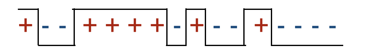
Figure 1: Number of Alterations with $\mathbb{R}\to\{+,-\}$ Data

We are interested in generating a guarantee for the test point in Figure 2.

Figure 2: Test point arrives

Our guarantee is as follows: The learner outputs a label alongside a complexity interval. So long as the complexity of the target function belongs to the given interval and the adversary has corrupted at most $b$ of the training data points, our prediction is correct (see Table 5).

Mistake Budget	Label	$(c_{\text{low}},c_{\text{high}})$
$b=0$	$+$	$[7,9)$
$b=1$	$+$	$[5,7)$
$b=2$	$+$	$[3,5)$
$b=3$	$+$	$[2,4)$
$b=4$	$+$	$[1,3)$
$b=5$	$+$	$[1,2)$
$b=6$	None	$\{1\}$
$b=7,8$	$-$	$[0,1)$
$b=9,10,11,12,13,14,15,16$	None	$\{1\}$

Table 1: Guarantee for the test point in Figure 2 and the complexity measure Number of Alterations.

Theorem 3.

For binary classification, an exact regularized-robustly-reliable learner (Definition 3) can be implemented efficiently for complexity measure Number of Alterations (Definition 8).

Proof sketch.  The high-level idea is to perform bi-directional Dynamic Programming on the training data. A left-to-right DP computes, for each point $i$ and each $j\leq b$, the minimum-complexity solution that makes $j$ mistakes up to that point (that is, on points $0,1,...,i$) and labels $i$ as positive, as well as the minimum-complexity solution that makes $j$ mistakes so far and labels $i$ as negative. A right-to-left DP does the same but in right-to-left order. Then, when a test point $x$ arrives, we can use the DP tables to compute the values $y,c_{low},c_{high}$ in time $O(b)$, without needing to re-train on the training data. In particular, we just need to consider all ways of partitioning the mistake-budget $b$ into $j$ mistakes on the left and $b-j$ mistakes on the right, and then using the DP tables to select the best choice. The full proof is given in Appendix 8.2.1. We now analyze the sample complexity for having a large ${\rm OPTR^{4}}$ when data is iid.

Theorem 4.

Suppose the Number of Alterations (Definition 8) of the target function is $c$. For any $\epsilon,\delta\in(0,1)$, and any mistake budget $b$, if the size of the (clean) sample $S\sim\mathcal{D}^{m}$ is at least $\tilde{O}\left(\frac{(b+1)c}{\epsilon}\right)$, then

with probability at least $1-\delta$, the optimal regularized robustly reliable region, ${\rm OPTR^{4}}(S,c,b)$, contains at least a $1-\epsilon$ probability mass of the distribution.

The proof is given in Appendix 8.2.2.

Remark 6.

The theorem above shows if $m=\tilde{O}\left(\frac{(b+1)c}{\epsilon}\right)$, then there exists a regularized robustly reliable (RRR) learner $\mathcal{L}$ such that given any $S^{\prime}\in\mathcal{A}_{b}(S)$ for a clean dataset $S$ labeled by a target function of complexity $c$, with probability at least $1-\delta$ its regularized robustly reliable region, $R^{4}_{\mathcal{L}}(S,b,c)$, contains at least $1-\epsilon$ of probability mass. Hence, with probability at least $1-\delta$ such learner generates non-vacuous guarantees a $1-\epsilon$ fraction of the time.

4.2 Local Margin

We now study a test-data-dependent measure.

Definition 9 (Local Margin).

Given a metric space $(\mathcal{M},d_{\mathcal{M}})$, for a classifier with a decision function $f:\mathcal{X}\to\mathcal{Y}$, where $\mathcal{X}$ is the input space and $\mathcal{Y}$ is the output space, the local margin of the classifier with respect to a point $x^{*}\in\mathcal{X}$ is the distance between $x^{*}$ and the closest point on the decision boundary of the classifier denoted by $B_{f}$.

$$r=\inf_{x_{b}\in B_{f}}d(x^{*},x_{b})$$

We define the local margin complexity measure as $\frac{1}{r}$.

The Local Margin is a test-data-dependent measure, and a larger local margin implies that the given point is well separated from the decision boundary. Moreover, it quantifies the distance between a given point and the nearest training point with a different label.

Theorem 5.

For any multi-class classification task, regularized robustly reliable learner, $\mathcal{L}$, (Definition 2) can be implemented efficiently for complexity measure Local Margin (Definition 9). Moreover, this learner is exact regularized-robustly-reliable (Definition 3).

Proof sketch.  Given training data $S^{\prime}$ and test point $x_{test}$, we compute the distance of all training points from $x_{test}$. Then, for each class label $y_{i}$, we compute the radius $r_{i}$ of the largest open ball we can draw around the test point that contains at most $b$ training points with label different from $y_{i}$. The complexity of the least complex classifier that labels the test point as $y_{i}$ is then $c_{y_{i}}=\frac{1}{r_{i}}$. We repeat this for all classes. We then define the predicted label $y={\text{argmin}_{y_{i}}}\{c_{y_{i}}\}$, $c_{low}=c_{y}$, and $c_{high}=\min_{y_{i}\neq y}\{c_{y_{i}}\}$. An example and the full proof is given in Appendix 8.3.

Lastly, we study a test-and-training-data-dependent measure.

4.3 Global Margin

Definition 10 (Global Margin).

Given a metric space $(\mathcal{M},d_{\mathcal{M}})$, a set $S=\{(x,y)|x\in\mathcal{X},y\in\mathcal{Y}\}$, where $\mathcal{X}$ denote the instance space and $\mathcal{Y}$ the label space, for a classifier with a decision function $f:\mathcal{X}\to\mathcal{Y}$ that realizes $S$, the global margin is defined as

$$r=\min_{x_{i}\in S}\inf_{x_{b}\in B_{f}}d(x_{i},x_{b})$$

with $B_{f}$ denoting the decision boundary of the classifier. We define the global margin complexity measure as $\frac{1}{r}$.

The Global Margin depends on both the data and the hypothesis. Intuitively, the least complex classifier for a well-separated dataset should be simpler than the least complex classifier for a dataset with less separation between classes. Note that in the presence of an adversary with poisoning budget $b$, the set $S$ in the above definition corresponds to the test point along with the training set, $S^{\prime}$, with an arbitrary subset of at most $b$ points of $S^{\prime}$ excluded.

Theorem 6.

On a binary classification task, regularized robustly reliable learner, $\mathcal{L}$, (Definition 2) can be implemented efficiently for complexity measure Global Margin (Definition 10). Moreover, this learner is exact regularized-robustly-reliable (Definition 3).

Proof sketch.  For simplicity, suppose that instead of being given a mistake-budget $b$ and needing to compute $c_{low}$ and $c_{high}$, we are instead given a complexity $c$ and need to compute the minimum number of mistakes to label the test point as positive or negative. Define $r=1/c$ to be the associated margin. Now, construct a graph on the training data where we connect two examples $x_{i},x_{j}$ if their labels are different and $d(x_{i},x_{j})<2r$. Note that the minimum vertex cover in this graph gives the smallest number of examples that would need to be removed to make the data consistent with a classifier of complexity $c$. In particular, the nearest-neighbor classifier with respect to the examples remaining (after the vertex cover has been removed) has margin at least $r$. Note also that while the Minimum Vertex Cover problem in general graphs is NP-hard, it can be solved efficiently in bipartite graphs by computing a maximum matching, and our graph of interest is bipartite, since we only have edges between points of different labels and we are performing binary classification.

Now, given our test point $x_{test}$, we can consider the effect of giving it each possible label. If we label $x_{test}$ as positive, then we would want to solve for the minimum vertex-cover subject to that cover containing all negative examples within distance $2r$ of $x_{test}$; if we label $x_{test}$ as negative, then we would solve for the minimum vertex cover subject to it containing all positive examples within distance $2r$ of $x_{test}$. We can do this by re-solving the maximum matching problem from scratch in the graph in which the associated neighbors of $x_{test}$ have been removed, but luckily we can do this more efficiently (especially when $x_{test}$ does not have many neighbors) by using dynamic algorithms for maximum matching. Such algorithms are able to recompute a maximum matching under small changes to a given graph more quickly than doing so from scratch. Finally, to address the case that we are given the corruption budget $b$ rather than the complexity level $c$, we pre-compute the graph for all relevant complexity levels and then perform binary search on $c$ at test time. The full proof is given in Appendix 8.4 (Appendix 8.4.1 describes some helpful properties of global margin and 8.4.2 contains the proof).

5 Regularized Robustly Reliable Learners with ECM Oracle Algorithms

We begin this section by demonstrating that for any multi-class classification task with three or more classes, implementing an exact regularized robustly reliable learner with respect to the Global Margin complexity measure is computationally hard. We then propose implementing this learner with access to the ECM oracle (Definition 1).

Theorem 7.

For any multi-class classification task with three or more classes, implementing regularized robustly reliable learner, $\mathcal{L}$, (Definition 2) for complexity measure Global Margin (Definition 10) is NP-hard, and can be done efficiently with access to ECM oracle (Definition 1).

The proof is stated in the Appendix 8.4.3. We conclude this section by implementing a learner with the Degree of Polynomial (Definition 13) complexity measure which is a data-independent measure introduced in the Appendix.

Theorem 8.

On a binary classification task, regularized robustly reliable learner, $\mathcal{L}$, (Definition 2) can be implemented efficiently using ECM oracle (Definition 1) for complexity measure Degree of Polynomial (Definition 13). Moreover, the learner is exact regularized-robustly-reliable (Definition 3).

The proof is stated in the Appendix 8.5.1.

6 Discussion and Conclusion

In this work, we define and analyze the notion of a regularized robustly-reliable learner that can provide meaningful reliability guarantees even for highly-flexible hypothesis classes. We give a generic pointwise-optimal algorithm, proving that it provides the largest possible reliability region simultaneously for all possible target complexity levels. We also analyze the probability mass of this region under iid data for the Number of Alternations complexity measure, giving a bound on the number of samples sufficient for it to have probability mass at least $1-\epsilon$ with high probability. We then give efficient optimal such learners for several natural complexity measures including Number of Alternations and Global Margin (for binary classification). In the Number of Alternations case, the algorithm uses bidirectional Dynamic Programming to be able to provide its reliability guarantees quickly on new test points without needing to retrain. For the case of Global Margin, we show that our problem can be reduced to that of computing maximum matchings in a collection of bipartite graphs, and we utilize dynamic matching algorithms to produce outputs on test points more quickly than retraining from scratch. More broadly, we believe our formulation provides an interesting approach to giving meaningful per-instance guarantees for flexible hypothesis families in the face of data-poisoning attacks.

7 Acknowledgements

This work was supported in part by the National Science Foundation under grant CCF-2212968.

8 Appendix

8.1 Other Examples of Complexity Measures

Definition 11 (Interval Score).

Let $\{X_{1},\ldots,X_{n}\}$ be a set of $n$ independent and identically distributed real-valued random variables drawn from a distribution $\mathcal{D}$ with cumulative distribution function $F(t)$. The empirical distribution function $\hat{F}_{n}(t)$ associated with this sample is defined as:

$$\hat{F}_{n}(t)=\frac{1}{n}\sum_{i=1}^{n}\mathbf{1}_{\{X_{i}\leq t\}},$$

where $\mathbf{1}_{\{X_{i}\leq t\}}$ denotes the indicator function that is 1 if $X_{i}\leq t$ and 0 otherwise. Consider $m$ disjoint intervals $I_{i}=(s_{i},e_{i}]$ on the real line, where $1\leq i\leq m$. Each interval $I_{i}$ is associated with a sequence of sample points sharing a common label or property. The empirical probability mass within an interval $I_{i}$ is given by:

$$\hat{F}_{n}(e_{i})-\hat{F}_{n}(s_{i})=\frac{1}{n}\sum_{j=1}^{n}\mathbf{1}_{\{s_{i}<X_{j}\leq e_{i}\}}.$$

We define the interval score for $I_{i}$ as:

$$\text{Score}(I_{i})=\frac{n}{1+\sum_{j=1}^{n}\mathbf{1}_{\{s_{i}<X_{j}\leq e_{i}\}}}=\frac{n}{n\cdot\left(\hat{F}_{n}(e_{i})-\hat{F}_{n}(s_{i})+1\right)}=\frac{1}{\hat{F}_{n}(e_{i})-\hat{F}_{n}(s_{i})+1}.$$ (1)

In the definition of the score, we add one to the denominator to make sure that every $I_{i}$ has a non-zero count. This score reflects the inverse of the empirical probability mass contained within the interval $I_{i}$, and is a training-data-dependent measure. A lower mass results in a higher score, indicating that the interval captures a more “complex” region of the sample space. We then define the Interval Probability Mass complexity using the definition 11 above.

Definition 12 (Interval Probability Mass).

The Interval Probability Mass complexity of the set of intervals $\{I_{1},\ldots,I_{m}\}$ is then defined as the aggregate of the interval scores:

$$\text{Complexity}(S)=\sum_{i=1}^{m}\text{Score}(I_{i})=\sum_{i=1}^{m}\frac{1}{\hat{F}_{n}(e_{i})-\hat{F}_{n}(s_{i})+1}.$$ (2)

Definition 12 is a training data dependent measure that sums the contributions from all intervals, providing a scalar quantity that quantifies the distribution of the sample points across the intervals. A higher complexity suggests that the sample is dispersed across many low-mass intervals.

Definition 13 (Degree of Polynomial).

Let $f(x)=\text{sign}[p(x)]$, where $f:\mathbb{R}^{n}\to\{-1,+1\}$ is defined by a polynomial function $p(x_{1},x_{2},\dots,x_{n})$ over the input space $\mathcal{X}\subseteq\mathbb{R}^{n}$, and the function value changes between $+1$ and $-1$ based on the sign of $p(x)$.

$$p(x)=\sum_{\alpha_{1},\alpha_{2},\dots,\alpha_{n}}c_{\alpha_{1},\alpha_{2},\dots,\alpha_{n}}x_{1}^{\alpha_{1}}x_{2}^{\alpha_{2}}\dots x_{n}^{\alpha_{n}},$$

where $\alpha_{1},\alpha_{2},\dots,\alpha_{n}\geq 0$, and $c_{\alpha_{1},\alpha_{2},\dots,\alpha_{n}}\in\mathbb{R}$ are the polynomial coefficients. The degree of the polynomial is defined as the maximum sum of exponents $\alpha_{1}+\alpha_{2}+\dots+\alpha_{n}$ for which the corresponding coefficient is non-zero.

Degree of Polynomial is a data independent measure. A higher degree indicates more intricate changes in the sign of $f(x)$ across the input space, corresponding to a more complex and flexible boundary. Note that in $\mathbb{R}^{1}$, the Number of Alternations is a lower bound on the Degree of Polynomial.

Figure 3: Illustration of a Function’s Behavior on the Left and Right Sides of a Test Point: Leftmost: The function labels both the leftmost and rightmost neighbors of the test point as positive. Labeling the test point as positive does not increase complexity, but labeling it as negative increases the complexity by two. Middle Figures: The function labels the left neighbor as positive (or negative) and the right neighbor as negative (or positive). The complexity is the sum of the complexities on each side of the test point plus one, since the function needs to alter in order to connect the left side to the right side, regardless of the test point’s label. Rightmost: The function labels both neighbors as negative. Labeling the test point as negative does not increase complexity, but labeling it as positive increases the complexity by two.

8.2 Number of Alterations

8.2.1 Proof of theorem 3

Theorem 3. For binary classification, an exact regularized-robustly-reliable learner (Definition 3) can be implemented efficiently for complexity measure Number of Alterations (Definition 8).

Proof.

Algorithm 1 is the solution. We now prove its correctness. First, we define the DPs that store the scores used, then we use the DP table to compute the complexity level when the test point and mistake budget arrive. We define $DP+,DP-,DP^{\prime}+,DP^{\prime}-$ each of which are 2D tables of size $n\times(n+1)$. The rows of the tables denote the position of the current data point, namely for $DP+$ and $DP-$, we denote the rightmost point by index 0, and the leftmost point by index $n-1$. As for $DP^{\prime}+$ and $DP^{\prime}-$, the rows of the tables denote the position of the current data point in the reverse sequence, i.e., we denote the rightmost point by index $n-1$, and the leftmost point by index $0$. The columns of the tables denote the number of mistakes made up to that point which can vary between $0$ to the position of the current point$+1$. We provide the proof of correctness for $DP+$, and it is similar for the other three.

Consider $i=0$ (the first point in the sequence):

• If $a[0]=\texttt{'+'}$:

  • We initialize $DP_{+}[0][0]=0$ because the complexity is 0 with no mistakes made, and the rightmost point is positive.

  • We set $DP_{+}[0][1]=\infty$ since no mistakes can be made yet.

• If $a[0]=\texttt{'-'}$:

  • We initialize $DP_{+}[0][0]=\infty$ because it is impossible to have the rightmost point be positive without making a mistake.

  • We set $DP_{+}[0][1]=0$ because removing the negative point gives a valid sequence with complexity 0.

The base case correctly handles both possible labels of the first point, ensuring the initialization aligns with the definition of $DP_{+}$.

Induction Hypothesis: Assume that for all $i^{\prime}<i$ and all $j$, the table entries $DP_{+}[i^{\prime}][j]$ correctly compute the minimum complexity level such that the number of mistakes up to position $i^{\prime}$ is $j$ and the rightmost existing point in the sequence is positive.

Inductive Step: We need to show that $DP_{+}[i][j]$ is correctly computed for position $i$.

• Case 1: $a[i]=\texttt{'+'}$

  • We have three possible scenarios:

    1. Keep the point $a[i]$ without making a mistake: This scenario corresponds to $DP_{+}[i-1][j]$.

    2. Remove $a[i]$ and use $j-1$ mistakes if the leftmost point is positive: This scenario corresponds to $DP_{+}[i-1][j-1]$.

    3. Switch the rightmost point from $-$ to $+$, which adds one to the complexity due to the Alterations: This scenario corresponds to $DP_{-}[i-1][j]+1$.

    Thus, the recursive relation is:

    $$DP_{+}[i][j]=\min(DP_{+}[i-1][j],DP_{+}[i-1][j-1],DP_{-}[i-1][j]+1)$$

    This relation captures all the valid ways to ensure the rightmost point is positive while maintaining exactly $j$ mistakes.

• Case 2: $a[i]=\texttt{'-'}$

  • To maintain the rightmost point as positive, we must remove $a[i]$, which requires using one of the allowed mistakes:

    $$DP_{+}[i][j]=DP_{+}[i-1][j-1]$$

    This equation reflects the necessity to remove a negative point to maintain a valid sequence with a positive rightmost point.

Since the recursive relation properly handles both cases for the current point $i$ based on its label, and the inductive hypothesis ensures correctness for all prior points, the table entry $DP_{+}[i][j]$ is correctly computed.

Computing the test label efficiently: We now use the DP tables to obtain the test label. Note that our approach does not require re-training to compute the test label efficiently.

Once we receive the test point’s position along with the adversary’s budget, $b$, we compute the exact minimum complexity needed to label it point as positive and negative. We denote the test point’s position by $test\_pos$, there are four different possibilities for how a function could behave on the left side and the right side of the test point. See figure 3.

Given $b$, we iterate over all possible divisions of mistake budget between the left side and the right side of the test point in each of these four formations. Define the minimum complexity to label the test point as positive, $c_{+}$, and the minimum complexity to label the test point as negative, $c_{-}$. Then, $c_{\text{low}}=\min\{c_{+},c_{-}\}$, and $c_{\text{high}}=\max\{c_{+},c_{-}\}$. We output $y_{\text{test}}=\underset{+,-}{\text{argmin}}\{c_{+},c_{-}\}$, along with $c_{\text{low}},c_{\text{high}}$.

∎

Remark 7.

For malicious noise, it suffices to run the test prediction with the entire mistake budget, $b$, since with more deletions the complexity never increases. We use this fact to fill our DP tables as well as do test time computations more efficiently.

Remark 8.

Theorem 3 can be generalized to classification tasks with more than two classes.

Input: $a$: Train set

Output: $DP_{+}$, $DP_{-}$, $DP^{\prime}_{+}$, $DP^{\prime}_{-}$

Function DpScore($a,b$):

       $n\leftarrow$ length$(a)$;

       $a\_reversed\leftarrow\text{reverse}(a)$;

      

      for $i\leftarrow 0$ to $n$ do

             for $k\leftarrow 0$ to $n-1$ do

                   $DP_{+}[i][k],DP_{-}[i][k],DP^{\prime}_{+}[i][k],DP^{\prime}_{-}[i][k]\leftarrow\infty$;

                  

            

      

      if $a[0]=^{\prime}$+^′ then

             $DP_{+}[0][0]\leftarrow 0$

             $DP_{-}[0][1]\leftarrow 0$;

            

      else

             $DP_{+}[0][1]\leftarrow 0$

             $DP_{-}[0][0]\leftarrow 0$;

            

      

      if $a\_reversed[0]=^{\prime}$+^′ then

             $DP^{\prime}_{+}[0][0]\leftarrow 0$

             $DP^{\prime}_{-}[0][1]\leftarrow 0$;

            

      else

             $DP^{\prime}_{+}[0][1]\leftarrow 0$

             $DP^{\prime}_{-}[0][0]\leftarrow 0$;

            

      

      for $i\leftarrow 1$ to $n-1$ do

             for $j\leftarrow 0$ to $i+1$ do

                   if $a[i]=^{\prime}$+^′ then

                         $DP_{+}[i][j]\leftarrow\min(DP_{+}[i-1][j],DP_{+}[i-1][j-1],DP_{-}[i-1][j]+1)$

                         $DP_{-}[i][j]\leftarrow DP_{-}[i-1][j-1]$;

                        

                  else if $a[i]=^{\prime}$-^′ then

                         $DP_{-}[i][j]\leftarrow\min(DP_{+}[i-1][j],DP_{+}[i-1][j-1],DP_{+}[i-1][j]+1)$

                         $DP_{+}[i][j]\leftarrow DP_{+}[i-1][j-1]$;

                        

                  

                  if $a^{\prime}[i]=^{\prime}$+^′ then

                         $DP^{\prime}_{+}[i][j]\leftarrow\min(DP^{\prime}_{+}[i-1][j],DP^{\prime}_{+}[i-1][j-1],DP^{\prime}_{-}[i-1][j]+1)$

                         $DP^{\prime}_{-}[i][j]\leftarrow DP^{\prime}_{-}[i-1][j-1]$;

                        

                  else if $a^{\prime}[i]=^{\prime}$-^′ then

                         $DP^{\prime}_{-}[i][j]\leftarrow\min(DP^{\prime}_{+}[i-1][j],DP^{\prime}_{+}[i-1][j-1],DP^{\prime}_{+}[i-1][j]+1)$

                         $DP^{\prime}_{+}[i][j]\leftarrow DP^{\prime}_{+}[i-1][j-1]$;

                        

                  

            

      

      return $DP_{+}$, $DP_{-}$, $DP^{\prime}_{+}$, $DP^{\prime}_{-}$;

      

Algorithm 1 DP Score of Number of Alterations (Definition 8)

8.2.2 Proof of theorem 4

Theorem 4. Suppose the Number of Alterations (Definition 8) of the target function is $c$. For any $\epsilon,\delta\in(0,1)$, and any mistake budget $b$, if the size of the (clean) sample $S\sim\mathcal{D}^{m}$ is at least $\tilde{O}\left(\frac{(b+1)c}{\epsilon}\right)$, then with probability at least $1-\delta$, the optimal regularized robustly reliable region, ${\rm OPTR^{4}}(S,c,b)$, contains at least a $1-\epsilon$ probability mass of the distribution.

Proof.

We want to make sure with probability at least $1-\delta$, the optimal regularized robustly reliable region, ${\rm OPTR^{4}}(S,c,b)$, contains at least $1-\epsilon$ probability mass. Define $2c$ intervals $I_{1},I_{2},\dots,I_{2c}$, each of which has probability mass $\frac{\epsilon}{2c}$. We will use concentration inequalities to derive a bound on the probability that less than $b+1$ points from the sample fall into any of the $2c$ intervals. Let $X_{i}$ be an indicator random variable such that:

$$X_{i}=\begin{cases}1,&\text{if the }i\text{-th sample point falls into interval }I_{j},\\ 0,&\text{otherwise.}\end{cases}$$

Thus, the sum $\sum_{i=1}^{m}X_{i}$ represents the number of sample points in $S$ that fall into interval $I_{j}$.

The expected number of points in $I_{j}$, denoted as $\mu$, is given by:

$$\mu=\mathbb{E}\left[\sum_{i=1}^{m}X_{i}\right]=m\cdot\frac{\epsilon}{2c}.$$

We are interested in the probability that less than or equal to $b+1$ points fall into any of the $2c$ intervals. We use the union bound to ensure that this probability holds across all intervals. That is we will show

$$\mathbb{P}\left(\exists j\text{ such that }\sum_{i=1}^{m}X_{i}\leq b+1\right)\leq\delta.$$

To do this, we will prove for a single interval $I_{j}$:

$$\mathbb{P}\left(\sum_{i=1}^{m}X_{i}\leq b+1\right)\leq\frac{\delta}{2c}.$$

Next, we apply Chernoff bounds to control the probability that fewer than $b+1$ points fall into any interval. We are interested in the lower tail of the distribution, and Chernoff’s inequality gives us the following bound:

$$\mathbb{P}\left(\sum_{i=1}^{m}X_{i}\leq\frac{\mu}{2}\right)\leq e^{-\frac{\mu}{8}}.$$

To ensure that this probability is smaller than $\frac{\delta}{2c}$, it suffices to have

$$\mu\geq 8\ln\left(\frac{2c}{\delta}\right).$$

We also need to ensure that the expected number of points in any interval is sufficiently large to account for the threshold $b+1$. Specifically, we need:

$$\mu\geq 2(b+1).$$

Combining both conditions, we require:

$$\mu\geq\max\left\{2(b+1),8\ln\left(\frac{2c}{\delta}\right)\right\}.$$

$$m\cdot\frac{\epsilon}{2c}\geq 2(b+1)+8\ln\left(\frac{2c}{\delta}\right).$$

$$m\geq\frac{2c\left(2(b+1)+8\ln\left(\frac{2c}{\delta}\right)\right)}{\epsilon}.$$

Thus, the sample complexity $m$ is bounded by:

$$m=\tilde{O}\left(\frac{(b+1)c}{\epsilon}\right),$$

Which ensures with high probability ${\rm OPTR^{4}}(S,c,b)$ contains $1-\epsilon$ of the probability mass. Therefore, any test point drawn from the same distribution as $S$, with probability $1-\epsilon$ belongs to the optimal regularized robustly reliable region. ∎

8.3 Local Margin

Example 2 (Local Margin).

Let $T=\{(x,y)|x\in\mathcal{X},y\in\mathcal{Y}\}$ where $\mathcal{X}$ denote the instance space and $\mathcal{Y}$ the label space. We define the local margin of a point, $(x^{*},y^{*})$, on the metric space $(\mathcal{M},d_{\mathcal{M}})$ as the radius of the largest open ball, $B(x^{*},r)$ that does not contain any point $(x,y)$ from the set $T$ with label $y\neq y^{*}$. Consider the test point shown in Figure 5. For the given training set $S^{\prime}$, and a mistake budget $b=1$, the local margin of the (dark blue point in the center) test point, $(x_{test},y_{test})$, on the metric space $(\mathcal{M},d_{\mathcal{M}})$ is $2$ if it is labeled as positive, and $1$ if it is labeled as negative.

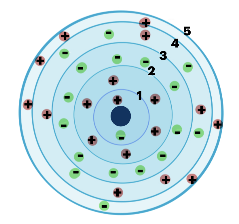
Figure 4: Local Margin

Mistake Budget	Label	$(c_{\text{low}},c_{\text{high}})$
$b=0$	None	$\emptyset$
$b=1,2,...,6$	$+$	$[\frac{1}{2},1)$
$b=7,8,...,10,11$	$-$	$[\frac{1}{3},\frac{1}{2})$
$b=12,13,...,16$	$-$	$[\frac{1}{4},\frac{1}{3})$
$b=17$	None	$\{\frac{1}{4}\}$
$b=18$	None	$\{0\}$

Figure 5: Guarantee for Figure 5.

It is easy to see the “simplest” classifier, $f^{*}$, that makes at most $b$ mistakes on $S^{\prime}$ has local margin (Definition 10) equal to the distance of the test point to the $b^{th}$ closest point with a different label. In other words, the local margin of the minimum complexity classifier, $f^{*}$, under the local margin complexity measure for the test point is $r$ as well. Our guarantee 5 is as follows: The learner outputs a label alongside a complexity interval. So long as the complexity of the target function belongs to the given interval and the adversary has corrupted at most $b$ of the training data points, our prediction is correct.

For instance, when there is no adversary, i.e., $b=0$, nearest neighbor classifier will abstain from prediction as the nearest positive and a negative train points have the same exact distance from the test point.

8.3.1 Proof of Theorem 5

Theorem 5. For any multi-class classification task, regularized robustly reliable learner, $\mathcal{L}$, (Definition 2) can be implemented efficiently for complexity measure Local Margin (Definition 9). Moreover, this learner is indeed the exact regularized-robustly-reliable (Definition 3).

Proof.

Given the training data $S^{\prime}$, the $(\mathcal{M},d_{\mathcal{M}})$ be a metric space, the test point $x_{test}$, and the mistake budget $b$, we are interested in the complexity of the classifiers with smallest local margin complexity with respect to the test point and its assigned labels, that make at most $b$ mistakes on $S^{\prime}$. First, we compute the distance of all training points from the yet unlabeled test point. For each class label, $y_{1},y_{2},...,y_{m}$ create a key in a dictionary and store the distances of all training points (from the test point) with labels opposite to the keys’, and sort the values of every key. In a $m$-class classification, there are $m$ keys and each key has at most $n$ entries. The learner starts by labeling the test point as $y_{1}$, and we check the $y_{1}$ key in our dictionary. The $b+1$’th value is the radius of the largest open ball we can draw around the test point labeled as $y_{1}$ such that it contains at most $b$ points with labels different from $y_{1}$. We denote this radius by $r_{1}$. The complexity of the least complex classifier that labels the test point as $y_{1}$ is $c_{y_{1}}=\frac{1}{r_{1}}$. We repeat this for all classes. Without loss of generality, assume $c_{y_{1}}\leq c_{y_{2}}\leq\dots\leq c_{y_{k}}$. We define:

$$c_{\text{low}}=c_{y_{1}},\quad c_{\text{high}}=c_{y_{2}}$$

where $c_{\text{low}}$ represents the minimum complexity value among the different labelings of $x_{\text{test}}$, and $c_{\text{high}}$ represents the second-lowest complexity value.

Finally, the predicted label for $x_{\text{test}}$ is determined as:

$$y=\underset{y_{1},y_{2},\dots,y_{m}}{\text{argmin}}\{c_{y_{1}},c_{y_{2}},\dots,c_{y_{m}}\}$$

That is, the label $y$ corresponding to the smallest complexity value is chosen. The learner then outputs the triplet $(y,c_{\text{low}},c_{\text{high}})$, where $y$ is the predicted label, $c_{\text{low}}$ is the lowest complexity value, and $c_{\text{high}}$ is the second-lowest complexity value, providing a guarantee on the prediction.

∎

8.4 Global Margin

Before proving Theorem 6, we first describe some useful properties of the global margin.

8.4.1 Understanding the Global Margin

Figure 6 shows the margin on one dimensional data. Let $S=\{(x,y)|x\in\mathcal{X},y\in\mathcal{Y}\}$ denote the set. Given a metric space $(\mathcal{M},d_{\mathcal{M}})$, draw the largest open ball, $B(x,r_{x})$ centered on every $x\in S$, such that for any $(x,y)\in S$, the ball $B(x,r_{x})$ does not contain any point $(x^{\prime},y^{\prime})$ from the set $S$ with label $y^{\prime}\neq y$. Each of these balls denote the (local) margin of their center point. The global margin of the set $S$ is the minimum over radius of such balls.

$$r_{S}=\underset{x\in S}{\min}\,\,r_{x}$$

We now prove the “simplest” classifier, $f^{*}$, that realizes set $S$ has global margin(Definition 10) of $\frac{r_{S}}{2}$. Moreover, the decision boundary of this classifier must be equidistant between the closest pairs of points with different labels. Hence, the decision boundary is placed midway between the closest points, and the global margin complexity of such function is $\frac{2}{r_{S}}$.

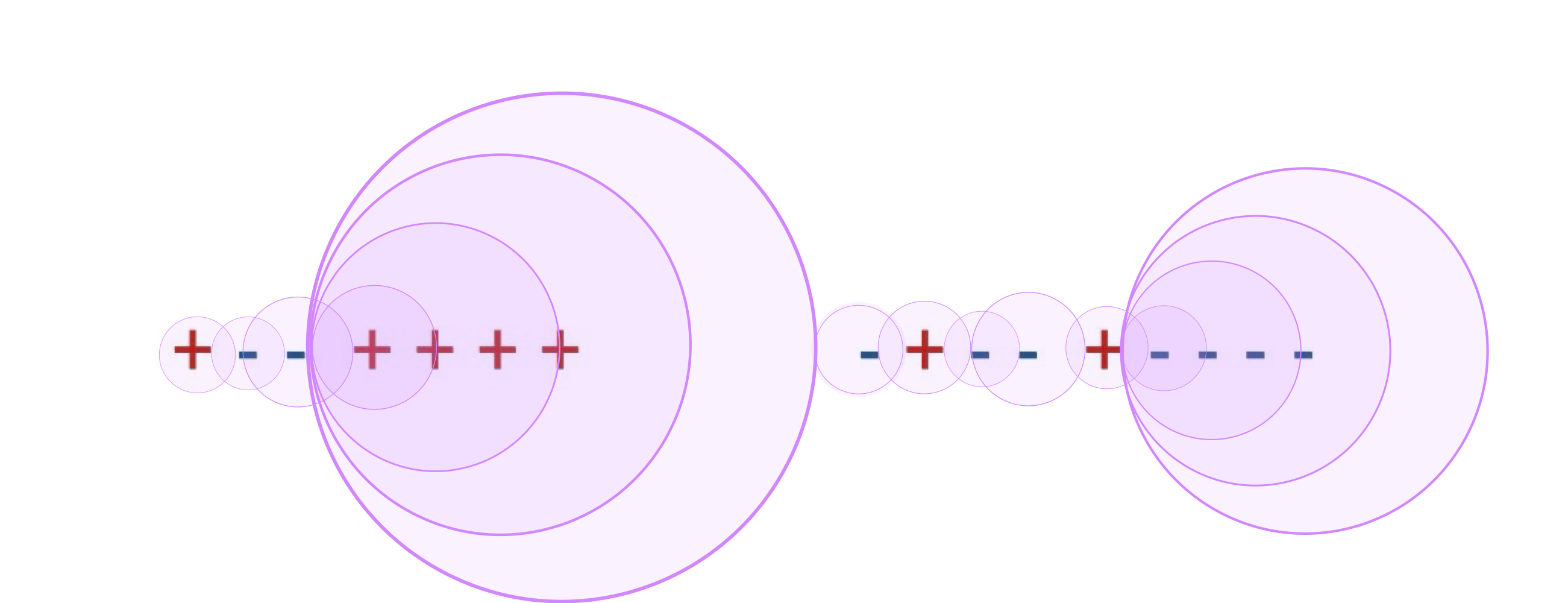
Figure 6: Global Margin on 1-dimensional data. Let $r_{S}$ be the radius of the smallest ball, and correspond to the distance between the closest pair of points with different labels. Then, the function with minimum global margin complexity with respect to this set is $\frac{2}{r_{S}}$ complex.

Theorem 9.

Let $(\mathcal{M},d_{\mathcal{M}})$ be a metric space, and $S=\{(x_{i},y_{i})\mid x_{i}\in\mathcal{X},\ y_{i}\in\mathcal{Y}\}$ be a finite set of labeled points, where $\mathcal{X}$ is the instance space and $\mathcal{Y}$ is the label space.

1. For each $x_{i}\in\mathcal{X}$, let $r_{i}$ be the minimum distance from $x_{i}$ to any point with a different label.

   $$r_{i}=\inf_{\begin{subarray}{c}x_{j}\in\mathcal{X}\\ y_{j}\neq y_{i}\end{subarray}}d_{\mathcal{M}}(x_{i},x_{j}),$$

2. Let $r_{S}$ denote the minimum distance between any two differently labeled points in $S$.

   $$r_{S}=\min_{x_{i}\in\mathcal{X}}r_{i}=\min_{\begin{subarray}{c}(x_{i},y_{i}),\ (x_{j},y_{j})\in S\\ y_{i}\neq y_{j}\end{subarray}}d_{\mathcal{M}}(x_{i},x_{j}),$$

Consider a classifier $f^{*}:\mathcal{X}\to\mathcal{Y}$ that realizes $S$, and obtains minimum global margin(Definition 10) complexity with respect to the set $S$. Then global margin (Definition 10) of $f^{*}$ is $\frac{2}{r_{S}}$. Moreover, its decision boundary $B_{f^{*}}$ is placed equidistantly between the closest pairs of points in $S$ with different labels.

Proof.

We first show that for any classifier $f^{*}$ that realizes $S$, the global margin $r$ cannot exceed $\frac{r_{S}}{2}$. Let $(x_{p},y_{p}),\ (x_{q},y_{q})\in S$ be a pair of points such that: $y_{p}\neq y_{q}$, and $d_{\mathcal{M}}(x_{p},x_{q})=r_{S}$. Since $r_{S}$ is the minimum distance between any two differently labeled points in $S$, such a pair exists. Consider any classifier $f^{*}$ that correctly classifies $S$. The minimum distance from $x_{p}$ (or $x_{q}$) to the decision boundary cannot exceed $\dfrac{r_{S}}{2}$. Formally, since $f^{*}$ must assign different labels to $x_{p}$ and $x_{q}$, there must exist a point $x_{b}\in B_{f^{*}}$ such that:

$$d_{\mathcal{M}}(x_{p},x_{b})+d_{\mathcal{M}}(x_{b},x_{q})=d_{\mathcal{M}}(x_{p},x_{q})=r_{S}.$$

By the triangle inequality, and because $x_{b}$ lies between $x_{p}$ and $x_{q}$, we have:

$$d_{\mathcal{M}}(x_{p},x_{b})=d_{\mathcal{M}}(x_{b},x_{q})\geq 0.$$

Since $d_{\mathcal{M}}(x_{p},x_{b})+d_{\mathcal{M}}(x_{b},x_{q})=r_{S}$, the maximal possible value for $d_{\mathcal{M}}(x_{p},x_{b})$ is $\frac{r_{S}}{2}$. Therefore, the minimum distance from any point in $S$ to the decision boundary $B_{f^{*}}$ satisfies:

$$r\leq\frac{r_{S}}{2}.$$

Now, we construct the classifier $f^{*}$ (which will just be the nearest-neighbor classifier) that realizes $S$ with a global margin $r=\frac{r_{S}}{2}$.

Let $f^{*}:\mathcal{X}\to\mathcal{Y}$ for any $x\in\mathcal{X}$ assign:

$$f^{*}(x)=\begin{cases}y_{i},&\text{if }d_{\mathcal{M}}(x,x_{i})<d_{\mathcal{M}}(x,x_{j})\text{ for all }x_{j}\in S\text{ with }y_{j}\neq y_{i},\\ y_{i}\text{ or }y_{j},&\text{if }d_{\mathcal{M}}(x,x_{i})=d_{\mathcal{M}}(x,x_{j})\text{ for some }x_{j}\in S,y_{j}\neq y_{i}.\end{cases}$$

This means, place the decision boundary $B_{f^{*}}$ equidistantly between all pairs $(x_{p},y_{p}),(x_{q},y_{q})\in S$ with $y_{p}\neq y_{q}$ and $d_{\mathcal{M}}(x_{p},x_{q})=r_{S}$. Since $f^{*}$ assigns to each $x_{i}\in S$ its correct label $y_{i}$, it correctly classifies $S$. We will now show that: $r_{f^{*}}\geq\frac{r_{S}}{2}$. Assume, for contradiction, that the global margin $r_{f^{*}}<\frac{r_{S}}{2}$. Then there exists $x_{i}\in S$ and $x_{b}\in B_{f^{*}}$ such that:

$$d_{\mathcal{M}}(x_{i},x_{b})=r-\epsilon<\dfrac{r_{S}}{2},$$

for some $\epsilon>0$. Since $x_{b}\in B_{f^{*}}$, there exists $x_{j}\in S$ with $y_{j}\neq y_{i}$ such that:

$$d_{\mathcal{M}}(x_{i},x_{b})=d_{\mathcal{M}}(x_{j},x_{b}).$$

Applying the triangle inequality:

$$d_{\mathcal{M}}(x_{i},x_{j})\leq d_{\mathcal{M}}(x_{i},x_{b})+d_{\mathcal{M}}(x_{b},x_{j})=2d_{\mathcal{M}}(x_{i},x_{b})<r_{S}.$$

Which contradicts the definition of $r_{S}$ as the minimum distance between differently labeled points in $S$. Therefore, our assumption is false, and we conclude that:

$$r_{f^{*}}\geq\frac{r_{S}}{2}.$$

Combining both directions we get

$$r_{f^{*}}=\frac{r_{S}}{2}.$$

∎

8.4.2 Proof of Theorem 6

Definition 14 (($c,r$)-Classification Graph).

Given $S=\{(x,y)|x\in\mathcal{X},y\in\mathcal{Y}\}$, where $\mathcal{X}$ denote the instance space and $\mathcal{Y}=\{1,2,...,c\}$ the label space, along with a metric space $(\mathcal{M},d_{\mathcal{M}})$, and complexity measure Global Margin (Definition 10), at every complexity level, $r$, we construct the ($c,r$)-Classification Graph, $\mathcal{G}_{r}$, by connecting every two points of different labels with distances less than $r$.

Remark 9.

The Minimum Vertex Cover of $\mathcal{G}_{r}$ corresponds to the smallest number of points that must be removed from $S$ so that a classifier achieves minimum global margin complexity (Definition 10) of $\frac{2}{r}$.

Using the remark above, we now prove Theorem 6.

Theorem 6. On a binary classification task, regularized robustly reliable learner, $\mathcal{L}$, (Definition 2) can be implemented efficiently for complexity measure Global Margin (Definition 10). Moreover, this learner is exact regularized-robustly-reliable (Definition 3).

Proof.

Algorithm 3 is the solution. We first compute the distance between every pair of training points, $S^{\prime}$, with opposite labels. Let $\mathcal{R}=\{0,r_{0},r_{1},...,r_{p}\}$ denote the set of aforementioned distances with an added zero. Without loss of generality, suppose $0\leq r_{0}\leq r_{1},...\leq r_{p}$. For the case of binary classification, the $(2,r)$-classification graph, $\mathcal{G}_{r}$, is bipartite. We construct each element, $(2,r)$-classification graph, of the set $\{\mathcal{G}_{r}(V^{+},V^{-},E_{r})\}_{r\in\mathcal{R}}$ by putting every positive training point in $V^{+}$, every negative training point in $V^{-}$, and connecting every two training points of opposite labels with distances less than $r$ by an edge, $e$, with capacity $c(e)$ corresponding to their distance. Since these graphs are bipartite, their Minimum Vertex Cover is the Maximum Matching Kőnig [1950] and can be computed efficiently. Notice that by increasing the radius, the Maximum Matching of classification graphs in the set only gets larger. Note that there is no edge in $\mathcal{G}_{0}$; hence the Matching is zero. We continue with computing the Maximum Matching of the classification graph with respect to the smallest radius, $\mathcal{G}_{r_{0}}$, which corresponds to the largest global margin complexity value. We continue to compute $\{\mathcal{G}_{r_{i}}\}_{r_{i}\in\mathcal{R}}$ in ascending order of $i$, and we stop as soon as we reach $p^{\prime}\in[0,p]$ such that the Maximum Matching of $\mathcal{G}_{r_{p^{\prime}}}$ is greater than $b$, the mistake budget. Next, when the test point $x_{\text{test}}$ arrives, the learner begins by assigning it a negative label. We compute the distance of the test point, $x_{test}$ from every positive training point. We run a binary search on the possible values of radius, i.e., $[0,p^{\prime}]$. At every level $r_{i}$, We denote the set of training points labeled as positive with distance $r_{test}$ that $r_{i}\leq r_{test}<r_{i+1}$ from $x_{\text{test}}$ by $\bar{V}_{r_{test}}^{+}$. We denote the cardinality of $\bar{V}_{r_{test}}^{+}$ by $\delta_{r_{test}}$, which is indeed the degree of $x_{\text{test}}$ at complexity level $r_{test}$. If $\delta_{r_{test}}$ exceeds our mistake budget, $b$, we break and move to a smaller radius (higher complexity). Otherwise, we add $\delta_{r_{test}}$ copies of the test point and connect each of which to a distinct point in $\bar{V}_{r_{test}}^{+}$. We denote the set of $\delta_{r_{test}}$ newly added edges by $\bar{E}_{r_{test}}$. We have constructed a new graph $\mathcal{G}_{r_{test}}=\mathcal{G}_{r_{i}}(V^{+},V^{-}\cup\{x_{{test}_{i}}\}_{i\in[1,\delta_{r_{test}}]},E_{r_{i}}\cup\bar{E}_{r_{test}})$, which ensures all the points adjacent to $x_{test}$ are contained in the Minimum Vertex Cover. We can compute the the Maximum Matching of $\mathcal{G}_{{r_{test}}}$ in $\mathcal{O}(\delta_{r_{test}}.(\delta_{r_{test}}+|E|))$ by updating the Maximum Matching of $\mathcal{G}_{r_{i}}$. If Maximum Matching at the current complexity level exceeds the poisoning budget, $b$, we should move to a smaller radius (higher complexity), and if it is less than or equal to our mistake budget, $b$, we search to see if the condition still holds for a larger radius. We accordingly use the corresponding pre-computed representation graphs of the new complexity level. We do the same thing for the test point labeled as positive. Finally, $c_{\text{low}}=\min\{\frac{2}{r_{\text{max}}^{+}},\frac{2}{r_{\text{max}}^{-}}\}$, and $c_{\text{high}}=\max\{\frac{2}{r_{\text{max}}^{+}},\frac{2}{r_{\text{max}}^{-}}\}$. We output $y_{\text{test}}=\underset{+,-}{\text{argmin}}\{\frac{2}{r_{\text{max}}^{+}},\frac{2}{r_{\text{max}}^{-}}\}$, along with $c_{\text{low}},c_{\text{high}}$. ∎

Input: $S^{\prime}=\{(x,y)\}$, metric $\mathcal{M}$, Mistake budget $b$

for every $(x,y),(x^{\prime},y^{\prime})\in S^{\prime}$ with $y\neq y^{\prime}$ do

       Compute $d_{\mathcal{M}}(x,x^{\prime})$;

      

end for

Store the sorted distances and zero in $\mathcal{R}_{train}=\{0,r_{0},r_{1},\dots,r_{p_{train}}\}$

Initialize $r\leftarrow 0$, $p^{\prime}\leftarrow p_{train}$

while $r\leq p_{train}$ do

       for each $\mathcal{G}_{r}(V^{+},V^{-},E_{r})$ where $r\in\mathcal{R}_{train}$ do

             $V^{+}\leftarrow\{x\mid(x,y)\in S^{\prime},\;y=\textbf{'+'}\}$

             $V^{-}\leftarrow\{x\mid(x,y)\in S^{\prime},\;y=\textbf{'-'}\}$

             $E_{r}\leftarrow\{e(u,v)\mid u\in V^{+},v\in V^{-},d_{\mathcal{M}}(u,v)<r$ with $c(e)=d_{\mathcal{M}}(u,v)$}

            

       end for

      Compute $\textbf{MaxMatch}(\mathcal{G}_{r})$

       if $\textbf{MaxMatch}(\mathcal{G}_{r})>b$ then

             $p^{\prime}\leftarrow r-1$

             break;

            

       end if

      $r\leftarrow r+1$;

      

end while

return $\{\mathcal{G}_{r}(V^{+},V^{-},E_{r})\}_{r\in[0,p^{\prime}]}$ ;

Algorithm 2 Global Margin (Definition 10) Learner Precomputing

Input: $x_{\text{test}}$: Test point, $S$: Train set, $b$: Mistake budget, $\{\mathcal{G}_{r}(V^{+},V^{-},E_{r})\}_{r\in[0,p^{\prime}]}$

Output: Test label and the guarantee

$left\leftarrow 0$, $right\leftarrow|\{\mathcal{G}_{r}(V^{+},V^{-},E_{r})\}_{r\in[0,p^{\prime}]}|$;

if $y_{\text{test}}=\textbf{'-'}$ then

       Initialize $\mathcal{R}_{test}\leftarrow\emptyset$

       for each $(x,y)\in S^{\prime}$ with $y=\textbf{'+'}$ do

             Add $d_{\mathcal{M}}(x,x_{\text{test}})$ to $\mathcal{R}_{test}$;

            

      Sort($\mathcal{R}_{test}$)

       while left $\leq right$ do

             $current\leftarrow left+\lfloor(right-left)/2\rfloor$

             for $r_{\text{test}}$ in $\mathcal{R}_{test}$ do

                   if $r_{\text{current}}\leq r_{\text{test}}<r_{\text{current+1}}$ then

                         $\bar{V}_{r_{\text{test}}}^{+}\leftarrow\{v\in V^{+}(\mathcal{G}_{r_{\text{current}}})\mid\text{dist}(v,x_{\text{test}})<r_{\text{test}}\}$

                         $\delta_{r_{\text{test}}}\leftarrow|\bar{V}_{r_{\text{test}}}^{+}|$;

                        

                        if $\delta_{r_{\text{test}}}>b$ then

                               $right\leftarrow current-1$

                               break;

                              

                        else

                               $V_{r_{\text{test}}}^{-}\leftarrow V^{-}\cup\{x_{\text{test}_{i}}\}_{i\in[\delta_{r_{\text{test}}}]}$

                               $E_{r_{\text{test}}}\leftarrow E_{r_{\text{current}}}\cup\{e_{i}=(x_{\text{test}_{i}},\bar{V}_{r_{\text{test}}}^{+}[i]),c(e_{i})=d_{\mathcal{M}}(x_{\text{test}},\bar{V}_{r_{\text{test}}}^{+}[i])\}_{i\in[\delta_{r_{\text{test}}}]}$

                               $b_{r_{\text{test}}}^{-}\leftarrow\textbf{MaxMatch}(V^{+},V_{r_{\text{test}}}^{-},E_{r_{\text{test}}})$;

                              

                              if $b_{r_{\text{test}}}^{-}\leq b$ then

                                     $r_{\text{max}}^{-}\leftarrow r_{\text{test}}$

                                     $left\leftarrow current+1$;

                                    

                              else

                                     $right\leftarrow current-1$

                                     break;

                                    

                              

                        

                  else

                         $r_{\text{max}}^{-}\leftarrow r_{current}$

                         $left\leftarrow current+1$

                  

            

      

Repeat the same for $y_{\text{test}}=\textbf{'+'}$;

return $\left(\frac{2}{r_{\text{max}}^{+}},\frac{2}{r_{\text{max}}^{-}}\right)$;

Algorithm 3 Global Margin (Definition 10) Learner

8.4.3 Proof of Theorem 7

Definition 15 (K-Regular Graph).

A graph is said to be $K$-regular if its every vertex has degree $K$.

Theorem 7. For any multi-class classification task with three or more classes, implementing regularized robustly reliable learner, $\mathcal{L}$, (Definition 2) for complexity measure Global Margin (Definition 10) is NP-hard, and can be done efficiently with access to ECM oracle (Definition 1).

Proof.

We aim to show that finding the minimum Vertex Cover of a $(k,r)$-representation graph $\mathcal{G}_{(r)}$, for $k\geq 3$ is NP-hard. It is known that finding the Vertex Cover on cubic graphs is APX-Hard, Alimonti and Kann [2000]. Moreover, by Brooks’ theorem Gotti [2018], Bona [2016], it is known that a 3-regular graph that is neither complete nor an odd cycle has a chromatic number of 3, meaning that there exists a 3-coloring for such a graph. We now demonstrate that finding the minimum Vertex Cover for any $k$-colored 3-regular graph, where the graph is neither complete nor an odd cycle, can be reduced in polynomial time to the problem of finding the minimum Vertex Cover of a $(k,r)$-classification graph. This reduction is accomplished by embedding the vertices of the 3-regular graph into the edge space $\mathbb{R}^{m}$, where $m=|E|$, the number of edges in the graph. For each vertex $v\in V$, we construct its embedding as follows: if edge $e_{i}$ is incident to vertex $v$, then the $i$’th dimension of $v$’s embedding is set to 1; otherwise, it is set to 0. Since the graph is 3-regular, each vertex embedding contains exactly three entries of 1, corresponding to the edges incident to that vertex.

The Hamming distance between two vertices in this embedding space encodes adjacency information. Specifically, if two vertices $v_{1}$ and $v_{2}$ are adjacent in the graph, their Hamming distance in the embedding space is 4; if they are not adjacent, their distance is 6. This embedding provides a direct correspondence between the adjacency relations in the original graph and the structure of the $(k,r)$-classification graph. Thus, any $k$-colored 3-regular graph can be reduced to a $(k,r)$-classification graph in polynomial time. Given that the Vertex Cover problem is hard for $K$-regular graphs, and this reduction preserves the structural properties of the graph, it follows that finding the minimum Vertex Cover in a $(k,r)$-classification graph is also hard. Therefore, implementing the learner $\mathcal{L}$ is NP-hard, completing the proof.

With ECM Oracle (Definition 1) Access: Let $S^{\prime}$ represent the corrupted training set. To evaluate the test point $x_{\text{test}}$ with label $y_{\text{test}}$, we proceed as follows. First, we augment $S^{\prime}$ by adding $b+1$ copies of $x_{\text{test}}$ each labeled as $y_{\text{test}}=y_{1}$. This ensures that the mistake budget of the ECM algorithm is not depleted by the test point $x_{\text{test}}$, as the additional copies force the algorithm to allocate its mistake budget elsewhere.

We then run the ECM algorithm on this modified dataset, and denote the complexity returned by the oracle as $c_{y_{1}}$. Next, we repeat this procedure for the remaining possible labels $y_{2},\dots,y_{m}$, each time augmenting the dataset with $b+1$ copies of $x_{\text{test}}$ labeled according to $y_{i}$. Let the corresponding complexities returned by the ECM oracle be denoted as $c_{y_{2}},\dots,c_{y_{k}}$. Without loss of generality, assume $c_{y_{1}}\leq c_{y_{2}}\leq\dots\leq c_{y_{k}}$ We define:

$$c_{\text{low}}=c_{y_{1}},\quad c_{\text{high}}=c_{y_{2}}$$

where $c_{\text{low}}$ represents the minimum complexity value among the different labelings of $x_{\text{test}}$, and $c_{\text{high}}$ represents the second-lowest complexity value.

Finally, the predicted label for $x_{\text{test}}$ is determined as:

$$y=\underset{y_{1},y_{2},\dots,y_{k}}{\text{argmin}}\{c_{y_{1}},c_{y_{2}},\dots,c_{y_{k}}\}$$

That is, the label $y$ corresponding to the smallest complexity value is chosen. The learner then outputs the triplet $(y,c_{\text{low}},c_{\text{high}})$, where $y$ is the predicted label, $c_{\text{low}}$ is the lowest complexity value, and $c_{\text{high}}$ is the second-lowest complexity value, providing a guarantee on the prediction.

∎

Example 3.

We now aim to demonstrate why such a reduction to the edge space is necessary, and to clarify that not all 3-regular graphs, which are neither complete nor odd cycles, inherently belong to the class of $(k,r)$-Classification Graphs within their original metric space. Consider the well-known Petersen graph, which is a 3-regular and is neither complete nor an odd cycle; hence is 3-colorable. While it satisfies the structural properties for 3-colorability, the graph does not behave as a 3-classification graph when embedded in $\mathbb{R}^{2}$. Specifically, the metric space properties are not satisfied.

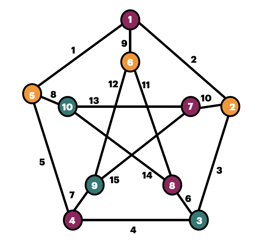
Figure 7: Petersen Graph

For example, the vertices $v_{6}$ and $v_{10}$ are closer to each other than the vertices $v_{6}$ and $v_{9}$, yet vertices $v_{6}$ and $v_{10}$ are not connected in the original graph, violating the requirements of a classification graph in its natural embedding. This example highlights that the geometric constraints imposed by the original metric space are too restrictive for certain 3-regular graphs to be used directly as $(k,r)$-classification graphs. To resolve this issue, we embed the vertices of the Petersen graph into the edge space, $\mathbb{R}^{m}$, where $m=|E|$ is the number of edges in the graph.

• $v_{1}:[1,1,0,0,0,0,0,0,1,0,0,0,0,0,0]$,

• $v_{2}:[0,1,1,0,0,0,0,0,0,1,0,0,0,0,0]$,

• $v_{3}:[0,0,1,1,0,1,0,0,0,0,0,0,0,0,0]$,

• $v_{4}:[0,0,0,1,1,0,1,0,0,0,0,0,0,0,0]$,

• $v_{5}:[1,0,0,0,1,0,0,1,0,0,0,0,0,0,0]$,

• $v_{6}:[0,0,0,0,0,0,0,0,1,0,1,1,0,0,0]$,

• $v_{7}:[0,0,0,0,0,0,0,0,0,1,1,0,0,0,1]$,

• $v_{8}:[0,0,0,0,0,1,0,0,0,0,0,0,0,1,1]$,

• $v_{9}:[0,0,0,0,0,0,1,0,0,0,0,0,1,1,0]$,

• $v_{10}:[0,0,0,0,0,0,0,1,0,0,0,1,1,0,0]$.

This transformation ensures that the embeddings satisfy the metric space properties required for classification graphs since it preserves the required distance properties for classification: two adjacent vertices in the Petersen graph, such as $v_{6}$ and $v_{9}$, have a Hamming distance of 4, while non-adjacent vertices such as $v_{6}$ and $v_{10}$ have a distance of 6. By embedding the graph into the edge space, we transform it into a $(k,r)$-classification graph that respects the desired metric space properties.

8.5 Degree of Polynomial

8.5.1 Proof of theorem 8

Theorem 8. On a binary classification task, regularized robustly reliable learner, $\mathcal{L}$, (Definition 2) can be implemented efficiently using ECM oracle (Definition 1) for complexity measure Degree of Polynomial (Definition 13). Moreover, the learner is exact regularized-robustly-reliable (Definition 3).

Proof.

Given a corrupted training set $S^{\prime}$, and a mistake budget $b$, we first run the ECM algorithm on the training set $S^{\prime}$, which outputs a classifier $h_{S^{\prime}}$ that minimizes the complexity while making at most $b$ mistakes on $S^{\prime}$. Let the complexity of $h_{S^{\prime}}$ be denoted by $c_{\text{low}}=\mathcal{C}(h_{S^{\prime}})$. The classifier $h_{S^{\prime}}$ is the minimum complexity classifier among all hypotheses that make no more than $b$ mistakes on $S^{\prime}$. Using the classifier $h_{S^{\prime}}$, we label the test point $x_{\text{test}}$, i.e., $y=h_{S^{\prime}}(x_{\text{test}})$. We modify the training set by adding $b+1$ copies of the test point $x_{\text{test}}$, but with the label opposite to $y$, i.e., the added points have label $\neg y$. Let this modified set be denoted as $S^{\prime\prime}$. The addition of $b+1$ copies of $x_{\text{test}}$ ensures that any classifier produced by ECM will be forced to change the label of $x_{\text{test}}$ if it is to remain within the mistake budget. We now run ECM on the modified training set $S^{\prime\prime}$, which outputs a new classifier. The complexity of this new classifier is denoted by $c_{\text{high}}$. Since the classifier now labels $x_{\text{test}}$ as $\neg y$, the complexity $c_{\text{high}}$ represents the minimum complexity required to label $x_{\text{test}}$ differently from $h_{S^{\prime}}(x_{\text{test}})$. By construction, $c_{\text{high}}$ must be greater than or equal to $c_{\text{low}}$ due to the added complexity of labeling the test point differently. Finally, we output the triple $(y,c_{\text{low}},c_{\text{high}})$ as our guarantee.

∎

8.6 Interval Probability Mass

Definition 16 (Label Noise Biggio et al. [2011] Adversary).

Label noise was formally introduced in Biggio et al. [2011]. Consider the set of original points $S=\{\{(x_{i},y_{i})\}_{i=1}^{n}|x\in\mathcal{X},y\in\mathcal{Y}\}$, where $\mathcal{X}$ denote the instance space and $\mathcal{Y}$ the label space. Concretely, given a mistake budget $b$, the label noise adversary is allowed to alter the labels of at most $b$ points in the dataset $S$. That is, the Hamming distance between the original labels $S$ and the modified labels $S^{\prime}$, denoted by $d_{H}(S,S^{\prime})$, must satisfy the constraint:

$$d_{H}(S,S^{\prime})=\sum_{i=1}^{n}\textbf{1}(y_{i}\neq y_{i}^{\prime}\mid x_{i}=x_{i}^{\prime})\leq b.$$

Let $\mathcal{A}(S)$ denote the sample corrupted by adversary $\mathcal{A}$. For a mistake budget $b$, let $\mathcal{A}_{b}$ be the set of adversaries with corruption budget $b$ and $\mathcal{A}_{b}(S)=\{S^{\prime}\mid d(S,S^{\prime})\leq b\}$ denote the possible corrupted training samples under an attack from an adversary in $\mathcal{A}_{b}$. Intuitively, if the given sample is $S^{\prime}$, we would like to give guarantees for learning when $S^{\prime}\in\mathcal{A}_{b}$ for some (realizable) un-corrupted sample $S$.

Theorem 10.

For the binary classification task, regularized robustly reliable learner, $\mathcal{L}$, (Definition 2) can be implemented efficiently for complexity measure Interval Probability Mass (Definition 12) with the label noise adversary (Definition 16). Moreover, the learner is exact regularized-robustly-reliable (Definition 3).

Proof.

First, we define the DPs that store the scores used, then we use the DP table to compute the complexity level when the test point and mistake budget arrive. We define $DP+,DP-,DP^{\prime}+,DP^{\prime}-$ each of which are 3D tables of size $n\times(n+1)\times n$. The first dimension denote the position of the current data point, namely for $DP+$ and $DP-$, we denote the rightmost point by index 0, and the leftmost point by index $n-1$. As for $DP^{\prime}+$ and $DP^{\prime}-$, the first dimension denote the position of the current data point in the reverse sequence, i.e., we denote the rightmost point by index $n-1$, and the leftmost point by index $0$. The second dimension denote the number of mistakes made up to the current point, which can vary between $0$ to the number of points so far. Lastly, the third dimension denote the starting point of the interval containing the current point, denoted by the first dimension. We provide the proof of correctness for $DP+$, and it is similar for the other three.

Base Case Consider $i=0$ (the first point in the sequence): Initialize the entire table to infinity.

• If $a[0]=\texttt{'+'}$:

  • We initialize $DP_{+}[0][0][0]=\frac{n}{2}$ because the complexity is $\frac{n}{2}$ with no mistakes made, and the rightmost point is positive.

• If $a[0]=\texttt{'-'}$:

  • We set $DP_{+}[0][1][0]=\frac{n}{2}$, as we can use the mistake budget and flip the negative label to a positive.

Inductive Hypothesis: Assume that for all positions up to $i-1$, the table DP_+[$i-1$][$j$][$k$] correctly stores the minimum complexity score for all possible configurations of mistakes and interval boundaries.

Inductive Step: We will show that the table DP_+[$i$][$j$][$k$] correctly computes the minimum complexity score at position $i$, based on the following cases:

• Case 1: $a[i]=\texttt{'-'}$

  • if $k=i-1$: DP_+ requires the $i$’th point to be a positive; thus, this point must be removed. We need to decrement the mistake count $j$ of the $i-1$’th point by one and use it to remove this point. Note that the $i-1$ must be a negative point in order to have $k=i-1$.

    $$\text{{DP\_+[$i$][$j$][$k$]}}=\min_{k^{\prime},j^{\prime}\in[0,j-1]}(\text{{DP\_-[$i-1$][$j^{\prime}$][$k^{\prime}$]}})+\frac{n}{2}$$

  • if $k<i-1$: Then we flip the label of this point, and update the total score.

    $$\text{{DP\_+[$i$][$j$][$k$]}}=\min_{j^{\prime}\in[0,j-1]}\text{{DP\_+[$i-1$][$j^{\prime}$][$k$]}}-\frac{n}{i-k+1}+\frac{n}{i-k+2}$$

• Case 2: $a[i]=\texttt{'+'}$

  • if $k=i-1$: The $i-1$ must be a negative point in order to have $k=i-1$.

    $$\text{{DP\_+[$i$][$j$][$k$]}}=\min_{k^{\prime},j^{\prime}\in[0,j]}(\text{{DP\_-[$i-1$][$j^{\prime}$][$k^{\prime}$]}})+\frac{n}{2}$$

  • if $k<i-1$: Then we update the total score.

    $$\text{{DP\_+[$i$][$j$][$k$]}}=\min_{j^{\prime}\in[0,j]}\text{{DP\_+[$i-1$][$j^{\prime}$][$k$]}}-\frac{n}{i-k+1}+\frac{n}{i-k+2}$$

Thus, the DP algorithm correctly computes the complexity measure as defined, proving its correctness for DP_+.

Computing the test label efficiently: We now use the DP tables to obtain the test label. Note that our approach does not require re-training to compute the test label efficiently. Once we receive the test point’s position along with adversary’s budget, $b$, we compute the exact minimum complexity needed to label it point as positive and negative. We denote the test point’s position by $test\_pos$, there are four different formations for the label of test point’s right most and left most neighbor. Given $b$, we iterate over all possible divisions of mistake budget, as well as the position of the starting point of the previous intervals from the left and the right side of the test point in each of these four formations. Define the minimum complexity to label the test point as positive, $c_{+}$ and the minimum complexity to label the test point as negative, $c_{-}$. Then, $c_{\text{low}}=\min\{c_{+},c_{-}\}$, and $c_{\text{high}}=\max\{c_{+},c_{-}\}$. We output $y=\underset{+,-}{\text{argmin}}\{c_{+},c_{-}\}$, along with $c_{\text{low}},c_{\text{high}}$. ∎

Remark 10.

Theorem 10 can be generalized to classification tasks with more than two classes.

Input: $a$: Train set

Output: $DP_{+}$, $DP_{-}$, $DP^{\prime}_{+}$, $DP^{\prime}_{-}$

for $i=1$ to $n$ do

       for $j=0$ to $i+2$ do

             for $k=0$ to $i+1$ do

                   if $a[i]$ is ’+’ then

                         if $k==i$ then

                               $DP_{+}[i][j][k]\leftarrow\min_{k^{\prime},j^{\prime}\in[0,j]}(DP_{-}[i-1][j^{\prime}][k^{\prime}])+\frac{n}{2}$

                               $DP_{-}[i][j][k]\leftarrow\min_{k^{\prime},j^{\prime}\in[0,j]-1}(DP_{+}[i-1][j^{\prime}][k^{\prime}])+\frac{n}{2}$;

                              

                        else

                               $DP_{+}[i][j][k]\leftarrow\min_{j^{\prime}\in[0,j]}DP_{+}[i-1][j^{\prime}][k]-\frac{n}{i-k+1}+\frac{n}{i-k+2}$

                               $DP_{-}[i][j][k]\leftarrow\min_{j^{\prime}\in[0,j-1]}DP_{-}[i-1][j^{\prime}][k]-\frac{n}{i-k+1}+\frac{n}{i-k+2}$;

                              

                         end if

                        

                   end if

                  if $a[i]$ is ’-’ then

                         if $k==i$ then

                               $DP_{+}[i][j][k]\leftarrow\min_{k^{\prime},j^{\prime}\in[0,j-1]}(DP_{-}[i-1][j^{\prime}][k^{\prime}])+\frac{n}{2}$

                               $DP_{-}[i][j][k]\leftarrow\min_{k^{\prime},j^{\prime}\in[0,j]}(DP_{+}[i-1][j^{\prime}][k^{\prime}])+\frac{n}{2}$;

                              

                        else

                               $DP_{+}[i][j][k]\leftarrow\min_{j^{\prime}\in[0,j-1]}DP_{+}[i-1][j^{\prime}][k]-\frac{n}{i-k+1}+\frac{n}{i-k+2}$

                               $DP_{-}[i][j][k]\leftarrow\min_{j^{\prime}\in[0,j]}DP_{-}[i-1][j^{\prime}][k]-\frac{n}{i-k+1}+\frac{n}{i-k+2}$;

                              

                         end if

                        

                   end if

                  

                  if $a\_reversed[i]$ is ’+’ then

                         if $k==i$ then

                               $DP^{\prime}_{+}[i][j][k]\leftarrow\min_{k^{\prime},j^{\prime}\in[0,j]}(DP^{\prime}_{-}[i-1][j^{\prime}][k^{\prime}])+\frac{n}{2}$

                               $DP^{\prime}_{-}[i][j][k]\leftarrow\min_{k^{\prime},j^{\prime}\in[0,j-1]}(DP^{\prime}_{+}[i-1][j^{\prime}][k^{\prime}])+\frac{n}{2}$;

                              

                        else

                               $DP^{\prime}_{+}[i][j][k]\leftarrow\min_{j^{\prime}\in[0,j]}DP^{\prime}_{+}[i-1][j^{\prime}][k]-\frac{n}{i-k+1}+\frac{n}{i-k+2}$

                               $DP^{\prime}_{-}[i][j][k]\leftarrow\min_{j^{\prime}\in[0,j-1]}DP^{\prime}_{-}[i-1][j^{\prime}][k]-\frac{n}{i-k+1}+\frac{n}{i-k+2}$;

                              

                         end if

                        

                   end if

                  if $a\_reversed[i]$ is ’-’ then

                         if $k==i$ then

                               $DP^{\prime}_{+}[i][j][k]\leftarrow\min_{k^{\prime},j^{\prime}\in[0,j-1]}(DP^{\prime}_{-}[i-1][j^{\prime}][k^{\prime}])+\frac{n}{2}$

                               $DP^{\prime}_{-}[i][j][k]\leftarrow\min_{k^{\prime},j^{\prime}\in[0,j]}(DP^{\prime}_{+}[i-1][j^{\prime}][k^{\prime}])+\frac{n}{2}$;

                              

                        else

                               $DP^{\prime}_{+}[i][j][k]\leftarrow\min_{j^{\prime}\in[0,j-1]}DP^{\prime}_{+}[i-1][j^{\prime}][k]-\frac{n}{i-k+1}+\frac{n}{i-k+2}$

                               $DP^{\prime}_{-}[i][j][k]\leftarrow\min_{j^{\prime}\in[0,j]}DP^{\prime}_{-}[i-1][j^{\prime}][k]-\frac{n}{i-k+1}+\frac{n}{i-k+2}$;

                              

                         end if

                        

                  else

                        

                   end if

                  

             end for

            

       end for

      

end for

return $DP_{+}$, $DP_{-}$, $DP^{\prime}_{+}$, $DP^{\prime}_{-}$;

Algorithm 4 DP Score of Interval Probability Mass 10 with Label Noise 16

References

- Alimonti and Kann [2000] Paola Alimonti and Viggo Kann. Some apx-completeness results for cubic graphs. Theoretical Computer Science, 237(1):123–134, 2000. ISSN 0304-3975. doi: https://doi.org/10.1016/S0304-3975(98)00158-3. URL https://www.sciencedirect.com/science/article/pii/S0304397598001583.
- Awasthi et al. [2018] Pranjal Awasthi, Maria Florina Balcan, and Philip M. Long. The power of localization for efficiently learning linear separators with noise, 2018. URL https://arxiv.org/abs/1307.8371.
- Balcan et al. [2022] Maria-Florina Balcan, Avrim Blum, Steve Hanneke, and Dravyansh Sharma. Robustly-reliable learners under poisoning attacks. In Conference on Learning Theory, pages 4498–4534. PMLR, 2022.
- Barreno et al. [2006] Marco Barreno, Blaine Nelson, Russell Sears, Anthony D. Joseph, and J. D. Tygar. Can machine learning be secure? In Proceedings of the 2006 ACM Symposium on Information, Computer and Communications Security, ASIACCS ’06, page 16–25, New York, NY, USA, 2006. Association for Computing Machinery. ISBN 1595932720. doi: 10.1145/1128817.1128824. URL https://doi.org/10.1145/1128817.1128824.
- Biggio et al. [2011] Battista Biggio, Blaine Nelson, and Pavel Laskov. Support vector machines under adversarial label noise. In Chun-Nan Hsu and Wee Sun Lee, editors, Proceedings of the Asian Conference on Machine Learning, volume 20 of Proceedings of Machine Learning Research, pages 97–112, South Garden Hotels and Resorts, Taoyuan, Taiwain, 14–15 Nov 2011. PMLR. URL https://proceedings.mlr.press/v20/biggio11.html.
- Bona [2016] M. Bona. Walk Through Combinatorics, A: An Introduction To Enumeration And Graph Theory (Fourth Edition). World Scientific Publishing Company, 2016. ISBN 9789813148864. URL https://books.google.com/books?id=uZRIDQAAQBAJ.
- Bosek et al. [2014] Bartlomiej Bosek, Dariusz Leniowski, Piotr Sankowski, and Anna Zych. Online bipartite matching in offline time. In 2014 IEEE 55th Annual Symposium on Foundations of Computer Science, pages 384–393, 2014. doi: 10.1109/FOCS.2014.48.
- Bshouty et al. [2002] Nader H. Bshouty, Nadav Eiron, and Eyal Kushilevitz. Pac learning with nasty noise. Theoretical Computer Science, 288(2):255–275, 2002. ISSN 0304-3975. doi: https://doi.org/10.1016/S0304-3975(01)00403-0. URL https://www.sciencedirect.com/science/article/pii/S0304397501004030. Algorithmic Learning Theory.
- Chen et al. [2017] Xinyun Chen, Chang Liu, Bo Li, Kimberly Lu, and Dawn Song. Targeted backdoor attacks on deep learning systems using data poisoning, 2017. URL https://arxiv.org/abs/1712.05526.
- El-Yaniv and Wiener [2010] Ran El-Yaniv and Yair Wiener. On the foundations of noise-free selective classification. Journal of Machine Learning Research, 11(53):1605–1641, 2010. URL http://jmlr.org/papers/v11/el-yaniv10a.html.
- Gao et al. [2021] Ji Gao, Amin Karbasi, and Mohammad Mahmoody. Learning and certification under instance-targeted poisoning, 2021. URL https://arxiv.org/abs/2105.08709.
- Geiping et al. [2021] Jonas Geiping, Liam Fowl, W. Ronny Huang, Wojciech Czaja, Gavin Taylor, Michael Moeller, and Tom Goldstein. Witches’ brew: Industrial scale data poisoning via gradient matching, 2021. URL https://arxiv.org/abs/2009.02276.
- Gotti [2018] Federico Gotti. Brooks’ theorem, 2018. URL https://math.mit.edu/~fgotti/docs/Courses/Combinatorial%20Analysis/32.%20Brooks%27%20Theorem/Brooks%27%20Theorem.pdf. Accessed: 2024-07-03.
- Kearns and Li [1993] Michael Kearns and Ming Li. Learning in the presence of malicious errors. SIAM Journal on Computing, 22(4):807–837, 1993. doi: 10.1137/0222052. URL https://doi.org/10.1137/0222052.
- Klivans et al. [2009] Adam Klivans, Philip Long, and Rocco Servedio. Learning halfspaces with malicious noise. volume 10, pages 2715–2740, 12 2009. ISBN 978-3-642-02926-4. doi: 10.1007/978-3-642-02927-1˙51.
- Kőnig [1950] Dénes Kőnig. Theory of Finite and Infinite Graphs. Birkhäuser, Boston, 1950. English translation of the original 1931 German edition.
- Levine and Feizi [2021] Alexander Levine and Soheil Feizi. Deep partition aggregation: Provable defense against general poisoning attacks, 2021. URL https://arxiv.org/abs/2006.14768.
- Mozaffari-Kermani et al. [2015] Mehran Mozaffari-Kermani, Susmita Sur-Kolay, Anand Raghunathan, and Niraj K. Jha. Systematic poisoning attacks on and defenses for machine learning in healthcare. IEEE Journal of Biomedical and Health Informatics, 19(6):1893–1905, 2015. doi: 10.1109/JBHI.2014.2344095.
- Rivest and Sloan [1988] Ronald L Rivest and Robert H Sloan. Learning complicated concepts reliably and usefully. In Proceedings of the Association for the Advancement of Artificial Intelligence (AAAI), pages 635–640, 1988.
- Shafahi et al. [2018] Ali Shafahi, W. Ronny Huang, Mahyar Najibi, Octavian Suciu, Christoph Studer, Tudor Dumitras, and Tom Goldstein. Poison frogs! targeted clean-label poisoning attacks on neural networks, 2018. URL https://arxiv.org/abs/1804.00792.
- Suciu et al. [2018] Octavian Suciu, Radu Marginean, Yigitcan Kaya, Hal Daume III, and Tudor Dumitras. When does machine learning FAIL? generalized transferability for evasion and poisoning attacks. In 27th USENIX Security Symposium (USENIX Security 18), pages 1299–1316, Baltimore, MD, August 2018. USENIX Association. ISBN 978-1-939133-04-5. URL https://www.usenix.org/conference/usenixsecurity18/presentation/suciu.
- Valiant [1985] Leslie G Valiant. Learning disjunctions of conjunctions. In Proceedings of the 9th International Joint Conference on Artificial Intelligence, pages 560–566, 1985.