A Multi-Dimensional Mathematical Model for Surface Exerted Point Forces in Elastic Media

Sabia Asghara,b,111Corresponding author: Sabia Asghar E-mail address: sabia.asghar@uhasselt.be, Qiyao Pengc,d and Fred Vermolena,b,e,f

aDepartment of Mathematics and Statistics, Computational Mathematics Group, University of Hasselt, Diepenbeek, Belgium

bData Science Institute (DSI), University of Hasselt, Diepenbeek, Belgium

cMathematical Institute, Leiden University, Leiden, The Netherlands

dBioinformatics, Department of Computer Science, Vrije Universiteit Amsterdam, Amsterdam, The Netherlands

eDepartment of Mathematics and Applied Mathematics, University of Johannesburg, Johannesburg, South Africa

fDelft Institute of Applied Mathematics, Delft University of Technology, Mekelweg 4, 2628 CD Delft, The Netherlands

Abstract: Some phenotypes of biological cells exert mechanical forces on their direct environment during their development and progression. In this paper the impact of cellular forces on the surrounding tissue is considered. Assuming the size of the cell to be much smaller than that of the computational domain, and assuming small displacements, linear elasticity (Hooke’s Law) with point forces described by Dirac delta distributions is used in momentum balance equation. Due to the singular nature of the Dirac delta distribution, the solution does not lie in the classical $H^{1}$ finite element space for multi-dimensional domains. We analyze the $L^{2}$-convergence of forces in a superposition of line segments across the cell boundary to an integral representation of the forces on the cell boundary. It is proved that the $L^{2}$-convergence of the displacement field away from the cell boundary matches the quadratic order of convergence of the midpoint rule on the forces that are exerted on the curve or surface that describes the cell boundary.

Keywords: linear elasticity; point forces; Dirac delta distribution; fundamental solutions; singularity removing technique; convergence

1 Introduction

Cells interact with their direct environment (e.g. extracellular matrix (ECM)) in various forms, for instance, via diffusive compounds secreted and consumed by the proteins or ions located on the cell membrane [31], or via mechanical forces [2]. This mechanical interaction between the cell and the ECM influences cellular behaviors and activities; vice versa, it modifies the structure of the ECM as well.

A typical example of the impact of the cell-ECM mechanical interaction is wound contraction which may occur after deep tissue injury (such as a serious burn injury) [10]. During the wound healing process, fibroblasts and myofibroblasts play a critical role in reconstructing the extracellular matrix (ECM) and wound contraction by exerting pulling forces on their immediate environment. After an injury, fibroblasts migrate into the wound site and begin synthesizing and depositing ECM components, such as collagen and fibronectin, which provide structural support to the newly forming tissue. As the healing process progresses, some fibroblasts differentiate into myofibroblasts, a specialized cell type that exhibits contractile properties similar to those of smooth muscle cells. These myofibroblasts are characterized by the presence of alpha-smooth muscle actin ($\alpha$-SMA) within their cytoskeleton, which enables them to exert significant contractile forces on the surrounding ECM [12]. Meanwhile, myofibroblasts attach to the ECM via integrin-mediated adhesions and generate tension by contracting their actin-myosin cytoskeleton. This tension is transmitted to the ECM, leading to a reorganization and compaction of the matrix fibers, effectively pulling the edges of the wound closer together. As a result, the wound undergoes a contraction, typically reducing its surface area by $5-10\%$ [14]. Furthermore, myofibroblasts produce a type III collagen that differs in microstructure and mechanical properties from embryonic type I collagen. At the same time, the epidermis closes partly or entirely, depending on the severity of the wound, as a result of proliferation and migration of keratinocytes [21].

This mechanical interaction occurs in cancer cells as well. The word ”karkinos” was coined by the ancient Greek physician Hippocrates (460-370 BCE), which means crab [3]. Later, the Roman physician, Celsus (25 BC - 50 AD), translated the Greek term into cancer: the Latin word for crab. Over time, cancer is one of the most complex biological structures (diseases) whose primary source is still unrevealed and is characterized by the uncontrolled growth and spread of abnormal cells in the body [4].

The mechanics of cancer cells involves distinct physical properties and behaviors that contribute to their ability to proliferate, invade surrounding tissues, and metastasize to distant organs [30]. Unlike normal cells, many cancer cells exhibit altered stiffness, often becoming more deformable, which facilitates their movement through the dense extracellular matrix. These cells also undergo changes in their cytoskeleton, leading to increased motility and the ability to adopt different forms of migration. Furthermore, cancer cells often display reduced adhesion to neighboring cells and the extracellular matrix, enabling them to detach from the primary tumor and invade new environments [17]. Altered mechanotransduction pathways in cancer cells allow them to respond abnormally to mechanical cues, promoting growth and survival in adverse conditions. Understanding these mechanical properties is crucial for developing new therapeutic strategies aimed at targeting the physical aspects of cancer cell behavior, potentially inhibiting their invasive capabilities and improving treatment outcomes. Hence to improve the odds of successful treatment of a patient, it is important to quantify how the tumor will develop in terms of growth and possible metastasis. For this reason, mathematical modeling is a necessary step.

Mathematical modeling is recognized as a crucial tool for transforming vague concepts and ideas into hypotheses that can be tested and quantified. It aids in uncovering correlations among different factors, particularly in complex biological phenomena, where determining such relationships could be challenging. Tumors consist of extracellular medium (biologists often call this medium ’matrix’), where cancer cells and ECM are characterized by its excessive growth and production. The extracellular medium is a cross-linked polymeric based porous medium, and at a certain point a solid tumor which exert forces to its immediate environment, which is also a porous structure [11]. Further, this porous medium is subject to change of its structure and to mechanical forces. Hence, in general, the elasticity and permanent changes of the surroundings are incorporated into a poro-elastic model [29]. Multiple mathematical formalisms have been developed to simulate the expansion or growth process. Generally speaking, these formalisms can be categorized into agent/cell-based and fully continuum-scale models [8]. The fully continuum-based models are based on averaged quantities, such as cell densities, which are governed by (systems of) (non-linear) partial differential equations. Such models generally work for large-scale domains with high computational efficiency. Agent-based models typically treat cells as separate entities that interact, exert forces, migrate, divide, differentiate, and expire. In this manuscript, we focus on the agent-based models where discrete cells exert forces on their immediate environment. In such scenarios, direct modeling of the physical forces exerted by individual cells can be computationally expensive and impractical due to the large number of cells present and the complex biological/ structural interactions between them. To address this challenge, we often rely on mathematical models that approximate the behavior of these cells within the computational domain. One common approach is to utilize Dirac delta distributions to simulate the forces exerted by the cells [19].

In applications, the Dirac measure is often a model reduction approach [23, 15], and a high accuracy of the finite element method near the singularity is not necessary. Hence it is sufficient to study the error on a fixed subdomain which excludes the singularity. Furthermore, in classical finite-element strategies, piecewise linear Lagrangian elements are used for which the basis functions are in $H^{1}$, then one approximates the solution (which is not in $H^{1}$ for dimensionality greater than one) by a function that lies in $H^{1}$. Bertoluzza et al. [5] presented convergence of finite-element solutions to an elliptic Poisson problem with Dirac delta distributions on the right-hand side while using piecewise linear Lagrangian elements in multiple dimensions. Formally speaking, the solution possesses a singularity (i.e. the solution is not in $H^{1}$), and hence the solution can never be obtained with Lagrangian elements for dimensionality exceeding one. However, the solution can be approximated arbitrarily well, away from the point of action of the singularity, provided that a sufficient number of basis functions are used. This is possible because $H^{1}_{0}(\Omega)$ is dense in $L^{2}(\Omega)$, where the solution resides in.

In this study, a multi-dimensional model for linear Hookean elasticity is composed of coupled linear elliptic partial differential equations. We use the classical linearized elasticity equation, in which the inertial forces are neglected. The current analysis is done for a generic cell boundary which exerts forces on its immediate surroundings. We analyze the convergence of the Immersed Boundary Method where the integral is approximated by a finite summation. For this purpose, the numerical interpretation is done through the fundamental solutions. This is new with respect to our previous study [24], where the convergence of the Immersed Boundary Method has been analyzed in a Lagrangian finite-element framework. In the numerical experiments, a circular (or spherical) shaped cell is positioned in the computational domain for a two- (or three-) dimensional case. The boundary of the cell is divided into segments, over which a force in the form of point sources (using Dirac delta distribution) is applied at the midpoint of each boundary segment. To assess convergence between two forms of cellular forces (i.e. integral and summation forms) in two dimensional case, the final solution is evaluated at the outer boundary of the domain of computation (external boundary). The analysis is extended to the three-dimensional case.

The manuscript is structured as follows. The mathematical formulation is presented in Section 2. In Section 3, we show the convergence of the immersed boundary method in any dimensionality exceeding one. Section 4 discusses the numerical results and finally we deliver the conclusions in Section 5.

2 Mathematical Formulation

This section provides a formulation of the mathematical problem setting necessary to model the mechanical behavior of cells within their environment. This modeling is based on using the linear elasticity equation with its fundamental solution.

2.1  Linear Elasticity Equation

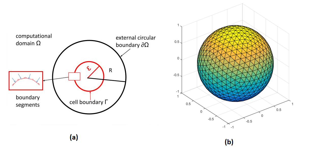
We consider the balance of momentum equation describing the forces that are exerted by a closed surface (for instance by the surface of a biological cell) or curve on its direct environment; see Fig. 1, which shows a schematic of the geometry of the computational domain ($\Omega$) and the cell. Here, the cell is strictly embedded in the computational domain and the region in the cell (contained within the cell boundary) is also part of the computational domain $\Omega$, where $\Omega$ is open, simply connected with a Lipschitz boundary.

Refer to caption
Figure 1: a) Geometry and distribution of mesh points in $\mathbb{R}^{2}$. The circular cell boundary (red-circular marker) with radius $\epsilon$ is divided into finite number of line-segments (mesh points), at the mid-point of each of which point forces are applied (shown with blue-arrows). The outer circular boundary (black circular marker) with radius R over which we evaluate the two-dimensional Green’s function. b) For three dimensions, the cell boundary is approximated by mesh points and connecting triangles. Then the three-dimensional fundamental solution for the displacement is evaluated.

Upon neglecting the inertial effects, the balance of momentum gives

$$-\nabla\cdot\bf{\sigma}=\bf f.$$ (1)

Here $\bf{\sigma}$ represents the stress tensor and $\bf{f}$ denotes the body force vector. In our application, this force is exerted from the cell boundary, which is located within the domain of computation $\Omega$. We consider a homogeneous, linear and isotropic material (i.e. both intra-cellular and extracellular environment). For small displacements, $\mathbf{\sigma}$ is described by Hooke’s Law:

$$\mathbf{\sigma}=\frac{E}{1+\nu}\left\{\epsilon+\frac{\nu}{1-2\nu}tr(\epsilon)\mathbf{I}\right\},$$ (2)

where $E$ is the Young’s Modulus of the material (cell and immediate surroundings), $\nu$ is the Poisson’s ratio and $\mathbf{\epsilon}$ is the infinitesimal strain tensor given by:

$$\mathbf{\epsilon=}\frac{1}{2}\left[\mathbf{\nabla u+(\nabla u)}^{T}\right].$$ (3)

Here $\bf{u}$ represents the displacement vector. In the 2D case, we split the cell boundary (denoted by $\Gamma$ in Figure 1(a)) into $m$ line segments by $m$ mesh points. On the midpoint of each line segment, we position the point of action of a point force, expressed by Dirac delta distributions. The Dirac measure is defined by

$\displaystyle\delta({\bf x})=0,\qquad{\bf x}\neq{\bf 0},$

and for any open portion $D\subset\mathbb{R}^{d}$ that contains ${\bf 0}$, we have

$\displaystyle\int_{D}\delta({\bf x})d{\bf x}=1.$

Having $m$ midpoints, the total force exerted by the cell is given by [25]:

$$\mathbf{f=}\sum\limits_{j=1}^{m}Q(\mathbf{x})\mathbf{n}(\mathbf{x}_{j})\delta(\mathbf{x}-\mathbf{x}_{j})\Delta\Gamma(\mathbf{x}_{j}),$$ (4)

For a continuous treatment of the cell boundary, we end up with an integral form of the total force,

$$\mathbf{f}=\int_{\Gamma}Q(\boldsymbol{x}^{\prime})\boldsymbol{n}(\boldsymbol{x}^{\prime})\delta(\boldsymbol{x}-\boldsymbol{x}^{\prime})d\Gamma(\boldsymbol{x}^{\prime}),$$ (5)

where $Q(\mathbf{x})$ is the magnitude of the pulling or pushing force exerted at point $\mathbf{x}$ per unit length, $\mathbf{n}(\mathbf{x}_{j})$ is the unit inward pointing normal vector (towards the centre of the cell) at position $\mathbf{x}$, $\mathbf{x}_{j}$ is the midpoint on line segment $j$ of the cell and $\Delta\Gamma(\mathbf{x}_{j})$ is the length of line segment $j$. For the sake of simplicity, any time dependencies and the physical units of the parameters are neglected. Furthermore, different types of boundary conditions for the computational domain can be considered. In this study, we use homogeneous Dirichlet boundary conditions, which reflect no displacement. One could alternatively consider mixed boundary conditions, which model the material beyond the surroundings of the cell as an elastic medium by means of spring forces.

We remark that in the 3D case, we consider a surface, in which the surface is divided into meshpoints that are connected via triangles (see Figure 1(b)). On the centre point of each triangle, we assign a point source. The 3D Green’s function is evaluated on the boundary of a spherical cell with the consideration of a point, line segment and plane segment lying outside the cell. (see Figure 3(a)-(b)). Subsequently, like in the 2D case, summation over all triangles is performed, which is compared to an integral over the surface. Eqs (4) and (5) remain the same, except that they involve an area (triangular element) instead of a length (line element). The numerical experiments are conducted to validate the theoretical findings for a circle and sphere in 2D and 3D, respectively.

2.2  Fundamental Solutions to Linear Elasticity Equations

Green’s functions are often called fundamental solutions to (partial) differential equations (PDEs). In a linear (partial) differential equation with generic linear differential operator $L$, fundamental solutions mostly obey

$$Lu=\delta({\bf x}-{\bf x}^{\prime}),\qquad\text{ in }\Omega,$$

where ${\bf x}^{\prime}\in\Omega$. Alternatives are known with Dirac measures acting in the boundary conditions. In time-dependent PDEs, the Dirac measure can also act in the initial condition. Using the superposition principle, one constructs integral expressions that involve a convolution of the right-hand side with the fundamental solution as formal solutions. Existence of the integral may be used as a way to demonstrate existence of a solution possessing a certain degree of regularity in some cases. Generally speaking, closed form expressions for fundamental solutions are only available for linear PDEs with homogeneous, isotropic, constant parameters. It is widely-known that the solution of

$$-\Delta u=-\nabla\cdot(\nabla u)=\delta(\mathbf{x}),$$

is given by

$$u(\boldsymbol{x})=\begin{cases}\frac{1}{2}(x+1)-(x)_{+},&\text{in }(-1,1)\subset\mathbb{R},\text{(or in any subdomain of}~{}\mathbb{R})\\[6.45831pt] -\frac{1}{2\pi}\ln||\boldsymbol{x}||,&\text{in }\mathbb{R}^{2},\\[6.45831pt] \frac{1}{4\pi||\boldsymbol{x}||},&\text{in }\mathbb{R}^{3},\end{cases}$$

where $(x)_{+}=\max\{0,x\}$. In 1D, the fundamental solution is continuous, but possesses an isolated discontinuity of the derivative at $x=0$, which does not prevent the solution from being in $H^{1}$. However, for higher dimensionality, the solution possesses a singularity at ${\bf x}={\bf 0}$, which makes the solution in $L^{2}$ but not in $H^{1}$. Hence the solution does not lie within the space spanned by $H^{1}$ Lagrangian elements, which are often used in classical finite element methods (FEM). On the other hand for $\Omega\subset\mathbb{R}^{d}$

$$C^{\infty}_{0}(\Omega)\subset H^{1}_{0}(\Omega)\subset L^{2}(\Omega),$$

and since $C^{\infty}_{0}(\Omega)$ is dense in $L^{2}(\Omega)$, it follows that $H^{1}_{0}(\Omega)$ is dense in $L^{2}(\Omega)$. Further for the fundamental solution, we have $u\in L^{2}(\Omega)$, therefore the solution can be approximated arbitrarily well by spans of functions in $H^{1}_{0}(\Omega)$, provided that we take a sufficient number of these functions. The convergence rate, however, is jeopardized by the solution not being in $H^{1}_{0}(\Omega)$. For this reason, one seeks the solution in weighted finite element (Sobolev) spaces [6] or in different Sobolev norms, such as $W^{1,1}$ [13], or one assesses the convergence of the finite element solution away from the point of action of the Dirac delta distribution [20].

Boon & Vermolen [6] assessed well-posedness in weighted Sobolev spaces in $\mathbb{R}^{2}$ for the elasticity equation with a Dirac point force. The problem is given by

$$-\nabla\cdot\sigma={\mathbf{F}}~{}\delta({\boldsymbol{x}}-{\boldsymbol{x}}^{\prime}),$$ (6)

with fundamental solution for the displacement vector

$$\boldsymbol{u}(\boldsymbol{x})=\boldsymbol{G}(\boldsymbol{x},\boldsymbol{x}^{\prime})\boldsymbol{F},$$ (7)

where the Green’s tensor given by [23]

$$\boldsymbol{G}(\boldsymbol{x},\boldsymbol{x}^{\prime})=\left\{\begin{array}[]{ll}\displaystyle{\ -\frac{1}{8\pi\mu(1-\nu)}\left((3-4\nu)\log(||{\boldsymbol{x}}-{\boldsymbol{x}}^{\prime}||){\boldsymbol{I_{2}}}+\frac{({\boldsymbol{x}}-{\boldsymbol{x}}^{\prime})\otimes({\boldsymbol{x}}-{\boldsymbol{x}}^{\prime})}{||{\boldsymbol{x}}-{\boldsymbol{x}}^{\prime}||^{2}}\right)},&\text{in }\mathbb{R}^{2}\\ &\\ \displaystyle{\frac{1+\nu}{16\pi E(1-\nu)}\left[\frac{(3-4\nu)\boldsymbol{I}_{3}}{||\boldsymbol{x}-\boldsymbol{x}^{\prime}||}+\frac{(\boldsymbol{x}-\boldsymbol{x}^{\prime})\otimes(\boldsymbol{x}-\boldsymbol{x}^{\prime})}{||\boldsymbol{x}-\boldsymbol{x}^{\prime}||^{3}}\right]},&\text{in }\mathbb{R}^{3}\end{array}\right.$$ (8)

The Lamé coefficients $\mu$ and $\lambda$ are related to the Young’s Modulus and Poisson ratio through the following equations:

$$\mu=\frac{E}{2(1+\nu)}\text{ and }\lambda=\frac{E\nu}{(1+\nu)(1-2\nu)}.$$ (9)

We note that the elasticity differential operator (in fact the entire system) is linear, which allows the use of the superposition principle [27]. Having a linear combination of point sources over the cell boundary, gives

$$-\nabla\cdot\boldsymbol{\sigma}(\boldsymbol{u}_{1}^{\ast})=\sum\limits_{j=1}^{m}Q(\boldsymbol{x}_{j})\boldsymbol{n}(\boldsymbol{x}_{j})\delta(\boldsymbol{x}-\boldsymbol{x}_{j})\Delta\Gamma(\boldsymbol{x}_{j}),$$ (10)

with analytical solution

$${\boldsymbol{u}}_{1}^{\ast}({\boldsymbol{x}})=\sum\limits_{j=1}^{m}Q(\boldsymbol{x}_{j})\boldsymbol{G}(\boldsymbol{x},\boldsymbol{x}_{j})\boldsymbol{n}(\boldsymbol{x}_{j})\Delta\Gamma(\boldsymbol{x}_{j}).$$ (11)

For a continuous treatment of the cell boundary, we end up with an integral term in the right-hand side (RHS) of the PDE, given by

$$-\nabla\cdot\boldsymbol{\sigma}(\boldsymbol{u}_{2}^{\ast})=\int_{\Gamma}Q(\boldsymbol{x}^{\prime})\boldsymbol{n}(\boldsymbol{x}^{\prime})\delta(\boldsymbol{x}-\boldsymbol{x}^{\prime})d\Gamma(\boldsymbol{x}^{\prime}),$$ (12)

with analytical solution

$$\boldsymbol{u}_{2}^{\ast}(\boldsymbol{x})=\int_{\Gamma}Q(\boldsymbol{x}^{\prime})\boldsymbol{G}(\boldsymbol{x},\boldsymbol{x}^{\prime})\boldsymbol{n}(\boldsymbol{x}^{\prime})d\Gamma(\boldsymbol{x}^{\prime}).$$ (13)

Eqs (10)–(13) hold for $\mathbb{R}^{2}$ and $\mathbb{R}^{3}$, respectively. We will analyze the convergence of $\boldsymbol{u}_{1}^{\ast}(\boldsymbol{x})$ and $\boldsymbol{u}_{2}^{\ast}(\boldsymbol{x})$ in $\mathbb{R}^{d}$ and subsequently the convergence of the solution on a compact subset $\bar{\Omega}$. In Peng and Vermolen [25], convergence of the finite element solution with linear Lagrangian basis functions was considered.

3  Singularity Removing Technique and Convergence Analysis

This section provides a description of our proposed technique (singularity removing technique) in the immersed boundary method and corresponding convergence analysis between two forms of cellular forces defined in Eqs (4) and (5) in $\mathbb{R}^{2}$ and $\mathbb{R}^{3}$.

3.1  Singularity Removing Technique

First we show that the solution in Eq (8) is not in $H^{1}(\Omega)$. It suffices to treat the logarithmic part only. Consider the integral of the given term over an open ball with radius $R>0$ containing the origin, that is over $B(0,R)$, we have

$$\int_{B(0,R)}\|\nabla\log(\|{\boldsymbol{x}}\|)\|^{2}~{}d{\bf{x}}=\int_{0}^{2\pi}\int_{0}^{R}\big{(}\frac{1}{r}\big{)}^{2}~{}rd{r}d\theta=2\pi\int_{0}^{R}\frac{1}{r}~{}d{r},$$ (14)

which diverges. Hence the logarithmic part of the solution is not in $H^{1}$, and therefore the fundamental solution, see Eq (8), as a whole, in an isotropic open bounded domain is not in ${{H}}^{1}(\Omega)$. In [24], Theorem 2, it was proved that the fundamental solution of the 3D-case, see the second equation in expression (8), is not in $H^{1}(\Omega)$ either.

From now on, $\Omega$ is a non-empty, open, bounded, simply connected Lipschitz domain in $\mathbb{R}^{d}$, where either $d=2$ or $d=3$. The boundary of $\Omega$ is denoted by $\partial\Omega$, and the closure of $\Omega$ is denoted by $\bar{\Omega}=\Omega\cup\partial\Omega$. On $\Gamma\subsetneq\Omega$ forces are applied in the normal direction ${\bf n}$, where $\Gamma$ is a closed (begin and end point of the curve coincide) curve or surface, respectively, in $\mathbb{R}^{2}$ or $\mathbb{R}^{3}$. We take $\Gamma$ as closed in the interest of our applications, however, the analysis can be extended easily to cases where $\Gamma$ is not closed. The idea [16] of having a particular solution in combination with a solution to the homogeneous elasticity equation with the fundamental solution as a boundary condition (singularity removal method) can be used to demonstrate that the solution in a bounded domain in $\mathbb{R}^{d}$, $d>1$, is not in $H^{1}$ either.

Let ${\bf u}_{1}$ solve

$\displaystyle-\nabla\cdot{\bf\sigma}({\bf u_{1}})=\sum\limits_{j=1}^{m}Q(\boldsymbol{x}_{j})\boldsymbol{n}(\boldsymbol{x}_{j})\delta(\boldsymbol{x}-\boldsymbol{x}_{j})\Delta\Gamma(\boldsymbol{x}_{j}),\qquad{\bf x}\in\Omega,$

and ${\bf u}_{2}$ solve

$\displaystyle-\nabla\cdot{\bf\sigma}({\bf u_{2}})=\int_{\Gamma}Q(\boldsymbol{x}^{\prime})\boldsymbol{n}(\boldsymbol{x}^{\prime})\delta(\boldsymbol{x}-\boldsymbol{x}^{\prime})d\Gamma(\boldsymbol{x}^{\prime}),\qquad{\bf x}\in\Omega,$

with boundary condition

$\displaystyle{\bf u}_{p}|_{\partial\Omega}=0,\qquad p=1,2.$

In the singularity removing technique, we follow the procedures outlined in Gjerde et al [16], and we write the solution ${\bf u}_{p}$ by

$\displaystyle{\bf u}_{p}={\bf u}_{p}^{*}+{\bf v}_{p},$

where we introduce the expressions ${\bf u}_{p}\in\{{\bf u}_{1},{\bf u}_{2}\},{\bf u}^{*}_{p}\in\{{\bf u}^{*}_{1},{\bf u}^{*}_{2}\}\text{~{}and~{}}{\bf v}_{p}\in\{{\bf v}_{1},{\bf v}_{2}\}$ being the original solutions (in $\Omega$), closed form (based on fundamental solutions) solutions (in $\mathbb{R}^{d}$) and homogeneous solutions (in $\Omega$) to the two forms of cellular forces respectively. Note that $p=1$ and $p=2$, respectively, refer to the solutions in the summation setting and the integral setting of the boundary forces. It follows that ${\bf v}_{p}$ solves the following homogeneous boundary value problem:

$$(BVP)\left\{\begin{array}[]{cc}-\nabla\cdot\sigma({\bf v}_{p})={\bf 0},&\text{ in }\Omega,\\ {\bf v}_{p}({\bf x})=-{\bf u}_{p}^{*}({\bf x}).&\text{ in }\partial\Omega.\end{array}\right.$$ (15)

Note that ${\bf u}_{p},{\bf u}_{p}^{*}\notin{\bf{H}}^{1}(\Omega)$.
We are interested in the existence of the weak solution to the above problem, as well as in the relation between ${\bf v}_{p}$ and ${\bf u}_{p}^{*}$ in terms of $L^{2}$-norms. The existence of a unique solution to the following weak form, given by
(WF): Find ${\bf v}_{p}\in{\bf H}^{1}(\Omega)$ subject to ${\bf v}_{p}|_{\partial\Omega}=-{\bf u}_{p}^{*}$ such that, for all ${\bf\phi}\in{\bf H}_{0}^{1}(\Omega)$, we have

$\displaystyle\text{a}({\bf v}_{p},{\bf\phi)}=0,$

where

$$\text{a}(\mathbf{\mathbf{v_{p},~{}}\phi})={\int_{\Omega}\mathbf{\sigma\mathbf{(\mathbf{v}_{p})}}\mathbf{:\epsilon(\phi)}d\Omega},$$

will be proved in the next subsection. It is obvious that $\text{a}(.,.)$ is a bilinear form. In the next section, we will motivate the existence and uniqueness of the solution in ${\bf H}^{1}(\Omega)$ to this problem by setting ${\bf v}_{p}={\bf v}_{p}^{H}+{\bf v}_{p}^{P}$, where ${\bf v}_{p}^{P}|_{\partial\Omega}={\bf v}_{p}|_{\partial\Omega}=-{\bf u}_{p}^{*}({\bf x})$ and, ${\bf v}_{p}^{H}$ is the solution that satisfies the homogeneous boundary condition, under $\text{a}({\bf v}_{p}^{H},\phi)=\text{a}({\bf u}_{p}^{*},\phi)$. In order to accomplish this result, we will make use of Korn’s Inequality, boundedness of the linear forms, Lax Milgram’s Lemma and the (extended) trace theorem.

3.2  Convergence between two Forms of Cellular Forces in Immersed Boundary Method

In the current study, we investigate the linear elasticity equation (Eqns. (1)–(3)) with two forms of surface forces: the summation form (Eq. (4)) and the integral form (Eq. (5)). To verify the convergence between the solutions to both formalisms, we need to apply some classical theorems: Korn’s Inequality, Lax–Milgram’s Lemma, and the (Extended) Trace Theorem, which are stated below. We cite appropriate references for the proofs of these classical theorems.

We start with Korn’s (second) Inequality, which is indispensable for proving coerciveness of the bilinear form that corresponds to linear elasticity.

Lemma 1 (Korn’s Inequality [7]).

Let $\Omega$ be an open, bounded and connected Lipschitz domain in $\mathbb{R}^{n}$ with piecewise smooth boundary $\partial\Omega$. Then there exists a positive constant $K$, such that for any vector–valued function ${\bf u}\in{\bf H}_{0}^{1}(\Omega)$, we have

$$\int_{\Omega}||\varepsilon({\bf u})||^{2}d\Omega\geq K~{}||{\bf u}||^{2}_{{\bf H}^{1}(\Omega)}.$$

An important consequence of Korn’s Inequality is that for all ${\bf u}\in{\bf H}^{1}_{0}(\Omega)$, we have the existence of a $K>0$ such that

$\displaystyle\text{a}({\bf u},{\bf u})=\int_{\Omega}(2\mu~{}\epsilon({\bf u})+\lambda~{}tr(\epsilon({\bf u}))~{}I):\epsilon({\bf u})d\Omega=\int_{\Omega}2\mu~{}||\epsilon({\bf u})||^{2}+\lambda~{}(tr(\epsilon({\bf u})))^{2}d\Omega\geq 2\mu K||{\bf u}||^{2}_{{\bf H}^{1}(\Omega)}.$

Hence the bilinear form is coercive (strongly elliptic).

Coercivity of $\text{a}(\boldsymbol{u},\boldsymbol{u})$ implies uniqueness of ${\bf v}_{p}$ in (WF), since if there were two solutions, then their difference satisfies $a({\bf v}_{1}-{\bf v}_{2},~{}\phi)=0$, with $({\bf v}_{1}-{\bf v}_{2})|_{\partial\Omega}=0,$ for all $\phi\in{\bf H}^{1}_{0}(\Omega)$. Substituting $\phi={\bf v}_{1}-{\bf v}_{2}$ with coercivity implies $||{\bf v}_{1}-{\bf v}_{2}||_{H^{1}(\Omega)}=0$, then $\bf{v}_{1}=\bf{v}_{2}$.

An important result for the conclusion of existence and uniqueness in case of a bilinear form $\text{a}(.,.):H\times H\longrightarrow\mathbb{R}$, which follows from Riesz’ Representation Lemma for bounded, linear functions, is Lax-Milgram’s Lemma:

Lemma 2 (Lax Milgram’s Lemma [7]).

Let $H$ be a Hilbert space, let $a(\cdot,\cdot):H\times H\to\mathbb{R}$ be a continuous (bounded), coercive bilinear form, and let $f(v)$ be a bounded linear functional in $H$ (i.e., $f\in H^{-1}$). Then there exists exactly one $u\in H$ such that

$$a(u,v)=f(v),\quad\forall~{}v\in H.$$

Furthermore, $\|u\|_{H}\leq\frac{1}{c}\|f\|_{H^{-1}}$, where $a(v,v)\geq c\|v\|_{H}^{2}$, for all $v\in H$.

Lax-Milgram’s Lemma will be used to demonstrate existence of a solution to (WF). In cases where the bilinear form satisfies $\text{a}(.,.):H_{1}\times H_{2}\longrightarrow\mathbb{R}$, where $H_{1}$ and $H_{2}$ are two different Hilbert spaces such as in the case of the use of weighted Sobolev spaces, one uses Necas’ Theorem [28] as a generalization to establish existence and uniqueness. The coercivity condition is replaced with the inf-sup condition and for all $u\in H_{1}$ there must be a $v\in H_{2}$ such that $a(u,v)\neq 0$. Additionally we need the trace theorem:

Lemma 3 (Trace Theorem [1]).

Let $\Omega$ be an open, bounded and connected Lipschitz domain in $\mathbb{R}^{n}$ with piecewise smooth boundary $\partial\Omega$, then there exists a linear, continuous trace operator

$$T:H^{1}(\Omega)\to L^{2}(\partial\Omega),$$

with the continuous extension of $v$ from $\Omega$ to $\partial\Omega$

$$Tv:=v|_{\partial\Omega},\text{ for all }v\in H^{1}(\Omega)\cap C(\bar{\Omega}).$$

Continuity (Boundedness) of the trace operator implies that there exists $C_{T}>0$ such that

$$\|Tv\|_{L^{2}(\partial\Omega)}\leq C_{T}\|v\|_{H^{1}(\Omega)}\quad\text{for all }v\in H^{1}(\Omega).$$

The trace operator, $T:H^{1}(\Omega)\longrightarrow L^{2}(\partial\Omega)$, is neither surjective, nor injective. To this extent, it is surjective on $H^{1/2}(\partial\Omega)$, that is $T:H^{1}(\Omega)\longrightarrow H^{1/2}(\partial\Omega)$, where $H^{1/2}(\partial\Omega)$ is formally defined by

$\displaystyle H^{1/2}(\partial\Omega):=\{u\in L^{2}(\partial\Omega):\exists~{}w\in H^{1}(\Omega)\text{ such that }Tw=u\}.$

Since $T$ is surjective on $H^{1/2}(\partial\Omega)$, the trace operator has a right inverse operator $E:H^{1/2}(\partial\Omega)\longrightarrow H^{1}(\Omega)$ such that $T(E):H^{1/2}(\partial\Omega)\longrightarrow H^{1/2}(\partial\Omega)$, for which we formally have:

Lemma 4 (Trace Extension Theorem [1]).

Let $\Omega$ be an open, bounded and connected Lipschitz domain in $\mathbb{R}^{n}$ with smooth boundary $\partial\Omega$, then the trace operator

$$\bar{T}:H^{1}(\Omega)\to H^{1/2}(\partial\Omega)\subset L^{2}(\partial\Omega),$$

is surjective and hence has a continuous right inverse operator

$$E:H^{1/2}(\partial\Omega)\to H^{1}(\Omega),$$

satisfying

$$(\bar{T}\circ E)(w)=w\quad\text{for all }w\in H^{1/2}(\partial\Omega).$$

From continuity, there exists a constant $C_{I}>0$ such that

$$\|Ew\|_{H^{1}(\Omega)}\leq C_{I}\|w\|_{H^{1/2}(\partial\Omega)},\quad\text{for all }w\in H^{1/2}(\partial\Omega).$$

The above concepts will be used in the analysis that follows.

We establish existence of ${\bf v}_{p}\in{\bf H}^{1}(\Omega)$ in weak form (WF). From now on, we more or less follow the presentation by Lions and Magenes [22]. Since ${\bf u}_{p}^{*}$ is smooth on $\partial\Omega$, and assuming that $\partial\Omega$ is Lipschitz, it follows from the Trace Extension Theorem that there is a ${\bf v}_{p}^{P}=E({\bf u}_{p}^{*}|_{\partial\Omega})\in{\bf H}^{1}(\Omega)$ such that $T({\bf v}_{p}^{P})={\bf u}_{p}^{*}|_{\partial\Omega}$ (that is ${\bf u}_{p}^{*}|_{\partial\Omega}\in H^{1/2}(\partial\Omega)$), for which

$$||{\bf v}_{p}^{P}||_{{\bf H}^{1}(\Omega)}\leq C_{I}||u_{p}^{*}||_{L^{2}(\partial\Omega)},$$

for a $C_{I}=C_{I}(\Omega)>0$. To this extent, we write ${\bf v}_{p}={\bf v}_{p}^{H}+{\bf v}_{p}^{P}$, where ${\bf v}_{p}^{P}|_{\partial\Omega}=-{\bf u}_{p}^{*}({\bf x})$. This gives

$\displaystyle\text{Find ${\bf v}_{p}^{H}\in{\bf H}^{1}_{0}(\Omega)$ such that }\text{a}({\bf v}_{p}^{H},\phi)=\text{a}({\bf u}_{p}^{P},\phi),\text{ for all $\phi\in{\bf H}_{0}^{1}(\Omega)$.}$

By substitution and some algebraic manipulations, it follows that the bilinear form is bounded in ${\bf H}^{1}_{0}(\Omega)$. The right-hand side is then also bounded in $\phi\in{\bf H}^{1}_{0}(\Omega)$. Together with coerciveness, it follows from Lax-Milgram’s Lemma that there exists a ${\bf v}_{p}^{H}\in{\bf H}_{0}^{1}(\Omega)$ that solves the above variational problem. Since we observed that ${\bf v}_{p}^{P}$ exists in ${\bf H}^{1}(\Omega)$, it follows that ${\bf v}_{p}={\bf v}_{p}^{P}+{\bf v}_{p}^{H}$ exists in ${\bf H}^{1}(\Omega)$. We also saw earlier that there is at most one ${\bf v}_{p}\in{\bf H}^{1}(\Omega)$. Hence we proved the following lemma:

Lemma 5.

Variational problem (WF) has one and only one solution ${\bf v}_{p}\in{\bf H}^{1}(\Omega)$.

Subsequently, we treat the following boundary value problem on a bounded domain for a general dimension ($d\geq 1$).

$$(BVP_{1})\left\{\begin{array}[]{cc}-\nabla\cdot\mathbf{\sigma\mathbf{(\boldsymbol{u}_{1})}=}\sum\limits_{j=1}^{m}Q\mathbf{(\mathbf{x}}_{j}\mathbf{)\mathbf{n}(\mathbf{x}}_{j}\mathbf{)}\delta\mathbf{(\mathbf{x}-\mathbf{x}}_{j}\mathbf{)\Delta\Gamma(\mathbf{x}}_{j}\mathbf{),}&\text{in }\Omega,\\ {\bf u}_{1}={\bf 0},&\text{on }\partial\Omega.\end{array}\right.$$ (16)

Furthermore, we consider the continuous boundary value problem on a bounded domain, given by

$$(BVP_{2})\left\{\begin{array}[]{cc}{-\nabla\cdot\mathbf{\sigma\mathbf{({\boldsymbol{u}}_{2})}=}\int_{\Gamma}Q\mathbf{(\mathbf{x}}^{\prime}\mathbf{)\mathbf{n}(\mathbf{x}}^{\prime}\mathbf{)}\delta\mathbf{(\mathbf{x}-\mathbf{x}}^{\prime}\mathbf{)}d\Gamma\mathbf{(x}^{\prime}\mathbf{),}}&\text{in }\Omega,\\ {\bf u}_{2}={\bf 0},&\text{on }\partial\Omega.\end{array}\right.$$ (17)

Our objective is to prove the convergence between the solution of (BVP1) and the solution of (BVP2) as $m\longrightarrow\infty$. First we will estimate an upper bound of $|\boldsymbol{u}_{1}^{\ast}-{\boldsymbol{u}}_{2}^{\ast}|$, where ${\bf u}_{p}^{*}$ denote the fundamental solutions (i.e. Green’s function) in $\mathbb{R}^{d}$. Before we do so, we establish the following lemma regarding numerical integration, which amounts to a multi-dimensional generalization of the standard composite midpoint rule, over a polygon.

Lemma 6.

Let $\Gamma_{p}$ be a polygon, a closed curve consisting of line segments $\tilde{\Gamma}_{q}$, embedded in $\Omega\subset\mathbb{R}^{2}$ that is composed of a union of line segments $\Delta\Gamma_{j}$, that is ${\Gamma_{p}=\bigcup_{j=1}^{m}\Delta\Gamma_{j}}$, such that each $\tilde{\Gamma}_{q}$ consists of an integer number of line segments $\Delta\Gamma_{p}$. Further, let line segment $\Delta\Gamma_{j}$ be bounded by vertices ${\bf x}_{j}$ and ${\bf x}_{j+1}$, such that ${\bf x}_{m+1}={\bf x}_{1}$, and let ${\bf x}_{j+\frac{1}{2}}$ be the midpoint of a line segment $\Delta\Gamma_{j}$, and let $f$ be a $C^{2}$–smooth function that is defined over an open set that includes $\Gamma_{p}$. Then there exists a $C_{1}>0$, such that

$$\bigg{|}\int_{\Gamma_{p}}fd\Gamma-\sum_{j=1}^{m}f({\bf x}_{j+\frac{1}{2}})||{\bf x}_{j+1}-{\bf x}_{j}||\bigg{|}\leq C_{1}h^{2}.$$

where $h=\text{max}_{j\in{\{1,...,m}\}}\parallel\mathbf{x}_{j+1}-\mathbf{x}_{j}\parallel$.

In three dimensions, let $\Gamma_{p}$ be a closed surface in $\Omega\subset\mathbb{R}^{3}$, that is composed of a union of surface segments $\Delta\tilde{\Gamma}_{q}$. Let $\Gamma_{p}$ be divided by triangular elements $\Delta\Gamma_{j}$, such that ${\Gamma_{p}=\bigcup_{j=1}^{m}\Delta\Gamma_{j}}$, let ${\bf x}_{j}$ be the centre of $\Delta\Gamma_{j}$, then there exists a positive constant $C_{2}$, such that for each component we have

$$\left|\int_{\Gamma_{p}}f(\bf{x})\,d{\bf{x}}-\sum_{j=1}^{m}\frac{|\Delta_{j}|}{2}f({\bf{x}}_{j})\right|\leq{C_{2}}h{{}^{2}},$$

where $h$ is the maximal diameter among all the surface elements over $\Gamma_{p}$ and $|\Delta_{j}|/2$ is the area of the (triangular) surface element $\Delta\Gamma_{j}$.

Proof.

First we treat the 2D case of a closed curve. Using a midpoint rule for a multivariate function, let us consider

$$\mathbf{x}(s)=\mathbf{x}_{j+\frac{1}{2}}+\frac{s}{2}{(\mathbf{x}_{j+1}-\mathbf{x}_{j})},\quad-1\leq s\leq 1,$$

Hence, $\mathbf{x}(0)=\mathbf{x}_{j+1/2}\quad\text{and}\quad{\mathbf{x}^{{}^{\prime}}(s)}=\frac{1}{2}(\mathbf{x}_{j+1}-\mathbf{x}_{j})$, and therefore,

$$\parallel{\mathbf{x}^{{}^{\prime}}(s)}\parallel=\frac{1}{2}\parallel(\mathbf{x}_{j+1}-\mathbf{x}_{j})\parallel.$$

We calculate the contribution over a line segment $\Delta\Gamma_{j}$:

$$\int\limits_{\Delta\Gamma_{j}}f({\bf x})d\Gamma=\int_{-1}^{1}f({\bf x}(s))\parallel\mathbf{x^{{}^{\prime}}(s)}\parallel ds=\frac{1}{2}\parallel\mathbf{x}_{j+1}-\mathbf{x}_{j}\parallel\int_{-1}^{1}f(\mathbf{x}(s))ds.$$

Let $\mathbf{H(x}(s))$ be the Hessian matrix of $f\mathbf{(x}(s))$, then Taylor’s Theorem warrants the existence of a $\hat{s}\in(-1,1)$ such that

$\displaystyle\int\limits_{\Delta\Gamma_{j}}f({\bf x})d\Gamma$ $\displaystyle=\frac{1}{2}\parallel\mathbf{x}_{j+1}-\mathbf{x}_{j}\parallel\int_{-1}^{1}f({\bf x}(0))+\frac{s}{2}({\bf x}_{j+1}-{\bf x}_{j})\nabla f(\mathbf{x}(0))$
$\displaystyle\quad+\frac{1}{2}s^{2}\left(\frac{\mathbf{x}_{j+1}-\mathbf{x}_{j}}{2}\right)^{T}\mathbf{H(x}(\hat{s}))(\frac{\mathbf{x}_{j+1}-\mathbf{x}_{j}}{2})ds$
$\displaystyle=\frac{1}{2}\parallel\mathbf{x}_{j+1}-\mathbf{x}_{j}\parallel\left[2~{}f({\bf x}_{j+1/2})+0+\frac{1}{12}(\mathbf{x}_{j+1}-\mathbf{x}_{j})^{T}\mathbf{H(x}(\hat{s}))(\mathbf{x}_{j+1}-\mathbf{x}_{j})\right]$
$\displaystyle=\parallel\mathbf{x}_{j+1}-\mathbf{x}_{j}\parallel f({\bf x}_{j+1/2})+\frac{1}{24}\parallel\mathbf{x}_{j+1}-\mathbf{x}_{j}\parallel(\mathbf{x}_{j+1}-\mathbf{x}_{j})^{T}\mathbf{H(x}(\hat{s}))(\mathbf{x}_{j+1}-\mathbf{x}_{j}),$

Since $f$ is smooth in an open region around $\Gamma_{p}$, it follows that there exists a $\hat{K}_{j}>0$ (maximum eigenvalue), such that

$$\big{|}\mathbf{(x,H(x))}\big{|}\leq\hat{K}_{j}\parallel\mathbf{x}\parallel^{2},\\ \text{on }\Delta\Gamma_{j}.$$

Therefore, we obtain that

$\displaystyle\bigg{|}\int\limits_{\Delta\Gamma_{j}}f({\bf x})d\Gamma-\parallel\mathbf{x}_{j+1}-\mathbf{x}_{j}\parallel f({\bf x}_{j+1/2})\bigg{|}\leq\frac{1}{24}\hat{K}_{j}\parallel\mathbf{x}_{j+1}-\mathbf{x}_{j}\parallel^{3}.$

Let $\hat{K}=\max_{j}(\hat{K}_{j})$, then summation of the boundary elements over ${\Gamma}_{p}$ gives

$\displaystyle\begin{split}\bigg{|}\int\limits_{\Gamma_{p}}{f({\bf x})}d\Gamma-\sum_{j=1}^{m}\parallel\mathbf{x}_{j+1}-\mathbf{x}_{j}\parallel f({\bf x}_{j+\frac{1}{2}})\bigg{|}\leq\sum_{j=1}^{m}\bigg{|}\int\limits_{\Delta\Gamma_{j}}{f({\bf x})}d\Gamma-\parallel\mathbf{x}_{j+1}-\mathbf{x}_{j}\parallel f({\bf x}_{j+\frac{1}{2}})\bigg{|}\leq\\ \frac{1}{24}\hat{K}\sum_{j=1}^{m}\parallel\mathbf{x}_{j+1}-\mathbf{x}_{j}\parallel^{3}\leq\frac{1}{24}\hat{K}\ \text{max}_{j\in{\{1,...,m}\}}(\parallel\mathbf{x}_{j+1}-\mathbf{x}_{j}\parallel^{2})\cdot\big{|}\Gamma_{p}\big{|}=\frac{1}{24}\hat{K}h^{2}\big{|}\Gamma_{p}\big{|},\end{split}$

where $h=\text{max}_{j\in{\{1,...,m}\}}\parallel\mathbf{x}_{j+1}-\mathbf{x}_{j}\parallel$, and $|{\Gamma}_{p}|$ is the perimeter of the polygon ${\Gamma}_{p}$.
Subsequently, we treat the three dimensional case. In three dimensions, the surface element over a manifold is a patch of a surface (a portion of a plane, i.e a triangle). Suppose $e_{j}$ is a triangular surface element in three dimensional space with vertices $({\bf{x}}_{1},{\bf{x}}_{2},{\bf{x}}_{3})$. We compute the midpoint ${\bf{x}}_{c}$ of $e_{j}$ as ${\bf{x}}_{c}=\frac{1}{3}({\bf{x}}_{1}+{\bf{x}}_{2}+{\bf{x}}_{3})$. We map the triangle in $(x,y,z)-$space to the reference triangle in $(s,t)$-space with points $(s_{1},t_{1})=(0,0),~{}(s_{2},t_{2})=(1,0)$ and $(s_{3},t_{3})=(0,1)$. The parameterization from the reference triangle $e_{0}$ to the original (physical) triangle $e_{j}$ is given by

$${\bf{x}}(s,t)={\bf{x}}_{1}(1-s-t)+s{\bf{x}}_{2}+t{\bf{x}}_{3},\quad 0\leq s\leq 1,\quad 0\leq t\leq 1-s.$$

For any function $f({\bf{x}})\in C^{2}(\Omega)$, the integral of $f(\bf{x})$ over the original triangle is given by

$${\int_{e_{j}}}f({\bf{x}})d{{\bf{x}}}={\int_{e_{0}}}f({\bf{x}}(s,t))|\Delta_{j}|d(s,t),$$

where $|\Delta_{j}|=\sqrt{|\det({\bf{J}}^{T}{\bf{J}})|}$, $\bf{J}$ is the Jacobian matrix, and $e_{0}=\{(s,t)\in\mathbb{R}^{2}:0\leq s\leq 1,0\leq t\leq 1-s\}$ given by

$${\bf{J}}=\frac{\partial(x,y,z)}{\partial(s,t)}=\begin{pmatrix}x_{2}-x_{1}&x_{3}-x_{1}\\ y_{2}-y_{1}&y_{3}-y_{1}\\ z_{2}-z_{1}&z_{3}-z_{1}\end{pmatrix},$$

and $\sqrt{|\det({\bf{J}}^{T}{\bf{J}})|}$ is twice the area of the original triangle $e_{j}$, i.e.,

$$|\Delta_{j}|:=\sqrt{|\det({\bf{J}}^{T}{\bf{J}})|}=\|({\bf{x}}_{2}-{\bf{x}}_{1})\times({\bf{x}}_{3}-{\bf{x}}_{1})\|.$$

We follow the same steps as for the two-dimensional case, where ${\bf{x}}(1/3,1/3)$ coincides with the midpoint ${\bf{x}}_{c}$ of element $e_{j}$, and where the midpoint rule (Taylor’s Theorem) for a multivariate function is used, which results into

$\displaystyle\int_{e_{j}}f({\bf x})d{{\bf x}}=\int_{e_{0}}f({\bf x}(s,t))|\Delta_{j}|d(s,t)=|\Delta_{j}|\int_{e_{0}}f({\bf x}(s,t))d(s,t)=$
$\displaystyle|\Delta_{j}|\int_{e_{0}}\left(f({\bf{x}}_{c})+({\bf{x}}(s,t)-{\bf{x}}_{c})\cdot\nabla{f}({\bf{x}}_{c})+\frac{1}{2}({\bf{x}}(s,t)-{\bf{x}}_{c})^{T}H({\bf{x}}({\hat{s}},\hat{t}))({\bf{x}}(s,t)-x_{c})\right)d(s,t)=$
$\displaystyle|\Delta_{j}|\left[\frac{1}{2}f({\bf{x}}_{c})+0+\frac{1}{2}\int_{e_{0}}({\bf{x}}(s,t)-{\bf{x}}_{c})^{T}H({\bf{x}}(\hat{s},\hat{t}))({\bf{x}}(s,t)-{\bf{x}}_{c})\,d(s,t)\right].$

Since $f({\bf x})\in C^{2}(\Omega)$, it follows that there exists a $\hat{K}_{j}>0$ (maximum eigenvalue, different from the 2D-case), such that

$$\big{|}\mathbf{(x,H(x))}\big{|}\leq\hat{K}_{j}\parallel\mathbf{x}\parallel^{2},\text{on }e_{j}.$$

Therefore, we obtain that

$$\left|\int_{e_{j}}f{\bf{(x)}}\,d{\bf{x}}-\frac{|\Delta_{j}|}{2}f{\bf{(x}}_{c})\right|\leq\left|\frac{|\Delta_{j}|}{2}\int_{e_{0}}({\bf{x}}(s,t)-{\bf{x}}_{c})^{T}{\bf{H(x}}(\hat{s},\hat{t}))({\bf{x}}(s,t)-{\bf{x}}_{c})\,d(s,t)\right|\leq\frac{|\Delta_{j}|}{4}\hat{K}_{j}{h^{2}},$$

where $h$ is the maximal diameter in the original triangle $e_{j}$.
Considering all the surface elements over $\Gamma_{p}$, we get

$$\left|\int_{\Gamma_{p}}f{\bf{(x}})\,d{\bf{x}}-\sum_{j=1}^{m}\frac{|\Delta_{j}|}{2}f{\bf{(x}}_{j})\right|\leq\frac{\hat{K}_{j}{h^{2}}}{4}\sum_{j=1}^{m}\frac{|\Delta_{j}|}{2}=\frac{\hat{K}_{j}{h^{2}}}{4}|\Gamma_{p}|,$$

where $h$ is the maximal diameter among all the surface elements (i.e., triangles) and $|\Gamma_{p}|$ is the sum of the areas (area in $\mathbb{R}^{3}$) of all the surface elements over $\Gamma_{p}$. Therefore, in three dimensions, we can conclude that there exists a constant $C_{2}>0$ such that:

$$\left|\int_{\Gamma_{p}}f{\bf{(x}})\,d{\bf{x}}-\sum_{j=1}^{m}\frac{|\Delta_{j}|}{2}f{\bf{(x}}_{j})\right|\leq{C_{2}}{h^{2}}.$$

In principle, we demonstrated the convergence of the mid-point rule for quadrature in a more generic setting. We note that this result for a generic curve or manifold was demonstrated in other works as well [25], among others, although it was not labeled as a formal result. This lemma has the following important consequence:

Corollary 1.

Let $\boldsymbol{u}_{1}^{\ast}$ and $\boldsymbol{u}_{2}^{\ast}$ be given by Eqns (11) and (13), respectively, then for all ${\bf x}\in\Omega_{\delta}=\{{\bf x}\in\Omega\ {|}\ {\rm dist}({\bf x},\Gamma)>\delta\}$, $\delta>0$ (that is away from $\Gamma$), there is a $C_{2}>0$ such that for ${\bf x}\in\Omega_{\delta}$, $|{\bf u}_{1}^{*}-{\bf u}_{2}^{*}|\leq C_{2}h^{2}$, and $\parallel\mathbf{u}_{1}^{*}-\mathbf{u}_{2}^{*}\parallel_{L^{2}(\Omega_{\delta})}\leq{C}h^{2}$. Note that here $\delta$ is a positive constant but not Dirac delta distribution.

Proof.

Since ${\bf G}({\bf x};{\bf x}^{\prime})$ is smooth for any ${\bf x}\in\Omega_{\delta}$ (away from $\Gamma$), and hence the requirements of Lemma 6 are fulfilled, we have $|{\bf u}_{1}^{*}-{\bf u}_{2}^{*}|\leq C_{2}h^{2}$ for any ${\bf x}\in\Omega_{\delta}$. Integration over $\Omega_{\delta}$ gives

$$\begin{split}\left[\int_{\Omega_{\delta}}|\mathbf{u}_{1}^{*}-\mathbf{u}_{2}^{*}|^{2}d{\Omega}\right]^{1/2}\leq\big{[}\int_{\Omega_{\delta}}C_{2}^{2}({\bf{x}})h^{4}d{\Omega}\big{]}^{1/2}\leq\sup_{{\bf x}\in\Omega_{\delta}}C_{2}({\bf{x}})h^{2}|{\Omega_{\delta}}|^{1/2}=\bar{C}h^{2}\end{split}$$

Hence,

$$\parallel\mathbf{u}_{1}^{*}-\mathbf{u}_{2}^{*}\parallel_{{L}^{2}(\Omega_{\delta})}\leq\bar{C}h^{2}.$$ (18)

Corollary 2.

Let $\bf{u}_{1}^{\ast}$ and $\bf{u}_{2}^{\ast}$ be given by Eqns (11) and (13), respectively, also let $S$ and $\tilde{\Gamma}$ be a bounded surface and curve in $\mathbb{R}^{3}$, then there are $C_{S}>0$ and $C_{\tilde{\Gamma}}>0$, such that $\parallel\mathbf{u}_{1}^{*}-\mathbf{u}_{2}^{*}\parallel_{L^{2}(S)}\leq{C_{S}}h^{2}$ and $\parallel\mathbf{u}_{1}^{*}-\mathbf{u}_{2}^{*}\parallel_{L^{2}(\tilde{\Gamma})}\leq{C_{\Gamma}}h^{2}$, respectively.

Proof.

Since ${\bf G}({\bf x};{\bf x}^{\prime})$ is smooth for any ${\bf x}\in S$, and hence the requirements of Lemma 6 are fulfilled, we have $|{\bf u}_{1}^{*}-{\bf u}_{2}^{*}|\leq C_{2}h^{2}$ for any ${\bf x}\in S$. Integration over $S$ gives

$$\begin{split}\big{[}\int_{S}|\mathbf{u}_{1}^{*}-\mathbf{u}_{2}^{*}|^{2}d{S}\big{]}^{1/2}\leq\big{[}\int_{S}C_{2}^{2}({\bf{x}})h^{4}d{S}\big{]}^{1/2}\leq\sup_{{\bf x}\in S}C_{2}({\bf{x}})h^{2}|{S}|^{1/2}=C_{S}h^{2}\end{split}$$

Hence,

$$\parallel\mathbf{u}_{1}^{*}-\mathbf{u}_{2}^{*}\parallel_{{L}^{2}(S)}\leq{C_{S}}h^{2}.$$ (19)

and analogously,

$$\parallel\mathbf{u}_{1}^{*}-\mathbf{u}_{2}^{*}\parallel_{{L}^{2}(\tilde{\Gamma})}\leq{C_{\tilde{\Gamma}}}h^{2}.$$ (20)

This claim brings us to the following important result:

Theorem 1.

Let ${\bf v}_{p}$ solve the homogeneous problem (15), subject to ${\bf v}_{p}=-{\bf u}_{p}^{*}$ on $\partial\Omega$, then there is a $K>0$ such that $||{\bf v}_{1}-{\bf v}_{2}||_{L^{2}(\Omega_{\delta}))}\leq Kh^{2}$.

Proof.

From Lemma 1, we have existence of ${\bf v}_{1},~{}{\bf v}_{2}\in{\bf H}^{1}(\Omega)$, as well as of its difference. From Corollary 1, we have,

$\displaystyle||{\bf u}_{1}^{*}-{\bf u}_{2}^{*}||^{2}_{L^{2}(\partial\Omega)}\leq Ch^{2}.$ (21)

Note that the right-hand side is a constant, hence in $H^{1/2}(\partial\Omega)\subset L^{2}(\partial\Omega)$, therefore since

$\displaystyle||{\bf v}_{1}-{\bf v}_{2}||_{L^{2}(\partial\Omega)}=||{\bf u}_{1}^{*}-{\bf u}_{2}^{*}||_{L^{2}(\partial\Omega)}\leq C_{3}h^{2},$ (22)

the Trace Extension Theorem [1] (Lemma 4 maps functions from their traces $H^{1/2}(\partial\Omega)$ to $H^{1}(\Omega)$) asserts the existence of a $\beta>0$ such that

$\displaystyle||{\bf v}_{1}-{\bf v}_{2}||_{H^{1}(\Omega)}\leq\beta||{\bf v}_{1}-{\bf v}_{2}||_{L^{2}(\partial\Omega)}=\beta||{\bf u}_{1}^{*}-{\bf u}_{2}^{*}||_{L^{2}(\partial\Omega)}\leq\beta C_{3}h^{2}.$ (23)

Since

$\displaystyle||{\bf v}_{1}-{\bf v}_{2}||_{L^{2}(\Omega)}\leq||{\bf v}_{1}-{\bf v}_{2}||_{H^{1}(\Omega)}\leq C_{4}h^{2},$ (24)

it follows that there is a $K>0$ such that

$\displaystyle||{\bf v}_{1}-{\bf v}_{2}||_{L^{2}(\Omega_{\delta})}\leq||{\bf v}_{1}-{\bf v}_{2}||_{L^{2}(\Omega)}\leq Kh^{2},$ (25)

This proves the assertion. ∎

This result brings us to the main result of the paper, namely:

Theorem 2.

Let $\bf{u_{1}}$ and $\bf{u_{2}}$ be the solutions to $(BVP_{1})$ and $(BVP_{2})$ defined in Eqs (16) and (17) respectively, then for all ${\bf x}\in\Omega_{\delta}=\{{\bf x}\in\Omega\ {|}\ dist({\bf x},\Gamma)>\delta\}$, $\delta>0$ (that is away from $\Gamma$), there is a $C_{0}>0$ such that $\parallel{\bf u}_{1}-{\bf u}_{2}\parallel_{L^{2}(\Omega_{\delta})}\leq C_{0}h^{2}$.

Proof.

Since $L^{2}(\Omega_{\delta})$ is a proper norm, we apply the triangular inequality and combining the results from Corollary 1 and relation (25), we obtain

$\displaystyle\parallel{\boldsymbol{u}}_{1}-{\boldsymbol{u}}_{2}\parallel_{L^{2}(\Omega_{\delta})}$ $\displaystyle=\parallel\mathbf{u}_{1}^{*}-\mathbf{u}_{2}^{*}+\mathbf{v}_{1}-\mathbf{v}_{2}\parallel_{L^{2}(\Omega_{\delta})}$
$\displaystyle\leq\parallel\mathbf{u}_{1}^{*}-\mathbf{u}_{2}^{*}\parallel_{L^{2}(\Omega_{\delta})}+\parallel\mathbf{v}_{1}-\mathbf{v}_{2}\parallel_{L^{2}(\Omega_{\delta})}\leq(C+K)h^{2}=C_{0}h^{2}.$

Note that the above result is valid for two- and three-dimensional cases.

4 Numerical Results

Two and three dimensional computed results are presented. The input parameters are taken from Table 1. All simulations are done by using the fundamental solutions, hence they all entail the entire fields $\mathbb{R}^{2}$ or $\mathbb{R}^{3}$. The simulations aim at demonstrating convergence of the immersed boundary method.

Table 1: Parameter values for two- and three dimensional simulation
Parameter Description Value Units Source
$E$ Young’s Modulus $1.0\times 10^{7}$ $kg/(\mu m\cdot\text{ }min^{2})$ Peng et al. [26]
$Q$ Magnitude of the force exerted on the cell $1.0\times 10^{3}$ $kg\cdot\mu m/min^{2}$ Peng et al. [26]
$R$ Radius of the boundary outside the cell $0.5$ $\mu m$ Estimated in this study
$\epsilon$ Radius of the cell $0.3$ $\mu m$ Chen et al. [9]
$\nu$ Poisson’s Ratio $0.25$ $-$ Peng et al. [26]

4.1 Two Dimensional Simulations

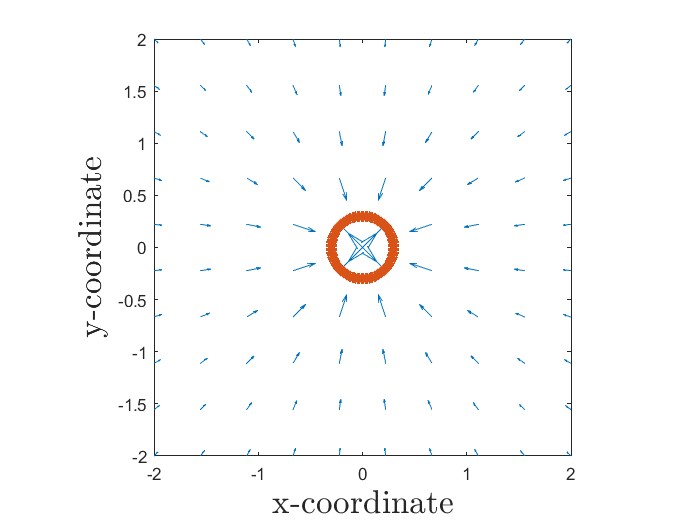
We consider a regular polygonal cell at the origin in $\mathbb{R}^{2}$ that exerts pulling or pushing forces on its direct environment. Note that as the number of line segments tends to infinity, the polygon tends to a circle. At the mid points of the line segments of the polygon, a force is applied. The magnitudes of the parameter values can be found in Table 1. For illustrational purposes, the displacement field around the cell within a box of $[-2,2]\times[-2,2]$ is shown by a vector plot in Figure 2.

Refer to caption
Figure 2: Displacement field around a circular cell, whose boundary is indicated by the red circle, in two dimensions over a grid of $10\times 10$. The displacement vectors are indicated by the blue arrows. The length of the arrows indicate the magnitude of the displacement, but does not reflect the real magnitude of the displacement. The input parameters can be found in Table 1.

We assess convergence of the solution ${\bf u}_{1}^{*}$ with respect to the number of mesh points, $m$, on the cell boundary. Convergence is quantified by the $L^{2}$–norm over the circle with midpoint at the origin and radius $R=0.5$. To approximate the $L^{2}$–norm over this circle $\partial B(0,R)$, the circle is divided into $N$ meshpoints so that a polygon results. The length of each line segment is $\Delta\Gamma$, and the midpoint of the polygon is denoted by ${\bf x}_{j}$. In this way, we obtain the following Midpoint Rule based approximation

$$||{\bf u}_{1}^{*}||_{L^{2}(\partial B(0,R)}^{2}=\int_{\partial B(0,R))}||{\bf u}_{1}^{*}||^{2}d\Gamma\approx\sum_{j=1}^{N}||{\bf u}_{1}^{*}({\bf x}_{j})||^{2}\Delta\Gamma.$$ (26)

The numerical error of this composite midpoint rule is given by $\mathcal{O}(\Delta\Gamma^{2})$. In the idealized, fully continuous case the solution of the normal component of ${\bf u}_{2}^{*}$ is fully symmetric, and hence constant over any concentric circle with the origin as midpoint. For this reason, we compute the standard deviation of the normal component of ${\bf u}_{1}^{*}$ over $\partial B(0,R)$ in Table 2. Richardson’s estimation of order of convergence [18] is used to estimate the order of convergence. It can be seen that the order of convergence of the $L^{2}$–norm is about two and that the standard deviation vanishes as $m$ increases. This result is in excellent agreement with the theory (see Corollary 2).

Table 2: Weighted $L^{2}-$norm, convergence rate and standard deviation for various values of $m$
The number of force $\text{Weighted~{}}L^{2}\text{-norm of }$ Convergence rate: Standard deviation of
points on the displacement over $q$ magnitude of
$\text{ cell boundary: }m$ $\text{circle: }\left\|\mathbf{u}_{m}\right\|_{L^{2}(\partial\Omega)}$ $\text{displacement: }STD$
10 $4.2100\times 10^{-6}$ $1.970293493$ $8.5990\times 10^{-8}$
20 $4.4263\times 10^{-6}$ $1.989583384$ $5.4848\times 10^{-10}$
40 $4.4815\times 10^{-6}$ $2.031478231$ $2.0663\times 10^{-14}$
80 $4.4954\times 10^{-6}$ $1.91753784$ $1.2235\times 10^{-20}$

4.2 Three Dimensional Simulations

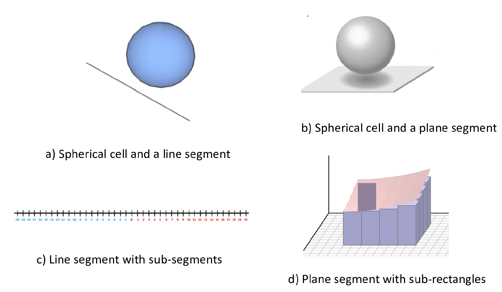
We use the same input data from Table 1 for the 3D-simulations. We consider a spherical cell with the origin as midpoint and radius $\varepsilon=0.1$. The cell surface is divided into triangles, which, in fact, gives a polyhedron, and the force is assumed to be exerted in normal direction from each point of the triangle. We assess convergence in terms of refinement, where each refinement divides each triangle into four triangles of more or less the same size. Hence each refinement more-or-less halves the diameter of the element on the cell surface. We assess convergence of the solution on a pre-selected single point, a line segment and a flat surface. Note that the point, line segment and planar surface have been chosen such that they do not intersect with the cell boundary; see Figure 3 for a schematic.

Refer to caption
Figure 3: Geometry in $\mathbb{R}^{3}$ where a spherical cell is centered at the origin i.e. $(0,0,0)$. a) A spherical cell and a line segment which is lying outside the cell (non-intersecting). b) A spherical cell and a plane which is lying outside the cell (non- intersecting). c) A line segment with sub-segments (or -divisions) on it (in context of applying the midpoint rule to the line segment). d) A plane segment divided into sub-rectangles (in context of applying the midpoint rule to the plane segment).

Over the line segment and surface, the $L^{2}$–norm is computed by a midpoint Rule. The point is positioned at $(2,0,0)$, the line (intersecting with the sphere) between $(-1,1,-1)$ and $(-1,1,1)$, the non-intersecting line between $(10,0,-1)$ and $(10,0,1)$, and the planar surface has vertices $(-1,-1,0)$ $(0,-1,0)$ $(-1,0,0)$ and $(0,0,0)$. The results are presented in Tables 3 and LABEL:Table:results_q_3D_C1. It can be seen that the order of convergence of the $L^{2}$–norm is again of order two, which is in line with the theory as in Corollary 2. For the sake of illustration, we also present some computed results in case of a line segment that intersects with the cell boundary in Tables 3 and LABEL:Table:results_q_3D_C1. It can be seen that the contact with the singularity violates the assumptions of the hypotheses of the claims that we proved, and hence the order of convergence is no longer equal to two. According to expectation, these results are therefore not in line with the theory that we developed.

Table 3: Weighted $L^{2}-$norm for various mesh refinements.
$m$ Case 1: Point Case 2(a): Line Segment Case 2(b): Line Segment Case 3: Plane Segment
(intersecting) (non-intersecting)
1 $4.464286\times 10^{-2}$ $1.008291\times 10^{-1}$ $1.263297\times 10^{-2}$ $1.687556\times 10^{-1}$
2 $4.704841\times 10^{-2}$ $1.130611\times 10^{-1}$ $1.328649\times 10^{-2}$ $1.620658\times 10^{-1}$
3 $4.766353\times 10^{-2}$ $1.174356\times 10^{-1}$ $1.345887\times 10^{-2}$ $1.602798\times 10^{-1}$
4 $4.781926\times 10^{-2}$ $1.189740\times 10^{-1}$ $1.350255\times 10^{-2}$ $1.598272\times 10^{-1}$
5 $4.785832\times 10^{-2}$ $1.195000\times 10^{-1}$ $1.346922\times 10^{-2}$ $1.597150\times 10^{-1}$
6 $4.786810\times 10^{-2}$ $1.196822\times 10^{-1}$ $1.351625\times 10^{-2}$ $1.596835\times 10^{-1}$
Table 4: Convergence rate $q$ for different mesh refinements in three dimensions. Note that the positional data is the same as in Table 3
$m$ Case 1: Point Case 2(a): Line Segment Case 2(b): Line Segment Case 3: Plane Segment
(intersecting) (non-intersecting)
1 $1.96742699696$ $1.48347027861$ $1.92263898951$ $1.90523099987$
2 $1.9818209909$ $1.5076874603$ $1.99329613008$ $1.98042359074$
3 $1.99528303923$ $1.54829596316$ $1.994725057967$ $2.01216390866$
4 $1.99778557893$ $1.52953984038$ $2$ $1.83264894222$

5 Discussion and Conclusions

We consider the immersed boundary method applied to forces that are exerted over a curve or surface within a 2D and 3D medium, respectively. The immersed boundary method is based on assigning a point force density on all the points of the curve or surface so that the overall momentum balance consists of an integral over the body force density multiplied by the Dirac delta distribution over the curve or surface. In the fields $\mathbb{R}^{d}$, $d\in\{2,3\}$, fundamental solutions for the displacement vector field are available in the case of linear elasticity. Linearity allows the superposition principle, by which the displacement vector field is constructed via a convolution of the force density field with the fundamental solution for the entire fields $\mathbb{R}^{d}$. Existence of these integrals warrants the existence of the displacement vector field as a solution to the elliptic problem (balance momentum in the entire $\mathbb{R}^{d}$–field). The solution, however, inherits the mathematical properties of the fundamental solution in the sense that the solution is not in the Hilbert space $H^{1}$, which is a classical solution space in which one searches finite element solutions. The point where the force acts defines a singularity in the fundamental solution (either one takes a logarithm in zero or divides by zero at that point). However, the solution is in $L^{2}$ in a neighbourhood containing the point where the point force acts. Furthermore, in case of a bounded computational domain, that is, the curve or surface where the point forces act is located in a finite (bounded) portion, say $\Omega\subsetneq\mathbb{R}^{d}$, one can use the so-called singularity removing (homogenization) technique where the convolution-based solution for the entire field appears as a boundary condition for the solution to the homogeneous problem in the bounded domain $\Omega$. The trace extension theorem warrants the existence and an upper boundary of a $H^{1}(\Omega)$-solution for the homogenized problem. Therewith the entire solution to the boundary value problem on a finite portion (subset) of the fields $\mathbb{R}^{d}$ is decomposed into a part in $H^{1}(\Omega)$ and another part in $L^{2}(\Omega)\setminus H^{1}(\Omega)$, which makes the overall solution reside in $L^{2}(\Omega)\setminus H^{1}(\Omega)$.

Since the integral expressions for the solution in the fields $\mathbb{R}^{d}$ amount to a computationally nasty integral to evaluate, one seeks to compute the integral numerically. This amounts to also casting the integral in the right-hand side for the forcing term in the partial differential equation into an approximating expression consisting of a summation. This can be done, for instance, by the use of the midpoint rule for integration. In the paper, we demonstrate that according to expectations of the midpoint rule, the difference in the full field solutions in $\mathbb{R}^{d}$ is of order $(\Delta\Gamma)^{2}$, where $\Delta\Gamma$ represents the diameter of a line or surface element of the portion of the domain where the forces act. The same order is recovered for the solution on a finite domain by means of the Trace Extension Theorem.

We show some numerical illustrations of the convergence of the full field solutions in $\mathbb{R}^{d}$, where the quadratic convergence behavior that was predicted by the theory is confirmed. In order to extend this to the bounded domain solutions, one has to numerically solve the equations. Although, this is a relatively straightforward task, we have omitted this in the current paper. We also note that our results are only suitable for the steady-state momentum balance equation without any damping from viscoelasticity. We are interested in extending this theory to visco-and morphoelasticity, where one also includes damping and possible growth of the medium due to microstructural changes. This lastmentioned issue is important in case of living materials and tissues.
Declaration of competing interest: The authors declare that they have no known competing financial interests or personal relationships that could have appeared to influence the work reported in this paper.
Acknowledgement: We are grateful for the financial support from the Higher Education Commission (HEC) of Pakistan in the framework of project: 1(2)/HRD/OSS-III/BATCH-3/2022/HEC/527.

References

  • Adams and Fournier [2003] R.A. Adams, J.J. Fournier, Sobolev spaces, Elsevier, 2003.
  • Bajpai et al. [2019] A. Bajpai, J. Tong, W. Qian, Y. Peng, W. Chen, The interplay between cell-cell and cell-matrix forces regulates cell migration dynamics, Biophys. J. 117 (2019) 1795–1804.
  • Barrow [1972] M.V. Barrow, Portraits of hippocrates, Med. Hist. 16 (1972) 85–88.
  • Benz [2017] E.J. Benz, Jr, The jeremiah metzger lecture cancer in the twenty-first century: An inside view from an outsider, Trans. Am. Clin. Climatol. Assoc. 128 (2017) 275–297.
  • Bertoluzza et al. [2017] S. Bertoluzza, A. Decoene, L. Lacouture, S. Martin, Local error estimates of the finite element method for an elliptic problem with a dirac source term, Numer. Methods Partial Differ. Equ. 34 (2017) 97–120.
  • Boon and Vermolen [2023] W.M. Boon, F.J. Vermolen, Analysis of linearized elasticity models with point sources in weighted sobolev spaces: applications in tissue contraction, ESAIM: Math. Model. Numer. Anal. 57 (2023) 2349–2370.
  • Braess [2001] D. Braess, Finite elements: Theory, fast solvers, and applications in solid mechanics, Cambridge University Press, 2001.
  • Byrne and Drasdo [2008] H. Byrne, D. Drasdo, Individual-based and continuum models of growing cell populations: a comparison, J. Math. Biol. 58 (2008) 657–687.
  • Chen et al. [2017] J. Chen, D. Weihs, F.J. Vermolen, A model for cell migration in non-isotropic fibrin networks with an application to pancreatic tumor islets, Biomech. Model. Mechanobiol. 17 (2017) 367–386.
  • Correia [2019] M.I.T. Correia, The Practical Handbook of Perioperative Metabolic and Nutritional Care, Academic Press, 2019.
  • Dallon et al. [1999] J.C. Dallon, J.A. Sherratt, P.K. Maini, Mathematical modelling of extracellular matrix dynamics using discrete cells: Fiber orientation and tissue regeneration, J. Theor. Biol. 199 (1999) 449–471.
  • Darby et al. [2014] I. Darby, B. Laverdet, F. Bonté, D. Alexis, Fibroblasts and myofibroblasts in wound healing, Clin. Cosmet. Investig. Dermatol. 7 (2014) 301–11.
  • D’Angelo [2012] C. D’Angelo, Finite element approximation of elliptic problems with dirac measure terms in weighted spaces: Applications to one- and three-dimensional coupled problems, SIAM J. Numer. Anal. 50 (2012) 194–215.
  • Enoch and Leaper [2007] S. Enoch, D. Leaper, Basic science of wound healing, Surg. (Oxford) 26 (2007) 31–37.
  • Evers et al. [2015] J.H. Evers, S.C. Hille, A. Muntean, Modelling with measures: Approximation of a mass-emitting object by a point source, Math. Biosci. Eng. 12 (2015) 357–373.
  • Gjerde et al. [2019] I.G. Gjerde, K. Kumar, J.M. Nordbotten, A singularity removal method for coupled 1d–3d flow models, Comput. Geosci. 24 (2019) 443–457.
  • Janiszewska et al. [2020] M. Janiszewska, M.C. Primi, T. Izard, Cell adhesion in cancer: Beyond the migration of single cells, J. Biol. Chem. 295 (2020) 2495–2505.
  • van Kan et al. [2005] J. van Kan, A. Segal, F.J. Vermolen, Numerical methods in scientific computing, VSSD, 2005.
  • Koppenol [2017] D. Koppenol, Biomedical implications from mathematical models for the simulation of dermal wound healing, Ph.D. thesis, TU Delft, 2017.
  • Köppl and Wohlmuth [2014] T. Köppl, B. Wohlmuth, Optimal a priori error estimates for an elliptic problem with dirac right-hand side, SIAM J. Numer. Anal. 52 (2014) 1753–1769.
  • Landén et al. [2016] N.X. Landén, D. Li, M. Ståhle1, Transition from inflammation to proliferation: a critical step during wound healing, Cell. Mol. Life. Sci. 73 (2016) 3861–3885.
  • Lions and Magenes [2012] J.L. Lions, E. Magenes, Non-homogeneous boundary value problems and applications: Vol. 1, volume 181, Springer Science & Business Media, 2012.
  • Peng and Hille [2023] Q. Peng, S.C. Hille, Quality of approximating a mass-emitting object by a point source in a diffusion model, Comput. Math. Appl. 151 (2023) 491–507.
  • Peng and Vermolen [2022a] Q. Peng, F. Vermolen, Numerical methods to compute stresses and displacements from cellular forces: Application to the contraction of tissue, J. Comput. Appl. Math. 404 (2022a) 113892.
  • Peng and Vermolen [2022b] Q. Peng, F. Vermolen, Point forces in elasticity equation and their alternatives in multi dimensions, Math. Comput. Simul. 199 (2022b) 182–201.
  • Peng et al. [2023] Q. Peng, F.J. Vermolen, D. Weihs, Physical confinement and cell proximity increase cell migration rates and invasiveness: A mathematical model of cancer cell invasion through flexible channels, J. Mech. Behav. Biomed. Mater. 142 (2023) 105843.
  • Richardson [1911] L. Richardson, The approximate arithmetical solution by finite differences of physical problems involving differential equations, with an application to the stresses in a masonry dam, Philos. Trans. R. Soc. A 210 (1911) 307–357.
  • Susanne C. Brenner [2008] L.R.S. Susanne C. Brenner, The Mathematical Theory of Finite Element Methods, Springer, 2008.
  • Tunç et al. [2023] B. Tunç, G.J. Rodin, T.E. Yankeelov, Implementing multiphysics models in fenics: Viscoelastic flows, poroelasticity, and tumor growth, Adv. Biomed. Eng. 5 (2023) 100074.
  • Yu et al. [2022] W. Yu, S. Sharma, E. Rao, A.C. Rowat, J.K. Gimzewski, D. Han, J. Rao, Cancer cell mechanobiology: a new frontier for cancer research, J. Natl. Cancer Cent. 2 (2022) 10–17.
  • Yue [2014] B. Yue, Biology of the extracellular matrix: An overview, J. Glaucoma 23 (2014) 20–23.