Individual solid-state nuclear spin qubits with coherence exceeding seconds
Abstract
The ability to coherently control and read out qubits with long coherence times in a scalable system is a crucial requirement for any quantum processor. Nuclear spins in the solid state have shown great promise as long-lived qubits [1, 2]. Control and readout of individual nuclear spin qubit registers has made major progress in the recent years using individual electron spin ancilla addressed either electrically [3, 4, 5] or optically [6, 7, 8, 9]. Here, we present a new platform for quantum information processing, consisting of 183W nuclear spin qubits adjacent to an Er3+ impurity in a CaWO4 crystal, interfaced via a superconducting resonator and detected using a microwave photon counter at 10mK. We study two nuclear spin qubits with of s and s, of s and s, respectively. We demonstrate single-shot quantum non-demolition readout of each nuclear spin qubit using the Er3+ spin as an ancilla. We introduce a new scheme for all-microwave single- and two-qubit gates, based on stimulated Raman driving of the coupled electron-nuclear spin system. We realize single- and two-qubit gates on a timescale of a few milliseconds, and prepare a decoherence-protected Bell state with 88% fidelity and of s. Our results are a proof-of-principle demonstrating the potential of solid-state nuclear spin qubits as a promising platform for quantum information processing. With the potential to scale to tens or hundreds of qubits, this platform has prospects for the development of scalable quantum processors with long-lived qubits.
I Introduction
Nuclear spins in the solid-state are attractive candidates for quantum computing, offering long coherence times and high density. However, the typically weak coupling of nuclear spins to their environment that enables such long coherence times makes their control and readout challenging. Nuclear spin qubits are usually addressed through their hyperfine coupling to an electron spin ancilla, which then needs to be detected. Electrical detection of electron spin donors in silicon enabled the demonstration of long-lived single-31P nuclear spin qubits in isotopically-enriched silicon [4], the operation of a two-31P quantum gate [5], and the preparation of a 123Sb -nuclear spin in a Schrödinger-cat state [10]. Electrical detection was used also for TbPc2 molecular quantum dots, enabling the manipulation and readout of a 159Tb nuclear spin qubit [11] and the implementation of Grover’s search algorithm [12]. Optical detection of individual NV center electron spins in diamond enabled the operation of a register of up to ten 13C nuclear spin qubits [8], the fault-tolerant operation of a logical qubit built out of a 13C nuclear-spin qubit register [9], and the demonstration of high-fidelity single- and two-qubit gates with a nuclear spin [13].
In this work, we present an alternative hybrid architecture to control and read out individual nuclear spin qubits via an electron spin ancilla by magnetically coupling this ancilla to a high-Q superconducting resonator. Requiring relatively straightforward fabrication techniques, this approach permits a single resonator to control numerous coherent spin defects. By detecting spin fluorescence [14] via a superconducting resonator using a superconducting circuit-based Single Microwave Photon Detector (SMPD) [15, 16], detection of individual electron spins has recently been demonstrated [17]. Leveraging this technique, we use single Er3+ spin impurities in a CaWO4 crystal to control and read-out neighbouring spin-1/2 183W nuclei via the hyperfine interaction. This method permits single-shot QND readout of individual 183W nuclear spin qubits [18]. Individual all-microwave qubit control is achieved by driving a stimulated Raman transition. Two-qubit gates are achieved by taking advantage of induced AC Zeeman shifts on the energy level structure of the electron and nuclear spin system. We use this to construct a CNOT gate and generate Bell states of the two nuclei. We further show that certain Bell states exist in a so-called decoherence free subspace and are inherently resilient to magnetic field noise, extending from s and s for the individual nuclei to s for the protected state.
II Device and Spin System
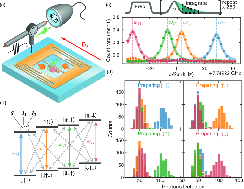
We use a crystal of CaWO4, which has tetragonal lattice symmetry, with a residual Er3+ concentration of ppb. At millikelvin temperatures, Er3+:CaWO4 behaves as an effective electron spin-1/2 system. This spin has a g-factor of 1.247 (8.38) parallel (perpendicular) to the axis of the crystal. Application of a static field lifts the two-state degeneracy via Zeeeman splitting. We pattern a planar niobium lumped-element superconducting resonator directly onto the substrate surface, as shown in Fig.1(a). The resonator has a small magnetic mode volume concentrated around a 300 nm wide, long inductor wire. This design maximises the magnetic field generated by the resonator around the wire and thus the inductive coupling to nearby electron spins. The resonator is placed inside a copper 3D cavity inside a dilution refrigerator and cooled to 11 mK. The resonator is coupled via a single antenna and circulator to an input port for drive fields and an output port to an SMPD. It is important to note that the methods described here are not unique to the nuclear or electron spin species chosen, the substrate crystal or the resonator material, and are in principle extendable to a wide range of other spin species and materials. Further details of the experimental setup are given in [18], in which the same sample and setup were used, and App.A.
We apply a magnetic field of mT along the axis of the crystal. At this field, the resonator has a frequency of GHz and a linewidth . The substrate contains many Er3+ spins with a distribution in transition frequency around a central bulk line. It is possible to probe a reduced subset of spins by tuning the magnetic field such that the and one can identify individual Er3+ spins [17]. Using this method, we choose to focus on a single Er3+ spin with interesting characteristics. The characteristic decay time of the spin was measured to be ms, dominated by spontaneous emission of photons into the resonator due to the Purcell effect [19]. We can use this to calculate the coupling of the Er3+ spin to the resonator of kHz (see App.B).
The only isotope of W with non-zero nuclear spin, 183W, has spin-1/2 and a natural abundance of 14%. The unit cell of CaWO4 contains 10 W nuclei, meaning that it is likely that one or more spins in close proximity to the Er spin will have spin-1/2. The Er spin studied in this work was chosen due to its configuration of two neighbouring spin-1/2 W nuclei. The spin Hamiltonian of this system is as follows:
| (1) |
where is the Er spin frequency, is the Erbium spin operator, are the nuclear spin frequencies, are the nuclear spin operators and , are the and hyperfine coupling constants between the electron and nuclear spins, for . Here we have kept only the hyperfine terms proportional to according to the secular approximation. This Hamiltonian gives rise to an 8 level system, as shown in Fig.1(b). In this work, we utilise the two nuclear spins as qubits, designated Qb1 and Qb2, and the electron spin as an ancilla to control and read-out the nuclear spin qubits.
Transitions between the ground and excited state of the electron spin may be directly driven via the first term in Eq.II by applying an AC magnetic field resonant with the electron spin transition via the superconducting resonator. The coupling terms give rise to four distinct electron spin transition frequencies, , , and , as indicated in Fig.1(b) by the four vertical arrows. The nuclei may in principle be driven in much the same way, however the resonator strongly suppresses fields at the requisite low drive frequencies of kHz. Therefore, we choose to prepare the nuclear spin state via cross-transitions which simultaneously flip the electron and the nuclear spin [18], as indicated by the grey arrows in Fig.1(b). These transitions are weakly allowed due to the presence of the terms in the hyperfine Hamiltonian. We pump the system into the or the nuclear spin states by driving these cross transitions using a chirped pulse which covers all necessary frequencies and allowing the electron spin to subsequently decay [18].
III Readout and Coherent Control of Single Nuclear Spins
To detect the state of the nuclear spin qubits, we repeatedly excite the electron spin at each of the 4 possible frequencies, , , and , sequentially and detect the photons emitted immediately after the excitation pulse. We sum the total number of photons counted over 200 repetitions at each frequency. The bandwidths of the resonator and SMPD, 640 kHz and kHz, respectively, are sufficient to span all 4 frequencies simultaneously. Depending on the nuclear spin state, an excess of photon counts will be detected at one of the four frequencies. Detecting this excess allows us to perform Quantum Non-Demolition (QND) readout of the joint nuclear spin state. The number of counts detected as a function of electron spin drive frequency is shown in Fig.1(c) when the system is prepared in each of the four possible nuclear spin configurations (the data here have been corrected for slow drifts in the electron spin frequency, see App.C and [18] for more details). We see that the peak photon count rate occurs at a different frequency for each of the four nuclear spin states, and that the peaks are all clearly distinguishable, allowing for high fidelity readout of the nuclear spin state. We therefore fix the drive frequencies to , , and and measure the of number of photons detected after preparing each of the 4 states for many repeated experiments to build the histograms shown in Fig.1(d). In each case, we see a clear separation between the number of photons detected after driving the transition corresponding to the prepared state vs the other three states. We threshold the number of photons detected to discriminate between the four states and measure probabilities of 0.91, 0.93, 0.92 and 0.95 to be in the desired state , , and , respectively. This is limited partially by state preparation fidelity and partially by cross-relaxation during readout via one of the sideband transitions. This leads to a small probability of a nuclear spin flip event occurring during one of the 200 excitation pulses applied to the electron at each readout frequency during readout, see App.D for further details.
Coherent control of individual nuclear spins has been achieved either by direct radio-frequency driving [11, 8], or by coupled electron-nuclear dynamics relying on the repeated application of fast, broadband, pulses to the electron spin at well-chosen time intervals [20]. In our experiment, radio-frequency driving is not possible, and the dynamical decoupling approach is not well suited for a number of reasons (high magnetic field, cavity filtering of the excitation pulses, large electron spin relaxation rate). Instead, we use stimulated Raman transitions, which are largely used in atomic physics [21]. We show that they provide a new way to achieve all-microwave single- and two-nuclear-spin-qubit gates without populating the electron spin in its excited state.
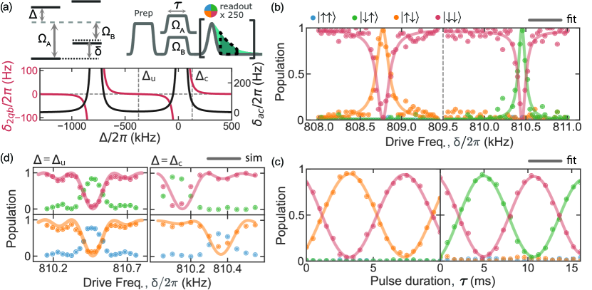
Consider first the coupling of the erbium spin to a single nuclear spin (case in Eq.1). Stimulated Raman transitions are driven by applying two simultaneous microwave tones at different frequencies and (see Fig. 2(a)), with amplitudes and . When is resonant with the frequency difference between the two ground-state levels , a transition between and can take place with an effective drive strength (see App.F). As long as , the electron spin excited levels are never significantly populated, implying that the relatively short coherence time of the electron spin transitions plays no role in the system dynamics and therefore enabling high-fidelity nuclear-spin-qubit rotations.
In addition, the Raman drives also cause ac-Zeeman frequency shifts of all the levels involved, due to the off-resonant driving of the electron transitions. As a result, the Raman resonance is found shifted by from the expected frequency (see App.F). Moreover, when the second nuclear spin is considered (), the value of is in general conditioned on the state of the other spin, giving rise to two different values, and . As such, we introduce , and . In the frame rotating at , resonant stimulated Raman driving of nuclear spin 1 is described by the effective Hamiltonian . The values of and , computed from an analytical model, are shown in Fig. 2(a). Interestingly, there is a value of , which we call (see Methods), for which . When , the Raman driving of one nuclear spin is therefore unconditional on the state of the other nuclear spin, a condition which is thus suitable for single-qubit gates. For other values of where , the Raman resonance condition of one spin is dependent on the other spin state, providing a natural way to implement two-qubit gates, as described below.
We first perform Raman spectroscopy using the unconditional driving condition kHz , and . The nuclear spin register is prepared in the state, after which a Raman pulse is applied whose detuning is swept, followed by nuclear spin readout. When the resonance condition is met, we observe a large change in the nuclear spin population to either the or the state (see Fig. 2(b)). The resonance linewidth is of order Hz or less, two orders of magnitude narrower than the electron spin linewidth, which confirms that the Raman driving occurs through virtual transitions of the electron excited states. The kHz frequency separation between the two ground-state nuclear spin transitions is due to the different values of and for each nuclear spin, due to their different position relative to the ion (see App.B). Knowing the required drive frequencies, we then prepare the state and sweep the drive duration, giving rise to coherent Rabi oscillations of each qubit, as shown in Fig.2(c). This allows us to calibrate pulses for Qb1 and Qb2, respectively.
We then study the spectrum of Qb2 after preparation of Qb1 in either the or the state (see Fig. 2(d)). If (left panel), the two resonances occur at the same frequency, confirming the unconditional driving condition. If kHz instead, the two resonances are shifted by Hz. Both curves are quantitatively reproduced by simulations based on the spin Hamiltonian Eq.(1), using parameters determined by spectroscopic measurements (see App.F).

We then proceed to measure the coherence characteristics of the nuclear spin qubits using unconditional Raman driving (). We perform a Ramsey experiment on each qubit as shown in Fig.3(a) and extract times of 0.8(2) s and 1.2(3) s for Qb1 and Qb2, respectively. To our knowledge, these are the longest single-nuclear-spin Free-Induction-Decay times measured in a natural-abundance material by more than an order of magnitude. These times are on par with those measured in isotopically-enriched silicon [4] and diamond [13], which further confirms the interest of CaWO4 for spin-based quantum computing [22]. The residual decay is likely caused by a combination of drift and spectral diffusion due to nuclear spin bath reconfiguration.
We performed Hahn echo measurements yielding times of 3.4(4) s and 4.4(6) s for qubits 1 and 2, respectively, as shown in Fig.3(b). Coupled Cluster Expansion calculations predict a Hahn echo decay time of s due to nuclear spin bath dynamics. We believe the extra decoherence is due to residual excitations of the Er3+ ion, which occur at a rate , being the mean thermal occupation of the resonator mode, a value roughly consistent with the measured SMPD dark count rate. Energy relaxation of the two nuclear spin qubits likely occurs at a much lower rate, as indicated by ensemble measurements, which yield an upper bound of for the relaxation rate of proximal to Er3+:CaWO4 [23], and was not directly measured.
IV Two-qubit gate and Bell state characterization
Being in close proximity, the two nuclear spins are coupled by the dipolar interaction , and we determine by performing a Spin Echo DOuble Resonance (SEDOR) experiment [24]. It consists of a Hahn echo experiment performed on one nuclear spin qubit, the probe qubit, where a pulse is applied to the probe qubit and either no pulse or a pulse is applied to the other qubit at the middle of echo sequence. This yields a shift in frequency of the probe qubit equal to . We obtain Hz (see Fig.3(c)).

Such a low coupling rate is insufficient to implement any practical two-qubit entangling gate, and we instead use the conditional ac-Zeeman shifts of the Raman drive. We drive Qb2 using the conditional driving condition at 810.13 kHz when preparing the and states in Fig.4(a). We see that for a 6.72 ms drive pulse, the state is driven to the state, while the same pulse has no effect on the state. Thus, this pulse directly enacts a CNOT gate.
We use this CNOT gate to generate and measure the coherence of the (coral) state and the (purple) state, as shown in Fig.4(c). We see that the state has a significantly longer dephasing lifetime than the state, whose lifetime exceeds the of either individual nuclear spin qubit. This is due to the fact that the state is first-order insensitive to global magnetic field fluctuations, forming a so-called decoherence-free subspace [25]. The shorter lifetime compared to indicates a significant contribution from uncorrelated noise, likely caused by proximal nuclear spin reconfigurations. In contrast, the state is sensitive to both correlated and uncorrelated magnetic noise, and thus displays a reduced coherence time, approximately twice shorter than as expected.
Finally, we characterise the state using state tomography and plot the resulting reconstructed density matrix in Fig.4(b). We extract a state fidelity (corrected for state preparation and measurement errors) of for the state and for the state (see App.G). We note that the state fidelity for is higher than for . A possible explanation for this fact is the additional use of a single-qubit-gate on Qb1 needed to generate the latter, which will inevitably induce more errors. Factors limiting the Bell state preparation fidelity are coherent errors in the one- and two-qubit gates, of which both have a non-negligible contribution, and decoherence during the state generation and subsequent basis rotations, where both single and two qubit gates take several milliseconds each. With for both qubits around 1 s, such durations are small but significant.
V Conclusion
In conclusion, we have presented a potential new platform for quantum information processing utilising nuclear spins in the solid state. We use an SMPD to detect the fluorescence of an Er3+ spin coupled to a superconducting resonator, and use this to control and perform single-shot QND readout on two nearby nuclear spins. We show that via stimulated Raman drives, one can drive all-microwave single- and two-qubit gates in under 10 ms while maintaining of s and s and of s and s. We demonstrate generation and state tomography of a two-qubit entangled state and show that the state has an enhanced coherence time of s due to first-order insensitivity to magnetic field fluctuations.
This work highlights the potential for solid-state nuclear spins interfaced via electron spins and detected using superconducting circuits as a versatile, long-coherence system. This proof-of-principle demonstrates the full toolkit required for advanced quantum experiments at a timescale and frequency resolution inaccessible to most platforms. Avenues to achieve potentially large performance improvements are numerous. Increasing resonator-spin coupling by reducing the resonator nanowire width or by reducing resonator impedance with 3D resonator designs could greatly improve the duration and fidelity of gates and readout. Improvement of SMPD efficiency and dark counts and resonator Q factor will lead to improved readout fidelity and speed, while the latter will also yield improvements in gate speed and fidelity.
To achieve scaling, additional, more distant nuclear spin qubits could be interfaced using dynamical decoupling control techniques [8]. Beyond this, it should be possible to mediate interactions between distant Er3+ spins by implementing virtual photon exchange via the superconducting resonator [26]. Furthermore, it may be possible to use the off-resonant Raman driving techniques used in this work to transfer an excitation via the resonator between two nuclear spin qubits directly. Such a gate would open up the system to utilise tens or potentially hundreds or more Er3+ centers coupled to the resonator as a powerful resource for quantum information processing.
Finally, it should be noted that this scheme is not limited to the Er:CaWO4 system and many other substrates, such as YSO, YVO or Si, or other electron or nuclear spin species, such as the nuclear spin of certain Er isotopes, could be envisaged. The techniques demonstrated here are not limited to quantum information processing and may find utility in the broader fields of quantum sensing or electron spin resonance. The potential to explore the plethora of potential alternative systems and leverage the techniques described for new applications promises exciting new discoveries and developments in a platform that is largely unexplored.
Acknowledgements
We acknowledge technical support from P. Sénat, D. Duet, P.-F. Orfila and S. Delprat, and are grateful for fruitful discussions within the Quantronics group. We acknowledge support from the Agence Nationale de la Recherche (ANR) through the MIRESPIN (ANR-19-CE47-0011) project. We acknowledge support of the Région Ile-de-France through the DIM QUANTIP, from the AIDAS virtual joint laboratory, and from the France 2030 plan under the ANR-22-PETQ-0003 grant. This project has received funding from the European Union Horizon 2020 research and innovation program under the project OpenSuperQ100+, and from the European Research Council under the grant no. 101042315 (INGENIOUS). We thank the support of the CNRS research infrastructure INFRANALYTICS (FR 2054) and Initiative d’Excellence d’Aix-Marseille Université – A*MIDEX (AMX-22-RE-AB-199). We acknowledge IARPA and Lincoln Labs for providing the Josephson Traveling-Wave Parametric Amplifier. We acknowledge the crystal lattice visualization tool VESTA.
Appendix A Experimental setup and sample details
CaWO4 has a tetragonal crystalline structure, where an Er3+ ion can replace a calcium ion and enter the crystal as a paramagnetic impurity (see Fig. 5). The gyromagnetic tensor of Er3+:CaWO4 is diagonal the coordinate system. GHz/T and GHz/T [27].
The CaWO4 crystal was grown at the Institut de Recherche de Chimie Paris and cut into a rectangular slab with dimensions 7x4x0.5 mm3. The surface of the sample is approximately parallel to the crystalline plane and the axis is parallel to the shorter edge.
A superconducting Nb resonator is fabricated on top of the surface of the sample. First, a 50 nm layer of Nb is sputtered on the polished surface of the sample. A 30 nm Al mask in the resonator’s shape is deposited on top of the Nb layer, designed via electron beam lithography. The unmasked Nb is dry etched with a 1:2 mix of CF4 and Ar. Finally the Al mask is removed in MF-319.

The resonator features a nanowire approximately parallel to the -axis that creates the coupling field . The sample is then placed in a 3D cavity and coupled via an antenna to a coaxial cable. The output signal is routed through a circulator towards the Single Microwave Photon Detector (SMPD) input. A detailed wiring diagram is shown in Fig. 6 .When the field mT is applied approximately along the -axis the resonator’s frequency is 7.748 GHz, = and = . This results in a linewidth of kHz. Specific details about the fabrication and characteristics of the resonator can be found in [18].

Appendix B Electron and nuclear spin characterization
To detect a single Er3+ spin, we excite the resonator with a Gaussian-shaped microwave pulse of duration. If the frequency of the resonator and the spin are matched, the resonator drives the spin to the excited state; the spin subsequently relaxes via radiative emission due to the Purcell effect [19]. We integrate the number of photons detected immediately after the spin excitation pulse during a time comparable to the of the spin which yields the ensemble averaged counts . Between the application of the pulse and the start of the photon counting, we wait to avoid the extra counts created by the heating of the excitation pulse on the microwave lines. To perform spectroscopy, we measure as a function of external magnetic field ; an excess of photons indicates the presence of a spin. After finding the spin, we characterize , and using fluorescence, Ramsey and spin echo experiments respectively. For the spin presented in this work we measure ms, and ms (see Fig. 7). From the radiative decay rate , we calculate the coupling between the electron spin and the resonator kHz using the expression for the Purcell rate when spin and resonator are on resonance, .
We characterize each nuclear spin by measuring , and . To measure we perform high-resolution spectroscopy on the electron spin with an long Gaussian pulse as shown in Fig. 1(c) of the main text. Preparing in each of the states will yield a different transition frequency for the electron spin. The separation between these frequencies is a direct measurement of kHz and kHz. Since the bandwidth of the resonator and the SMPD, 640 kHz and 200 kHz, are much larger than and we sweep the drive frequency of the pulse instead of . We leverage the high coherence of the nuclear spin to perform Hz resolution spectroscopy of the nuclear spin transitions. During the free-evolution time of the Ramsey sequence no drive tone is applied and the energy levels are not shifted. Therefore, the natural oscillation frequency is equal to . From the data presented in Fig. 3(a), we measure kHz and kHz for Qb1 and Qb2.
To measure we compare the electron Rabi frequency to the nuclear Rabi frequency from the Raman driving. As detailed in section F, the frequency of the Rabi oscillations of a nuclear spin under a Raman drive is proportional to the hyperfine coupling . From the data presented in Fig. 2(d) we measure Hz and Hz. From Eq. 6 we obtain kHz and kHz. We note that there is a difference between the measured value of compared to the measurement using time trace statistics presented in [18]. Table I compiles all the characterized values together.

| Qb1 | Qb2. | |
|---|---|---|
| (kHz) | -791(1) | -801(1) |
| (kHz) | 36(1) | 19(1) |
| (kHz) | 71(3) | 12.8(6) |
Appendix C Tracking electron spin frequency drifts
The electron spin experiences magnetic field fluctuations that manifest themselves as a drift of the transition frequency . The origin of the fluctuations can be attributed to a combination of drift, charge noise, and nuclear spin bath reconfiguration. The drift is on the order of kHz, comparable to the linewidth of the electron-spin transitions, which potentially impacts nuclear spin readout. However, the drift is also slow, on the order of minutes, and it can be compensated for. Interleaved between measurements, we perform a drift correction algorithm to update the microwave drive frequencies. We run a Proportional-Integral (PI) loop that uses a Ramsey measurement to obtain the detuning between the old drive frequency of the transition and the shifted value of . Then, all drive frequencies are corrected accordingly. A more in depth explanation of the PI-loop and the Ramsey measurement can be found in [18].
Appendix D Nuclear spin state discrimination and preparation
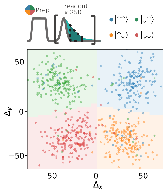
To measure the state of the nuclear spin we use the photon counting statistics obtained after sending a -pulse at each of the resonant frequencies , , and . We define , , and as the accumulated number of counts after applying a -pulse with frequency matching each of the electron spin transitions respectively. We then introduce
| (2) |
(resp. ) effectively "traces out" the state of Qb2 (resp. Qb1) as well as cancelling the contribution of the dark counts to the photon counting statistics. Figure 8 plots versus from the combined data presented in Fig. 1(d). The color of the points represents the state in which the system was prepared before the measurement took place. There are four well resolved distributions, each corresponding to a different prepared state of the two-nuclear-spin system. We use a -means algorithm to separate the space corresponding to each distribution, displayed in the plot with the corresponding background color. The boundaries approximately correspond to the and curves as expected. The skewness in the boundaries can be attributed to inaccurate calibration of the driving frequencies , , and , which would result in different counting statistics for each state. The main limiting factor for this scheme is the probability for a state to cross-relax. When the electron spin is excited, there is a non-negligible probability for the electron spin to subsequently decay through an electron-nuclear transition with probability proportional to , limiting the number of readout pulses that can be applied before the readout becomes non-QND. More details about the readout scheme can be found in [18]
Preparation into arbitrary nuclear spin states is done through a combination of sideband pumping (also known as solid-effect Dynamic Nuclear Polarization [28]) and single-qubit gates. Sideband pumping is achieved by driving the electron-nuclear transitions (represented as grey arrows in Fig. 1(b) of the main text) with a 3.5 ms length square pulse followed by 2 ms of wait time, allowing the electron spin to decay [18]. This sequence is then repeated 50 times to maximize the preparation efficiency. To prepare we drive the high frequency sidebands. To cover both Qb1 and Qb2 sidebands, the frequency of the pulse is chirped 50 kHz from + 760 kHz to + 810 kHz. To prepare other states, we apply the appropriate single-qubit gates after initializing in .
Appendix E SPAM errors
State Preparation And Measurement (SPAM) errors arise from the non-ideality of the preparation and measurement schemes and limit the performance of any quantum computing platform. These errors can be characterized and subsequently removed from the results of complex measurements, such as state tomography. One such method is the matrix SPAM correction technique [29]. The matrix has a dimension of , where is the size of the quantum register, in our case =2. Each column of the matrix represents the probability distribution measured after preparing in a specific state. To remove SPAM errors, the inverse of the matrix is applied to the results of any measurement. From the data presented in Fig. 1(d) we measure the following matrix:
| (3) |
SPAM correction was performed for every tomography measurement and all fidelity values given in the text account for this. Through SPAM correction we measure an increase of fidelity from 0.79 to 0.88 for the state and an increase from 0.73 to 0.79 for the state.
Further study of the errors at play in the system will require the use of randomized benchmarking, which was not performed in the current experiment due to time constraints.
Appendix F Stimulated Raman driving of nuclear spins

In this section we derive the analytical expressions for the Rabi frequency of the Raman drive and the corresponding ac-Zeeman shifts for the Hamiltonian presented in Eq. II. The corresponding energy levels are shown in Fig. 9. In the sketched diagram, the system is under drive by two off-resonant tones in order to induce a stimulated Raman transition in Qb2. The two tones have amplitudes and , defined with respect to the Rabi frequency of the electron at the same microwave amplitude :
| (4) |
where is the magnetic field at resonance generated by the nanowire under drive. The second term in the expressions for originates from the filtering of the resonator, with linewidth kHz. is experimentally obtained by rescaling the Rabi frequency presented in Fig. 7(d) by the respective drive amplitudes. In Fig. 9, both tones are shown twice for each state of Qb1. Let us restrict ourselves to the subset of levels where Qb1 is in the state. When the frequency difference between the two drives is equal to , the Qb2 is coherently driven from one state to the other following Rabi oscillations. Due to the presence of two excited states, two possible virtual paths need to be taken into consideration, the strength of each is given by
| (5) |
where the second term accounts for the driving of the sideband transition, which changes the corresponding matrix element. The addition of the two paths yields the total strength of the Raman drive
| (6) |
We now proceed to derive the ac-Zeeman shift . The presence of these two off resonant drives will inevitably induce ac-Zeeman shifts on the energy levels, which will in turn change the resonance condition for the spontaneous Raman transition from to (resp. ) if Qb1 is in state (resp. ). In the high field limit, where the shifts can be directly calculated as the combined shift of each drive on every electron transition,
| (7) |
where and . We introduce the following quantities: and . measures the relative ac-Zeeman shift on Qb2 depending on the state of Qb1. A single-qubit gate on Qb2 requires so that the drive is completely independent of the state of Qb1. This can be achieved by matching the two drive amplitudes and setting the appropiate value of . To calculate the latter we solve for , which reduces to
| (8) |
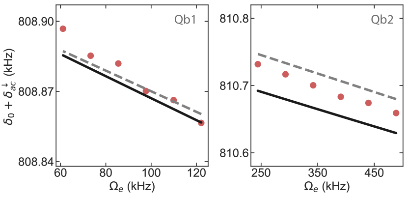
This third order polynomial always has a real root. At zero-order () we obtain , which amounts approximately to kHz as observed experimentally (Fig.2(d) of the main text).
For a two-qubit gate we try to maximize the value of . We set kHz and . This asymmetry is introduced to help preserve the Raman regime ( and ) when the value of is reduced. For this condition we measure Hz.
Figure 10 plots as a function of the drive amplitude at the following conditions: MHz and . The analytic expressions as well as the simulations performed using the Qutip package show quantitative agreement.
Appendix G State Tomography
We define the fidelity of a measured state with respect to a target state as [30]
| (9) |
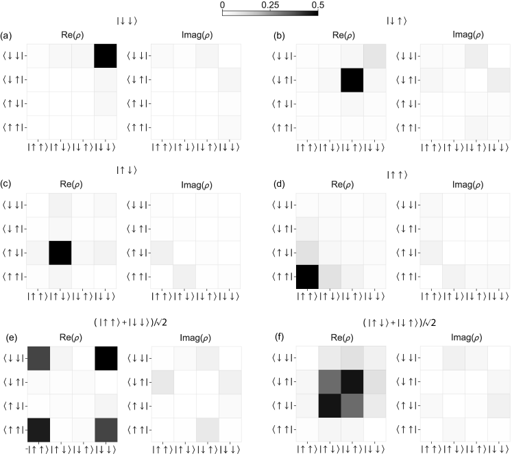
Figures 11(a,b,c,d) show the real and imaginary components of the tomographically reconstructed density matrices of the states , , , respectively. The fidelity for the single states is 0.99, 0.96, 0.9 and 0.93 respectively. has the highest fidelity compared to the other single states due to the state preparation protocol. As detailed in Appendix D, this is the initial state we prepare into via sideband pumping. The other states are prepared through single-qubit gates starting from .
Figures 11(e,f) show the real and imaginary components of the tomographically reconstructed density matrices of the Bell states and , respectively. We measure a comparatively reduced fidelity of 0.88 and 0.79 respectively. The reduction in fidelity likely originates from coherent errors on the single and two-qubit gates.
References
- Steger et al. [2012] M. Steger, K. Saeedi, M. L. W. Thewalt, J. J. L. Morton, H. Riemann, N. V. Abrosimov, P. Becker, and H.-J. Pohl, Quantum Information Storage for over 180 s Using Donor Spins in a 28Si “Semiconductor Vacuum”, Science 336, 1280 (2012).
- Zhong et al. [2015] M. Zhong, M. P. Hedges, R. L. Ahlefeldt, J. G. Bartholomew, S. E. Beavan, S. M. Wittig, J. J. Longdell, and M. J. Sellars, Optically addressable nuclear spins in a solid with a six-hour coherence time, Nature 517, 177 (2015).
- Pla et al. [2014] J. J. Pla, F. A. Mohiyaddin, K. Y. Tan, J. P. Dehollain, R. Rahman, G. Klimeck, D. N. Jamieson, A. S. Dzurak, and A. Morello, Coherent Control of a Single Si 29 Nuclear Spin Qubit, Phys. Rev. Lett. 113, 10.1103/PhysRevLett.113.246801 (2014).
- Muhonen et al. [2014] J. T. Muhonen, J. P. Dehollain, A. Laucht, F. E. Hudson, R. Kalra, T. Sekiguchi, K. M. Itoh, D. N. Jamieson, J. C. McCallum, A. S. Dzurak, and A. Morello, Storing quantum information for 30 seconds in a nanoelectronic device, Nat. Nanotechnol. 9, 986 (2014).
- Mądzik et al. [2022] M. T. Mądzik, S. Asaad, A. Youssry, B. Joecker, K. M. Rudinger, E. Nielsen, K. C. Young, T. J. Proctor, A. D. Baczewski, A. Laucht, V. Schmitt, F. E. Hudson, K. M. Itoh, A. M. Jakob, B. C. Johnson, D. N. Jamieson, A. S. Dzurak, C. Ferrie, R. Blume-Kohout, and A. Morello, Precision tomography of a three-qubit donor quantum processor in silicon, Nature 601, 348 (2022), publisher: Nature Publishing Group.
- Maurer et al. [2012] P. C. Maurer, G. Kucsko, C. Latta, L. Jiang, N. Y. Yao, S. D. Bennett, F. Pastawski, D. Hunger, N. Chisholm, M. Markham, D. J. Twitchen, J. I. Cirac, and M. D. Lukin, Room-Temperature Quantum Bit Memory Exceeding One Second, Science 336, 1283 (2012).
- Waldherr et al. [2014] G. Waldherr, Y. Wang, S. Zaiser, M. Jamali, T. Schulte-Herbrüggen, H. Abe, T. Ohshima, J. Isoya, J. F. Du, P. Neumann, and J. Wrachtrup, Quantum error correction in a solid-state hybrid spin register, Nature 506, 204 (2014), publisher: Nature Publishing Group.
- Bradley et al. [2019] C. E. Bradley, J. Randall, M. H. Abobeih, R. C. Berrevoets, M. J. Degen, M. A. Bakker, M. Markham, D. J. Twitchen, and T. H. Taminiau, A Ten-Qubit Solid-State Spin Register with Quantum Memory up to One Minute, Phys. Rev. X 9, 031045 (2019).
- Abobeih et al. [2022] M. H. Abobeih, Y. Wang, J. Randall, S. J. H. Loenen, C. E. Bradley, M. Markham, D. J. Twitchen, B. M. Terhal, and T. H. Taminiau, Fault-tolerant operation of a logical qubit in a diamond quantum processor, Nature 606, 884 (2022).
- Yu et al. [2024] X. Yu, B. Wilhelm, D. Holmes, A. Vaartjes, D. Schwienbacher, M. Nurizzo, A. Kringhøj, M. R. v. Blankenstein, A. M. Jakob, P. Gupta, F. E. Hudson, K. M. Itoh, R. J. Murray, R. Blume-Kohout, T. D. Ladd, A. S. Dzurak, B. C. Sanders, D. N. Jamieson, and A. Morello, Creation and manipulation of Schrödinger cat states of a nuclear spin qudit in silicon (2024), arXiv:2405.15494.
- Thiele et al. [2014] S. Thiele, F. Balestro, R. Ballou, S. Klyatskaya, M. Ruben, and W. Wernsdorfer, Electrically driven nuclear spin resonance in single-molecule magnets, Science 344, 1135 (2014).
- Godfrin et al. [2017] C. Godfrin, A. Ferhat, R. Ballou, S. Klyatskaya, M. Ruben, W. Wernsdorfer, and F. Balestro, Operating Quantum States in Single Magnetic Molecules: Implementation of Grover’s Quantum Algorithm, Physical Review Letters 119, 187702 (2017), publisher: American Physical Society.
- Bartling et al. [2024] H. P. Bartling, J. Yun, K. N. Schymik, M. v. Riggelen, L. A. Enthoven, H. B. v. Ommen, M. Babaie, F. Sebastiano, M. Markham, D. J. Twitchen, and T. H. Taminiau, Universal high-fidelity quantum gates for spin-qubits in diamond (2024), arXiv:2403.10633.
- Albertinale et al. [2021] E. Albertinale, L. Balembois, E. Billaud, V. Ranjan, D. Flanigan, T. Schenkel, D. Estève, D. Vion, P. Bertet, and E. Flurin, Detecting spins by their fluorescence with a microwave photon counter, Nature 600, 434 (2021).
- Lescanne et al. [2020] R. Lescanne, S. Deléglise, E. Albertinale, U. Réglade, T. Capelle, E. Ivanov, T. Jacqmin, Z. Leghtas, and E. Flurin, Irreversible Qubit-Photon Coupling for the Detection of Itinerant Microwave Photons, Phys. Rev. X 10, 021038 (2020), publisher: American Physical Society.
- Balembois et al. [2024] L. Balembois, J. Travesedo, L. Pallegoix, A. May, E. Billaud, M. Villiers, D. Estève, D. Vion, P. Bertet, and E. Flurin, Cyclically Operated Microwave Single-Photon Counter with Sensitivity of 10^\ensuremath-22\phantom\rule0.2em0ex\mathrmW/\sqrt\mathrmHz, Phys. Rev. Appl. 21, 014043 (2024), publisher: American Physical Society.
- Wang et al. [2023] Z. Wang, L. Balembois, M. Rančić, E. Billaud, M. Le Dantec, A. Ferrier, P. Goldner, S. Bertaina, T. Chanelière, D. Esteve, D. Vion, P. Bertet, and E. Flurin, Single-electron spin resonance detection by microwave photon counting, Nature 619, 276 (2023).
- Travesedo et al. [2024] J. Travesedo, J. O’Sullivan, L. Pallegoix, Z. W. Huang, P. Hogan, P. Goldner, T. Chaneliere, S. Bertaina, D. Esteve, P. Abgrall, D. Vion, E. Flurin, and P. Bertet, All-microwave spectroscopy and polarization of individual nuclear spins in a solid, ArXiv (2024), _eprint: 2408.14282.
- Bienfait et al. [2016] A. Bienfait, J. Pla, Y. Kubo, X. Zhou, M. Stern, C.-C. Lo, C. Weis, T. Schenkel, D. Vion, D. Esteve, J. Morton, and P. Bertet, Controlling Spin Relaxation with a Cavity, Nature 531, 74 (2016).
- Taminiau et al. [2012] T. H. Taminiau, J. J. T. Wagenaar, T. van der Sar, F. Jelezko, V. V. Dobrovitski, and R. Hanson, Detection and Control of Individual Nuclear Spins Using a Weakly Coupled Electron Spin, Phys. Rev. Lett. 109, 137602 (2012), publisher: American Physical Society.
- Leibfried et al. [2003] D. Leibfried, R. Blatt, C. Monroe, and D. Wineland, Quantum dynamics of single trapped ions, Reviews of Modern Physics 75, 281 (2003).
- [22] M. Le Dantec, M. Rančić, S. Lin, E. Billaud, V. Ranjan, D. Flanigan, S. Bertaina, T. Chanelière, P. Goldner, A. Erb, R. B. Liu, D. Estève, D. Vion, E. Flurin, and P. Bertet, Twenty-three-millisecond electron spin coherence of erbium ions in a natural-abundance crystal, Science Advances 7, eabj9786.
- Wang et al. [2024] Z. Wang, S. Lin, M. L. Dantec, M. Rančić, P. Goldner, S. Bertaina, T. Chanelière, R.-B. Liu, D. Esteve, D. Vion, E. Flurin, and P. Bertet, Month-long-lifetime microwave spectral holes in an erbium-doped scheelite crystal at millikelvin temperature (2024), arXiv:2408.12758.
- Abobeih et al. [2019] M. H. Abobeih, J. Randall, C. E. Bradley, H. P. Bartling, M. A. Bakker, M. J. Degen, M. Markham, D. J. Twitchen, and T. H. Taminiau, Atomic-scale imaging of a 27-nuclear-spin cluster using a single-spin quantum sensor, Nature 576, 411 (2019).
- Bartling et al. [2022] H. Bartling, M. Abobeih, B. Pingault, M. Degen, S. Loenen, C. Bradley, J. Randall, M. Markham, D. Twitchen, and T. Taminiau, Entanglement of Spin-Pair Qubits with Intrinsic Dephasing Times Exceeding a Minute, Physical Review X 12, 011048 (2022), publisher: American Physical Society.
- Majer et al. [2007] J. Majer, J. M. Chow, J. M. Gambetta, J. Koch, B. R. Johnson, J. A. Schreier, L. Frunzio, D. I. Schuster, A. A. Houck, A. Wallraff, A. Blais, M. H. Devoret, S. M. Girvin, and R. J. Schoelkopf, Coupling superconducting qubits via a cavity bus, Nature 449, 443 (2007).
- Antipin, A.A. et al. [1981] Antipin, A.A., Bumagina, L.A., Malkin, B.Z., and Rakhmatullin, R.M., Anisotropy of Er3+ spin-lattice relaxation in LiYF4 crystals, Soviet Journal of Experimental and Theoretical Physics 23, 2700 (1981).
- Abragam, A., Procto, W. [1958] Abragam, A., Procto, W., Une nouvelle méthode de polarisation des noyaux atomiques dans les solides, C.R. Acad. Sci. Paris , 2253 (1958), edition: 246.
- Lidar and Brun [2013] D. Lidar and T. Brun, Quantum Error Correction (Cambridge University Press, 2013).
- Nielsen and Chuang [2010] M. A. Nielsen and I. L. Chuang, Quantum Computation and Quantum Information: 10th Anniversary Edition (Cambridge University Press, 2010).