WAND: Wavelet Analysis-based Neural Decomposition of MRS Signals for Artifact Removal

Abstract

[Abstract] Accurate quantification of metabolites in mrs is challenged by low snr (snr), overlapping metabolites, and various artifacts. Particularly, unknown and unparameterized baseline effects obscure the quantification of low-concentration metabolites, limiting mrs reliability. This paper introduces wand (wand), a novel data-driven method designed to decompose MRS signals into their constituent components: metabolite-specific signals, baseline, and artifacts. wand takes advantage of the enhanced separability of these components within the wavelet domain. The method employs a neural network, specifically a U-Net architecture, trained to predict masks for wavelet coefficients obtained through the continuous wavelet transform. These masks effectively isolate desired signal components in the wavelet domain, which are then inverse-transformed to obtain separated signals. Notably, an artifact mask is created by inverting the sum of all known signal masks, enabling wand to capture and remove even unpredictable artifacts. The effectiveness of wand in achieving accurate decomposition is demonstrated through numerical evaluations using simulated spectra. Furthermore, wand’s artifact removal capabilities significantly enhance the quantification accuracy of linear combination model fitting. The method’s robustness is further validated using data from the 2016 MRS Fitting Challenge and in-vivo experiments.

1 Introduction

Nuclear mrs allows non-invasive determination of metabolite concentrations in biochemical samples of interest, making it a promising tool for diagnosing and monitoring various diseases, including cancer, neurological disorders, as well as traumatic brain injuries. ^{1, 2, 3, 4} However, clinical adoption is hindered by spectral quality issues, resulting from intrinsic low snr, artifacts, unknown baseline contributions, and other background signals. ⁵ Furthermore, overlapping metabolites and limited spectral resolution, even at high field strengths, can affect the reliability of metabolite quantification. ⁶ Consequently, human experts are often required, acquisition times are prolonged, and experiments need to be repeated. ⁷ These challenges have led to the development of various methods to enhance spectral quality, ranging from numerous model-based approaches to more recently introduced data-driven models ⁸.

Among these methods are traditional denoising techniques such as hsvd (hsvd) ⁹ and time-frequency transform-based techniques ^{10, 11, 12}, which focus on transforming the data to isolate and remove noise, or sliding window methods ⁹ that smooth the data by averaging neighboring points. These approaches have the drawback of over-smoothing the signals, thereby removing relevant information and obscuring quantification accuracy. Another conventional approach involves using total variation regularization for mrs ¹³ to reduce noise while maintaining sharp signal transitions. ¹⁴ This technique defines denoising as an optimization problem with the goal of finding a signal approximation that minimizes the total variation, e.g. the sum of squared errors. ¹³ However, computational complexity is high and the approach’s effectiveness depends on the optimal selection of the regularization parameter. ¹⁵

Alternatively, several deep learning techniques have been developed for data-driven denoising in mrs, particularly using U-Net architectures ^{16, 17, 18}, autoencoders ^{19, 20}, lstm networks ²¹, and vision transformers ¹⁸ to predict high snr data from low-quality measurements. Although deep learning-based denoising has shown promising results in various applications, its data-dependency and black-box nature make it difficult to interpret the outcome and rely on the denoising process.

In addition to denoising, the detection and removal of artifacts is crucial to accurately estimate metabolite concentrations ²² and improve the reliability and repeatability of experiments ⁵. There has been recent progress in data-driven quality filtering ^{23, 24} and artifact detection ^{25, 26, 27, 28}, however, the removal of artifacts remains more challenging. An autoencoder has been proposed ²⁶ to remove ghosting artifacts, also called spurious echoes, operating similarly to the denoising techniques ^{19, 20} by predicting clean data from corrupted data. An alternative approach ²⁹ was introduced to remove any artifact by employing a cnn (cnn) architecture, taking contaminated spectra as input and predicting noise-free, metabolite-only spectra. However, these methods work directly and without oversight on the spectra, potentially altering them significantly. This can restrict the available fitting parameter space leading to systemic quantification offsets or even directly introduce metabolite concentration biases.

Wavelet analysis is commonly used as a signal quality enhancement technique and has shown promise in characterizing mrs signals, capable of disentangling overlapping signal components and thereby removing noise, artifacts, and baseline contributions. ^{30, 31} The basic principle of the wavelet transform is to represent a signal as a set of basis functions called wavelets. Common denoising techniques include wavelet thresholding and wavelet shrinkage. Wavelet thresholding ^{32, 33} involves zeroing out coefficients below a specific threshold, thereby eliminating noise or other unwanted components. In contrast, wavelet shrinkage ^{34, 35} reduces the magnitude of the wavelet coefficients, leading to more robust data representation and noise reduction. In the context of mrs, wavelet transform has been used for various purposes ³⁶, such as quantification of signal parameters ³⁰, or characterization of non-parameterizable signal components ³⁷, including baseline ³⁸ and macromolecular contributions ³¹. A recent data-driven method ³⁹ employed a svm to classify coefficients to selectively remove noise components while preserving metabolite peaks. This exploits the enhanced separability of mrs signal components in the wavelet domain through a sample-adaptive approach. Nevertheless, metabolite signals exhibit high-frequency components that overlap with each other and noise, even within the wavelet domain. This is particularly pronounced at points of abrupt signal changes, necessitating a more flexible technique.

This work introduces the wand, a novel physics-driven method for decomposing signals into desired individual components. By combining the power of wavelet analysis and the adaptability of neural networks, we achieve a comprehensive breakdown of mrs signals into their metabolite-specific, baseline, and artifact components. This enables the targeted removal of unwanted signal components, such as artifacts and baseline contributions, while preserving the integrity of the desired metabolite signals, ultimately leading to more accurate and reliable metabolite quantification. The proposed wand architecture features a U-Net that predicts soft masks for the wavelet coefficients derived from the cwt (cwt) of the signal. These masks are used to isolate the desired signal components in the wavelet domain, which are then inverse-transformed to obtain the separated signals. The network is optimized with simulated mrs spectra using the mse (mse) of predicted and ground truth decompositions. Additionally, an artifact mask for unknown and non-parametrizable signals is created by inverting the sum of all known signals and ensuring complete coverage of the wavelet coefficients with a softmax function. This process yields a mask for unpredictable signals which can be used to remove unknown and random artifacts from mrs signals. Numerical results with simulated spectra demonstrate an accurate decomposition, with mse values of predicted and ground truth decompositions ranging from 2.32e-4 (± 1.2e-5) to 1.74e-6 (± 4.9e-8) for the normalized real components. The artifact removal capabilities significantly enhance the quantification accuracy of linear combination fitting. We further validate the wand’s effectiveness using data from the 2016 MRS Fitting Challenge ^{40, 41} and in-vivo experiments.

The rest of the article is organized as follows: Section 2 describes the assumed signal model and introduces the wavelet transform; Section 3 introduces the proposed wand, including details on neural architecture and training; Section 4 introduces the simulated and in-vivo data; Section 5 presents the results; Section 6 and Section 7 provide a discussion and concluding remarks.

2 System Model & Preliminaries

In this section, we detail the system model for which we train the wand and introduce other prerequisites. With that aim, we first present the assumed mrs signal model as well as the noise and artifact generation in Section 2.1. Then, we formulate the cwt and discuss its application to mrs in Section 2.2.

2.1 Signal Model

The chosen mrs signal model follows the form of a standard Voigt-lineshaped model ⁴²:

$$S_{m}(f)=e^{i(\phi_{0}+f\phi_{1})}a_{m}\mathcal{F}\{s_{m}(t)\ e^{-(\gamma+\varsigma^{2}t+i\epsilon)t}\},$$ (1)

$$X(f)=\sum^{M}_{m=1}S_{m}(f)+B(f)+R(f)+P(f)+N,$$ (2)

where $\phi_{0}$ and $\phi_{1}$ are the zero and first-order phases, the $a_{m}$ are the concentrations of the $M$ metabolites of interest, $\gamma$ and $\varsigma$ are Lorentzian and Gaussian broadening, respectively, and $\epsilon$ represents a frequency shift. $\mathcal{F}\{\cdot\}$ denotes the Fourier transform and the basis functions $\{s_{m}(t)\}_{m=1}^{M}$ are the full spectral contributions of the individual metabolites, obtained using density matrix simulations ^{43, 44}. mm are included, experiencing the same broadening, phasing, and shifting as the metabolites. Furthermore, the baseline $B(f)$ is represented by a complex second-order polynomial, while $R(f)$, $P(f)$, and $N$ correspond to spectral distortions in form of random baselines, peaks, and awgn, respectively. The random walk ⁴⁵ $R(f)$ starts with a random initialization at $R(0)$ and takes steps of a given size in a random direction followed by a smoothing of the generated line that is bounded by a defined minimum and maximum. It is drawn separately for real and imaginary parts. The Gaussian peaks $P(f)$ are obtained as follows:

$$P(f)=\sum^{M+K}_{k=M+1}\mathcal{H}\{a_{k}e^{-\frac{(f-\epsilon_{k})^{2}}{2\varsigma_{k}^{2}}}\}e^{-i\phi_{0,k}},$$ (3)

with $K$ being the number of peaks and $\mathcal{H}\{\cdot\}$ representing the Hilbert transform.

2.2 Continuous Wavelet Transform

The principle of wavelet analysis ^{46, 47, 48, 49} is to represent a signal as a superposition of wavelets which are generated from a single mother wavelet through the process of scaling and translating the signal. ⁵⁰ The forward cwt is defined as:

$$W(s,\delta)=\frac{1}{\sqrt{s}}\int X(f)\Psi^{*}\left(\frac{f-\delta}{s}\right)\,df,$$ (4)

where $s$ corresponds to the scale factor, $\delta$ is the translation parameter, and $\Psi(f)$ represents the mother wavelet (with ^∗ denoting its complex conjugate). ⁵¹ This transformation yields a two-dimensional representation of the signal called scalogram $|W(s,\delta)|$. ⁵² The icwt (icwt) allows reconstruction of the signal and is obtained by integrating over all scales and translations of the wavelet coefficients:

$$X(f)=C_{\Psi}^{-1}\iint W(s,\delta)\frac{1}{\sqrt{s}}\Psi\left(\frac{f-\delta}{s}\right)\,d\delta\,ds,$$ (5)

with the admissibility constant $C_{\Psi}$ depending only on the wavelet $\Psi$. ⁵³ Due to the high redundancy of the transform many reconstruction formulas exist, and with the assumption of $\Psi$ being analytic and $X(f)$ real, we can simplify (5) to

$$X^{\Re}(f)=\Re\left\{C_{\Psi}^{-1}\int W(s,\delta)s^{-3/2}\,ds\right\},$$ (6)

with $\Re\{\cdot\}$ representing the real part. ^{54, 55}

Figure 1 shows the real part of an example spectrum $X^{\Re}(f)$ alongside its corresponding scalogram $|W^{\Re}(s,\delta)|$ as well as a selection of basis spectra $S_{m}^{\Re}(f)$ with their respective scalograms. Throughout this work, we employ the popular Morlet wavelet ⁵¹ and apply the wavelet transform in the frequency domain to retain the well-known chemical shift axis for enhanced interpretability of the decomposition. Additionally, this allows truncation of the signal without losing any metabolite contributions by selecting only a relevant ppm range. Also, most mrs quantification methods utilize the frequency domain for lcm (lcm) ^{56, 57, 42}. However, it is not a necessity and the method also operates identically in the time domain.

3 Wavelet Analysis-based Neural Decomposition

The following sections introduce the proposed wand. Our approach achieves a data-driven decomposition of mrs signals into metabolite-specific, baseline, and artifact components by taking advantage of their enhanced separability in the wavelet domain. Particularly, we train a neural network to mask the wavelet coefficients to obtain the desired signal components in the wavelet domain and then subsequently inverse transform them to attain the separated signals. We next elaborate on the architecture of the wand in Section 3.1 and then present the training method in Section 3.2.

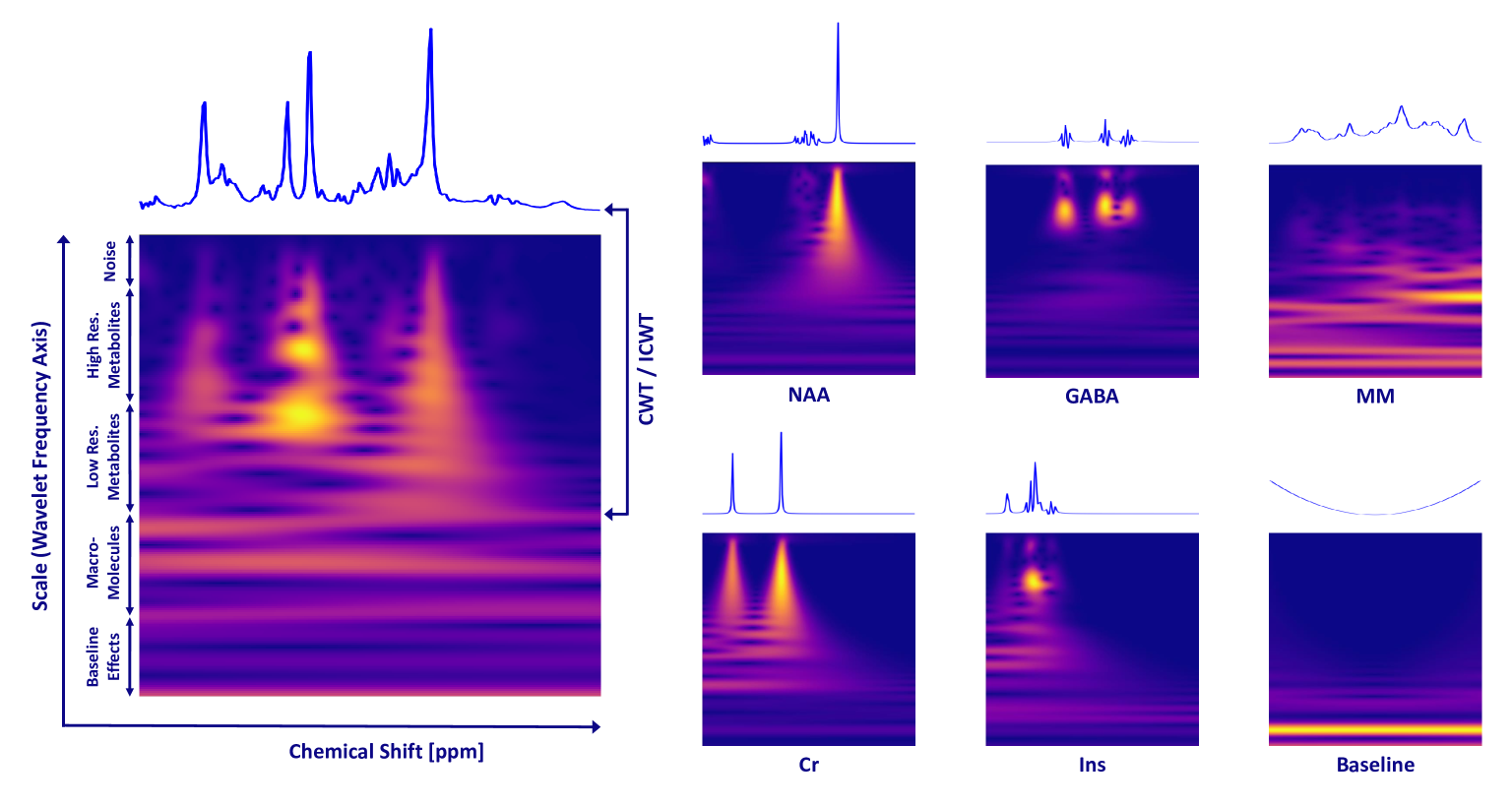
Figure 1: Depicts the real part of a simulated example mrs spectrum and its associated cwt, along with spectra and scalograms of various metabolites and other signal components (naa, gaba, mm, cr, ins, and a baseline). The scalograms demonstrate the enhanced separation of the metabolite signals in the wavelet domain, effectively allowing separation between high-frequency noise, metabolites, mm, and other baseline components.

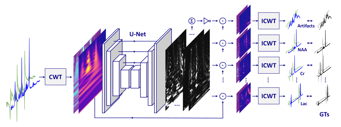
Figure 2: Schematic of the wand architecture. The proposed network produces soft masks for the signal’s real and imaginary components. These masks are applied to the wavelet coefficients, effectively isolating information specific to each metabolite. The resulting metabolite-specific scalograms can then be converted back into spectra using the icwt. An artifact mask is created by summing all the predicted masks and subsequently inverting them. A softmax function is applied to ensure that the sum of all resulting masks equals one, thereby achieving an absolute decomposition of the signal, which is compared to a ground truth decomposition.

3.1 Architecture

An overview of the wand architecture is detailed in Figure 2. The pipeline starts by individually transforming the relevant frequencies of the real and imaginary parts of the spectrum into their respective two-dimensional cwt representations. However, having a short signal with frequency extrema amplifies imperfections in the cwt filterbank resulting in an imperfect reconstruction with the icwt. ⁵⁵ To alleviate the issue of an underrepresented zeroth filterbank, we remove the DC component from the signal prior to computing the cwt. The effects of this on quantification are minimal and mostly depend on the initialization of the baseline modeling parameters of lcm methods. The stacked scalograms serve as an input to a U-Net, a cnn architecture that is particularly effective for image segmentation ⁵⁸, composed of an encoder and a decoder path with skip connections. See Appendix B, Table 4 for the specific neural network layer details. It outputs soft segmentation masks $\{H_{m}^{\Re}(s,\delta),H_{m}^{\Im}(s,\delta)\}_{m=1}^{M+1}\in[0,1]$ for both the real and imaginary parts of all considered metabolites and a baseline component. Furthermore, an artifact mask is obtained by summing and inverting all these masks for real and imaginary parts, i.e. $H_{M+2}^{\Re}=1-\sum_{m=1}^{M+1}H_{m}^{\Re}$ and $H_{M+2}^{\Im}=1-\sum_{m=1}^{M+1}H_{m}^{\Im}$. After which all masks are pushed through a softmax activation to ensure they sum to one, resulting in the complete coverage of the wavelet domain representation and an absolute decomposition of the signal in both the real and imaginary parts. Finally, the masks are applied to the wavelet coefficients creating component-specific wavelet domain representations that can be converted back to individual spectra using the icwt:

$$\begin{split}\hat{S}_{m}^{\Re}(f)&=\text{ICWT}\{W^{\Re}(s,\delta)\cdot H_{m}^{\Re}(s,\delta)\},\\ \hat{S}_{m}^{\Im}(f)&=\text{ICWT}\{W^{\Im}(s,\delta)\cdot H_{m}^{\Im}(s,\delta)\}.\end{split}$$ (7)

3.2 Training Strategy

Table 1: Overview of the notations and distribution ranges of the simulation parameters. The metabolite concentration ranges are taken from De Graaf 2019 ⁵⁹. $\mathcal{U}[a,b]$ and $\mathcal{U}\{a,b\}$ denote continuous and discrete uniform distributions, respectively.

Parameter	Notation	Range
Acetate (Ace)	$a_{1}$	$\mathcal{U}[0.0,0.5]$
Alanine (Ala)	$a_{2}$	$\mathcal{U}[0.1,1.6]$
Ascorbate (Asc)	$a_{3}$	$\mathcal{U}[0.4,1.7]$
Aspartate (Asp)	$a_{4}$	$\mathcal{U}[1.0,2.0]$
Creatine (Cr)	$a_{5}$	$\mathcal{U}[4.5,10.5]$
Gamma-Aminobutyric Acid (GABA)	$a_{6}$	$\mathcal{U}[1.0,2.0]$
Glycerophosphocholine (GPC)	$a_{7}$	$\mathcal{U}[0.4,1.7]$
Glutathione (GSH)	$a_{8}$	$\mathcal{U}[1.7,3.0]$
Glucose (Glc)	$a_{9}$	$\mathcal{U}[1.0,2.0]$
Glutamine (Gln)	$a_{10}$	$\mathcal{U}[3.0,6.0]$
Glutamate (Glu)	$a_{11}$	$\mathcal{U}[6.0,12.5]$
Glycine (Gly)	$a_{12}$	$\mathcal{U}[0.2,1.0]$
Myo-Inositol (Ins)	$a_{13}$	$\mathcal{U}[4.0,9.0]$
Lactate (Lac)	$a_{14}$	$\mathcal{U}[0.2,1.0]$
Macromolecules (MM)	$a_{15}$	$\mathcal{U}[0.0,10.0]$
N-Acetylaspartate (NAA)	$a_{16}$	$\mathcal{U}[7.5,12.0]$
N-Acetylaspartylglutamate (NAAG)	$a_{17}$	$\mathcal{U}[0.5,2.5]$
Phosphocholine (PCho)	$a_{18}$	$\mathcal{U}[0.2,1.0]$
Phosphocreatine (PCr)	$a_{19}$	$\mathcal{U}[3.0,5.5]$
Phosphoethanolamine (PE)	$a_{20}$	$\mathcal{U}[1.0,2.0]$
Taurine (Tau)	$a_{21}$	$\mathcal{U}[3.0,6.0]$
Scyllo-Inositol (sIns)	$a_{22}$	$\mathcal{U}[0.2,0.5]$

Parameter	Notation	Range
Number of Metabolites (+MM)	$M$	$\{22\}$
Frequency Shifts	$\epsilon$	$\mathcal{U}[-5,5]$
Lorentzian Broadening	$\gamma$	$\mathcal{U}[2,15]$
Gaussian Broadening	$\varsigma$	$\mathcal{U}[2,15]$
Zeroth-Order Phase	$\phi_{0}$	$\mathcal{U}[-0.2,0.2]$
First-Order Phase	$\phi_{1}$	$\mathcal{U}[-10^{-5},10^{-5}]$
Baseline Coefficients	$b_{1}$	$\mathcal{U}[-60,20]$
	$b_{2}$	$\mathcal{U}[-80,40]$
	$b_{3}$	$\mathcal{U}[-100,60]$
	$b_{4}$	$\mathcal{U}[-60,100]$
	$b_{5}$	$\mathcal{U}[-160,20]$
	$b_{6}$	$\mathcal{U}[-40,100]$
Random Walk Step Size		$\mathcal{U}[0,10^{3}]$
Random Walk Smoothing		$\mathcal{U}[1,10^{3}]$
Random Walk Min. Bound		$\mathcal{U}[-10^{4},0]$
Random Walk Max. Bound		$\mathcal{U}[0,10^{4}]$
Number of Peaks	$K$	$\mathcal{U}\{0,5\}$
Peak Amplitudes	$a_{M+1},...,a_{M+K}$	$\mathcal{U}[0,6\cdot 10^{4}]$
Peak Widths	$\varsigma_{M+1},...,\varsigma_{M+K}$	$\mathcal{U}[0,100]$
Peak Phases	$\phi_{M+1},...,\phi_{M+K}$	$\mathcal{U}[0,2\pi]$
Peak Locations	$\epsilon_{M+1},...,\epsilon_{M+K}$	$\mathcal{U}\{0,2048\}$
Complex Gaussian Noise∗	$N$	$\mathcal{CN}(0,500)$

snr ranging from 5 - 25 dB as computed from the ground truth metabolite and noise signals over 0.5 to 4.5 ppm.

The wand is trained end-to-end in a supervised setting as a regression problem with simulated mrs data. To increase data variability, we simulate each batch ad-hoc during training by drawing the signal model parameters from uniform distributions (see Table 1 for details) and employing equations (1) and (2) to obtain a batch of spectra $\{X_{u},Y_{u}\}_{u=1}^{U}$ with $U$ samples and ground truths $Y_{u}=(S_{1},...,S_{M},S_{M+1}=B,S_{M+2}=R+P+N)_{u}$, which hold the individual signal components before the summation in Equation (2). Note that we combine the contamination’s $R,P,N$ into on single artifact component $S_{M+2}$.

Having the ground truths of the simulations, we can compare the predicted decomposition $\hat{Y}_{u}$ with actual decomposition $Y_{u}$ via the mse of the individual spectra:

$$\begin{split}\mathcal{L}(Y_{u},\hat{Y}_{u})=\frac{1}{2(M+2)}(\sum_{m=1}^{M+2}\text{MSE}(S_{m}^{\Re}(f),\hat{S}_{m}^{\Re}(f))\\ +\sum_{m=1}^{M+2}\text{MSE}(S_{m}^{\Im}(f),\hat{S}_{m}^{\Im}(f))).\end{split}$$ (8)

The mse is computed over a defined frequency range, $f_{min}\leq f\leq f_{max}$, corresponding to 0.5 to 4.5 ppm throughout this work. After loss computation, we perform batch gradient descent using the Adam optimizer to update the weights of the U-Net via backpropagation through the architecture detailed in Figure 2. See Appendix B, Table 5 for a detailed overview of the relevant training parameters.

4 Materials & Methods

The following section introduces the data and analysis methods used to evaluate the performance of the proposed wand method. We utilize two different sets of artificial data and two different types of in-vivo data, as well as two different analysis methods for metabolite quantification with and without the use of wand for artifact removal.

4.1 Data Setup

The first type of simulated data is generated equally to the training data (described in Section 3.2) by drawing the signal parameters of equations (1) and (2) from uniform distributions as detailed in Table 1. This allowed the creation of a wide range of spectra with varying levels of metabolite concentrations, line broadening, phase shifts, and simulated artifacts.

The second set of artificial data consists of the 28 samples provided in the 2016 MRS Fitting Challenge data  ^{40, 41}. This data includes spectra with varying snr, lineshapes (Lorentzian and Voigt), linewidths, gaba and gsh concentrations, macromolecular contributions, artifacts such as eddy currents and residual water signals, as well as samples mimicking tumor spectra. ⁴¹ Both types were generated using the same basis set, based on the press (press) sequence with the following parameters: TE = 30 ms, TE1 = 11 ms, TE2 = 19 ms, TR >> T1, 123.22 MHz center frequency, 4000 Hz bandwidth, and 2048 spectral points.

The first in-vivo data samples are from the publicly available "fMRS in pain" data from Archibald et al. ⁶⁰, acquired at 3T with press and the following parameters: TE = 22 ms, TR = 4000 ms, 127.795 MHz center frequency, 2000 Hz bandwidth, and 2048 spectral points. We average the 15 baseline acquisitions for different nsa (nsa) to create spectra with varying levels of noise.

The second type of in-vivo data consists of spectra acquired from a healthy volunteer, who gave written informed consent, at Philips Medical System International B.V., Best, The Netherlands. It consists of two different voxel locations near the skull, with one voxel specifically chosen to include lipid contamination from subcutaneous fat. The acquisition parameters are: 3 T, press, TE = 30 ms, TR = 4000 ms, 127.75 MHz center frequency, 4000 Hz bandwidth, and 2048 spectral points. See Appendix C, Table 6 and 7, for the mrsinmrs (mrsinmrs) ⁶¹.

4.2 Processing & Analysis

The neural network of the proposed wand method is trained separately for each acquisition type by adjusting the basis set for the training data accordingly. Simulated data is used directly without any additional processing, as all necessary components are incorporated within the signal model. In contrast, the in-vivo data is processed using FSL-MRS (see mrsinmrs in Appendix B for details). Metabolite quantification is performed using two lcm fitting methods: FSL-MRS (Newton method) ⁴² and LCModel ⁵⁶. Fitting is conducted in the default range of LCModel, from 0.5 to 4.2 ppm, for all methods throughout this work. Furthermore, absolute quantification for the simulated data is obtained from relative metabolite concentration estimates $\{\hat{a}_{m}\}_{m=1}^{M}$ by optimally scaling to the absolute ground truth values $\{a_{m}\}_{m=1}^{M}$ using

$$w_{opt}=\min_{w}\sum_{m=1}^{M}\left|w\ \hat{a}_{m}-a_{m}\right|,$$ (9)

leading to an error computation via $\left|w_{opt}\ \hat{a}_{m}-a_{m}\right|$ for all metabolites $M$. This ensures an equal comparison of concentration estimates without a water reference or the influence of a single estimate, such as when referencing to e.g. tcr (tcr).

5 Results

In the following section, we present our experimental evaluations of the wand method. First, we showcase the achievable decompositions as well as benchmark wand against common denoising techniques on a synthetic test setup corresponding to the configurations of the training data ranges (Section 5.1); then analyze the potential to enhance quantification accuracy on the artificial data of the 2016 MRS Fitting Challenge ^{40, 41} (Section 5.2); and finally validate the robustness of wand on in-vivo experiments (Section 5.3 and Section 5.4).

5.1 Simulated Data

We first provide an overview of the input, intermediate, and output steps involved in the wand framework for the real component channels (the imaginary channels are placed in Appendix A, Figure 12). Figure 3 shows a randomly selected test spectrum alongside its scalogram. This is followed by the masks created by the U-Net and the separate scalograms obtained after applications of the masks to the input scalogram. The spectra resulting from the icwt of the decomposed scalograms are then displayed, along with the corresponding ground truth spectra of the individual metabolites for comparison. The predicted masks capture the fundamental signal attributes, including correct broadening, phase and frequency alignment.

Next, we present a more in-depth analysis of the complete decompositions achieved with wand. Figure 4 depicts the real parts of the predicted wand of four random example spectra alongside the corresponding ground truth decompositions in the chemical shift range of 0.5 to 4.5 ppm. The analogous decompositions of the imaginary parts are in Appendix A, Figure 13. The reconstruction error represents the residual (of the real part) of the original signal and the summed icwt reconstructions, i.e. $X-\sum_{m=1}^{M+2}S_{m}$, and arises from minor imperfections of the icwt, as discussed in Section 3.1. The metabolite signals are effectively isolated by wand, despite minor signal imperfections, resulting in Gaussian noise in the artifact channel that closely mirrors the actual ground truth noise signal.

To evaluate the accuracy of the predicted decomposition, we list the obtained mse values when comparing the predicted and ground truth signal components of the decompositions in Table 2. The mse is calculated separately for the real and imaginary parts of 1000 test sample spectra, which have amplitudes normalized to an absolute value of 1. The se (se) is indicated in brackets and alternative error metrics are provided in Appendix A, Table 3.

Table 2: mse (± se) of the real and imaginary parts of the predicted and ground truth signal components, computed over a test set of 1000 random samples (with spectra normalized to an absolute value of 1).

Component	MSE Real	MSE Imag
Ace	1.75e-6 (± 4.9e-8)	2.41e-6 (± 5.8e-8)
Ala	2.62e-6 (± 6.3e-8)	3.44e-6 (± 7.4e-8)
Asc	2.53e-6 (± 6.2e-8)	3.30e-6 (± 9.0e-8)
Asp	1.74e-6 (± 4.9e-8)	2.70e-6 (± 5.7e-8)
Cr	2.61e-5 (± 1.0e-6)	3.06e-5 (± 1.3e-6)
GABA	2.70e-6 (± 5.7e-8)	3.29e-6 (± 7.0e-8)
Glc	3.52e-6 (± 9.3e-8)	5.42e-6 (± 2.4e-7)
Gln	7.07e-6 (± 1.9e-7)	8.52e-6 (± 3.1e-7)
Glu	1.51e-5 (± 6.0e-7)	1.80e-5 (± 7.4e-7)
Gly	2.02e-6 (± 6.4e-8)	2.60e-6 (± 6.3e-8)
GPC	1.46e-5 (± 6.8e-7)	1.54e-5 (± 6.5e-7)
GSH	5.70e-6 (± 1.5e-7)	1.01e-5 (± 5.1e-7)
Ins	1.54e-5 (± 6.8e-7)	1.56e-5 (± 6.4e-7)
Lac	2.06e-6 (± 5.4e-8)	2.70e-6 (± 5.8e-8)
Mac	3.72e-5 (± 1.7e-6)	6.51e-5 (± 4.6e-6)
NAA	1.90e-5 (± 6.2e-7)	2.49e-5 (± 9.0e-7)
NAAG	1.09e-5 (± 4.1e-7)	1.17e-5 (± 4.5e-7)
PCho	1.09e-5 (± 4.6e-7)	1.27e-5 (± 5.4e-7)
PCr	2.01e-5 (± 8.3e-7)	2.74e-5 (± 1.2e-6)
PE	2.82e-6 (± 7.3e-8)	3.67e-6 (± 1.3e-7)
sIns	2.16e-6 (± 6.3e-8)	3.15e-6 (± 8.0e-8)
Tau	1.11e-5 (± 5.2e-7)	1.38e-5 (± 6.0e-7)
Baseline	8.21e-6 (± 2.4e-7)	8.03e-6 (± 2.4e-7)
Artifacts	2.32e-4 (± 1.2e-5)	4.85e-4 (± 3.6e-5)

Given the isolation of metabolite and artifact signals through the decomposition, we can remove the artifact signal component from the input spectrum to obtain a cleaned, artifact-free spectrum. Figure 5 depicts the achievable quality enhancement for the real and imaginary parts of the four random examples and additionally shows the quantification errors for LCModel and FSL-MRS with and without the use of wand for artifact removal. We utilize Equation (9) to obtain an optimal reference scaling from relative to absolute concentrations.

In Figure 6, we compare the performance of various processing and quantification methods over a test set of 100 sample spectra. Presented are the obtained mae and corresponding crlbp for FSL-MRS standalone, FSL-MRS in combination with wand for removal of artifacts, LCModel by itself, LCModel with wand, LCModel with a sliding Gaussian window for denoising, LCModel with sift (sift) ¹⁰, LCModel with hsvd ⁹, and LCModel with wavelet thresholding ¹¹. FLS-MRS quantification is strongly hindered by the artifact contributions in the signal, obtaining an average error of 1.92 (± 0.25), while in combination with wand it achieves an average error of 0.66 (± 0.11). LCModel has larger baseline modeling freedom and achieves an average error of 0.89 (± 0.10) without preprocessing of the spectra and an error of 0.60 (± 0.07) with wand. Furthermore, preprocessing the spectra with a Gaussian sliding window ⁹, sift ¹⁰, hsvd ⁹, or wavelet thresholding ¹¹ leads to average LCModel quantification errors of 0.79 (± 0.08), 0.78 (± 0.09), 0.78 (± 0.09), 0.75 (± 0.08) respectively.

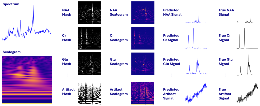
Figure 3: An illustrative summary of the steps involved within the wand framework, showcasing the real part of a random spectrum, its associated scalogram, several predicted masks, their respective masked scalograms, and the ultimately obtained spectral components along the corresponding ground truth signals.

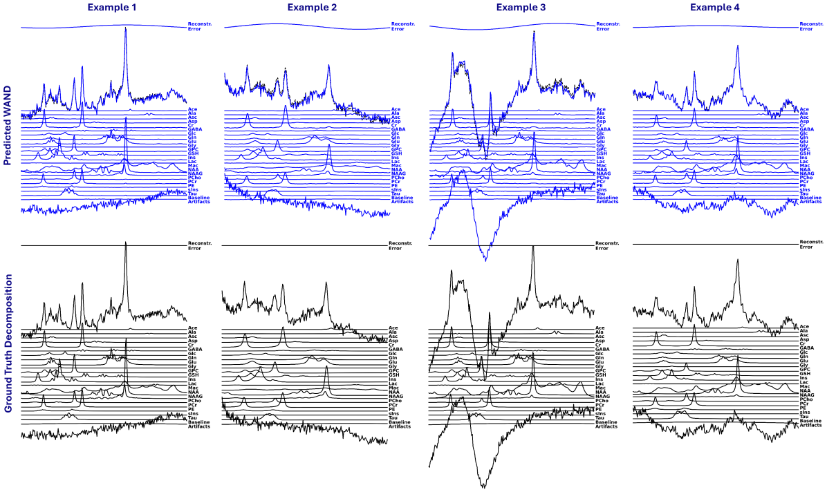
Figure 4: Shows the real parts of the complete predicted decomposition for four randomly selected examples, alongside their corresponding ground truth decompositions in the range of 0.5 to 4.5 ppm. The reconstruction error represents the residual of the original signal and the summed icwt reconstructions.

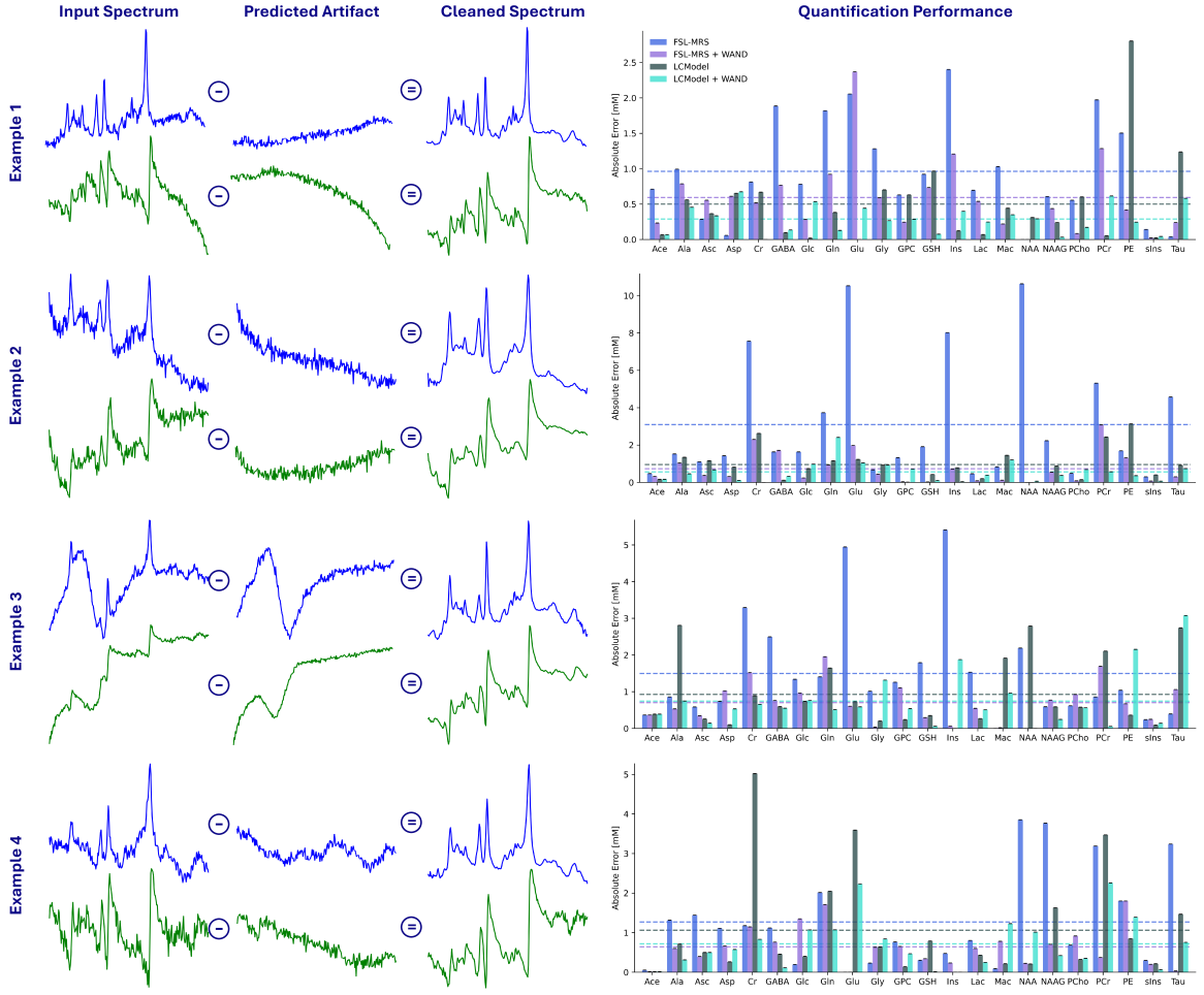
Figure 5: Depicts the real and imaginary parts of four example spectra, the predicted artifact component of the wand, and the cleaned signal obtained by subtracting the artifact. Alongside the visualizations, the absolute quantification errors per metabolite are shown when comparing the input spectra to the cleaned spectra for both FSL-MRS and LCModel (mae over all metabolites is provided through the dashed lines).

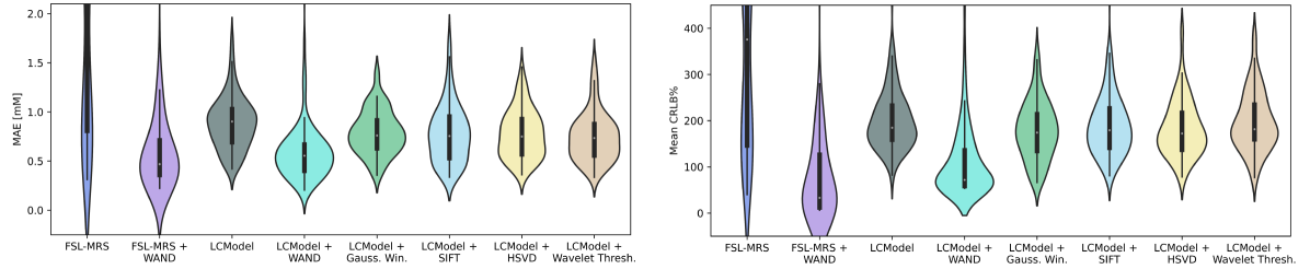
Figure 6: Comparison of the quantification mae and mean crlbp values over a test set of 100 samples for various methods: FLS-MRS standalone, FSL-MRS with wand, LCModel standalone, LCModel with wand, LCModel with a sliding Gaussian window, LCModel with sift, LCModel with hsvd, and LCModel with wavelet thresholding.

5.2 2016 MRS Fitting Challenge

In this section, we validate the results achieved with wand using the spectra of the 2016 MRS Fitting Challenge data set. Figure 7 provides an overview of the concentration estimates for selected metabolites, comparing the performance of standalone FSL-MRS and LCModel with their performance when combined with wand. Again, we utilize Equation (9) to obtain an optimal reference scaling from relative to absolute concentrations. The comparison highlights the impact of wand on refining the concentration estimates, providing a clearer understanding of the metabolites’ presence in the samples, particularly for cases with strong artifacts such as residual water. For gsh, we observed a systemic bias introduced by wand, likely due to its training range of 1.7 to 3 mM (see Table 1). However, it is noteworthy that a metabolite concentration of zero was correctly achieved in dataset samples 25, 26, and 28.

Figure 8 provides a detailed overview, listing the percentage error and crlbp values for all metabolites involved (excluding ace and mm) across the 28 challenge samples. Red corresponds to an overestimation and blue for an underestimation of the predicted concentrations compared to the ground truth concentrations. This figure highlights the concentration estimates obtained from FSL-MRS and LCModel, both independently and in conjunction with wand. Although biases appear when using wand, particularly for minor metabolites like ace, gsh, gly, and pe, we also observe a good correlation with the crlbp values and generally enhanced precision for other metabolites.

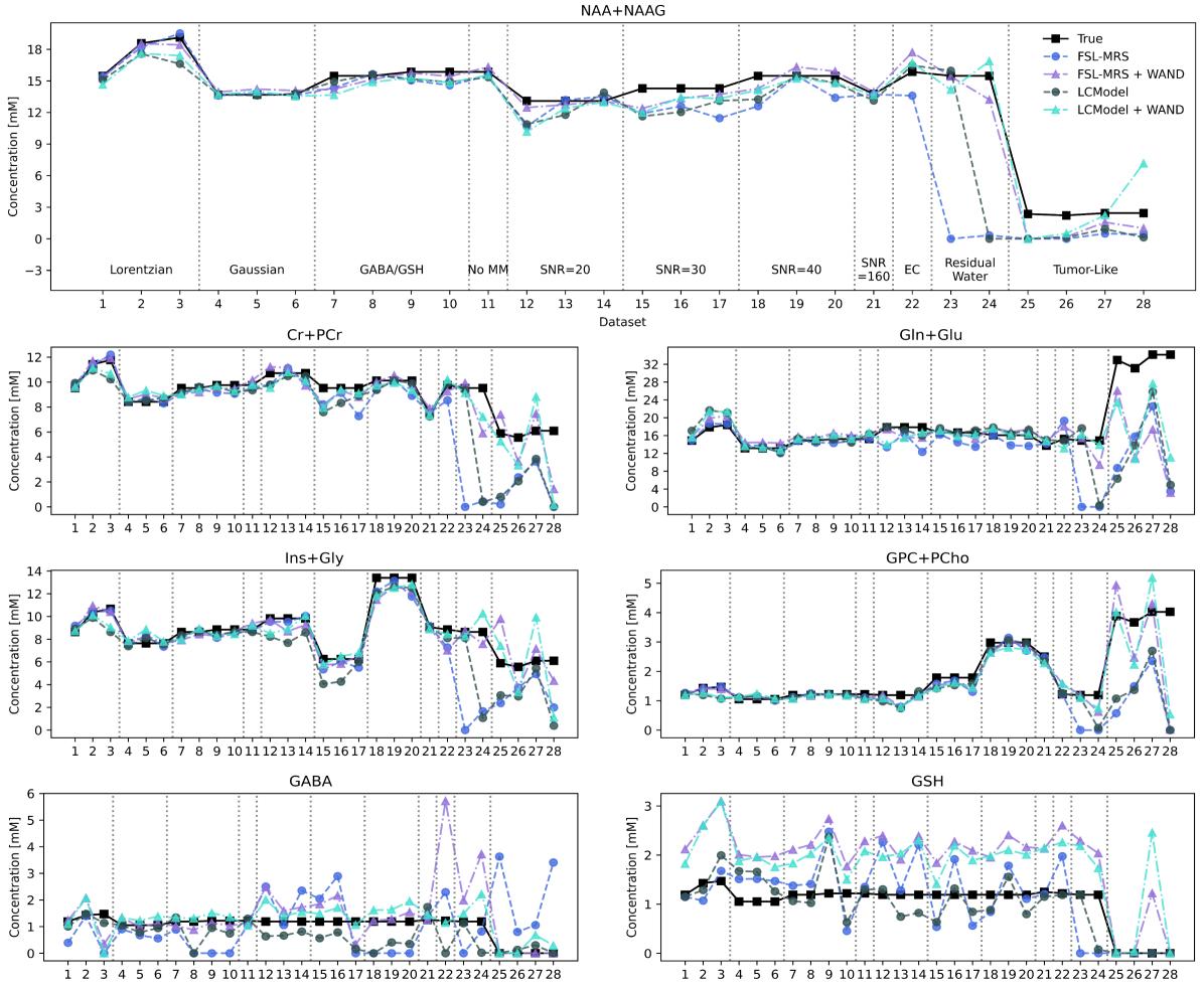
Figure 7: Comparison of standalone FSL-MRS and LCModel concentration estimates and in combination with wand processed spectra for each of the 28 samples of the 2016 MRS Fitting Challenge data set for selected metabolites.

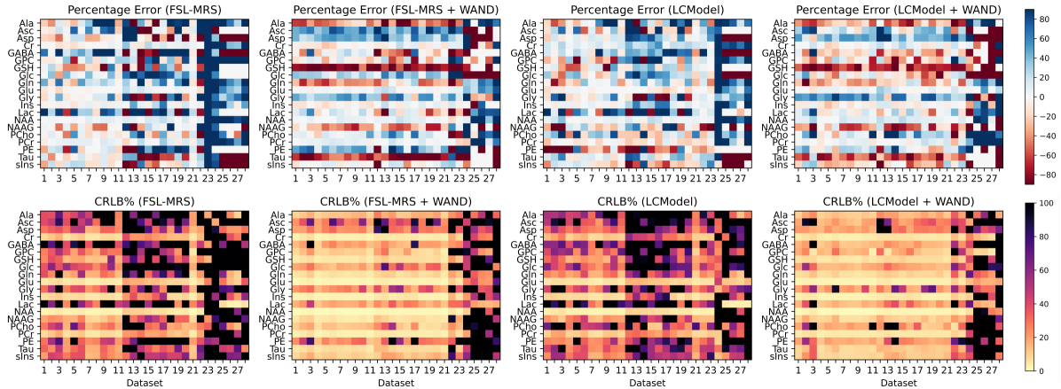
Figure 8: Depicts the obtained percentage error and crlbp values for all 28 challenge samples for all concentration estimates of FLS-MRS and LCModel alone as well as in combination with wand.

5.3 Noise Interference

To analyze the robustness of the wand method to in-vivo mrs data, we utilize the individual averages of the 15 baseline acquisitions of the "fMRS in pain" data. Specifically, we average the datasets for different nsa to obtain spectra of varying quality. Figure 9 shows, for dataset 3, the influence of noise interference on the estimated metabolite concentrations for FSL-MRS and LCModel, with or without wand processed spectra, for the major metabolites. Additionally, the metabolite concentration estimates reported in the work of Archibald et al. ⁶⁰ for 32 averages, obtained by LCModel, are included. The figure also presents the representative spectra, LCModel fits, and corresponding residuals for the different nsa, highlighting the influence of noise with or without the use of wand.

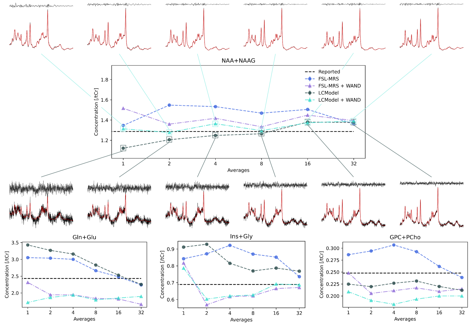
Figure 9: Shows the predicted metabolite concentration estimates of dataset 3 for varying NSA values using FSL-MRS and LCModel, with and without wand, for the major metabolites. Additionally, respective LCModel fits are displaced, showcasing the representative spectra, the model fit, and the residuals.

To further assess the reproducibility of the metabolite estimates with varying nsa, we computed the concordance correlation coefficients ⁶² between the reported major metabolite estimates for 32 averages and the obtained estimates for lower nsa using different methods. Figure 10 presents the obtained correlations for FSL-MRS and LCModel alone, as well as in combination with wand. It should be noted that the compared, reported values are LCModel estimates with a slightly different basis set. Therefore, we observe a strong correlation of nearly 1 at 32 averages for LCModel. In general, estimates when lcm are combined with wand show a stronger correlation throughout the lower nsa.

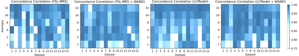
Figure 10: The obtained concordance correlation coefficients between the major metabolites reported ⁶⁰ and the obtained estimates of FLS-MRS and LCModel alone as well as in combination with wand for varying nsa.

5.4 Lipid Contamination

In this section, we examine the capability of wand to eliminate artifactual lipid signals originating from regions outside the brain ²². To achieve this, we first acquire a reference spectrum from a voxel near the skull. We then slightly adjust the voxel’s position closer to the skull to obtain a spectrum from nearly the same voxel, but with subcutaneous fat contamination. Figure 11 illustrates the exact voxel locations, the acquired spectra (with and without artifact removal using wand), the LCModel fits, and the respective metabolite quantifications. These quantifications highlight the difference between modeling the lipid signals with basis functions and removing them using wand. Additionally, we utilized the open-source database for in-vivo brain mrs ⁶³ to identify relevant literature values for metabolite concentrations of that brain region. The database was queried for healthy/control literature and filtered by subject age (over 18), TE of 30 ms, press sequence, proton mrs only, left brain side, and voxel location to minimize variability. This filtering resulted in the following literature ^{64, 65, 66, 67, 68}, from which metabolite concentrations were averaged, and a mean standard deviation was calculated. We notice a reasonable agreement with the literature for both methods, with slightly more constant concentration estimates obtained by applying the wand. However, the experiment is limited by only one sample, tissue composition, the influence of movement and displacement, processing of the spectra, as well as the analysis itself.

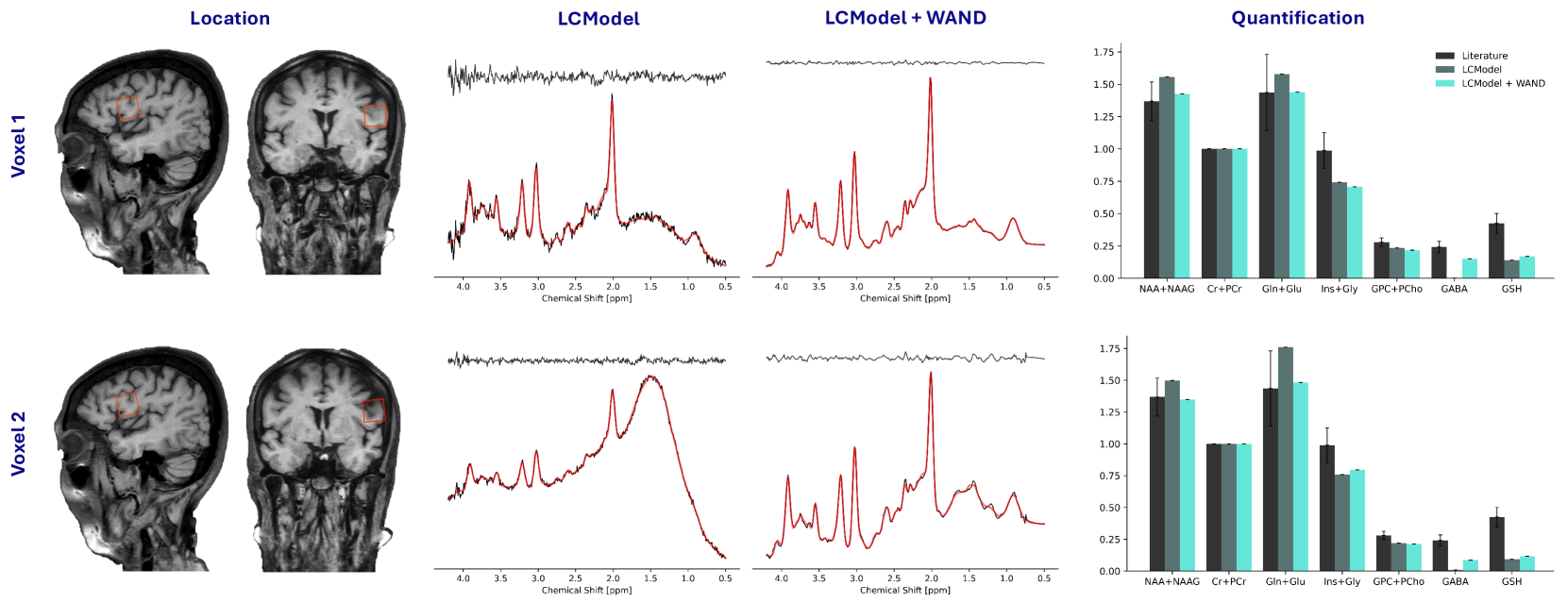
Figure 11: Acquired spectra, fitting, and quantification for two different voxel locations near the skull, with and without the use of wand for processing. Voxel 1 exhibits minimal influence from lipid signals originating outside the brain, whereas Voxel 2 is significantly affected by these artifacts.

6 Discussion

The proposed wand delivers an approach to adaptively categorize and separate wavelet coefficients with soft masks to account for overlapping signal structures. In contrast to traditional wavelet analysis methods for signal enhancement, such as sift ¹⁰, hsvd ⁹, or wavelet thresholding ¹¹ that separate signal and noise components in a hard manner. Furthermore, by creating an artifact mask from the residual of the measured signal signal and all known signal components the artifact channel is not predicted but inferred by predicting all other signal components. This allows wand to recover unpredictable random structures, such as Gaussian noise or signals generated by random walks.

The method demonstrates accurate decomposition in both simulated and in-vivo datasets, leading to significant improvements in quantification accuracy when combined with existing fitting methods like LCModel and FSL-MRS, as demonstrated in Figure 5. This is particularly evident in the case of spectra with strong artifacts, such as residual water signals in the 2016 MRS Fitting Challenge dataset or the lipid contaminations of Section 5.4, where wand preprocessing leads to refined concentration estimates.

While wand’s data-driven nature allows for adaptability, it can introduce biases, and relying solely on simulations during the training process may limit generalization capabilities. The accuracy of the decomposition heavily relies on the comprehensiveness of the simulated data and the distributions of the model parameters summarized in Table 1. Furthermore, the approach is trained for specific sequence parameters and is therefore dependent on these parameters to operate reliably, which is common for data-driven methods ⁸. However, wand offers significant advantages in terms of interpretability and reliability compared to conventional black-box deep learning methods. The decomposition of the mrs signal into its individual components allows for visual inspection, enabling users to directly assess the quality of artifact removal and the isolation of metabolite signals (Figures 3, 4, 5).

The combination of wand with least-squares fitting methods might not be optimal. As wand effectively removes Gaussian noise within the artifact component, the residual signal might no longer adhere to the Gaussian noise assumption inherent in least-squares methods. This could potentially impact the accuracy of quantification and might necessitate the exploration of alternative fitting approaches better suited for non-Gaussian residual noise.

Several areas for future research are important to consider. wand’s ability to identify and remove consistent baseline effects and artifacts across multiple measurements makes it particularly well-suited for fmrs (fmrs) applications. By applying the same baseline/artifact removal strategy to all time series data, wand can improve the accuracy of dynamic metabolite concentration estimates while only introducing potential systemic biases. Additionally, tailoring wand to specific applications, such as focusing on clinically relevant metabolites or specific types of artifacts, could further enhance its performance. This could be achieved by implementing a weighted loss function that prioritizes the accurate decomposition of specific metabolites or artifact patterns.

The choice of wavelet significantly impacts the decomposition process. Depending on the length, sparsity, and abruptness of signal changes, different wavelets are more suitable for distinguishing between signal and noise in the wavelet domain. ⁶⁹ In the case of wand, we encounter numerous components with varying frequency characteristics and different mean sparsity changes, making the selection of a single optimal wavelet impractical. Additionally, the artifact channel itself is highly variable, containing only noise at times, but also exhibiting smooth baseline signal changes and potential sharp water and lipid peak contaminations. Therefore, we compromise by selecting the computationally efficient Morlet wavelet as it has shown to be less sensitive to higher-order noise as well as baseline variation which allows for a more accurate separation of the metabolite signals from contaminations, and while preserving the integrity of the signals. ^{70, 71} Different wavelets may be more suitable depending on the specific characteristics of the signal being analyzed. Exploring adaptive wavelet methods ⁷² could lead to more robust and adaptable artifact removal strategies tailored to the specific features of individual MRS datasets.

Furthermore, investigating the potential of incorporating wand’s decomposed signal components as a basis set for quantification or augmenting existing basis sets with the artifact channel could be a promising direction for future research.

7 Conclusion

This paper introduced wand, a novel data-driven method for decomposing mrs signals into metabolite-specific, baseline, and artifact components. The method takes advantage of the enhanced separability of these components within the wavelet domain, using a U-Net architecture to predict soft masks for wavelet coefficients. These masks are then used to isolate and reconstruct individual signal components. wand demonstrated accurate decomposition performance on simulated spectra, as evidenced by the low mse values reported in Table 2 and the visualizations in Figures 3 and 4. Notably, wand’s ability to infer the artifact component by predicting all other signal components allows for the capture of unpredictable, random structures without explicit artifact modeling. The application of wand to both simulated and in-vivo data highlighted its potential to enhance the accuracy of metabolite quantification. By removing artifacts, wand improves the performance of linear combination model fitting, as shown in Figures 5, 6, 7, and 11. The method’s robustness is further supported by the improved concordance correlation coefficients observed when wand is combined with LCM methods for in-vivo data with varying noise levels (Figure 10).

Data Availability Statement

The source code used in our experiments for the method, data simulation, and analysis can be found at https://github.com/julianmer/WAND-for-MRS.

The Appendix of this paper is composed of three distinct sections: A Additional Materials, B Implementation Details, and C Minimum Reporting Standards in MRS. Each section contains supplementary information that aims to further enhance the workings and findings of the main text.

Appendix A Additional Materials

This appendix provides supplementary materials and analyses that support the findings and discussions presented in the main text.

• Figure 12 and Figure 13 present visualizations analogous to those shown in the main text (Figures 3 and 4), but focusing on the imaginary components of the wand framework.

• Table 3 expands upon the error analysis presented in Table 2 by providing a wider range of error metrics for the predicted signal decompositions.

• Figures14, 15, and 16 show metabolite concentration estimates for datasets 0, 5 and 10, analogous to Figure 9 which shows the same for dataset 3.

Figure 12: An illustrative summary of the steps in the wand, showcasing the imaginary part of the spectrum presented in Figure 3, its associated scalogram, several predicted masks, their respective applied scalograms, and the ultimately obtained spectral components along with the corresponding ground truth signals.

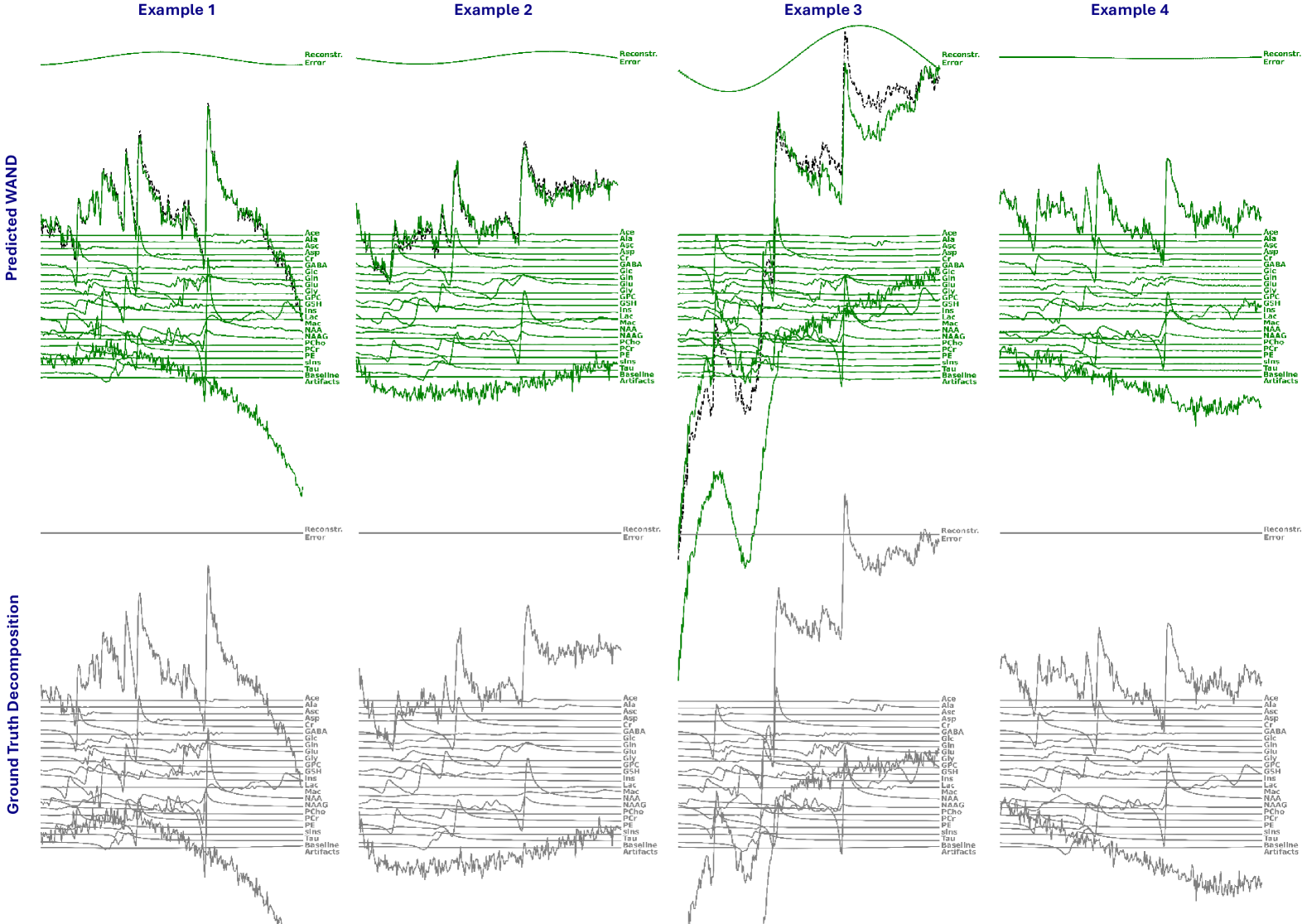
Figure 13: Shows the imaginary parts of the complete predicted decomposition for the four selected examples of Figure 4, alongside their corresponding ground truth decompositions in the range of 0.5 to 4.5 ppm.

Table 3: Unscaled mse, individually scaled component mse (each normalized to an absolute value of 1), and cosine similarity, as well as the se for all those measures (given in brackets with ±), of the real and imaginary parts of the predicted and ground truth signal components, computed over a test set of 1000 random samples.

Component	Un. MSE Real	Ind. MSE Real	Cos Sim. Real	Un. MSE Imag	Ind. MSE Imag	Cos Sim. Imag
Ace	1.95e+3 (± 1.9e+2)	7.11e-2 (± 3.4e-3)	0.68 (± 1.1e-2)	2.20e+3 (± 2.0e+2)	4.99e-2 (± 1.2e-3)	0.55 (± 9.0e-3)
Ala	2.13e+3 (± 2.0e+2)	4.49e-2 (± 2.6e-3)	0.78 (± 9.4e-3)	2.41e+3 (± 2.0e+2)	3.14e-2 (± 1.0e-3)	0.72 (± 8.4e-3)
Asc	2.08e+3 (± 1.9e+2)	4.56e-2 (± 2.6e-3)	0.82 (± 8.3e-3)	2.38e+3 (± 2.1e+2)	2.76e-2 (± 9.9e-4)	0.76 (± 8.4e-3)
Asp	1.95e+3 (± 1.9e+2)	6.37e-2 (± 3.0e-3)	0.73 (± 1.0e-2)	2.21e+3 (± 2.0e+2)	3.46e-2 (± 1.3e-3)	0.63 (± 9.7e-3)
Cr	6.44e+3 (± 3.1e+2)	6.63e-4 (± 4.7e-5)	0.99 (± 4.8e-4)	7.37e+3 (± 3.4e+2)	8.88e-4 (± 6.3e-5)	0.99 (± 5.5e-4
GABA	2.09e+3 (± 1.9e+2)	4.58e-2 (± 2.4e-3)	0.74 (± 9.7e-3)	2.26e+3 (± 1.9e+2)	3.15e-2 (± 1.4e-3)	0.74 (± 1.1e-2)
Glc	2.26e+3 (± 2.0e+2)	2.63e-2 (± 1.8e-3)	0.89 (± 6.8e-3)	2.63e+3 (± 2.0e+2)	2.02e-2 (± 8.8e-4)	0.86 (± 6.6e-3)
Gln	2.86e+3 (± 1.9e+2)	1.44e-2 (± 9.5e-4)	0.93 (± 4.1e-3)	3.23e+3 (± 2.1e+2)	8.19e-3 (± 4.7e-4)	0.93 (± 4.3e-3)
Glu	4.69e+3 (± 2.6e+2)	4.02e-3 (± 2.9e-4)	0.98 (± 1.6e-3)	5.10e+3 (± 2.5e+2)	2.73e-3 (± 1.7e-4)	0.98 (± 1.2e-3)
Gly	2.00e+3 (± 1.9e+2)	5.21e-2 (± 2.9e-3)	0.77 (± 9.5e-3)	2.23e+3 (± 2.0e+2)	2.88e-2 (± 1.0e-3)	0.73 (± 8.2e-3)
GPC	4.16e+3 (± 2.3e+2)	2.71e-3 (± 2.5e-4)	0.97 (± 1.9e-3)	4.42e+3 (± 2.3e+2)	2.97e-3 (± 2.8e-4)	0.97 (± 2.1e-3)
GSH	2.68e+3 (± 1.9e+2)	7.31e-3 (± 6.3e-4)	0.94 (± 3.6e-3)	3.37e+3 (± 2.1e+2)	8.82e-3 (± 5.7e-4)	0.93 (± 3.8e-3)
Ins	4.70e+3 (± 2.4e+2)	1.87e-3 (± 1.2e-4)	0.98 (± 8.7e-4)	4.87e+3 (± 2.7e+2)	2.90e-3 (± 2.2e-4)	0.98 (± 1.1e-3)
Lac	2.01e+3 (± 1.9e+2)	6.45e-2 (± 3.0e-3)	0.69 (± 1.0e-2)	2.28e+3 (± 2.0e+2)	4.58e-2 (± 1.2e-3)	0.62 (± 9.3e-3)
Mac	1.04e+4 (± 5.9e+2)	6.64e-3 (± 4.8e-4)	0.97 (± 2.4e-3)	1.47e+4 (± 8.3e+2)	3.31e-3 (± 2.3e-4)	0.99 (± 1.0e-3)
NAA	5.59e+3 (± 2.7e+2)	3.75e-4 (± 2.6e-5)	0.99 (± 3.7e-4)	6.41e+3 (± 3.1e+2)	7.95e-4 (± 1.0e-4)	0.99 (± 3.9e-4
NAAG	3.57e+3 (± 2.1e+2)	9.60e-3 (± 9.0e-4)	0.92 (± 4.4e-3)	3.76e+3 (± 2.1e+2)	8.70e-3 (± 5.9e-4)	0.93 (± 3.9e-3)
PCho	3.43e+3 (± 2.0e+2)	6.92e-3 (± 7.0e-4)	0.94 (± 3.9e-3)	3.83e+3 (± 2.2e+2)	6.90e-3 (± 5.0e-4)	0.93 (± 3.9e-3)
PCr	5.12e+3 (± 2.4e+2)	1.39e-3 (± 1.0e-4)	0.98 (± 9.2e-4)	6.12e+3 (± 2.5e+2)	1.71e-3 (± 1.3e-4)	0.98 (± 1.1e-3)
PE	2.10e+3 (± 1.9e+2)	4.19e-2 (± 2.3e-3)	0.82 (± 8.0e-3)	2.35e+3 (± 2.0e+2)	2.77e-2 (± 1.0e-3)	0.79 (± 8.1e-3)
sIns	2.02e+3 (± 1.9e+2)	2.65e-2 (± 2.1e-3)	0.86 (± 7.2e-3)	2.32e+3 (± 2.0e+2)	1.71e-2 (± 8.7e-4)	0.83 (± 7.1e-3)
Tau	3.66e+3 (± 2.2e+2)	7.07e-3 (± 6.5e-4)	0.97 (± 2.1e-3)	4.20e+3 (± 2.3e+2)	4.78e-3 (± 3.7e-4)	0.97 (± 2.0e-3)
Baseline	2.95e+3 (± 1.9e+2)	1.11e-1 (± 2.9e-3)	0.37 (± 1.7e-2)	3.07e+3 (± 2.1e+2)	1.52e-1 (± 3.1e-3)	0.19 (± 1.8e-2)
Artifacts	1.05e+5 (± 1.3e+4)	1.91e-3 (± 7.6e-5)	0.98 (± 7.7e-4)	1.35e+5 (± 1.1e+4)	2.22e-3 (± 7.1e-5)	0.98 (± 6.6e-4)

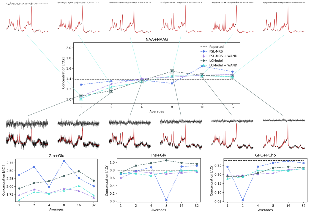
Figure 14: Shows the predicted metabolite concentration estimates of dataset 1 for varying NSA values using FSL-MRS and LCModel, with and without wand, for the major metabolites.

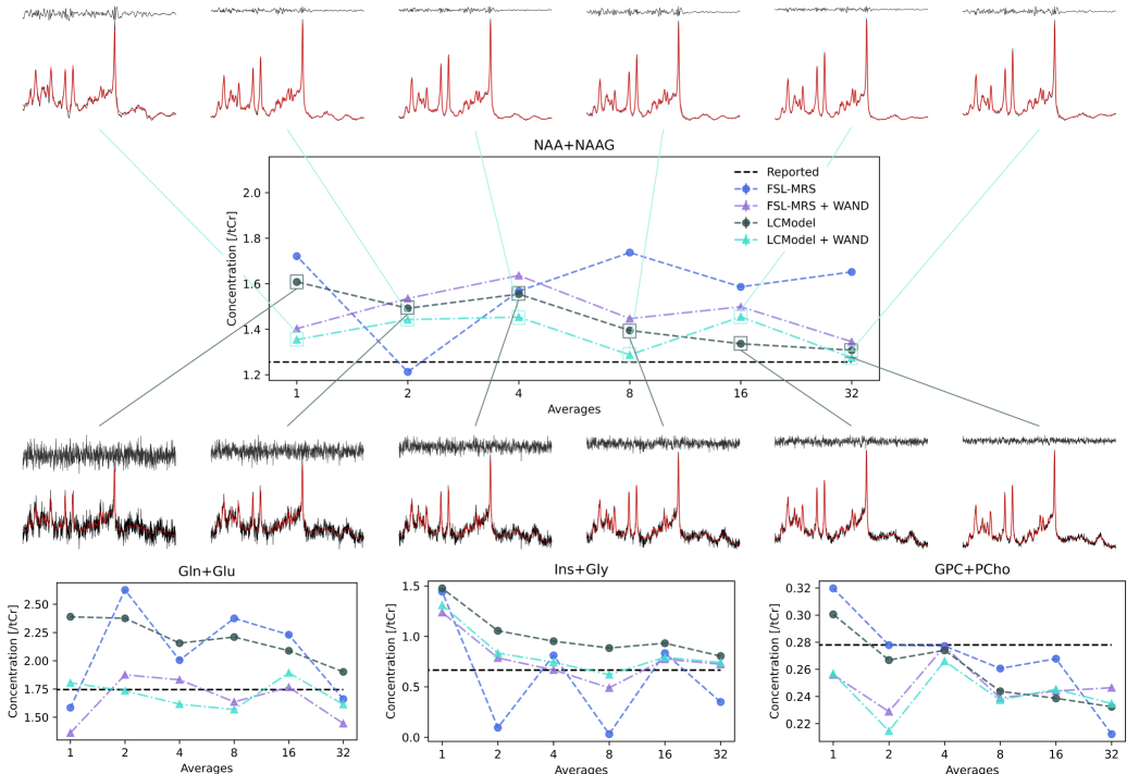
Figure 15: Shows the predicted metabolite concentration estimates of dataset 6 for varying NSA values using FSL-MRS and LCModel, with and without wand, for the major metabolites.

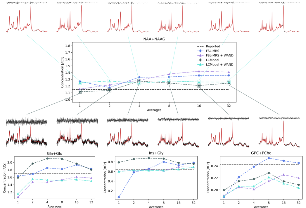
Figure 16: Shows the predicted metabolite concentration estimates of dataset 11 for varying NSA values using FSL-MRS and LCModel, with and without wand, for the major metabolites.

Appendix B Implementation Details

This section offers a closer look at the specific implementation choices made in developing the wand method.

• Table 4 dissects the U-Net architecture employed in wand, outlining the specific details of each layer within the network.

• Table 5 summarizes the settings and training parameters of the wand framework: This table serves as a quick reference guide for the various settings and hyperparameters used during the training and operation of the WAND framework.

Table 4: Specific neural network layer details of the U-Net architecture of wand implemented in PyTorch.                                                                                                        

Layer∗	Operation	Kernel Size	Stride	Padding	In Channels	Out Channels
Input	-	-	-	-	n_channels	-
DoubleConv	Conv2d, BN, ReLU	3	1	1	n_channels	64
	Conv2d, BN, ReLU	3	1	1
Down	MaxPool2d	2	2	0	64	128
	DoubleConv	3	1	1
Down	MaxPool2d	2	2	0	128	256
	DoubleConv	3	1	1
Down	MaxPool2d	2	2	0	256	512
	DoubleConv	3	1	1
Down	MaxPool2d	2	2	0	512	1024
	DoubleConv	3	1	1
Up	ConvTranspose2d	2	2	0	1024	512
	DoubleConv	3	1	1
Up	ConvTranspose2d	2	2	0	512	256
	DoubleConv	3	1	1
Up	ConvTranspose2d	2	2	0	256	128
	DoubleConv	3	1	1
Up	ConvTranspose2d	2	2	0	128	64
	DoubleConv	3	1	1
OutConv	Conv2d	1	1	0	64	n_classes

Dropout is added in between each of the listed layers.

Table 5: Overview of the settings and training parameters of the wand framework.                                                                                                        

Parameter	Value	Description
Data
dataType	norm_rw_p	The preset type of data to be simulated for training.
basisFmt		The preset basis format, defaults to empty string.
path2basis	path	Path to the desired basis set.
specType	synth	Type of the spectra, i.e. selects preset ppm region.
ppmlim	(0.5, 4.5)	The ppm limits for the spectra (used if specType=’auto’).
Architecture
arch	unet	The neural network architecture.
loss	mse	The loss function to train the model, default Mean Squared Error (MSE).
model	wand	Model type.
Other
load_model	False	Load a pre-trained model.
path2trained		Path to a trained model (if load_model=True).
skip_train	False	Skip training (for loading and testing purposes).
Training Parameters
batch	16	The batch size.
trueBatch	16	Accumulates the gradients over trueBatch/batch.
check_val_every_n_epoch	None	None, if trained with generator, otherwise the number of epochs between validations.
dropout	0	The proportion of nodes to drop out.
l1_reg	0	L1 regularization added to the loss.
l2_reg	0	L2 regularization added to the loss.
learning	0.0001	Learning rate.
max_epochs	-1	Maximum number of epochs.
max_steps	-1	Maximum number of steps/iterations.
val_check_interval	256	None, if fixed training set, otherwise the number of iterations per between validations.
val_size	1,024	Validation size (in samples).

Appendix C MRS in MRS

This section focuses on ensuring transparency and reproducibility by adhering to the mrsinmrs guidelines ⁶¹. It presents tables that detail the acquisitions, experimental setup, processing, and data analysis methods employed in the study.

Table 6: Minimum Reporting Standards for in-vivo Magnetic Resonance Spectroscopy (MRSinMRS) ⁶¹ for the data of Section 5.3.                                                                                                        

Site (name or number)	See work of Archibald et al. 60
1. Hardware
a. Field strength [T]	3 T (127.795 MHz)
b. Manufacturer	Philips
c. Model (software version if available)
d. RF coils: nuclei (transmit/receive), number of channels, type, body part	See work of Archibald et al. 60
e. Additional hardware
2. Acquisition
a. Pulse sequence	SV PRESS
b. Volume of interest (VOI) locations	Anterior cingulate cortex
c. Nominal VOI size [cm3, mm3]	30 × 25 × 15 mm3
d. Echo time (TE) / repetition time (TR) [ms, s]	22 ms / 4 s
e. Total number of excitations or acquisitions per spectrum	32 averages
f. Additional sequence parameters	2000 Hz bandwidth, 2048 sample points,
g. Water suppression method
h. Shimming method, reference peak, and thresholds for "acceptance of shim" chosen	See work of Archibald et al. 60
i. Triggering or motion correction method (respiratory, peripheral, cardiac triggering)
3. Data Analysis Methods and Outputs
a. Analysis software	In-house Python scripts,
	FSL-MRS 42 (version 2.1.17),
	LCModel 56 (version 6.3-1L)
b. Processing steps (deviating from quoted reference or product)	NIfTI-MRS Header (ProcessingApplied):
	from fsl_mrs.utils.preproc import nifti_mrs_proc as proc
	Method: "RF coil combination",
	Details: proc.coilcombine, reference=None,
	no_prewhiten=True,
	Method: "Frequency and phase correction",
	Details: proc.align, dim=DIM_DYN, window=None,
	target=None, ppmlim=(0, 8), niter=2,
	Method: "Signal averaging",
	Details: proc.average, dim=DIM_DYN,
	Method: "Eddy current correction",
	Details: proc.ecc, reference=,
	Method: "Nuisance peak removal",
	Details: proc.remove_peaks, limits=[-0.15, 0.15],
	limit_units=ppm,
	Method: "Frequency and phase correction",
	Details: proc.shift_to_reference, ppm_ref=3.027,
	peak_search=(2.9, 3.1), use_avg=False,
	Method: "Phasing",
	Details: proc.phase_correct, ppmlim=(2.9, 3.1),
	hlsvd=False, use_avg=False,
c. Output measure (e.g. absolute concentration, institutional units, ratio)	Referenced to tCr
d. Quantification references and assumptions, fitting model assumptions	Basis set simulated using MRSCloud 73
	(metabolites from Table 1, excluding Glc and MM)
	LCModel control:
	$LCMODL, nunfil=2048, deltat=0.0005,
	hzpppm=127.731, ppmst=4.2, ppmend=0.5,
	dows=F, doecc=F, neach=99, filbas=’example.basis’,
	filraw=’example.raw’, filps=’example.ps’,
	filcoo=’example.coord’, lcoord=9, nomit=2,
	chomit(1)=’-CrCH2’, chomit(2)=’CrCH2’,
	namrel=’Cr+PCr’, $END
	FSL-MRS: from fsl_mrs.utils import fitting
	fitting.fit_FSLModel, method=’Newton’ ppmlim=(0.5, 4.2),
	baseline_order=4
4. Data Quality
a. Reported variables (SNR, linewidth (with reference peaks))	S/N = 17 - 24, FWHM = 0.02 - 0.05 ppm (LCModel estimates)
b. Data exclusion criteria	-
c. Quality measures of postprocessing model fitting	-
d. Sample spectrum	See Figures 9, 14, 15, and 16

Table 7: MRSinMRS for the data of Section 5.4.                                                                                                        

Site (name or number)	Philips, Best, The Netherlands
1. Hardware
a. Field strength [T]	3 T (127.752504 MHz)
b. Manufacturer	Philips
c. Model (software version if available)	Ingenia Elition X 3.0T
	Gyroscan SW release: 11.1-0,
	Reconstruction Host SW version: 3,
	Reconstruction AP SW version: 3
d. RF coils: nuclei (transmit/receive), number of channels, type, body part	1H, 15 channel, head coil
e. Additional hardware	-
2. Acquisition
a. Pulse sequence	SV PRESS
b. Volume of interest (VOI) locations	See Figure 11
c. Nominal VOI size [cm3, mm3]	20 × 20 × 20 mm3
d. Echo time (TE) / repetition time (TR) [ms, s]	30 ms / 4 s
e. Total number of excitations or acquisitions per spectrum	64 averages
f. Additional sequence parameters	4000 Hz bandwidth, 2048 sample points,
g. Water suppression method	VAPOR
h. Shimming method, reference peak, and thresholds for "acceptance of shim" chosen	PB-volume (pencil beam volume), 2nd order shimming
i. Triggering or motion correction method (respiratory, peripheral, cardiac triggering)	-
3. Data Analysis Methods and Outputs
a. Analysis software	In-house Python scripts,
	FSL-MRS 42 (version 2.1.17),
	LCModel 56 (version 6.3-1L)
b. Processing steps (deviating from quoted reference or product)	NIfTI-MRS Header (ProcessingApplied):
	from fsl_mrs.utils.preproc import nifti_mrs_proc as proc
	Method: "Eddy current correction",
	Details: proc.ecc, reference=,
	Method: "Nuisance peak removal",
	Details: proc.remove_peaks, limits=[-0.15, 0.15],
	limit_units=ppm,
	Method: "Frequency and phase correction",
	Details: proc.shift_to_reference, ppm_ref=3.027,
	peak_search=(2.9, 3.1), use_avg=False,
	Method: "Phasing",
	Details: proc.phase_correct, ppmlim=(2.9, 3.1),
	hlsvd=False, use_avg=False,
c. Output measure (e.g. absolute concentration, institutional units, ratio)	Referenced to tCr
d. Quantification references and assumptions, fitting model assumptions	Basis set simulated using MARSS 74
	(metabolites and mm from Table 1)
	LCModel control:
	$LCMODL, nunfil=2048, deltat=0.00025,
	hzpppm=127.752504, ppmst=4.2, ppmend=0.5,
	dows=F, doecc=F, neach=99, filbas=’example.basis’,
	filraw=’example.raw’, filps=’example.ps’,
	filcoo=’example.coord’, lcoord=9, nomit=7,
	chomit(1)=’MM09’, chomit(2)=’MM12’,
	chomit(3)=’MM14’, chomit(4)=’MM17’,
	chomit(5)=’MM20’, chomit(6)=’-CrCH2’,
	chomit(7)=’CrCH2’, namrel=’Cr+PCr’, $END
4. Data Quality
a. Reported variables (SNR, linewidth (with reference peaks))	S/N = 16, FWHM = 0.05 - 0.07 ppm (LCModel estimates)
b. Data exclusion criteria	-
c. Quality measures of postprocessing model fitting	-
d. Sample spectrum	See Figure 11

References

- 1 Faghihi R, Zeinali-Rafsanjani B, Mosleh-Shirazi MA, et al. Magnetic Resonance Spectroscopy and Its Clinical Applications: A Review. Journal of Medical Imaging and Radiation Sciences. 2017;48(3):233–253. doi: 10.1016/j.jmir.2017.06.004
- 2 Horská A, Berrington A, Barker PB, Tkáč I. Magnetic Resonance Spectroscopy: Clinical Applications:241–292; Cham: Springer International Publishing . 2023
- 3 Posse S, Otazo R, Dager SR, Alger JR. MR spectroscopic imaging: Principles and recent advances. Journal of Magnetic Resonance Imaging. 2013;37.
- 4 Maudsley AA, Andronesi OC, Barker PB, et al. Advanced magnetic resonance spectroscopic neuroimaging: Experts’ consensus recommendations. NMR in Biomedicine. 2020;34.
- 5 Hurd RE. Artifacts and pitfalls in MR spectroscopy:30–43; Cambridge University Press . 2009.
- 6 Kreis R, Boer V, Choi IY, et al. Terminology and Concepts for the Characterization of in Vivo MR Spectroscopy Methods and MR Spectra: Background and Experts’ Consensus Recommendations. NMR in Biomedicine. 2021;34(5). doi: 10.1002/nbm.4347
- 7 Kreis R. Issues of spectral quality in clinical 1H-magnetic resonance spectroscopy and a gallery of artifacts. NMR in Biomedicine. 2004;17.
- 8 Sande v. dDMJ, Merkofer JP, Amirrajab S, et al. A review of machine learning applications for the proton MR spectroscopy workflow. Magnetic Resonance in Medicine. 2023;90(4):1253-1270. doi: https://doi.org/10.1002/mrm.29793
- 9 Rowland BC, Sreepada L, Lin AP. A comparison of denoising methods in dynamic MRS using pseudo-synthetic data. 2021.
- 10 Doyle M, Chapman BLW, Balschi JA, Pohost GM. SIFT, a Postprocessing Method That Increases the Signal-to-Noise Ratio of Spectra Which Vary in Time. Journal of Magnetic Resonance, Series B. 1994;103:128-133.
- 11 Cancino-De-Greiff HF, Ramos-Garcia R, Lorenzo-Ginori JV. Signal de-noising in magnetic resonance spectroscopy using wavelet transforms. Concepts in Magnetic Resonance. 2002;14(6):388-401. doi: https://doi.org/10.1002/cmr.10043
- 12 Ahmed OA. New denoising scheme for magnetic resonance spectroscopy signals. IEEE Transactions on Medical Imaging. 2005;24:809-816.
- 13 Joshi SH, Marquina A, Njau S, Narr KL, Woods RP. Denoising of MR spectroscopy signals using total variation and iterative Gauss-Seidel gradient updates. 2015:576-579. doi: 10.1109/ISBI.2015.7163939
- 14 Strong DM, Chan TF. Edge-preserving and scale-dependent properties of total variation regularization. Inverse Problems. 2003;19:S165 - S187.
- 15 Osadebey M, Bouguila N, Arnold DL, Adni t. Optimal selection of regularization parameter in total variation method for reducing noise in magnetic resonance images of the brain. Biomedical Engineering Letters. 2014;4:80 - 92.
- 16 Lee H, Lee HH, Kim H. Reconstruction of Spectra from Truncated Free Induction Decays by Deep Learning in Proton Magnetic Resonance Spectroscopy. Magnetic Resonance in Medicine. 2020;84(2):559–568. doi: 10.1002/mrm.28164
- 17 Dziadosz M, Rizzo R, Kyathanahally SP, Kreis R. Denoising single MR spectra by deep learning: Miracle or mirage?. Magnetic Resonance in Medicine. 2023;90:1749 - 1761.
- 18 Berto RP, Bugler H, Dias G, et al. Results of the 2023 ISBI challenge to reduce GABA-edited MRS acquisition time. Magnetic Resonance Materials in Physics, Biology and Medicine. 2024. doi: 10.1007/s10334-024-01156-9
- 19 Lei Y, Ji B, Liu T, Curran WJ, Mao H, Yang X. Deep learning-based denoising for magnetic resonance spectroscopy signals. In: Gimi BS, Krol A. , eds. Medical Imaging 2021: Biomedical Applications in Molecular, Structural, and Functional Imaging. 11600. International Society for Optics and Photonics. SPIE 2021:1160006
- 20 Wang J, Ji B, Lei Y, Liu T, Mao H, Yang X. Denoising magnetic resonance spectroscopy (MRS) data using stacked autoencoder for improving signal-to-noise ratio and speed of MRS. Medical physics. 2023.
- 21 Chen D, Hu W, Liu H, et al. Magnetic Resonance Spectroscopy Deep Learning Denoising Using Few in Vivo Data. IEEE Transactions on Computational Imaging. 2021;9:448-458.
- 22 Tkáč I, Deelchand DK, Dreher W, et al. Water and lipid suppression techniques for advanced 1H MRS and MRSI of the human brain: Experts’ consensus recommendations. NMR in Biomedicine. 2020;34.
- 23 Pedrosa de Barros N, McKinley R, Wiest R, Slotboom J. Improving Labeling Efficiency in Automatic Quality Control of MRSI Data. Magnetic Resonance in Medicine. 2017;78(6):2399–2405. doi: 10.1002/mrm.26618
- 24 Kyathanahally SP, Mocioiu V, Pedrosa de Barros N, et al. Quality of Clinical Brain Tumor MR Spectra Judged by Humans and Machine Learning Tools. Magnetic Resonance in Medicine. 2018;79(5):2500–2510. doi: 10.1002/mrm.26948
- 25 Gurbani SS, Schreibmann E, Maudsley AA, et al. A Convolutional Neural Network to Filter Artifacts in Spectroscopic MRI. Magnetic Resonance in Medicine. 2018;80(5):1765–1775. doi: 10.1002/mrm.27166
- 26 Kyathanahally SP, Döring A, Kreis R. Deep Learning Approaches for Detection and Removal of Ghosting Artifacts in MR Spectroscopy: Detection and Removal of Ghosting Artifacts in MRS Using Deep Learning. Magnetic Resonance in Medicine. 2018;80(3):851–863. doi: 10.1002/mrm.27096
- 27 Jang J, Lee HH, Park JA, Kim H. Unsupervised Anomaly Detection Using Generative Adversarial Networks in 1H-MRS of the Brain. Journal of Magnetic Resonance. 2021;325:106936. doi: 10.1016/j.jmr.2021.106936
- 28 Hernández-Villegas Y, Ortega-Martorell S, Arús C, Vellido A, Julià-Sapé M. Extraction of Artefactual MRS Patterns from a Large Database Using Non-Negative Matrix Factorization. NMR in Biomedicine. 2022;35(4):e4193. doi: 10.1002/nbm.4193
- 29 Lee HH, Kim H. Intact Metabolite Spectrum Mining by Deep Learning in Proton Magnetic Resonance Spectroscopy of the Brain. Magnetic Resonance in Medicine. 2019;82(1):33–48. doi: 10.1002/mrm.27727
- 30 Serrai H, Senhadji L, Certaines dJD, Coatrieux JL. Time-Domain Quantification of Amplitude, Chemical Shift, Apparent Relaxation TimeT*2, and Phase by Wavelet-Transform Analysis. Application to Biomedical Magnetic Resonance Spectroscopy. Journal of Magnetic Resonance. 1997;124:20-34.
- 31 Suvichakorn A, Ratiney H, Bucur A, Cavassila S, Antoine JP. Analyzing magnetic resonance spectroscopic signals with macromolecular contamination by the Morlet wavelet. 2008.
- 32 Abramovich F, Sapatinas T, Silverman BW. Wavelet thresholding via a Bayesian approach. Journal of the Royal Statistical Society: Series B (Statistical Methodology). 1998;60.
- 33 Chang SG, Yu B, Vetterli M. Adaptive wavelet thresholding for image denoising and compression. IEEE transactions on image processing : a publication of the IEEE Signal Processing Society. 2000;9 9:1532-46.
- 34 Donoho DL, Johnstone IM. Ideal spatial adaptation by wavelet shrinkage. Biometrika. 1994;81:425-455.
- 35 Donoho DL, Johnstone IM. Adapting to Unknown Smoothness via Wavelet Shrinkage. Journal of the American Statistical Association. 1995;90:1200-1224.
- 36 Suvichakorn A, Ratiney H, Cavassila S, Antoine JP. Wavelet-based Techniques in MRS. 2010.
- 37 Young K, Soher BJ, Maudsley AA. Automated spectral analysis II: Application of wavelet shrinkage for characterization of non-parameterized signals. Magnetic Resonance in Medicine. 1998;40.
- 38 Soher BJ, Young K, Maudsley AA. Representation of strong baseline contributions in 1H MR spectra. Magnetic Resonance in Medicine. 2001;45.
- 39 Ji B, Hosseini Z, Wang L, Zhou L, Tu X, Mao H. Spectral Wavelet-feature Analysis and Classification Assisted Denoising for enhancing magnetic resonance spectroscopy. NMR in Biomedicine. 2021;34.
- 40 Marjanska M, Deelchand DK, Kreis R. MRS Fitting Challenge Data Setup by ISMRM MRS Study Group. 2021. doi: 10.13020/KW61-3J13
- 41 Marjańska M, Deelchand DK, Kreis R, 2016 ISMRM MRS Study Group Fitting Challenge Team t. Results and interpretation of a fitting challenge for MR spectroscopy set up by the MRS study group of ISMRM. Magnetic Resonance in Medicine. 2022;87(1):11-32. doi: https://doi.org/10.1002/mrm.28942
- 42 Clarke WT, Stagg CJ, Jbabdi S. FSL-MRS: An End-to-end Spectroscopy Analysis Package. Magnetic Resonance in Medicine. 2021;85(6):2950–2964. doi: 10.1002/mrm.28630
- 43 Simpson R, Devenyi GA, Jezzard P, Hennessy TJ, Near J. Advanced Processing and Simulation of MRS Data Using the FID Appliance ( FID-A )—An Open Source, MATLAB -based Toolkit. Magnetic Resonance in Medicine. 2017;77(1):23–33. doi: 10.1002/mrm.26091
- 44 Zhang Y, An L, Shen J. Fast computation of full density matrix of multispin systems for spatially localized in vivo magnetic resonance spectroscopy. Medical Physics. 2017;44:4169–4178.
- 45 Rayleigh . The Problem of the Random Walk. Nature. 1905;72:318-318.
- 46 Meyer Y. Wavelets and operators:256–365; London Mathematical Society Lecture Note Series. Cambridge University Press . 1989.
- 47 Merry R. Wavelet theory and applications: a literature study. DCT rapportenTechnische Universiteit Eindhoven, 2005. DCT 2005.053.
- 48 Mallat S. A Wavelet Tour of Signal Processing, Third Edition: The Sparse Way, 2008.
- 49 Addison PS. The Illustrated Wavelet Transform Handbook: Introductory Theory and Applications in Science, Engineering, Medicine and Finance. CRC Press. 2nd ed., 2016
- 50 Graps A. An introduction to wavelets. IEEE Computational Science and Engineering. 1995;2(2):50-61. doi: 10.1109/99.388960
- 51 Aguiar LF, Soares MJ. The Continuous Wavelet Transform: A Primer, 2011.
- 52 Torrence C, Compo GP. A Practical Guide to Wavelet Analysis. Bulletin of the American Meteorological Society. 1998;79:61-78.
- 53 Daubechies I. Ten Lectures on Wavelets. Computers in Physics. 1992;6:697-697.
- 54 Farge M. Wavelet Transforms and their Applications to Turbulence. Annual Review of Fluid Mechanics. 1992;24:395-457.
- 55 Daubechies I, Lu J, Wu H. Synchrosqueezed wavelet transforms: An empirical mode decomposition-like tool. Applied and Computational Harmonic Analysis. 2011;30:243-261.
- 56 Provencher SW. Estimation of Metabolite Concentrations from Localizedin Vivo Proton NMR Spectra. Magnetic Resonance in Medicine. 1993;30(6):672–679. doi: 10.1002/mrm.1910300604
- 57 Oeltzschner G, Zoellner H, Hui SCN, et al. Osprey: Open-source processing, reconstruction & estimation of magnetic resonance spectroscopy data. Journal of Neuroscience Methods. 2020;343.
- 58 Ronneberger O, Fischer P, Brox T. U-Net: Convolutional Networks for Biomedical Image Segmentation. ArXiv. 2015;abs/1505.04597.
- 59 De Graaf RA. In Vivo NMR Spectroscopy: Principles and Techniques. Hoboken, NJ: John Wiley & Sons, Inc. 3rd ed ed., 2019.
- 60 Archibald J, MacMillan EL, Graf C, Kozlowski P, Laule C, Kramer JLK. Metabolite activity in the anterior cingulate cortex during a painful stimulus using functional MRS. Scientific Reports. 2020;10.
- 61 Lin A, Andronesi O, Bogner W, et al. Minimum Reporting Standards for in Vivo Magnetic Resonance Spectroscopy (MRSinMRS): Experts’ Consensus Recommendations. NMR in Biomedicine. 2021;34(5). doi: 10.1002/nbm.4484
- 62 Lin LIK. A concordance correlation coefficient to evaluate reproducibility.. Biometrics. 1989;45 1:255-68.
- 63 Gudmundson AT, Koo A, Virovka A, et al. Meta-analysis and Open-source Database for In Vivo Brain Magnetic Resonance Spectroscopy in Health and Disease. bioRxiv. 2023.
- 64 Burger A, Brooks SJ, Stein DJ, Howells FM. The impact of acute and short-term methamphetamine abstinence on brain metabolites: A proton magnetic resonance spectroscopy chemical shift imaging study. Drug and alcohol dependence. 2018;185:226-237.
- 65 Burger A, Kotze MJ, Stein DJ, Rensburg J. vS, Howells FM. The relationship between measurement of in vivo brain glutamate and markers of iron metabolism: A proton magnetic resonance spectroscopy study in healthy adults. European Journal of Neuroscience. 2020;51(4):984-990. doi: https://doi.org/10.1111/ejn.14583
- 66 Smesny S, Grosse J, Gussew A, et al. Prefrontal glutamatergic emotion regulation is disturbed in cluster B and C personality disorders - A combined 1H/31P-MR spectroscopic study. Journal of affective disorders. 2018;227:688-697.
- 67 Smesny S, Berberich D, Gussew A, et al. Alterations of neurometabolism in the dorsolateral prefrontal cortex and thalamus in transition to psychosis patients change under treatment as usual – A two years follow-up 1H/31P-MR-spectroscopy study. Schizophrenia Research. 2021;228:7-18.
- 68 Wang W, Wu X, Su X, et al. Metabolic alterations of the dorsolateral prefrontal cortex in sleep-related hypermotor epilepsy: A proton magnetic resonance spectroscopy study. Journal of Neuroscience Research. 2021;99:2657 - 2668.
- 69 Sahoo GR, Freed JH, Srivastava M. Optimal Wavelet Selection for Signal Denoising. IEEE Access. 2024;12:45369-45380. doi: 10.1109/ACCESS.2024.3377664
- 70 Suvichakorn A, Ratiney H, Bucur A, Cavassila S, Antoine JP. Morlet wavelet analysis of Magnetic Resonance Spectroscopic signals with macromolecular contamination. 2008:321-325. doi: 10.1109/IST.2008.4659993
- 71 Suvichakorn A, Ratiney H, Bucur A, Cavassila S, Antoine JP. Quantification method using the Morlet wavelet for Magnetic Resonance Spectroscopic signals with macromolecular contamination. 2008:2681-2684. doi: 10.1109/IEMBS.2008.4649754
- 72 Shao H, Xia M, Wan J, Silva dCW. Modified Stacked Autoencoder Using Adaptive Morlet Wavelet for Intelligent Fault Diagnosis of Rotating Machinery. IEEE/ASME Transactions on Mechatronics. 2021;27:24-33.
- 73 Hui SCN, Saleh MG, Zöllner HJ, et al. MRSCloud: A cloud-based MRS tool for basis set simulation. Magnetic Resonance in Medicine. 2022;88:1994 - 2004.
- 74 Landheer K, Swanberg KM, Juchem C. Magnetic resonance Spectrum simulator (MARSS), a novel software package for fast and computationally efficient basis set simulation. NMR in Biomedicine. 2019;34.