Improved bound-electron g-factor theory through complete two-loop QED calculations

Abstract

The two-loop self-energy correction to the bound-electron $g$-factor in hydrogenlike ions is investigated, taking into account the electron-nucleus interaction exactly. This all-order calculation is required to improve the total theoretical uncertainty of the $g$-factor, which is limited by the fact that two-loop self-energy corrections have only been calculated so far in the form of an expansion in $Z\alpha$. Here, $Z$ is the nuclear charge number and $\alpha$ is the fine-structure constant. In this work, we report calculations of the last missing parts of the total two-loop self-energy correction, exactly in $Z\alpha$. We apply our theory to the recently measured $g$-factor of the hydrogenlike ¹¹⁸Sn⁴⁹⁺ ion [J. Morgner et al., Nature 622, 53 (2023)] and, with a factor of 8, improve the accuracy of its state-of-the-art theoretical value by almost one order of magnitude, enabling more detailed tests of quantum electrodynamics and new physics in strong fields.

The $g$-factor of the electron has been an outstanding testing ground for the theory of quantum electrodynamics (QED) Fan et al. (2023). Theory calculations of the free electron’s $g$-factor involve Feynman diagrams with up to 5 loops Laporta and Remiddi (1996); Laporta (2017); Aoyama et al. (2012); Volkov (2019). Measurements of the bound electron’s $g$-factor have allowed precision tests of the theory of QED in the presence of strong electric (nuclear) background fields Karshenboim (2000); Czarnecki et al. (2000); Pachucki et al. (2005); Czarnecki et al. (2018); Yerokhin et al. (2004); Karshenboim et al. (2001); Beier (2000); Sturm et al. (2011, 2013); Köhler et al. (2016); Arapoglou et al. (2019) and were used to improve the precision of the electron mass Sturm et al. (2014); Köhler et al. (2015); Zatorski et al. (2017). Furthermore, an improved determination of the fine-structure constant might be possible in the future Shabaev et al. (2006); Yerokhin et al. (2016); Cakir et al. (2020), as well as new physics searches Debierre et al. (2020); Sailer et al. (2022).

Recent experiments tested the bound-electron $g$-factor theory in hydrogenlike ³He Schneider et al. (2022), ⁹Be Dickopf et al. (2024), ^20,22Ne Heiße et al. (2023) and ¹¹⁸Sn Morgner et al. (2023), the latter being the heaviest element for which a $g$-factor measurement has been performed with high precision. While the experimental and theoretical $g$-factor values for hydrogenlike ¹¹⁸Sn⁴⁹⁺ were found to be in agreement, the theoretical uncertainty in that work was much larger than the experimental one, and the theoretical uncertainty is dominated by uncalculated two-loop QED corrections of $\mathcal{O}\left((Z\alpha)^{6}\right)$. These uncalculated two-loop QED corrections determine the overall theoretical uncertainty already for $Z=6$ Czarnecki et al. (2018), and are significantly larger than the experimental uncertainty for $Z=14$ Sturm et al. (2013); Czarnecki et al. (2018). Experimental efforts are underway to measure $g$-factors in ions heavier than Sn Sturm et al. (2019); Herfurth et al. (2015). In these systems, the uncertainty due to uncalculated two-loop QED terms is expected to strongly increase $\propto Z^{6}$, making a precise theory prediction nearly impossible.

This necessitates large-scale theory efforts to calculate QED Feynman diagrams with two loops, taking into account the electron-nucleus interaction exactly, i.e. without expansion in $Z\alpha$. There were considerable efforts invested in this project Yerokhin and Harman (2013); Debierre et al. (2021). However, the dominant part of these effects, Feynman diagrams with two self-energy loops (SESE diagrams), shown in Fig. 1, remained uncalculated so far and have represented an open challenge which is solved in this letter.

N:	$a$		$b$		$c$
O:	$d$		$e$		$f$

Figure 1: Nested loop (N) and overlapping loop (O) Feynman diagrams of the two-loop self-energy corrections to the bound-electron $g$-factor Beier (2000). Double lines represent the bound electron; the wave line denotes the virtual photon. A wave line terminated by a triangle represents a magnetic interaction.

Self-energy corrections are typically ultraviolet (UV) divergent, thus these divergenes have to be carefully isolated. Renormalization methods have been elaborated in momentum space for diagrams containing free Dirac propagators, while the Dirac Coulomb Green’s functions (DCGF) are only known in coordinate space. Therefore, we separate contributions with the DCGF replaced by propagators containing zero or one interaction with the Coulomb field in such a way that the corresponding difference is rendered UV finite. In addition to the loop-after-loop (LAL) diagrams, in which one self-energy loop closes before the second one opens, two-loop diagrams can to be cast into three different categories: (i) terms which contain UV divergences, (ii) terms which contain the DCGF, and (iii) terms which contain both DCGF and UV divergences through a one-loop subgraph. Using the nomenclature from Ref. Mallampalli and Sapirstein (1998), we refer to these categories as the F, M, and P terms, respectively, which all require different analytical and numerical methods.

Nested and overlapping loops – The nested (N) and overlapping (O) loop Feynman diagrams are shown in Fig. 1. These diagrams represent the main calculational challenge. First, there are the wave function corrections [Fig. 1 (a) and (d)] where one of the external electron lines is perturbed by the magnetic interaction. The electron propagator between the magnetic interaction and the SE loops can be represented as a sum over the spectrum of the Coulomb-Dirac Hamiltonian, schematically $G(E)=\sum\limits_{n}\frac{|n\rangle\langle n|}{E-E_{n}}$, with the $E_{n}$ being eigenenergies of the eigenstates $|n\rangle$. The cases $E_{n}=E_{1s}$ and $E_{n}\neq E_{1s}$ need to be treated separately. Following the usual convention, we call these two contributions the reducible (“red”) and the irreducible (“irred”) parts, respectively, since they can or cannot be reduced to expressions originating from a lower order of perturbation theory. The corresponding energy shift of the irreducible corrections can be represented as

$$\Delta E_{i,\rm wf,irred}=2\langle\delta\psi|\gamma^{0}\Sigma_{i}|\psi\rangle\,,$$ (1)

where $i\in\{N,O\}$ stands for nested and overlapping loop contributions respectively. $|\delta\psi\rangle$ represents the electron’s wave function perturbed by the external magnetic field Shabaev (2003) and $\gamma^{0}$ is a Dirac matrix in the standard representation. The corresponding two-loop self-energy functions $\Sigma_{i}$ were previously derived for the calculation of the two-loop SE correction to the Lamb shift (e.g. Yerokhin et al. (2003)) and independently in our previous work Sikora et al. (2020).

The $g$-factor contribution of the reducible part of the wave function corrections can be written as

$$g_{i,\rm red}=g_{D}\langle\psi|\gamma^{0}\left.\frac{\partial\Sigma_{i}}{\partial E}\right|_{E=E_{1s}}|\psi\rangle\,,$$ (2)

where $g_{D}$ is the Dirac value of the $g$-factor Breit (1928). Depending on whether the derivative acts on the central electron propagators or one of the “side” electron propagators, we label the reducible contribution as “ladder” or “side”, following the nomenclature of Ref. Yerokhin et al. (2003).

The energy shift corresponding to vertex diagrams can be schematically represented as

$$\Delta E_{\mathrm{ver},i,j}=\langle\psi|\gamma^{0}\boldsymbol{\Gamma}_{i,j}\boldsymbol{A}|\psi\rangle\,,$$ (3)

with the two-loop vertex functions $\boldsymbol{\Gamma}_{i,j}$ derived in our previous work Sikora et al. (2020); Sikora (2018) and the vector potential $\boldsymbol{A}$ corresponding to a constant external magnetic field. $j$ stands for either “side” or “ladder”.

Every N and O diagram was split into F-, M- and P-term parts. The scheme according to which full CDGF need to be replaced by $n$-potential Green functions to obtain the corresponding F-, M- or P-term part of all diagrams is schematically tabulated in the Supplement.

F-term – The F-term consists of the UV divergent parts of N and O diagrams. The irreducible wave function corrections consist of zero- and one-potential contributions, all other diagrams only have zero-potential contributions to the F-term. Once the zero-potential SE functions for the computation of the irreducible wave function corrections were calculated, it was straightforward to calculate their derivatives with respect to energy, necessary for the computation of the reducible parts.

The computation of vertex diagrams was performed using the magnetic potential in momentum space Yerokhin et al. (2004) $\boldsymbol{A}(\boldsymbol{p}_{1}-\boldsymbol{p}_{2})=-\frac{i}{2}(2\pi)^{3}\boldsymbol{B}\times\nabla_{p_{2}}\delta(\boldsymbol{p}_{1}-\boldsymbol{p}_{2})\,.$ To resolve the derivative of the delta function, we perform an integration by parts. This leads to two types of vertex diagram contributions in which the derivative acts on the vertex function and on the electron wave function, respectively. For the calculation of the part with the derivative acting on the wave functions, we use the Ward identity  Peskin and Schroeder (1995)

$$\sum_{j}{\Gamma_{ij}^{(0)}}^{\mu}(p,p)= -\partial^{\mu}\Sigma_{i}^{(0)}(p)$$ (4)

which is a generalization of the one-loop case Yerokhin et al. (2004). This means that also this part of vertex contributions can be calculated straightforwardly from the zero-potential SE functions. The derivatives of the vertex functions

$$\boldsymbol{\Xi}_{ij}(p)=\left.\nabla_{p_{2}}\times\boldsymbol{\Gamma}^{(0)}_{ij\mathrm{R}}(p_{1},p_{2})_{z}\right|_{p_{2}=p_{1}}\,$$ (5)

were calculated in two different ways. First, we derived momentum integral formulas for these entities and solved these integrals using dimensional regularization and the Feynman parameter technique. As a consistency test, we calculated the zero-potential contributions to the vertex functions using Feynman parameters and calculated the necessary derivatives from them. Schematic formulas are presented in the supplement. Results from both approaches were consistent with one another.

M-term – The M-term contributions of N and O diagrams are the UV finite parts of these diagrams. The main challenges in M-term calculation are described below, namely, the proper handling of all infrared (IR) divergences, a double infinite summation over angular momentum quantum numbers as well as a multidimensional integration which needs to be performed numerically.

IR divergences occur in vertex and reducible wave function contributions in the case of (at least) two electron propagators inside SE loops which correspond to the same energy. This occurence of IR divergences is well known for the case of the one-loop SE correction to the $g$-factor Yerokhin et al. (2004) and the two-loop SE correction to the Lamb shift Yerokhin et al. (2003). In case of the one-loop SE correction to the $g$-factor, IR divergences are dealt with by directly calculating the sum of two IR divergent contributions whose IR divergences cancel one another. We were able to use this approach in the calculation of the M-term contributions to O diagrams. Specifically, both in the case of the O, vertex, side and the O, vertex, ladder diagrams, the IR divergences are cancelled by directly calculating their sum with the corresponding O, red contributions (referring to such a combination as “VR” in the following).

For the N, vertex diagrams, calculating directly the sum of the vertex diagram and the corresponding reducible wave function correction softens the IR divergence, but some IR divergences remain for which we apply the method developed for the SESE correction to the Lamb shift Yerokhin (2018). For numerical calculations, the remaining IR divergent terms were subtracted from both the N, VR contributions, and numerical values of the finite remainders are computed explicitly.

Numerical aspects – Every M-term contribution of an N and O diagram contains a double infinite summation over angular momentum quantum numbers. Inside vertex diagrams, there are four electron propagators, each represented by a partial-wave expansion with the angular-momentum parameter $\kappa$. The application of angular-momentum selection rules leaves two of the $\kappa$s unbounded, whereas for the other two we obtain the following restrictions:

• for N, vertex, side: $\kappa_{3}=\kappa_{1},\kappa_{4}\in\{\kappa_{1},-\kappa_{1}-1,-\kappa_{1}+1\}\,,$

• for N, vertex, ladder: $\kappa_{3}\in\{\kappa_{2},-\kappa_{2}-1,-\kappa_{2}+1\},\kappa_{4}\in\{\kappa_{1},-\kappa_{1}-1,-\kappa_{1}+1\}\,,$

• for O, vertex, side: $\kappa_{4}\in\{\kappa_{3},-\kappa_{3}-1,-\kappa_{3}+1\}$, $|\kappa_{2}|\in\{|\kappa_{1}-\kappa_{3}|,\cdots,|\kappa_{1}|+|\kappa_{3}|\}\,,$

• for O, vertex, ladder: $\kappa_{3}\in\{\kappa_{2},-\kappa_{2}-1,-\kappa_{2}+1\}$, $|\kappa_{2}|\in\{|\kappa_{1}-\kappa_{4}|,\cdots,|\kappa_{1}|+|\kappa_{4}|\}\,.$

Note that in O diagrams, the sum over $\kappa_{2}$, while finite, involves an increasingly large number of terms when $\kappa_{1}$ and $\kappa_{4}$ get large, increasing the numerical computation time accordingly. Partial waves for O diagrams were calculated for all $l_{1}=\left||\kappa_{1}|-|\kappa_{4}|\right|+1\in\{1,\ldots,8\}$ and $l_{2}=\min(|\kappa_{1}|,|\kappa_{4}|)\in\{1,\ldots,7\}$, more partial waves were computed for N diagrams. The limiting factor on the achievable precicion of the M-term is the convergence of the partial wave expansion of the O, vertex diagrams. The extrapolation procedure for the double infinite summation was described in Ref. Yerokhin (2018).

On top of the double infinite summation, every M-term contribution requires a multidimensional integration to be performed numerically, making the calculation of the M-term the computationally most demanding part of the total SESE calculation. After performing the angular integrations of all radial variables analytically, we are left with two frequency integrations (one for each SE loop) and up to five radial integrations (one for each vertex) to be performed numerically, for each term of the partial-wave expansion.

P-term – The P term is represented by Feynman diagrams containing both the ultraviolet (UV) divergent subgraphs and the bound-electron propagators. Such diagrams are a computational challenge because they need to be computed in the mixed momentum-coordinate representation, with a part of each diagram evaluated in momentum space and the remaining part, in coordinate space.

After the UV renormalization, the individual P-term diagrams still diverge, due to inherent infrared (IR) singularities. These divergences are regularized by introducing the finite photon mass $\mu$. The divergencies are identified and isolated by the method described in Ref. Yerokhin and Maiorova (2020) and parameterized in terms of $\ln\mu$ and $1/\mu$. The cancelation of the $\mu$-dependent terms is carried out analytically, leaving finite expressions for each diagram to be computed numerically.

For the numerical computation of the P term we generalize the numerical method developed in Ref. Yerokhin (2010) based on the analytical representation of the DCGF in terms of the Whittaker functions. The crucial part of the method is the Fourier transform of DCGF over one of the radial arguments. We start with the known representation of the radial DCGF in terms of the two-component solutions of the radial Dirac equation which are regular at the origin $\left(\phi_{\kappa}^{0}\right)$ and the infinity $\left(\phi_{\kappa}^{\infty}\right)$ Mohr and Taylor (2000),

$$G_{\kappa}(E,x_{1},x_{2})= \,-\phi_{\kappa}^{\infty}(E,x_{1})\,\phi_{\kappa}^{0^{T}}(E,x_{2})\,\theta(x_{1}-x_{2})$$

$$-\phi_{\kappa}^{0}(E,x_{1})\,\phi_{\kappa}^{{\infty}^{T}}(E,x_{2})\,\theta(x_{2}-x_{1})\,,$$ (6)

where $\theta(x)$ is the Heaviside step function and $T$ denotes the transpose, $x_{1}$ and $x_{2}$ are the radial coordinates. Now, the Fourier transform of $G_{\kappa}(E,x_{1},x_{2})$ over, e.g., the second radial argument is expressed as

$$G_{\kappa}(E,x_{1},p_{2})= \,-\phi_{\kappa}^{\infty}(E,x_{1})\,\psi_{\kappa}^{0^{T}}(E,x_{1},p_{2})$$

$$-\phi_{\kappa}^{0}(E,x_{1})\,\psi_{\kappa}^{{\infty}^{T}}(E,x_{1},p_{2})\,,$$ (7)

$$\psi_{\kappa}^{0}(E,x_{1},p_{2})= \,4\pi\,\int_{0}^{x_{1}}\!\!\!\!dx_{2}\,x_{2}^{2}\,\left(\begin{array}[]{r}j_{l}(p_{2}x_{2})\,\phi^{0}_{\kappa,+}(E,x_{2})\\[5.0pt] a_{\kappa}\,j_{\overline{l}}(p_{2}x_{2})\,\phi^{0}_{\kappa,-}(E,x_{2})\\ \end{array}\right)\,,$$ (10)

$$\psi_{\kappa}^{\infty}(E,x_{1},p_{2})= \,4\pi\,\int_{x_{1}}^{\infty}\!\!\!\!dx_{2}\,x_{2}^{2}\,\left(\begin{array}[]{r}j_{l}(p_{2}x_{2})\,\phi^{\infty}_{\kappa,+}(E,x_{2})\\[5.0pt] a_{\kappa}\,j_{\overline{l}}(p_{2}x_{2})\,\phi^{\infty}_{\kappa,-}(E,x_{2})\\ \end{array}\right)\,,$$ (13)

where $a_{\kappa}=-{\rm sign}(\kappa)$, $\phi_{\kappa,+}$ and $\phi_{\kappa,-}$ are the upper and smaller components of the functions $\phi_{\kappa}$, respectively, $l=|\kappa+1/2|-1/2$, $\overline{l}=|\kappa-1/2|-1/2$, and $j_{l}(z)$ are the spherical Bessel functions.

The functions $\psi_{\kappa}^{0}$ and $\psi_{\kappa}^{\infty}$ are the most computationally intensive parts of the calculations since the integration over $x_{2}$ involves spherical Bessel functions which oscillates rapidly for large values of $p_{2}$. For our computations, we had to develop a procedure for the numerical Fourier transform with a controllable accuracy for momenta as high as $p=10^{6}$. The crucial part of the computational scheme was to avoid multiple evaluations of the Fourier-transform integrals with different values of $x_{1}$. This was achieved by pre-storing an ordered radial grid $\left\{x_{1,i}\right\}$ and computing the whole set of values $\left\{\psi_{\kappa}(E,x_{1,i},p_{2})\right\}$ for a given $p_{2}$ by performing just one Bessel transform over the interval $x_{1}\in(0,\infty)$.

LAL – Following our analysis Sikora (2018); Sikora et al. (2020) using the two-time Green’s function method Shabaev (2002), we group all contributions from Feynman diagrams in which one SE loop closes before the second SE loop opens into the “loop after loop, irreducible” and the “loop after loop, reducible” (LAL, red) part of the total SESE correction. It is the “loop after loop, irreducible” contribution which we will refer to as LAL. The different LAL contributions are shown in Fig. 2. We calculated these diagrams with the help of bound-electron wave functions perturbed by a self-energy loop, $|\Psi_{\Sigma}\rangle$ Holmberg et al. (2015). Using this self-energy perturbed wave function (SEWF), all LAL, irreducible contributions can be calculated as straightforward generalizations of the one-loop SE calculations, see Refs. Yerokhin et al. (2004); Sikora et al. (2020); Sikora (2018) for details.

($a$)

$2\times$

($b$)

$2\times$

($c$)

($d$)

$2\times$

$\times$

($e$)

$\times$

Figure 2: LAL contribution of the SESE correction. Double lines between two SE loops or between an SE loop and the magnetic interaction represent reduced Green’s functions. A double line with a dot denotes a derivative of a (full or reduced) Green’s function with respect to the energy: $\left.\frac{\partial G(E)}{\partial E}\right|_{E=E_{1s}}$.

LAL, reducible – We refer to contributions which can be described as the product of two one-loop Feynman diagrams as the LAL, reducible (“LAL, red”) term, shown in Fig. 3. We calculated these contributions by splitting one-loop diagrams into zero-, one- (where necessary) and many-potential terms. These include the derivative of the one-loop SE matrix element and the derivative of the one-loop SE correction to the $g$-factor. We compared our results with established literature values wherever possible. Specifically, we compare our results to the one- and two-loop self-energy corrections to the Lamb shift Yerokhin et al. (2005); Yerokhin (2018) and the one-loop self-energy correction to the $g$-factor Yerokhin et al. (2004). Infrared (IR) divergences occur in some LAL, red contributions in the case of two electron propagators inside the SE loop which correspond to the same energy. In such cases, we introduced subtraction terms to cancel the IR divergence. Numerical results are then calculated for the finite remainder of the LAL, red contribution. The subtracted IR divergent terms were (analytically) combined with IR divergent terms from the N diagrams. The sum of IR terms of N and LAL, red contributions is finite and then calculated numerically. A detailed list of IR divergent terms from LAL, red and N (with mutual cancellations pointed out) is presented in the supplement.

($a$)		$\times$			($b$)		$\times$			($c$)		$\times$

($d$)

$\times$

($e$)

$\times$

($f$)

$\times$

$\times$

($g$)

$\times$

$\times$

Figure 3: Reducible two-loop SE diagrams which can be represented as products of one-loop diagrams (“LAL, red” contribution).

Results – In the present work, we apply our completed theory of the two-loop self-energy correction to hydrogenlike Sn. Table 1 lists the results for the individual contributions to the SESE correction. In total, we find a SESE correction to all orders in $Z\alpha$ of $-4.099(19)\times 10^{-6}$. The major part of the uncertainty stems from the M-term contribution of O diagrams. We compare our results with the previously available theory of the SESE correction based on $Z\alpha$ expansion, summarized in Table 2. Subtracting the known $(Z\alpha)$ expansion results from our all-order result, we obtain the following higher-order SESE term $g_{\rm SESE}^{(Z\alpha)^{6+}}=1.53(19)\times 10^{-7}$. The previously published $g$-factor of H-like Sn is Morgner et al. (2023)

$$g_{\rm Sn,theo,prev}=1.910\,561\,821(299)\,,$$ (14)

with the estimated value and uncertainty due to the higher-order SESE term being $g_{\rm SESE,prev}^{(Z\alpha)^{6+}}=0\pm 2.97\times 10^{-7}$. With our calculation, we can now update the theoretical $g$-factor value of the H-like ¹¹⁸Sn⁴⁹⁺:

$$g_{\rm Sn,theo}=1.910\,561\,975(39)\,.$$ (15)

The updated theoretical uncertainty is almost one order of magnitude smaller than the one published in Ref. Morgner et al. (2023). The numerical uncertainty of the updated theoretical value comes from several sources: (i) the SESE correction ($1.9\times 10^{-8}$), (ii) the nuclear effects ($2.4\times 10^{-}8$), (iii) the uncalculated two-loop effects with magnetic-loop vacuum polarization ($2.2\times 10^{-}8$) (iv) uncalculated three-loop binding corrections ($1.1\times 10^{-}8$) Morgner et al. (2023). The updated theoretical value and the experimental value agree within $2.1\sigma$. Both previous and updated theoretical value are shown in relation to the experimental value in Fig. 4.

Term	$g$-factor contribution	Ref.
F-term	-4.083 5(1)	Sikora et al. (2020)
LAL	0.108 6(35)	Sikora et al. (2020),TW
M-term, reducible	-0.059 9(11)	TW
M-term, N	0.410 0(42)	TW
M-term, O	-0.206 5(169)	TW
P-term, reducible	-2.523 4	TW
P-term, N & O	2.255 6(51)	TW
Sum	-4.099 2(185)	TW

Table 1: Different contributions to the two-loop self-energy correction to the bound-electron $g$-factor in hydrogenlike tin according to Furry picture calculations. Contributions are given in units of $10^{-6}$. Where no uncertainty is given, all digits are significant.

Order	$g$-factor contribution		Ref.
$(Z\alpha)^{0}$	-3.713 89		Petermann (1957); Sommerfield (1958)
$(Z\alpha)^{2}$	-0.082 40		Czarnecki et al. (2000)
$(Z\alpha)^{4}$	-0.658 41		Pachucki et al. (2005)
$(Z\alpha)^{5}$	-0.202 26		Czarnecki et al. (2018)
$(Z\alpha)^{6+}$	-0.000 00	(296 80)	Morgner et al. (2023)
Sum	-4.252 44	(296 80)

Table 2: Previous theory of the SESE correction to the bound-electron $g$-factor in H-like tin based on $(Z\alpha)$ expansion. Note that the $(Z\alpha)$ expansion converges very badly. Contributions expressed in units of $10^{-6}$.

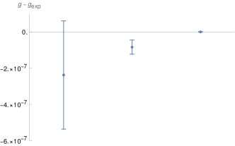
    theo, prev           theo,new           exp

Figure 4: Previous and updated theoretical values of the bound-electron $g$-factor in ¹¹⁸Sn⁴⁹⁺, compared with the experimental $g$-factor value from Ref. Morgner et al. (2023).

Summary – We completed the calculation of the two-loop self-energy corrections to the bound-electron $g$-factor in hydrogenlike ions. The completed SESE theory allows us to significantly improve the overall theoretical accuracy of the bound-electron $g$-factor in the medium- to high-$Z$ regime. Our improved result also enables a more detailed test of virtual light-by-light scattering contributions Morgner et al. (2023). We demonstrated this by presenting an updated theoretical $g$-factor of hydrogenlike tin whose uncertainty is improved by almost one order-of-magnitude compared to the previous best theory and which is now significantly limited by nuclear effects. For even higher $Z>50$, uncertainties due to nuclear effects are expected to be significantly larger, while the uncertainty of the SESE effect can be expected to be comparable to this work. This paves the way to a $g$-factor theory which will be primarily limited by nuclear effects, or, in turn, can be applied to extract nuclear root-mean-square radii from experimental $g$-factors and to improved searches towards new physics effects Debierre et al. (2020); Sailer et al. (2022).

We thank N. Oreshkina, H. Cakir and J. Morgner for insightful discussions. Supported by the Deutsche Forschungsgemeinschaft (DFG, German Research Foundation) Project-ID 273811115 - SFB 1225.

References

- Fan et al. (2023) X. Fan, T. G. Myers, B. A. D. Sukra, and G. Gabrielse, Phys. Rev. Lett. 130, 071801 (2023).
- Laporta and Remiddi (1996) S. Laporta and E. Remiddi, Phys. Lett. B 379, 283 (1996).
- Laporta (2017) S. Laporta, Phys. Lett. B 772, 232 (2017).
- Aoyama et al. (2012) T. Aoyama, M. Hayakawa, T. Kinoshita, and M. Nio, Phys. Rev. Lett. 109, 111807 (2012).
- Volkov (2019) S. Volkov, Phys. Rev. D 100, 096004 (2019).
- Karshenboim (2000) S. G. Karshenboim, Phys. Lett. A 266, 380 (2000).
- Czarnecki et al. (2000) A. Czarnecki, K. Melnikov, and A. Yelkhovsky, Phys. Rev. A 63, 012509 (2000).
- Pachucki et al. (2005) K. Pachucki, A. Czarnecki, U. D. Jentschura, and V. A. Yerokhin, Phys. Rev. A 72, 022108 (2005).
- Czarnecki et al. (2018) A. Czarnecki, M. Dowling, J. Piclum, and R. Szafron, Phys. Rev. Lett. 120, 043203 (2018).
- Yerokhin et al. (2004) V. A. Yerokhin, P. Indelicato, and V. M. Shabaev, Phys. Rev. A 69, 052503 (2004).
- Karshenboim et al. (2001) S. G. Karshenboim, V. G. Ivanov, and V. M. Shabaev, J. Exp. Theor. Phys. Lett. 93, 477 (2001).
- Beier (2000) T. Beier, Phys. Rep. 339, 79 (2000).
- Sturm et al. (2011) S. Sturm, A. Wagner, B. Schabinger, J. Zatorski, Z. Harman, W. Quint, G. Werth, C. H. Keitel, and K. Blaum, Phys. Rev. Lett. 107, 023002 (2011).
- Sturm et al. (2013) S. Sturm, A. Wagner, M. Kretzschmar, W. Quint, G. Werth, and K. Blaum, Phys. Rev. A 87, 030501(R) (2013).
- Köhler et al. (2016) F. Köhler, K. Blaum, M. Block, S. Chenmarev, S. Eliseev, D. A. Glazov, M. Goncharov, J. Hou, A. Kracke, D. A. Nesterenko, et al., Nat. Commun. 7, 10246 (2016).
- Arapoglou et al. (2019) I. Arapoglou, A. Egl, M. Höcker, T. Sailer, B. Tu, A. Weigel, R. Wolf, H. Cakir, V. A. Yerokhin, N. S. Oreshkina, et al., Phys. Rev. Lett. 122, 253001 (2019).
- Sturm et al. (2014) S. Sturm, F. Köhler, J. Zatorski, A. Wagner, Z. Harman, G. Werth, W. Quint, C. H. Keitel, and K. Blaum, Nature 506, 467 (2014).
- Köhler et al. (2015) F. Köhler, S. Sturm, A. Kracke, G. Werth, W. Quint, and K. Blaum, Journal of Physics B: Atomic, Molecular and Optical Physics 48, 144032 (2015).
- Zatorski et al. (2017) J. Zatorski, B. Sikora, S. G. Karshenboim, S. Sturm, F. Köhler-Langes, K. Blaum, C. H. Keitel, and Z. Harman, Phys. Rev. A 96, 012502 (2017).
- Shabaev et al. (2006) V. M. Shabaev, D. A. Glazov, N. S. Oreshkina, A. V. Volotka, G. Plunien, H.-J. Kluge, and W. Quint, Phys. Rev. Lett. 96, 253002 (2006).
- Yerokhin et al. (2016) V. A. Yerokhin, E. Berseneva, Z. Harman, I. I. Tupitsyn, and C. H. Keitel, Phys. Rev. Lett. 116, 100801 (2016).
- Cakir et al. (2020) H. Cakir, N. S. Oreshkina, I. A. Valuev, V. Debierre, V. A. Yerokhin, C. H. Keitel, and Z. Harman, ArXiv Atomic Physics (2020), arXiv:2006.14261v1 [physics.atom-ph].
- Debierre et al. (2020) V. Debierre, C. Keitel, and Z. Harman, Physics Letters B 807, 135527 (2020).
- Sailer et al. (2022) T. Sailer, V. Debierre, Z. Harman, F. Heiße, C. König, J. Morgner, B. Tu, A. V. Volotka, C. H. Keitel, K. Blaum, et al., Nature 606, 479 (2022).
- Schneider et al. (2022) A. Schneider, B. Sikora, S. Dickopf, M. Müller, N. S. Oreshkina, A. Rischka, I. A. Valuev, S. Ulmer, J. Walz, Z. Harman, et al., Nature 606, 878 (2022).
- Dickopf et al. (2024) S. Dickopf, B. Sikora, A. Kaiser, M. Müller, S. Ulmer, V. A. Yerokhin, Z. Harman, C. H. Keitel, A. Mooser, and K. Blaum, Nature (2024).
- Heiße et al. (2023) F. Heiße, M. Door, T. Sailer, P. Filianin, J. Herkenhoff, C. M. König, K. Kromer, D. Lange, J. Morgner, A. Rischka, et al., Phys. Rev. Lett. 131, 253002 (2023).
- Morgner et al. (2023) J. Morgner, B. Tu, C. M. König, T. Sailer, F. Heiße, H. Bekker, B. Sikora, C. Lyu, V. A. Yerokhin, Z. Harman, et al., Nature 622, 53 (2023).
- Sturm et al. (2019) S. Sturm, I. Arapoglou, A. Egl, M. Höcker, S. Kraemer, T. Sailer, B. Tu, A. Weigel, R. Wolf, J. C. López-Urrutia, et al., The European Physical Journal Special Topics 227, 1425 (2019).
- Herfurth et al. (2015) F. Herfurth, Z. Andelkovic, W. Barth, W. Chen, L. A. Dahl, S. Fedotova, P. Gerhard, M. Kaiser, O. K. Kester, H.-J. Kluge, et al., Physica Scripta 2015, 014065 (2015).
- Yerokhin and Harman (2013) V. A. Yerokhin and Z. Harman, Phys. Rev. A 88, 042502 (2013).
- Debierre et al. (2021) V. Debierre, B. Sikora, H. Cakir, N. S. Oreshkina, V. A. Yerokhin, C. H. Keitel, and Z. Harman, Phys. Rev. A 103, L030802 (2021).
- Mallampalli and Sapirstein (1998) S. Mallampalli and J. Sapirstein, Phys. Rev. A 57, 1548 (1998).
- Shabaev (2003) V. M. Shabaev, in Precision Physics of Simple Atomic Systems, edited by S. G. Karshenboim and V. B. Smirnov (Springer-Verlag, Berlin Heidelberg, 2003), pp. 97–113.
- Yerokhin et al. (2003) V. A. Yerokhin, P. Indelicato, and V. M. Shabaev, Eur. Phys. J. D 25, 203 (2003).
- Sikora et al. (2020) B. Sikora, V. A. Yerokhin, N. S. Oreshkina, H. Cakir, C. H. Keitel, and Z. Harman, Phys. Rev. Research 2, 012002(R) (2020).
- Breit (1928) G. Breit, Nature 122, 649 (1928).
- Sikora (2018) B. Sikora, Ph.D. thesis, University of Heidelberg (2018).
- Peskin and Schroeder (1995) M. E. Peskin and D. V. Schroeder, An Introduction to Quantum Field Theory (Westview Press, 1995).
- Yerokhin (2018) V. A. Yerokhin, Phys. Rev. A 97, 052509 (2018).
- Yerokhin and Maiorova (2020) V. A. Yerokhin and A. V. Maiorova, Symmetry 12 (2020).
- Yerokhin (2010) V. A. Yerokhin, Eur. Phys. J. D 58, 57 (2010).
- Mohr and Taylor (2000) P. J. Mohr and B. N. Taylor, Rev. Mod. Phys. 72, 351 (2000).
- Shabaev (2002) V. M. Shabaev, Phys. Rep. 356, 119 (2002).
- Holmberg et al. (2015) J. Holmberg, A. N. Artemyev, A. Surzhykov, V. A. Yerokhin, and T. Stöhlker, Phys. Rev. A 92, 042510 (2015).
- Yerokhin et al. (2005) V. A. Yerokhin, K. Pachucki, and V. M. Shabaev, Phys. Rev. A 72, 042502 (2005).
- Petermann (1957) A. Petermann, Helv. Phys. Acta 30, 407 (1957).
- Sommerfield (1958) C. M. Sommerfield, Ann. Phys. 5, 26 (1958).