Hausdorff dimension, diverging Schottky representations and the infinite dimensional hyperbolic space

Abstract

One of our main goals in this paper is to understand the behavior of limit sets of a diverging sequence of Schottky groups in $\operatorname{Isom}\,\mathbf{H}^{N}$. This leads us to a generalization of a classical theorem of Bowen on variations of Hausdorff dimension of limit sets; and to a method of transforming a diverging sequence of Schottky groups in $\operatorname{Isom}\,\mathbf{H}^{N}$ into an almost converging sequence in $\operatorname{Isom}\,\mathbf{H}^{\infty}$. Our results apply in particular to an example of McMullen and generalize a previous work by Mehmeti and Dang.

1 Introduction

One of our main goals in this paper is to understand the behavior of limit sets of a diverging sequence of Schottky groups in $\operatorname{Isom}\,\mathbf{H}^{N}$.

Schottky groups are generated by a finite set of hyperbolic isometries $S=\{s_{1},...,s_{r}\}$, $2\leq r$, of $\operatorname{Isom}\,\mathbf{H}^{N}$ such that there exists open subsets with disjoint closure $(D_{i}^{\pm})_{1\leq i\leq r}$ in $\mathbf{H}^{N}\cup\partial\mathbf{H}^{N}$ satisfying

$$s_{i}^{\pm}(D_{i}^{\pm})\subset D_{i}^{\mp}.$$ (1)

By the classical ’ping-pong’ argument, such a group is discrete and free. It may be then considered as the image $\rho(\mathbf{F}_{r})$ of the free group on $r$ generators by a discrete and faithful representation $\rho:\mathbf{F}_{r}\rightarrow\operatorname{Isom}\,\mathbf{H}^{N}$.

In this paper, the space of representations of a finitely generated group $\Gamma$ into the isometry group $\operatorname{Isom}\,X$ of a metric space is denoted by

$$\operatorname{Rep}_{X}(\Gamma).$$

Moreover, we denote by $\operatorname{Rep}^{\mathrm{Schottky}}_{\mathbf{H}^{N}}(\mathbf{F}_{r})$ the subspace of $\operatorname{Rep}_{\mathbf{H}^{N}}(\Gamma)$ such that $\rho(\mathbf{F}_{r})$ is a Schottky group. For any $\rho$ in $\operatorname{Rep}^{\mathrm{Schottky}}_{\mathbf{H}^{N}}(\mathbf{F}_{r})$, we denote by $\Lambda_{\rho}$ the limit set of $\rho(\mathbf{F}_{r})$. The Hausdorff dimension $\operatorname{Hdim}\Lambda_{\rho}$ of a subset $\Lambda\subset\partial\mathbf{H}^{N}$ is computed with respect to the visual distance at a base point $o\in\mathbf{H}^{N}$ on $\partial\mathbf{H}^{N}$, see Section 2.2.

The variations of the limit set $\Lambda_{\rho}$ and its Hausdorff dimension $\operatorname{Hdim}\Lambda_{\rho}$ ,when $\rho$ varies in $\operatorname{Rep}^{\mathrm{Schottky}}_{\mathbf{H}^{N}}(\mathbf{F}_{r})$, has been studied thoroughly. The following celebrated continuity result is a consequence of the work of Bowen [Bow79].

Theorem 1.1 ([Bow79]).

Let $\rho_{k}$, $k\in\mathbf{N}$, and $\rho$ be Schottky representations in the space $\operatorname{Rep}^{\mathrm{Schottky}}_{\mathbf{H}^{N}}(\mathbf{F}_{r})$. We assume that $\lim_{k}\rho_{k}(g)=\rho(g)$ for every $g\in\mathbf{F}_{r}$. Then,

$$\lim_{k}\operatorname{Hdim}\Lambda_{\rho_{k}}=\operatorname{Hdim}\Lambda_{\rho}.$$

One motivating question for this paper is the following: what happens when the sequence $\rho_{k}$ is diverging? In the sequel, we study the asymptotic behavior of $\operatorname{Hdim}\Lambda_{\rho_{k}}$ in the general situation where $\rho_{k}\in\operatorname{Rep}^{\mathrm{Schottky}}_{\mathbf{H}^{N}}(\mathbf{F}_{r})$ diverges, i.e. the minimal joint displacement $r_{k}$ of the generators goes to $+\infty$ (see Section 4.2.2 for a precise definition), where:

$$r_{k}:=\inf_{x\in\mathbf{H}^{N}}\max_{1\leq j\leq r}d(x,\rho_{k}(s_{j})x).$$

In this case, we expect that each Schottky set $D_{i}^{\pm}$ as defined in (1) tends to a point and that the Hausdorff dimension $\operatorname{Hdim}\Lambda_{\rho_{k}}$ tends to $0$. We want to give an asymptotic expansion for the sequence.

This question will lead us to a generalization of Bowen Theorem 1.1, see Theorem 1.7; and to a method of transforming a diverging sequence of Schottky groups in $\operatorname{Isom}\,\mathbf{H}^{N}$ into an almost converging sequence in $\operatorname{Isom}\,\mathbf{H}^{\infty}$, see Theorem 1.10.

1.1 Revisiting an example of McMullen

Our results apply in particular to an example of McMullen, that can be used as a guideline to our paper. This example indeed describes such an asymptotic.

Example 1.2 (McMullen example).

In [McM98], C. McMullen studies the family of discrete groups $G_{\theta}<\operatorname{Isom}\,\mathbf{H}^{2}$ generated by three reflections $\sigma_{1}$, $\sigma_{2}$ and $\sigma_{3}$ in three disjoint symmetric circles, each orthogonal to $\partial\mathbf{H}^{2}$ in an arc of length $0<\theta<2\pi/3$. The index $2$ subgroup $\Gamma_{\theta}<G_{\theta}$ of orientation preserving isometries of $G_{\theta}$ is a Schottky group on two generators $\rho_{\theta}(s_{1}):=\sigma_{1}\,\sigma_{2}$ and $\rho_{\theta}(s_{2}):=\sigma_{1}\,\sigma_{3}$. When $\theta$ goes to $0$, the family of representations $\rho_{\theta}$ of the free group on two generators such that $\rho_{\theta}(\mathbf{F}_{2})=\Gamma_{\theta}$ is diverging and McMullen shows that

$$\operatorname{Hdim}\Lambda_{\rho_{\theta}}\sim\frac{\log 2}{2|\log\theta|}.$$ (2)

Drawing a parallel with Theorem 1.1, we need a limiting representation to describe the asymptotic. A classical construction due to Morgan-Shalen [MS84], through an ultrafilter, renormalization and asymptotic cones, see Section 4.2.2, gives that the sequence $(\mathbf{H}^{N},r_{k}^{-1}d)$ converges to an action of $\mathbf{F}_{r}$ on a minimal tree $(T,d_{T})$ in the equivariant Gromov-Hausdorff topology. We denote by $\rho_{\infty}:\mathbf{F}_{r}\to\operatorname{Isom}\,T$ the associated representation.

Let us assume, as in Theorem 1.1 for converging sequences, that the limiting representation $\rho_{\infty}$ is a Schottky representation, with the same definition as for representations into $\operatorname{Isom}\,\mathbf{H}^{n}$ and the disc $D_{i}$’s being inside $\partial T$. Let $\Lambda_{\infty}$ be the limit set of $\rho_{\infty}(\mathbf{F}_{r})\subset\partial T$. The tree is a $\operatorname{CAT}(-1)$-metric space and its boundary $\partial T$ may naturally be equipped with a visual distance $d_{p}$ (for a given base-point $p\in T$), see Section 2.2. For a subset $\Lambda\subset\partial T$, we still denote by $\operatorname{Hdim}\Lambda$ the Hausdorff dimension of $\Lambda$ with respect to the distance $d_{p}$. The following Theorem is one of the main result in this paper and explains the asymptotic expansion in McMullen example:

Theorem 1.3.

Let $(\rho_{k})_{k\in\mathbf{N}}$ be a sequence of diverging representations in the space $\operatorname{Rep}_{\mathbf{H}^{N}}(\mathbf{F}_{r})$ with joint displacement $r_{k}$. Assume that the limit action of $\rho_{\infty}(\mathbf{F}_{\nu})$ on the minimal tree $T$ is Schottky. Then, up to a subsequence,

$$\lim_{k}\;r_{k}\cdot\operatorname{Hdim}\Lambda_{\rho_{k}}=\operatorname{Hdim}\Lambda_{\rho_{\infty}}.$$

Remark 1.4.

We will give two different interpretations of the expression up to a subsequence. Indeed, as already briefly mentioned, the actual construction of $\rho_{\infty}$ depends on a choice of an ultrafilter $\omega$, see Section 4.2. We will prove first that $\operatorname{Hdim}\Lambda_{\rho_{\infty}}$ is the $\omega$-limit of $r_{k}\cdot\operatorname{Hdim}\Lambda_{\rho_{k}}$, see Theorem 5.8. But, then, in Proposition 5.9, we will explain how to construct an actual subsequence with convergence. Still, this subsequence is not very natural because we cannot guarantee that its set of indices belongs to the ultrafilter $\omega$, see Section 5.5.

Remark 1.5.

The question of the asymptotic expansion for Hausdorff dimension of limit sets of diverging Schottky groups has already been studied. In particular, the previous Theorem 1.3 has been proved by V. Mehmeti and N.B. Dang in the case $N=2,3$, [DM24], under a slightly more stringent assumption on $\rho_{\infty}$. The proof, though in several points close to ours, goes through the theory of analytic spaces of Berkovich to deal with the convergence, where we will mostly use non locally compact $\operatorname{CAT}(-1)$-spaces, such as the (unique up to isometry) separable infinite dimensional hyperbolic space $\mathbf{H}^{\infty}$, see Section 2.1.

Let us now come back to McMullen example:

Example 1.6 (McMullen example, continued).

In the above example $\rho_{\theta}$ of McMullen, we can compute that the joint displacement of $\rho_{\theta}$ verifies:

$$r_{\theta}\sim 4|\log(\theta/2)|.$$

Notice that the limit group $\rho_{\infty}(\mathbf{F}_{2})$ acts on a trivalent tree $T$ with quotient a graph with two vertices joined by three edges $\alpha,\beta,\gamma$ of length $1/2$ where the loops $\gamma.\alpha$ and $\gamma.\beta$ generate $\rho_{\infty}(\mathbf{F}_{2})$, see Figure 1.

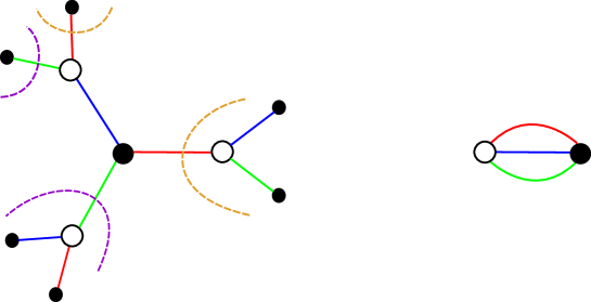
Figure 1: McMullen example: Schottky action of $\rho_{\infty}$ on its minimal tree (left); quotient of this action (right).

Therefore, the limit set of $\rho_{\infty}(\mathbf{F}_{2})$ coincides with $\partial T$ and its Hausdorff dimension satisfies $\operatorname{Hdim}\Lambda_{\rho_{\infty}}=2\log 2$. Theorem 1.3, or more precisely its version Proposition 5.9, states that (see Example 5.10):

$$\lim_{\theta\to 0}r_{\theta}\operatorname{Hdim}\Lambda_{\rho_{\theta}}=\lim_{\theta\to 0}4|\log(\theta/2)|\operatorname{Hdim}\Lambda_{\rho_{\theta\to 0}}=\operatorname{Hdim}\Lambda_{\rho_{\infty}}=2\log 2$$

and we recover the estimate (2) of McMullen: $\operatorname{Hdim}\Lambda_{\rho_{\theta}}\sim_{\theta\to 0}\frac{\log 2}{2|\log\theta|}$.

We prove Theorem 1.3 following closely Bowen’s method, see Section 3. The main obstacle for doing so is that the limit sets $\Lambda_{\infty}$ and $\Lambda_{k}$’s do not live in the same space, which seems to rule out all approximation arguments needed. So our strategy has two steps, which are mainly independent and have each their own interest:

1. The first step is to actually transform the Gromov-Hausdorff convergence of $\rho_{k}$ to $\rho_{\infty}$ into a weak kind of convergence of a sequence $R_{k}:\mathbf{F}_{r}\to\operatorname{Isom}\,\mathbf{H}^{\infty}$ to $R_{\infty}:\mathbf{F}_{r}\to\operatorname{Isom}\,\mathbf{H}^{\infty}$, see Section 1.3 below for more details. Moreover, still denoting by $r_{k}$ the joint displacement of $\rho_{k}$, we will have the following formula for the Hausdorff dimensions of limit sets:

   $$r_{k}\operatorname{Hdim}\Lambda_{k}=\operatorname{Hdim}\Lambda_{R_{k}}\quad\textrm{and}\quad\operatorname{Hdim}\Lambda_{\infty}=\operatorname{Hdim}\Lambda_{R_{\infty}}$$ (3)

   Beware that in these equations, the $\Lambda_{k}$’s are inside $\partial\mathbf{H}^{N}$, $\Lambda_{\infty}$ inside $\partial T$ and all the $\Lambda_{R_{k}}$ inside $\partial\mathbf{H}^{\infty}$.

2. The second step is to state and prove a general version of Bowen that encompass our weak type of convergence. It is best stated in the realm of non locally compact $\operatorname{CAT}(-1)$-spaces, see Section 1.2. It implies the convergence, up to a subsequence:

   $$\operatorname{Hdim}\Lambda_{R_{k}}\to\operatorname{Hdim}\Lambda_{R_{\infty}}.$$ (4)

Eqs. (3) and (4) together give Theorem 1.3, see Section 5.4 for more details. We now describe more thoroughly those two steps. We choose to begin with the second step, to reflect the structure of our paper.

1.2 Bowen Theorem for non locally compact $\operatorname{CAT}(-1)$-spaces

Section 3 of this paper will be devoted to prove the extension of Bowen’s Theorem. We will work in the quite general setting of complete $\operatorname{CAT}(-1)$-spaces without assuming local compactness. One example of such a space is the infinite dimensional separable hyperbolic space $\mathbf{H}^{\infty}$, see Example 2.2. Needed facts about $\operatorname{CAT}(-1)$-geometry are reviewed in Section 2. Matters of convergence, discreteness, convex-cocompactness and related topics for the isometry group of such a space can be delicate [DSU17, Duc23, Xu24]. A non trivial notion is the one of Schottky representations. We define it in Definition 3.1 as quasi-isometric representations of $\mathbf{F}_{r}$ to $\operatorname{Isom}\,X$, i.e. representations $\rho$ such that the orbit map $\tau_{\rho}:\mathbf{F}_{r}\to X$, defined by $\tau_{\rho}(g)=\rho(g)\cdot o$ for all $g\in\mathbf{F}_{r}$, is a quasi isometric embedding of the (vertices of the) Cayley graph of $\mathbf{F}_{r}$ to $X$. The space of such representations is denoted by $\operatorname{Rep}_{X}^{\mathrm{Schottky}}(\mathbf{F}_{r})$. We prove the following, without assuming $X$ to be locally compact.

Theorem 1.7 (Bowen theorem for $\operatorname{CAT}(-1)$-spaces).

Let $(X,d,o)$ be a complete pointed $\operatorname{CAT}(-1)$-space; consider a sequence $(R_{k})_{k\in\mathbf{N}}$ in $\operatorname{Rep}_{X}(\mathbf{F}_{r})$ and $R_{\infty}\in\operatorname{Rep}_{X}^{\mathrm{Schottky}}(\mathbf{F}_{r})$ a Schottky representation. Assume that the sequence of orbit maps $(\tau_{k})_{k\in\mathbf{N}}$ converges point-wise to $\tau_{\infty}$:

$$\forall g\in\mathbf{F}_{r},\quad\tau_{k}(g)=R_{k}(g)\cdot o\xrightarrow{k\to\infty}\tau_{\infty}(g)=R_{\infty}(g)\cdot o.$$

Then we have:

1. The sequence of limit sets $(\Lambda_{k})_{k\in\mathbf{N}}$ of $(R_{k})_{k\in\mathbf{N}}$ converges, in the Hausdorff topology of $\partial X$, to the limit set $\Lambda_{\infty}$ of $R_{\infty}$.

2. The sequence $\operatorname{Hdim}\Lambda_{k}$ converges to $\operatorname{Hdim}\Lambda_{\infty}$.

The assumption in the previous Theorem is a consequence of the convergence of $R_{k}$ to $R_{\infty}$ in $\operatorname{Rep}_{X}(\Gamma)$ (see Section 2 for precisions on the compact-open topology of this set). This leads to the following Corollary; it is not surprising, but has not been stated to the best of our knowledge:

Corollary 1.8.

Let $X$ be a complete $\operatorname{CAT}(-1)$-space, consider $(R_{k})_{k\in\mathbf{N}}$ a sequence of representations in $\operatorname{Rep}_{X}(\mathbf{F}_{r})$ and $R_{\infty}$ in $\operatorname{Rep}_{X}^{\mathrm{Schottky}}(\mathbf{F}_{r})$. Assume that $\lim_{k}R_{k}(g)=R_{\infty}(g)$ for every $g\in\mathbf{F}_{r}$. Then,

$$\lim_{k}\operatorname{Hdim}(\Lambda_{R_{k}})=\operatorname{Hdim}(\Lambda_{R_{\infty}}).$$

We now present more precisely the construction of the representations $R_{k}$ a,d $R_{\infty}$.

1.3 Turning diverging sequences of representations into convergent ones

We work here with a finitely generated $\Gamma$, not especially a free group. When considering diverging sequences of representations of $\Gamma$ into $\operatorname{Isom}\,\mathbf{H}^{N}$, it has become classical to consider asymptotic cones of sequences of rescaled hyperbolic spaces $X_{k}=(\mathbf{H}^{N},r_{k}^{-1}d_{\mathbf{H}^{N}},o_{k})$, where $r_{k}$ is a sequence of positive real numbers tending to infinity and $o_{k}\in\mathbf{H}^{N}$. Paulin [Pau97], see also [Bes88], has explained how the sequence of pointed metric spaces $X_{k}$ converges in the equivariant Gromov-Hausdorff topology to its asymptotic cone, denoted by $X_{\omega}$.

However, this type of convergence does not allow to apply Theorem 1.7. In Section 5, we examine how to promote this equivariant Gromov-Hausdorff convergence to one in the realm of the Theorem. When looking for a better type of convergence, one could hope to get an actual Hausdorff convergence as subsets of a fixed metric space: is it possible to embed isometrically and equivariantly each $X_{k}$ and $X_{\omega}$ in a metric space $Y$ such that $X_{k}$ goes to $X_{\omega}$ in the Hausdorff topology of subsets of $Y$? It is indeed the case for compact spaces, cf [BBI01, Section 7.3]

Note that $X_{\omega}$ is not locally compact, so this would imply that $Y$ is not locally compact either. Natural candidates for $Y$ are, as such, infinite dimensional hyperbolic spaces. Indeed, nice equivariant embeddings of hyperbolic spaces [MP14, MP19] and trees [DSU17, MP19] into infinite dimensional hyperbolic spaces have been defined and studied. We will use these embeddings. However, the answer to this crude question is no!

Proposition 1.9.

There is no metric space $Y$, and sequences of isometric embeddings $f_{k}:X_{k}\to Y$ and $f:X_{\omega}\to Y$ such that:

• The limit of any sequence $f_{k}(x_{k})$ equals the image by $f$ of the point $[(x_{i})]$ in $X_{\omega}$;

• $f_{i}(X_{i})$ converges, in the Hausdorff topology of $Y$, to $f(X_{\omega})$.

Proof.

Indeed, one can look at the unit spheres in $X_{k}$ and $X_{\omega}$: the fact that $X_{\omega}$ is a complete real tree implies that, for any $0<\epsilon<2$, any ball of radius $\epsilon$ in the unit sphere is its own $\epsilon$-neighborhood.

On the contrary, in any $X_{k}$, the sphere is $\epsilon$-connected: for any pair of points, there is a chain of points connecting them, with each steps of length $<\epsilon$.

This contradicts Hausdorff convergence of $f_{k}(X_{k})$ to $f(X_{\omega})$ in $Y$: the limit of a sequence of $\epsilon$-connected subsets should be included in a single ball of radius $\epsilon$ in the image of the unit sphere in $f(X_{\omega})$ ∎

So we are looking for an intermediate notion of convergence. In order to explain it, let us come back to [MP19]. Monod and Py studied the self-representations of the infinite dimensional Möbius group, based on the notion of kernel of hyperbolic type introduced by Gromov. They have in particular shown, building on their previous [MP14] and other contributions [BIM05, DSU17], that there are:

• a one-parameter family of continuous embeddings $f_{t}:\mathbf{H}^{N}\rightarrow\mathbf{H}^{\infty}$, for all $0\leq t\leq 1$, which are equivariant for a family of representations $\nu_{t}:\operatorname{Isom}\,\mathbf{H}^{N}\to\operatorname{Isom}\,\mathbf{H}^{\infty}$. Denoting by $d$ both the distance in $\mathbf{H}^{N}$ and $\mathbf{H}^{\infty}$, they verify for all $x,y\in\mathbf{H}^{N}$:

  $$(\cosh{d(x,y)})^{t}=\cosh{d(f_{t}(x),f_{t}(y))}$$

  They are very close to being simple dilatations by a factor $t$ and are anyway $1$-Lipschitz, see Proposition 4.5. They naturally extend to embeddings of $\partial\mathbf{H}^{N}$ to $\partial\mathbf{H}^{\infty}$. The functions $f_{t}$ are well-defined up to post-composition by an isometry of $\mathbf{H}^{\infty}$ as well as the representations $\nu_{t}$ up to conjugation by the same isometry. We fix one such choice.

• for any separable tree $T$, a one-parameter family of continuous embeddings $F_{s}:T\rightarrow\mathbf{H}^{\infty}$, for all $0\leq s$, which are equivariant for a family of representations $\mu_{s}:\operatorname{Isom}\,T\to\operatorname{Isom}\,\mathbf{H}^{\infty}$. They are very close to being simple dilatations by a factor $s$. Here also, the functions $F_{s}$ and representations $\mu_{s}$ are well-defined, up to an isometry of $\mathbf{H}^{\infty}$ and we fix one choice.

Those constructions are briefly reviewed in Section 4.1.

With these families, we can explain our manipulation on the representations $\rho_{k}$, with joint displacement $r_{k}$, and $\rho_{\infty}$. Indeed, let $\rho_{k}$ be a diverging sequence of representations, $T$ be the minimal invariant tree in the asymptotic cone, which is separable, and $\rho_{\infty}$ be the limiting representation. Define $R_{\infty}$ to be the composition $\mu_{1}\circ\rho_{\infty}$. It acts on $F_{1}(T)$ which is an almost isometric embedding of $T$ in $\mathbf{H}^{\infty}$. In particular, $F_{1}$ defines a Lipschitz embedding of $\partial T$ to $\partial\mathbf{H}^{\infty}$.

The asymptotic cone $X_{\omega}$ and the minimal tree $T$ are obtained by renormalizing the metric space $\mathbf{H}^{N}$ by the factor $r_{k}^{-1}$. The main observation of our paper is that this renormalization can be actually almost isometrically embedded into $\mathbf{H}^{\infty}$, by considering $f_{r_{k}^{-1}}(\mathbf{H}^{N})$, for all $k$ such that $r_{k}>1$. It is not hard to see that the sequence of actions of $\Gamma$ on $f_{r_{k}^{-1}}(\mathbf{H}^{N})\subset\mathbf{H}^{\infty}$, through $\nu_{r_{k}^{-1}}\circ\rho_{k}$, converges in the equivariant Gromov-Hausdorff sense to the action of $\Gamma$ on $F_{1}(T)\subset\mathbf{H}^{\infty}$, through $R_{\infty}$. The content of our third Theorem is that we can choose a sequence $\mathcal{I}_{k}$ of isometries of $\mathbf{H}^{\infty}$, defining the representations and the $R_{k}$-equivariant embeddings $\phi_{k}$ by:

$$R_{k}:=\mathcal{I}_{k}\circ(\nu_{r_{k}^{-1}}\circ\rho_{k})\circ\mathcal{I}_{k}\textrm{ and }\phi_{k}:=\mathcal{I}_{k}\circ f_{r_{k}^{-1}}:\mathbf{H}^{N}\to\mathbf{H}^{\infty}\textrm{ with }\phi_{k}\circ\rho_{k}=R_{k}\circ\phi_{k},$$

such that the convergence of $\phi_{k}(X_{k})$ to $F_{1}(T)$ is much better and close to an actual Hausdorff convergence. We call this new convergence a partial equivariant Hausdorff convergence. Its actual definition needs the choice of an ultrafilter; informally, equivariant partial Hausdorff convergence is defined in the following way (see Definition 5.1):

We say that a sequence of embeddings $(\phi_{k})_{k\in\mathbf{N}}:\mathbf{H}^{N}\to\mathbf{H}^{\infty}$ realizes a partial equivariant Hausdorff convergence of $\mathbf{H}^{N}$ to $F_{1}(T)$ if one can construct a sequence of finite subsets $(K_{k})_{k\in\mathbf{N}}$ of $\mathbf{H}^{N}$ such that $F_{1}(T)$ is the set of accumulation points of sequences $(\phi_{k}(x_{k}))$, where $x_{k}\in K_{k}$ and the actions of $\Gamma$ on $F_{1}(T)$ through $R_{\infty}$ and on sequences through the sequence $(R_{k})$ are compatible.

Our third main Theorem completes the first step of the strategy for Theorem 1.3:

Theorem 1.10 (Equivariant partial Hausdorff convergence, see Theorem 5.2).

For any diverging sequence $\rho_{k}:\Gamma\to\operatorname{Isom}\,\mathbf{H}^{N}$, with the notations above, one can choose a sequence $\mathcal{I}_{k}$ of isometries of $\mathbf{H}^{\infty}$ such that the sequence of embeddings $(\phi_{k}:=\mathcal{I}_{k}\circ f_{r_{k}^{-1}})_{k\in\mathbf{N}}$ realizes a partial equivariant Hausdorff convergence of $\mathbf{H}^{N}$ to $F_{1}(T)$.

Moreover, the representations $R_{k}$ preserve $\mathcal{I}_{k}(\mathbf{H}^{N})$ and the sequence of orbit maps $(\tau_{R_{k}})_{k\in\mathbf{N}}$ "converges" point-wise to $\tau_{R_{\infty}}$.

Above, the notion of "convergence" is actually a convergence along the ultrafilter, see Theorem 5.2 for the precise statement. Surprisingly, a variation of our theorem is given in Section 5.5, where explicit subsequences are build along which the representations $R_{k}$ actually converge toward $R_{\infty}$ in $\operatorname{Rep}_{\mathbf{H}^{\infty}}(\Gamma)$. In particular, it shows that our construction for McMullen example leads to an actual convergence of $R_{\theta}$ to $R_{\infty}$ in $\operatorname{Rep}_{\mathbf{H}^{\infty}}(\Gamma)$, see Example 5.10.

The conclusion of Theorem 1.10 is what we need to apply our Theorem 1.7 to the sequence $R_{k}$. As, moreover, $\phi_{k}:=\mathcal{I}_{k}\circ f_{r_{k}^{-1}}$ is almost homothetic by a factor $r_{k}^{-1}$, the induced map between limit sets $\Lambda_{\rho_{k}}$ and $\Lambda_{R_{k}}:=\phi_{k}(\Lambda_{\rho_{k}})$ acts as an exponentiation to the power $r_{k}^{-1}$ on the visual distances, see Section 5.4. Hence the Hausdorff dimensions verify Eq. (3):

$$r_{k}\operatorname{Hdim}\Lambda_{\rho_{k}}=\operatorname{Hdim}\Lambda_{R_{k}}.$$

This proves Theorem 1.3 and concludes the paper.

1.4 Acknowledgments

The authors express their deep gratitude to Nguyen-Bac Dang, Vlerë Mehmeti, Frédéric Naud, Anne Parreau, Frédéric Paulin, Pierre Py, Samuel Tapie, Teddy Weisman, Pierre Will, David Xu and more generally all the members of ANR-23-CE40-0012-03 project HilbertXField for fruitful discussions and their enlightning comments.

Contents

1. 1 Introduction
2. 2 CAT(-1)-geometry
3. 3 Convergence of Hausdorff dimensions for Schottky actions in CAT(-1)-spaces
4. 4 Kernels, embeddings and asymptotic cones
5. 5 Partial Hausdorff convergence of embeddings

2 CAT(-1)-geometry

We review in this section standard notations and known facts about $\operatorname{CAT}(-1)$-geometry and prove a few results we will need later on. For convenience, our main reference will be [DSU17]; see also [BH99]. The main examples to keep in mind are $\mathbf{H}^{\infty}$, metric trees and more generally what [DSU17] calls a ROSSONCT.

2.1 $\operatorname{CAT}(-1)$-spaces

A $\operatorname{CAT}(-1)$-space $(X,d)$ is a geodesic metric space which satisfy the $\operatorname{CAT}(-1)$-inequality [DSU17, Eq. (3.2.1)] expressing that triangles are thinner than in the hyperbolic plane. We will always assume our $\operatorname{CAT}(-1)$-space to be complete, but not necessarily to be locally compact (or proper). Such a space admits an ideal boundary $\partial X$, see [DSU17, Section 3.4]. We will not precisely define it here, but still define two important functions on a $\operatorname{CAT}(-1)$-space: Gromov product and Busemann functions.

Definition 2.1.

Let $X$ be a $\operatorname{CAT}(-1)$-space, for three points $x,y,z$ in $X$, the Gromov product of $x$ and $y$ w.r.t. $z$ is:

$$\langle x,y\rangle_{z}:=\frac{1}{2}\left(d(x,z)+d(y,z)-d(x,y)\right);$$

the Busemann function is: $x,y,z\mapsto B(x,y,z)=d(x,z)-d(y,z)$.

Note that [DSU17] denotes this last function by $B_{z}(x,y)$. Those functions are invariant under the action of $\operatorname{Isom}\,X$ on all variables simultaneously. In the language of hyperbolic spaces of [DSU17, Section 3.3], $\operatorname{CAT}(-1)$-spaces are strongly hyperbolic because the Gromov product verify, for all $x,y,z,w\in X$:

$$e^{-\langle x,z\rangle_{w}}\leq e^{-\langle x,y\rangle_{w}}+e^{-\langle y,z\rangle_{w}}$$ (5)

The Gromov product $\langle x,y\rangle_{z}$ extends continuously [DSU17, Lemma 3.4.22] to $x\neq y\in\partial X$ and $z\in X$; the Busemann function $B(x,y,z)$ to $x,y\in X$, $z\in\partial X$. They furthermore verify a series of relations stated in [DSU17, Prop 3.3.3] that we do not recall here, but will use with proper reference when needed. In particular, the functions $x\to B(x,y,\xi)$ and $y\to B(x,y,\xi)$ are Lipschitz functions on $(X,d)$; the function $\xi\to B(x,y,\xi)$ is Lipschitz with respect to the visual metric $d_{o}$ (defined in the next session), see also [Bou96]. The invariance of the extended Busemann functions is given, for every $x,y\in X$, $\zeta\in\partial X$ and $g\in\operatorname{Isom}\,X$, by:

$$B(x,y,\zeta)=B(gx,gy,g\zeta).$$ (6)

As we have assumed $X$ to be complete, it is regular hyperbolic, see [DSU17, Prop. 4.4.4]. In particular, between any two distinct points in $X\cup\partial X$, there is a unique geodesic and this geodesic varies continuously w.r.t. the two points.

Example 2.2 (Infinite dimensional hyperbolic spaces).

Fix an infinite cardinal $\alpha$. Let $H_{\alpha},b_{\alpha}$ be a real Hilbert space of cardinality $\alpha$. We consider the Minkowski space $\mathbf{R}\oplus H_{\alpha}$ with the bilinear form $(s,u),(s^{\prime},u^{\prime})\mapsto ss^{\prime}-b_{\alpha}(u,u^{\prime})_{\alpha}$. The infinite dimensional hyperbolic space $\mathbf{H}^{\alpha}$ of cardinal $\alpha$ is defined as:

$$\mathbf{H}^{\alpha}=\left\{(s,u)\in\mathbf{R}\oplus H_{\alpha}\textrm{ s.t. }s^{2}-(u,u)_{H_{\alpha}}=1,\,s>0\right\}.$$

Its boundary $\partial\mathbf{H}^{\alpha}$ is canonically identified to $\{(1,u)\}$ where $u$ belongs to the unit sphere $b_{\alpha}(u,u)=1$ in $H_{\alpha}$.

If $\alpha$ is countable, we will denote this space instead by $\mathbf{H}^{\infty}$. We will actually need only this separable hyperbolic space in this paper.

2.2 Visual metric and shadows

Let $(X,d,o)$ be a pointed $\operatorname{CAT}(-1)$-space. Then one defines the visual metric, from $o$, on $\partial X$ by:

$$d_{o}(\xi,\zeta)=e^{-\langle\xi,\zeta\rangle_{o}}.$$

The triangular inequality is granted by Eq. (5). It is complete on $\partial X$, see [DSU17, Observation 3.6.7].

Given a set $E\subset X$, one defines its shadow $\pi^{\partial X}_{o}(E)$ as the set of points $\xi$ in $\partial X$ such that the geodesic between $o$ and $\xi$ meets $E$. A very useful estimates for our purposes is the fact that the shadow of a moderate size ball $\mathcal{B}(z,\sigma)$ centered at $z$ far away from $o$ has a small diameter for $d_{o}$. Let us denote, for any $E^{\prime}\subset\partial X$, by $\operatorname{diam}_{o}(E^{\prime})$ its diameter for $d_{o}$.

Proposition 2.3.

Let $(X,d,o)$ be a pointed complete $\operatorname{CAT}(-1)$-space. For each $r>0$, there exists $c_{r}>0$ such that for all $z\in X$ we have:

$$\operatorname{diam}_{o}(\pi^{\partial X}_{o}(\mathcal{B}(z,r)))\leq c_{r}e^{-d(o,z)}.$$

Proof.

This is a combination of Corollary 4.5.5 and Lemma 4.5.8 of [DSU17]. ∎

2.3 Quasi-isometric representations

The group $\operatorname{Isom}\,X$ of isometries of $X$ is equipped with its compact-open topology, see [DSU17, Section 5.1] and [Duc23]. This topology amounts to the pointwise convergence: $g_{n}\to g$ iff for all $x\in X$, $g_{n}(x)\to g(x)$. Any transformation $g\in\operatorname{Isom}\,X$ extends continuously as a Lipschitz transformation of $(\partial X,d_{o})$.

We fix now a finitely generated group $\Gamma$, with a generating set $S$ and hence a $\Gamma$-invariant length metric on $\Gamma$: $|\gamma|_{\Gamma}$ equals the minimal length of an expression of $\gamma$ as a product of generators. It is the length of paths in the Cayley graph of $(\Gamma,S)$. A geodesic ray in $\Gamma$ is a sequence $\gamma_{0}=e,\,\gamma_{1},\ldots$ such that $|\gamma_{i}|_{\Gamma}=i$ for all $i$.

The space $\operatorname{Rep}_{X}(\Gamma)$ is endowed with the compact-open topology, which once again amounts to pointwise convergence: $\rho_{n}\to\rho_{\infty}$ iff for all $\gamma\in\Gamma$ we have $\rho_{n}(\gamma)\to\rho_{\infty}(\gamma)$ in $\operatorname{Isom}\,X$. A crucial notion for our study of representations is the orbit map:

Definition 2.4 (Orbit map).

For any $\rho\in\operatorname{Rep}_{X}(\Gamma)$, the orbit map of $\rho$ is the map:

$$\tau_{\rho}:\> \Gamma\to X$$

$$\gamma\mapsto\rho(\gamma)\cdot o$$

We will repeatedly encounter the situation where a sequence of orbit maps $\tau_{k}$ converge simply to an orbit map $\tau_{\infty}$, i.e. for all $\gamma\in\Gamma$ we have $\tau_{k}(\gamma)\to\tau_{\infty}(\gamma)$. We will denote this situation by:

$$\tau_{k}\xrightarrow[]{\mathrm{c.s.}}\tau_{\infty}.$$

The notion of convex-cocompact representation is subtle in $\operatorname{CAT}(-1)$-spaces. In fact, we restrict to the related notion of quasi-isometric representation. Recall [DSU17, Definition 3.3.9] that a map $f:(A,d_{A})\to(B,d_{B})$ between two metric spaces is a $(K,C)$-quasi isometric embedding (for $K\geq 1$, $C\geq 0$) if we have for all $a,a^{\prime}$ in $A$:

$$\frac{1}{K}d_{A}(a,a^{\prime})-C\leq d_{B}(f(a),f(b))\leq Kd_{A}(a,a^{\prime})+C.$$

When $C=K$ in the above definition, we will simply say $K$-quasi isometric embedding.

Definition 2.5 (Quasi-isometric representation).

Let $\Gamma$ be a finitely generated group and $(X,d,o)$ be a pointed complete $\operatorname{CAT}(-1)$-space. A representation $\rho\in\operatorname{Rep}_{X}(\Gamma)$ is $K$-quasi-isometric (for a $K\geq 1$) if the orbit map $\tau_{\rho}$ is a $K$-quasi isometric embedding of $(\Gamma,|\cdot|_{\Gamma})$ into $(X,d)$.

We will say simply quasi-isometric representation when the constant $K$ is not important. When $K$ is not important, the previous definition does not depends on the choice of the point $o$: if we change the origin to $o^{\prime}$, the constant $K$ changes, but not the quasi-isometric property for the orbit map associated to $o^{\prime}$. For $X$ locally compact or $X=\mathbf{H}^{\infty}$, a representation $\rho$ is quasi-isometric iff it is convex-cocompact, i.e. there exists a $\rho(\Gamma)$-invariant convex subset of $X$ on which $\Gamma$ acts cocompactly, see [Xu24, Theorem 1.1]. We do not know if the same holds for a general $X$.

For a group $\Gamma$ to admit quasi-isometric representations in a $\operatorname{CAT}(-1)$ space, it must at least be hyperbolic [BH99, Theorem III.H.1.9]. As such, it admits a visual boundary $\partial\Gamma$. For every quasi-isometric representation $\rho$, the orbit map $\tau_{\rho}$ extends continuously to a map, still denoted $\tau_{\rho}$, from $\partial\Gamma$ to $\partial X$. For such a group, any geodesic ray in $\Gamma$ has a well-defined endpoint $\xi\in\partial\Gamma$.

An important result for our purpose is that the set of quasi-isometric representations is open in $\operatorname{Rep}_{X}(\Gamma)$, and even open for the coarser topology given by the simple convergence of orbit maps:

Theorem 2.6 ([Xu24, Theorem 3.8]).

Let $(X,d,o)$ be a pointed complete $\operatorname{CAT}(-1)$-space and $\Gamma$ be a finitely generated group. If $\rho_{\infty}:\Gamma\to\operatorname{Isom}\,X$ is a $K$-quasi-isometric representation, then for some $K^{\prime}>K$, for every sequence $(\rho_{k})$ in $\operatorname{Rep}_{X}(\Gamma)$ such that $\tau_{\rho_{k}}\xrightarrow[]{\mathrm{c.s.}}\tau_{\rho_{\infty}}$ all but a finite number of $\rho_{k}$’s are $K^{\prime}$-quasi-isometric.

[Xu24, Theorem 3.8] is only stated for the compact-open topology, but its proof actually gives the previous result. Let us briefly sketch this proof.

Proof.

The key point is a local-to-global principle for quasi-isometric embeddings [CDP90, Theorem 3.1.4]: there exists constants $K^{\prime},A$ such that for all map $\tau:\Gamma\to X$, if $\tau$ is a $(K+1)$-quasi-isometric embedding on each ball of radius $A$ in $\Gamma$, then $\tau$ is a $K^{\prime}$-quasi-isometric embedding of $\Gamma$ into $X$. If $\tau$ is moreover equivariant by a representation $\rho:\Gamma\to\operatorname{Isom}\,X$, it is enough to check that $\tau$ is a $(K+1)$-quasi-isometric embedding of the ball in $\Gamma$ centered at the identity and of radius $A$ into $X$.

Now, this ball is finite, and by assumption $\tau_{\rho_{\infty}}$ is a $K$-isometric embedding of this ball into $X$. As $\tau_{\rho_{k}}\xrightarrow[]{\mathrm{c.s.}}\rho_{\infty}$, then for $k$ big enough, $\tau_{\rho_{k}}$ is a $(K+1)$-isometric embedding of this ball into $X$. By the local-to-global principle, $\tau_{\rho_{k}}$ is a $K^{\prime}$-quasi-isometric embedding. ∎

We will use the fact that images of geodesic rays in $\Gamma$ under a quasi-isometric embedding in $X$ are at quantitatively bounded distance from an actual geodesic in $X$. We tailor the following statement for our needs, but there is a more general version, see [BH99, Theorem III.H.1.7].

Theorem 2.7 (Stability of geodesics).

For each $K>1$, there exists a $C_{K}>0$ such that for every complete pointed $\operatorname{CAT}(-1)$-space $(X,d,o)$, every $K$-quasi-isometric representation $\rho:\Gamma\to\operatorname{Isom}\,X$, every geodesic ray $(\gamma_{i})_{i\geq 0}\subset\Gamma$ with endpoint $\xi\in\partial\Gamma$, we have:

• every point in the sequence $\tau_{\rho}(\gamma_{i})$ is at distance at most $C_{K}$ of the geodesic ray $[o,\tau_{\rho}(\xi))$ in $X$.

• for each $n>0$, every point in the sequence $(\tau_{\rho}(\gamma_{i}))_{0\leq i\leq n}$ is at distance at most $C_{K}$ of the geodesic $[o,\tau_{\rho}(\gamma_{n})]$ in $X$.

We will need in several places approximation results for limit sets. The previous result translates into such a useful estimate which approximates a point $\tau_{\rho}(\xi)=\lim\tau_{\rho}(\gamma_{i})$ by an endpoint $\zeta$ of a geodesic ray in $X$ going through the point $\tau_{\rho}(\gamma_{i})$ of the orbit of $o$:

Proposition 2.8.

For each $K>1$, for every complete pointed $\operatorname{CAT}(-1)$-space $(X,d,o)$, every $K$-quasi-isometric representation $\rho:\Gamma\to\operatorname{Isom}\,X$, every geodesic ray $(\gamma_{i})_{i\geq 0}\subset\Gamma$ with endpoint $\xi\in\partial\Gamma$, we have for any $i\geq 0$, for any $\zeta\in\partial X$ such that $\tau_{\rho}(\gamma_{i})\in[o,\zeta)$:

$$d_{o}(\zeta,\tau_{\rho}(\xi))\leq c_{C_{K}}e^{d(o,\tau_{\rho}(\gamma_{i}))}\leq c_{C_{K}}e^{K}e^{-\frac{i}{K}}.$$

Proof.

From Theorem 2.7, we know that the geodesic ray $[o,\tau_{\rho}(\xi))\subset X$ meets the ball of radius $C_{K}$ around $\tau_{\rho}(\gamma_{i})$. In other terms, both $\tau_{\rho}(\xi)$ and $\zeta$ belong to $\pi_{o}^{\partial X}(\mathcal{B}(\tau_{\rho}(\gamma_{i}),C_{K}))$.

Moreover, from the $K$-quasi-isometric property for $\rho$, we deduce that

$$d(o,\tau_{\rho}(\gamma_{i}))\geq\frac{1}{K}|\gamma|_{\Gamma}-K\geq\frac{i}{K}-K.$$

We conclude the proof using Proposition 2.3, with $r=C_{K}$:

$$d_{o}(\tau_{\rho}(\xi),\zeta)\leq\operatorname{diam}_{o}(\pi_{o}^{\partial X}(\mathcal{B}(\tau_{\rho}(\gamma_{i})),C_{K}))\leq e^{-d(o,\tau_{\rho}(\gamma_{i}))}\leq c_{C_{K}}e^{K}e^{-\frac{i}{K}}.$$

∎

This ends our review of needed facts about $\operatorname{CAT}(-1)$-geometry and quasi-isometric representations. We can now tackle the proof of the extension of Bowen theorem.

3 Convergence of Hausdorff dimensions for Schottky actions in CAT(-1)-spaces

Throughout this section, we consider a pointed complete $\operatorname{CAT}(-1)$ metric space $(X,d,o)$, as presented in the previous section. Recall that we do not assume it is locally compact. With respect to the previous section, we restrict our attention to $\Gamma=\mathbf{F}_{r}$, the free group over $r$ generators $s_{1},\ldots,s_{r}$. Let $\mathrm{Cay}_{r}$ be the Cayley graph of $\mathbf{F}_{r}$, a complete $2r$-tree with edges of length $1$. We define, using the notion of quasi-isometric representation (Definition 2.5):

Definition 3.1 (Schottky groups in $\operatorname{Isom}\,X$).

A $K$-quasi-isometric representation $\rho:\mathbf{F}_{r}\to\operatorname{Isom}\,X$ is called $K$-Schottky.

A subgroup of $\operatorname{Isom}\,X$ is called Schottky if it is the image of such a representation.

If there are open subsets $D_{i}^{\pm}$ in $\partial X$ whose convex hulls in $X\cup\partial X$ have disjoint closures such that each generator $s_{i}$ sends the exterior of $D_{i}^{-}$ inside $D_{i}^{+}$ and its inverse sends the exterior of $D_{i}^{+}$ inside $D_{i}^{-}$, then one can construct such a quasi-isometric embedding $\mathrm{Cay}_{r}\to X$ by looking at the orbit of any point outside all convex hulls of $D_{i}$. It is not clear for us if for any complete $\operatorname{CAT}(-1)$ space $X$ and any Schottky subgroup, such $D_{i}^{\pm}$ always exist in $\partial X$. From Maskit theorem [Mas67], this is true for Kleinian groups in $\operatorname{Isom}\,\mathbf{H}^{N}$. Moreover, in the special case of $X=\operatorname{Isom}\,\mathbf{H}^{\infty}$, Xu [Xu24, Theorem 1.1], proves that our definition is equivalent to the fact that the convex hull of the limit set $\Lambda_{\rho}$ is locally compact and acted on cocompactly by $\rho(\mathbf{F}_{r})$.

The proof of LABEL:{thm:bowen-CAT(-1)} follows closely the original proof of Bowen, substituting $\operatorname{CAT}(-1)$ arguments to original conformal estimates.

3.1 Gibbs measures and coding of the limit set

Let us first recall the following classical Lemma that we will use to estimate Hausdorff dimensions. For $(\Lambda,d)$ a metric space, we denote by $B_{\Lambda}(x,r)$ the ball in $\Lambda$ of radius $r$ centered at $x$.

Lemma 3.2 ([Fal14, Proposition 4.9]).

Let $(\Lambda,d)$ be a compact metric space. Assume that there exist positive constants $\delta,c,C$ and a finite mass Borel measure $m$ on $\Lambda$ such that for every $x\in\Lambda$ and $0<r<\epsilon$ we have:

$$cr^{\delta}\leq m(B(x,r))\leq Cr^{\delta}.$$

Then we have $\operatorname{Hdim}\Lambda=\delta$.

In order to compute the Hausdorff dimension of the limit set of a Schottky group, we will find a measure as in Lemma 3.2.

3.1.1 Shift and cylinders in $\partial\mathbf{F}_{r}$

The boundary $\partial\mathbf{F}_{r}$ of the free group $\mathbf{F}_{r}$ over the set of $r$ generators $S=\{s_{1},\ldots,s_{r}\}$ is the set of infinite reduced words in the generators:

$$\partial\mathbf{F}_{r}=\{\sigma_{1}\sigma_{2}...\sigma_{n}.....\,|\,\sigma_{i}\in S\,,\,\sigma_{i}\sigma_{i+1}\neq 1\}.$$

Let $d_{1}$ be the ultrametric distance on $\partial\mathbf{F}_{r}$ defined for $\zeta=(\sigma_{i})_{i\in\mathbf{N}_{>0}}$ and $\zeta^{\prime}=(\sigma_{i}^{\prime})_{i\in\mathbf{N}_{>0}}$ by:

$$d_{1}(\zeta,\zeta^{\prime}):=e^{-n},$$

where $n$ is the largest integer such that $\sigma_{i}=\sigma_{i}^{\prime}$ for $i=1,...,n$. It coincides with the visual distance on the boundary of the tree $\mathrm{Cay}_{r}$ as a $\operatorname{CAT}(-1)$-space, see Section 2.2. We will repeatedly use the geodesic ray in $\mathbf{F}_{r}$ from the identity to a boundary point $\zeta\in\partial\mathbf{F}_{r}$, we define a notation for it:

Definition 3.3.

Let $\zeta=(\sigma_{1},\ldots)\in\partial\mathbf{F}_{r}$. For $k\geq 1$, we denote the points in the geodesic ray $[e,\zeta)$ by

$$g_{k}(\zeta):=\sigma_{1}\cdots\sigma_{k}.$$

Moreover, for $\sigma_{1},\ldots,\sigma_{n}$, we define the cylinder $C(\sigma_{1}\cdots\sigma_{n})$ by:

$$C(\sigma_{1}\cdots\sigma_{n}):=\{\zeta\in\partial\mathbf{F}_{r}\,|\,g_{n}(\zeta)=\sigma_{1}\cdots\sigma_{n}\}.$$

We can reinterpret the distance $d_{1}$: for two points $\xi,\zeta\in\partial\mathbf{F}_{r}$, we have

$$d_{1}(\xi,\zeta)=e^{-n}\textrm{ where }n\textrm{ is the biggest integer with }g_{n}(\xi)=g_{n}(\zeta).$$

A cylinder $C(\sigma_{1}\cdots\sigma_{n})$ is the set of $\zeta$ such that the geodesic $[o,\zeta)$ goes through $\sigma_{1},\cdots,\sigma_{n}$, or the shadow $\pi_{o}^{\partial\mathbf{F}_{r}}(\{\sigma_{1}\cdots\sigma_{n}\})$ cast by the singleton $\sigma_{1}\cdots\sigma_{n}$. It is an open and closed subset of $\partial\mathbf{F}_{r}$ and may also be described as the ball, for $d_{1}$, of radius $e^{-n}$ and center any of its point.

A natural dynamical system on $\partial\mathbf{F}_{r}$ is the shift:

$$\begin{matrix}\mathcal{S}:&\partial\mathbf{F}_{r}&\to&\partial\mathbf{F}_{r}\\ &\zeta=(\sigma_{1},\sigma_{2},\ldots)&\mapsto&\mathcal{S}\zeta=(\sigma_{2},\ldots).\end{matrix}$$

It is expanding, by a factor $e^{1}$, around any point.

3.1.2 Schottky actions and coding of the limit set

Let us consider a $K$-Schottky representation $\rho:\mathbf{F}_{r}\to\operatorname{Isom}\,X$ where $(X,d,o)$ is a complete pointed $\operatorname{CAT}(-1)$-space, i.e. the orbit map $\tau_{\rho}$ is a $K$-quasi isometric embedding, see Definition 2.5. The extension of $\tau_{\rho}$ to the boundary is given explicitly in this case:

$$\zeta\in\partial\mathbf{F}_{r}\mapsto\tau_{\rho}(\zeta):=\lim_{k}\tau_{\rho}(g_{k}(\zeta))\in\partial X.$$

The limit set $\Lambda_{\rho}\subset\partial X$ is the image $\tau_{\rho}(\partial\mathbf{F}_{r})$.

The ideal boundary $\partial X$ is equipped with the visual distances $d_{o}$, defined with Gromov products see Section 2.2. Note that if we change the origin $o$ in $o^{\prime}$, the two distances $d_{o}$ and $d_{o^{\prime}}$ are equivalent, so give the same Hausdorff dimension. We consider the Hausdorff dimension of the limit sets $\Lambda_{\rho}$ with respect to these distances.

The coding given by the map $\tau_{\rho}$ of the limit sets of Schottky groups is essential for the continuity of the Hausdorff dimension. The following Lemma may be seen as a variation on Proposition 2.8. Recall the constant $C_{K}$ defined by Theorem 2.7.

Lemma 3.4.

For every $K$-Schottky representation $\rho:\mathbf{F}_{r}\to\operatorname{Isom}\,X$, for all $\xi$ and $\zeta$ in $\partial\mathbf{F}_{r}$ with $d_{1}(\xi,\zeta)=e^{-n}$, we have:

$$e^{-3C_{K}}e^{-d(o,\tau_{\rho}(g_{n}(\zeta)))}\leq d_{o}(\tau_{\rho}(\xi),\tau_{\rho}(\zeta))\leq e^{3C_{K}}e^{-d(o,\tau_{\rho}(g_{n}(\zeta)))}.$$

In particular, we have $d_{o}(\tau_{\rho}(\xi),\tau_{\rho}(\zeta))\leq e^{3C_{K}+K}d_{1}(\xi,\zeta)^{\frac{1}{K}}$, and $\tau_{\rho}$ is a $\frac{1}{K}$-Hölder homeomorphism from $\partial\mathbf{F}_{r}$ to $\Lambda_{\rho}$.

Proof.

Take $\xi$ and $\zeta$ as in the statement. In the Cayley graph of $\mathbf{F}_{r}$, for all $k>n$, the triangle $(e,g_{k}(\xi),g_{k}(\zeta))$ is a tripod with $g_{n}(\zeta)=g_{n}(\xi)$ the common point to the three sides. Denote by $p_{n}:=\tau_{\rho}(g_{n}(\xi))=\tau_{\rho}(g_{n}\zeta))$ this point.

Apply the orbit map $\tau_{\rho}$. By Theorem 2.7, the point $p_{n}$ is at distance at most $C_{K}$ of the three geodesic segments $[o,\tau_{\rho}(g_{k}(\xi))]$, $[o,\tau_{\rho}(g_{k}(\zeta))]$ and $[\tau_{\rho}(g_{k}(\zeta)),\tau_{\rho}(g_{k}(\xi))]$, see Figure 2. It implies:

$$|\langle\tau_{\rho}(g_{k}(\xi)),\tau_{\rho}(g_{k}(\zeta))\rangle_{o}-d(o,p_{n})|\leq 3C_{K}.$$ (7)

Figure 2: A tripod in $\mathbf{F}_{r}$ (left); its image in $X$ by $\tau_{\rho}$ (right). In the right hand side picture, the distance between $p_{n}$ and each of the geodesic is at most $C_{K}$.

Indeed, we have for each of these geodesics in $X$:

$$|d(o,\tau_{\rho}(g_{k}(\xi)))-(d(o,p_{n})+d(p_{n},\rho(g_{k}(\xi))o))| \leq 2C_{K}$$

$$|d(o,\tau_{\rho}(g_{k}(\zeta)))-(d(o,p_{n})+d(p_{n},\tau_{\rho}(g_{k}(\zeta))))| \leq 2C_{K}$$

$$|d(\tau_{\rho}(g_{k}(\xi)),\tau_{\rho}(g_{k}(\zeta)))-(d(\tau_{\rho}(g_{k}(\xi)),p_{n})+d(p_{n},\tau_{\rho}(g_{k}(\zeta))))| \leq 2C_{K}$$

and these bounds imply (7). Letting $k\to\infty$, we have $\tau_{\rho}(g_{k}(\xi))\to\tau_{\rho}(\xi)$ and $\tau_{\rho}(g_{k}(\zeta))\to\tau_{\rho}(\zeta)$. By continuity of the Gromov product, we get the bounds on $d_{o}(\tau_{\rho}(\xi),\tau_{\rho}(\zeta))=\lim_{k\to\infty}e^{-\langle\tau_{\rho}(g_{k}(\xi)),\tau_{\rho}(g_{k}(\zeta))\rangle_{o}}$.

The Hölder property then comes from the $K$-isometry property for the orbit map:

$$d(o,\rho(g_{n}(\zeta))o)\geq\frac{1}{K}d_{\Gamma}(e,g_{n}(\zeta))-K=\frac{n}{K}-K.$$

∎

In particular, the image by $\tau_{\rho}$ of a cylinder $C(\sigma_{1}\cdots\sigma_{n})$ has a diameter at most $e^{3C_{K}+K}e^{-\frac{n}{K}}$.

3.1.3 Gibbs measures for the shift

The measure on $\Lambda_{\rho}$ as in Lemma 3.2 we are looking for will be defined as $(\tau_{\rho})_{*}m_{\rho}$ where $m_{\rho}$ is the Gibbs measure on $\partial\mathbf{F}_{r}$ associated to an appropriate Hölder function $f_{\rho}:\partial\mathbf{F}_{r}\to\mathbf{R}$ depending on the Schottky representation $\rho$.

Gibbs measures on $\partial\mathbf{F}_{r}$ are shift-invariant measures, for the shift $\mathcal{S}$ defined above, and are characterized by the measures of cylinders. To state it, we need a notation for Birkhoff sums. For a function $f:\partial\mathbf{F}_{r}\to\mathbf{R}$ and an integer $n$, we denote by $S_{n}(f)(\zeta):\partial\mathbf{F}_{r}\to\mathbf{R}$ the function defined, for $\zeta\in\partial\mathbf{F}_{r}$, by:

$$S_{n}(f):=f(\zeta)+f(\mathcal{S}\zeta)+.....+f(\mathcal{S}^{n-1}\zeta).$$

The theory of Gibbs states (see [Bow79] and references therein) gives:

Theorem 3.5.

Given $f:\partial\mathbf{F}_{r}\to\mathbf{R}$ a Hölder function, there exists a unique finite $\mathcal{S}$-invariant measure $m_{f}$ on $\partial\mathbf{F}_{r}$ and a unique $\delta>0$ such that for every $n\geq 1$, every cylinder $C(\sigma_{1}\cdots\sigma_{n})$ and every $\zeta\in C(\sigma_{1}\cdots\sigma_{n})$, we have

$$m_{f}(C(\sigma_{1}\cdots\sigma_{n}))\asymp e^{\delta S_{n}f(\zeta)}.$$ (8)

Moreover, for all $\epsilon>0$, there exists $\alpha$ such that, for every Hölder functions $f_{1},f_{2}$ with $\sup_{\zeta\in\partial\mathbf{F}_{r}}|f_{1}(\zeta)-f_{2}(\zeta)|\leq\alpha$, the associated exponents $\delta_{1},\delta_{2}\in\mathbb{R}_{+}$ satisfying (8) verify:

$$|\delta_{1}-\delta_{2}|\leq\epsilon.$$

We still need to choose the Hölder functions to work with. Given the Schottky representation $\rho$ of $\mathbf{F}_{r}$ in $\operatorname{Isom}\,X$, we consider $f_{\rho}:\partial\mathbf{F}_{r}\to\mathbf{R}$ for $\zeta=(\sigma_{1},\ldots)\in\partial\mathbf{F}_{r}$ by

$$f_{\rho}(\zeta):=B(\rho(\sigma_{1})o,o,\tau_{\rho}(\zeta)).$$ (9)

Notice that $f_{\rho}$ is Hölder by Lemma 3.4 and the Lipschitz property of the Busemann function w.r.t. its last variable. We denote by $\delta_{\rho}$ the associated exponent given by Theorem 3.5. We have a formula for the Birkhoff sums of $f_{\rho}$, using Busemann functions:

Lemma 3.6.

Let $\zeta=(\sigma_{1},\ldots,\sigma_{n},\ldots)\in\partial\mathbf{F}_{r}$. Then we have:

$$S_{n}f_{\rho}(\zeta)=B(\rho(g_{n}(\zeta))o,o,\zeta).$$

Proof.

By definition of $f_{\rho}$, we have

$$S_{n}f_{\rho}(\zeta)=\sum_{k=1}^{n}B(\rho(\sigma_{k})o,o,\tau_{\rho}(\mathcal{S}^{k-1}\zeta)).$$ (10)

Notice that by construction we have the equalities $\tau_{\rho}(\mathcal{S}^{k}\zeta)=(\rho(g_{k}(\zeta)))^{-1}\tau_{\rho}(\zeta)$ and $g_{k-1}(\zeta)\sigma_{k}=g_{k}(\zeta)$. The invariance property (6) applied to each terms of (10) leads to

$$S_{n}f_{\rho}(\zeta)=\sum_{k=1}^{n}B(\rho(g_{k}(\zeta))o,\rho(g_{k-1}(\zeta))o,\tau_{\rho}(\zeta)).$$ (11)

Using repeatedly the cocycle relation $B(x,y,\zeta)=B(x,z,\zeta)+B(z,y,\zeta)$ for the Busemann function, (11) simplifies into the statement of the Lemma. ∎

We affirm, following Bowen, that $(\tau_{\rho})_{*}m_{f_{\rho}}$ gives measure roughly $r^{\delta_{\rho}}$ to balls of radius $r$ in $\Lambda_{\rho}$, thus allowing to apply Lemma 3.2. This is not quite clear at this point: Eq. (8) gives an estimate for the images of cylinders, but we need to compare balls in $\Lambda_{\rho}$ and images of cylinders. This is done in the following section.

3.2 Balls and cylinders in limit sets

3.2.1 Measuring images of cylinders

An important step for Bowen’s strategy is the quasi-conformal character of $\tau_{\rho}$: the image by $\tau_{\rho}$ of cylinders is roughly a ball of radius $e^{S_{n}(f_{\rho})}$. Recall that we assume that the orbit map $\tau_{\rho}$ is a $K$-quasi-isometry, for some $K\geq 1$. Denote by $\mathcal{B}^{\Lambda_{\rho}}_{o}(\tau_{\rho}\zeta,r)$ the ball of radius $r$ in $\Lambda_{\rho}$ centered at $\tau_{\rho}\zeta$.

Proposition 3.7.

For every $n\geq 1$, every cylinder $C(\sigma_{1}\cdots\sigma_{n})$ and every $\zeta\in C(\sigma_{1}\cdots\sigma_{n})$, we have

$$\mathcal{B}_{o}^{\Lambda_{\rho}}(\tau_{\rho}\zeta,e^{-7C_{K}}e^{S_{n}f_{\rho}(\zeta)})\subset\tau_{\rho}(C(\sigma_{1}\cdots\sigma_{n}))\subset\mathcal{B}_{o}^{\Lambda_{\rho}}(\tau_{\rho}\zeta,e^{7C_{K}}e^{S_{n}f_{\rho}(\zeta)}),$$

Proof.

Let $\zeta$ be a point in the cylinder $C(\sigma_{1}\cdots\sigma_{n})$. Denote by $[o,\tau_{\rho}\zeta)$ the geodesic ray joining $o$ and $\tau_{\rho}\zeta$. Using Theorem 2.7, the points $\rho(g_{k}(\zeta))\cdot o$ (for $k\geq 1$) remain at distance at most $C_{K}$ of the geodesic ray $[o,\tau_{\rho}\zeta)$. In particular, denoting by $p_{n}$ a point on $[o,\tau_{\rho}(\zeta))$ at distance $\leq C_{K}$ from $\rho(g_{n}(\zeta))\cdot o$, we have:

$$B(p_{n},o,\tau_{\rho}\zeta) =-d(p_{n},o)$$

$$d(\rho(g_{n}(\zeta))\cdot o,o)-C_{K} \leq d(p_{n},o)\leq d(\rho(g_{n}(\zeta))\cdot o,o)+C_{K}$$

$$|B(g_{n}(\zeta)\cdot o,o,\tau_{\rho}\zeta) -B(p_{n},o,\tau_{\rho}\zeta)|\leq C_{K}.$$

As $B(g_{n}(\zeta)\cdot o,o,\tau_{\rho}\zeta)=S_{n}f_{\rho}\zeta$ by Lemma 3.6, this leads to:

$$|S_{n}f_{\rho}\zeta+d(\rho(g_{n}(\zeta))\cdot o,o)|\leq 2C_{K}.$$ (12)

Using Lemma 3.4 and the previous Eq. (12), one get that

$$\tau_{\rho}(C(\sigma_{1},\ldots,\sigma_{n}))\subset B_{o}^{\Lambda_{\rho}}(\tau_{\rho}\zeta,e^{3C_{K}}e^{-d(\rho(g_{n}(\zeta))\cdot o,o)})\subset B_{o}^{\Lambda_{\rho}}(\tau_{\rho}\zeta,e^{5C_{K}}e^{S_{n}f_{\rho}(\zeta)}).$$

Conversely, from the last point of Theorem 2.7, we know that, for all $k\leq n$, $\rho(g_{k}(\zeta))\cdot o$ is at distance at most $C_{K}$ of the geodesic segment $[o,\rho(g_{n}(\zeta))\cdot o)]$ and so:

$$\textrm{For }k\leq n,\,d(\rho(g_{k}(\zeta))\cdot o,o)\leq d(\rho(g_{n}(\zeta))\cdot o,o)+C_{K}.$$ (13)

Suppose that $\xi\in\partial\mathbf{F}_{r}$ verifies $d_{o}(\tau_{\rho}\zeta,\tau_{\rho}\xi)\leq e^{-7C_{K}}e^{S_{n}(f_{\rho})}$ and consider the integer $l:=-\ln(d_{1}(\xi,\zeta))$ for which $g_{l}(\xi)=g_{l}(\zeta)$. Using the lower bound in Lemma 3.4, we get:

$$e^{-3C_{K}}e^{-d(o,\rho(g_{l}(\zeta))\cdot o)}\leq e^{-7C_{K}}e^{S_{n}(f_{\rho})}.$$

Using also (12) and taking the log, it leads to the bound:

$$d(o,\rho(g_{l}(\zeta))\cdot o)\geq d(o,\rho(g_{n}(\zeta))\cdot o)+2C_{K}.$$

From (13), we deduce that $l\geq n$ and $\xi$ belongs to $C(\sigma_{1}\cdots\sigma_{n})$. We have proven:

$$\mathcal{B}_{o}^{\Lambda_{\rho}}(\tau_{\rho}\zeta,e^{-7C_{K}}e^{S_{n}f_{\rho}(\zeta)})\subset\tau_{\rho}(C(\sigma_{1}\cdots\sigma_{n})).$$

∎

These estimates yields that images of cylinders approximate well enough balls in $\Lambda_{\rho}$. It will allow to compare their measure to measure of balls.

3.2.2 Measure of balls and an estimate of Hausdorff dimension

We now prove that $\operatorname{Hdim}\Lambda_{\rho}=\delta$ using Lemma 3.2. To this end, we want to see the Gibbs measure $m_{f_{\rho}}$ as a measure on $\Lambda_{\rho}$ and we define

$$m:=(\tau_{\rho})_{*}m_{f_{\rho}}.$$ (14)

From (8) in Theorem 1.1 and Proposition 3.7, the images $\tau_{\rho}C(\sigma_{1}\cdots\sigma_{n})$ of cylinders satisfy (with the implied constants only depending on $K$):

$${\rm diam}_{o}\tau_{\rho}C(\sigma_{1},...,\sigma_{n})\asymp e^{S_{n}f_{\rho}(\zeta)}$$

and

$$m(\tau_{\rho}C(\sigma_{1}....\sigma_{n}))\asymp e^{\delta_{\rho}S_{n}f_{\rho}(\zeta)}.$$ (15)

In order to conclude that $\operatorname{Hdim}\Lambda_{\rho}=\delta_{\rho}$ using Lemma 3.2, we need to prove estimates as above for balls in $\Lambda_{\rho}$ in place of $\tau_{\rho}C(\sigma_{1},\ldots,\sigma_{n})$. This is given by the following consequence of the previous Proposition 3.7.

Lemma 3.8.

There exists a constant $C^{\prime}>0$ such that, for every $0<r<e^{-2C_{K}-K}$, for every $\zeta\in\partial\mathbf{F}_{r}$ we have

$$C^{\prime-1}r^{\delta}\leq m(\mathcal{B}^{\Lambda_{\rho}}_{o}(\tau_{\rho}\zeta,r))\leq C^{\prime}r^{\delta},$$

where $m$ is the measure defined in (14).

Proof.

From Equation 12 and the fact that $\tau_{\rho}$ is a $K$-quasi isometry, we can derive that, for any $\zeta\in\partial\mathbf{F}_{r}$, we have, for all $n$:

$$S_{n}(f_{\rho})(\zeta)\leq-\frac{n}{K}+K\textrm{ and }$$

$$|S_{n+1}(f_{\rho})(\zeta)-S_{n}(f_{\rho})(\zeta)| \leq 4C_{K}+d(\rho(g_{n+1}(\zeta))\cdot o,\rho(g_{n}(\zeta))\cdot o))$$

$$\leq 4C_{K}+2K$$

Fix $0<r<e^{-2C_{K}-K}$. Then, there exists a largest $n\geq 0$ such that

$$r\leq e^{-10C_{K}+S_{n}(f_{\rho})(\zeta)}.$$

We have, from the second point above:

$$0\leq-10C_{K}+S_{n}(f_{\rho})(\zeta)-\log(r)\leq 4C_{K}+2K.$$

Let $N>n$ be the first integer such that $e^{10C_{K}+S_{N}(f_{\rho})(\zeta)}\leq r.$ Once again, we have

$$\log(r)-10C_{K}-S_{N}(f_{\rho})(\zeta)\leq 4C_{K}+2K$$

Now, from Proposition 3.7, if $\zeta=(\sigma_{1},\ldots,\sigma_{n}\ldots,\sigma_{N},\ldots)$, we have:

$$C(\sigma_{1},\ldots,\sigma_{N})\subset\mathcal{B}^{\Lambda_{\rho}}_{o}(\tau_{\rho}\zeta,r)\subset C(\sigma_{1},\ldots,\sigma_{n}).$$

It follows that, denoting by $c$ the implicit constant in (15), the measure of $B^{\Lambda_{\rho}}_{o}(\tau_{\rho}\zeta,r)$ verifies:

$$1/ce^{-\delta_{\rho}(14C_{K}+2K)}r^{\delta_{\rho}}\leq 1/ce^{\delta_{\rho}S_{N}(f_{\rho})(\zeta)} \leq m(B^{\Lambda_{\rho}}_{o}(\tau_{\rho}\zeta,r))$$

$$m(B^{\Lambda_{\rho}}_{o}(\tau_{\rho}\zeta,r)) \leq ce^{\delta_{\rho}S_{n}(f_{\rho})(\zeta)}\leq ce^{\delta_{\rho}(14C_{K}+2K)}r^{\delta_{\rho}}.$$

This proves the Lemma. ∎

From the previous Lemma 3.8, the measure $m=(\tau_{\rho})_{\star}m_{f_{\rho}}$ on $\Lambda_{\rho}$ verifies exactly the hypothesis of Lemma 3.2, for the parameter $\delta_{\rho}$ associated to the function $f_{\rho}$ by Theorem 3.5. To summarize, we have obtained, following Bowen’s strategy, the Hausdorff dimension of the limit set:

Proposition 3.9.

With the notations above, we have:

$$\operatorname{Hdim}\Lambda_{\rho}=\delta_{\rho}.$$

The last point to prove Theorem 1.7 is to understand how $f_{\rho}$ changes when $\rho$ varies along a sequence verifying the assumption of Theorem 1.7.

3.3 Convergence of Hausdorff dimensions

We now focus on the proof of Theorem 1.7. The two previous subsections focused on a single representation $\rho$. We now consider throughout this subsection a sequence $R_{k}:\mathbf{F}_{r}\to\operatorname{Isom}\,X$ (for $k\in\mathbf{N}$) and an additional representation $R_{\infty}:\mathbf{F}_{r}\to\operatorname{Isom}\,X$. To each of these representations is associated its orbit map $\tau_{R_{k}}:\partial\mathbf{F}_{r}\to\partial X$ (see Section 3.1.2) and the Hölder function $f_{R_{k}}:\partial\mathbf{F}_{r}\to\mathbf{R}$ (see Section 3.1.3), that we will abbreviate to $\tau_{k}$ and $f_{k}$, for $k\in\mathbf{N}\cup\{\infty\}$. We assume that they verify:

• There is a constant $K$ such that the orbit map $\tau_{\infty}:\mathbf{F}_{r}\to X$ is a $K$-quasi isometric embedding.

• $\tau_{k}\xrightarrow{c.s.}\tau_{\infty}$, i.e. for all $g\in\mathbf{F}_{r}$, we have:

  $$\tau_{k}(g)=R_{k}(g)\cdot o\xrightarrow{k\to\infty}\tau_{\infty}(g)=R_{\infty}(g)\cdot o.$$

3.3.1 Hausdorff convergence of limit sets

Recall that,for $k\in\mathbf{N}\cup\{\infty\}$ and $\xi=(\sigma_{1},\ldots)\in\partial\mathbf{F}_{r}$, we have defined (see Eq. (9)):

$$f_{k}(\xi)=B(R_{k}(\sigma_{1})o,o,\tau_{k}(\xi)).$$

In view of the second part of Theorem 3.5, the following proposition is crucial:

Proposition 3.10.

With the notations above, for any $\epsilon>0$ there is an integer $L>0$ such that for all $k\geq L$, all $\xi\in\partial\mathbf{F}_{r}$, we have

$$d_{o}(\tau_{k}(\xi),\tau_{\infty}(\xi))\leq\epsilon.$$

In particular, the limit sets $\Lambda_{R_{k}}$ converge Hausdorff to $\Lambda_{R_{\infty}}$ and the maps $f_{k}$ converge uniformly on $\mathbf{F}_{r}$ to $f_{\infty}$.

This proposition holds because, in a $\operatorname{CAT}(-1)$-space, one can approximate the points $\tau_{{}_{k}}(\xi)$ that appear in the definition of $f_{k}$ using only a finite part of the orbit of $o$ under $R_{k}(\mathbf{F}_{r})$. Indeed, Proposition 2.8 describes in a quantitative way how the limit set $\Lambda_{\Gamma}\subset\partial X$ of any discrete group $\Gamma$ acting on a $\operatorname{CAT}(-1)$ space $X$ can be approximated by rays from the origin $o$ to points in finite subsets of its orbit $\Gamma\cdot o\subset X$. The proof of the proposition uses the same ideas.

Proof of Proposition 3.10.

Fix $0<\epsilon<1$.

By Theorem 2.6, there exists a constant such that all but finitely many $R_{k}$ are quasi-isometric representations. For simplicity and w.l.o.g., we assume that all $R_{k}$ are $K$-quasi-isometric representations. In particular, there exists $n$ big enough such that for all $g\in\mathbf{F}_{r}$ of length $\geq n$, and all $k\in\mathbf{N}\cap\{\infty\}$, we have $d(o,R_{k}(g)\cdot o)$ big enough to verify:

$$e^{-\frac{d(o,R_{k}(g)\cdot o)}{2}}\leq\epsilon$$

Using the fact that the orbit maps $\mathcal{\tau}_{k}$ converge pointwise, we can choose $k_{0}$ big enough so that for all $g\in\mathbf{F}_{r}$ of length $\leq n$, all $k\geq k_{0}$, we have $d(R_{k}(g)\cdot o,R_{\infty}(g)\cdot o)\leq C_{K}$.

Now fix $\xi=(\sigma_{1},\ldots)\in\partial\mathbf{F}_{r}$. Consider $g_{n}:=g_{n}(\xi)=\sigma_{1}\cdots\sigma_{n}$. For all $k\in\mathbf{N}\cup\infty$, from Theorem 2.7, the geodesic ray $[o,\tau_{k}(\xi))$ passes at distance $\leq C_{K}$ from $R_{k}(g_{n})\cdot o$.

By the triangular inequality, we obtain that $[o,\tau_{k}(\xi))$ passes at distance $\leq C_{K}+d(R_{k}(g_{n})\cdot o,R_{\infty}(g_{n})\cdot o)\leq 2C_{K}$ from $R_{\infty}(g_{n})\cdot o$. With the terminology of shadows (see Section 2.2), both $\tau_{k}(\xi)$ and $\tau_{\infty}(\xi)$ belong to the shadow:

$$\pi_{o}^{\partial X}(\mathcal{B}(\rho_{\infty}(g_{n})\cdot o,2C_{K})).$$

From Proposition 2.3, with $r=2C_{K}$, we obtain that there is a constant $c_{2C_{K}}$ such that:

$$d_{o}(\tau_{k}(\xi),\tau_{\infty}(\xi))\leq c_{2C_{K}}\epsilon.$$

This proves the first point. The claim about Hausdorff convergence of limit sets follows immediately.

Moreover, for any $\xi=(\sigma_{1},\ldots)\in\partial\mathbf{F}_{r})$, we have:

$$|f_{k}(\xi)-f_{\infty}(\xi)|=|B(R_{k}(\sigma_{1})o,o,\tau_{k}(\xi))-B(R_{\infty}(\sigma_{1})o,o,\tau_{\infty}(\xi))|.$$

Now the Busemann function behaves nicely w.r.t each variables (see Section 3.1.2); $\sigma_{1}$ can only take a finite numbers of values, so that $R_{k}(\sigma_{1})o$ converges uniformly (on $\partial\mathbf{F}_{r}$) to $R_{\infty}(\sigma_{1})o$; and, by the first estimate of this proposition, $\tau_{k}(\xi)$ converges uniformly to $\tau_{\infty}(\xi)$. This proves the uniform convergence of $f_{k}$ to $f_{\infty}$. ∎

We have now done all the work toward the proof of Theorem 1.7 and its corollary.

3.3.2 Proof of Theorem 1.7 and its corollary

We now pull the strings together to finish the proofs of Theorem 1.7 and its corollary. Let us begin with the main theorem:

Proof of Theorem 1.7.

Take a sequence of representations $R_{k}$ (for $k\in\mathbf{N}$) and an additional representation $R_{\infty}:\mathbf{F}_{r}\to\operatorname{Isom}\,X$ that verify:

• There is a constant $K$ such that the orbit map $\tau_{\infty}:\mathbf{F}_{r}\to X$ is a $K$-quasi isometric embedding, for $k\in\mathbf{N}\cup\{\infty\}$.

• The sequence of orbit maps $(\tau_{k})_{k\in\mathbf{N}}$ converges point-wise to $\tau_{\infty}$.

Then, by Proposition 3.10, the limit sets $\Lambda_{k}$ converge for the Hausdorff topology to $\Lambda_{\infty}$. This proves the first point of Theorem 1.7.

Second, we know that:

• The Hausdorff dimension of each $\Lambda_{k}$ verify $\operatorname{Hdim}\Lambda_{k}=\delta_{k}$, where $\delta_{k}$ is the coefficient associated to $f_{k}$, see Proposition 3.9.

• The functions $f_{k}$ converge uniformly to $f_{\infty}$ on $\partial\mathbf{F}_{r}$, see the last point of Proposition 3.10.

The last point of Theorem 3.5 gives the convergence $\delta_{k}\to\delta_{\infty}$, which gives the conclusion of the Theorem:

$$\operatorname{Hdim}\Lambda_{k}\to\operatorname{Hdim}\Lambda_{\infty}.$$

∎

In order to get Corollary 1.8, we need to check that the two assumptions (recalled in the previous proof) of Theorem 1.7 follow from convergence in $\operatorname{Rep}_{X}(\mathbf{F}_{r})$ toward a limiting representation in $\operatorname{Rep}_{X}^{\mathrm{Schottky}}(\mathbf{F}_{r})$.

Proof of Corollary 1.8.

Take a sequence of representations $R_{k}$ (for $k\in\mathbf{N}$) that converges in $\operatorname{Rep}_{X}(\mathbf{F}_{r})$ to a Schottky representation $R_{\infty}:\mathbf{F}_{r}\to\operatorname{Isom}\,X$. First, $R_{\infty}$ is assumed Schottky, so by definition its orbit map is a quasi-isometric embedding.

Then, convergence in $\operatorname{Rep}_{X}^{\mathrm{Schottky}}(\mathbf{F}_{r})$ amounts to point-wise convergence $R_{k}(\gamma)\to\rho_{\infty}(\gamma)$. This last convergence, in $\operatorname{Isom}\,X$, is itself equivalent to the point-wise convergence: for all $x\in X$, $R_{k}(\gamma)x\to R_{\infty}(\gamma)x$ in $X$. Taking $x=o$, we get the point-wise convergence of the orbit maps $\tau_{k}$ to $\tau_{\infty}$: So the second assumption of the Theorem 1.7 is also fulfilled.

By Theorem 1.7, we indeed get $\operatorname{Hdim}\Lambda_{k}\to\operatorname{Hdim}\Lambda_{\infty}.$ ∎

This ends our extension of Bowen theorem. We now turn to the other step of our strategy: turning diverging sequences of representations to convergent ones. We begin by a review of the needed material.

4 Kernels, embeddings and asymptotic cones

4.1 Kernels and embeddings in hyperbolic spaces

We review in this section the work [MP19] of Monod and Py on the self-representations of the infinite dimensional Möbius group, based on the notion of kernel of hyperbolic type introduced by Gromov.

4.1.1 Kernels and embeddings

The more classical notion of kernel of positive type inspired the following definition:

Definition 4.1 ([MP19] Definition 3.1).

Given a set $X$, a kernel of hyperbolic type is a function $\beta:X\times X\rightarrow\mathbb{R}$ which is symmetric, non negative, taking the value $1$ on the diagonal and satisfying

$$\sum_{i,j=1}^{n}c_{i}c_{j}\beta(x_{i},x_{j})\leq\left(\sum_{i,j=1}^{n}c_{k}\beta(x_{0},x_{k})\right)^{2}$$

for all $n\in\mathbf{N}$, all $x_{0},x_{1},.....,x_{n}\in X$ and all $c_{1},...,c_{n}\in\mathbb{R}$.

A remarkable feature of any such kernel is that it is associated to an embedding of $X$ in a hyperbolic space $\mathbf{H}^{\alpha}$ (see Example 2.2). We only state the case where $X$ is a separable topological space, for which $\alpha$ is at most countable:

Theorem 4.2 ([MP19, Theorem 3.4]).

Let $X$ be a separable topological space with a continuous kernel $\beta$ of hyperbolic type. Then there exists an unique cardinal $\alpha$, at most countable, and a continuous embedding $f_{\beta}:X\to\mathbf{H}^{\alpha}$, unique up to $\operatorname{Isom}\,\mathbf{H}^{\alpha}$, such that $f_{\beta}$ has total hyperbolic image and for all $x,y\in X$:

$$\beta(x,y)=\cosh{d(f_{\beta}(x),f_{\beta}(y))}$$

Remark 4.3.

The embedding given in the above Theorem 4.2 has the following "dimension property": given distinct points $x_{0},x_{1},...,x_{n}$ in $X$, the subspace of $\mathbf{H}^{\alpha}$ generated by the points $f_{\beta}(x_{0}),...,f_{\beta}(x_{n})$ has dimension $n$, cf. [DSU17, Theorem 13.1.1 (iv)] in the case $X$ is a tree, the general case being analogous.

As the hyperbolic space $\mathbf{H}^{\alpha}$ and the map $f_{\beta}$ are uniquely determined up to isometry, there is a representation of $\operatorname{Aut}(X,\beta)$ in $\operatorname{Isom}\,\mathbf{H}^{\alpha}$ and the map $f_{\beta}:X\rightarrow\mathbf{H}^{\alpha}$ is equivariant with respect to that representation.

A fundamental property of hyperbolic kernels is the following theorem:

Theorem 4.4 ([MP19] Theorem 3.10).

Let $\beta$ be a kernel of hyperbolic type on a set $X$. Then so is $\beta^{t}$ for all $0\leq t\leq 1$.

4.1.2 Examples for hyperbolic spaces and trees

As a first example of kernel of hyperbolic type, one may consider $X=\mathbf{H}^{N}$ and $\beta(x,y):=\cosh{d(x,y)}$. We therefore obtain by Theorems 4.2 and 4.4 a one parameter family of continuous embeddings $f_{t}:\mathbf{H}^{N}\rightarrow\mathbf{H}^{\infty}$, for all $0<t<1$ associated to the kernels $\beta^{t}(x,y):=\left(\cosh{d(x,y)}\right)^{t}$, where $\mathbf{H}^{\infty}$ is the (unique up to isometry) separable infinite dimensional hyperbolic space. For $0<t<1$, we denote by $\nu_{t}:\operatorname{Isom}\,\mathbf{H}^{N}\to\operatorname{Isom}\,\mathbf{H}^{\infty}$ the representation for which the map $f_{t}$ is equivariant. Note that the maps $f_{t}$ are continuous. Moreover, they are very close to being simple dilatations and are anyway $1$-Lipschitz, as stated in the following:

Proposition 4.5.

Let $f_{t}:\mathbf{H}^{N}\rightarrow\mathbf{H}^{\infty}$, $0<t<1$ be the maps associated to the kernels $\beta^{t}(x,y):=\left(\cosh{d(x,y)}\right)^{t}$. Then, $f_{t}$ is a $(t,\ln 2)$-quasi-isometry and we have for all $x,y\in\mathbf{H}^{N}$ and all $0<t\leq 1$:

$$t\,d(x,y)\leq\,d(f_{t}(x),f_{t}(y))\leq\min[t\,d(x,y)+\ln 2\,\,,d(x,y)]$$

Proof.

We observe for all $x,y\in\mathbf{H}^{N}$ and all $0<t\leq 1$,

$$\frac{e^{d(f_{t}(x),f_{t}(y))}}{2}\leq\cosh{d(f_{t}(x),f_{t}(y))}=\left(\cosh{d(x,y)}\right)^{t}\leq e^{t\,d(x,y)},$$

hence

$$d(f_{t}(x),f_{t}(y)\leq t\,d(x,y)+\ln 2.$$

On the other hand, since $0<t\leq 1$,

$$\cosh{d(f_{t}(x),f_{t}(y))}=\left(\cosh{d(x,y)}\right)^{t}\leq\cosh{d(x,y)}$$

hence we also have

$$d(f_{t}(x),f_{t}(y))\leq d(x,y).$$

Similarly, setting $s:=\frac{1}{t}\geq 1$, we have by convexity of $u\rightarrow u^{s}$

$$\cosh{d(x,y)}=(\cosh{d(f_{t}(x),f_{t}(y))^{s}}\leq\frac{1}{2}\left(e^{sd(f_{t}(x),f_{t}(y))}+e^{-sd(f_{t}(x),f_{t}(y))}\right)$$

hence

$$\cosh{d(x,y)}\leq\cosh\left({s\,d(f_{t}(x),f_{t}(y)}\right)$$

therefore

$$t\,d(x,y))\leq d(f_{t}(x),f_{t}(y)).$$

∎

Another important family of examples of kernel of hyperbolic type arises for $(X,d)$ a metric tree. We consider here only the case of a separable metric tree. The kernel is defined as $\beta_{s}(x,y):=e^{sd(x,y)}$ with $s\geq 0$, [Mon20, Proposition 1.5]. As before we have a map $F_{s}:X\rightarrow\mathbf{H}^{\infty}$, equivariant for a representation $\mu_{s}:\operatorname{Isom}\,T\to\operatorname{Isom}\,\mathbf{H}^{\infty}$ and with total hyperbolic image in $\mathbf{H}^{\infty}$, such that

$$e^{sd(x,y)}=\cosh{d(F_{s}(x),F_{s}(y))}$$ (16)

for all $x,y\in X$, where we have denoted by $d$ both distances on $X$ and on $\mathbf{H}^{\infty}$.

As in the previous case, we have

Proposition 4.6.

Let $F_{s}:X\rightarrow\mathbf{H}^{\infty}$ be the maps associated to the kernels $\beta_{s}(x,y):=e^{sd(x,y)}$ on the metric tree $(X,d)$. Then $F_{s}$ is a $(s,\ln 2)$-quasi-isometry. More precisely, for all $x,y\in X$, all $s>0$,

$$s\,d(x,y)\leq d(F_{s}(x),F_{s}(y))\leq s\,d(x,y)+\ln 2.$$ (17)

Moreover, if $d(x,y)\leq[0,\frac{\ln 2}{s}]$, we have

$$d(F_{s}(x),F_{s}(y))\leq\left(2s\,d(x,y)\right)^{1/2}.$$ (18)

Proof.

The proof of (17) is analogous to the one of Proposition 4.5, we leave it to the reader. By the relation (16), we see that $\cosh{d(F_{s}(x),F_{s}(y))}\in[1,2]$ if and only if $d(x,y)\in[0,\frac{\ln 2}{s}]$. When these conditions are satisfied, we have

$$sd(x,y)=\ln\left(\cosh{d(F_{s}(x),F_{s}(y))}\right) \geq\cosh{d(F_{s}(x),F_{s}(y))}-1$$

$$\geq\frac{d(F_{s}(x),F_{s}(y))^{2}}{2}$$

which implies (18). ∎

The two previously defined maps $f_{t}:\mathbf{H}^{N}\to\mathbf{H}^{\infty}$ and $F_{s}:X\to\mathbf{H}^{\infty}$ extend to equivariant embeddings of $\partial f_{t}:\partial\mathbf{H}^{N}\to\partial\mathbf{H}^{\infty}$ and $\partial F_{s}:\partial T\to\partial\mathbf{H}^{\infty}$, as all spaces are $\operatorname{CAT}(-1)$. Notice that these embeddings are bilipschitz homeomorphisms on their images, [MP19].

4.1.3 Close kernels and related embeddings

In the sequel, we will need to compare the maps induced by different kernels of hyperbolic type on different metric spaces and show some continuous dependence of the maps $f$ with respect to their associated kernels. The notion of close maps taking values in a metric space is straightforward:

Definition 4.7.

Let $K$ be a set, $(X,d)$ a metric space and $\epsilon>0$. Two maps $f,g:K\to X$ are $\epsilon$-close if $\forall k\in K$ we have $d(f(k),g(k))\leq\epsilon$.

The definition of close kernels requires a bit more work. Let us consider two metrics spaces $(X_{1},d_{1})$ and $(X_{2},d_{2})$ and assume that $X_{1}$ is locally compact. Let $\beta_{i}$ be kernels of hyperbolic type on $X_{i}$, for $i=1,2$. Fix a compact subset $K\subset X_{1}$ and an embedding $\phi:K\hookrightarrow X_{2}$. Our notion of close kernels is that they take approximately the same values on points in $K$ as for points in $\phi(K)$:

Definition 4.8.

For any $\eta>0$, we say that the kernels $(\beta_{1},\beta_{2})$ are $(K,\phi,\eta)$-close if for any $x,y\in K$, we have:

$$|\beta_{2}(\phi(x),\phi(y))-\beta_{1}(x,y)|\leq\eta.$$ (19)

We claim that close hyperbolic kernels imply close embeddings in $\mathbf{H}^{\infty}$, up to an isometry of $\mathbf{H}^{\infty}$. Let $f_{i}:X_{i}\rightarrow\mathbf{H}^{\alpha_{i}}$ be the embeddings associated to the kernels $\beta_{i}$, for $i=1,2$. This proposition is not surprising but will prove crucial later on.

Proposition 4.9.

Let $(X_{1},d_{1})$ be a separable metric space and fix $\epsilon>0$ and $K\subset X_{1}$ a finite subset. Then there exists $\eta:=\eta(\epsilon,K)>0$ such that for any metric space $(X_{2},d_{2})$, any embedding $\phi:K\hookrightarrow X_{2}$, any pair of kernels $(\beta_{1},\beta_{2})$ that are $(K,\phi,\eta)$-close and associated maps $f_{i}:X_{i}\rightarrow\mathbf{H}^{\infty}$, there exists an isometry

$$\mathcal{F}:\mathbf{H}^{\infty}\to\mathbf{H}^{\infty}$$

such that the maps $\mathcal{F}\circ f_{1}$ and $f_{2}\circ\phi$ from $K$ to $\mathbf{H}^{\infty}$ are $\epsilon$-close.

The proof of this proposition relies on the following Lemma, which is a variation of classical results. Recall that the hyperbolic space $\mathbf{H}^{\infty}$ can be seen as the set of positive lines in $\mathbb{R}\oplus H$ for the bilinear form $B\left((s,x),(s^{\prime},x^{\prime})\right):=ss^{\prime}-\langle x,x^{\prime}\rangle$ where $(H,\langle.,.\rangle)$ is a (separable) Hilbert space. Given a set of points $\{u_{0},\ldots,u_{n}\}$ in $\mathbf{H}^{\infty}$, we define $H(u_{0},\ldots,u_{n})$ to be the smallest hyperbolic subspace $\mathbf{H}^{m}\subset\mathbf{H}^{\infty}$ containing $\{u_{0},\ldots,u_{n}\}$.

Lemma 4.10.

Let $\{u_{0},\ldots u_{n}\}\subset\mathbf{H}^{\infty}$ verify $\dim(H(u_{0},\ldots,u_{n})=n)$ and fix $\epsilon>0$. Then there exists $\eta:=\eta(\epsilon,u_{0},\ldots,u_{n})>0$ such that for every subset $\{v_{0},\ldots,v_{n}\}$ in $\mathbf{H}^{\infty}$ with $\dim H(v_{0},\ldots,v_{n})=n$ and, for all $0\leq i,j\leq n$,

$$|\cosh d(u_{i},u_{j})-\cosh d(v_{i},v_{j})|\leq\eta,$$ (20)

there exists an isometry $\mathcal{F}:\mathbf{H}^{\infty}\rightarrow\mathbf{H}^{\infty}$ sending $H(u_{0},...,u_{n})$ onto $H(v_{0},...,v_{n})$ such that $\mathcal{F}(u_{0})=v_{0}$, and for all $i=1,...,n$,

$$d(\mathcal{F}(u_{i}),v_{i})\leq\epsilon.$$

The proof relies on classical constructions in Hilbert spaces.

Proof.

Let us write $u_{i}:=(s_{i},x_{i})$ and $v_{i}:=(t_{i},y_{i})$ in $\mathbf{H}^{\infty}$, $i=0,...,n$, with:

$$B(u_{i},u_{i})=s_{i}^{2}-\langle x_{i},x_{i}\rangle=1\quad\textrm{ and }\quad B(v_{i},v_{i})=t_{i}^{2}-\langle y_{i},y_{i}\rangle=1.$$

We can assume $u_{0}=v_{0}=(1,0)\in\mathbf{H}^{\infty}$. Recall that for $w,w^{\prime}\in\mathbf{H}^{\infty}$, the distance between $w$ and $w^{\prime}$ satisfies:

$$\cosh d(w,w^{\prime})=B(w,w^{\prime}).$$ (21)

We fix $\epsilon>0$ and assume (20) with $\eta=\eta(\epsilon,u_{0},...,u_{n})$ to be determined later. From (20) applied to $u_{0},u_{i}$ and $v_{0},v_{i}$, we get for $i=1,...,n$

$$|t_{i}-s_{i}|\leq\eta$$ (22)

and

$$|\langle y_{i},y_{j}\rangle-\langle x_{i},x_{j}\rangle|\leq\eta_{1}(\eta)$$ (23)

with $\lim_{\eta\to 0}\eta_{1}(\eta)=0.$

We consider $V:={\rm Vect}(y_{1},...,y_{n})$ and $\overline{V}:={\rm Vect}(x_{1},...,x_{n})$ the two $n$-dimensional subspaces of $H$ generated by $\{y_{1},...,y_{n}\}$ and $\{x_{1},...,x_{n}\}$. Let $\{e_{1},...,e_{n}\}$ and $\{\overline{e}_{1},...,\overline{e}_{n}\}$ the Gram-Schmidt orthonormal basis of $\{y_{1},...,y_{n}\}$ and $\{x_{1},...,x_{n}\}$.

According to the Gram-Schmidt algorithm, there exist universal rational functions $C_{i,k}\in\mathbb{Q}(X_{1},...,X_{n^{2}})$ such that $y_{i}=\sum_{k=1}^{n}c_{i,k}e_{k}$ and $x_{i}=\sum_{k=1}^{n}\overline{c}_{i,k}\overline{e}_{k}$, with $c_{i,k}:=C_{i,k}((\langle y_{l},y_{l^{\prime}}\rangle)_{l,l^{\prime}})$ and $\overline{c}_{i,k}:=C_{i,k}((\langle x_{l},x_{l^{\prime}}\rangle)_{l,l^{\prime}})$. Therefore, we get from (23) that

$$\left(\sum_{i,k}|c_{i,k}-\overline{c}_{i,k}|^{2}\right)^{1/2}\leq\eta_{2}(\eta),$$ (24)

with $\lim_{\eta\to 0}\eta_{2}(\eta)=0$.

Let us now consider the isometry $\varphi:\overline{V}\rightarrow V$ defined by $\varphi(\overline{e}_{i})=e_{i}$, $i=1,...,n$. We can extend $\varphi$ to an isometry of the Hilbert space $H$, still denoted by $\varphi$. By (24), $\varphi$ satisfies

$$\|\varphi(x_{i})-y_{i}\|\leq\eta_{2}(\eta).$$ (25)

The map $\mathcal{F}:\mathbf{H}^{\infty}\rightarrow\mathbf{H}^{\infty}$ defined by $\mathcal{F}(t,y):=(t,\varphi(y))$ is an isometry such that $\mathcal{F}(u_{i})=\mathcal{F}((s_{i},x_{i}))=(s_{i},\varphi(x_{i}))$. From (21), we have $\cosh d(\mathcal{F}(u_{i}),v_{i})=\cosh d((s_{i},\varphi(x_{i})),(t_{i},y_{i}))=B(\mathcal{F}(u_{i}),v_{i})$, therefore, by (22) and (25),

$$|\cosh d(\mathcal{F}(u_{i}),v_{i})-1|=|t_{i}s_{i}-\langle\varphi(x_{i}),y_{i}\rangle-1|\leq\eta_{3}(\eta),$$

where $\lim_{\eta\to 0}\eta_{3}(\eta)=0$. To conclude the proof of Lemma 4.10, we can choose $\eta=\eta(\epsilon,u_{0},\ldots,u_{n})$ such that $\eta_{3}(\eta)\leq\epsilon$. ∎

Proof of Proposition 4.9.

Let $K:=\{x_{0},x_{1},...,x_{n}\}$ and fix $\epsilon>0$. To prove Proposition 4.9 we want to apply Lemma 4.10 to $u_{l}:=f_{1}(x_{l})$ and $v_{l}:=f_{2}\circ\phi(x_{l})$. In particular, we take $\eta:=\eta(\epsilon,K)>0$ to be the $\eta(\epsilon,u_{0},\ldots,u_{n})$ given by Lemma 4.10. We first notice that, by Remark 4.3,

$$\dim H(f_{1}(x_{0}),\cdots,f_{1}(x_{n}))=\dim H(f_{2}\circ\phi(x_{0}),\cdots,f_{2}\circ\phi(x_{n}))=n.$$

Let us check the assumption (20). Consider the maps $f_{1};X_{1}\to\mathbf{H}^{\infty}$ and $f_{2}:X_{2}\to\mathbf{H}^{\infty}$ associated to the kernels $\beta_{1}$ and $\beta_{2}$. Recall that the maps $f_{1},f_{2}$ satisfy for every $x,y\in X_{i}$, ($i=1,2$):

$$\beta_{i}(x,y)=\cosh d(f_{i}(x),f_{i}(y)).$$

Therefore, by hypothesis (19), we have for every $0\leq l,l^{\prime}\leq n$:

$$|\beta_{2}(v_{l^{\prime}},v_{l}) -\beta_{1}(u_{l^{\prime}},u_{l})|=$$

$$|\cosh d(f_{2}\circ\phi(x_{l^{\prime}}),f_{2}\circ\phi(x_{l}))-\cosh d(f_{1}(x_{l^{\prime}}),f_{1}(x_{l}))|\leq\eta.$$

Lemma 4.10 implies the existence of an isometry $\mathcal{F}:\mathbf{H}^{\infty}\rightarrow\mathbf{H}^{\infty}$ sending $H(u_{0},...,u_{n})$ onto $H(v_{0},...,v_{n})$ and such that $\mathcal{F}(u_{0})=v_{0}$, and for all $i=1,...,n$,

$$d(\mathcal{F}(u_{i}),v_{i})\leq\epsilon,$$

which is the isometry needed to prove Proposition 4.9. ∎

This concludes our review of kernels of hyperbolic type and associated embeddings.

4.2 Asymptotic cones of diverging representations

We now consider a diverging sequence of discrete representations $\rho_{i}:\Gamma\rightarrow\operatorname{Isom}\,\mathbf{H}^{N}$ of a finitely generated group $\Gamma$. Informally, ’diverging’ implies that the sequence of representations converges to an action of $\Gamma$ on a metric tree $(X,d)$, cf. [Pau97], [Bes88]. Our aim in this section is to show that this convergence naturally extends to kernels of hyperbolic type and their associated maps into $\mathbf{H}^{\alpha}$.

4.2.1 Asymptotic cones

Let us introduce the set up and the notations we need, following [Pau97]. We fix a non principal ultrafilter $\omega$ on the set of integers $\mathbf{N}$ and for any bounded sequence $(\lambda_{k})_{k\in\mathbf{N}}$ of real numbers, denote $\omega-\lim\lambda_{k}$ the limit of this sequence along the ultrafilter $\omega$. Let us consider $(X_{k},d_{k},o_{k})$ a sequence of pointed metric spaces and denote

$$X_{\infty}:=\{(x_{k})_{k\in\mathbf{N}}\,|\,x_{k}\in X_{k},\,\,\omega-\lim d_{k}(x_{k},o_{k})<\infty\}.$$

This space inherits a pseudo-metric $d_{\infty}$ defined by

$$d_{\infty}((x_{k}),(y_{k}))=\omega-\lim d_{k}(x_{k},y_{k}).$$

This function is symmetric, verifies the triangular inequality, but may take the value $0$ for two different sequences. A set with a pseudo-metric always gives rise to a metric space by "quotienting by the metric". Indeed, one defines the ultralimit

$$(X_{\omega},d_{\omega},o_{\omega}):=\omega-\lim(X_{k},d_{k},o_{k})$$

of the sequence $(X_{k},d_{k},o_{k})$ as the quotient of the pointed space $(X_{\infty},d_{\infty},(o_{k}))$ by the equivalence relation $(x_{k})\sim(y_{k})$ iff $d_{\infty}((x_{k}),(y_{k}))=0$. Note that the distance $d_{\omega}$ between two classes $[(x_{k})]$ and $[(y_{k})]$ is well-defined as the distance $d_{\infty}$ between any representative sequences $(x_{k})$ and $(y_{k})$.

Given a sequence of isometric actions of a group $\Gamma$ on $(X_{k},d_{k})$ such that for all $\gamma\in\Gamma$,

$$\omega-\lim d_{k}(\gamma o_{k},o_{k})<\infty,$$ (26)

one gets an isometric action of $\Gamma$ on $(X_{\omega},d_{\omega})$ by setting $\gamma\cdot[(x_{k})]:=[(\gamma(x_{k}))]$. In that case, we will say that the sequence of actions of $\Gamma$ on $(X_{k},d_{k})$ converges to an action of $\Gamma$ on $(X_{\omega},d_{\omega})$.

This general construction may be applied to a variety of cases. For our concerns, the main example is the case of asymptotic cones, where $X_{k}$ is assumed constant and the metrics $d_{k}$ are just a rescaling. In fact, we will restrict here to the case where $X_{k}=\mathbf{H}^{N}$ ($N$ a positive integer).

Definition 4.11.

Let $N$ be a positive integer and $(\lambda_{k})$ be a sequence of positive real numbers converging to $0$. The associated asymptotic cone of $\mathbf{H}^{N}$ is defined as:

$$\operatorname{Cone}_{\omega}(\mathbf{H}^{N},\lambda_{k}\,d,o_{k}):=\omega-\lim(\mathbf{H}^{N},\lambda_{k}\,d,o_{k}).$$

It is known that for every sequence $\lambda_{k}$ converging to $0$, the asymptotic cone

$$\operatorname{Cone}_{\omega}(\mathbf{H}^{N},\lambda_{k}d,o_{k})$$

is a metric tree [Pau97] and is not separable if $N>1$.

4.2.2 Limits of diverging representations

A celebrated application of the ultralimit construction is the study of diverging sequences of representations. Throughout this section, we fix a non-principal ultrafilter $\omega$ on $\mathbf{N}$. We work with a fixed finite dimensional hyperbolic spaces $(\mathbf{H}^{N},d)$ and a finitely generated group $\Gamma$ with symmetric generating set $S$.

Definition 4.12.

Let $\rho_{k}:\Gamma\rightarrow\operatorname{Isom}\,\mathbf{H}^{N}$ be a sequence of representations. The minimal joint displacement of $\rho_{k}$ is:

$$r_{k}:=\inf_{x\in\mathbf{H}^{N}}\max_{s\in S}d(x,\rho_{k}(s)x).$$ (27)

The sequence is diverging if the minimal joint displacement tends to $+\infty$.

Let us outline how such a sequence of representations converges to an action on a real tree, for details we refer for example to [Bes88], [Pau89]. The idea is to consider the asymptotic cone for the sequence of rescalings $\lambda_{k}=r_{k}^{-1}$. We can choose a sequence of points $o_{k}\in\mathbf{H}^{N}$ almost realizing the minimal joint displacement:

$$\max_{1\leq j\leq\nu}d(o_{k},\rho_{k}(s_{j})o_{k})\leq r_{k}+1.$$

By our choice of the rescaling factors $r_{k}^{-1}$, the isometric actions of $\Gamma$ on $(\mathbf{H}^{N},r_{k}^{-1}d,o_{k})$ satisfy the condition (26). Therefore $\Gamma$ acts isometrically on the asymptotic cone $\operatorname{Cone}_{\omega}(\mathbf{H}^{N},r_{k}^{-1}d,o_{k})$. To sum up, the sequence of actions of $\rho_{k}(\Gamma)$ on $(\mathbf{H}^{N},r_{k}^{-1}d,o_{k})$ converges to an action of $\rho_{\infty}(\Gamma)$ on the metric tree $\operatorname{Cone}_{\omega}(\mathbf{H}^{N},r_{k}^{-1}d,o_{k})$.

Moreover there exists a unique separable minimal closed and convex subtree

$$(T,d_{\omega},o_{\omega})\subset\operatorname{Cone}_{\omega}(\mathbf{H}^{N},r_{k}^{-1}d,o_{k})$$

which is invariant under the action of $\rho_{\infty}(\Gamma)$. This minimal subtree is the union of the axes in $\operatorname{Cone}_{\omega}(\mathbf{H}^{N},r_{k}^{-1}d,o_{k})$ of the hyperbolic elements of $\rho_{\infty}(\Gamma)$, see [Pau89, Proposition 2.4] or [DK18].

We will also need to understand the relation between the convergence in the sense of ultrafilter as above with the equivariant Gromov-Hausdorff convergence introduced by F. Paulin, [Pau97]. Let us consider a sequence of metric spaces $(X_{k},d_{k})$ and a metric space $(X,d)$ with an isometric action of a group $\Gamma$.

Definition 4.13 ([Pau97]).

The sequence $(X_{k},d_{k})$ converges to $(X,d)$ in the equivariant Gromov-Hausdorff topology if the following property is satisfied: for every $\epsilon>0$, every finite subset $K\subset X$, every finite subset $P\subset\Gamma$, there exists a subset $\Omega\subset\mathbf{N}$ belonging to the ultrafilter $\omega$ such that for every $k\in\Omega$, there exists a finite subset $K_{k}\subset X_{k}$, a relation $\mathcal{R}_{k}\subset K_{k}\times K$, whose projection on each factor is surjective, such that for every $g,h\in P$, $x_{k}\mathcal{R}_{k}x$ and $y_{k}\mathcal{R}_{k}y$, we have

$$|d_{k}(gx_{k},hy_{k})-d(gx,hy)|\leq\epsilon.$$

Paulin showed that a sequence of metric spaces converges for this topology to its ultralimit.

Theorem 4.14 ([Pau97] Proposition 2.1 (4)).

Let $(X_{k},d_{k},o_{k})$, be pointed metric spaces with an isometric action of a group $\Gamma$ and $(X,d,o)$ be their ultralimit. Assume that the condition (26) is satisfied, then the sequence $(X_{k},d_{k},o_{k})$ converges to $(X,d,o)$ in the equivariant Gromov-Hausdorff topology.

Notice that if $(X^{\prime},d,o)\subset(X,d,o)$ is a closed convex $\Gamma$-invariant subset, then $(X_{k},d_{k},o_{k})$ also converges to $(X^{\prime},d,o)$ in the equivariant Gromov-Hausdorff topology. In other words, this topology is not separated. In particular, the sequence also converges to the minimal subtree:

Corollary 4.15.

Let $\rho_{k}:\Gamma\rightarrow\operatorname{Isom}\,\mathbf{H}^{N}$ be a sequence of representations with minimal joint displacement $r_{k}$ satisfying $\lim_{k\to\infty}r_{k}=\infty$ and let $(T,d_{\omega},o_{\omega})$ be the minimal $\rho_{\infty}(\Gamma)$-invariant separable subtree of $\operatorname{Cone}_{\omega}(\mathbf{H}^{N},r_{k}^{-1}d,o_{k})$.

Then, the sequence $(\mathbf{H}^{N},r_{k}^{-1}d,o_{k})$ converges to $(T,d_{\omega},o_{\omega})$ in the equivariant Gromov-Hausdorff topology.

4.2.3 Convergence of kernels and asymptotic cones

We consider here a sequence of rescaled hyperbolic spaces $(\mathbf{H}^{N},r_{k}^{-1}d,o_{k})$ with $r_{k}$ tending to infinity. Recall that its asymptotic cone $\operatorname{Cone}_{\omega}(\mathbf{H}^{N},r_{k}^{-1}d,o_{k})$ is a tree and contains a minimal invariant separable subtree, that we denote $(X,d_{\omega})$. As such, for every $s>0$, the function

$$\beta_{s}(x,y)=e^{sd_{\omega}(x,y)}$$

is a kernel of hyperbolic type, see Section 4.1.2. There exists an equivariant map

$$F_{s}:X\rightarrow\mathbf{H}^{\infty}$$

satisfying

$$e^{sd(x,y)}=\cosh{d(F_{s}(x),F_{s}(y))}.$$

On the other hand, for every $0<t<1$, the function

$$\beta^{t}(x,y)=\cosh{d(x,y)}^{t}$$

is a kernel of hyperbolic type on $\mathbf{H}^{N}$ with associated equivariant map

$$f_{t}:\mathbf{H}^{N}\rightarrow\mathbf{H}^{\infty},$$

satisfying

$$\cosh{d(x,y)}^{t}=\cosh{d(f_{t}(x),f_{t}(y))}.$$

The following proposition states that a suitable choices of a sequence $t_{k}$ makes those kernels converge.

Proposition 4.16.

Fix $s>0$ and let $r_{k}$ be a sequence of real numbers tending to infinity. Set $t_{k}:=sr_{k}^{-1}$. Then, for every $x=[(x_{k})]$ and $y=[(y_{k})]$ in $\operatorname{Cone}_{\omega}(\mathbf{H}^{N},r_{k}^{-1}d,o_{0})$, we have:

$$\omega-\lim\beta^{t_{k}}(x_{k},y_{k})=\beta_{s}(x,y).$$

Proof.

Let $x=[(x_{k})]$ and $y=[(y_{k})]$ be two points in $\operatorname{Cone}_{\omega}(\mathbf{H}^{N},r_{k}^{-1}d,o_{0})$.

$\bullet$ Case 1. Assume that $x=y$, i.e. $d_{\omega}([(x_{k})],[(y_{k})])=\omega-\lim r_{k}^{-1}d(x_{k},y_{k})=0$. Notice that

$$1\leq\cosh{d(x_{k},y_{k})}^{t_{k}}\leq e^{t_{k}d(x_{k},y_{k})},$$

therefore, since $t_{k}=sr_{k}^{-1}$, we get

$$\omega-\lim\cosh{d(x_{k},y_{k})}^{t_{k}}=1,$$

hence

$$\omega-\lim\cosh{d(x_{k},y_{k})}^{t_{k}}=e^{sd_{\omega}(x,y)},$$

that is,

$$\omega-\lim\beta^{t_{k}}(x_{k},y_{k})=\beta_{s}(x,y).$$

$\bullet$ Case 2. We assume now that $d_{\omega}([(x_{k})],[(y_{k})])=\omega-\lim r_{k}^{-1}d(x_{k},y_{k})>0$. In that case, we have

$$\omega-\lim e^{-d(x_{k},y_{k})}=0,$$

therefore, as $t_{k}\to 0$,

$$\omega-\lim\cosh{d(x_{k},y_{k})}^{t_{k}}=\omega-\lim\left(\frac{e^{d(x_{k},y_{k})}}{2}\right)^{t_{k}}=e^{sd_{\omega}(\bar{x},\bar{y})},$$

thus,

$$\omega-\lim\beta^{t_{k}}(x_{k},y_{k})=\beta_{s}(x,y).$$

This finishes the proof of the proposition. ∎

We will prove in Section 5 that for every $s\geq 0$, the maps $f_{t_{k}}:X_{k}\rightarrow\mathbf{H}^{\infty}$ converge, in a suitable sense, to the map $F_{s}:T\rightarrow\mathbf{H}^{\alpha}$ for $t_{k}:=sr_{k}^{-1}$. But before we provide a version of Theorem 1.7 with ultrafilters.

4.2.4 A version with ultrafilters of Bowen Theorem

Let us fix an ultrafilter $\omega$. We claim that, in Theorem 1.2, if one assumes that the orbital maps $(\tau_{k})_{k\in\mathbf{N}}$ only converges to $\tau_{\infty}$ along the ultrafilter, then the conclusions remain unchanged upon replacing limits by $\omega$-limits. The proof of this new version is identical to the one of Theorem 1.7, replacing limits by $\omega$-limits. Indeed, the crucial point is Proposition 3.10; in this proposition, once fixed $\epsilon$, only a finite number of points in the orbit $R_{k}(\mathbf{F}_{r})\cdot o$ matter. As an ultrafilter is stable under finite intersections, if $\tau_{k}\xrightarrow{c.s.}\tau_{\infty}$ along the ultrafilter, one get that $\omega-\lim\max_{\partial\mathbf{F}_{r}}|f_{k}-f_{\infty}|=0$. This leads to

Theorem 4.17 (Bowen theorem for $\omega$-limits).

Let $(X,d,o)$ be a complete pointed $\operatorname{CAT}(-1)$-space; consider a sequence $(R_{k})_{k\in\mathbf{N}}$ in $\operatorname{Rep}_{X}(\mathbf{F}_{r})$ and $R_{\infty}\in\operatorname{Rep}_{X}^{\mathrm{Schottky}}(\mathbf{F}_{r})$ a Schottky representation. Assume that the sequence of orbit maps $(\tau_{k})_{k\in\mathbf{N}}$ converges point-wise to $\tau_{\infty}$ along the ultrafilter $\omega$:

$$\forall g\in\mathbf{F}_{r},\quad\omega-\lim\tau_{k}(g)=\tau_{\infty}(g).$$

Then we have:

1. The sequence of limit sets $(\Lambda_{k})_{k\in\mathbf{N}}$ of $(R_{k})_{k\in\mathbf{N}}$ converges along $\omega$, in the Hausdorff topology of $\partial X$, to the limit set $\Lambda_{\infty}$ of $R_{\infty}$.

2. $\omega-\lim\operatorname{Hdim}\Lambda_{k}=\operatorname{Hdim}\Lambda_{\infty}$.

5 Partial Hausdorff convergence of embeddings

We consider a finitely generated group $\Gamma$ and a diverging sequence of representations $\rho_{k}\in\operatorname{Rep}_{\mathbf{H}^{N}}(\Gamma)$ with minimal joint displacement $r_{k}$. We have recalled the construction of the asymptotic cone, and the limiting action of $\Gamma$ on a separable minimal tree $T$, see Section 4.2. We have recalled that the sequence of pointed metric spaces $(X_{k},d_{k},o_{k}):=(\mathbf{H}^{N},r_{k}^{-1}d,o_{k})$ converges in the equivariant Gromov-Hausdorff topology to $(T,d,o)$, see Definition 4.13. We have also defined, for every $s\geq 0$, the embeddings $f_{t_{k}}:X_{k}\rightarrow\mathbf{H}^{\infty}$ and $F_{s}:T\rightarrow\mathbf{H}^{\alpha}$ for $t_{k}:=sr_{k}^{-1}$, which are equivariant for representations $\nu_{t_{k}}$ and $\mu_{s}$, see Section 4.1.

The goal of this section is to introduce a notion of convergence of a sequence embeddings, the partial equivariant Hausdorff convergence such that the images of $f_{t_{k}}$ converge to the image of $F_{s}$. Recall from Proposition 1.9 that it may not be possible that the Hausdorff distance between the images goes to $0$; so our notion will be weaker than plain Hausdorff convergence. Let us consider more generally a sequence of pointed separable metric spaces $(X_{k},d_{k},o_{k})$ for $k\in\mathbf{N}$ and $(X,d,o)$ a pointed separable metric space, with isometric actions $\rho_{k}:\Gamma\rightarrow\operatorname{Isom}\,X_{k}$ and $\rho:\Gamma\rightarrow\operatorname{Isom}\,X$, such that $X_{k}$ converges to $X$ in the equivariant Gromov-Hausdorff topology, cf. Definition 4.13. The idea is to choose a sequence of embeddings $\phi_{k}$ and sequences of ever bigger finite sets $K_{k}\subset X_{k}$, such that the Hausdorff limit of the sequence $\phi_{k}(K_{k})$ is the whole image $\phi(X)$ of the space $X$, this convergence being equivariant. Before setting the definition, we introduce some notations.

Let us fix an ultrafilter $\omega$. Let us consider a metric space $\mathcal{H}$ and (non necessarily isometric) embeddings $\phi:X\hookrightarrow\mathcal{H}$ and $\phi_{k}:X_{k}\hookrightarrow\mathcal{H}$. We consider isometric actions $\rho_{\infty}\in\operatorname{Rep}_{X}(\Gamma)$, $\rho_{k}\in\operatorname{Rep}_{X_{k}}(\Gamma)$ and $R_{k},\,R_{\infty}\in\operatorname{Rep}_{\mathcal{H}}(\Gamma)$ such that the embeddings $\phi$ and $\phi_{k}$ are equivariant: for every $\gamma\in\Gamma$, $\phi\circ\rho_{\infty}(\gamma)=R_{\infty}(\gamma)\circ\phi$, and $\phi_{k}\circ\rho_{k}(\gamma)=R_{k}(\gamma)\circ\phi_{k}$.

Definition 5.1 (Partial equivariant Hausdorff convergence).

Given a metric space $\mathcal{H}$ and an equivariant embedding $\phi:X\hookrightarrow\mathcal{H}$, we say that a sequence of equivariant embeddings $\phi_{k}:X_{k}\hookrightarrow\mathcal{H}\,\,,k\in\mathbf{N}$, realizes a partial equivariant Hausdorff convergence of $\phi_{k}(X_{k})$ to $\phi(X)$ in $\mathcal{H}$ along the ultrafilter if there exists a sequence of finite subsets $K_{k}\subset X_{k}$, $k\in\mathbf{N}$, such that:

• Hausdorff convergence along $\omega$: $\phi(X)$ is the closure of the set of $\omega$-limit of sequences $(x_{k})$, where $x_{k}\in K_{k}$:

  $$\phi(X)=\overline{\{\omega-\lim\phi_{k}(x_{k}),\;\textrm{ for sequences }(x_{k})\textrm{ with }x_{k}\in K_{k}\}},$$

• Equivariance along $\omega$: for every $\gamma\in\Gamma$, $x\in X$ and sequence $x_{k}\in X_{k}$ such that $\phi(x)=\omega-\lim_{k}\phi_{k}(x_{k})$, we have

  $$\phi(\rho(\gamma)\cdot x)=\omega-\lim_{k}\phi_{k}(\rho_{k}(\gamma)\cdot x_{k}).$$

5.1 Partial equivariant Hausdorff convergence of renormalizations

The following Theorem states that, up to choosing isometries of $\mathbf{H}^{\infty}$, the sequence $f_{t_{k}}$ realizes a partial equivariant Hausdorff convergence of $f_{t_{k}}(X_{k})$ to $F_{s}(T)$.

Theorem 5.2 (Partial Hausdorff convergence).

For any diverging sequence $\rho_{k}\in\operatorname{Rep}_{\mathbf{H}^{N}}(\Gamma)$, with the notations above, there exist, for $k\in\mathbf{N}$, isometries $\mathcal{I}_{k}\in\operatorname{Isom}\,\mathbf{H}^{\infty}$, representations $R_{k}$ and $R_{\infty}$ in $\operatorname{Rep}_{\mathbf{H}^{\infty}}(\Gamma)$, such that the sequence $\phi_{k}:=\mathcal{I}_{k}\circ f_{t_{k}}$ realizes a partial equivariant Hausdorff convergence of $\phi_{k}(X_{k})$ to $F_{s}(T)$ in $\mathbf{H}^{\infty}$ along the ultrafilter.

The sections 5.2 and 5.3 are devoted to the proof of this Theorem. Our approach relies heavily on the separability of the minimal tree $T$. We fix, throughout this section, an increasing sequence of finite subsets of $T$:

$$E_{0}=\{o\}\subset E_{1}\subset.....\subset E_{l}\subset E_{l+1}\subset....$$

such that $\#E_{l}=l+1$, and $E:=\cup_{l}E_{l}$ is a countable dense subset of $T$. In the sequel, we will denote its points by

$$E_{l}=\{x^{i}\,|\,0\leq i\leq l\};$$

this notation makes sense as $E_{l}\subset E_{l+1}$. We will also fix once and for all an increasing sequence $(\Gamma_{k})_{k\in\mathbf{N}}$ of finite subsets of $\Gamma$ such that $\Gamma_{0}=\{e\}$ and $\cup_{\mathbf{N}}\Gamma_{k}=\Gamma$. Moreover, for a subset $S_{k}\subset X_{k}$, we define the subset

$$\Gamma_{k}\cdot S_{k}:=\{\rho_{k}(\gamma)(s)|s\in S_{k},\gamma\in\Gamma_{k}\}.$$

As $\Gamma$ acts on $T$ through $\rho_{\infty}$, we denote by $\Gamma_{l}\cdot E_{l}$ the set of all images of points in $E_{l}$ by elements of $\Gamma_{l}$.

We will use the equivariant Gromov-Hausdorff convergence for each pair $(E_{l},\Gamma_{l})$ as well as Proposition 4.9; we will try to make $l$ go to $\infty$ as well as $k$ for achieving the partial equivariant Hausdorff convergence. This can be viewed as an application of the diagonal extraction procedure.

5.2 A sequence of lifts of ever bigger sets

For $\epsilon>0$ and $l\in\mathbf{N}$, denote by $\eta(\epsilon,\Gamma_{l}\cdot E_{l})$ the number given by Proposition 4.9. By Theorem 4.14 and Proposition 4.16, there exists a subset $I(l,\epsilon)$ in $\omega$ verifying the property of the definition of equivariant Gromov-Hausdorff convergence. The actual definition of $I(l,\epsilon)$ reads:

Definition 5.3.

For an integer $l$ and $\epsilon>0$, we define the set $I(l,\epsilon)$ as the set of integers $k$ such that there is a subset $K_{k,l,\epsilon}\subset X_{k}$, a relation $\mathcal{R}_{k,l,\epsilon}\subset E_{l}\times K_{k,l,\epsilon}$ that verifies, for every $x^{i},x^{i^{\prime}}\in E_{l}$, every $\gamma^{i},\gamma^{i^{\prime}}\in\Gamma_{l}$ and every $x^{i}_{k,l,\epsilon}$, $x^{i^{\prime}}_{k,l,\epsilon}$ in $K_{k,l,\epsilon}$ related to respectively $x^{i}$ and $x^{i^{\prime}}$, the two inequalities:

$$|d_{T}(\gamma^{i}\cdot x^{i},\gamma^{i^{\prime}}\cdot x^{i^{\prime}})-d_{X_{k}}(\gamma^{i}\cdot x^{i}_{k,l,\epsilon},\gamma^{i^{\prime}}\cdot x^{i^{\prime}}_{k,l,\epsilon})|\leq \epsilon.$$

$$|\beta_{s}(\gamma^{i}\cdot x^{i},\gamma^{i^{\prime}}\cdot x^{i^{\prime}}))-\beta^{t_{k}}(\gamma^{i}\cdot x^{i}_{k,l,\epsilon},\gamma^{i^{\prime}}\cdot x^{i^{\prime}}_{k,l,\epsilon})|\leq {\eta(\epsilon,\Gamma_{l}\cdot E_{l})},$$ (28)

Note that for all $\epsilon$, we have $I(0,\epsilon)=\mathbf{N}$ as one can always isometrically lift a point in $T$ to any $X_{k}$, equivariantly under the action of $\Gamma_{0}=\{e\}$. Moreover, by Theorem 4.14 and Proposition 4.16, for all $\epsilon>0$ and $l\in\mathbf{N}$, the set $I(l,\epsilon)$ belongs to the ultrafilter $\omega$.

We first state the following easy monotony property of the family of sets $I(l,\epsilon)$.

Lemma 5.4.

If $l^{\prime}\geq l$ and $\epsilon^{\prime}\leq\epsilon$, we have $I(l^{\prime},\epsilon^{\prime})\subset I(l,\epsilon)$.

Indeed, if you know how to lift a lot of points, with a strict condition $\epsilon$, you can do it for an easier situation.

For the rest of our construction, we further choose once and for all a decreasing sequence $(\epsilon_{l})_{l\geq 1}$ of positive real numbers converging to $0$. We will only use the sequence $I(l,\epsilon_{l})$ and we fix the choice of the lifts $K_{k,l}:=K_{k,l\epsilon(l)}\subset X_{k}$ as in Definition 5.3. As the relations $\mathcal{R}_{k,l,\epsilon_{l}}$ project surjectively on each factor, we fix functions $E_{l}\to K_{k,l}$, for $k\in I(l,\epsilon_{l})$, denoted $x^{i}\mapsto x^{i}_{k,l}$, such that we have $(x^{i},x^{i}_{k,l})\in\mathcal{R}_{k,l,\epsilon_{l}}$. We furthermore assume, up to applying an isometry of $X_{k}$, that for each $k$ and $l$, we have $x^{0}_{k,l}$ is the origin $o_{k}$.

We define the function $\ell:\mathbf{N}\rightarrow\mathbf{N}\cup\{\infty\}$ by:

$$\ell(k):=\max\{l\in\mathbf{N}\,|\,k\in I(l,\epsilon_{l})\}.$$

Note that $\ell(k)$ is in fact finite:

Lemma 5.5.

For every $k\in\mathbf{N}$, we have $\ell(k)<\infty$.

Proof.

Let us assume, by contradiction that $\ell(k)=\infty$ for some $k\in\mathbf{N}$, ie. $k\in I(l,\epsilon_{l})$ for every $l\in\mathbf{N}$. By the local compacity of $X_{k}$ (recall that $x_{k,l}^{0}=o_{k}$), we can assume that there is a sequence of integers $l_{j}$ tending to $\infty$ such that for every $i\in\mathbf{N}$, $\lim_{j\to\infty}x^{i}_{k,l_{j}}=x^{i}_{k,\infty}\in X_{k}$. The points $x^{i}_{k,\infty}\in X_{k}$ satisfy, for every $x^{i},x^{i^{\prime}}\in E$,

$$d_{k}(x^{i}_{k,\infty},x^{i^{\prime}}_{k,\infty})=d_{T}(x^{i},x^{i^{\prime}}).$$

The subset $\overline{\{x^{i}_{k,\infty}\,,i\in\mathbf{N}\}}\subset X_{k}$ is therefore isometric to $T$, which is impossible since $X_{k}$ does not contain isometrically embedded non trivial tripods. ∎

We prove now that $\ell(k)$ goes to $\infty$ along the ultrafilter.

Lemma 5.6.

For every $l\in\mathbf{N}$, we have $\{k\in I\,|\,\ell(k)\geq l\}=I(l,\epsilon_{l})$. In particular, we have $\omega-\lim_{k\to\infty}\ell(k)=\infty.$

Proof.

Fix $l\in\mathbf{N}$. By definition, we have $I(l,\epsilon_{l})\subset\{k\in\mathbf{N}\,|\,\ell(k)\geq l\}$. For the reverse inclusion, from Lemma 5.4, for any $l^{\prime}\geq 0$, we have the inclusion $I(l+l^{\prime},\epsilon_{l+l^{\prime}})\subset I(l,\epsilon_{l})$ since $E_{l}$ is increasing and $\epsilon_{l}$ is decreasing. The assumption $\ell(k)=l+l^{\prime}\geq l$ means that $k\in I(l+l^{\prime},\epsilon_{l+l^{\prime}})$. By the previous remark, it implies that $k\in I(l,\epsilon_{l})$.

The second part of the Lemma follows since $I(l,\epsilon_{l})\in\omega$: the liminf, along $\omega$, of $\ell(k)$ is bigger than $l$ for any $l$. ∎

The previous LABEL:{lem:no-tree-in-Xi} allows to take the biggest meaningful among the $K_{k,l}$’s in $X_{k}$, for any $k$. Indeed, we define the sequence of compact sets $K_{k}\subset X_{k}$ needed for Theorem 5.2:

$$K_{k}:=K_{k,\ell(k)}=\{x_{k,\ell(k)}^{l},\,0\leq l\leq\ell(k)\}\subset X_{k}.$$

The $K_{k}$’s are finite subsets of $X_{k}$ such that the hyperbolic kernel $\beta^{t_{k}}$ between points in $\Gamma_{\ell(k)}\cdot K_{k}$ coincides up to $\eta(\epsilon_{\ell(k)},\Gamma_{\ell(k)}\cdot E_{\ell(k)})$ with the hyperbolic kernel $\beta_{s}$ between related points of $\Gamma_{\ell(k)}\cdot E_{\ell(k)}\subset T$. We now construct the sequence of isometries $\mathcal{I}_{k}$.

5.3 A sequence of approximations

There is an inclusion $E_{\ell(k)}\subset E_{\ell(k^{\prime})}$ when $\ell(k)\leq\ell(k^{\prime})$. However it does not imply the inclusion $f_{t_{k}}(K_{k})\subset f_{t_{k^{\prime}}}(K_{k^{\prime}})$ since the sets $f_{t_{k}}(K_{k})$ are not related as subsets of $\mathbf{H}^{\infty}$. Indeed, $K_{k}$ and $K_{k^{\prime}}$ are subsets of different spaces $X_{k}$ and $X_{k^{\prime}}$. The information we have is that the kernel $\beta^{t_{k}}$ on $K_{k}$ is close to the kernel $\beta_{s}$ on $E_{\ell(k)}$ if $\ell(k)$ is big. Taking also into account the actions of $\Gamma$, we therefore use Proposition 4.9 to send isometrically each $f_{t_{k}}(\Gamma_{\ell(k)}\cdot K_{k})$ close to $F_{s}(\Gamma_{\ell(k)}\cdot E_{\ell(k)})$.

Lemma 5.7.

For $k\in\mathbf{N}$, there exists an isometry $\mathcal{I}_{k}:\mathbf{H}^{\infty}\to\mathbf{H}^{\infty}$, verifying: for every $0\leq l\leq\ell(k)$ and $\gamma\in\Gamma_{\ell(k)}$:

$$d(\mathcal{I}_{k}\circ f_{t_{k}}(\rho_{k}(\gamma)\cdot x_{k,\ell(k)}^{l}),F_{s}(\rho_{\infty}(\gamma)\cdot x^{l}))\leq\epsilon_{\ell(k)}.$$ (29)

In particular, for each $l\in\mathbf{N}$, the sequence $z_{k}^{l}:=\mathcal{I}_{k}\circ f_{t_{k}}(x_{k,\ell(k)}^{l})$ is defined for $k\in I(l,\epsilon_{l})$ and its $\omega$-limit is $F_{s}(x^{l})\in\mathbf{H}^{\infty}$. Moreover, for any $J\subset I(l,\epsilon_{l})$ with $\lim_{k\in J}\ell(k)=\infty$, we have the convergence $\lim_{k\in J}z^{l}_{k}=F_{s}(x^{l})$.

In the previous theorem, when $\ell(k)=0$, the condition on the isometry is almost empty: any isometry $\mathcal{I}_{k}$ fixing the origin $o=f_{t_{k}}(o_{k})=f_{t_{k}}(x^{0}_{k,\ell(k)})$ does the trick. Note also that a $J$ as in Lemma 5.7 exists: as $\omega-\lim_{k}\ell(k)=+\infty$, there is a subsequence $J\subset I(l,\epsilon_{l})$ with $\lim_{k\in J}\ell(k)=+\infty$. But this subset may not belong to the ultrafilter, so the two convergence statements are different. The condition on $J$ is explicit enough to be actually checked in examples, see Example 5.10.

Proof.

Fix $k\in\mathbf{N}$. By construction, Eq. (28) holds for any $1\leq l,l^{\prime}\leq\ell(k)$, and $\gamma^{l}$, $\gamma^{l^{\prime}}$ in $\Gamma_{\ell(k)}\cdot K_{k}$. This states that the kernels $\beta_{s}$ on $\Gamma_{\ell(k)}\cdot E_{\ell(k)}$ and $\beta^{t_{k}}$ on $\Gamma_{\ell(k)}\cdot K_{k}$ are $\eta(\epsilon_{l},\Gamma_{\ell(k)}\cdot E_{\ell(k)})$-close. The Proposition 4.9 then implies the existence of an isometry $\mathcal{I}_{k}:\mathbf{H}^{\infty}\to\mathbf{H}^{\infty}$ with the desired property.

The last sentence follows from the fact that $z^{l}_{k}$ is defined as soon as $\ell(k)\geq l$, or equivalently $k\in I(l,\epsilon_{l})$ and the two convergence statement are granted by the first point: the $\omega$-limit holds as we have $I(l,\epsilon_{l})$ belongs to the ultrafilter and $\omega-\lim_{k}\ell(k)=+\infty$. The second one follows directly from the inequality in the first point. ∎

The sequence $\mathcal{I}_{k}$ given by the previous Lemma verifies the conditions of Theorem 5.2:

Proof of Theorem 5.2.

Fix a choice of $\mathcal{I}_{k}$ as in Lemma 5.7 and define

$$\phi_{k}:=\mathcal{I}_{k}\circ f_{t_{k}}:\mathbf{H}^{N}\hookrightarrow\mathbf{H}^{\infty}.$$

For coherence of notations with Definition 5.1, we denote here by $\phi$ the map $\phi:=F_{s}:T\hookrightarrow\mathbf{H}^{\infty}.$ Define also (recall the representations $\nu_{t}$ and $\mu_{s}$ from Section 4.1.2) the following representations of $\Gamma$ into $\operatorname{Isom}\,\mathbf{H}^{\infty}$:

$$R_{k}:=\mathcal{I}_{k}\circ(\nu_{t_{k}}\circ\rho_{k})\circ\mathcal{I}_{k}^{-1}\quad\textrm{ and }\quad R_{\infty}:=\mu_{s}\circ\rho_{\infty}.$$

By construction, $\phi_{k}$ and $\phi$ are equivariant: for $\gamma\in\Gamma$, we have

$$\phi_{k}\circ\rho_{k}(\gamma)=R_{k}(\gamma)\circ\phi_{k}\quad\textrm{ and }\quad\phi\circ\rho_{\infty}(\gamma)=R_{\infty}(\gamma)\circ\phi.$$

We prove the conditions of Definition 5.1 of partial equivariant Hausdorff convergence, for the embedding $\phi$ and the sequence $\phi_{k}$ using the sequence of sets

$$K_{k}=\{x_{k,\ell(k)}^{l}\,|\,0\leq l\leq\ell(k)\}.$$

Hausdorff convergence along $\omega$: By Lemma 5.7, any point $\phi(x^{l})$ in $\phi(E)$ is the $\omega$-limit of the sequence $z^{l}_{k}:=\phi_{k}(x_{k,\ell(k)}^{l})$, defined for $k\in I(l,\epsilon_{l})$. Hence, we have $\phi(E)\subset\overline{\{\omega-\lim\phi_{k}(x_{k}),\;\textrm{ for sequences }(x_{k})\textrm{ with }x_{k}\in K_{k}\}}$; by continuity of $\phi$, we get a first inclusion:

$$\phi(T)\subset\overline{\{\omega-\lim\phi_{k}(x_{k}),\;\textrm{ for sequences }(x_{k})\textrm{ with }x_{k}\in K_{k}\}}.$$

We now prove the reverse inclusion. Consider

$$z\in\overline{\{\omega-\lim\phi_{k}(x_{k}),\;\textrm{ for sequences }(x_{k})\textrm{ with }x_{k}\in K_{k}\}}.$$

Let us write $z=\omega-\lim\phi_{k}\left(x_{k,\ell(k)}^{l_{k}}\right)$ for a sequence of integers $1\leq l_{k}\leq\ell(k)$. We have by Lemma 5.7:

$$d\left(\phi_{k}\left(x_{k,\ell(k)}^{l_{k}}\right),\phi\left(x^{l_{k}}\right)\right)\leq\epsilon_{\ell(k)}$$

where $\phi\left(x^{l_{k}}\right)\in\phi(E)\subset\phi(T)$ and $\omega-\lim\epsilon_{\ell(k)}=0$ as $\omega-\lim\ell(k)=\infty$. Therefore, we obtain at the limit $d(z,\phi(T))=0$. It implies that $z\in\phi(T)$ since $\phi(T)$ is closed as a direct consequence of the Proposition 4.6. This gives the reverse inclusion and ends the proof of the first part of the Definition 5.1.

Equivariance along $\omega$: Consider $x\in T$ and a sequence $x_{k}\in K_{k}$ such that $\phi(x)=\omega-\lim_{k}\phi_{k}(x_{k})$. Fix $\epsilon>0$. From the density of $E$ in $T$ and the continuity of $\phi$, there exists $x^{l}\in E$ such that $d(\phi(x),\phi(x^{l}))\leq\epsilon$. On the other hand, since $\phi(x)=\omega-\lim_{k}\phi_{k}(x_{k})$, the set $I_{\epsilon}:=\{k\in\mathbf{N},\,|\,d(\phi(x),\phi_{k}(x_{k}))\leq\epsilon\}$ belongs to $\omega$. By the triangular inequality and Lemma 5.7, we get for every $k\in I_{\epsilon}\cap I(l,\epsilon_{l})$:

$$d(\phi_{k}(x_{k}),\phi_{k}(x^{l}_{k,\ell(k)}))\leq 2\epsilon+\epsilon_{\ell(k)}.$$

By equivariance of $\rho_{k}$, for every $\gamma\in\Gamma$, we have:

$$d\left(\phi_{k}\left(\rho_{k}(\gamma)x_{k}\right),\phi_{k}\left(\rho_{k}(\gamma)x^{l}_{k,\ell(k)})\right)\right)\leq 2\epsilon+\epsilon_{\ell(k)}.$$

Moreover, if $\gamma\in\Gamma_{\ell(k)}$, Lemma 5.7 gives:

$$d\left(\phi_{k}\left(\rho_{k}(\gamma)x^{l}_{k,\ell(k)}\right),\phi\left(\rho_{\infty}(\gamma)x^{l}\right)\right)\leq\epsilon_{\ell(k)}.$$

Therefore, for $k$ verifying: $k\in I_{\epsilon}$, $k\in I(l,\epsilon_{l})$ and $\gamma\in\Gamma_{\ell(k)}$, we have

$$d\left(\phi_{k}\left(\rho_{k}(\gamma)x_{k}\right),\phi\left(\rho_{\infty}(\gamma)x\right)\right) \leq d\left(\phi_{k}\left(\rho_{k}(\gamma)x_{k}\right),\phi_{k}\left(\rho_{k}(\gamma)x^{l}_{k,\ell(k)}\right)\right)$$

$$\phantom{xxxxx}+d\left(\phi_{k}\left(\rho_{k}(\gamma)x^{l}_{k,\ell(k)}\right),\phi\left(\rho_{\infty}(\gamma)x^{l}\right)\right)$$

$$\phantom{xxxxx}+d\left(\rho_{\infty}(\gamma)x^{l},\rho_{\infty}(\gamma)x\right),$$

$$\leq 3\epsilon+2\epsilon_{\ell(k)}.$$

The three previous conditions on $k$ are in the ultrafilter, $\epsilon_{\ell(k)}$ goes to zero along the ultrafilter by Lemma 5.6, hence the set of $k$ such that

$$d\left(\phi_{k}\left(\rho_{k}(\gamma)x_{k}\right),\phi\left(\rho_{\infty}(\gamma)x\right)\right)\leq 5\epsilon$$

belongs to the ultrafilter. This ends the proof of Theorem 5.2. ∎

5.4 Proof of Theorem 1.3

At this point, we have proven Theorem 1.7 (and its ultrafilter version Theorem 4.17), as well as Theorem 5.2. We conclude the proof of Theorem 1.3. Let us restate it now that we defined the notion of $\omega$-limit:

Theorem 5.8.

Let $(\rho_{k})_{k\in\mathbf{N}}$ be a diverging sequence in $\operatorname{Rep}_{\mathbf{H}^{N}}(\mathbf{F}_{r})$ with minimal joint displacement $r_{k}$. Fix a non-principal ultrafilter $\omega$ on $\mathbf{N}$ and assume that the limiting action of $\rho_{\infty}(\mathbf{F}_{r})$ on the minimal tree $T$ is Schottky. Then

$$\omega-\lim_{k}\;r_{k}\cdot\operatorname{Hdim}(\Lambda_{\rho_{k}})=\operatorname{Hdim}(\Lambda_{\rho_{\infty}}).$$

Proof.

Consider the embeddings $\phi_{k}:\mathbf{H}^{N}\to\mathbf{H}^{\infty}$ given by Theorem 5.2 applied to the sequence $\rho_{k}$ (with the choice $s=1$): this sequence realizes an equivariant partial Hausdorff convergence of $\phi_{k}(\mathbf{H}^{N})$ to $F_{1}(T)$. Recall that the representations $R_{k}$ and $R_{\infty}$ from $\mathbf{F}_{r}$ to $\operatorname{Isom}\,\mathbf{H}^{\infty}$ coming from the Theorem 5.2 are defined, for all $\gamma\in\mathbf{F}_{r}$, by:

$$R_{k}(\gamma)=\mathcal{I}_{k}\circ(\nu_{t_{k}}\circ\rho_{k}(\gamma))\circ\mathcal{I}_{k}^{-1}\quad\textrm{ and }\quad R_{\infty}(\gamma)=\mu_{1}\circ\rho_{\infty}(\gamma).$$

We have to prove the following:

1. The orbit maps $\tau_{R_{k}}$ converge pointwise along the ultrafilter to $\tau_{R_{\infty}}$;

2. $R_{\infty}$ is Schottky;

3. for all $k$ we have: $r_{k}\cdot\operatorname{Hdim}\Lambda_{\rho_{k}}=\operatorname{Hdim}\Lambda_{R_{k}}$ and $\operatorname{Hdim}\Lambda_{\rho_{\infty}}=\operatorname{Hdim}\Lambda_{R_{\infty}}$.

Indeed, the two first points allow to apply the Theorem 4.17 to the family $(R_{k})_{k\in\mathbf{N}}$; it gives that $\omega-\lim_{k}\operatorname{Hdim}\Lambda_{R_{k}}=\operatorname{Hdim}\Lambda_{R_{\infty}}$. Then the last point gives the convergence of Theorem 5.8.

Proof of point 3: By definition, $\operatorname{Hdim}\Lambda_{\rho_{k}}$ is computed using the visual distance for the usual hyperbolic space $\mathbf{H}^{N}$. But $X_{k}$ is the renormalization of $\mathbf{H}^{N}$ by a factor $\frac{1}{r_{k}}$. So the Hausdorff dimension $\operatorname{Hdim}_{X_{k}}(\Lambda_{\rho_{k}})$ for the visual distance of $X_{k}$ is $\operatorname{Hdim}_{X_{k}}(\Lambda_{\rho_{k}})=r_{k}\operatorname{Hdim}\Lambda_{\rho_{k}}$. Then, by construction, $\phi_{k}$ is a $(1,\ln(2))$)-quasi-isometry from $X_{k}$ to $\mathbf{H}^{\infty}$ and extends as a Lipschitz map on boundaries. Moreover, by construction, $\phi_{k}(\Lambda_{\rho_{k}})=\Lambda_{R_{k}}$. It implies that

$$\operatorname{Hdim}_{X_{k}}(\Lambda_{\rho_{k}})=\operatorname{Hdim}\Lambda_{R_{k}}.$$

We have proven $r_{k}\cdot\operatorname{Hdim}\Lambda_{\rho_{k}}=\operatorname{Hdim}\Lambda_{R_{k}}$. The case of $\rho_{\infty}$ and $R_{\infty}$ is handled similarly, as $F_{1}$ gives a Lipschitz homeomorphism between $\Lambda_{\rho_{\infty}}$ and $\Lambda_{R_{\infty}}$.

Proof of point 1: According to Theorem 5.2, for every $x\in T$ and $x_{k}\in K_{k}$ such that $\omega-\lim_{k}\phi_{k}(x_{k})=F_{1}(x)$, the orbit $R_{k}(\gamma)\phi_{k}(x_{k})$ converges to $R_{\infty}(\gamma)F_{1}(x)$. Choose $x=o$ and recall that we chose $F_{1}(o)=o$. Choose the sequence $x_{k}:=o_{k}\in K_{k}$; by construction the $\omega$-limit of $\phi_{k}(o_{k})$ is $o$. For any $\gamma\in\Gamma$, we have

$$\omega-\lim R_{k}(\gamma)\cdot o=\omega-\lim R_{k}(\gamma)\cdot\phi_{k}(o_{k})=R_{\infty}(\gamma)\cdot o.$$

Therefore the sequence of orbit maps $\tau_{R_{k}}$ converges to $\tau_{R_{\infty}}$ along the ultrafilter.

Proof of point 2: It is a direct consequence of the fact that, by assumption, $\rho_{\infty}$ is a Schottky representation on $T$, and of the Proposition 4.6. ∎

We have now completed the proof of Theorem 1.3 and our main objective in this paper.

We exhibit in the next section an actual subsequence along which $R_{k}$ converge to $R_{\infty}$ in $\operatorname{Rep}_{\mathbf{H}^{\infty}}(\mathbf{F}_{r})$.

5.5 Convergent subsequences of representations

Let us come back to the end of the proof of Theorem 5.2, in the case of a general finitely generated group $\Gamma$. We use freely in this section the notations of Sections 5.2 and 5.3. The last part of the proof of Theorem 5.2 actually proves the following: for each $l\in\mathbf{N}$, $\gamma\in\Gamma$, for all $k$ such that $\ell(k)\geq l$ and $\gamma\in\Gamma_{\ell(k)}$, we have:

$$d(R_{k}(\gamma)\cdot F_{1}(x^{l}),R_{\infty}(\gamma)\cdot F_{1}(x^{l}))\leq 2\epsilon_{\ell(k)}.$$ (30)

This explicit estimates leads to the following construction of actual convergent subsequences of representations:

Proposition 5.9 (Description of convergent subsequences).

Let $J\subset\mathbf{N}$ be a subset such that $\lim_{k\in J}\ell(k)=+\infty$. Then we have:

• The subsequence $(R_{k})_{k\in J}$ converges to $R_{\infty}$ in $\operatorname{Rep}_{\mathbf{H}^{\infty}}(\Gamma)$;

• if moreover $\Gamma=\mathbf{F}_{r}$ and $R_{\infty}$ is Schottky, we have: $\lim_{k\in J}\operatorname{Hdim}\Lambda_{R_{k}}=\Lambda_{R_{\infty}}$.

Proof.

The second point follows from the first one and Corollary 1.8.

For the first point, we know that for each $\gamma\in\Gamma$, for each $x\in E$, the sequence $R_{k}(\gamma)\cdot F_{1}(x)$, for $k\in J$ converges to $R_{\infty}(\gamma)\cdot F_{1}(x)$ by Equation 30. Note that $E$ is dense in $T$ and $F_{1}(T)$ is total in $\mathbf{H}^{\infty}$, so $F_{1}(E)$ is also total. Let us prove that this implies the first point.

If two elements of $\operatorname{Isom}\,\mathbf{H}^{\infty}$ coincide on a total subspace, they are equal. In other terms, the topology on $\operatorname{Isom}\mathbf{H}^{\infty}$ defined by the simple convergence on $F_{1}(E)$ is Hausdorff. Then, by minimality of the Polish topology on $\operatorname{Isom}\,\mathbf{H}^{\infty}$ [Duc23, Corollary 1.7], the sequence $R_{k}(\gamma)$ converges to $R_{\infty}(\gamma)$ in $\operatorname{Isom}\,\mathbf{H}^{\infty}$ iff for all $z\in F_{1}(E)$, the sequence $R_{k}(\gamma)\cdot z$ converges to $R_{\infty}(\gamma)\cdot z$ in $\mathbf{H}^{\infty}$. This last condition is granted by Eq (30) along any subset $J$ such that $\lim_{k\in J}\ell(k)=+\infty$. ∎

Beware that in the Proposition, we cannot guarantee that there is such a subset $J$ which belongs to the ultrafilter. However, the description is explicit enough to be actually used in examples.

Example 5.10 (McMullen example, continued II).

In the case of Example 1.2, one can explicitly lift the limiting trivalent tree into the renormalized spaces $X_{\theta}:=(\mathbf{H}^{2},r_{\theta}^{-1}d,o)$ by taking the orbit of the origin by the groups generated by the three symmetries, and joining any neighbors by a geodesic segment.

For each $\theta$, this lift is isometric on each edge, and ever closer to an isometric embedding. Once all the choices made, and with straightforward notations, it translates in our setting in the fact that $\ell(\theta)\xrightarrow{\theta\to 0}+\infty$. In other terms, in this case, we do not need ultrafilter and directly get the limit:

$$\omega-\lim 4|\log(\theta/2)|\operatorname{Hdim}\Lambda_{\rho_{\theta}}=\operatorname{Hdim}\Lambda_{\rho_{\infty}}=2\log 2.$$

This recovers Equation 2.

References

- [BBI01] Dimitri Burago, Yuri Burago, and Sergei Ivanov. A Course in Metric Geometry. Crm Proceedings & Lecture Notes. American Mathematical Society, 2001.
- [Bes88] Mladen Bestvina. Degenerations of the hyperbolic space. Duke Math. J., 56(1):143–161, 1988.
- [BH99] Martin R. Bridson and André Haefliger. Metric spaces of non-positive curvature, volume 319 of Grundlehren Math. Wiss. Berlin: Springer, 1999.
- [BIM05] Marc Burger, Alessandra Iozzi, and Nicolas Monod. Equivariant embeddings of trees into hyperbolic spaces. Int. Math. Res. Not., 22:1331–1369, 2005.
- [Bou96] Marc Bourdon. Sur le birapport au bord des -espaces. Inst. Hautes Études Sci. Publ. Math., 83:95–104, 1996.
- [Bow79] Rufus Bowen. Hausdorff dimension of quasi-circles. Publ. Math., Inst. Hautes Étud. Sci., 50:11–25, 1979.
- [CDP90] Michel Coornaert, Thomas Delzant, and Athanase Papadopoulos. Géométrie et théorie des groupes. Les groupes hyperboliques de Gromov. (Geometry and group theory. The hyperbolic groups of Gromov), volume 1441 of Lect. Notes Math. Berlin etc.: Springer-Verlag, 1990.
- [DK18] Cornelia Druţu and Michael Kapovich. Geometric group theory, volume 63 of American Mathematical Society Colloquium Publications. American Mathematical Society, Providence, RI, 2018. With an appendix by Bogdan Nica.
- [DM24] Nguyen-Bac Dang and Vlerë Mehmeti. Variation of the hausdorff dimension and degenerations of schottky groups, 2024.
- [DSU17] Tushar Das, David Simmons, and Mariusz Urbański. Geometry and dynamics in Gromov hyperbolic metric spaces, volume 218 of Mathematical Surveys and Monographs. American Mathematical Society, Providence, RI, 2017. With an emphasis on non-proper settings.
- [Duc23] Bruno Duchesne. The Polish topology of the isometry group of the infinite dimensional hyperbolic space. Groups Geom. Dyn., 17(2):633–670, 2023.
- [Fal14] Kenneth Falconer. Fractal geometry. John Wiley & Sons, Ltd., Chichester, third edition, 2014. Mathematical foundations and applications.
- [Mas67] B. Maskit. A characterization of Schottky groups. J. Anal. Math., 19:227–230, 1967.
- [McM98] Curtis T. McMullen. Hausdorff dimension and conformal dynamics. III. Computation of dimension. Amer. J. Math., 120(4):691–721, 1998.
- [Mon20] Nicolas Monod. Notes on functions of hyperbolic type. Bull. Belg. Math. Soc. - Simon Stevin, 27(2):167–202, 2020.
- [MP14] Nicolas Monod and Pierre Py. An exotic deformation of the hyperbolic space. Am. J. Math., 136(5):1249–1299, 2014.
- [MP19] Nicolas Monod and Pierre Py. Self-representations of the Möbius group. Ann. H. Lebesgue, 2:259–280, 2019.
- [MS84] John W. Morgan and Peter B. Shalen. Valuations, trees, and degenerations of hyperbolic structures. I. Ann. Math. (2), 120:401–476, 1984.
- [Pau89] Frédéric Paulin. The Gromov topology on -trees. Topology Appl., 32(3):197–221, 1989.
- [Pau97] Frédéric Paulin. Sur les automorphismes extérieurs des groupes hyperboliques. Ann. Sci. École Norm. Sup. (4), 30(2):147–167, 1997.
- [Xu24] David Xu. Convex-cocompact representations into the isometry group of the infinite-dimensional hyperbolic space, 2024.