Gaussian approximation and its corrections for driven dissipative Kerr model
K.Sh. Meretukov111Faculty of Physics, Lomonosov Moscow State University, Leninskie Gory, Moscow 119991, Russia
E-mail:meretukov.khazret@gmail.com
A.E. Teretenkov222Department of Mathematical Methods for Quantum Technologies, Steklov Mathematical Institute of Russian Academy of Sciences, ul. Gubkina 8, Moscow 119991, Russia
E-mail:taemsu@mail.ru
We develop a general technique to obtain Gaussian approximation and perturbative corrections for bosonic nonlinear models. We apply our technique to the Kerr model in the external classical field with dissipation. Without the external field, it can be solved in the space of density matrices supported at the lowest Fock states. We show that although these solutions are highly non-Gaussian, the moments of the creation and annihilation operators are still described by our approach with high accuracy. In the general case with an external field, we discuss the contribution of our technique to the Gaussian approximation without corrections.
1 Introduction
The study of systems with Kerr nonlinearity is an actively discussed problem [1]. The one-mode dissipative Kerr model has several experimental realizations in semiconductor microcavities, quantum circuits and within optomechanical setups [2].
However, when considering the Kerr model, there is a problem with the solution when the number of particles is large [3]. One of the solution methods is the solution by means of classical stochasticity, but in this case all quantum effects are lost [4]. However, there are techniques to recover some of them [5]. Another way to deal with the large number of particles is to assume approximate Gaussian dynamics. This allows at least Gaussian quantum effects to be taken into account. And it is a natural assumption if the initial states are assumed to be Gaussian [6, 7, 8, 9, 10]. So we focus our study on approximately Gaussian dynamics.
Also, recently there has been increasing interest in approximations by Gaussian ansatz in other fields, such as quantum spin chain theory, the method we develop may be useful in these fields as well [11]. Also, this approach allows considering not only those cases when at zero order the dynamics is described by a Gaussian channel, but also to consider non-Gaussian channels in real physical systems as nonlinear, but Gaussian channels. This peculiarity is useful in quantum theory of information, since many properties of Gaussian channels are known [12].
In Section 2 we develop a general technique for Gaussian approximation of the dynamics of bosonic modes. We use projection methods with the Kawasaki–Gunton projector [13, 14, 15]. Recently, it has been formulated for general ansatzes [16], so it is very natural to apply it to the special case of the Gaussian ansatz. We emphasize that such a technique allows one not only to describe dynamics under Gaussian approximation, but also to obtain perturbative corrections to it. We show that correction can be computed in closed form for the Gaussian ansatz.
In Section 3 we apply our results to the driven dissipative Kerr model [2] in the leading order of perturbation theory. In this case it essentially reduces to the application of the Wick’s theorem for the right-hand side of the averaged Heisenberg equations. In Section 4 we compare the results of our approach with exact solution in the space of density matrices supported at the lowest Fock states. Even in such a non-Gaussian case we show, that the results predicted by our approach are very close to the exact ones. In Section 5 we discuss the corrections to the first-order Gaussian approximation in the case of a weak external field.
2 General projection approach for Gaussian approximation and systematic corrections to it
In this work, we follow the projection approach with the generalized Kawasaki–Gunton projector [16] for the general ansatz parameterized by averages of some relevant observables. Here, we specify our results for the case, where the ansatz is Gaussian and the relevant observables are creation and annihilation operators and their products. But, instead of using parametrization by their averages, we reparameterize the Gaussian states in a more convenient way in terms of the covariance matrix along with the vector of means.
To formulate our approach explicitly, let us introduce some compact notation similar to [17]. Let , where and are bosonic creation and annihilation operators. The arbitrary sums of quadratic and linear forms in such operators can be written as , where . The canonical commutation relations are written in the form
| (1) |
where and the matrix has the form
where is an identity matrix.
Then the Gaussian ansatz takes the form
| (2) |
where , is the vector of means and is a covariance matrix, defined in terms and by the formulae [17]
| (3) |
For the Gaussian ansatz, the generalized Kawasaki–Gunton projector maps an arbitrary density matrix to a Gaussian state. That is, we consider such operators that
Using such a projector, it can be shown that for (17) in the weak coupling limit the following equation is fulfilled
| (4) |
where are the averages of the relevant operators. They parameterize the ansatz . In our case, the relevant operators are formed by elements of and , but in this work we use parametrization instead of . As can be seen, the first order coincides with the equation in the Heisenberg representation, assuming that the ansatz holds.
Eq. (4) is written in the interaction representation, so we need to move into this representation. Then
| (5) |
In order to find the generator in the interaction representation we need to solve the equation
| (8) |
where is a superoperator of the following form
Since in our case all coefficients do not depend on time, it follows that the solution of this equation is the function
| (9) |
In particular, if we want to find we need to calculate the expression
where the expression implies the -th row of the corresponding vector . Similarly the more complex interaction generators, which are polynomials of creation and annihilation operators (right- or left-multiplied), can be transformed into the interaction picture if the free generators are quadratic in creation and annihilation operators.
Eq. (4) contains the ansatz derivative
In order to obtain an explicit form of this derivative, we need to find the relation between the matrix and the covariance matrix . From Eq. (3), expressing from this equation, we obtain
| (10) |
The formula for the derivative of Gaussian ansatz can be found in [17]
| (11) |
where
A detailed derivation is provided in Appendix 8.
However, in fact in Eq. (4) we have this expression squared, in order to get the desired degeneracy the density matrix has to be carried through the quadratic form, i.e.
| (12) |
where
Using the relationship between the matrices and these expressions can be simplified. As a result, we obtain
| (13) | ||||
| (14) | ||||
| (15) |
We also need to find a renormalization for the ansatz square.
| (16) |
where
The derivation of this relation can be seen in Appendix 8.
Thus, we can explicitly calculate the right-hand side of Eq. (4) for the Gaussian ansatz.
3 Driven dissipative Kerr model
Let us apply our general scheme to the one-mode Kerr model in the classical external field with dissipation. Namely, we consider the following master equation (see, e.g., [2])
| (17) |
where
| (18) |
and
| (19) |
In order to show the necessity of introducing the projector, let us rewrite this equation in the Heisenberg representation. The generator in the Heisenberg representation has the following form (see Appendix 8 for the proof)
| (20) |
Since the operators do not depend on time in the Schrödinger representation, then
| (21) |
The averaged Heisenberg equations for takes the form
| (22) |
As can be seen, this system of equations is not closed. In order to close it, the method of projection operators is used in this paper.
4 Gaussian approximation for Fock states dynamics
In order for us to compare our results with the analytical one, we consider the case .
As a result, we get
| (23) |
hence, the conjugate operator has the form
| (24) |
Since we are working with creation/annihilation operators, we need to write down how this operator acts on a arbitrary combination of the form
| (25) |
Since we consider the system without an external field, then this system can be restricted to a two-level system. We also consider the case when only the quadratic part is present in the ansatz. Then in expressions where annihilation-creation operators occur, the degrees above the second will be nullified. And only the particle number operator acts as a set of relevant observables . The action of the operator on can be obtained from Eq. (25) taking . Then
As can be seen, it turns out that the average number of particles is conserved. This result is expected, since in the absence of external influence in the system there is no mechanism for changing the number of particles. However, the result of our approach can be compared with the analytical one. In order to do this, it is necessary to translate our results obtained in the interaction representation into the Schrödinger representation. This can be done using the results of [17].
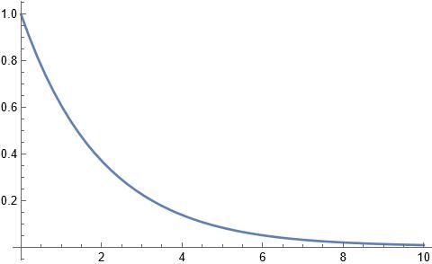
By doing this, we obtain that our result in the Schrödinger representation is a decaying exponential
Solving this system analytically, we get the same result. It follows that our result agrees with the analytical result.
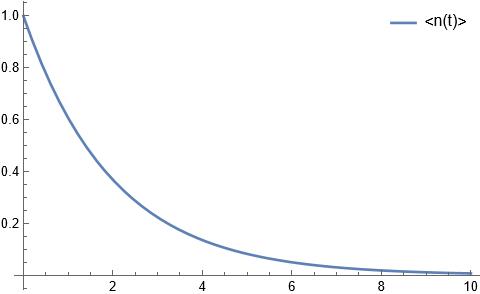
The evolution of the average number of particles is shown in Fig. 1
The same results are obtained for the average linear operators.
We can also compare these results for the case when the higher order moments in Eq. (22) are written out via Wick’s theorem.
5 Weak external field
In this section we consider the case when an external field is present in the system, i.e. . However, considering the general case is a difficult task due to the large number of summands in the oscillator, so we consider the case where the external field is small and the summands with , can be neglected.
| (26) | ||||
where
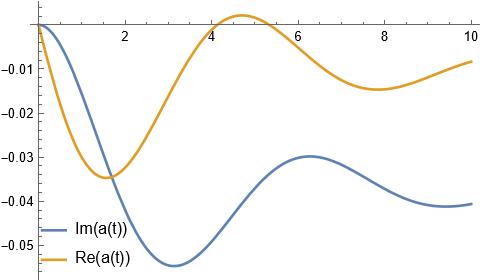
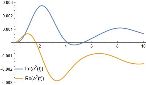
In this case, the action of the conjugate oscillator on an expression of type has the form
| (27) |
where
As we see, in this case such operator does not give an identical 0 when acting on the particle number operator.
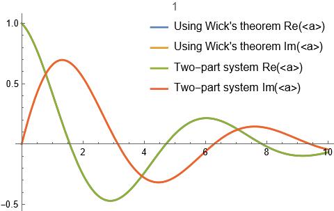
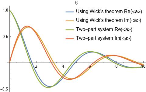
We can also compare the difference between our method and the method using only Wick’s theorem in Eq. (22). This can be done by calculating our equation with . Once we have done this, we can compare the results. The results are presented in Fig. 9 9 9.
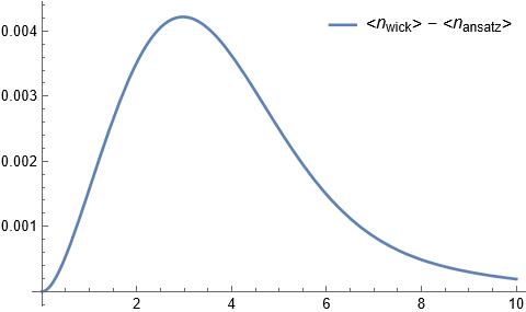
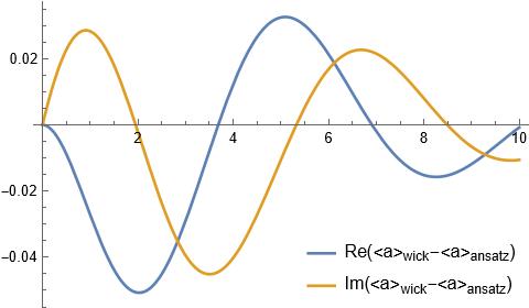
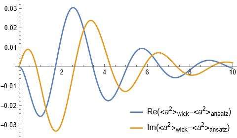
As can be seen, the results are of order .
6 Conclusions
In this work, we have focused on obtaining the Gaussian approximation for the one-mode Kerr model in the external classical field with dissipation. But let us remark that the proposed technique is general and can be applied to multi-mode dissipative models, whose free dynamics preserves the Gaussian states. The specific choice of the model allows us to verify it in the regime, when it is exactly solvable with non-Gaussian solutions. So it can be used as a benchmark of our approach in such an ”uncomfortable” case for it. And, at the same time, our approach allows us to obtain the dynamics for this model in the case, when it is not exactly solvable. This demonstrates the usefulness of our technique.
As an obvious direction for the future study we should mention the application of our approach to other specific models, especially multimode ones. Most of our general calculations are already done in multimode case. And the specific calculations for the discussed model do not seem to complicate much in the multimode case for any reasonable finite number of modes.
The other direction for the future study is to approximate the solution by the finite linear combinations of Gaussian states and applying our equations to each term in the combination separately. In case of non-convex linear combinations, it may allow one to take some non-Gaussian quantum effects into account.
7 Acknowledgments
The authors are grateful to A.Yu. Karasev, A.M. Savchenko, R. Singh, S.D. Mostovoy, A.S. Trushechkin and I.V. Volovich for discussion of the problems discussed in the paper.
The work of Kh. Meretukov was supported by the Foundation for the Advancement of Theoretical Physics and Mathematics “BASIS” under the grant № 23-2-1-34-1.
References
- [1] Dusan Lorenc and Zhanybek Alpichshev. Dispersive effects in ultrafast nonlinear phenomena: The case of optical kerr effect. Physical Review Research, 6(1):013042, 2024.
- [2] Muhammad Asjad, Berihu Teklu, and Matteo GA Paris. Joint quantum estimation of loss and nonlinearity in driven-dissipative kerr resonators. Physical Review Research, 5(1):013185, 2023.
- [3] Junqiu Liu, Guanhao Huang, Rui Ning Wang, Jijun He, Arslan S Raja, Tianyi Liu, Nils J Engelsen, and Tobias J Kippenberg. High-yield, wafer-scale fabrication of ultralow-loss, dispersion-engineered silicon nitride photonic circuits. Nature communications, 12(1):2236, 2021.
- [4] SP Nikitin and AV Masalov. Quantum state evolution of the fundamental mode in the process of second-harmonic generation. Quantum Optics: Journal of the European Optical Society Part B, 3(2):105, 1991.
- [5] JF Corney and MK Olsen. Non-gaussian pure states and positive wigner functions. Physical Review A, 91(2):023824, 2015.
- [6] Lance G Joneckis and Jeffrey H Shapiro. Quantum propagation in a kerr medium: lossless, dispersionless fiber. JOSA B, 10(6):1102–1120, 1993.
- [7] Arup Banerjee. Interaction of squeezed light with a kerr medium. Quantum Optics: Journal of the European Optical Society Part B, 5(1):15, 1993.
- [8] Marco G Genoni, Carmen Invernizzi, and Matteo GA Paris. Enhancement of parameter estimation by kerr interaction. Physical Review A—Atomic, Molecular, and Optical Physics, 80(3):033842, 2009.
- [9] R Román-Ancheyta, M Berrondo, and J Récamier. Parametric oscillator in a kerr medium: evolution of coherent states. JOSA B, 32(8):1651–1655, 2015.
- [10] E Bolandhemmat and F Kheirandish. Quantum dynamics of a driven parametric oscillator in a kerr medium. Scientific Reports, 13(1):9056, 2023.
- [11] Raphaël Menu and Tommaso Roscilde. Gaussian-state ansatz for the non-equilibrium dynamics of quantum spin lattices. SciPost Physics, 14(6):151, 2023.
- [12] Alexander S Holevo. Quantum systems, channels, information: a mathematical introduction. Walter de Gruyter GmbH & Co KG, 2019.
- [13] Kyozi Kawasaki and James D Gunton. Theory of nonlinear transport processes: Nonlinear shear viscosity and normal stress effects. Physical Review A, 8(4):2048, 1973.
- [14] Jochen Rau and Berndt Müller. From reversible quantum microdynamics to irreversible quantum transport. Physics Reports, 272(1):1–59, 1996.
- [15] Vitalii Semin and Francesco Petruccione. Dynamical and thermodynamical approaches to open quantum systems. Scientific reports, 10(1):2607, 2020.
- [16] Kh Sh Meretukov and AE Teretenkov. On time-dependent projectors and a generalization of the thermodynamical approach in the theory of open quantum systems. Proceedings of the Steklov Institute of Mathematics, 324(1):135–152, 2024.
- [17] AE Teretenkov. Irreversible quantum evolution with quadratic generator. Infinite Dimensional Analysis, Quantum Probability and Related Topics, 22(04):1930001, 2019.
- [18] Iu A Nosal and AE Teretenkov. Higher order moments dynamics for some multimode quantum master equations. Lobachevskii Journal of Mathematics, 43(7):1726–1739, 2022.
8 Appendix
Let us write out some of the beneficial properties of the Gaussian ansatz.
Theorem 1.
The proof can be found in [17].
This feature allows us to carry the density matrix through the quadratic form of the creation/annihilation operators.
However, the main feature that is the reason we use the Gaussian ansatz is Wick’s theorem.
Theorem 2.
For a Gaussian ansatz with zero mean and with the matrix of second moments it follows that
The proof of this theorem and more details can be found in [18]
Theorem 3.
The generator in the Heisenberg representation has the form
Proof.
The operator can be represented as , then
Since the trace is invariant with respect to cyclic permutations, then
hence the operator is represented in the form
The operator can be rewritten as
hence
Thus we get the desired result.
Theorem 4.
The derivative of the Gaussian exponent can be expressed as a quadratic form
where
where , in which and — covariance matrix.
Proof.
Using the formula , we can explicitly write .
then
In a similar way, we can simplify the vector
where
| (29) |
Theorem 5.
where
Proof.
where
Then