Combining Causal Discovery and Machine Learning for Modeling Data Center Operations

Abstract.

Data centers consume large amounts of energy, and their electricity demand is predicted to multiply in the coming years. To mitigate the growing environmental challenges associated with data center energy consumption, optimizing the operation of IT equipment (ITE) and Heating, Ventilation, and Air Conditioning (HVAC) systems is crucial. Yet, modeling such systems is challenging due to the complex and non-linear interactions between many factors, including server load, indoor climate, weather, and data center configurations. While physical simulations are capable of representing this complexity, they are often time-consuming to set up and run. Machine Learning (ML), in contrast, allows efficient data-driven modeling but typically does not consider a system’s causal dynamics, lacks interpretability, and suffers from overfitting. This study addresses the limitations of ML-driven predictive modeling by employing Causal Discovery to select features that are causally related to the response variable. We use a simulated data center to generate time series of its operation and conduct experiments to compare ML models trained with all features, traditional feature selection methods, and causal feature selection. Our results show that causal feature selection leads to models with substantially fewer features and similar or better performance, especially when predicting the effects of interventions. In addition, our proposed methodology allows the interpretation of the causal mechanism and the integration of expert knowledge into the modeling process. Overall, our findings suggest that combining Causal Discovery with ML can be a promising alternative for feature selection methods and prediction of interactions in complex physical systems.

1. Introduction

Data centers are the backbone of the global digital economy, and their importance is expected to rise sharply with the increasing adoption of Artificial Intelligence and related technologies (Masanet et al., 2020; Liu et al., 2020). However, this growth also introduces significant climate-related challenges. In 2016, data centers consumed approximately 200 Terawatt-hours of electricity—equivalent to the annual consumption of South Africa (Worldometers.info, 2024). By 2030, this demand is projected to increase two- to threefold (Koot and Wijnhoven, 2021), paralleling the energy consumption forecast for the entire African continent (Ahmad and Zhang, 2020). Optimizing data center operations is therefore a critical challenge for the coming years.

Data centers are complex systems characterized by numerous elements with non-linear interactions that make accurate modeling difficult. For instance, variables such as weather conditions, IT load, internal server room temperatures, and their combined impact on IT equipment (ITE) power consumption and Heating, Ventilation, and Air Conditioning (HVAC) systems create a dynamic and challenging environment (Jin et al., 2020; Sun et al., 2021).

Physical simulations have been commonly used to represent and analyze data center complexities. While effective, these methods are time-consuming and difficult to scale across real-world data centers. As data centers increasingly collect vast amounts of operational data, Machine Learning (ML) has emerged as a valuable tool for data-driven modeling and forecasting, particularly in areas such as temperature, load, and energy consumption prediction (Zhang et al., 2021; Jin et al., 2020). Nonetheless, the large number of variables relevant for data center operations, coupled with many interactions and non-linear relationships, often leads to overly complex ML models that are difficult to interpret and prone to overfitting (Zhang et al., 2021). Moreover, ML models typically fail in predicting out-of-distribution situations, which makes them unsuitable for answering hypothetical ”what-if” questions (e.g., What would be the effect of operating data centers in broader temperature ranges on their energy consumption?) (Zhang et al., 2023).

While explainable AI (XAI) techniques can be used to shed some light on black-box ML models (Lundberg and Lee, 2017), these methods still rely on the predictive capabilities of ML models and often fail to uncover the underlying causal dynamics within the system (Lundberg et al., 2021). As a result, ML models that do not account for the system’s causal structure may suffer from issues such as confounding bias (Hamdan et al., 2023) and struggle to predict the effects of interventions (Schölkopf, 2022), such as adjusting control variables in a data center.

This study addresses these challenges by applying causal discovery methods to uncover causal relationships between variables in data center operations, enabling the selection of features that are causally related to the response variable. Focusing on causality, promises simpler and more interpretable models that can provide robust predictions. A causal discovery-based ML approach also allows to integrate domain knowledge directly into the modeling process.

We present a comprehensive case study that demonstrates the application of causal discovery methods to identify causal relationships among variables in a simulated data center environment. This approach allows us to perform feature selection on time-series data with the integration of domain expertise. We then train ML models using both causal and non-causal features, conducting experimental evaluations on predictive performance across 100 simulations of data center operations with interventions (e.g., changing cooling set points).

Our findings show that ML models trained with causal features performed as well as or better than those trained using traditional non-causal feature selection methods, particularly in predicting the outcomes of interventions. Moreover, the models based on causal features required significantly fewer predictors, demonstrating the efficiency of causal feature selection.

These results underscore the advantages of incorporating causality into ML-based modeling of energy systems. By improving transparency and interpretability, causal discovery-based models avoid the pitfalls of confusing correlation and causality and treating data-driven modeling as a ”black-box” process. Notably, models trained with causal features not only require fewer inputs but also maintain performance levels comparable to traditional methods, reducing the computational resources needed for training and inference. Furthermore, causal models are better in predicting the outcomes of interventions, which is essential for addressing ”what-if” scenarios and can be extended to applications such as training Reinforcement Learning agents.

The remainder of this paper is arranged as follows: Section 2 reviews related work ML-based modeling and forecasting in the context of data centers operations, and gives a background on Causal ML for time series data. Section 3 describes the methods for causal discovery and ML-based predictive modeling we used in this study. Section 4 explains our experimental setup and how we evaluated the different models in two scenarios, with all predictions and with focus on interventions. Finally, in Section 5 we discuss our empirical findings and in Sections 6 and 7 we acknowledge limitations of our work, give an outlook for future work, and highlight the conclusions of our study.

2. Background

2.1. Machine Learning-based Predictive Modeling of Data Centers

Predictive modeling of data center operations using Machine Learning (ML) techniques is well established in the literature, particularly for predicting electricity consumption of IT equipment, server room temperatures, and IT workloads. Jin et al. (2020), for example, reviewed various ML-based power consumption models for data center servers, including both linear and non-linear approaches. Among other findings, they determined that energy- and thermal-aware management, based on accurate power consumption models, achieves the most effective energy savings in data centers. Similarly, Deepika and Prakash (2020) fitted multiple regression models—such as Lasso, Ridge, Elastic Net, Random Forest, K-Nearest Neighbors, and Multi-layer Perceptron (MLP)—to predict power consumption in Azure Virtual Machines and have less uncertainty in power management. They found that the MLP was the model with the best performance. Focusing on temperature predictions, Lin et al. (2022) simulated an air-cooled data center and compared the predictive accuracy of six ML models, including Support Vector Regressors, different tree-based models, Artificial Neural Networks (ANNs), and Long Short-Term Memory (LSTM) networks. Among these, tree-based models like XGBoost and LightGBM provided the best predictive performance. Similarly, Tabrizchi et al. (2023) collected data from a real-world data center and developed a data-driven temperature prediction method using Convolutional Neural Networks (CNNs) combined with stacked bidirectional Long Short-Term Memory (BiLSTM) networks, achieving the highest R-squared values. In the domain of IT workload prediction, Saxena et al. (2023) performed a classification and taxonomy of ML-based workload prediction techniques and evaluated them using data from Google Clusters and PlanetLab virtual machines. They compared and showed the performance and trade-offs of various models and outlined that in the future explainable Artificial Intelligence (XAI) methods could be employed to build robust models, with better prediction scores and more transparent.

2.2. Causal Graphical Models for Time Series

Graphical Causal Models (GCMs) provide a visual representation of causal relationships within a system or process, utilizing Directed Acyclic Graphs (DAGs) (Pearl, 2009). In a GCM, variables are depicted as nodes, and the edges between them represent causal relationships. A directed edge from variable A to variable B indicates a direct causal effect, meaning that changes in the value of A will influence the value of B.

There are various characteristic patterns that help analyze causal relationships between variables in a GCM. The most basic one is a chain, where all arrows point in the same direction, such as, $X\rightarrow Z$ or $X\rightarrow Y\rightarrow Z$. In the latter chain, $X$ and $Z$ are conditionally independent given $Y$ ($X\perp\!\!\!\perp Z\mid Y$). If we aim to analyze the effect of $X$ on $Z$, $Y$ acts as a mediator, and controlling for it (e.g., by fixing its value) would block the effect of $X$ on $Z$. A fork is another important pattern that represents a common cause. For instance, in $Y\leftarrow X\rightarrow Z$, $Z$ and $Y$ are conditionally independent given $X$ ($Z\perp\!\!\!\perp Y\mid X$). In this case, X is a confounder and it creates a non-causal association between Y and Z. Controlling for the confounder blocks this association. A collider, where two arrows point to the same node $X\rightarrow Z\leftarrow Y$, represents a common effect. Here, $X$ and $Y$ are conditionally independent ($X\perp\!\!\!\perp Y$) and controlling for $Z$ generates a spurious association between $X$ and $Y$ (Peters et al., 2017).

GCMs are typically used for cross-sectional data. Yet, time series data can also be represented with stationary DAGs (Runge et al., 2023), where the causal relationships between variables do not change over time. Figure 1 (a) shows a summary graph, also called a process graph, in which the edges are annotated with numbers indicating time lags in causal effects. The number under each node indicates that the variables also cause themselves, with lag 1. Figure 1 (b) depicts a time series graph of the same structural causal model, in which time lags are represented as columns. In this format, the acyclic nature of DAGs is more apparent.

Figure 1. Graphs to represent causality in time series

2.3. Causal Discovery in Time Series

A GCM can be constructed using either domain knowledge or causal discovery methods. Causal discovery involves automatically extracting the causal graph from data. There are several families of algorithms for causal discovery (Molak, 2023; Hasan et al., 2023). The most important ones include:

• Constraint-based methods, which rely on variable independence. The most well-known algorithm in this category is the Peter-Clark (PC) algorithm (Spirtes et al., 2001).

• Score-based methods, which use a scoring function, such as the Bayesian Information Criterion (BIC) or Minimum Description Length (MDL), to determine the best graph. A widely used algorithm in this group is Greedy Equivalence Search (Chickering, 2020).

• Gradient-based methods, which treat graph search as an optimization problem. The NOTEARS algorithm is a prominent example in this category (Zheng et al., 2018).

• Functional discovery methods, based on independent component analysis, where variables are expressed as functions of other variables and noise. An example is the Non-Gaussian Acyclic Model (LiNGAM) (Shimizu, 2014).

In this paper, we use a variant of the constrained-based PC algorithm, as it has shown good performance for causal feature selection in the context of time series problems in past studies (Assaad et al., 2022; Runge, 2020).

The PC algorithm (Spirtes et al., 2001) builds upon the faithfulness assumption, stating that all observed statistical independencies in the data reflect the true underlying causal structure of the underlying data-generating process. The algorithm first establishes a fully connected undirected graph and subsequently performs iterative conditional independence tests to delete edges from the initial graph. Specifically, if two variables are conditionally independent given a set of other variables, the edge between them is removed. Finally, the algorithm orients the edges by identifying colliders (i.e., the only type of relationship where an independence test can determine the direction of the arrows) and disallowing cyclic structures (Glymour et al., 2019). The PC algorithm can be used with different types of conditional independent tests.

In time series data, every variable has an index representing a time lag. Using the PC algorithm directly on such datasets is computationally expensive (every combination of variable and time lag is considered as an individual predictor) and can lead to high false positive rates. To overcome these problems, a variant of the original PC algorithm called the $\text{PC}_{1}$, has been developed that performs the iterative independence test only on the most relevant lagged variables (Beucler et al., 2023; Runge et al., 2019a).

Causal methods for time series rely on several key assumptions. These include the **Causal Markov Condition**, which states that, except for its direct descendants, a variable is independent of all others given its direct causes; **causal sufficiency**, which assumes there are no hidden or unobserved confounders; and **stationarity**, which requires that the statistical and causal properties of the data remain constant over time. In practice, it is often difficult to avoid violations of these assumptions, leading to potential false-positive or false-negative causal links (Runge, 2018a; Hasan et al., 2023; Moraffah et al., 2021; Assaad et al., 2022; Runge, 2018a).

2.4. Using GCMs and ML for Modeling Energy Systems

A GCM, either discovered from data or modeled based on expert domain knowledge, can be used in various ways as input for downstream causal tasks (e.g., identification, estimating causal effects, root-cause analysis) (Sharma and Kiciman, 2020; Blöbaum et al., 2022). In this study, we focus on the task of causal feature selection to enable robust predictions, including situations after interventions into the system.

To illustrate the difference between traditional data-driven predictive modeling and causal prediction, consider the example shown in Figure 1. If the goal is to predict the variable $Y$ at time $t$ (red), a data-driven approach would typically ignore the causal structure of the system, feeding a combination of all observed variables and their time lags as features into an ML model. In this case, the model might identify $Z_{t-1}$ as an important feature, even though its association with $Y_{t}$ is spurious, caused by the confounding effect of $X_{t-2}$. In contrast, a causal prediction approach would only include the causally related variables from previous lags as predictors (blue) and disregard unrelated variables (e.g., $Z$) and time lags (e.g., $t$). This method is likely to enhance the robustness of the predictive model, particularly in scenarios involving data distribution shifts or interventions. Additionally, feeding causal variables as features into flexible, non-parametric ML models, as opposed to traditional statistical approaches (e.g., additive linear models), typically allows for more accurate models that account for non-linearities and interactions.

The combination of causal discovery and ML is gaining traction in the modeling of complex energy systems. For example, He et al. (2019) proposed a causality-based feature selection method by cardinality-constrained direct information maximization and a greedy algorithm for streaming feature selection to detect power system events. They compared their approach to using all the features and to a minimum Redundancy - Maximum Relevance (mRMR) feature selection method and showed that their approach improves detection accuracy by 5% while reducing computational time. Also, Chen et al. (2022) proposed a four-step framework to discover causal relationships from interventions in the energy-efficient building design context, stating that causal discovery allows integrating domain knowledge and achievs a better performance than purely data-driven machine learning methods for answering what-if questions. In the context of data centers, Nandwana et al. (2018) used Granger causality tests on simulated data to determine the influence of air flow rate, supply air temperature, and IT-Load on temperature changes between hot and cold aisles. They later used this information to determine the hot spots in data centers and found that they were similar to the results of physical simulations.

3. Methods

Our proposed approach for robust causal predictions involves two phases: (1) causal discovery to identify variables and time lags that are causally related to the response, and (2) using the identified variable-lag combinations as features in a traditional supervised ML model.

In the first phase, we use the Python library Tigramite (time-series graph-based measures of information transfer), a causal discovery framework for time-series data that relies on conditional independence tests (Runge, 2018a). Following the causal inference method selector from Runge et al. (2023), we first test for stationarity using the Augmented Dickey-Fuller test from the Statsmodels library (Seabold and Perktold, 2010) with a p-value threshold of 0.01. If necessary, we apply differencing (i.e., subtracting the previous value from the current one) to achieve stationarity. Assuming a stochastic system with no hidden confounders, we employ the $\text{PC}_{1}$ algorithm with partial correlation tests and a significance level of 0.01 to discover the GCM (Beucler et al., 2023). For the $\text{PC}_{1}$ algorithm, we specify a maximum lag $\tau_{\text{max}}$ for performing the causality tests, using the average maximum lagged unconditional dependencies (lagged correlations) between all variables within a specific time period (Saetia et al., 2021; Runge et al., 2019b). We visualize the resulting GCM and, if necessary, refine it based on domain knowledge.

To extract causal features from the GCM, we use two approaches. In the Causal-lags approach, we select only those variable-lag combinations that are present in the GCM. In the Causal-all approach, we select all variables with at least one causal link to the response variable, including all lags for those variables. As a baseline, we use all variables with all lags. Additionally, we apply various non-causal feature selection methods from the scikit-learn library (Pedregosa et al., 2011) for comparison. Table 1 summarizes the evaluated causal and non-causal feature selection methods.

In the second phase, we input the selected features from the training set into several regression models, including Linear Regression (LR) and Multilayer Perceptron Regressor (MLP) from the Scikit-learn library (Pedregosa et al., 2011), XGBRegressor (XGB) from the Xgboost library (Chen and Guestrin, 2016), and LGBMRegressor (LGBM) from the LightGBM library (Ke et al., 2017). For all models except Linear Regression, we perform hyperparameter tuning using random search and cross-validation ($K=3$). Finally, we evaluate the predictive accuracy of the models on the test set.

Figure 2 provides an overview of our pipeline for (causal) feature selection, ML training, and evaluation. Blue lines depict data flows, orange lines represent the flow of feature names, and red and violet lines indicate models and results, respectively.

Table 1. Causal and traditional Feature Selection Methods

Algorithm	Description
Recursive Feature Elimination (RFE)	Uses a LinearRegression to remove the least important features recursively.
Principal Component Analysis (PCA)	Reduces the dimensionality by transforming the features into a set of linearly uncorrelated components. The number of components is chosen to explain an 85% of variance. Features are selected based on the importance derived from the PCA.
Tree-based (TB)	Uses a RandomForestRegressor, to estimate feature importance. Features with importance scores above 0.01 are selected.
Lasso	Performs L1 regularization to penalize the absolute size of the coefficients. This leads to some coefficients being exactly zero. Features with non-zero coefficients are selected. The alpha value is 0.1.
Causal	Feature name and lag with a directed link to the target variable in a GCM
Causal-all	Variable name with at least one directed link to the target variable in GCM, but with all the lags
All	All variables and lags for the ML modeling

Table 2. Variables in the dataset

Variable	Description	Unit	Mean	Std Dev	Median
$In\_Temp$	Temperature inside the server room	celsius degrees	25.7158	2.0116	25.8532
$In\_Hum$	Humidity level inside the server room	percentage	34.5140	15.8877	38.0513
$HVAC\_Ener$	Energy consumption of HVAC components	kilowatt-hour	3.1475	4.8663	1.1951
$ITE\_Ener$	Energy consumption of CPU and FAN of the IT equipment	kilowatt-hour	38.2815	12.1617	40.7471
$Hour$	The hour of the day	hour	11.5000	6.9226	11.5000
$Out\_Temp$	Temperature of the outdoor environment	celsius degrees	15.7243	10.3482	15.8969
$Out\_Hum$	Humidity level outside the building	percentage	68.6156	20.7683	70.0000
$Out\_Wind$	Wind speed outside the building	meter per second	4.8938	2.4582	4.6000
$Out\_Wind\_Dir$	Wind direction outside the building	degrees	186.9254	105.6507	200.0000
$Cool\_Set$	Desired cooling temperature setpoint	celsius degrees	25.5451	2.2217	25.0000
$IT\_Load$	IT load on the CPUs in the Data Center	percentage	0.5186	0.2837	0.5939

Figure 2. Data pipeline showing the flow of information for Causal Discovery, training and testing

4. Experiments

4.1. Simulation

We used EnergyPlus and Sinergym to simulate the operations of a Data Center (Jiménez-Raboso et al., 2021). EnergyPlus (Crawley et al., 2001) simulation models have been widely validated, and Sinergym enhances usability and reproducibility by integrating with Python and its data science libraries (Manjavacas et al., 2024; Zhang et al., 2019).

The EnergyPlus simulation represents an air-cooled data center with no aisle containment and two asymmetrical standalone zones (East and West). For this study, we focus only on the West zone, which has a total area of 232.26 m². The zone includes a single air loop system, HVAC, an outdoor air system, variable air volume fans, direct and indirect evaporative coolers, direct expansion cooling coils, and no windows (Moriyama et al., 2018). The dominant heat source is the IT Equipment (ITE), although other marginal heat sources, such as illumination, also contribute (Li et al., 2019).

We simulate two full years of data center operations. Each time step in the simulation corresponds to one hour, resulting in a total of 17,472 hours per simulation. The simulations use New York weather data from the EnergyPlus weather files. The simulation is repeated 100 times with variations in both weather conditions and IT loads.

We introduced several interventions during each simulation by adjusting the $Cool\_set$. These deliberate interventions were designed to test how well the different predictive models generalize to abrupt changes in the system (see Section 4.5).

Figure 3. Visualization of the variables in the training dataset for the first simulation

4.2. Exploratory Data Analysis

We split the data from each simulation run into a training set (the first year, 50% of the data) and a test set (the second year, 50% of the data), ensuring a full cycle of four seasons and avoiding temporal leakage. For the visualizations and summary statistics in this paper, we used only the training data from the first simulation run. Table 2 lists the main variables of our simulation, along with their units of measurement and summary statistics.

Figure 3 illustrates the time series for the training set of the first simulation run, the x-axis shows the time steps. Many variables exhibit non-stationary behavior. Therefore, we tested all series for stationarity and converted them to stationary series when necessary, as this is a prerequisite for time-series causal discovery. Some series, such as those involving interventions in the $Cool\_set$, show rapid shifts in mean. Other variables, particularly the $IT\_Load$, display strong cyclical patterns, while the $Out\_Temp$ reflects clear seasonal trends.

The $In\_Temp$, and to a lesser degree $ITE\_Ener$, fluctuate with changes in the $Cool\_set$. Additionally, $IT\_Load$, $In\_Temp$, and $ITE\_Ener$ appear to vary according to the time of day. The $HVAC\_Elec$ demonstrates a marked increase in energy consumption during summer months, when higher $Out\_Temp$ values require the cooling system to use compressors more intensively, resulting in increased energy use.

The pair plot with histograms and kernel density plots in Figure 4 visualizes several bivariate relationships. From a visual inspection of the plot, we observe that $IT\_Load$ correlates positively with both the $Hour$ and $ITE\_Ener$. Additionally, $Cool\_set$ shows a positive correlation with $In\_Temp$, and a weaker positive correlation with $ITE\_Ener$, while exhibiting a negative correlation with $In\_Hum$. Furthermore, $Out\_Temp$ displays a positive correlation with $In\_Hum$.

Figure 4. Distribution and interactions between the variables

4.3. Causal Discovery

For causal discovery, we averaged the training sets from all 100 simulation runs. As outlined in Section 3, we then calculated the maximum lagged correlation between all variables. We tested lags from 1 to 24 and determined the average maximum correlation, $\tau_{\text{max}}$, to be 9. Using this $\tau_{\text{max}}$ and a significance level (alpha) of 0.01, we ran the $\text{PC}_{1}$ algorithm to generate the initial GCM.

Figure 5 (a) displays the resulting initial summary graph. The edge colors represent partial correlations between variables, while the node colors indicate autocorrelation. This initial GCM provides insights into the causal structure of the data-generating process. For example, we can observe that $Cool\_set$ affects $In\_Temp$ after two time steps. However, the initial GCM is not without errors. For instance, it is implausible for $Out\_Hum$ or $ITE\_Ener$ to cause the $Hour$ of the day, or for $HVAC\_Ener$ to cause $IT\_Load$. Additionally, some links are missing. We know, for example, that $In\_Temp$ causally affects $ITE\_Ener$ because higher temperatures increase the energy consumption of built-in CPU fans (Sun et al., 2021), and it similarly impacts $HVAC\_Ener$. Moreover, $Out\_Temp$ affects both $In\_Temp$ and $HVAC\_Ener$. Therefore, we made minor adjustments to the GCM, adding or removing links based on our domain knowledge.

In a static causal graph, editing simply involves adding a link between two variables. However, in a time-series causal graph, we must also specify the appropriate lag. In our case, we select the first lag, as causal effects typically diminish over time, and a data center controlled to maintain a certain $In\_Temp$ will return to stability quickly after any disturbance. This can be observed in Figure 3, where changes to $Cool\_set$ affect $In\_Temp$.

Figure 5 (b) shows the final edited graph. Newly added links are marked in blue, while removed links are marked in red. Although this graph may still not be perfect, it represents the best possible encoding of the system’s causal structure based on the data and knowledge available.

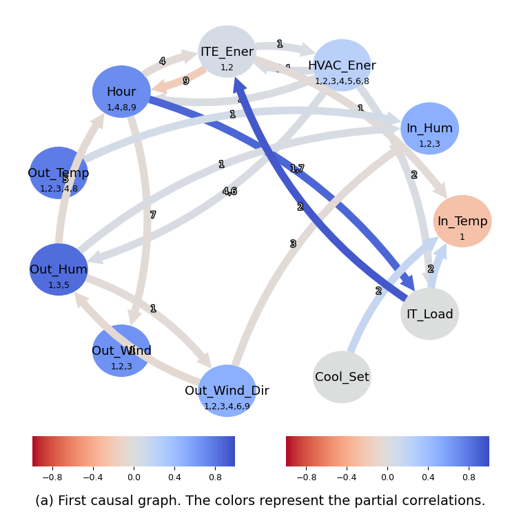
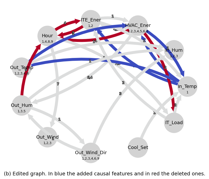
Figure 5. Graphical causal models of the data center operations

4.4. Training and Evaluating ML-based Predictive Models

We selected two different response variables, $ITE\_Ener$ and $In\_Temp$, and trained various regression models using both causal and non-causal features as input. Figure 6 illustrates this process. For the models using the $Causal\_lag$ feature selection method (Figure 6 (a)), we selected only the causally related variable-lag combinations (as determined by the final edited GCM) as predictors. In contrast, for the fully data-driven models (Figure 6 (b)), we used all available variable-lag combinations as predictors.

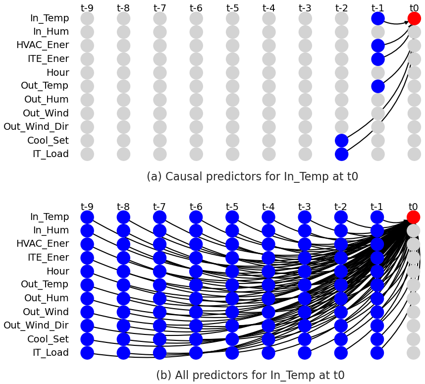
Figure 6. Time series graph with predictors

We begin by comparing the performance of causal versus non-causal feature selection methods over the complete 1-year test set. Each model is trained and evaluated individually for each simulation run, and the results are averaged across all 100 runs. To compare the models, we use the Mean Absolute Error (MAE) as the primary metric, $\text{MAE}=\frac{1}{n}\sum_{i=1}^{n}|y_{i}-\hat{y}_{i}|$, and the Mean Squared Error (MSE), $\text{MSE}=\frac{1}{n}\sum_{i=1}^{n}(y_{i}-\hat{y}_{i})^{2}$, where $y_{i}$ is the actual value of the target variable for index $i$ in the test set, and $\hat{y}_{i}$ is the predicted value. Additionally, we use the Mean Absolute Percentage Error (MAPE), $\text{MAPE}=\frac{100}{n}\sum_{i=1}^{n}\left|\frac{y_{i}-\hat{y}_{i}}{y_{i}}\right|$, which provides a percentage-based measure of predictive accuracy. Our baseline model is a Linear Regression (LR) model that uses all available features.

Table 3. Results for ITE_Ener

Label	Mod	No F	MAE	MSE	MAPE
Causal-all	MLP	36	2.2231	18.0080	6.9975
RFE	MLP	49	2.5203	21.8682	7.8719
Causal-lags	MLP	6	2.6157	24.7522	8.9638
Lasso	MLP	81	2.6258	22.7932	8.1456
All	MLP	99	2.6368	22.3776	8.1733
Causal-all	LGBM	36	2.6540	23.3716	8.4202
Lasso	XGB	81	2.6888	23.6925	8.5102
RFE	XGB	49	2.6895	23.6725	8.5201
Lasso	LGBM	81	2.6997	23.8016	8.5581
All	XGB	99	2.7053	23.9722	8.5877
Causal-all	XGB	36	2.7077	23.7028	8.6141
All	LGBM	99	2.7467	24.1062	8.7530
RFE	LGBM	49	2.7658	24.6282	8.8002
Tree	MLP	6	2.8124	25.8592	8.9841
Causal-lags	LGBM	6	2.8204	25.8348	9.6632
Tree	LGBM	6	2.8726	26.4124	9.2291
Tree	XGB	6	2.8736	26.2305	9.2508
Causal-lags	XGB	6	2.9161	26.8383	10.0508
Causal-lags	LR	6	3.1689	29.2070	11.0601
Causal-all	LR	36	3.3494	29.2645	10.8455
RFE	LR	49	3.3584	29.3120	10.8658
All	LR	99	3.3617	29.2628	10.8710
Lasso	LR	81	3.3648	29.3898	10.8794
Tree	LR	6	3.4348	30.4478	11.2300
PCA	LGBM	6	9.6120	134.5198	34.1501
PCA	XGB	6	9.6538	135.6400	34.3108
PCA	MLP	6	9.6992	137.3896	34.3651
PCA	LR	6	10.0955	146.2633	36.0104

Table 4. Results for In_Temp

Label	Mod	No F	MAE	MSE	MAPE
Causal-lags	MLP	6	0.2101	0.0954	0.8307
Causal-lags	LR	6	0.2174	0.1015	0.8625
Causal-all	XGB	54	0.2233	0.1280	0.8874
RFE	LGBM	49	0.2234	0.1286	0.8894
Causal-all	LR	54	0.2236	0.1036	0.8852
Causal-lags	LGBM	6	0.2242	0.1278	0.8919
RFE	LR	49	0.2244	0.1041	0.8884
Causal-lags	XGB	6	0.2244	0.1300	0.8921
RFE	XGB	49	0.2244	0.1287	0.8931
All	LR	99	0.2246	0.1042	0.8894
Lasso	LR	45	0.2253	0.1060	0.8927
Causal-all	LGBM	54	0.2275	0.1307	0.9049
All	XGB	99	0.2292	0.1310	0.9118
All	LGBM	99	0.2319	0.1352	0.9227
Lasso	XGB	45	0.2342	0.1358	0.9304
Lasso	LGBM	45	0.2385	0.1392	0.9474
Tree	LR	6	0.2399	0.1287	0.9554
RFE	MLP	49	0.2409	0.1234	0.9557
Tree	MLP	6	0.2448	0.1316	0.9723
Lasso	MLP	45	0.2485	0.1243	0.9847
Causal-all	MLP	54	0.2512	0.1327	0.9927
Tree	XGB	6	0.2773	0.1845	1.1063
All	MLP	99	0.2862	0.1630	1.1304
Tree	LGBM	6	0.2866	0.1876	1.1420
PCA	LGBM	6	1.8868	4.7169	7.5102
PCA	XGB	6	1.8875	4.7248	7.5129
PCA	MLP	6	1.8910	4.7519	7.5250
PCA	LR	6	1.8975	4.7325	7.5539

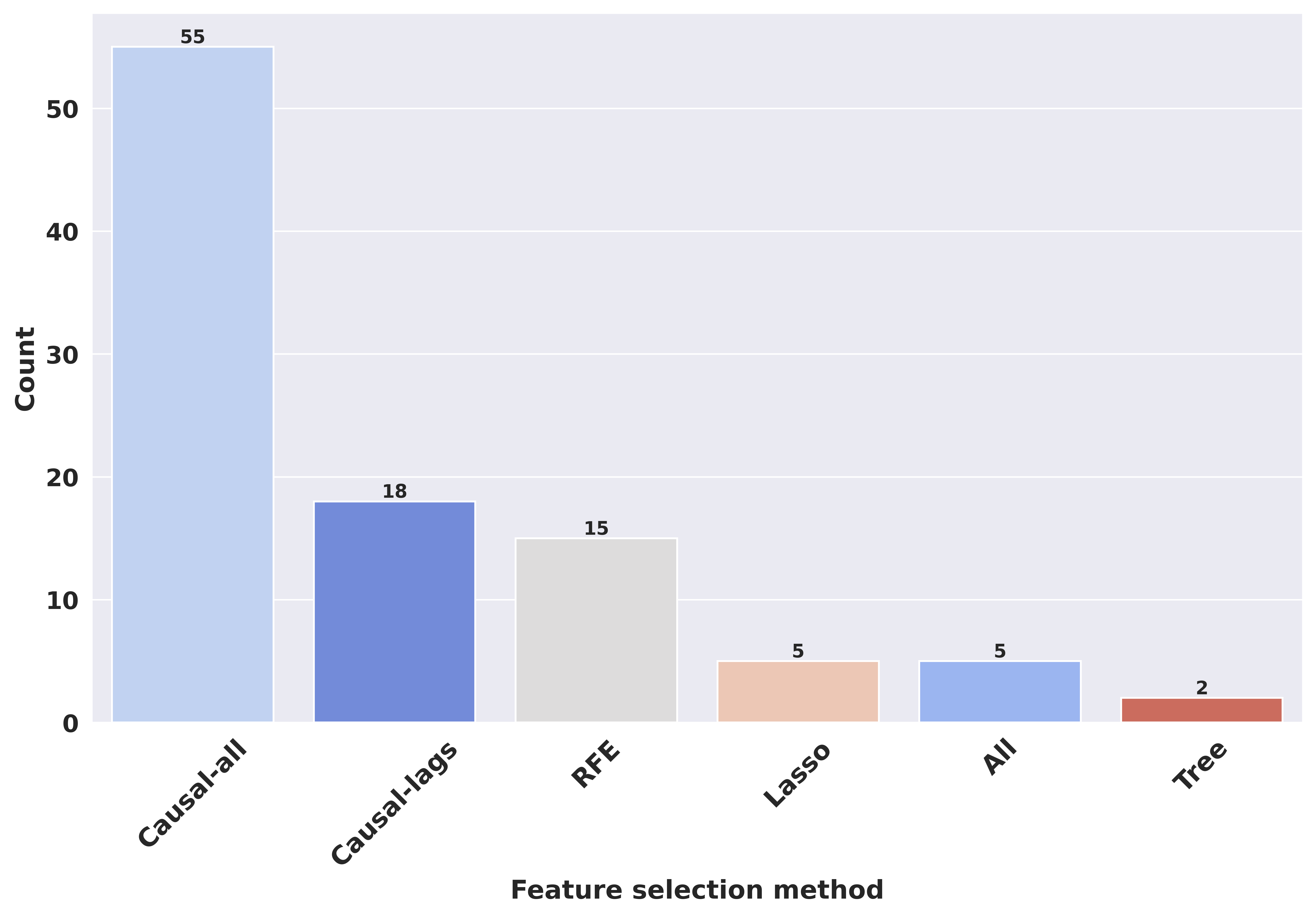
Figure 7. Number of times a feature selection had the best prediction in the simulations’ data for ITE_Ener

Figure 8. Number of times a feature selection had the best prediction in the simulations’ data for In_Temp

Table 4 presents the results of our experiments for the $ITE\_Ener$ response variable, sorted by MAE. The Causal-all feature selection method combined with an MLP clearly outperformed all other models across all metrics, using 36 out of the 99 available features. Figure 8 shows the frequency with which each feature selection method produced the best model: Causal-all was the best 55 times, followed by Causal-lags with 18 and RFE with 15.

Table 4 presents the results for the $In\_Temp$ response variable. In this case, the two causal feature selection methods -Causal-lags with only six features and Causal-all with 54 features- occupy the top three spots. Interestingly, the underlying ML models used for the three best-performing solutions are different: MLP, LR, and XGB. Figure 8 shows that the Causal-lags feature selection method performed the best in 58 simulations, followed by Causal-all with 21 and RFE with 11.

In summary, at this point, it can be concluded that across both prediction tasks, feature selection methods based on causal discovery (i.e., Causal-lags or Causal-all) outperformed other approaches in more than 70% of the simulation runs.

4.5. Predictive Accuracy After Interventions

Causal inference methods are particularly effective when addressing interventional or counterfactual questions (Pearl, 2009). Therefore, we now shift our focus to predictions in scenarios following interventions, such as changes to the cooling set point.

In the simulation, we adjusted the $Cool\_set$ to observe its effect on $In\_Temp$. The $Cool\_set$ was altered on an average of 8 times in both first year (training set) and the second year (test set). Figure 9 (a) shows the time series for $Cool\_set$ and $In\_Temp$ in the test set. The red markers highlight 5 points following a change in $Cool\_set$. The magenta square zooms in on one of these points, as shown in Figure 9 (b). After each change in $Cool\_set$, the $In\_Temp$ begins to change after approximately two time steps. Subsequently, $In\_Temp$ experiences some fluctuations before stabilizing again. While the stabilization behavior varies between different changes in $Cool\_set$ and their corresponding effects on $In\_Temp$, stabilization typically occurs around five time steps after the initial change in $Cool\_set$.

To evaluate model performance following these interventions, we used the trained models from the previous task, but calculated MAE specifically for the window after each change. This is represented as $MAE\textsubscript{w}=MAE_{t+1,...,t+5}$. We did the same for MSE and MAPE.

Table 5 shows that all models performed worse after an intervention on the $Cool\_set$, with MAEs more than doubling compared to the values in Table 4. However, models using causal feature selection now outperformed other approaches even more clearly. In the previous task, the best model trained with causal features for the $In\_Temp$ target was only about 6% better than models trained with all features. In this case, their performance is roughly 17% better compared to the best models using other feature selection methods. Figure 10 reinforces this finding, showing that the Causal feature selection method produced the best model in 80 out of the 100 simulation runs, followed by Lasso with 9.

Figure 11 illustrates how the average MAE for each feature selection method evolves over time following a change in the set point. Immediately after the change, the causal models perform significantly better than the others. However, this difference diminishes as the system stabilizes.

Figure 9. Values of In_Temp after a change in Cool_set

Table 5. Evaluation for every input size and horizon for all datasets

Label	Model	No F	MAEw	MSEw	MAPEw
Causal-lags	MLP	6	0.4292	0.5551	1.7040
Causal-lags	XGB	6	0.4296	0.5263	1.7141
Causal-lags	LGBM	6	0.4307	0.5249	1.7206
Causal-lags	LR	6	0.4463	0.5777	1.7804
RFE	LR	49	0.5151	0.6448	2.0556
Causal-all	LR	54	0.5153	0.6448	2.0569
All	LR	99	0.5160	0.6451	2.0588
Lasso	XGB	45	0.5299	0.6730	2.1158
Lasso	LR	45	0.5303	0.6846	2.1180
Causal-all	XGB	54	0.5329	0.6820	2.1241
Lasso	LGBM	45	0.5357	0.6749	2.1396
Tree	LR	6	0.5360	0.7075	2.1458
RFE	XGB	49	0.5366	0.6949	2.1406
RFE	LGBM	49	0.5370	0.6943	2.1442
Causal-all	LGBM	54	0.5386	0.6964	2.1494
All	XGB	99	0.5394	0.6913	2.1528
All	LGBM	99	0.5439	0.6949	2.1713
Tree	LGBM	6	0.5601	0.7180	2.2420
Tree	XGB	6	0.5617	0.7450	2.2483
Lasso	MLP	45	0.6040	0.7998	2.4115
Causal-all	MLP	54	0.6453	0.9146	2.5778
Tree	MLP	6	0.6575	1.0758	2.5942
RFE	MLP	49	0.6690	0.9820	2.6729
All	MLP	99	0.6838	0.9564	2.7257
PCA	XGB	6	1.7118	4.1843	6.8868
PCA	LGBM	6	1.7129	4.1890	6.8896
PCA	LR	6	1.7172	4.1950	6.9073
PCA	MLP	6	1.7229	4.2326	6.9279

Figure 10. Number of times a feature selection had the best prediction in the simulations’ data for In_Temp after a change point

Figure 11. Time Series graph with predictors

5. Discussion

In this paper, we used causal discovery for understanding the causal dynamics of data center operations and selecting causally related features for predicting data center energy consumption and server room temperatures. Our experiments suggest that causal feature selection (either selecting all lags for causally related features or only those with partial dependencies) improves the predictive accuracy of forecasting models, especially for situations after an intervention.

A causal discovery process should ideally detect all causal relationships in a system, but in practice, the assumption might be partially violated, and the causal graph can have errors. This was the case in our experiments; yet, causal discovery allows integrating expert knowledge into the process, which we did to edit the graphical causal model. Such a step allows the discussion about the possible causal influences for better interpretation of the data at hand and the incorporation of expert knowledge. All this before starting with an expensive ML modeling.

In contrast to a causal discovery in static use cases like in (Chen et al., 2022), time series data poses a new challenge when editing a causal graph, namely the selection of the correct lag. In our case, we used the first lag, since data centers HVACs are programmed to quickly stabilize the room temperature after disturbances or intervention. Yet, this might not necessarily be the case in other systems. Other solutions could be to set a lower alpha value for the independence test of the $\text{PC}_{1}$ algorithm, or selecting the lags with the strongest correlations. In practice, this design decision will still be subject to the final approval of the analyst or manager.

Our experiments revealed that causal discovery performed as well as or even better than using all available features or using traditional feature selection methods. This findings supports the results of Beucler et al. (2023). We think that this finding is remarkable when considering that the models only used a fraction of the available features, drastically reducing the computational needs of the model fitting process and improving both model interpretability and simplicity.

Especially when predicting the effects of interventions in the system, such as adjusting the $Cool\_set$ and its impact on $In\_Temp$, the causal prediction approaches outperformed all the other methods. This highlights the robustness of causal models in handling interventions and shows the advantages of training ML models based on the causal structure of a system. The approach is especially important when the focus of the model is to serve as a base for answering causal questions and guiding policy, including what-if scenarios or counterfactuals, which is not recommended or not even possible with correlation-based models (Lundberg and Lee, 2017).

Another contribution of our study is the proposal of the Causal-all approach, which uses variables with at least one causal link in the GCM, but then adds these variables with all the lags as features. The strategy is an alternative way of enhancing ML models with causal discovery. This approach outperformed many other feature selection methods for the prediction of $ITE\_Ener$ and was the second-best method for the $In\_Temp$. Yet, tn the case of interventions, this method was worse than the models with only causal features (causal-lags), supporting the recommendation to do more fine-grained causal when answering interventional questions.

Based on our experimental results, we strongly believe that causal machine learning can be an option to model a real system based on historical data with few interventions. This can be an alternative to building expensive simulations to, for example, train a Reinforcement Learning (RL) agent for controlling the system.

6. Limitations and future work

A limitation of our analysis, and of applying causal discovery in practice, is the lack of ground truth for the causal graph. Expert knowledge can be used to edit and improve the causal graph, but the results might not be always ideal. If the causal graph were perfectly accurate, the performance of the ML models with the causal features would be better. Additionally, the library Tigramite (Runge, 2018a) offers more conditional independence tests that were not tested, as well as non-parametric, at the cost of higher computational expenses (Runge, 2018b).

Numerous directions exist for future research on combining causal discovery with data-driven machine learning, especially within the context of data centers. First, practitioners could use real-world data from the operations of a data center, using the same approach the causal models can be evaluated with real systems. In the case of interventional questions, this might be more challenging in real-world applications than in simulations, but is definitely required for validating and replicating our results. Second, it would be interesting to replicate our methodology with varying amounts of data available. We hypothesize that causal models perform better than purely data-driven methods in situations with only little data. Third, causality-based models can be used as a base to train RL agents, comparing them with non-causal models and using them as the benchmark for direct training with simulations.

7. Conclusions

We used a simulation of data center operations with the Sinergym framework (Jiménez-Raboso et al., 2021), which integrates EnergyPlus building simulations with Python controllers. In a simulation, we generated data for two consecutive years of data center operations and repeated this process for 100 simulations varying weather conditions and IT loads.

We presented a method for exploratory causal analysis by using causal discovery and discussing the challenges in the process, such as editing a causal graph and selecting the causal features. Additionally, we demonstrated how this approach enables the integration of domain knowledge, enhancing the overall modeling process and understanding of the physical system.

Later, we trained ML models with causal features and other feature selection methods. The evaluation of the models revealed that causal models require drastically fewer features and have comparable prediction performance with models that use all features and other feature selection models. Furthermore, in the case of predictions after interventions, the causal models considerably outperform all other models. The results of this study highlight the advantages in transparency and simplicity of combining causality with ML, particularly when aiming to predict the outcomes of interventions.

8. Data availability

The authors can share the data upon request.

References

- (1)
- Ahmad and Zhang (2020) Tanveer Ahmad and Dongdong Zhang. 2020. A critical review of comparative global historical energy consumption and future demand: The story told so far. Energy Reports 6 (2020), 1973–1991.
- Assaad et al. (2022) Charles K Assaad, Emilie Devijver, and Eric Gaussier. 2022. Survey and evaluation of causal discovery methods for time series. Journal of Artificial Intelligence Research 73 (2022), 767–819.
- Beucler et al. (2023) Tom Beucler, Frederick Iat-Hin Tam, Milton S Gomez, Jakob Runge, Andreas Gerhardus, et al. 2023. Selecting robust features for machine-learning applications using multidata causal discovery. Environmental Data Science 2 (2023), e27.
- Blöbaum et al. (2022) Patrick Blöbaum, Peter Götz, Kailash Budhathoki, Atalanti A. Mastakouri, and Dominik Janzing. 2022. DoWhy-GCM: An extension of DoWhy for causal inference in graphical causal models. arXiv preprint arXiv:2206.06821 (2022).
- Chen and Guestrin (2016) Tianqi Chen and Carlos Guestrin. 2016. XGBoost: A Scalable Tree Boosting System. In Proceedings of the 22nd ACM SIGKDD International Conference on Knowledge Discovery and Data Mining (San Francisco, California, USA) (KDD ’16). Association for Computing Machinery, New York, NY, USA, 785–794. https://doi.org/10.1145/2939672.2939785
- Chen et al. (2022) Xia Chen, Jimmy Abualdenien, Manav Mahan Singh, André Borrmann, and Philipp Geyer. 2022. Introducing causal inference in the energy-efficient building design process. Energy and Buildings 277 (Dec. 2022), 112583. https://doi.org/10.1016/j.enbuild.2022.112583 arXiv:2203.10115 [cs, stat].
- Chickering (2020) Max Chickering. 2020. Statistically efficient greedy equivalence search. In Conference on Uncertainty in Artificial Intelligence. Pmlr, 241–249.
- Crawley et al. (2001) Drury B Crawley, Linda K Lawrie, Frederick C Winkelmann, Walter F Buhl, Y Joe Huang, Curtis O Pedersen, Richard K Strand, Richard J Liesen, Daniel E Fisher, Michael J Witte, et al. 2001. EnergyPlus: creating a new-generation building energy simulation program. Energy and buildings 33, 4 (2001), 319–331.
- Deepika and Prakash (2020) T Deepika and P Prakash. 2020. Power consumption prediction in cloud data center using machine learning. Int. J. Electr. Comput. Eng.(IJECE) 10, 2 (2020), 1524–1532.
- Glymour et al. (2019) Clark Glymour, Kun Zhang, and Peter Spirtes. 2019. Review of causal discovery methods based on graphical models. Frontiers in genetics 10 (2019), 524.
- Hamdan et al. (2023) Sami Hamdan, Bradley C Love, Georg G von Polier, Susanne Weis, Holger Schwender, Simon B Eickhoff, and Kaustubh R Patil. 2023. Confound-leakage: confound removal in machine learning leads to leakage. GigaScience 12 (2023), giad071.
- Hasan et al. (2023) Uzma Hasan, Emam Hossain, and Md Osman Gani. 2023. A survey on causal discovery methods for iid and time series data. arXiv preprint arXiv:2303.15027 (2023).
- He et al. (2019) Miao He, Weixi Gu, Yuxun Zhou, Ying Kong, and Lin Zhang. 2019. Causal feature selection for physical sensing data: A case study on power events prediction. In Adjunct Proceedings of the 2019 ACM International Joint Conference on Pervasive and Ubiquitous Computing and Proceedings of the 2019 ACM International Symposium on Wearable Computers. 565–570.
- Jiménez-Raboso et al. (2021) Javier Jiménez-Raboso, Alejandro Campoy-Nieves, Antonio Manjavacas-Lucas, Juan Gómez-Romero, and Miguel Molina-Solana. 2021. Sinergym: a building simulation and control framework for training reinforcement learning agents. In Proceedings of the 8th ACM international conference on systems for energy-efficient buildings, cities, and transportation. 319–323.
- Jin et al. (2020) Chaoqiang Jin, Xuelian Bai, Chao Yang, Wangxin Mao, and Xin Xu. 2020. A review of power consumption models of servers in data centers. Applied Energy 265 (May 2020), 114806. https://doi.org/10.1016/j.apenergy.2020.114806
- Ke et al. (2017) Guolin Ke, Qi Meng, Thomas Finley, Taifeng Wang, Wei Chen, Weidong Ma, Qiwei Ye, and Tie-Yan Liu. 2017. Lightgbm: A highly efficient gradient boosting decision tree. Advances in neural information processing systems 30 (2017).
- Koot and Wijnhoven (2021) Martijn Koot and Fons Wijnhoven. 2021. Usage impact on data center electricity needs: A system dynamic forecasting model. Applied Energy 291 (2021), 116798.
- Li et al. (2019) Yuanlong Li, Yonggang Wen, Dacheng Tao, and Kyle Guan. 2019. Transforming cooling optimization for green data center via deep reinforcement learning. IEEE transactions on cybernetics 50, 5 (2019), 2002–2013.
- Lin et al. (2022) Jianpeng Lin, Weiwei Lin, Wenjun Lin, Jiangtao Wang, and Hongliang Jiang. 2022. Thermal prediction for air-cooled data center using data driven-based model. Applied Thermal Engineering 217 (2022), 119207.
- Liu et al. (2020) Yanan Liu, Xiaoxia Wei, Jinyu Xiao, Zhijie Liu, Yang Xu, and Yun Tian. 2020. Energy consumption and emission mitigation prediction based on data center traffic and PUE for global data centers. Global Energy Interconnection 3, 3 (2020), 272–282.
- Lundberg et al. (2021) Scott Lundberg, Eleanor Dillon, Jacob LaRiviere, Jonathan Roth, and Vasilis Syrgkanis. 2021. Be careful when interpreting predictive models in search of causal insights; SHAP latest documentation — shap.readthedocs.io. https://shap.readthedocs.io/en/latest/example_notebooks/overviews/Be%20careful%20when%20interpreting%20predictive%20models%20in%20search%20of%20causal%20insights.html [Accessed 25-08-2024].
- Lundberg and Lee (2017) Scott M Lundberg and Su-In Lee. 2017. A unified approach to interpreting model predictions. Advances in neural information processing systems 30 (2017).
- Manjavacas et al. (2024) Antonio Manjavacas, Alejandro Campoy-Nieves, Javier Jiménez-Raboso, Miguel Molina-Solana, and Juan Gómez-Romero. 2024. An experimental evaluation of deep reinforcement learning algorithms for HVAC control. Artificial Intelligence Review 57, 7 (2024), 173.
- Masanet et al. (2020) Eric Masanet, Arman Shehabi, Nuoa Lei, Sarah Smith, and Jonathan Koomey. 2020. Recalibrating global data center energy-use estimates. Science 367, 6481 (2020), 984–986.
- Molak (2023) Aleksander Molak. 2023. Causal Inference and Discovery in Python: Unlock the secrets of modern causal machine learning with DoWhy, EconML, PyTorch and more. Packt Publishing Ltd.
- Moraffah et al. (2021) Raha Moraffah, Paras Sheth, Mansooreh Karami, Anchit Bhattacharya, Qianru Wang, Anique Tahir, Adrienne Raglin, and Huan Liu. 2021. Causal inference for time series analysis: Problems, methods and evaluation. Knowledge and Information Systems 63 (2021), 3041–3085.
- Moriyama et al. (2018) Takao Moriyama, Giovanni De Magistris, Michiaki Tatsubori, Tu-Hoa Pham, Asim Munawar, and Ryuki Tachibana. 2018. Reinforcement learning testbed for power-consumption optimization. In Methods and Applications for Modeling and Simulation of Complex Systems: 18th Asia Simulation Conference, AsiaSim 2018, Kyoto, Japan, October 27–29, 2018, Proceedings 18. Springer, 45–59.
- Nandwana et al. (2018) Anurag Nandwana, Rahul Kumar Vij, and Divyasheel Sharma. 2018. Causality-Based Thermal Prediction for Data Center. In 2018 IEEE 23rd International Conference on Emerging Technologies and Factory Automation (ETFA), Vol. 1. 1297–1304. https://doi.org/10.1109/ETFA.2018.8502473 ISSN: 1946-0759.
- Pearl (2009) Judea Pearl. 2009. Causality. Cambridge university press.
- Pedregosa et al. (2011) F. Pedregosa, G. Varoquaux, A. Gramfort, V. Michel, B. Thirion, O. Grisel, M. Blondel, P. Prettenhofer, R. Weiss, V. Dubourg, J. Vanderplas, A. Passos, D. Cournapeau, M. Brucher, M. Perrot, and E. Duchesnay. 2011. Scikit-learn: Machine Learning in Python. Journal of Machine Learning Research 12 (2011), 2825–2830.
- Peters et al. (2017) Jonas Peters, Dominik Janzing, and Bernhard Schölkopf. 2017. Elements of causal inference: foundations and learning algorithms. The MIT Press.
- Runge (2018a) Jakob Runge. 2018a. Causal network reconstruction from time series: From theoretical assumptions to practical estimation. Chaos: An Interdisciplinary Journal of Nonlinear Science 28, 7 (2018).
- Runge (2018b) Jakob Runge. 2018b. Conditional independence testing based on a nearest-neighbor estimator of conditional mutual information. In Proceedings of the Twenty-First International Conference on Artificial Intelligence and Statistics (Proceedings of Machine Learning Research, Vol. 84), Amos Storkey and Fernando Perez-Cruz (Eds.). PMLR, 938–947. https://proceedings.mlr.press/v84/runge18a.html
- Runge (2020) Jakob Runge. 2020. Discovering contemporaneous and lagged causal relations in autocorrelated nonlinear time series datasets. In Conference on Uncertainty in Artificial Intelligence. Pmlr, 1388–1397.
- Runge et al. (2023) Jakob Runge, Andreas Gerhardus, Gherardo Varando, Veronika Eyring, and Gustau Camps-Valls. 2023. Causal inference for time series. Nature Reviews Earth & Environment 4, 7 (2023), 487–505.
- Runge et al. (2019a) Jakob Runge, Peer Nowack, Marlene Kretschmer, Seth Flaxman, and Dino Sejdinovic. 2019a. Detecting causal associations in large nonlinear time series datasets. Science Advances 5, 11 (Nov. 2019), eaau4996. https://doi.org/10.1126/sciadv.aau4996 arXiv:1702.07007 [physics, stat].
- Runge et al. (2019b) J Runge, P Nowack, M Kretschmer, S Flaxman, and D Sejdinovic. 2019b. Detecting causal associations in large nonlinear time series datasets, Sci. Adv., 5, eaau4996.
- Saetia et al. (2021) Supat Saetia, Natsue Yoshimura, and Yasuharu Koike. 2021. Constructing brain connectivity model using causal network reconstruction approach. Frontiers in Neuroinformatics 15 (2021), 619557.
- Saxena et al. (2023) Deepika Saxena, Jitendra Kumar, Ashutosh Kumar Singh, and Stefan Schmid. 2023. Performance analysis of machine learning centered workload prediction models for cloud. IEEE Transactions on Parallel and Distributed Systems 34, 4 (2023), 1313–1330.
- Schölkopf (2022) Bernhard Schölkopf. 2022. Causality for machine learning. In Probabilistic and causal inference: The works of Judea Pearl. 765–804.
- Seabold and Perktold (2010) Skipper Seabold and Josef Perktold. 2010. statsmodels: Econometric and statistical modeling with python. In 9th Python in Science Conference.
- Sharma and Kiciman (2020) Amit Sharma and Emre Kiciman. 2020. DoWhy: An End-to-End Library for Causal Inference. arXiv preprint arXiv:2011.04216 (2020).
- Shimizu (2014) Shohei Shimizu. 2014. LiNGAM: Non-Gaussian methods for estimating causal structures. Behaviormetrika 41, 1 (2014), 65–98.
- Spirtes et al. (2001) Peter Spirtes, Clark Glymour, and Richard Scheines. 2001. Causation, prediction, and search. MIT press.
- Sun et al. (2021) Kaiyu Sun, Na Luo, Xuan Luo, and Tianzhen Hong. 2021. Prototype energy models for data centers. Energy and Buildings 231 (2021), 110603.
- Tabrizchi et al. (2023) Hamed Tabrizchi, Jafar Razmara, and Amir Mosavi. 2023. Thermal prediction for energy management of clouds using a hybrid model based on CNN and stacking multi-layer bi-directional LSTM. Energy Reports 9 (Dec. 2023), 2253–2268. https://doi.org/10.1016/j.egyr.2023.01.032
- Worldometers.info (2024) Worldometers.info. 2024. South Africa Electricity. https://www.worldometers.info/electricity/south-africa-electricity/
- Zhang et al. (2019) Chi Zhang, Sanmukh R Kuppannagari, Rajgopal Kannan, and Viktor K Prasanna. 2019. Building HVAC scheduling using reinforcement learning via neural network based model approximation. In Proceedings of the 6th ACM international conference on systems for energy-efficient buildings, cities, and transportation. 287–296.
- Zhang et al. (2021) Qingxia Zhang, Zihao Meng, Xianwen Hong, Yuhao Zhan, Jia Liu, Jiabao Dong, Tian Bai, Junyu Niu, and M Jamal Deen. 2021. A survey on data center cooling systems: Technology, power consumption modeling and control strategy optimization. Journal of Systems Architecture 119 (2021), 102253.
- Zhang et al. (2023) Yingbo Zhang, Kui Shan, Xiuming Li, Hangxin Li, and Shengwei Wang. 2023. Research and Technologies for next-generation high-temperature data centers–State-of-the-arts and future perspectives. Renewable and Sustainable Energy Reviews 171 (2023), 112991.
- Zheng et al. (2018) Xun Zheng, Bryon Aragam, Pradeep K Ravikumar, and Eric P Xing. 2018. Dags with no tears: Continuous optimization for structure learning. Advances in neural information processing systems 31 (2018).