\Yboxdim

6.5pt\Ylinethick0.4pt aainstitutetext: School of Physics, University of Electronic Science and Technology of China, Chengdu, Sichuan 611731, P. R. China bbinstitutetext: College of Physics and Optoelectronic Engineering, Shenzhen University, Shenzhen 518060, P.R. China ccinstitutetext: CAS Key Laboratory of Theoretical Physics, Institute of Theoretical Physics, Chinese Academy of Sciences, Beijing 100190, P. R. China ddinstitutetext: School of Physical Sciences, University of Chinese Academy of Sciences, Beijing, P. R. China eeinstitutetext: School of Physics, Henan Normal University, Xinxiang 453007, P. R. China

Susy breaking soft terms in the supersymmetric Pati-Salam landscape from Intersecting D6-Branes

Mudassar Sabir b    Adeel Mansha c,d,e    Tianjun Li a    Zhi-Wei Wang mudassar.sabir@uestc.edu.cn adeelmansha@alumni.itp.ac.cn tli@itp.ac.cn zhiwei.wang@uestc.edu.cn
Abstract

We investigate the supersymmetry breaking soft terms for all the viable models in the complete landscape of three-family supersymmetric Pati-Salam models arising from intersecting D6-branes on a 𝕋6/(2×2)superscript𝕋6subscript2subscript2\mathbb{T}^{6}/(\mathbb{Z}_{2}\times\mathbb{Z}_{2}) orientifold in type IIA string theory. The calculations are performed in the general scenario of u𝑢u-moduli dominance with the s𝑠s-moduli turned on, where the soft terms remain independent of the Yukawa couplings and the Wilson lines. The results for the trilinear coupling, gaugino-masses, squared-mass parameters of squarks, sleptons and Higgs depend on the brane wrapping numbers and the susy breaking parameters. We find that unlike the Yukawa couplings which remain unchanged for the models dual under the exchange of two SU(2) sectors, the corresponding soft term parameters only match for the trilinear coupling and the mass of the gluino. This can be explained by the internal geometry where the Yukawa interactions depend only on the triangular areas of the worldsheet instantons while the soft terms have an additional dependence on the orientation-angles of D6-branes in the three two-tori. In the special limit of parameter space we find universal masses for the Higgs and the gauginos.

1 Introduction

In the standard model, quarks and leptons arise from chiral representations of the gauge group SU(3)C×SU(2)L×U(1)YSUsubscript3𝐶SUsubscript2𝐿Usubscript1𝑌\textrm{SU}(3)_{C}\times\textrm{SU}(2)_{L}\times\textrm{U}(1)_{Y}. Intersecting D6-branes in type IIA string theory filling the four-dimensional spacetime and extending into three compact dimensions provide a geometric realization of standard model gauge interactions. Open strings stretched between two intersecting D6-branes act as chiral fermions Berkooz:1996km ; Aldazabal:2000cn . Family replication is readily achieved as branes generically intersect at several points. The four-dimensional gauge couplings are determined by the volumes of the cycles wrapped by D6-branes while the gravitational coupling depends on the total internal volume of the compact dimensions, thus allowing the possibility of having the string scale MSsubscript𝑀SM_{\rm S} parametrically smaller than the Planck scale MPsubscript𝑀PM_{\rm P}. Hierarchical Yukawa couplings arise from open world-sheet instantons, which are suppressed by exp(AijkT)subscript𝐴𝑖𝑗𝑘𝑇\exp(-A_{ijk}T), where Aijksubscript𝐴𝑖𝑗𝑘A_{ijk} represents the area of the triangle formed by the intersections {i,j,k}𝑖𝑗𝑘\{i,j,k\}, and T𝑇T denotes the string tension.

Since interesting Yukawa textures cannot arise from a single stack of D-branes is the reason Nature selected the gauge group of the standard model as a direct product of unitary groups rather than a simple unitary group. Statistically, the configurations of the branes tend to favor direct products of unitary groups constructed from an even number of D-branes within the stack. This preference can be explained by the K-theory conditions Witten:1998cd ; Uranga:2000xp , constrained by mod 4 and thus are easier to satisfy for U(2N)U2𝑁\textrm{U}(2N) with N𝑁N\in\mathbbm{Z}. For example, in trinification models, there is not a single consistent three-family model that satisfies the stringent requirements of 𝒩=1𝒩1\mathcal{N}=1 supersymmetry, tadpole cancellation, and K-theory constraints Mansha:2024yqz . Note that even if the models are consistent under the K-theory, no tadpoles and susy conditions, the viable models with realistic Yukawa textures are extremely difficult to engineer. Consequently, the left-right symmetric Pati-Salam group, SU(4)C×SU(2)L×SU(2)RSUsubscript4𝐶SUsubscript2𝐿SUsubscript2𝑅\textrm{SU}(4)_{C}\times\textrm{SU}(2)_{L}\times\textrm{SU}(2)_{R}, stands out as the most promising option for realistic models.

The model building rules to construct supersymmetric Pati-Salam models on a 𝕋6/(2×2)superscript𝕋6subscript2subscript2\mathbbm{T}^{6}/(\mathbbm{Z}_{2}\times\mathbbm{Z}_{2}) orientifold utilizing intersecting D6-branes with the requirement of 𝒩=1𝒩1\mathcal{N}=1 supersymmetry, no-tadpole constraints and ensuring K-theory conditions were laid out in Cvetic:2004ui ; Blumenhagen:2006ci ; Blumenhagen:2005mu . A similar approach has been applied in more recent studies Li:2019nvi ; Li:2021pxo ; Mansha:2022pnd ; Sabir:2022hko ; Mansha:2023kwq . The complete landscape of consistent three-family 𝒩=1𝒩1\mathcal{N}=1 supersymmetric Pati-Salam models containing 206,752 models has been derived in He:2021gug . There are 33 distinct physical models with distinct gauge coupling relations up to type I and type II T-dualities. In Sabir:2024cgt , we have presented the results of Yukawa couplings for all the feasible models in this landscape, and in Sabir:2024mfv the most realistic model explaining the fermion masses and mixings has been discussed.

In this paper, we investigate the supersymmetry breaking soft terms for all the viable three-family supersymmetric Pati-Salam models in the landscape, focusing on the u𝑢u-moduli dominated scenario with the s𝑠s-moduli turned on. In this setup, the soft terms remain independent of the Yukawa couplings and the Wilson lines. The results for the trilinear coupling, gaugino-masses, squared-mass parameters of squarks, sleptons and Higgs are determined by the D-brane wrapping numbers and the supersymmetry breaking parameters, which include the gravitino mass and the goldstino angles.

For any two models which are dual under the exchange of two SU(2)s, the Yukawa couplings produce identical results, however, the corresponding soft term parameters exhibit notable differences. Specifically, the trilinear coupling and gaugino mass match only within the SU(3)SU3\textrm{SU}(3) sector, whereas the other soft terms, such as the bino, wino and squared masses of squarks and sleptons, differ between the dual models. This discrepancy can be understood from the underlying geometry of the compact space. While the Yukawa interactions depend solely on the triangular area of the worldsheet instantons, the soft terms are influenced by additional factors, including the orientation angles of the D6-branes on the three two-tori. As a result, dual models not only exhibit distinct gauge coupling relations but also feature different gaugino masses and soft scalar mass parameters. Since the scale of supersymmetry breaking is still unknown, we mainly focus on generic results in the present work. Nonetheless, we have found an interesting regime of parameters where all gaugino-masses become degenerate and the Higgs mass parameter is half the gravitino-mass which determines the susy breaking scale. This special limit corresponds to fixing three goldstino angles Θ1,2,3=1/2subscriptΘ12312\Theta_{1,2,3}=1/2 and fixing dilaton angle Θs=1/2subscriptΘ𝑠12\Theta_{s}=-1/2, with all CP-violating phases γ1,2,3,ssubscript𝛾123𝑠\gamma_{1,2,3,s} set to zero.

The contents of the paper are organized as follows. In section 2 we briefly review the rules to construct supersymmetric Pati-Salam models from stacks of intersecting D6-branes on a 𝕋6/(2×2)superscript𝕋6subscript2subscript2\mathbbm{T}^{6}/(\mathbb{Z}_{2}\times\mathbb{Z}_{2}) orientifold. In section 3 we describe the four-dimensional effective field theory and the soft terms from supersymmetry breaking in the case of u𝑢u-moduli domination with the dilaton modulus s𝑠s turned on. We outline the computational strategy to calculate the susy breaking soft terms from the given wrapping numbers and the angles of D6-branes. In section 4 we systematically compute the soft terms for all viable models in the three-family Pati-Salam landscape. Finally, we conclude in section 5.

2 Pati-Salam model building on a 𝕋6/(2×2)superscript𝕋6subscript2subscript2\mathbbm{T}^{6}/(\mathbb{Z}_{2}\times\mathbb{Z}_{2}) orientifold

In the orientifold 𝕋6/(2×2)superscript𝕋6subscript2subscript2\mathbbm{T}^{6}/(\mathbb{Z}_{2}\times\mathbb{Z}_{2}), 𝕋6superscript𝕋6\mathbbm{T}^{6} is a product of three two-tori with the orbifold group (2×2)subscript2subscript2(\mathbb{Z}_{2}\times\mathbb{Z}_{2}) has the generators θ𝜃\theta and ω𝜔\omega which are respectively associated with the twist vectors (1/2,1/2,0)12120(1/2,-1/2,0) and (0,1/2,1/2)01212(0,1/2,-1/2) such that their action on complex coordinates zisubscript𝑧𝑖z_{i} is given by,

θ::𝜃absent\displaystyle\theta: (z1,z2,z3)(z1,z2,z3),subscript𝑧1subscript𝑧2subscript𝑧3subscript𝑧1subscript𝑧2subscript𝑧3\displaystyle(z_{1},z_{2},z_{3})\to(-z_{1},-z_{2},z_{3}), (1)
ω::𝜔absent\displaystyle\omega: (z1,z2,z3)(z1,z2,z3).subscript𝑧1subscript𝑧2subscript𝑧3subscript𝑧1subscript𝑧2subscript𝑧3\displaystyle(z_{1},z_{2},z_{3})\to(z_{1},-z_{2},-z_{3}).

Orientifold projection is the gauged ΩΩ\Omega\mathcal{R} symmetry, where ΩΩ\Omega is world-sheet parity that interchanges the left- and right-moving sectors of a closed string and swaps the two ends of an open string as,

Closed::Closedabsent\displaystyle\textrm{Closed}: Ω:(σ1,σ2)(2πσ1,σ2),:Ωmaps-tosubscript𝜎1subscript𝜎22𝜋subscript𝜎1subscript𝜎2\displaystyle\quad\Omega:(\sigma_{1},\sigma_{2})\mapsto(2\pi-\sigma_{1},\sigma_{2}),
Open::Openabsent\displaystyle\textrm{Open}: Ω:(τ,σ)(τ,πσ),:Ωmaps-to𝜏𝜎𝜏𝜋𝜎\displaystyle\quad\Omega:(\tau,\sigma)\mapsto(\tau,\pi-\sigma), (2)

and \mathcal{R} acts as complex conjugation on coordinates zisubscript𝑧𝑖z_{i}. This results in four different kinds of orientifold 6-planes (O6-planes) corresponding to ΩΩ\Omega\mathcal{R}, ΩθΩ𝜃\Omega\mathcal{R}\theta, ΩωΩ𝜔\Omega\mathcal{R}\omega, and ΩθωΩ𝜃𝜔\Omega\mathcal{R}\theta\omega respectively. These orientifold projections are only consistent with either the rectangular or the tilted complex structures of the factorized two-tori. Denoting the wrapping numbers for the rectangular and tilted tori as nai[ai]+mai[bi]superscriptsubscript𝑛𝑎𝑖delimited-[]subscript𝑎𝑖superscriptsubscript𝑚𝑎𝑖delimited-[]subscript𝑏𝑖n_{a}^{i}[a_{i}]+m_{a}^{i}[b_{i}] and nai[ai]+mai[bi]superscriptsubscript𝑛𝑎𝑖delimited-[]subscriptsuperscript𝑎𝑖superscriptsubscript𝑚𝑎𝑖delimited-[]subscript𝑏𝑖n_{a}^{i}[a^{\prime}_{i}]+m_{a}^{i}[b_{i}] respectively, where [ai]=[ai]+12[bi]delimited-[]superscriptsubscript𝑎𝑖delimited-[]subscript𝑎𝑖12delimited-[]subscript𝑏𝑖[a_{i}^{\prime}]=[a_{i}]+\frac{1}{2}[b_{i}]. Then a generic 1-cycle (nai,lai)superscriptsubscript𝑛𝑎𝑖superscriptsubscript𝑙𝑎𝑖(n_{a}^{i},l_{a}^{i}) satisfies laimaisuperscriptsubscript𝑙𝑎𝑖superscriptsubscript𝑚𝑎𝑖l_{a}^{i}\equiv m_{a}^{i} for the rectangular two-torus and lai2m~ai=2mai+naisuperscriptsubscript𝑙𝑎𝑖2superscriptsubscript~𝑚𝑎𝑖2superscriptsubscript𝑚𝑎𝑖superscriptsubscript𝑛𝑎𝑖l_{a}^{i}\equiv 2\tilde{m}_{a}^{i}=2m_{a}^{i}+n_{a}^{i} for the tilted two-torus such that lainaisuperscriptsubscript𝑙𝑎𝑖superscriptsubscript𝑛𝑎𝑖l_{a}^{i}-n_{a}^{i} is even for the tilted tori.

Note that the two different bases (ni,li)superscript𝑛𝑖superscript𝑙𝑖(n^{i},l^{i}) and (ni,mi)superscript𝑛𝑖superscript𝑚𝑖(n^{i},m^{i}) are related as,

misuperscript𝑚𝑖\displaystyle m^{i} =2βiliβi2ni,βi={0rectangular𝕋2,1tilted𝕋2.formulae-sequenceabsentsuperscript2subscript𝛽𝑖superscript𝑙𝑖subscript𝛽𝑖2superscript𝑛𝑖subscript𝛽𝑖cases0rectangularsuperscript𝕋21tiltedsuperscript𝕋2\displaystyle=2^{-\beta_{i}}l^{i}-\frac{\beta_{i}}{2}n^{i},\quad\beta_{i}=\begin{cases}0~{}&\mathrm{rectangular}~{}\mathbbm{T}^{2},\\ 1~{}&\mathrm{tilted}~{}\mathbbm{T}^{2}.\end{cases} (3)

We use the basis (ni,li)superscript𝑛𝑖superscript𝑙𝑖(n^{i},l^{i}) to specify the model wrapping numbers in appendix A while the basis (ni,mi)superscript𝑛𝑖superscript𝑚𝑖(n^{i},m^{i}) is convenient to sketch the Yukawa textures in section 4.

The homology cycles for a stack a𝑎a of Nasubscript𝑁𝑎N_{a} D6-branes along the cycle (nai,lai)superscriptsubscript𝑛𝑎𝑖superscriptsubscript𝑙𝑎𝑖(n_{a}^{i},l_{a}^{i}) and their ΩΩ\Omega\mathcal{R} images asuperscript𝑎{a^{\prime}} stack of Nasubscript𝑁𝑎N_{a} D6-branes with cycles (nai,lai)superscriptsubscript𝑛𝑎𝑖superscriptsubscript𝑙𝑎𝑖(n_{a}^{i},-l_{a}^{i}) are respectively given as,

[Πa]delimited-[]subscriptΠ𝑎\displaystyle[\Pi_{a}] =i=13(nai[ai]+2βilai[bi]),absentsuperscriptsubscriptproduct𝑖13superscriptsubscript𝑛𝑎𝑖delimited-[]subscript𝑎𝑖superscript2subscript𝛽𝑖superscriptsubscript𝑙𝑎𝑖delimited-[]subscript𝑏𝑖\displaystyle=\prod_{i=1}^{3}\left(n_{a}^{i}[a_{i}]+2^{-\beta_{i}}l_{a}^{i}[b_{i}]\right),
[Πa]delimited-[]subscriptΠsuperscript𝑎\displaystyle[\Pi_{a^{\prime}}] =i=13(nai[ai]2βilai[bi]),absentsuperscriptsubscriptproduct𝑖13superscriptsubscript𝑛𝑎𝑖delimited-[]subscript𝑎𝑖superscript2subscript𝛽𝑖superscriptsubscript𝑙𝑎𝑖delimited-[]subscript𝑏𝑖\displaystyle=\prod_{i=1}^{3}\left(n_{a}^{i}[a_{i}]-2^{-\beta_{i}}l_{a}^{i}[b_{i}]\right), (4)

The homology three-cycles, which are wrapped by the four O6-planes, are given by

Ω::Ωabsent\displaystyle\Omega\mathcal{R}: [ΠΩ]delimited-[]subscriptΠΩ\displaystyle[\Pi_{\Omega\mathcal{R}}] =23[a1]×[a2]×[a3],absentsuperscript23delimited-[]subscript𝑎1delimited-[]subscript𝑎2delimited-[]subscript𝑎3\displaystyle=2^{3}[a_{1}]\times[a_{2}]\times[a_{3}],
Ωω::Ω𝜔absent\displaystyle\Omega\mathcal{R}\omega: [ΠΩω]delimited-[]subscriptΠΩ𝜔\displaystyle[\Pi_{\Omega\mathcal{R}\omega}] =23β2β3[a1]×[b2]×[b3],absentsuperscript23subscript𝛽2subscript𝛽3delimited-[]subscript𝑎1delimited-[]subscript𝑏2delimited-[]subscript𝑏3\displaystyle=-2^{3-\beta_{2}-\beta_{3}}[a_{1}]\times[b_{2}]\times[b_{3}],
Ωθω::Ω𝜃𝜔absent\displaystyle\Omega\mathcal{R}\theta\omega: [ΠΩθω]delimited-[]subscriptΠΩ𝜃𝜔\displaystyle[\Pi_{\Omega\mathcal{R}\theta\omega}] =23β1β3[b1]×[a2]×[b3],absentsuperscript23subscript𝛽1subscript𝛽3delimited-[]subscript𝑏1delimited-[]subscript𝑎2delimited-[]subscript𝑏3\displaystyle=-2^{3-\beta_{1}-\beta_{3}}[b_{1}]\times[a_{2}]\times[b_{3}],
Ωθ::Ω𝜃absent\displaystyle\Omega\mathcal{R}\theta: [ΠΩθ]delimited-[]subscriptΠΩ𝜃\displaystyle[\Pi_{\Omega\mathcal{R}\theta}] =23β1β2[b1]×[b2]×[a3].absentsuperscript23subscript𝛽1subscript𝛽2delimited-[]subscript𝑏1delimited-[]subscript𝑏2delimited-[]subscript𝑎3\displaystyle=-2^{3-\beta_{1}-\beta_{2}}[b_{1}]\times[b_{2}]\times[a_{3}]. (5)

The intersection numbers can be calculated in terms of wrapping numbers as,

Iabsubscript𝐼𝑎𝑏\displaystyle I_{ab} =[Πa][Πb]=2ki=13(nailbinbilai),absentdelimited-[]subscriptΠ𝑎delimited-[]subscriptΠ𝑏superscript2𝑘superscriptsubscriptproduct𝑖13superscriptsubscript𝑛𝑎𝑖superscriptsubscript𝑙𝑏𝑖superscriptsubscript𝑛𝑏𝑖superscriptsubscript𝑙𝑎𝑖\displaystyle=[\Pi_{a}][\Pi_{b}]=2^{-k}\prod_{i=1}^{3}(n_{a}^{i}l_{b}^{i}-n_{b}^{i}l_{a}^{i}),
Iabsubscript𝐼𝑎superscript𝑏\displaystyle I_{ab^{\prime}} =[Πa][Πb]=2ki=13(nailbi+nbilai),absentdelimited-[]subscriptΠ𝑎delimited-[]subscriptΠsuperscript𝑏superscript2𝑘superscriptsubscriptproduct𝑖13superscriptsubscript𝑛𝑎𝑖superscriptsubscript𝑙𝑏𝑖superscriptsubscript𝑛𝑏𝑖superscriptsubscript𝑙𝑎𝑖\displaystyle=[\Pi_{a}]\left[\Pi_{b^{\prime}}\right]=-2^{-k}\prod_{i=1}^{3}(n_{a}^{i}l_{b}^{i}+n_{b}^{i}l_{a}^{i}),
Iaasubscript𝐼𝑎superscript𝑎\displaystyle I_{aa^{\prime}} =[Πa][Πa]=23ki=13(nailai),absentdelimited-[]subscriptΠ𝑎delimited-[]subscriptΠsuperscript𝑎superscript23𝑘superscriptsubscriptproduct𝑖13superscriptsubscript𝑛𝑎𝑖superscriptsubscript𝑙𝑎𝑖\displaystyle=[\Pi_{a}]\left[\Pi_{a^{\prime}}\right]=-2^{3-k}\prod_{i=1}^{3}(n_{a}^{i}l_{a}^{i}),
IaO6subscript𝐼𝑎𝑂6\displaystyle I_{aO6} =[Πa][ΠO6]=23k(la1la2la3+la1na2na3+na1la2na3+na1na2la3),absentdelimited-[]subscriptΠ𝑎delimited-[]subscriptΠ𝑂6superscript23𝑘superscriptsubscript𝑙𝑎1superscriptsubscript𝑙𝑎2superscriptsubscript𝑙𝑎3superscriptsubscript𝑙𝑎1superscriptsubscript𝑛𝑎2superscriptsubscript𝑛𝑎3superscriptsubscript𝑛𝑎1superscriptsubscript𝑙𝑎2superscriptsubscript𝑛𝑎3superscriptsubscript𝑛𝑎1superscriptsubscript𝑛𝑎2superscriptsubscript𝑙𝑎3\displaystyle=[\Pi_{a}][\Pi_{O6}]=2^{3-k}(-l_{a}^{1}l_{a}^{2}l_{a}^{3}+l_{a}^{1}n_{a}^{2}n_{a}^{3}+n_{a}^{1}l_{a}^{2}n_{a}^{3}+n_{a}^{1}n_{a}^{2}l_{a}^{3}), (6)

where k=i=13βi𝑘superscriptsubscript𝑖13subscript𝛽𝑖k=\sum_{i=1}^{3}\beta_{i} and [ΠO6]=[ΠΩ]+[ΠΩω]+[ΠΩθω]+[ΠΩθ]delimited-[]subscriptΠ𝑂6delimited-[]subscriptΠΩdelimited-[]subscriptΠΩ𝜔delimited-[]subscriptΠΩ𝜃𝜔delimited-[]subscriptΠΩ𝜃[\Pi_{O6}]=[\Pi_{\Omega\mathcal{R}}]+[\Pi_{\Omega\mathcal{R}\omega}]+[\Pi_{\Omega\mathcal{R}\theta\omega}]+[\Pi_{\Omega\mathcal{R}\theta}].

In order to have three families of the left chiral and right chiral standard model fields, the intersection numbers must satisfy

Iab+Iab=3,Iac=3,Iac=0.formulae-sequencesubscript𝐼𝑎𝑏subscript𝐼𝑎superscript𝑏3formulae-sequencesubscript𝐼𝑎𝑐3subscript𝐼𝑎superscript𝑐0\displaystyle I_{ab}+I_{ab^{\prime}}=3,\quad I_{ac}=-3,\quad I_{ac^{\prime}}=0. (7)

2.1 Constraints from tadpole cancellation and 𝒩=1𝒩1\mathcal{N}=1 supersymmetry

Since D6-branes and O6-orientifold planes are the sources of Ramond-Ramond charges they are constrained by the Gauss’s law in compact space implying the sum of D-brane and cross-cap RR-charges must vanishes Gimon:1996rq

aNa[Πa]+aNa[Πa]4[ΠO6]subscript𝑎subscript𝑁𝑎delimited-[]subscriptΠ𝑎subscript𝑎subscript𝑁𝑎delimited-[]subscriptΠsuperscript𝑎4delimited-[]subscriptΠ𝑂6\displaystyle\sum_{a}N_{a}[\Pi_{a}]+\sum_{a}N_{a}\left[\Pi_{a^{\prime}}\right]-4[\Pi_{O6}] =0,absent0\displaystyle=0, (8)

where the last terms arise from the O6-planes, which have 44-4 RR charges in D6-brane charge units. RR tadpole constraint is sufficient to cancel the SU(Na)3SUsuperscriptsubscript𝑁𝑎3{\rm SU}(N_{a})^{3} cubic non-Abelian anomaly while U(1)U1{\rm U}(1) mixed gauge and gravitational anomaly or [SU(Na)]2U(1)superscriptdelimited-[]SUsubscript𝑁𝑎2U1[{\rm SU}(N_{a})]^{2}{\rm U}(1) gauge anomaly can be cancelled by the Green-Schwarz mechanism, mediated by untwisted RR fields Green:1984sg .

Let us define the following products of wrapping numbers,

Aasubscript𝐴𝑎\displaystyle A_{a} na1na2na3,absentsuperscriptsubscript𝑛𝑎1superscriptsubscript𝑛𝑎2superscriptsubscript𝑛𝑎3\displaystyle\equiv-n_{a}^{1}n_{a}^{2}n_{a}^{3}, Basubscript𝐵𝑎\displaystyle\quad B_{a} na1la2la3,absentsuperscriptsubscript𝑛𝑎1superscriptsubscript𝑙𝑎2superscriptsubscript𝑙𝑎3\displaystyle\equiv n_{a}^{1}l_{a}^{2}l_{a}^{3}, Casubscript𝐶𝑎\displaystyle\quad C_{a} la1na2la3,absentsuperscriptsubscript𝑙𝑎1superscriptsubscript𝑛𝑎2superscriptsubscript𝑙𝑎3\displaystyle\equiv l_{a}^{1}n_{a}^{2}l_{a}^{3}, Dasubscript𝐷𝑎\displaystyle\quad D_{a} la1la2na3,absentsuperscriptsubscript𝑙𝑎1superscriptsubscript𝑙𝑎2superscriptsubscript𝑛𝑎3\displaystyle\equiv l_{a}^{1}l_{a}^{2}n_{a}^{3},
A~asubscript~𝐴𝑎\displaystyle\tilde{A}_{a} la1la2la3,absentsuperscriptsubscript𝑙𝑎1superscriptsubscript𝑙𝑎2superscriptsubscript𝑙𝑎3\displaystyle\equiv-l_{a}^{1}l_{a}^{2}l_{a}^{3}, B~asubscript~𝐵𝑎\displaystyle\tilde{B}_{a} la1na2na3,absentsuperscriptsubscript𝑙𝑎1superscriptsubscript𝑛𝑎2superscriptsubscript𝑛𝑎3\displaystyle\equiv l_{a}^{1}n_{a}^{2}n_{a}^{3}, C~asubscript~𝐶𝑎\displaystyle\tilde{C}_{a} na1la2na3,absentsuperscriptsubscript𝑛𝑎1superscriptsubscript𝑙𝑎2superscriptsubscript𝑛𝑎3\displaystyle\equiv n_{a}^{1}l_{a}^{2}n_{a}^{3}, D~asubscript~𝐷𝑎\displaystyle\tilde{D}_{a} na1na2la3.absentsuperscriptsubscript𝑛𝑎1superscriptsubscript𝑛𝑎2superscriptsubscript𝑙𝑎3\displaystyle\equiv n_{a}^{1}n_{a}^{2}l_{a}^{3}.\, (9)

Cancellation of RR tadpoles requires introducing a number of orientifold planes also called “filler branes” that trivially satisfy the four-dimensional 𝒩=1𝒩1{\cal N}=1 supersymmetry conditions. The no-tadpole condition is given as,

2kN(1)+aNaAasuperscript2𝑘superscript𝑁1subscript𝑎subscript𝑁𝑎subscript𝐴𝑎\displaystyle-2^{k}N^{(1)}+\sum_{a}N_{a}A_{a} =2kN(2)+aNaBa=absentsuperscript2𝑘superscript𝑁2subscript𝑎subscript𝑁𝑎subscript𝐵𝑎absent\displaystyle=-2^{k}N^{(2)}+\sum_{a}N_{a}B_{a}=
2kN(3)+aNaCasuperscript2𝑘superscript𝑁3subscript𝑎subscript𝑁𝑎subscript𝐶𝑎\displaystyle-2^{k}N^{(3)}+\sum_{a}N_{a}C_{a} =2kN(4)+aNaDa=16,absentsuperscript2𝑘superscript𝑁4subscript𝑎subscript𝑁𝑎subscript𝐷𝑎16\displaystyle=-2^{k}N^{(4)}+\sum_{a}N_{a}D_{a}=-16,\, (10)

where 2N(i)2superscript𝑁𝑖2N^{(i)} is the number of filler branes wrapping along the ithsuperscript𝑖thi^{\rm th} O6-plane. The filler branes belong to the hidden sector USp group and carry the same wrapping numbers as one of the O6-planes as shown in table 1. USp group is hence referred with respect to the non-zero A𝐴A, B𝐵B, C𝐶C or D𝐷D-type.

Table 1: The wrapping numbers for four O6-planes.
Orientifold action O6-plane (n1,l1)×(n2,l2)×(n3,l3)superscript𝑛1superscript𝑙1superscript𝑛2superscript𝑙2superscript𝑛3superscript𝑙3(n^{1},l^{1})\times(n^{2},l^{2})\times(n^{3},l^{3})
ΩΩ\Omega\mathcal{R} 1 (2β1,0)×(2β2,0)×(2β3,0)superscript2subscript𝛽10superscript2subscript𝛽20superscript2subscript𝛽30(2^{\beta_{1}},0)\times(2^{\beta_{2}},0)\times(2^{\beta_{3}},0)
ΩωΩ𝜔\Omega\mathcal{R}\omega 2 (2β1,0)×(0,2β2)×(0,2β3)superscript2subscript𝛽100superscript2subscript𝛽20superscript2subscript𝛽3(2^{\beta_{1}},0)\times(0,-2^{\beta_{2}})\times(0,2^{\beta_{3}})
ΩθωΩ𝜃𝜔\Omega\mathcal{R}\theta\omega 3 (0,2β1)×(2β2,0)×(0,2β3)0superscript2subscript𝛽1superscript2subscript𝛽200superscript2subscript𝛽3(0,-2^{\beta_{1}})\times(2^{\beta_{2}},0)\times(0,2^{\beta_{3}})
ΩθΩ𝜃\Omega\mathcal{R}\theta 4 (0,2β1)×(0,2β2)×(2β3,0)0superscript2subscript𝛽10superscript2subscript𝛽2superscript2subscript𝛽30(0,-2^{\beta_{1}})\times(0,2^{\beta_{2}})\times(2^{\beta_{3}},0)

Preserving 𝒩=1𝒩1{\cal N}=1 supersymmetry in four dimensions after compactification from ten-dimensions restricts the rotation angle of any D6-brane with respect to the orientifold plane to be an element of SU(3)SU3{\rm SU}(3), i.e.

θ1a+θ2a+θ3a=0mod2π,subscriptsuperscript𝜃𝑎1subscriptsuperscript𝜃𝑎2subscriptsuperscript𝜃𝑎3modulo02𝜋\theta^{a}_{1}+\theta^{a}_{2}+\theta^{a}_{3}=0\mod 2\pi, (11)

with θja=arctan(2βjχjlja/nja)subscriptsuperscript𝜃𝑎𝑗superscript2subscript𝛽𝑗subscript𝜒𝑗subscriptsuperscript𝑙𝑎𝑗subscriptsuperscript𝑛𝑎𝑗\theta^{a}_{j}=\arctan(2^{-\beta_{j}}\chi_{j}l^{a}_{j}/n^{a}_{j}). θisubscript𝜃𝑖\theta_{i} is the angle between the D6𝐷6D6-brane and orientifold-plane in the ithsuperscript𝑖thi^{\rm th} two-torus and χi=Ri2/Ri1subscript𝜒𝑖subscriptsuperscript𝑅2𝑖subscriptsuperscript𝑅1𝑖\chi_{i}=R^{2}_{i}/R^{1}_{i} are the complex structure moduli for the ithsuperscript𝑖thi^{\rm th} two-torus. 𝒩=1𝒩1{\cal N}=1 supersymmetry conditions are given as,

xAA~a+xBB~a+xCC~a+xDD~asubscript𝑥𝐴subscript~𝐴𝑎subscript𝑥𝐵subscript~𝐵𝑎subscript𝑥𝐶subscript~𝐶𝑎subscript𝑥𝐷subscript~𝐷𝑎\displaystyle x_{A}\tilde{A}_{a}+x_{B}\tilde{B}_{a}+x_{C}\tilde{C}_{a}+x_{D}\tilde{D}_{a} =0,absent0\displaystyle=0,
AaxA+BaxB+CaxC+DaxDsubscript𝐴𝑎subscript𝑥𝐴subscript𝐵𝑎subscript𝑥𝐵subscript𝐶𝑎subscript𝑥𝐶subscript𝐷𝑎subscript𝑥𝐷\displaystyle\frac{A_{a}}{x_{A}}+\frac{B_{a}}{x_{B}}+\frac{C_{a}}{x_{C}}+\frac{D_{a}}{x_{D}} <0,absent0\displaystyle<0, (12)

where xA=λ,xB=2β2+β3λ/χ2χ3,xC=2β1+β3λ/χ1χ3,xD=2β1+β2λ/χ1χ2formulae-sequencesubscript𝑥𝐴𝜆formulae-sequencesubscript𝑥𝐵superscript2subscript𝛽2subscript𝛽3𝜆subscript𝜒2subscript𝜒3formulae-sequencesubscript𝑥𝐶superscript2subscript𝛽1subscript𝛽3𝜆subscript𝜒1subscript𝜒3subscript𝑥𝐷superscript2subscript𝛽1subscript𝛽2𝜆subscript𝜒1subscript𝜒2x_{A}=\lambda,\;x_{B}=2^{\beta_{2}+\beta_{3}}\cdot\lambda/\chi_{2}\chi_{3},\;x_{C}=2^{\beta_{1}+\beta_{3}}\cdot\lambda/\chi_{1}\chi_{3},\;x_{D}=2^{\beta_{1}+\beta_{2}}\cdot\lambda/\chi_{1}\chi_{2}.

Orientifolds also have discrete D-brane RR charges classified by the 2subscript2\mathbb{Z}_{2} K-theory groups, which are subtle and invisible by the ordinary homology Witten:1998cd ; Cascales:2003zp ; Marchesano:2004yq ; Marchesano:2004xz , which should also be taken into account Uranga:2000xp . The K-theory conditions are,

aA~a=aNaB~a=aNaC~a=aNaD~asubscript𝑎subscript~𝐴𝑎subscript𝑎subscript𝑁𝑎subscript~𝐵𝑎subscript𝑎subscript𝑁𝑎subscript~𝐶𝑎subscript𝑎subscript𝑁𝑎subscript~𝐷𝑎\displaystyle\sum_{a}\tilde{A}_{a}=\sum_{a}N_{a}\tilde{B}_{a}=\sum_{a}N_{a}\tilde{C}_{a}=\sum_{a}N_{a}\tilde{D}_{a} =0 mod 4.absent0 mod 4\displaystyle=0\textrm{ mod }4~{}.~{}\, (13)

In our case, we avoid the nonvanishing torsion charges by taking an even number of D-branes, i.e., Na2subscript𝑁𝑎2N_{a}\in 2\mathbb{Z}.

2.2 Particle spectrum

Table 2: General spectrum for intersecting D6-branes at generic angles, where {\cal M} is the multiplicity, and aSsubscript𝑎𝑆a_{S} and aAsubscript𝑎𝐴a_{A} denote respectively the symmetric and antisymmetric representations of U(Na/2)Usubscript𝑁𝑎2{\rm U}(N_{a}/2). Positive intersection numbers in our convention refer to the left-handed chiral supermultiplets.
Sector Representation
aa𝑎𝑎aa U(Na/2)Usubscript𝑁𝑎2{\rm U}(N_{a}/2) vector multiplet
3 adjoint chiral multiplets
ab+ba𝑎𝑏𝑏𝑎ab+ba (Na2,Nb¯2)=Iab(\yng(1)a,\yng(1)¯b)subscript𝑁𝑎2¯subscript𝑁𝑏2subscript𝐼𝑎𝑏\yngsubscript1𝑎subscript¯\yng1𝑏{\cal M}(\frac{N_{a}}{2},\frac{\overline{N_{b}}}{2})=I_{ab}(\yng(1)_{a},\overline{\yng(1)}_{b})
ab+ba𝑎superscript𝑏superscript𝑏𝑎ab^{\prime}+b^{\prime}a (Na2,Nb2)=Iab(\yng(1)a,\yng(1)b)subscript𝑁𝑎2subscript𝑁𝑏2subscript𝐼𝑎superscript𝑏\yngsubscript1𝑎\yngsubscript1𝑏{\cal M}(\frac{N_{a}}{2},\frac{N_{b}}{2})=I_{ab^{\prime}}(\yng(1)_{a},\yng(1)_{b})
aa+aa𝑎superscript𝑎superscript𝑎𝑎aa^{\prime}+a^{\prime}a (aS)=12(Iaa12IaO6)subscript𝑎𝑆12subscript𝐼𝑎superscript𝑎12subscript𝐼𝑎𝑂6{\cal M}(a_{S})=\frac{1}{2}(I_{aa^{\prime}}-\frac{1}{2}I_{aO6}) \yng(2)\yng2\yng(2)
(aA)=12(Iaa+12IaO6)subscript𝑎𝐴12subscript𝐼𝑎superscript𝑎12subscript𝐼𝑎𝑂6{\cal M}(a_{A})=\frac{1}{2}(I_{aa^{\prime}}+\frac{1}{2}I_{aO6}) \yng(1,1)\yng11\yng(1,1)

To have three families of the SM fermions, we need one torus to be tilted, which is chosen to be the third torus. So we have β1=β2=0subscript𝛽1subscript𝛽20\beta_{1}=\beta_{2}=0 and β3=1subscript𝛽31\beta_{3}=1. Placing the asuperscript𝑎a^{\prime}, b𝑏b and c𝑐c stacks of D6-branes on the top of each other on the third two-torus results in additional vector-like particles from 𝒩=2𝒩2\mathcal{N}=2 subsectors Cvetic:2004ui . The anomalies from three global U(1)U1{\rm U}(1)s of U(4)CUsubscript4𝐶{\rm U}(4)_{C}, U(2)LUsubscript2𝐿{\rm U}(2)_{L} and U(2)RUsubscript2𝑅{\rm U}(2)_{R} are cancelled by the Green-Schwarz mechanism, and the gauge fields of these U(1)U1{\rm U}(1)s obtain masses via the linear BF𝐵𝐹B\wedge F couplings. Thus, the effective gauge symmetry is SU(4)C×SU(2)L×SU(2)RSUsubscript4𝐶SUsubscript2𝐿SUsubscript2𝑅{\rm SU}(4)_{C}\times{\rm SU}(2)_{L}\times{\rm SU}(2)_{R}.

3 Supersymmetry breaking and 𝒩=1𝒩1\mathcal{N}=1 Effective theory

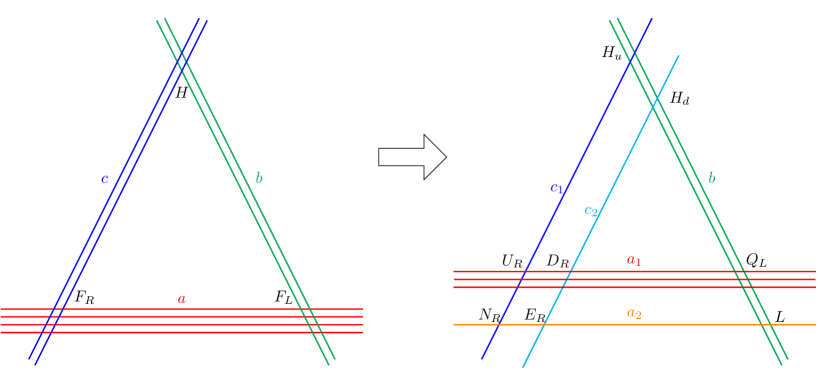
Refer to caption
Figure 1: Pati-Salam gauge group SU(4)×SU(2)L×SU(2)RSU4SUsubscript2𝐿SUsubscript2𝑅{\rm SU}(4)\times{\rm SU}(2)_{L}\times{\rm SU}(2)_{R} is broken down to the standard model gauge group SU(3)C×U(2)L×U(1)I3R×U(1)BLSUsubscript3𝐶Usubscript2𝐿Usubscript1𝐼3𝑅Usubscript1𝐵𝐿{\rm SU}(3)_{C}\times{\rm U}(2)_{L}\times{\rm U}(1)_{I3R}\times{\rm U}(1)_{B-L} via the process of brane splitting that corresponds to assigning VEVs to the adjoint scalars, which arise as open-string moduli associated with the positions of stacks a𝑎a and c𝑐c in the internal space.

Pati-Salam gauge group SU(4)×SU(2)L×SU(2)RSU4SUsubscript2𝐿SUsubscript2𝑅{\rm SU}(4)\times{\rm SU}(2)_{L}\times{\rm SU}(2)_{R} is higgsed down to the standard model gauge group SU(3)C×U(2)L×U(1)I3R×U(1)BLSUsubscript3𝐶Usubscript2𝐿Usubscript1𝐼3𝑅Usubscript1𝐵𝐿{\rm SU}(3)_{C}\times{\rm U}(2)_{L}\times{\rm U}(1)_{I3R}\times{\rm U}(1)_{B-L} by assigning vacuum expectation values to the adjoint scalars which arise as open-string moduli associated to the stacks a𝑎a and c𝑐c, see figure 1,

a𝑎\displaystyle{\color[rgb]{1,0,0}a} \displaystyle\rightarrow a1+a2,subscript𝑎1subscript𝑎2\displaystyle{\color[rgb]{1,0,0}a_{1}}+{\color[rgb]{1,.5,0}a_{2}},
c𝑐\displaystyle{\color[rgb]{0,0,1}c} \displaystyle\rightarrow c1+c2.subscript𝑐1subscript𝑐2\displaystyle{\color[rgb]{0,0,1}c_{1}}+{\color[rgb]{0,1,1}c_{2}}. (14)

Moreover, the U(1)I3R×U(1)BLUsubscript1subscript𝐼3𝑅Usubscript1𝐵𝐿{\rm U}(1)_{I_{3R}}\times{\rm U}(1)_{B-L} gauge symmetry may be broken to U(1)YUsubscript1𝑌{\rm U}(1)_{Y} by giving vacuum expectation values (VEVs) to the vector-like particles with the quantum numbers (𝟏,𝟏,𝟏/𝟐,𝟏)11121({\bf{1},1,1/2,-1}) and (𝟏,𝟏,𝟏/𝟐,𝟏)11121({\bf{1},1,-1/2,1}) under the SU(3)C×SU(2)L×U(1)I3R×U(1)BLSUsubscript3𝐶SUsubscript2𝐿Usubscript1subscript𝐼3𝑅Usubscript1𝐵𝐿{\rm SU}(3)_{C}\times{\rm SU}(2)_{L}\times{\rm U}(1)_{I_{3R}}\times{\rm U}(1)_{B-L} gauge symmetry from a2c1subscript𝑎2superscriptsubscript𝑐1a_{2}c_{1}^{\prime} intersections Cvetic:2004ui ; Chen:2006gd .

This brane-splitting results in standard model quarks and leptons as Cvetic:2004nk ,

FL(QL,LL)subscript𝐹𝐿subscript𝑄𝐿subscript𝐿𝐿\displaystyle F_{L}(Q_{L},L_{L}) \displaystyle\rightarrow QL+L,subscript𝑄𝐿𝐿\displaystyle Q_{L}+L,
FR(QR,LR)subscript𝐹𝑅subscript𝑄𝑅subscript𝐿𝑅\displaystyle F_{R}(Q_{R},L_{R}) \displaystyle\rightarrow UR+DR+ER+N.subscript𝑈𝑅subscript𝐷𝑅subscript𝐸𝑅𝑁\displaystyle U_{R}+D_{R}+E_{R}+N. (15)

Three-point Yukawa couplings for the quarks and the charged leptons can be read from the following superpotential,

𝒲3YijkuQiUjcHku+YijkdQiDjcHkd+YijkνLiNjcHku+YijkeLiEjcHkd,similar-tosubscript𝒲3subscriptsuperscript𝑌𝑢𝑖𝑗𝑘subscript𝑄𝑖subscriptsuperscript𝑈𝑐𝑗subscriptsuperscript𝐻𝑢𝑘subscriptsuperscript𝑌𝑑𝑖𝑗𝑘subscript𝑄𝑖subscriptsuperscript𝐷𝑐𝑗subscriptsuperscript𝐻𝑑𝑘subscriptsuperscript𝑌𝜈𝑖𝑗𝑘subscript𝐿𝑖subscriptsuperscript𝑁𝑐𝑗subscriptsuperscript𝐻𝑢𝑘subscriptsuperscript𝑌𝑒𝑖𝑗𝑘subscript𝐿𝑖subscriptsuperscript𝐸𝑐𝑗subscriptsuperscript𝐻𝑑𝑘\displaystyle\mathcal{W}_{3}\sim Y^{u}_{ijk}Q_{i}U^{c}_{j}H^{u}_{k}+Y^{d}_{ijk}Q_{i}D^{c}_{j}H^{d}_{k}+Y^{\nu}_{ijk}L_{i}N^{c}_{j}H^{u}_{k}+Y^{e}_{ijk}L_{i}E^{c}_{j}H^{d}_{k}, (16)

where Yijkusubscriptsuperscript𝑌𝑢𝑖𝑗𝑘Y^{u}_{ijk}, Yijkdsubscriptsuperscript𝑌𝑑𝑖𝑗𝑘Y^{d}_{ijk}, Yijkνsubscriptsuperscript𝑌𝜈𝑖𝑗𝑘Y^{\nu}_{ijk} and Yijkesubscriptsuperscript𝑌𝑒𝑖𝑗𝑘Y^{e}_{ijk} are Yukawa couplings, and Qisubscript𝑄𝑖Q_{i}, Uicsubscriptsuperscript𝑈𝑐𝑖U^{c}_{i}, Dicsubscriptsuperscript𝐷𝑐𝑖D^{c}_{i}, Lisubscript𝐿𝑖L_{i}, Nicsubscriptsuperscript𝑁𝑐𝑖N^{c}_{i}, and Eicsubscriptsuperscript𝐸𝑐𝑖E^{c}_{i} are the left-handed quark doublet, right-handed up-type quarks, right-handed down-type quarks, left-handed lepton doublet, right-handed neutrinos, and right-handed leptons, respectively. The superpotential including the four-point interactions is

𝒲41MS(YijkluQiUjcHkuSlL+YijkldQiDjcHkdSlL+YijklνLiNjcHkuSlL+YijkleLiEjcHkdSlL),similar-tosubscript𝒲41subscript𝑀Ssubscriptsuperscript𝑌𝑢𝑖𝑗𝑘𝑙subscript𝑄𝑖subscriptsuperscript𝑈𝑐𝑗subscriptsuperscript𝐻𝑢𝑘subscriptsuperscript𝑆𝐿𝑙subscriptsuperscript𝑌𝑑𝑖𝑗𝑘𝑙subscript𝑄𝑖subscriptsuperscript𝐷𝑐𝑗subscriptsuperscript𝐻𝑑𝑘subscriptsuperscript𝑆𝐿𝑙subscriptsuperscript𝑌𝜈𝑖𝑗𝑘𝑙subscript𝐿𝑖subscriptsuperscript𝑁𝑐𝑗subscriptsuperscript𝐻𝑢𝑘subscriptsuperscript𝑆𝐿𝑙subscriptsuperscript𝑌𝑒𝑖𝑗𝑘𝑙subscript𝐿𝑖subscriptsuperscript𝐸𝑐𝑗subscriptsuperscript𝐻𝑑𝑘subscriptsuperscript𝑆𝐿𝑙\displaystyle\mathcal{W}_{4}\sim{1\over{M_{\rm S}}}\left(Y^{\prime u}_{ijkl}Q_{i}U^{c}_{j}H^{\prime u}_{k}S^{L}_{l}+Y^{\prime d}_{ijkl}Q_{i}D^{c}_{j}H^{\prime d}_{k}S^{L}_{l}+Y^{\prime\nu}_{ijkl}L_{i}N^{c}_{j}H^{\prime u}_{k}S^{L}_{l}+Y^{\prime e}_{ijkl}L_{i}E^{c}_{j}H^{\prime d}_{k}S^{L}_{l}\right), (17)

where Yijklusubscriptsuperscript𝑌𝑢𝑖𝑗𝑘𝑙Y^{\prime u}_{ijkl}, Yijkldsubscriptsuperscript𝑌𝑑𝑖𝑗𝑘𝑙Y^{\prime d}_{ijkl}, Yijklνsubscriptsuperscript𝑌𝜈𝑖𝑗𝑘𝑙Y^{\prime\nu}_{ijkl}, and Yijklesubscriptsuperscript𝑌𝑒𝑖𝑗𝑘𝑙Y^{\prime e}_{ijkl} are Yukawa couplings of the four-point functions, and MSsubscript𝑀SM_{\rm S} is the string scale.

The additional exotic particles must be made superheavy to ensure gauge coupling unification at the string scale. Similar to Refs. Cvetic:2007ku ; Chen:2007zu we can decouple the additional exotic particles except the charged chiral multiplets under SU(4)CSUsubscript4𝐶{\rm SU}(4)_{C} anti-symmetric representation. These chiral multiplets can be decoupled via instanton effects in principle Blumenhagen:2006xt ; Haack:2006cy ; Florea:2006si .

We now turn our attention toward the four dimensional low energy effective field theory. 𝒩=1𝒩1\mathcal{N}=1 supergravity action is encoded by three functions viz. the gauge kinetic function fxsubscript𝑓𝑥f_{x}, the Kähler potential K𝐾K and the superpotential W𝑊W Cremmer:1982en . Each of these functions in turn depend on dilaton S𝑆S, complex T𝑇T, and Kähler U𝑈U moduli.

The complex structure moduli Uisuperscript𝑈𝑖U^{i} can be obtained as,

Ujsuperscript𝑈𝑗\displaystyle U^{j} =4iχj+2βjχj24+βjχj2,χjR2jR1j.\displaystyle=\frac{4i\chi^{j}+2\beta_{j}\chi_{j}^{2}}{4+\beta_{j}\chi_{j}^{2}},\qquad\because\chi^{j}\equiv\frac{R_{2}^{j}}{R_{1}^{j}}. (18)

These upper case moduli in string theory basis can be transformed in to lower case s𝑠s, t𝑡t, u𝑢u moduli in field theory basis as Lust:2004cx ,

Re(s)Re𝑠\displaystyle\mathrm{Re}\,(s) =eϕ42π(ImU1ImU2ImU3|U1U2U3|),absentsuperscript𝑒subscriptitalic-ϕ42𝜋Imsuperscript𝑈1Imsuperscript𝑈2Imsuperscript𝑈3superscript𝑈1superscript𝑈2superscript𝑈3\displaystyle=\frac{e^{-{\phi}_{4}}}{2\pi}\,\left(\frac{\sqrt{\mathrm{Im}\,U^{1}\,\mathrm{Im}\,U^{2}\,\mathrm{Im}\,U^{3}}}{|U^{1}U^{2}U^{3}|}\right),
Re(uj)Resuperscript𝑢𝑗\displaystyle\mathrm{Re}\,(u^{j}) =eϕ42π(ImUjImUkImUl)|UkUlUj|,(j,k,l)=(1,2,3¯),formulae-sequenceabsentsuperscript𝑒subscriptitalic-ϕ42𝜋Imsuperscript𝑈𝑗Imsuperscript𝑈𝑘Imsuperscript𝑈𝑙superscript𝑈𝑘superscript𝑈𝑙superscript𝑈𝑗𝑗𝑘𝑙¯123\displaystyle=\frac{e^{-{\phi}_{4}}}{2\pi}\left(\sqrt{\frac{\mathrm{Im}\,U^{j}}{\mathrm{Im}\,U^{k}\,\mathrm{Im}\,U^{l}}}\right)\;\left|\frac{U^{k}\,U^{l}}{U^{j}}\right|,\quad(j,k,l)=(\overline{1,2,3}),
Re(tj)Resuperscript𝑡𝑗\displaystyle\mathrm{Re}(t^{j}) =iαTj,absent𝑖superscript𝛼superscript𝑇𝑗\displaystyle=\frac{i\alpha^{\prime}}{T^{j}}, (19)

where j𝑗j denotes the jthsuperscript𝑗thj^{\rm th} two-torus, and ϕ4subscriptitalic-ϕ4\phi_{4} is the four dimensional dilaton which is related to the supergravity moduli as

2πeϕ4=(Re(s)Re(u1)Re(u2)Re(u3))1/4.2𝜋superscript𝑒subscriptitalic-ϕ4superscriptRe𝑠Resubscript𝑢1Resubscript𝑢2Resubscript𝑢3142\pi e^{\phi_{4}}=\Big{(}\mathrm{Re}(s)\,\mathrm{Re}(u_{1})\,\mathrm{Re}(u_{2})\,\mathrm{Re}(u_{3})\Big{)}^{-1/4}. (20)

Inverting the above formulas we can solve for U𝑈U moduli in string theory basis in terms of s𝑠s and u𝑢u as,

|Uj|2Im(Uj)=Re(uk)Re(ul)Re(uj)Re(s),(j,k,l)=(1,2,3¯).formulae-sequencesuperscriptsuperscript𝑈𝑗2Imsuperscript𝑈𝑗Resuperscript𝑢𝑘Resuperscript𝑢𝑙Resuperscript𝑢𝑗Re𝑠𝑗𝑘𝑙¯123\frac{|U^{j}|^{2}}{\mathrm{Im}\,(U^{j})}=\sqrt{\frac{\mathrm{Re}\,(u^{k})\,\mathrm{Re}\,(u^{l})}{\mathrm{Re}\,(u^{j})\mathrm{Re}\,(s)}},\quad(j,k,l)=(\overline{1,2,3}). (21)

The holomorphic gauge kinetic function for any D6-brane stack x𝑥x wrapping a calibrated 3-cycle is given as Blumenhagen:2006ci ,

fx=12πs3[eϕΠxRe(eiθxΩ3)iΠxC3],subscript𝑓𝑥12𝜋superscriptsubscript𝑠3delimited-[]superscript𝑒italic-ϕsubscriptsubscriptΠ𝑥Resuperscript𝑒𝑖subscript𝜃𝑥subscriptΩ3𝑖subscriptsubscriptΠ𝑥subscript𝐶3f_{x}=\frac{1}{2\pi\ell_{s}^{3}}\left[e^{-\phi}\int_{\Pi_{x}}\mathrm{Re}(e^{-i\theta_{x}}\Omega_{3})-i\int_{\Pi_{x}}C_{3}\right], (22)

where the integral involving 3-form Ω3subscriptΩ3\Omega_{3} gives,

ΠxΩ3=14i=13(nxiR1i+2βiilxiR2i).subscriptsubscriptΠ𝑥subscriptΩ314superscriptsubscriptproduct𝑖13superscriptsubscript𝑛𝑥𝑖superscriptsubscript𝑅1𝑖superscript2subscript𝛽𝑖𝑖superscriptsubscript𝑙𝑥𝑖superscriptsubscript𝑅2𝑖\int_{\Pi_{x}}\Omega_{3}=\frac{1}{4}\prod_{i=1}^{3}(n_{x}^{i}R_{1}^{i}+2^{-\beta_{i}}il_{x}^{i}R_{2}^{i}). (23)

It can then be shown that,

fxsubscript𝑓𝑥\displaystyle f_{x} =14κx(nx1nx2nx3snx1lx2lx3u12(β2+β3)lx1nx2lx3u22(β1+β3)lx1lx2nx3u32(β1+β2)),absent14subscript𝜅𝑥superscriptsubscript𝑛𝑥1superscriptsubscript𝑛𝑥2superscriptsubscript𝑛𝑥3𝑠superscriptsubscript𝑛𝑥1superscriptsubscript𝑙𝑥2superscriptsubscript𝑙𝑥3superscript𝑢1superscript2subscript𝛽2subscript𝛽3superscriptsubscript𝑙𝑥1superscriptsubscript𝑛𝑥2superscriptsubscript𝑙𝑥3superscript𝑢2superscript2subscript𝛽1subscript𝛽3superscriptsubscript𝑙𝑥1superscriptsubscript𝑙𝑥2superscriptsubscript𝑛𝑥3superscript𝑢3superscript2subscript𝛽1subscript𝛽2\displaystyle=\frac{1}{4\kappa_{x}}(n_{x}^{1}\,n_{x}^{2}\,n_{x}^{3}\,s-\frac{n_{x}^{1}\,l_{x}^{2}\,l_{x}^{3}\,u^{1}}{2^{(\beta_{2}+\beta_{3})}}-\frac{l_{x}^{1}\,n_{x}^{2}\,l_{x}^{3}\,u^{2}}{2^{(\beta_{1}+\beta_{3})}}-\frac{l_{x}^{1}\,l_{x}^{2}\,n_{x}^{3}\,u^{3}}{2^{(\beta_{1}+\beta_{2})}}), (24)

where the factor κxsubscript𝜅𝑥{\kappa}_{x} is related to the difference between the gauge couplings for U(Nx)Usubscript𝑁𝑥{\rm U}(N_{x}) and Sp(2Nx),SO(2Nx)𝑆𝑝2subscript𝑁𝑥𝑆𝑂2subscript𝑁𝑥Sp(2N_{x}),\,SO(2N_{x}). κx=1subscript𝜅𝑥1{\kappa}_{x}=1 for U(Nx)Usubscript𝑁𝑥{\rm U}(N_{x}) and κx=2subscript𝜅𝑥2{\kappa}_{x}=2 for Sp(2Nx)𝑆𝑝2subscript𝑁𝑥Sp(2N_{x}) or SO(2Nx)𝑆𝑂2subscript𝑁𝑥SO(2N_{x}) Klebanov:2003my . Since, the standard model hypercharge U(1)YUsubscript1𝑌{\rm U}(1)_{Y} is a linear combination of several U(1)U1{\rm U}(1)s,

QY=16Qa1+12Qa212Qc112Qc2.subscript𝑄𝑌16subscript𝑄subscript𝑎112subscript𝑄subscript𝑎212subscript𝑄subscript𝑐112subscript𝑄subscript𝑐2Q_{Y}=\frac{1}{6}Q_{a_{1}}+\frac{1}{2}Q_{a_{2}}-\frac{1}{2}Q_{c_{1}}-\frac{1}{2}Q_{c_{2}}. (25)

Therefore, the holomorphic gauge kinetic function for the hypercharge is also taken as a linear combination of the kinetic gauge functions from all of the stacks as Blumenhagen:2003jy ; Ibanez:2001nd ,

fY=16fa1+12fa2+12fc1+12fc2.subscript𝑓𝑌16subscript𝑓subscript𝑎112subscript𝑓subscript𝑎212subscript𝑓subscript𝑐112subscript𝑓subscript𝑐2f_{Y}=\frac{1}{6}f_{a_{1}}+\frac{1}{2}f_{a_{2}}+\frac{1}{2}f_{c_{1}}+\frac{1}{2}f_{c_{2}}. (26)

The Kähler potential to the second order for the moduli M𝑀M and open string matter fields Ci,Cθsubscript𝐶𝑖subscript𝐶𝜃C_{i},C_{\theta} is given by :

K(M,M¯,C,C¯)𝐾𝑀¯𝑀𝐶¯𝐶\displaystyle K(M,\bar{M},C,\bar{C}) =K^(M,M¯)+untwistedi,jK~CiC¯j(M,M¯)CiC¯jabsent^𝐾𝑀¯𝑀subscriptuntwisted𝑖𝑗subscript~𝐾subscript𝐶𝑖subscript¯𝐶𝑗𝑀¯𝑀subscript𝐶𝑖subscript¯𝐶𝑗\displaystyle=\hat{K}(M,\bar{M})+\sum_{\mathrm{untwisted}\,i,j}\tilde{K}_{C_{i}\bar{C}_{j}}(M,\bar{M})C_{i}\bar{C}_{j}
+twisted,θK~CθC¯θ(M,M¯)CθC¯θ,subscripttwisted𝜃subscript~𝐾subscript𝐶𝜃subscript¯𝐶𝜃𝑀¯𝑀subscript𝐶𝜃subscript¯𝐶𝜃\displaystyle\quad+\sum_{\mathrm{twisted},\,\theta}\tilde{K}_{C_{\theta}\bar{C}_{\theta}}(M,\bar{M})C_{\theta}\bar{C}_{\theta}, (27)

where Cisubscript𝐶𝑖C_{i} correspond to the D-brane positions and the Wilson lines moduli arising from strings having both ends on the same stack while Cθsubscript𝐶𝜃C_{\theta} correspond to strings stretching between different stacks comprising 1/4141/4 BPS branes. The untwisted moduli fields Ci,C¯jsubscript𝐶𝑖subscript¯𝐶𝑗C_{i},\bar{C}_{j} are not present in MSSM and must become heavy via higher dimensional operators111D-branes wrapping rigid cycles can freeze such open string moduli Blumenhagen:2005tn , however such rigid cycles without discrete torsion are not present in 𝐓6/(2×2)superscript𝐓6subscript2subscript2\mathbf{T}^{6}/(\mathbb{Z}_{2}\times\mathbb{Z}_{2})..

Let us determine the Kähler metric K~CθC¯θ(M,M¯)subscript~𝐾subscript𝐶𝜃subscript¯𝐶𝜃𝑀¯𝑀\tilde{K}_{C_{\theta}\bar{C}_{\theta}}(M,\bar{M}) for the twisted moduli. We denote the Kähler potential arising from strings stretching between stacks x𝑥x and y𝑦y as K~xysubscript~𝐾𝑥𝑦\tilde{K}_{xy} and θxyjθyjθxjsubscriptsuperscript𝜃𝑗𝑥𝑦subscriptsuperscript𝜃𝑗𝑦subscriptsuperscript𝜃𝑗𝑥\theta^{j}_{xy}\equiv\theta^{j}_{y}-\theta^{j}_{x} denotes the angle between the cycles wrapped by the branes x𝑥x and y𝑦y on the jthsuperscript𝑗thj^{\rm th} two-torus with the constraint jθxyj=0subscript𝑗subscriptsuperscript𝜃𝑗𝑥𝑦0\sum_{j}\theta^{j}_{xy}=0. Following Font:2004cx ; Cvetic:2003ch ; Lust:2004cx , we find two cases for the Kähler metric in type IIA theory:

  • θxyj<0subscriptsuperscript𝜃𝑗𝑥𝑦0\theta^{j}_{xy}<0, θxyk>0subscriptsuperscript𝜃𝑘𝑥𝑦0\theta^{k}_{xy}>0, θxyl>0subscriptsuperscript𝜃𝑙𝑥𝑦0\theta^{l}_{xy}>0

    K~xysubscript~𝐾𝑥𝑦\displaystyle\tilde{K}_{xy} =eϕ4eγE(2j=13θxyj)Γ(θxyj)Γ(1+θxyj)Γ(1θxyk)Γ(θxyk)Γ(1θxyl)Γ(θxyl)absentsuperscript𝑒subscriptitalic-ϕ4superscript𝑒subscript𝛾𝐸2superscriptsubscript𝑗13subscriptsuperscript𝜃𝑗𝑥𝑦Γsubscriptsuperscript𝜃𝑗𝑥𝑦Γ1subscriptsuperscript𝜃𝑗𝑥𝑦Γ1subscriptsuperscript𝜃𝑘𝑥𝑦Γsubscriptsuperscript𝜃𝑘𝑥𝑦Γ1subscriptsuperscript𝜃𝑙𝑥𝑦Γsubscriptsuperscript𝜃𝑙𝑥𝑦\displaystyle=e^{\phi_{4}}e^{\gamma_{E}(2-\sum_{j=1}^{3}\theta^{j}_{xy})}\sqrt{\frac{\Gamma(\theta^{j}_{xy})}{\Gamma(1+\theta^{j}_{xy})}}\sqrt{\frac{\Gamma(1-\theta^{k}_{xy})}{\Gamma(\theta^{k}_{xy})}}\sqrt{\frac{\Gamma(1-\theta^{l}_{xy})}{\Gamma(\theta^{l}_{xy})}}
    (tj+t¯j)θxyj(tk+t¯k)1+θxyk(tl+t¯l)1+θxyl.superscriptsuperscript𝑡𝑗superscript¯𝑡𝑗subscriptsuperscript𝜃𝑗𝑥𝑦superscriptsuperscript𝑡𝑘superscript¯𝑡𝑘1subscriptsuperscript𝜃𝑘𝑥𝑦superscriptsuperscript𝑡𝑙superscript¯𝑡𝑙1subscriptsuperscript𝜃𝑙𝑥𝑦\displaystyle\quad(t^{j}+\bar{t}^{j})^{\theta^{j}_{xy}}(t^{k}+\bar{t}^{k})^{-1+\theta^{k}_{xy}}(t^{l}+\bar{t}^{l})^{-1+\theta^{l}_{xy}}. (28)
  • θxyj<0subscriptsuperscript𝜃𝑗𝑥𝑦0\theta^{j}_{xy}<0, θxyk<0subscriptsuperscript𝜃𝑘𝑥𝑦0\theta^{k}_{xy}<0, θxyl>0subscriptsuperscript𝜃𝑙𝑥𝑦0\theta^{l}_{xy}>0

    K~xysubscript~𝐾𝑥𝑦\displaystyle\tilde{K}_{xy} =eϕ4eγE(2+j=13θxyj)Γ(1+θxyj)Γ(θxyj)Γ(1+θxyk)Γ(θxyk)Γ(θxyl)Γ(1θxyl)absentsuperscript𝑒subscriptitalic-ϕ4superscript𝑒subscript𝛾𝐸2superscriptsubscript𝑗13subscriptsuperscript𝜃𝑗𝑥𝑦Γ1subscriptsuperscript𝜃𝑗𝑥𝑦Γsubscriptsuperscript𝜃𝑗𝑥𝑦Γ1subscriptsuperscript𝜃𝑘𝑥𝑦Γsubscriptsuperscript𝜃𝑘𝑥𝑦Γsubscriptsuperscript𝜃𝑙𝑥𝑦Γ1subscriptsuperscript𝜃𝑙𝑥𝑦\displaystyle=e^{\phi_{4}}e^{\gamma_{E}(2+\sum_{j=1}^{3}\theta^{j}_{xy})}\sqrt{\frac{\Gamma(1+\theta^{j}_{xy})}{\Gamma(-\theta^{j}_{xy})}}\sqrt{\frac{\Gamma(1+\theta^{k}_{xy})}{\Gamma(-\theta^{k}_{xy})}}\sqrt{\frac{\Gamma(\theta^{l}_{xy})}{\Gamma(1-\theta^{l}_{xy})}}
    (tj+t¯j)1θxyj(tk+t¯k)1θxyk(tl+t¯l)θxyl.superscriptsuperscript𝑡𝑗superscript¯𝑡𝑗1subscriptsuperscript𝜃𝑗𝑥𝑦superscriptsuperscript𝑡𝑘superscript¯𝑡𝑘1subscriptsuperscript𝜃𝑘𝑥𝑦superscriptsuperscript𝑡𝑙superscript¯𝑡𝑙subscriptsuperscript𝜃𝑙𝑥𝑦\displaystyle\quad(t^{j}+\bar{t}^{j})^{-1-\theta^{j}_{xy}}(t^{k}+\bar{t}^{k})^{-1-\theta^{k}_{xy}}(t^{l}+\bar{t}^{l})^{-\theta^{l}_{xy}}. (29)

The Kähler metric for the branes parallel to at least one torus which give rise to non-chiral matter in bifundamental representations (1/2 BPS scalar) like the Higgs doublet is,

K^higgs=[(s+s¯)(t1+t¯1)(t2+t¯2)(u3+u¯3)]1/2.subscript^𝐾higgssuperscriptdelimited-[]𝑠¯𝑠superscript𝑡1superscript¯𝑡1superscript𝑡2superscript¯𝑡2superscript𝑢3superscript¯𝑢312\hat{K}_{\mathrm{higgs}}=\left[(s+\bar{s})(t^{1}+\bar{t}^{1})(t^{2}+\bar{t}^{2})(u^{3}+\bar{u}^{3})\right]^{-1/2}. (30)

The superpotential is given as,

W=W^+12μαβ(M)CαCβ+16Yαβγ(M)CαCβCγ+𝑊^𝑊12subscript𝜇𝛼𝛽𝑀superscript𝐶𝛼superscript𝐶𝛽16subscript𝑌𝛼𝛽𝛾𝑀superscript𝐶𝛼superscript𝐶𝛽superscript𝐶𝛾W=\hat{W}+\frac{1}{2}{\mu}_{\alpha\beta}(M)\,C^{\alpha}\,C^{\beta}+\frac{1}{6}\,Y_{\alpha\beta\gamma}(M)\,C^{\alpha}\,C^{\beta}\,C^{\gamma}+... (31)

and the minimum of the tree-level F-term supergravity scalar potential is given by222In our analysis we assume that D-terms do not affect the soft terms Kawamura:1996ex ; Komargodski:2009pc .

V(M,M¯)𝑉𝑀¯𝑀\displaystyle V(M,\bar{M}) =eG(GMKMNGN3)absentsuperscript𝑒𝐺subscript𝐺𝑀superscript𝐾𝑀𝑁subscript𝐺𝑁3\displaystyle=e^{G}(G_{M}K^{MN}G_{N}-3)
=(FMKMNFN3eG),absentsuperscript𝐹𝑀subscript𝐾𝑀𝑁superscript𝐹𝑁3superscript𝑒𝐺\displaystyle=(F^{M}K_{MN}F^{N}-3e^{G}), (32)

where GM=MGsubscript𝐺𝑀subscript𝑀𝐺G_{M}=\partial_{M}G, KMN=MNKsubscript𝐾𝑀𝑁subscript𝑀subscript𝑁𝐾K_{MN}=\partial_{M}\partial_{N}K, KMNsuperscript𝐾𝑀𝑁K^{MN} is the inverse Kähler metric, and the auxiliary fields FMsuperscript𝐹𝑀F^{M} are,

FM=eG/2KMNGN.superscript𝐹𝑀superscript𝑒𝐺2superscript𝐾𝑀𝑁subscript𝐺𝑁F^{M}=e^{G/2}K^{MN}G_{N}. (33)

Thus supersymmetry is broken via F-terms from some of the hidden sector fields M𝑀M acquiring VEVs, thereby generating soft terms in the observable sector Font:2004cx ; Kane:2004hm ; Chen:2007zu . Gravitino gets massive by absorbing goldstino via the superhiggs mechanism.

m3/2=eG/2.subscript𝑚32superscript𝑒𝐺2m_{3/2}=e^{G/2}. (34)

The normalized soft parameters viz. the gaugino mass, squared scalar mass and trilinear parameters are given by Brignole:1997dp ,

Mxsubscript𝑀𝑥\displaystyle M_{x} =12Refx(FMMfx),absent12Resubscript𝑓𝑥superscript𝐹𝑀subscript𝑀subscript𝑓𝑥\displaystyle=\frac{1}{2\,\mathrm{Re}\,f_{x}}\,(F^{M}\,\partial_{M}\,f_{x}),
mxy2superscriptsubscript𝑚𝑥𝑦2\displaystyle m_{xy}^{2} =(m3/22+V0)M,NF¯M¯FNM¯Nlog(K~xy),absentsuperscriptsubscript𝑚322subscript𝑉0subscript𝑀𝑁superscript¯𝐹¯𝑀superscript𝐹𝑁subscript¯𝑀subscript𝑁subscript~𝐾𝑥𝑦\displaystyle=(m_{3/2}^{2}+V_{0})-\sum_{M,N}\,\bar{F}^{\bar{M}}F^{N}\,{\partial}_{\bar{M}}\,{\partial}_{N}\,\log({\tilde{K}}_{xy}),
Axyzsubscript𝐴𝑥𝑦𝑧\displaystyle A_{xyz} =FM[K^M+Mlog(Yxyz)Mlog(K~xyK~yzK~zx)],absentsuperscript𝐹𝑀delimited-[]subscript^𝐾𝑀subscript𝑀subscript𝑌𝑥𝑦𝑧subscript𝑀subscript~𝐾𝑥𝑦subscript~𝐾𝑦𝑧subscript~𝐾𝑧𝑥\displaystyle=F^{M}[\hat{K}_{M}+{\partial}_{M}\,\log(Y_{xyz})-{\partial}_{M}\,\log(\tilde{K}_{xy}\tilde{K}_{yz}\tilde{K}_{zx})], (35)

where K^Msubscript^𝐾𝑀\hat{K}_{M} is the Kähler metric for branes parallel to at least one torus and FMsuperscript𝐹𝑀F^{M} denotes auxiliary fields.

Although it appears that soft terms may depend on the Yukawa couplings via the superpotential, however these are not the physical Yukawa couplings which exponentially depend on the worldsheet area. Both are related by the following relation,

Yxyzphys=YxyzW^|W^|eK^/2(K~xK~yK~z)1/2.subscriptsuperscript𝑌phys𝑥𝑦𝑧subscript𝑌𝑥𝑦𝑧superscript^𝑊^𝑊superscript𝑒^𝐾2superscriptsubscript~𝐾𝑥subscript~𝐾𝑦subscript~𝐾𝑧12Y^{\mathrm{phys}}_{xyz}=Y_{xyz}\,\frac{\hat{W}^{*}}{|\hat{W}|}\,e^{\hat{K}/2}\,(\tilde{K}_{x}\tilde{K}_{y}\tilde{K}_{z})^{-1/2}. (36)

To calculate the soft terms from supersymmetry breaking we ignore the cosmological constant V0subscript𝑉0V_{0} and introduce the following VEVs for the auxiliary fields (33) for the s𝑠s, t𝑡t and u𝑢u moduli Brignole:1993dj ,

Fssuperscript𝐹𝑠\displaystyle F^{s} =23Cm3/2Re(s)Θseiγs,absent23𝐶subscript𝑚32Re𝑠subscriptΘ𝑠superscript𝑒𝑖subscript𝛾𝑠\displaystyle=2\sqrt{3}Cm_{3/2}\mathrm{Re}(s)\Theta_{s}e^{-i\gamma_{s}},
F{u,t}isuperscript𝐹superscript𝑢𝑡𝑖\displaystyle F^{\{u,t\}^{i}} =23Cm3/2(Re(ui)Θiueiγiu+Re(ti)Θiteiγit),absent23𝐶subscript𝑚32Resuperscript𝑢𝑖superscriptsubscriptΘ𝑖𝑢superscript𝑒𝑖subscriptsuperscript𝛾𝑢𝑖Resuperscript𝑡𝑖superscriptsubscriptΘ𝑖𝑡superscript𝑒𝑖superscriptsubscript𝛾𝑖𝑡\displaystyle=2\sqrt{3}Cm_{3/2}\left(\mathrm{Re}({u}^{i})\Theta_{i}^{u}e^{-i\gamma^{u}_{i}}+\mathrm{Re}({t}^{i})\Theta_{i}^{t}e^{-i\gamma_{i}^{t}}\right), (37)

Here, the factors γssubscript𝛾𝑠\gamma_{s} and γisubscript𝛾𝑖\gamma_{i} denote the CP violating phases of the moduli. The constant C𝐶C is given by the gravitino-mass m3/22subscriptsuperscript𝑚232m^{2}_{3/2} and the cosmological constant V0subscript𝑉0V_{0} as C2=1+V03m3/22superscript𝐶21subscript𝑉03subscriptsuperscript𝑚232C^{2}=1+\frac{V_{0}}{3m^{2}_{3/2}}. ΘssubscriptΘ𝑠\Theta_{s} and Θit,usubscriptsuperscriptΘ𝑡𝑢𝑖\Theta^{t,u}_{i} are the goldstino angles which determine the degree to which supersymmetry breaking is being dominated by any of the dilaton s𝑠s, complex structure (uisuperscript𝑢𝑖u^{i}) and Kähler (tisuperscript𝑡𝑖t^{i}) moduli constrained by the relation,

i=13(|Θiu|2+|Θit|2)+|Θs|2=1.superscriptsubscript𝑖13superscriptsuperscriptsubscriptΘ𝑖𝑢2superscriptsuperscriptsubscriptΘ𝑖𝑡2superscriptsubscriptΘ𝑠21\displaystyle\sum_{i=1}^{3}(|\Theta_{i}^{u}|^{2}+|\Theta_{i}^{t}|^{2})+|\Theta_{s}|^{2}=1. (38)

Unlike the s𝑠s- or u𝑢u-moduli dominant supersymmetry breaking, the case of t𝑡t-moduli dominant susy breaking depends on the physical Yukawa couplings via the area of the triangles. Accordingly we shall concentrate on the general scenario with the u𝑢u-moduli dominated supersymmetry breaking with dilaton-modulus s𝑠s turned on, Fs0superscript𝐹𝑠0F^{s}\neq 0. We set the cosmological constant, V0subscript𝑉0V_{0} to be zero.

3.1 Supersymmetry breaking via u𝑢u-moduli and dilaton s𝑠s

Supersymmetry breaking via u𝑢u-moduli including a non-zero VEV for the dilaton s𝑠s results in the following auxiliary fields (3),

Fs,ui=3m3/2[(s+s¯)Θseiγs+(ui+u¯i)Θieiγi].superscript𝐹𝑠superscript𝑢𝑖3subscript𝑚32delimited-[]𝑠¯𝑠subscriptΘ𝑠superscript𝑒𝑖subscript𝛾𝑠superscript𝑢𝑖superscript¯𝑢𝑖subscriptΘ𝑖superscript𝑒𝑖subscript𝛾𝑖F^{s,u^{i}}=\sqrt{3}m_{3/2}[(s+\bar{s})\Theta_{s}e^{-i\gamma_{s}}+(u^{i}+\bar{u}^{i})\Theta_{i}e^{-i\gamma_{i}}]. (39)

To calculate the soft terms, we need to know the derivatives of the Kähler potential with respect to u𝑢u. Defining K~xyeϕ4K~xy0subscript~𝐾𝑥𝑦superscript𝑒subscriptitalic-ϕ4subscriptsuperscript~𝐾0𝑥𝑦\tilde{K}_{xy}\equiv e^{{\phi}_{4}}\,\tilde{K}^{0}_{xy} and using (28) and (29), we compute the derivatives with respect to uisuperscript𝑢𝑖u^{i} as,

logK~xyuisubscript~𝐾𝑥𝑦superscript𝑢𝑖\displaystyle\frac{\partial\log{\tilde{K}_{xy}}}{\partial u^{i}} =j=13logK~xy0θxyjθxyjui14(ui+u¯i),absentsuperscriptsubscript𝑗13subscriptsuperscript~𝐾0𝑥𝑦subscriptsuperscript𝜃𝑗𝑥𝑦subscriptsuperscript𝜃𝑗𝑥𝑦superscript𝑢𝑖14superscript𝑢𝑖superscript¯𝑢𝑖\displaystyle=\sum_{j=1}^{3}\frac{\partial\log{\tilde{K}^{0}_{xy}}}{\partial\theta^{j}_{xy}}\frac{\partial\theta^{j}_{xy}}{\partial u^{i}}-\frac{1}{4(u^{i}+\bar{u}^{i})}, (40)
2logK~xyui,¯ujsuperscript2subscript~𝐾𝑥𝑦superscript𝑢𝑖¯,superscript𝑢𝑗\displaystyle\frac{\partial^{2}\log{\tilde{K}_{xy}}}{\partial u^{i}\partial\bar{,}u^{j}} =k=13(logK~xy0θxyk2θxykuiu¯j+2logK~xy0(θxyk)2θxykuiθxyku¯j+δij4(ui+u¯i)2).absentsuperscriptsubscript𝑘13subscriptsuperscript~𝐾0𝑥𝑦subscriptsuperscript𝜃𝑘𝑥𝑦superscript2subscriptsuperscript𝜃𝑘𝑥𝑦superscript𝑢𝑖superscript¯𝑢𝑗superscript2subscriptsuperscript~𝐾0𝑥𝑦superscriptsubscriptsuperscript𝜃𝑘𝑥𝑦2subscriptsuperscript𝜃𝑘𝑥𝑦superscript𝑢𝑖subscriptsuperscript𝜃𝑘𝑥𝑦superscript¯𝑢𝑗subscript𝛿𝑖𝑗4superscriptsuperscript𝑢𝑖superscript¯𝑢𝑖2\displaystyle=\sum_{k=1}^{3}\left(\frac{\partial\log{\tilde{K}^{0}_{xy}}}{\partial\theta^{k}_{xy}}\frac{\partial^{2}\theta^{k}_{xy}}{\partial u^{i}\partial\bar{u}^{j}}+\frac{\partial^{2}\log\tilde{K}^{0}_{xy}}{\partial(\theta^{k}_{xy})^{2}}\frac{\partial\theta^{k}_{xy}}{\partial u^{i}}\frac{\partial\theta^{k}_{xy}}{\partial\bar{u}^{j}}+\frac{{\delta}_{ij}}{4\,(u^{i}+\bar{u}^{i})^{2}}\right). (41)

From the Kähler potential in (29), we have

Ψ(θxyj)Ψsubscriptsuperscript𝜃𝑗𝑥𝑦\displaystyle\Psi(\theta^{j}_{xy}) logK~xy0θxyj=γE+12ddθxyjlogΓ(1θxyj)12ddθxyjlogΓ(θxyj)log(tj+t¯j),absentsubscriptsuperscript~𝐾0𝑥𝑦subscriptsuperscript𝜃𝑗𝑥𝑦subscript𝛾𝐸12𝑑𝑑subscriptsuperscript𝜃𝑗𝑥𝑦Γ1subscriptsuperscript𝜃𝑗𝑥𝑦12𝑑𝑑subscriptsuperscript𝜃𝑗𝑥𝑦Γsubscriptsuperscript𝜃𝑗𝑥𝑦superscript𝑡𝑗superscript¯𝑡𝑗\displaystyle\equiv\frac{\partial\log{\tilde{K}^{0}_{xy}}}{\partial\theta^{j}_{xy}}=\gamma_{E}\!+\!\frac{1}{2}\frac{d}{d{\theta}^{j}_{xy}}\log{\Gamma(1-\theta^{j}_{xy})}-\frac{1}{2}\frac{d}{d{\theta}^{j}_{xy}}\log{\Gamma(\theta^{j}_{xy})}-\log(t^{j}+\bar{t}^{j}), (42)
Ψ(θxyj)superscriptΨsubscriptsuperscript𝜃𝑗𝑥𝑦\displaystyle\Psi^{\prime}(\theta^{j}_{xy}) 2logK~xy0(θxyj)2=dΨ(θxyj)dθxyj.absentsuperscript2subscriptsuperscript~𝐾0𝑥𝑦superscriptsubscriptsuperscript𝜃𝑗𝑥𝑦2𝑑Ψsubscriptsuperscript𝜃𝑗𝑥𝑦𝑑subscriptsuperscript𝜃𝑗𝑥𝑦\displaystyle\equiv\frac{\partial^{2}\log\tilde{K}^{0}_{xy}}{\partial(\theta^{j}_{xy})^{2}}=\frac{d\Psi(\theta^{j}_{xy})}{d\theta^{j}_{xy}}. (43)

The angles θxyjθyjθxjsubscriptsuperscript𝜃𝑗𝑥𝑦subscriptsuperscript𝜃𝑗𝑦subscriptsuperscript𝜃𝑗𝑥\theta^{j}_{xy}\equiv\theta^{j}_{y}-\theta^{j}_{x} are related to the u𝑢u moduli as,

tan(πθxj)=2βjlxjnxjReukReulReujReswhere(j,k,l)=(1,2,3¯).formulae-sequence𝜋subscriptsuperscript𝜃𝑗𝑥superscript2subscript𝛽𝑗subscriptsuperscript𝑙𝑗𝑥subscriptsuperscript𝑛𝑗𝑥Resuperscript𝑢𝑘Resuperscript𝑢𝑙Resuperscript𝑢𝑗Re𝑠where𝑗𝑘𝑙¯123\tan(\pi\theta^{j}_{x})=\frac{2^{-\beta_{j}}l^{j}_{x}}{n^{j}_{x}}\sqrt{\frac{\mathrm{Re}u^{k}\,\mathrm{Re}u^{l}}{\mathrm{Re}u^{j}\,\mathrm{Re}s}}\quad\mathrm{where~{}}(j,k,l)=(\overline{1,2,3}). (44)

And the first derivative of the angles are defined as,

θxyj,k(uk+u¯k)θxyjuk={[14πsin(2πθj)]yxwhenj=k[14πsin(2πθj)]yxwhenjksubscriptsuperscript𝜃𝑗𝑘𝑥𝑦superscript𝑢𝑘superscript¯𝑢𝑘subscriptsuperscript𝜃𝑗𝑥𝑦superscript𝑢𝑘casessubscriptsuperscriptdelimited-[]14𝜋2𝜋superscript𝜃𝑗𝑥𝑦when𝑗𝑘subscriptsuperscriptdelimited-[]14𝜋2𝜋superscript𝜃𝑗𝑥𝑦when𝑗𝑘{\theta}^{j,k}_{xy}\equiv(u^{k}+\bar{u}^{k})\,\frac{\partial\theta^{j}_{xy}}{\partial u^{k}}=\left\{\begin{array}[]{l}\left[-\frac{1}{4\pi}\sin(2\pi\theta^{j})\right]^{x}_{y}\quad\mathrm{when~{}}j=k\\ \left[\frac{1}{4\pi}\sin(2\pi\theta^{j})\right]^{x}_{y}\quad\mathrm{when~{}}j\neq k\end{array}\right. (45)
θxyj,s(s+s¯)θxyjs=14π[sin(2πθj)]yx,subscriptsuperscript𝜃𝑗𝑠𝑥𝑦𝑠¯𝑠subscriptsuperscript𝜃𝑗𝑥𝑦𝑠14𝜋subscriptsuperscriptdelimited-[]2𝜋superscript𝜃𝑗𝑥𝑦{\theta}^{j,s}_{xy}\equiv(s+\bar{s})\,\frac{\partial\theta^{j}_{xy}}{\partial s}=-\frac{1}{4\pi}\left[\sin(2\pi\theta^{j})\right]^{x}_{y}, (46)

where [f(θj)]yx=f(θxj)f(θyj)subscriptsuperscriptdelimited-[]𝑓superscript𝜃𝑗𝑥𝑦𝑓subscriptsuperscript𝜃𝑗𝑥𝑓subscriptsuperscript𝜃𝑗𝑦[f(\theta^{j})]^{x}_{y}=f(\theta^{j}_{x})-f(\theta^{j}_{y}).

And the second order derivatives become,

θxyj,kl¯(uk+u¯k)(ul+u¯l)2θxyjuku¯l={116π[sin(4πθj)+4sin(2πθj)]yxwhenj=k=l116π[sin(4πθj)4sin(2πθj)]yxwhenjk=l116π[sin(4πθj)]yxwhenj=klorj=lk116π[sin(4πθj)]yxwhenjkljsubscriptsuperscript𝜃𝑗𝑘¯𝑙𝑥𝑦superscript𝑢𝑘superscript¯𝑢𝑘superscript𝑢𝑙superscript¯𝑢𝑙superscript2subscriptsuperscript𝜃𝑗𝑥𝑦superscript𝑢𝑘superscript¯𝑢𝑙cases116𝜋subscriptsuperscriptdelimited-[]4𝜋superscript𝜃𝑗42𝜋superscript𝜃𝑗𝑥𝑦when𝑗𝑘𝑙116𝜋subscriptsuperscriptdelimited-[]4𝜋superscript𝜃𝑗42𝜋superscript𝜃𝑗𝑥𝑦when𝑗𝑘𝑙116𝜋subscriptsuperscriptdelimited-[]4𝜋superscript𝜃𝑗𝑥𝑦when𝑗𝑘𝑙or𝑗𝑙𝑘116𝜋subscriptsuperscriptdelimited-[]4𝜋superscript𝜃𝑗𝑥𝑦when𝑗𝑘𝑙𝑗{\theta}^{j,k\bar{l}}_{xy}\equiv(u^{k}+\bar{u}^{k})(u^{l}+\bar{u}^{l})\,\frac{\partial^{2}\theta^{j}_{xy}}{\partial u^{k}\partial\bar{u}^{l}}=\left\{\begin{array}[]{l}\frac{1}{16\pi}\left[\sin(4\pi\theta^{j})+4\sin(2\pi\theta^{j})\right]^{x}_{y}\quad\mathrm{when~{}}j=k=l\\ \frac{1}{16\pi}\left[\sin(4\pi\theta^{j})-4\sin(2\pi\theta^{j})\right]^{x}_{y}\quad\mathrm{when~{}}j\neq k=l\\ -\frac{1}{16\pi}\left[\sin(4\pi\theta^{j})\right]^{x}_{y}\quad\mathrm{when~{}}j=k\neq l\mathrm{~{}or~{}}j=l\neq k\\ \frac{1}{16\pi}\left[\sin(4\pi\theta^{j})\right]^{x}_{y}\quad\mathrm{when~{}}j\neq k\neq l\neq j\end{array}\right. (47)

where k,ls𝑘𝑙𝑠k,l\neq s. While the terms associated with the dilaton s𝑠s are given as,

θxyj,ks¯(uk+u¯k)(s+s¯)2θxyjuks¯={116π[sin4πθj]yxwhenj=k116π[sin4πθj]yxwhenjk,subscriptsuperscript𝜃𝑗𝑘¯𝑠𝑥𝑦superscript𝑢𝑘superscript¯𝑢𝑘𝑠¯𝑠superscript2subscriptsuperscript𝜃𝑗𝑥𝑦superscript𝑢𝑘¯𝑠cases116𝜋subscriptsuperscriptdelimited-[]4𝜋superscript𝜃𝑗𝑥𝑦when𝑗𝑘116𝜋subscriptsuperscriptdelimited-[]4𝜋superscript𝜃𝑗𝑥𝑦when𝑗𝑘{\theta}^{j,k\bar{s}}_{xy}\equiv(u^{k}+\bar{u}^{k})(s+\bar{s})\,\frac{\partial^{2}\theta^{j}_{xy}}{\partial u^{k}\partial\bar{s}}=\left\{\begin{array}[]{l}\frac{1}{16\pi}\left[\sin{4\pi\theta^{j}}\right]^{x}_{y}\quad\mathrm{when}\ j=k\\ -\frac{1}{16\pi}\left[\sin{4\pi\theta^{j}}\right]^{x}_{y}\quad\mathrm{when}\ j\neq k,\end{array}\right. (48)

and

θxyj,ss¯(s+s¯)(s+s¯)2θxyjss¯=116π[sin4πθj+4sin(2πθj)]yx.subscriptsuperscript𝜃𝑗𝑠¯𝑠𝑥𝑦𝑠¯𝑠𝑠¯𝑠superscript2subscriptsuperscript𝜃𝑗𝑥𝑦𝑠¯𝑠116𝜋subscriptsuperscriptdelimited-[]4𝜋superscript𝜃𝑗42𝜋superscript𝜃𝑗𝑥𝑦{\theta}^{j,s\bar{s}}_{xy}\equiv(s+\bar{s})(s+\bar{s})\,\frac{\partial^{2}\theta^{j}_{xy}}{\partial s\partial\bar{s}}=\frac{1}{16\pi}\left[\sin{4\pi\theta^{j}}+4\sin(2\pi\theta^{j})\right]^{x}_{y}. (49)

3.2 Soft parameters

Substituting above parametrizations (39)-(43) in the general formulas (35), the soft parameters are found as follows:

  • Gaugino mass parameters:

    Mx=3m3/24Refx[j=13Re(uj)Θjeiγj 2(βk+βl)nxjlxklxl+ΘsRe(s)eiγ0nx1nx2nx3],subscript𝑀𝑥3subscript𝑚324Resubscript𝑓𝑥delimited-[]superscriptsubscript𝑗13Resuperscript𝑢𝑗subscriptΘ𝑗superscript𝑒𝑖subscript𝛾𝑗superscript2subscript𝛽𝑘subscript𝛽𝑙subscriptsuperscript𝑛𝑗𝑥subscriptsuperscript𝑙𝑘𝑥subscriptsuperscript𝑙𝑙𝑥subscriptΘ𝑠Re𝑠superscript𝑒𝑖subscript𝛾0superscriptsubscript𝑛𝑥1superscriptsubscript𝑛𝑥2superscriptsubscript𝑛𝑥3\displaystyle M_{x}=\frac{-\sqrt{3}m_{3/2}}{4\mathrm{Re}f_{x}}\Bigg{[}\sum_{j=1}^{3}\mathrm{Re}(u^{j})\,\Theta_{j}\,e^{-i\gamma_{j}}\,2^{-(\beta_{k}+\beta_{l})}n^{j}_{x}l^{k}_{x}l^{l}_{x}+\Theta_{s}\mathrm{Re}(s)e^{-i\gamma_{0}}n_{x}^{1}\,n_{x}^{2}\,n_{x}^{3}\,\Bigg{]},
    (j,k,l)=(1,2,3¯).𝑗𝑘𝑙¯123\displaystyle(j,k,l)=(\overline{1,2,3}).\qquad\qquad\qquad (50)

    Bino mass parameter is then related to the linear combination of the gaugino masses for each stack as,

    MY=1fYxcxfxMx,subscript𝑀𝑌1subscript𝑓𝑌subscript𝑥subscript𝑐𝑥subscript𝑓𝑥subscript𝑀𝑥M_{Y}=\frac{1}{f_{Y}}\sum_{x}c_{x}f_{x}M_{x}, (51)

    where the coefficients cxsubscript𝑐𝑥c_{x} correspond to the linear combination of U(1)U1{\rm U}(1) factors which define the hypercharge, U(1)Y=cxU(1)xUsubscript1𝑌subscript𝑐𝑥Usubscript1𝑥{\rm U}(1)_{Y}=\sum c_{x}{\rm U}(1)_{x}, cf. (26).

  • Trilinear parameters:

    Axyzsubscript𝐴𝑥𝑦𝑧\displaystyle A_{xyz} =3m3/2j=14[Θjeiγj(12+k=13θxyk,jΨ(θxyk)+k=13θzxk,jΨ(θzxk))]absent3subscript𝑚32superscriptsubscript𝑗14delimited-[]subscriptΘ𝑗superscript𝑒𝑖subscript𝛾𝑗12superscriptsubscript𝑘13superscriptsubscript𝜃𝑥𝑦𝑘𝑗Ψsubscriptsuperscript𝜃𝑘𝑥𝑦superscriptsubscript𝑘13superscriptsubscript𝜃𝑧𝑥𝑘𝑗Ψsubscriptsuperscript𝜃𝑘𝑧𝑥\displaystyle=-\sqrt{3}m_{3/2}\sum_{j=1}^{4}\left[\Theta_{j}e^{-i\gamma_{j}}\left(\frac{1}{2}+\sum_{k=1}^{3}\theta_{xy}^{k,j}\Psi(\theta^{k}_{xy})+\sum_{k=1}^{3}\theta_{zx}^{k,j}\Psi(\theta^{k}_{zx})\right)\right]
    +32m3/2(Θ3eiγ3+Θseiγs),32subscript𝑚32subscriptΘ3superscript𝑒𝑖subscript𝛾3subscriptΘ𝑠superscript𝑒𝑖subscript𝛾𝑠\displaystyle\quad+\frac{\sqrt{3}}{2}m_{3/2}\left({\Theta}_{3}e^{-i{\gamma}_{3}}+\Theta_{s}e^{-i{\gamma}_{s}}\right), (52)

    where j=4𝑗4j=4 corresponds to ΘssubscriptΘ𝑠\Theta_{s} and x𝑥x, y𝑦y, and z𝑧z label those stacks of branes whose intersections define the corresponding fields present in the trilinear coupling. Since the differences of the angles may be negative θxy=θyθxsubscript𝜃𝑥𝑦subscript𝜃𝑦subscript𝜃𝑥\theta_{xy}=\theta_{y}-\theta_{x}, it is useful to define the sign parameter,

    ηxy=i(1)1H(θxyi),H(x)={0,x<01,x0formulae-sequencesubscript𝜂𝑥𝑦subscriptproduct𝑖superscript11𝐻superscriptsubscript𝜃𝑥𝑦𝑖𝐻𝑥cases0𝑥01𝑥0\eta_{xy}=\prod_{i}(-1)^{1-H(\theta_{xy}^{i})},\quad H(x)=\begin{cases}0,&x<0\\ 1,&x\geq 0\end{cases} (53)

    where the value ηxy=1subscript𝜂𝑥𝑦1\eta_{xy}=-1 indicates that only one of the angle differences is negative while ηxy=+1subscript𝜂𝑥𝑦1\eta_{xy}=+1 indicates that two of the angle differences are negative.

  • Squarks and sleptons mass-squared (1/4 BPS scalars):

    mxy2subscriptsuperscript𝑚2𝑥𝑦\displaystyle m^{2}_{xy} =m3/22[13m,n=14ΘmΘnei(γmγn)(δmn4+j=13(θxyj,mn¯Ψ(θxyj)+θxyj,mθxyj,n¯Ψ(θxyj)))],absentsuperscriptsubscript𝑚322delimited-[]13superscriptsubscript𝑚𝑛14subscriptΘ𝑚subscriptΘ𝑛superscript𝑒𝑖subscript𝛾𝑚subscript𝛾𝑛subscript𝛿𝑚𝑛4superscriptsubscript𝑗13subscriptsuperscript𝜃𝑗𝑚¯𝑛𝑥𝑦Ψsubscriptsuperscript𝜃𝑗𝑥𝑦subscriptsuperscript𝜃𝑗𝑚𝑥𝑦subscriptsuperscript𝜃𝑗¯𝑛𝑥𝑦superscriptΨsubscriptsuperscript𝜃𝑗𝑥𝑦\displaystyle=m_{3/2}^{2}\left[1-3\sum_{m,n=1}^{4}\Theta_{m}\Theta_{n}e^{-i(\gamma_{m}-\gamma_{n})}\left(\frac{{\delta}_{mn}}{4}+\sum_{j=1}^{3}\left(\theta^{j,m\bar{n}}_{xy}\Psi(\theta^{j}_{xy})+\theta^{j,m}_{xy}\theta^{j,\bar{n}}_{xy}\Psi^{\prime}(\theta^{j}_{xy})\right)\right)\right],

    where Θ4ΘssubscriptΘ4subscriptΘ𝑠\Theta_{4}\equiv\Theta_{s} and the functions Ψ(θxy)=log(eϕ4K~xy)θxyΨsubscript𝜃𝑥𝑦superscript𝑒subscriptitalic-ϕ4subscript~𝐾𝑥𝑦subscript𝜃𝑥𝑦\Psi(\theta_{xy})=\frac{\partial\log(e^{-\phi_{4}}\tilde{K}_{xy})}{\partial\theta_{xy}} in the case of ηxy=1subscript𝜂𝑥𝑦1\eta_{xy}=-1 are

    ifθxy<0ifsubscript𝜃𝑥𝑦0\displaystyle\mathrm{if}\ \theta_{xy}<0 ::\displaystyle: (55)
    Ψ(θxyj)Ψsubscriptsuperscript𝜃𝑗𝑥𝑦\displaystyle\Psi(\theta^{j}_{xy}) =γE+12ddθxyjlogΓ(θxyj)12ddθxyjlogΓ(1+θxyj)+log(tj+t¯j)absentsubscript𝛾𝐸12𝑑𝑑subscriptsuperscript𝜃𝑗𝑥𝑦Γsubscriptsuperscript𝜃𝑗𝑥𝑦12𝑑𝑑subscriptsuperscript𝜃𝑗𝑥𝑦Γ1subscriptsuperscript𝜃𝑗𝑥𝑦superscript𝑡𝑗superscript¯𝑡𝑗\displaystyle=-\gamma_{E}+\frac{1}{2}\frac{d}{d{\theta}^{j}_{xy}}\,\log{\Gamma(-\theta^{j}_{xy})}-\frac{1}{2}\frac{d}{d{\theta}^{j}_{xy}}\,\log{\Gamma(1+\theta^{j}_{xy})}+\log(t^{j}+\bar{t}^{j})
    ifθxy>0ifsubscript𝜃𝑥𝑦0\displaystyle\mathrm{if}\ \theta_{xy}>0 ::\displaystyle:
    Ψ(θxyj)Ψsubscriptsuperscript𝜃𝑗𝑥𝑦\displaystyle\Psi(\theta^{j}_{xy}) =γE+12ddθxyjlogΓ(1θxyj)12ddθxyjlogΓ(θxyj)+log(tj+t¯j),absentsubscript𝛾𝐸12𝑑𝑑subscriptsuperscript𝜃𝑗𝑥𝑦Γ1subscriptsuperscript𝜃𝑗𝑥𝑦12𝑑𝑑subscriptsuperscript𝜃𝑗𝑥𝑦Γsubscriptsuperscript𝜃𝑗𝑥𝑦superscript𝑡𝑗superscript¯𝑡𝑗\displaystyle=-\gamma_{E}+\frac{1}{2}\frac{d}{d{\theta}^{j}_{xy}}\,\log{\Gamma(1-\theta^{j}_{xy})}-\frac{1}{2}\frac{d}{d{\theta}^{j}_{xy}}\,\log{\Gamma(\theta^{j}_{xy})}+\log(t^{j}+\bar{t}^{j}),

    and in the case of ηxy=+1subscript𝜂𝑥𝑦1\eta_{xy}=+1 are

    ifθxy<0ifsubscript𝜃𝑥𝑦0\displaystyle\mathrm{if}\ \theta_{xy}<0 ::\displaystyle: (56)
    Ψ(θxyj)Ψsubscriptsuperscript𝜃𝑗𝑥𝑦\displaystyle\Psi(\theta^{j}_{xy}) =γE+12ddθxyjlogΓ(1+θxyj)12ddθxyjlogΓ(θxyj)log(tj+t¯j)absentsubscript𝛾𝐸12𝑑𝑑subscriptsuperscript𝜃𝑗𝑥𝑦Γ1subscriptsuperscript𝜃𝑗𝑥𝑦12𝑑𝑑subscriptsuperscript𝜃𝑗𝑥𝑦Γsubscriptsuperscript𝜃𝑗𝑥𝑦superscript𝑡𝑗superscript¯𝑡𝑗\displaystyle=\gamma_{E}+\frac{1}{2}\frac{d}{d{\theta}^{j}_{xy}}\,\log{\Gamma(1+\theta^{j}_{xy})}-\frac{1}{2}\frac{d}{d{\theta}^{j}_{xy}}\,\log{\Gamma(-\theta^{j}_{xy})}-\log(t^{j}+\bar{t}^{j})
    ifθxy>0ifsubscript𝜃𝑥𝑦0\displaystyle\mathrm{if}\ \theta_{xy}>0 ::\displaystyle:
    Ψ(θxyj)Ψsubscriptsuperscript𝜃𝑗𝑥𝑦\displaystyle\Psi(\theta^{j}_{xy}) =γE+12ddθxyjlogΓ(θxyj)12ddθxyjlogΓ(1θxyj)log(tj+t¯j),absentsubscript𝛾𝐸12𝑑𝑑subscriptsuperscript𝜃𝑗𝑥𝑦Γsubscriptsuperscript𝜃𝑗𝑥𝑦12𝑑𝑑subscriptsuperscript𝜃𝑗𝑥𝑦Γ1subscriptsuperscript𝜃𝑗𝑥𝑦superscript𝑡𝑗superscript¯𝑡𝑗\displaystyle=\gamma_{E}+\frac{1}{2}\frac{d}{d{\theta}^{j}_{xy}}\,\log{\Gamma(\theta^{j}_{xy})}-\frac{1}{2}\frac{d}{d{\theta}^{j}_{xy}}\,\log{\Gamma(1-\theta^{j}_{xy})}-\log(t^{j}+\bar{t}^{j}),

    and Ψ(θxy)superscriptΨsubscript𝜃𝑥𝑦\Psi^{\prime}(\theta_{xy}) is just the derivative Ψ(θxyj)=dΨ(θxyj)dθxyjsuperscriptΨsubscriptsuperscript𝜃𝑗𝑥𝑦𝑑Ψsubscriptsuperscript𝜃𝑗𝑥𝑦𝑑subscriptsuperscript𝜃𝑗𝑥𝑦\Psi^{\prime}(\theta^{j}_{xy})=\frac{d\Psi(\theta^{j}_{xy})}{d\theta^{j}_{xy}}.

  • Higgs mass-squared (1/2 BPS scalar):

    mH2subscriptsuperscript𝑚2𝐻\displaystyle m^{2}_{H} =m3/22[132(|Θ3|2+|Θs|2)].absentsubscriptsuperscript𝑚232delimited-[]132superscriptsubscriptΘ32superscriptsubscriptΘ𝑠2\displaystyle=m^{2}_{3/2}\left[1-\frac{3}{2}\left(\left|\Theta_{3}\right|^{2}+\left|\Theta_{s}\right|^{2}\right)\right]. (57)

3.3 Computational strategy

For any given model we first analyze the structure of three-point Yukawa couplings in that model by considering the triplets (a,b,c)isubscript𝑎𝑏𝑐𝑖(a,\,b,\,c)_{i} on each of the two-tori i=1,2,3𝑖123i={1,2,3}. Not all models can incorporate the standard model fermion-mass hierarchies due to the generic rank-one problem. Only the models containing the required number of Higgs pairs from either from bulk or from 𝒩=2𝒩2\mathcal{N}=2 subsector on a single two-torus are viable to incorporate the Yukawa couplings Sabir:2024cgt .

Once a model is viable to generate fermion masses, we consider it to compute the relevant soft terms from supersymmetry breaking in the general case of u𝑢u-moduli dominance with dilaton modulus s𝑠s turned on.

We first need to calculate the complex structure moduli Uisuperscript𝑈𝑖U^{i} (18) in string theory basis and the corresponding uisuperscript𝑢𝑖u^{i}-moduli and s𝑠s-modulus in the supergravity basis from (19). We also need to compute the gauge kinetic functions fa,b,csubscript𝑓𝑎𝑏𝑐f_{a,b,c} (24) for each of three D6-brane stacks to calculate the bino mass (51). Finally, using the computed Ma,b,csubscript𝑀𝑎𝑏𝑐M_{a,b,c} for the relevant triplet intersection of the particular model, we can obtain the gaugino masses M1,2,3subscript𝑀123M_{1,2,3} for the U(1)YUsubscript1𝑌{\rm U}(1)_{Y}, SU(2)LSUsubscript2𝐿{\rm SU}(2)_{L} and SU(3)cSUsubscript3𝑐{\rm SU}(3)_{c} gauge groups respectively.

Next, to calculate the trilinear coupling we first tabulate the various angles (44) with respect to the orientifold plane made by the cycle wrapped by each stack of D6-brane on each of the three two-tori. Care needs to be taken in evaluating the multivalued arctan\arctan function to avoid infinities. Furthermore, unlike the gauge kinetic function (24), that is even under the orientifold action for any D-brane stack, the angles (and the differences of the angles θxyiθyiθxisuperscriptsubscript𝜃𝑥𝑦𝑖superscriptsubscript𝜃𝑦𝑖superscriptsubscript𝜃𝑥𝑖\theta_{xy}^{i}\equiv\theta_{y}^{i}-\theta_{x}^{i}) change signs. Therefore, the computation is quite involved. For example, the three-point Yukawa couplings for Model 22 and Model 22-dual are completely different even though the models are dual under the exchange of b𝑏b and c𝑐c stacks.

In order to account for the negative angle differences it is convenient to define the sign function σxyisuperscriptsubscript𝜎𝑥𝑦𝑖\sigma_{xy}^{i} which was first introduced in Sabir:2022hko , which is 11-1 only for negative angle difference and +11+1 otherwise,

σxyi(1)1H(θxyi),superscriptsubscript𝜎𝑥𝑦𝑖superscript11𝐻superscriptsubscript𝜃𝑥𝑦𝑖\displaystyle\sigma_{xy}^{i}\equiv(-1)^{1-H(\theta_{xy}^{i})}, (58)

where H(x)𝐻𝑥H(x) is the unit step function. And the function ηxysubscript𝜂𝑥𝑦\eta_{xy} can thus be defined by taking the product on the torus index i𝑖i as,

ηxyiσxyi.subscript𝜂𝑥𝑦subscriptproduct𝑖superscriptsubscript𝜎𝑥𝑦𝑖\eta_{xy}\equiv\prod_{i}\sigma_{xy}^{i}. (59)

Using the above defined σxyisuperscriptsubscript𝜎𝑥𝑦𝑖\sigma_{xy}^{i} and ηxyisuperscriptsubscript𝜂𝑥𝑦𝑖\eta_{xy}^{i}, we can readily write the four cases of functions Ψ(θxy)Ψsubscript𝜃𝑥𝑦\Psi(\theta_{xy}) defined in (55) and (56) into a single expression as,

Ψ(θxyj)Ψsubscriptsuperscript𝜃𝑗𝑥𝑦\displaystyle\Psi(\theta^{j}_{xy}) =ηxy(12ψ(0)(σxyiθxyj)+12ψ(0)(1σxyiθxyj)+γElog(tj+t¯j)),absentsubscript𝜂𝑥𝑦12superscript𝜓0superscriptsubscript𝜎𝑥𝑦𝑖subscriptsuperscript𝜃𝑗𝑥𝑦12superscript𝜓01superscriptsubscript𝜎𝑥𝑦𝑖subscriptsuperscript𝜃𝑗𝑥𝑦subscript𝛾𝐸superscript𝑡𝑗superscript¯𝑡𝑗\displaystyle=\eta_{xy}\left(\frac{1}{2}\psi^{(0)}(\sigma_{xy}^{i}\theta^{j}_{xy})+\frac{1}{2}\psi^{(0)}(1-\sigma_{xy}^{i}\theta^{j}_{xy})+\gamma_{E}-\log(t^{j}+\bar{t}^{j})\right), (60)

where ψ(0)(z)superscript𝜓0𝑧\psi^{(0)}(z) is called the digamma function defined as the derivative of the logarithm of the gamma function. The successive derivatives of the logΓ(z)Γ𝑧\log\Gamma(z) yield the polygamma function ψ(n)(z)superscript𝜓𝑛𝑧\psi^{(n)}(z) as,

ψ(n1)(z)=d(n)dz(n)logΓ(z),superscript𝜓𝑛1𝑧superscript𝑑𝑛𝑑superscript𝑧𝑛Γ𝑧\displaystyle\psi^{(n-1)}(z)=\frac{d^{(n)}}{dz^{(n)}}\log\Gamma(z), (61)

with the following properties,

ddzψ(0)(±z)𝑑𝑑𝑧superscript𝜓0plus-or-minus𝑧\displaystyle\frac{d}{dz}\psi^{(0)}(\pm z) =±ψ(1)(±z),absentplus-or-minussuperscript𝜓1plus-or-minus𝑧\displaystyle=\pm\psi^{(1)}(\pm z),
ddzψ(0)(1±z)𝑑𝑑𝑧superscript𝜓0plus-or-minus1𝑧\displaystyle\frac{d}{dz}\psi^{(0)}(1\pm z) =±ψ(1)(1±z).absentplus-or-minussuperscript𝜓1plus-or-minus1𝑧\displaystyle=\pm\psi^{(1)}(1\pm z). (62)

Similarly, the derivative Ψ(θxyj)=dΨ(θxyj)dθxyjsuperscriptΨsubscriptsuperscript𝜃𝑗𝑥𝑦𝑑Ψsubscriptsuperscript𝜃𝑗𝑥𝑦𝑑subscriptsuperscript𝜃𝑗𝑥𝑦\Psi^{\prime}(\theta^{j}_{xy})=\frac{d\Psi(\theta^{j}_{xy})}{d\theta^{j}_{xy}} can be expressed succinctly as,

Ψ(θxyj)superscriptΨsubscriptsuperscript𝜃𝑗𝑥𝑦\displaystyle\Psi^{\prime}(\theta^{j}_{xy}) =ηxyσxyi(12ψ(1)(σxyiθxyj)+12ψ(1)(1σxyiθxyj)),absentsubscript𝜂𝑥𝑦superscriptsubscript𝜎𝑥𝑦𝑖12superscript𝜓1superscriptsubscript𝜎𝑥𝑦𝑖subscriptsuperscript𝜃𝑗𝑥𝑦12superscript𝜓11superscriptsubscript𝜎𝑥𝑦𝑖subscriptsuperscript𝜃𝑗𝑥𝑦\displaystyle=\eta_{xy}\sigma_{xy}^{i}\left(\frac{1}{2}\psi^{(1)}(\sigma_{xy}^{i}\theta^{j}_{xy})+\frac{1}{2}\psi^{(1)}(1-\sigma_{xy}^{i}\theta^{j}_{xy})\right), (63)

where we have utilized the property (3.3) and have neglected the contribution of the t𝑡t-moduli.

Lastly, by making use of appropriate Kronecker deltas and defining u4ssuperscript𝑢4𝑠u^{4}\equiv s, we can express the various cases of the first and second derivatives of the angles as,

θxyi,m(um+u¯m)θxyium=(1)δm,4(1)δi,jsin(2πθi)4π|yx,subscriptsuperscript𝜃𝑖𝑚𝑥𝑦superscript𝑢𝑚superscript¯𝑢𝑚subscriptsuperscript𝜃𝑖𝑥𝑦superscript𝑢𝑚evaluated-atsuperscript1subscript𝛿𝑚4superscript1subscript𝛿𝑖𝑗2𝜋superscript𝜃𝑖4𝜋𝑦𝑥\displaystyle{\theta}^{i,m}_{xy}\equiv(u^{m}+\bar{u}^{m})\,\frac{\partial\theta^{i}_{xy}}{\partial u^{m}}=(-1)^{\delta_{m,4}}(-1)^{\delta_{i,j}}\frac{\sin(2\pi\theta^{i})}{4\pi}\bigg{|}^{x}_{y},
i=1,2,3;m=1,2,3,4.formulae-sequence𝑖123𝑚1234\displaystyle i={1,2,3};\quad m={1,2,3,4.} (64)
θxyi,mnsubscriptsuperscript𝜃𝑖𝑚𝑛𝑥𝑦\displaystyle{\theta}^{i,mn}_{xy} (um+u¯m)(un+u¯n)2θxyiumu¯nabsentsuperscript𝑢𝑚superscript¯𝑢𝑚superscript𝑢𝑛superscript¯𝑢𝑛superscript2subscriptsuperscript𝜃𝑖𝑥𝑦superscript𝑢𝑚superscript¯𝑢𝑛\displaystyle\equiv(u^{m}+\bar{u}^{m})(u^{n}+\bar{u}^{n})\,\frac{\partial^{2}\theta^{i}_{xy}}{\partial u^{m}\partial\bar{u}^{n}}
=δm,nsin(4πθi)+(1)(1δ4,m)(1δi,m)4sin(2πθi)16π|yxabsentevaluated-atsubscript𝛿𝑚𝑛4𝜋superscript𝜃𝑖superscript11subscript𝛿4𝑚1subscript𝛿𝑖𝑚42𝜋superscript𝜃𝑖16𝜋𝑦𝑥\displaystyle=\delta_{m,n}\frac{\sin(4\pi\theta^{i})+(-1)^{(1-\delta_{4,m})(1-\delta_{i,m})}4\sin(2\pi\theta^{i})}{16\pi}\bigg{|}^{x}_{y}
+(1δm,n)(1)(1δ4,m)(1δ4,n)(δi,m+δi,n)(1)1δi,mδi,nsin(4πθi)16π|yxevaluated-at1subscript𝛿𝑚𝑛superscript11subscript𝛿4𝑚1subscript𝛿4𝑛subscript𝛿𝑖𝑚subscript𝛿𝑖𝑛superscript11subscript𝛿𝑖𝑚subscript𝛿𝑖𝑛4𝜋superscript𝜃𝑖16𝜋𝑦𝑥\displaystyle\quad+(1-\delta_{m,n})(-1)^{(1-\delta_{4,m})(1-\delta_{4,n})(\delta_{i,m}+\delta_{i,n})}(-1)^{1-\delta_{i,m}-\delta_{i,n}}\frac{\sin(4\pi\theta^{i})}{16\pi}\bigg{|}^{x}_{y}
i=1,2,3;m,n=1,2,3,4.formulae-sequence𝑖123𝑚𝑛1234\displaystyle\qquad\qquad\qquad\qquad\qquad\qquad\qquad\qquad\quad i={1,2,3};\quad m,n={1,2,3,4}. (65)

Utilizing these results the trilinear coupling (3.2) and the sleptons and the squarks mass-squared parameters (3.2) are computed while ignoring the CP-violating phases γ1,2,3,4subscript𝛾1234\gamma_{1,2,3,4}.

4 Susy-breaking soft terms in the Pati-Salam landscape

In appendix A we tabulate all 33 independent three-family supersymmetric Pati-Salam models with distinct allowed gauge coupling relations. The complete perturbative particle spectra for all models in the landscape have been listed in the appendix B of ref. Sabir:2024cgt .

We find that the first sixteen models viz. 1, 1-dual, 2, 3, 3-dual, 4, 5, 6, 7, 8, 9, 9-dual, 10, 11, 11-dual, and 12 do not possess the correct form of three-point Yukawa textures to generate the fermion masses on a single two-torus. Therefore, we will only focus on the remaining models where viable three-point Yukawa interactions are possible.

4.1 Model 13

In Model 13 the three-point Yukawa couplings arise from the triplet intersections from the branes a𝑎a, b𝑏b and c𝑐c on the first two-torus with 3 pairs of Higgs from the bulk 333This is the only model in the landscape with 3 adjoint scalars from the bulk. Unlike the Higgs from the 𝒩=2𝒩2\mathcal{N}=2 sector which are insensitive to the bulk moduli, the tiny Yukawa couplings from the bulk Higgs are argued to be related to the infinite distance limit Lee:2019wij in the moduli space where a light of tower states, dubbed gonions Aldazabal:2000cn , appears signalling the decompactification of one or two compact dimensions Casas:2024ttx .. Yukawa matrices for the Model 13 are of rank 3 and the three intersections required to form the disk diagrams for the Yukawa couplings all occur on the first torus as shown in figure 2.
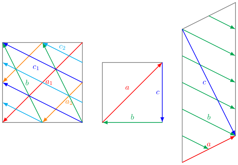
Refer to caption
Figure 2: Brane configuration for the three two-tori in Model 13 where the third two-torus is tilted. Fermion mass hierarchies result from the intersections on the first two-torus.
Table 3: The angles with respect to the orientifold plane made by the cycle wrapped by each stack of D-branes on each of the three two-tori in Model 13.

13θ1θ2θ3atan1(15)tan1(25)tan1(125)btan1(115)0π2ctan1(25)tan1(25)tan1(25)missing-subexpressionmissing-subexpressionmissing-subexpressionmissing-subexpression13superscript𝜃1superscript𝜃2superscript𝜃3missing-subexpressionmissing-subexpressionmissing-subexpressionmissing-subexpression𝑎superscript115superscript125superscript1125missing-subexpressionmissing-subexpressionmissing-subexpressionmissing-subexpression𝑏superscript11150𝜋2missing-subexpressionmissing-subexpressionmissing-subexpressionmissing-subexpression𝑐superscript125superscript125superscript125\begin{array}[]{|c|c|c|c|}\hline\cr\text{\hyperref@@ii[model13]{13}}&\theta^{1}&\theta^{2}&\theta^{3}\\ \hline\cr a&\tan^{-1}\left(\frac{1}{\sqrt{5}}\right)&-\tan^{-1}\left(\frac{2}{\sqrt{5}}\right)&-\tan^{-1}\left(\frac{1}{2\sqrt{5}}\right)\\ \hline\cr b&\tan^{-1}\left(\frac{11}{\sqrt{5}}\right)&0&\frac{\pi}{2}\\ \hline\cr c&\tan^{-1}\left(2\sqrt{5}\right)&\tan^{-1}\left(\frac{2}{\sqrt{5}}\right)&-\tan^{-1}\left(2\sqrt{5}\right)\\ \hline\cr\end{array}

The complex structure moduli U𝑈U from (18) are,

{U1,U2,U3}subscript𝑈1subscript𝑈2subscript𝑈3\displaystyle\{U_{1},U_{2},U_{3}\} ={i5,11i5,421(10+i5)},absent𝑖511𝑖542110𝑖5\displaystyle=\left\{\frac{i}{\sqrt{5}},\frac{11i}{\sqrt{5}},\frac{4}{21}\left(10+i\sqrt{5}\right)\right\}, (66)

and the corresponding u𝑢u-moduli and s𝑠s-modulus in supergravity basis from (19) are,

{u1,u2,u3}subscript𝑢1subscript𝑢2subscript𝑢3\displaystyle\{u_{1},u_{2},u_{3}\} ={5411eϕ4π,54eϕ411π,11eϕ44 53/4π},absent4511superscript𝑒subscriptitalic-ϕ4𝜋45superscript𝑒subscriptitalic-ϕ411𝜋11superscript𝑒subscriptitalic-ϕ4superscript4534𝜋\displaystyle=\left\{\frac{\sqrt[4]{5}\sqrt{11}e^{-\phi_{4}}}{\pi},\frac{\sqrt[4]{5}e^{-\phi_{4}}}{\sqrt{11}\pi},\frac{\sqrt{11}e^{-\phi_{4}}}{4\ 5^{3/4}\pi}\right\},
s𝑠\displaystyle s =54eϕ4411π.absent45superscript𝑒subscriptitalic-ϕ4411𝜋\displaystyle=\frac{\sqrt[4]{5}e^{-\phi_{4}}}{4\sqrt{11}\pi}. (67)

Using (24) and the values from the table A17, the gauge kinetic function becomes,

{fa,fb,fc}subscript𝑓𝑎subscript𝑓𝑏subscript𝑓𝑐\displaystyle\{f_{a},f_{b},f_{c}\} ={63eϕ48 53/411π,954eϕ41611π,2111eϕ416 53/4π},absent63superscript𝑒subscriptitalic-ϕ4superscript853411𝜋945superscript𝑒subscriptitalic-ϕ41611𝜋2111superscript𝑒subscriptitalic-ϕ4superscript16534𝜋\displaystyle=\left\{\frac{63e^{-\phi_{4}}}{8\ 5^{3/4}\sqrt{11}\pi},\frac{9\sqrt[4]{5}e^{-\phi_{4}}}{16\sqrt{11}\pi},\frac{21\sqrt{11}e^{-\phi_{4}}}{16\ 5^{3/4}\pi}\right\}, (68)

To calculate gaugino masses M1,2,3subscript𝑀123M_{1,2,3} respectively for U(1)YUsubscript1𝑌{\rm U}(1)_{Y}, SU(2)LSUsubscript2𝐿{\rm SU}(2)_{L} and SU(3)cSUsubscript3𝑐{\rm SU}(3)_{c} gauge groups, we first compute Ma,b,csubscript𝑀𝑎𝑏𝑐M_{a,b,c} using (3.2) as,

Masubscript𝑀𝑎\displaystyle M_{a} =m3/2(110Θ1+10Θ2+11Θ3+5Θ4)423,absentsubscript𝑚32110subscriptΘ110subscriptΘ211subscriptΘ35subscriptΘ4423\displaystyle=\frac{m_{3/2}(110\Theta_{1}+10\Theta_{2}+11\Theta_{3}+5\Theta_{4})}{42\sqrt{3}},
Mbsubscript𝑀𝑏\displaystyle M_{b} =m3/2(4Θ25Θ4)33,absentsubscript𝑚324subscriptΘ25subscriptΘ433\displaystyle=\frac{m_{3/2}(4\Theta_{2}-5\Theta_{4})}{3\sqrt{3}},
Mcsubscript𝑀𝑐\displaystyle M_{c} =m3/2(20Θ1+Θ3)73.absentsubscript𝑚3220subscriptΘ1subscriptΘ373\displaystyle=\frac{m_{3/2}(20\Theta_{1}+\Theta_{3})}{7\sqrt{3}}. (69)

Next, to compute the trilinear coupling and the sleptons mass-squared we require the angles, the differences of angles and their first and second order derivatives with respect to the moduli. In table 3 we show the angles (44) made by the cycle wrapped by each stack D6 branes with respect to the orientifold plane. The differences of the angles, θxyiθyiθxisuperscriptsubscript𝜃𝑥𝑦𝑖superscriptsubscript𝜃𝑦𝑖superscriptsubscript𝜃𝑥𝑖\theta_{xy}^{i}\equiv\theta_{y}^{i}-\theta_{x}^{i} are,

[{0.,0.,0.}{0.132923,0.228657,0.378919}{0.642663,0.0589537,0.298383}{0.132923,0.228657,0.378919}{0.,0.,0.}{0.50974,0.287611,0.080536}{0.642663,0.0589537,0.298383}{0.50974,0.287611,0.080536}{0.,0.,0.}]\displaystyle\hskip-10.00002pt\left[\begin{array}[]{ccc}\{0.,0.,0.\}&\{0.132923,-0.228657,0.378919\}&\{0.642663,0.0589537,0.298383\}\\ \{-0.132923,0.228657,-0.378919\}&\{0.,0.,0.\}&\{0.50974,0.287611,-0.080536\}\\ \{-0.642663,-0.0589537,-0.298383\}&\{-0.50974,-0.287611,0.080536\}&\{0.,0.,0.\}\\ \end{array}\right] (73)

To account for the negative angle differences it is convenient to define the sign function σxyisuperscriptsubscript𝜎𝑥𝑦𝑖\sigma_{xy}^{i}, which is 11-1 only for negative angle difference and +11+1 otherwise,

σxyi(1)1H(θxyi)superscriptsubscript𝜎𝑥𝑦𝑖superscript11𝐻superscriptsubscript𝜃𝑥𝑦𝑖\displaystyle\sigma_{xy}^{i}\equiv(-1)^{1-H(\theta_{xy}^{i})} =({1,1,1}{1,1,1}{1,1,1}{1,1,1}{1,1,1}{1,1,1}{1,1,1}{1,1,1}{1,1,1}),absent111111111111111111111111111\displaystyle=\left(\begin{array}[]{ccc}\{1,1,1\}&\{1,-1,1\}&\{1,1,1\}\\ \{-1,1,-1\}&\{1,1,1\}&\{1,1,-1\}\\ \{-1,-1,-1\}&\{-1,-1,1\}&\{1,1,1\}\\ \end{array}\right), (77)

where H(x)𝐻𝑥H(x) is the unit step function. And the function ηxysubscript𝜂𝑥𝑦\eta_{xy} can thus be defined by taking the product on the torus index i𝑖i as,

ηxyiσxyi=(111111111).subscript𝜂𝑥𝑦subscriptproduct𝑖superscriptsubscript𝜎𝑥𝑦𝑖111111111\eta_{xy}\equiv\prod_{i}\sigma_{xy}^{i}=\left(\begin{array}[]{ccc}1&-1&1\\ 1&1&-1\\ -1&1&1\\ \end{array}\right). (78)

Using the values of σxyisuperscriptsubscript𝜎𝑥𝑦𝑖\sigma_{xy}^{i} and ηxyisuperscriptsubscript𝜂𝑥𝑦𝑖\eta_{xy}^{i} in (60) we can compute the four cases of functions Ψ(θxy)Ψsubscript𝜃𝑥𝑦\Psi(\theta_{xy}) defined in (55) and (56). Similarly we calculate the derivative Ψ(θxyj)=dΨ(θxyj)dθxyjsuperscriptΨsubscriptsuperscript𝜃𝑗𝑥𝑦𝑑Ψsubscriptsuperscript𝜃𝑗𝑥𝑦𝑑subscriptsuperscript𝜃𝑗𝑥𝑦\Psi^{\prime}(\theta^{j}_{xy})=\frac{d\Psi(\theta^{j}_{xy})}{d\theta^{j}_{xy}} using equations (63), (3.3), (3.3) and the properties of digamma function ψ(0)(z)superscript𝜓0𝑧\psi^{(0)}(z) (3.3) while neglecting the contribution of the t𝑡t-moduli.

Utilizing above results while ignoring the CP-violating phases γisubscript𝛾𝑖\gamma_{i}, the the gaugino masses for the respective gauge groups U(1)YUsubscript1𝑌{\rm U}(1)_{Y}, SU(2)LSUsubscript2𝐿{\rm SU}(2)_{L} and SU(3)CSUsubscript3𝐶{\rm SU}(3)_{C}; the trilinear coupling (3.2); and squared-masses of squarks and sleptons (3.2) are obtained as follows,

MB~subscript𝑀~𝐵\displaystyle M_{\tilde{B}} MY=m3/2(176Θ1+4Θ2+11Θ3+2Θ4)633,absentsubscript𝑀𝑌subscript𝑚32176subscriptΘ14subscriptΘ211subscriptΘ32subscriptΘ4633\displaystyle\equiv M_{Y}=\frac{m_{3/2}(176\Theta_{1}+4\Theta_{2}+11\Theta_{3}+2\Theta_{4})}{63\sqrt{3}},
MW~subscript𝑀~𝑊\displaystyle M_{\tilde{W}} Mb=m3/2(4Θ25Θ4)33,absentsubscript𝑀𝑏subscript𝑚324subscriptΘ25subscriptΘ433\displaystyle\equiv M_{b}=\frac{m_{3/2}(4\Theta_{2}-5\Theta_{4})}{3\sqrt{3}},
Mg~subscript𝑀~𝑔\displaystyle M_{\tilde{g}} Ma=m3/2(110Θ1+10Θ2+11Θ3+5Θ4)423,absentsubscript𝑀𝑎subscript𝑚32110subscriptΘ110subscriptΘ211subscriptΘ35subscriptΘ4423\displaystyle\equiv M_{a}=\frac{m_{3/2}(110\Theta_{1}+10\Theta_{2}+11\Theta_{3}+5\Theta_{4})}{42\sqrt{3}},
A0subscript𝐴0\displaystyle A_{0} Aabc=m3/2(0.557548Θ11.13015Θ2+0.418029Θ30.462383Θ4),absentsubscript𝐴𝑎𝑏𝑐subscript𝑚320.557548subscriptΘ11.13015subscriptΘ20.418029subscriptΘ30.462383subscriptΘ4\displaystyle\equiv A_{abc}=m_{3/2}\Bigl{(}-0.557548\Theta_{1}-1.13015\Theta_{2}+0.418029\Theta_{3}-0.462383\Theta_{4}\Bigr{)},
mL2mab2subscriptsuperscript𝑚2𝐿subscriptsuperscript𝑚2𝑎𝑏\displaystyle m^{2}_{L}\equiv m^{2}_{ab} =m3/22(0.185098Θ120.0411881Θ1Θ21.44927Θ1Θ31.45644Θ1Θ4\displaystyle=m_{3/2}^{2}\Bigl{(}0.185098\Theta_{1}{}^{2}-0.0411881\Theta_{1}\Theta_{2}-1.44927\Theta_{1}\Theta_{3}-1.45644\Theta_{1}\Theta_{4}
+1.06435Θ220.969753Θ2Θ30.386382Θ2Θ40.290557Θ32\displaystyle\quad+1.06435\Theta_{2}{}^{2}-0.969753\Theta_{2}\Theta_{3}-0.386382\Theta_{2}\Theta_{4}-0.290557\Theta_{3}{}^{2}
+0.395625Θ3Θ41.0645Θ4+21),\displaystyle\quad+0.395625\Theta_{3}\Theta_{4}-1.0645\Theta_{4}{}^{2}+1\Bigr{)},
mR2mac2subscriptsuperscript𝑚2𝑅subscriptsuperscript𝑚2𝑎𝑐\displaystyle m^{2}_{R}\equiv m^{2}_{ac} =m3/22(2.63181Θ1+20.77203Θ1Θ2+1.29272Θ1Θ3+1.47197Θ1Θ4\displaystyle=m_{3/2}^{2}\Bigl{(}-2.63181\Theta_{1}{}^{2}+0.77203\Theta_{1}\Theta_{2}+1.29272\Theta_{1}\Theta_{3}+1.47197\Theta_{1}\Theta_{4}
2.51929Θ2+21.29272Θ2Θ3+0.844287Θ2Θ42.34591Θ32\displaystyle\quad-2.51929\Theta_{2}{}^{2}+1.29272\Theta_{2}\Theta_{3}+0.844287\Theta_{2}\Theta_{4}-2.34591\Theta_{3}{}^{2}
0.0442256Θ3Θ40.0470486Θ4+21).\displaystyle\quad-0.0442256\Theta_{3}\Theta_{4}-0.0470486\Theta_{4}{}^{2}+1\Bigr{)}. (79)

All soft terms are subject to the constraint (38).

4.2 Model 14

In Model 14 the three-point Yukawa couplings arise from the triplet intersections from the branes a𝑎a, b𝑏b and c𝑐c on the second two-torus with 6 pairs of Higgs from the 𝒩=2𝒩2\mathcal{N}=2 sector. Yukawa matrices for the Model 14 are of rank 3 and the three intersections required to form the disk diagrams for the Yukawa couplings all occur on the second torus as shown in figure 3.

Refer to caption
Figure 3: Brane configuration for the three two-tori in Model 14 where the third two-torus is tilted. Fermion mass hierarchies result from the intersections on the second two-torus.
Table 4: The angles with respect to the orientifold plane made by the cycle wrapped by each stack of D-branes on each of the three two-tori in Model 14.

14θ1θ2θ3a3π40π2b0π43π4cπ43π43π4missing-subexpressionmissing-subexpressionmissing-subexpressionmissing-subexpression14superscript𝜃1superscript𝜃2superscript𝜃3missing-subexpressionmissing-subexpressionmissing-subexpressionmissing-subexpression𝑎3𝜋40𝜋2missing-subexpressionmissing-subexpressionmissing-subexpressionmissing-subexpression𝑏0𝜋43𝜋4missing-subexpressionmissing-subexpressionmissing-subexpressionmissing-subexpression𝑐𝜋43𝜋43𝜋4\begin{array}[]{|c|c|c|c|}\hline\cr\text{\hyperref@@ii[model14]{14}}&\theta^{1}&\theta^{2}&\theta^{3}\\ \hline\cr a&\frac{3\pi}{4}&0&\frac{\pi}{2}\\ \hline\cr b&0&\frac{\pi}{4}&\frac{3\pi}{4}\\ \hline\cr c&\frac{\pi}{4}&\frac{3\pi}{4}&\frac{3\pi}{4}\\ \hline\cr\end{array}

The complex structure moduli U𝑈U from (18) are,

{U1,U2,U3}subscript𝑈1subscript𝑈2subscript𝑈3\displaystyle\{U_{1},U_{2},U_{3}\} ={i,i3,1+i},absent𝑖𝑖31𝑖\displaystyle=\left\{i,\frac{i}{3},1+i\right\}, (80)

and the corresponding u𝑢u-moduli and s𝑠s-modulus in supergravity basis from (19) are,

{u1,u2,u3}subscript𝑢1subscript𝑢2subscript𝑢3\displaystyle\{u_{1},u_{2},u_{3}\} ={eϕ46π,32eϕ4π,eϕ426π},absentsuperscript𝑒subscriptitalic-ϕ46𝜋32superscript𝑒subscriptitalic-ϕ4𝜋superscript𝑒subscriptitalic-ϕ426𝜋\displaystyle=\left\{\frac{e^{-\phi_{4}}}{\sqrt{6}\pi},\frac{\sqrt{\frac{3}{2}}e^{-\phi_{4}}}{\pi},\frac{e^{-\phi_{4}}}{2\sqrt{6}\pi}\right\},
s𝑠\displaystyle s =32eϕ42π.absent32superscript𝑒subscriptitalic-ϕ42𝜋\displaystyle=\frac{\sqrt{\frac{3}{2}}e^{-\phi_{4}}}{2\pi}. (81)

Using (24) and the values from the table A18, the gauge kinetic function becomes,

{fa,fb,fc}subscript𝑓𝑎subscript𝑓𝑏subscript𝑓𝑐\displaystyle\{f_{a},f_{b},f_{c}\} ={32eϕ44π,32eϕ44π,32eϕ44π},absent32superscript𝑒subscriptitalic-ϕ44𝜋32superscript𝑒subscriptitalic-ϕ44𝜋32superscript𝑒subscriptitalic-ϕ44𝜋\displaystyle=\left\{\frac{\sqrt{\frac{3}{2}}e^{-\phi_{4}}}{4\pi},\frac{\sqrt{\frac{3}{2}}e^{-\phi_{4}}}{4\pi},\frac{\sqrt{\frac{3}{2}}e^{-\phi_{4}}}{4\pi}\right\}, (82)

To calculate gaugino masses M1,2,3subscript𝑀123M_{1,2,3} respectively for U(1)YUsubscript1𝑌{\rm U}(1)_{Y}, SU(2)LSUsubscript2𝐿{\rm SU}(2)_{L} and SU(3)cSUsubscript3𝑐{\rm SU}(3)_{c} gauge groups, we first compute Ma,b,csubscript𝑀𝑎𝑏𝑐M_{a,b,c} using (3.2) as,

Masubscript𝑀𝑎\displaystyle M_{a} =123m3/2(Θ2Θ4),absent123subscript𝑚32subscriptΘ2subscriptΘ4\displaystyle=\frac{1}{2}\sqrt{3}m_{3/2}(\Theta_{2}-\Theta_{4}),
Mbsubscript𝑀𝑏\displaystyle M_{b} =123m3/2(Θ1Θ4),absent123subscript𝑚32subscriptΘ1subscriptΘ4\displaystyle=\frac{1}{2}\sqrt{3}m_{3/2}(\Theta_{1}-\Theta_{4}),
Mcsubscript𝑀𝑐\displaystyle M_{c} =123m3/2(Θ2+Θ3).absent123subscript𝑚32subscriptΘ2subscriptΘ3\displaystyle=\frac{1}{2}\sqrt{3}m_{3/2}(\Theta_{2}+\Theta_{3}). (83)

Next, to compute the trilinear coupling and the sleptons mass-squared we require the angles, the differences of angles and their first and second order derivatives with respect to the moduli. In table 4 we show the angles (44) made by the cycle wrapped by each stack D6 branes with respect to the orientifold plane. The differences of the angles, θxyiθyiθxisuperscriptsubscript𝜃𝑥𝑦𝑖superscriptsubscript𝜃𝑦𝑖superscriptsubscript𝜃𝑥𝑖\theta_{xy}^{i}\equiv\theta_{y}^{i}-\theta_{x}^{i} are,

[{0.,0.,0.}{0.0730092,0.643806,0.570796}{0.356194,0.356194,0.429204}{0.0730092,0.643806,0.570796}{0.,0.,0.}{0.429204,0.287611,0.141593}{0.356194,0.356194,0.429204}{0.429204,0.287611,0.141593}{0.,0.,0.}]\displaystyle\hskip-10.00002pt\left[\begin{array}[]{ccc}\{0.,0.,0.\}&\{-0.0730092,0.643806,-0.570796\}&\{0.356194,0.356194,-0.429204\}\\ \{0.0730092,-0.643806,0.570796\}&\{0.,0.,0.\}&\{0.429204,-0.287611,0.141593\}\\ \{-0.356194,-0.356194,0.429204\}&\{-0.429204,0.287611,-0.141593\}&\{0.,0.,0.\}\\ \end{array}\right] (87)

To account for the negative angle differences it is convenient to define the sign function σxyisuperscriptsubscript𝜎𝑥𝑦𝑖\sigma_{xy}^{i}, which is 11-1 only for negative angle difference and +11+1 otherwise,

σxyi(1)1H(θxyi)superscriptsubscript𝜎𝑥𝑦𝑖superscript11𝐻superscriptsubscript𝜃𝑥𝑦𝑖\displaystyle\sigma_{xy}^{i}\equiv(-1)^{1-H(\theta_{xy}^{i})} =({1,1,1}{1,1,1}{1,1,1}{1,1,1}{1,1,1}{1,1,1}{1,1,1}{1,1,1}{1,1,1}),absent111111111111111111111111111\displaystyle=\left(\begin{array}[]{ccc}\{1,1,1\}&\{-1,1,-1\}&\{1,1,-1\}\\ \{1,-1,1\}&\{1,1,1\}&\{1,-1,1\}\\ \{-1,-1,1\}&\{-1,1,-1\}&\{1,1,1\}\\ \end{array}\right), (91)

where H(x)𝐻𝑥H(x) is the unit step function. And the function ηxysubscript𝜂𝑥𝑦\eta_{xy} can thus be defined by taking the product on the torus index i𝑖i as,

ηxyiσxyi=(111111111).subscript𝜂𝑥𝑦subscriptproduct𝑖superscriptsubscript𝜎𝑥𝑦𝑖111111111\eta_{xy}\equiv\prod_{i}\sigma_{xy}^{i}=\left(\begin{array}[]{ccc}1&1&-1\\ -1&1&-1\\ 1&1&1\\ \end{array}\right). (92)

Using the values of σxyisuperscriptsubscript𝜎𝑥𝑦𝑖\sigma_{xy}^{i} and ηxyisuperscriptsubscript𝜂𝑥𝑦𝑖\eta_{xy}^{i} in (60) we can compute the four cases of functions Ψ(θxy)Ψsubscript𝜃𝑥𝑦\Psi(\theta_{xy}) defined in (55) and (56). Similarly we calculate the derivative Ψ(θxyj)=dΨ(θxyj)dθxyjsuperscriptΨsubscriptsuperscript𝜃𝑗𝑥𝑦𝑑Ψsubscriptsuperscript𝜃𝑗𝑥𝑦𝑑subscriptsuperscript𝜃𝑗𝑥𝑦\Psi^{\prime}(\theta^{j}_{xy})=\frac{d\Psi(\theta^{j}_{xy})}{d\theta^{j}_{xy}} using equations (63), (3.3), (3.3) and the properties of digamma function ψ(0)(z)superscript𝜓0𝑧\psi^{(0)}(z) (3.3) while neglecting the contribution of the t𝑡t-moduli.

Utilizing above results while ignoring the CP-violating phases γisubscript𝛾𝑖\gamma_{i}, the the gaugino masses for the respective gauge groups U(1)YUsubscript1𝑌{\rm U}(1)_{Y}, SU(2)LSUsubscript2𝐿{\rm SU}(2)_{L} and SU(3)CSUsubscript3𝐶{\rm SU}(3)_{C}; the trilinear coupling (3.2); and squared-masses of squarks and sleptons (3.2) are obtained as follows,

MB~subscript𝑀~𝐵\displaystyle M_{\tilde{B}} MY=1103m3/2(5Θ2+3Θ32Θ4),absentsubscript𝑀𝑌1103subscript𝑚325subscriptΘ23subscriptΘ32subscriptΘ4\displaystyle\equiv M_{Y}=\frac{1}{10}\sqrt{3}m_{3/2}(5\Theta_{2}+3\Theta_{3}-2\Theta_{4}),
MW~subscript𝑀~𝑊\displaystyle M_{\tilde{W}} Mb=123m3/2(Θ1Θ4),absentsubscript𝑀𝑏123subscript𝑚32subscriptΘ1subscriptΘ4\displaystyle\equiv M_{b}=\frac{1}{2}\sqrt{3}m_{3/2}(\Theta_{1}-\Theta_{4}),
Mg~subscript𝑀~𝑔\displaystyle M_{\tilde{g}} Ma=123m3/2(Θ2Θ4),absentsubscript𝑀𝑎123subscript𝑚32subscriptΘ2subscriptΘ4\displaystyle\equiv M_{a}=\frac{1}{2}\sqrt{3}m_{3/2}(\Theta_{2}-\Theta_{4}),
A0subscript𝐴0\displaystyle A_{0} Aabc=m3/2(0.444661Θ11.36219Θ2+0.260871Θ30.186075Θ4),absentsubscript𝐴𝑎𝑏𝑐subscript𝑚320.444661subscriptΘ11.36219subscriptΘ20.260871subscriptΘ30.186075subscriptΘ4\displaystyle\equiv A_{abc}=m_{3/2}\Bigl{(}-0.444661\Theta_{1}-1.36219\Theta_{2}+0.260871\Theta_{3}-0.186075\Theta_{4}\Bigr{)},
mL2mab2subscriptsuperscript𝑚2𝐿subscriptsuperscript𝑚2𝑎𝑏\displaystyle m^{2}_{L}\equiv m^{2}_{ab} =m3/22(0.0689562Θ1+21.52807Θ1Θ20.25782Θ1Θ30.582907Θ1Θ4\displaystyle=m_{3/2}^{2}\Bigl{(}-0.0689562\Theta_{1}{}^{2}+1.52807\Theta_{1}\Theta_{2}-0.25782\Theta_{1}\Theta_{3}-0.582907\Theta_{1}\Theta_{4}
0.127855Θ2+20.31395Θ2Θ30.623439Θ2Θ42.04994Θ32\displaystyle\quad-0.127855\Theta_{2}{}^{2}+0.31395\Theta_{2}\Theta_{3}-0.623439\Theta_{2}\Theta_{4}-2.04994\Theta_{3}{}^{2}
+1.23441Θ3Θ40.809377Θ4+21),\displaystyle\quad+1.23441\Theta_{3}\Theta_{4}-0.809377\Theta_{4}{}^{2}+1\Bigr{)},
mR2mac2subscriptsuperscript𝑚2𝑅subscriptsuperscript𝑚2𝑎𝑐\displaystyle m^{2}_{R}\equiv m^{2}_{ac} =m3/22(2.28519Θ121.00169Θ1Θ2+0.506454Θ1Θ3+1.26634Θ1Θ4\displaystyle=m_{3/2}^{2}\Bigl{(}-2.28519\Theta_{1}{}^{2}-1.00169\Theta_{1}\Theta_{2}+0.506454\Theta_{1}\Theta_{3}+1.26634\Theta_{1}\Theta_{4}
0.637087Θ2+21.13601Θ2Θ3+0.140834Θ2Θ40.0262168Θ32\displaystyle\quad-0.637087\Theta_{2}{}^{2}+1.13601\Theta_{2}\Theta_{3}+0.140834\Theta_{2}\Theta_{4}-0.0262168\Theta_{3}{}^{2}
1.1866Θ3Θ40.492648Θ4+21).\displaystyle\quad-1.1866\Theta_{3}\Theta_{4}-0.492648\Theta_{4}{}^{2}+1\Bigr{)}. (93)

All soft terms are subject to the constraint (38).

4.3 Model 15

In Model 15 the three-point Yukawa couplings arise from the triplet intersections from the branes a𝑎a, b𝑏b and c𝑐c on the first two-torus with 6 pairs of Higgs from the 𝒩=2𝒩2\mathcal{N}=2 sector. Yukawa matrices for the Model 15 are of rank 3 and the three intersections required to form the disk diagrams for the Yukawa couplings all occur on the first torus as shown in figure 4.
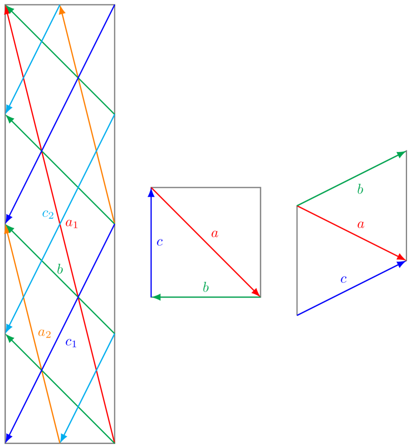
Refer to caption
Figure 4: Brane configuration for the three two-tori in Model 15 where the third two-torus is tilted. Fermion mass hierarchies result from the intersections on the first two-torus.
Table 5: The angles with respect to the orientifold plane made by the cycle wrapped by each stack of D-branes on each of the three two-tori in Model 15.

15θ1θ2θ3atan1(22)tan1(12)tan1(2)btan1(52)0π2ctan1(12)tan1(12)tan1(12)missing-subexpressionmissing-subexpressionmissing-subexpressionmissing-subexpression15superscript𝜃1superscript𝜃2superscript𝜃3missing-subexpressionmissing-subexpressionmissing-subexpressionmissing-subexpression𝑎superscript122superscript112superscript12missing-subexpressionmissing-subexpressionmissing-subexpressionmissing-subexpression𝑏superscript1520𝜋2missing-subexpressionmissing-subexpressionmissing-subexpressionmissing-subexpression𝑐superscript112superscript112superscript112\begin{array}[]{|c|c|c|c|}\hline\cr\text{\hyperref@@ii[model15]{15}}&\theta^{1}&\theta^{2}&\theta^{3}\\ \hline\cr a&-\tan^{-1}\left(2\sqrt{2}\right)&-\tan^{-1}\left(\frac{1}{\sqrt{2}}\right)&\tan^{-1}\left(\sqrt{2}\right)\\ \hline\cr b&-\tan^{-1}\left(\frac{5}{\sqrt{2}}\right)&0&\frac{\pi}{2}\\ \hline\cr c&-\tan^{-1}\left(\frac{1}{\sqrt{2}}\right)&\tan^{-1}\left(\frac{1}{\sqrt{2}}\right)&\tan^{-1}\left(\frac{1}{\sqrt{2}}\right)\\ \hline\cr\end{array}

The complex structure moduli U𝑈U from (18) are,

{U1,U2,U3}subscript𝑈1subscript𝑈2subscript𝑈3\displaystyle\{U_{1},U_{2},U_{3}\} ={2i2,5i2,23(1+i2)},absent2𝑖25𝑖2231𝑖2\displaystyle=\left\{2i\sqrt{2},\frac{5i}{\sqrt{2}},\frac{2}{3}\left(1+i\sqrt{2}\right)\right\}, (94)

and the corresponding u𝑢u-moduli and s𝑠s-modulus in supergravity basis from (19) are,

{u1,u2,u3}subscript𝑢1subscript𝑢2subscript𝑢3\displaystyle\{u_{1},u_{2},u_{3}\} ={5eϕ42 23/4π,24eϕ45π,5eϕ423/4π},absent5superscript𝑒subscriptitalic-ϕ4superscript2234𝜋42superscript𝑒subscriptitalic-ϕ45𝜋5superscript𝑒subscriptitalic-ϕ4superscript234𝜋\displaystyle=\left\{\frac{\sqrt{5}e^{-\phi_{4}}}{2\ 2^{3/4}\pi},\frac{\sqrt[4]{2}e^{-\phi_{4}}}{\sqrt{5}\pi},\frac{\sqrt{5}e^{-\phi_{4}}}{2^{3/4}\pi}\right\},
s𝑠\displaystyle s =eϕ42 23/45π.absentsuperscript𝑒subscriptitalic-ϕ4superscript22345𝜋\displaystyle=\frac{e^{-\phi_{4}}}{2\ 2^{3/4}\sqrt{5}\pi}. (95)

Using (24) and the values from the table A19, the gauge kinetic function becomes,

{fa,fb,fc}subscript𝑓𝑎subscript𝑓𝑏subscript𝑓𝑐\displaystyle\{f_{a},f_{b},f_{c}\} ={27eϕ416 23/45π,3eϕ44 23/45π,35eϕ48 23/4π},absent27superscript𝑒subscriptitalic-ϕ4superscript162345𝜋3superscript𝑒subscriptitalic-ϕ4superscript42345𝜋35superscript𝑒subscriptitalic-ϕ4superscript8234𝜋\displaystyle=\left\{\frac{27e^{-\phi_{4}}}{16\ 2^{3/4}\sqrt{5}\pi},\frac{3e^{-\phi_{4}}}{4\ 2^{3/4}\sqrt{5}\pi},\frac{3\sqrt{5}e^{-\phi_{4}}}{8\ 2^{3/4}\pi}\right\}, (96)

To calculate gaugino masses M1,2,3subscript𝑀123M_{1,2,3} respectively for U(1)YUsubscript1𝑌{\rm U}(1)_{Y}, SU(2)LSUsubscript2𝐿{\rm SU}(2)_{L} and SU(3)cSUsubscript3𝑐{\rm SU}(3)_{c} gauge groups, we first compute Ma,b,csubscript𝑀𝑎𝑏𝑐M_{a,b,c} using (3.2) as,

Masubscript𝑀𝑎\displaystyle M_{a} =m3/2(5Θ1+4Θ2+20Θ3+2Θ4)93,absentsubscript𝑚325subscriptΘ14subscriptΘ220subscriptΘ32subscriptΘ493\displaystyle=\frac{m_{3/2}(5\Theta_{1}+4\Theta_{2}+20\Theta_{3}+2\Theta_{4})}{9\sqrt{3}},
Mbsubscript𝑀𝑏\displaystyle M_{b} =m3/2(Θ22Θ4)3,absentsubscript𝑚32subscriptΘ22subscriptΘ43\displaystyle=\frac{m_{3/2}(\Theta_{2}-2\Theta_{4})}{\sqrt{3}},
Mcsubscript𝑀𝑐\displaystyle M_{c} =m3/2(Θ1+2Θ3)3.absentsubscript𝑚32subscriptΘ12subscriptΘ33\displaystyle=\frac{m_{3/2}(\Theta_{1}+2\Theta_{3})}{\sqrt{3}}. (97)

Next, to compute the trilinear coupling and the sleptons mass-squared we require the angles, the differences of angles and their first and second order derivatives with respect to the moduli. In table 5 we show the angles (44) made by the cycle wrapped by each stack D6 branes with respect to the orientifold plane. The differences of the angles, θxyiθyiθxisuperscriptsubscript𝜃𝑥𝑦𝑖superscriptsubscript𝜃𝑦𝑖superscriptsubscript𝜃𝑥𝑖\theta_{xy}^{i}\equiv\theta_{y}^{i}-\theta_{x}^{i} are,

[{0.,0.,0.}{0.38452,0.563254,0.230959}{0.0969093,0.13405,0.230959}{0.38452,0.563254,0.230959}{0.,0.,0.}{0.287611,0.429204,0.}{0.0969093,0.13405,0.230959}{0.287611,0.429204,0.}{0.,0.,0.}]\displaystyle\hskip-10.00002pt\left[\begin{array}[]{ccc}\{0.,0.,0.\}&\{-0.38452,-0.563254,0.230959\}&\{-0.0969093,-0.13405,0.230959\}\\ \{0.38452,0.563254,-0.230959\}&\{0.,0.,0.\}&\{0.287611,0.429204,0.\}\\ \{0.0969093,0.13405,-0.230959\}&\{-0.287611,-0.429204,0.\}&\{0.,0.,0.\}\\ \end{array}\right] (101)

To account for the negative angle differences it is convenient to define the sign function σxyisuperscriptsubscript𝜎𝑥𝑦𝑖\sigma_{xy}^{i}, which is 11-1 only for negative angle difference and +11+1 otherwise,

σxyi(1)1H(θxyi)superscriptsubscript𝜎𝑥𝑦𝑖superscript11𝐻superscriptsubscript𝜃𝑥𝑦𝑖\displaystyle\sigma_{xy}^{i}\equiv(-1)^{1-H(\theta_{xy}^{i})} =({1,1,1}{1,1,1}{1,1,1}{1,1,1}{1,1,1}{1,1,1}{1,1,1}{1,1,1}{1,1,1}),absent111111111111111111111111111\displaystyle=\left(\begin{array}[]{ccc}\{1,1,1\}&\{-1,-1,1\}&\{-1,-1,1\}\\ \{1,1,-1\}&\{1,1,1\}&\{1,1,1\}\\ \{1,1,-1\}&\{-1,-1,1\}&\{1,1,1\}\\ \end{array}\right), (105)

where H(x)𝐻𝑥H(x) is the unit step function. And the function ηxysubscript𝜂𝑥𝑦\eta_{xy} can thus be defined by taking the product on the torus index i𝑖i as,

ηxyiσxyi=(111111111).subscript𝜂𝑥𝑦subscriptproduct𝑖superscriptsubscript𝜎𝑥𝑦𝑖111111111\eta_{xy}\equiv\prod_{i}\sigma_{xy}^{i}=\left(\begin{array}[]{ccc}1&1&1\\ -1&1&1\\ -1&1&1\\ \end{array}\right). (106)

Using the values of σxyisuperscriptsubscript𝜎𝑥𝑦𝑖\sigma_{xy}^{i} and ηxyisuperscriptsubscript𝜂𝑥𝑦𝑖\eta_{xy}^{i} in (60) we can compute the four cases of functions Ψ(θxy)Ψsubscript𝜃𝑥𝑦\Psi(\theta_{xy}) defined in (55) and (56). Similarly we calculate the derivative Ψ(θxyj)=dΨ(θxyj)dθxyjsuperscriptΨsubscriptsuperscript𝜃𝑗𝑥𝑦𝑑Ψsubscriptsuperscript𝜃𝑗𝑥𝑦𝑑subscriptsuperscript𝜃𝑗𝑥𝑦\Psi^{\prime}(\theta^{j}_{xy})=\frac{d\Psi(\theta^{j}_{xy})}{d\theta^{j}_{xy}} using equations (63), (3.3), (3.3) and the properties of digamma function ψ(0)(z)superscript𝜓0𝑧\psi^{(0)}(z) (3.3) while neglecting the contribution of the t𝑡t-moduli.

Utilizing above results while ignoring the CP-violating phases γisubscript𝛾𝑖\gamma_{i}, the the gaugino masses for the respective gauge groups U(1)YUsubscript1𝑌{\rm U}(1)_{Y}, SU(2)LSUsubscript2𝐿{\rm SU}(2)_{L} and SU(3)CSUsubscript3𝐶{\rm SU}(3)_{C}; the trilinear coupling (3.2); and squared-masses of squarks and sleptons (3.2) are obtained as follows,

MB~subscript𝑀~𝐵\displaystyle M_{\tilde{B}} MY=m3/2(10Θ1+2Θ2+25Θ3+Θ4)123,absentsubscript𝑀𝑌subscript𝑚3210subscriptΘ12subscriptΘ225subscriptΘ3subscriptΘ4123\displaystyle\equiv M_{Y}=\frac{m_{3/2}(10\Theta_{1}+2\Theta_{2}+25\Theta_{3}+\Theta_{4})}{12\sqrt{3}},
MW~subscript𝑀~𝑊\displaystyle M_{\tilde{W}} Mb=m3/2(Θ22Θ4)3,absentsubscript𝑀𝑏subscript𝑚32subscriptΘ22subscriptΘ43\displaystyle\equiv M_{b}=\frac{m_{3/2}(\Theta_{2}-2\Theta_{4})}{\sqrt{3}},
Mg~subscript𝑀~𝑔\displaystyle M_{\tilde{g}} Ma=m3/2(5Θ1+4Θ2+20Θ3+2Θ4)93,absentsubscript𝑀𝑎subscript𝑚325subscriptΘ14subscriptΘ220subscriptΘ32subscriptΘ493\displaystyle\equiv M_{a}=\frac{m_{3/2}(5\Theta_{1}+4\Theta_{2}+20\Theta_{3}+2\Theta_{4})}{9\sqrt{3}},
A0subscript𝐴0\displaystyle A_{0} Aabc=m3/2(0.863715Θ1+0.764882Θ21.2303Θ30.402914Θ4),absentsubscript𝐴𝑎𝑏𝑐subscript𝑚320.863715subscriptΘ10.764882subscriptΘ21.2303subscriptΘ30.402914subscriptΘ4\displaystyle\equiv A_{abc}=m_{3/2}\Bigl{(}-0.863715\Theta_{1}+0.764882\Theta_{2}-1.2303\Theta_{3}-0.402914\Theta_{4}\Bigr{)},
mL2mab2subscriptsuperscript𝑚2𝐿subscriptsuperscript𝑚2𝑎𝑏\displaystyle m^{2}_{L}\equiv m^{2}_{ab} =m3/22(1.47868Θ120.544215Θ1Θ2+2.13294Θ1Θ3+0.574711Θ1Θ4\displaystyle=m_{3/2}^{2}\Bigl{(}-1.47868\Theta_{1}{}^{2}-0.544215\Theta_{1}\Theta_{2}+2.13294\Theta_{1}\Theta_{3}+0.574711\Theta_{1}\Theta_{4}
2.39151Θ2+21.01424Θ2Θ3+1.98343Θ2Θ4+0.200897Θ32\displaystyle\quad-2.39151\Theta_{2}{}^{2}+1.01424\Theta_{2}\Theta_{3}+1.98343\Theta_{2}\Theta_{4}+0.200897\Theta_{3}{}^{2}
1.60235Θ3Θ41.24227Θ4+21),\displaystyle\quad-1.60235\Theta_{3}\Theta_{4}-1.24227\Theta_{4}{}^{2}+1\Bigr{)},
mR2mac2subscriptsuperscript𝑚2𝑅subscriptsuperscript𝑚2𝑎𝑐\displaystyle m^{2}_{R}\equiv m^{2}_{ac} =m3/22(0.93815Θ120.630132Θ1Θ2+1.49955Θ1Θ3+1.27302Θ1Θ4\displaystyle=m_{3/2}^{2}\Bigl{(}-0.93815\Theta_{1}{}^{2}-0.630132\Theta_{1}\Theta_{2}+1.49955\Theta_{1}\Theta_{3}+1.27302\Theta_{1}\Theta_{4}
2.84613Θ2+21.49955Θ2Θ3+1.28512Θ2Θ40.482776Θ32\displaystyle\quad-2.84613\Theta_{2}{}^{2}+1.49955\Theta_{2}\Theta_{3}+1.28512\Theta_{2}\Theta_{4}-0.482776\Theta_{3}{}^{2}
1.68827Θ3Θ40.472685Θ4+21).\displaystyle\quad-1.68827\Theta_{3}\Theta_{4}-0.472685\Theta_{4}{}^{2}+1\Bigr{)}. (107)

All soft terms are subject to the constraint (38).

4.4 Model 15-dual

In Model 15-dual the three-point Yukawa couplings arise from the triplet intersections from the branes a𝑎a, b𝑏b and c𝑐c on the second two-torus with 6 pairs of Higgs from the 𝒩=2𝒩2\mathcal{N}=2 sector. Yukawa matrices for the Model 15-dual are of rank 3 and the three intersections required to form the disk diagrams for the Yukawa couplings all occur on the second torus as shown in figure 5.
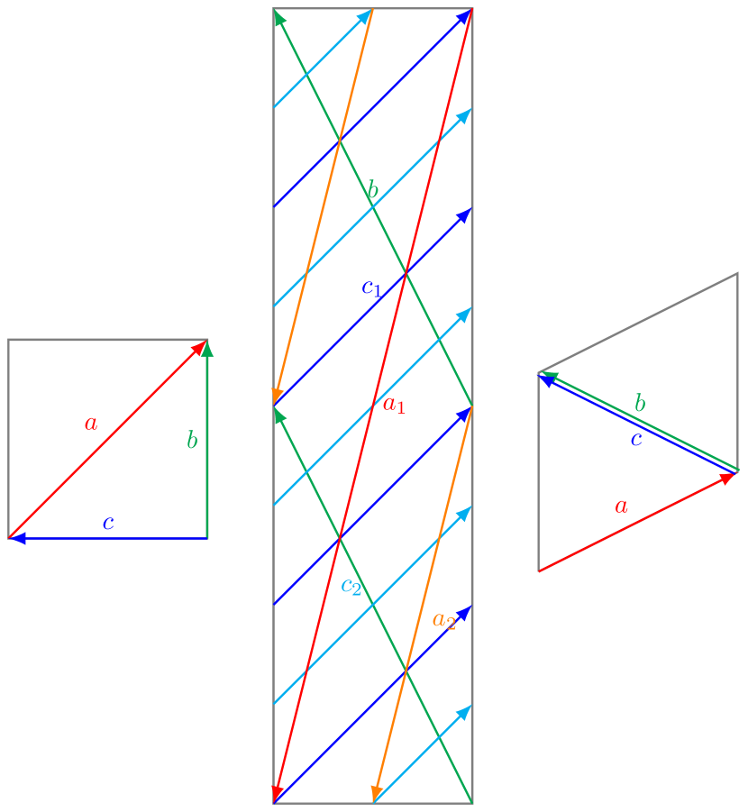
Refer to caption
Figure 5: Brane configuration for the three two-tori in Model 15-dual where the third two-torus is tilted. Fermion mass hierarchies result from the intersections on the second two-torus.
Table 6: The angles with respect to the orientifold plane made by the cycle wrapped by each stack of D-branes on each of the three two-tori in Model 15-dual.

15-dualθ1θ2θ3atan1(52)π20btan1(22)tan1(2)tan1(12)ctan1(12)tan1(12)tan1(12)missing-subexpressionmissing-subexpressionmissing-subexpressionmissing-subexpression15-dualsuperscript𝜃1superscript𝜃2superscript𝜃3missing-subexpressionmissing-subexpressionmissing-subexpressionmissing-subexpression𝑎superscript152𝜋20missing-subexpressionmissing-subexpressionmissing-subexpressionmissing-subexpression𝑏superscript122superscript12superscript112missing-subexpressionmissing-subexpressionmissing-subexpressionmissing-subexpression𝑐superscript112superscript112superscript112\begin{array}[]{|c|c|c|c|}\hline\cr\text{\hyperref@@ii[model15.5]{15-dual}}&\theta^{1}&\theta^{2}&\theta^{3}\\ \hline\cr a&\tan^{-1}\left(\frac{5}{\sqrt{2}}\right)&\frac{\pi}{2}&0\\ \hline\cr b&\tan^{-1}\left(2\sqrt{2}\right)&-\tan^{-1}\left(\sqrt{2}\right)&\tan^{-1}\left(\frac{1}{\sqrt{2}}\right)\\ \hline\cr c&\tan^{-1}\left(\frac{1}{\sqrt{2}}\right)&-\tan^{-1}\left(\frac{1}{\sqrt{2}}\right)&-\tan^{-1}\left(\frac{1}{\sqrt{2}}\right)\\ \hline\cr\end{array}

The complex structure moduli U𝑈U from (18) are,

{U1,U2,U3}subscript𝑈1subscript𝑈2subscript𝑈3\displaystyle\{U_{1},U_{2},U_{3}\} ={5i2,2i2,23(1+i2)},absent5𝑖22𝑖2231𝑖2\displaystyle=\left\{\frac{5i}{\sqrt{2}},2i\sqrt{2},\frac{2}{3}\left(1+i\sqrt{2}\right)\right\}, (108)

and the corresponding u𝑢u-moduli and s𝑠s-modulus in supergravity basis from (19) are,

{u1,u2,u3}subscript𝑢1subscript𝑢2subscript𝑢3\displaystyle\{u_{1},u_{2},u_{3}\} ={24eϕ45π,5eϕ42 23/4π,5eϕ423/4π},absent42superscript𝑒subscriptitalic-ϕ45𝜋5superscript𝑒subscriptitalic-ϕ4superscript2234𝜋5superscript𝑒subscriptitalic-ϕ4superscript234𝜋\displaystyle=\left\{\frac{\sqrt[4]{2}e^{-\phi_{4}}}{\sqrt{5}\pi},\frac{\sqrt{5}e^{-\phi_{4}}}{2\ 2^{3/4}\pi},\frac{\sqrt{5}e^{-\phi_{4}}}{2^{3/4}\pi}\right\},
s𝑠\displaystyle s =eϕ42 23/45π.absentsuperscript𝑒subscriptitalic-ϕ4superscript22345𝜋\displaystyle=\frac{e^{-\phi_{4}}}{2\ 2^{3/4}\sqrt{5}\pi}. (109)

Using (24) and the values from the table A20, the gauge kinetic function becomes,

{fa,fb,fc}subscript𝑓𝑎subscript𝑓𝑏subscript𝑓𝑐\displaystyle\{f_{a},f_{b},f_{c}\} ={27eϕ416 23/45π,35eϕ48 23/4π,3eϕ44 23/45π},absent27superscript𝑒subscriptitalic-ϕ4superscript162345𝜋35superscript𝑒subscriptitalic-ϕ4superscript8234𝜋3superscript𝑒subscriptitalic-ϕ4superscript42345𝜋\displaystyle=\left\{\frac{27e^{-\phi_{4}}}{16\ 2^{3/4}\sqrt{5}\pi},\frac{3\sqrt{5}e^{-\phi_{4}}}{8\ 2^{3/4}\pi},\frac{3e^{-\phi_{4}}}{4\ 2^{3/4}\sqrt{5}\pi}\right\}, (110)

To calculate gaugino masses M1,2,3subscript𝑀123M_{1,2,3} respectively for U(1)YUsubscript1𝑌{\rm U}(1)_{Y}, SU(2)LSUsubscript2𝐿{\rm SU}(2)_{L} and SU(3)cSUsubscript3𝑐{\rm SU}(3)_{c} gauge groups, we first compute Ma,b,csubscript𝑀𝑎𝑏𝑐M_{a,b,c} using (3.2) as,

Masubscript𝑀𝑎\displaystyle M_{a} =m3/2(4Θ1+5Θ2+20Θ3+2Θ4)93,absentsubscript𝑚324subscriptΘ15subscriptΘ220subscriptΘ32subscriptΘ493\displaystyle=\frac{m_{3/2}(4\Theta_{1}+5\Theta_{2}+20\Theta_{3}+2\Theta_{4})}{9\sqrt{3}},
Mbsubscript𝑀𝑏\displaystyle M_{b} =m3/2(Θ2+2Θ3)3,absentsubscript𝑚32subscriptΘ22subscriptΘ33\displaystyle=\frac{m_{3/2}(\Theta_{2}+2\Theta_{3})}{\sqrt{3}},
Mcsubscript𝑀𝑐\displaystyle M_{c} =m3/2(Θ12Θ4)3.absentsubscript𝑚32subscriptΘ12subscriptΘ43\displaystyle=\frac{m_{3/2}(\Theta_{1}-2\Theta_{4})}{\sqrt{3}}. (111)

Next, to compute the trilinear coupling and the sleptons mass-squared we require the angles, the differences of angles and their first and second order derivatives with respect to the moduli. In table 6 we show the angles (44) made by the cycle wrapped by each stack D6 branes with respect to the orientifold plane. The differences of the angles, θxyiθyiθxisuperscriptsubscript𝜃𝑥𝑦𝑖superscriptsubscript𝜃𝑦𝑖superscriptsubscript𝜃𝑥𝑖\theta_{xy}^{i}\equiv\theta_{y}^{i}-\theta_{x}^{i} are,

[{0.,0.,0.}{0.275643,0.0969093,0.0893668}{0.153561,0.526113,0.0893668}{0.275643,0.0969093,0.0893668}{0.,0.,0.}{0.429204,0.429204,0.}{0.153561,0.526113,0.0893668}{0.429204,0.429204,0.}{0.,0.,0.}]\displaystyle\hskip-10.00002pt\left[\begin{array}[]{ccc}\{0.,0.,0.\}&\{0.275643,0.0969093,-0.0893668\}&\{-0.153561,0.526113,-0.0893668\}\\ \{-0.275643,-0.0969093,0.0893668\}&\{0.,0.,0.\}&\{-0.429204,0.429204,0.\}\\ \{0.153561,-0.526113,0.0893668\}&\{0.429204,-0.429204,0.\}&\{0.,0.,0.\}\\ \end{array}\right] (115)

To account for the negative angle differences it is convenient to define the sign function σxyisuperscriptsubscript𝜎𝑥𝑦𝑖\sigma_{xy}^{i}, which is 11-1 only for negative angle difference and +11+1 otherwise,

σxyi(1)1H(θxyi)superscriptsubscript𝜎𝑥𝑦𝑖superscript11𝐻superscriptsubscript𝜃𝑥𝑦𝑖\displaystyle\sigma_{xy}^{i}\equiv(-1)^{1-H(\theta_{xy}^{i})} =({1,1,1}{1,1,1}{1,1,1}{1,1,1}{1,1,1}{1,1,1}{1,1,1}{1,1,1}{1,1,1}),absent111111111111111111111111111\displaystyle=\left(\begin{array}[]{ccc}\{1,1,1\}&\{1,1,-1\}&\{-1,1,-1\}\\ \{-1,-1,1\}&\{1,1,1\}&\{-1,1,1\}\\ \{1,-1,1\}&\{1,-1,1\}&\{1,1,1\}\\ \end{array}\right), (119)

where H(x)𝐻𝑥H(x) is the unit step function. And the function ηxysubscript𝜂𝑥𝑦\eta_{xy} can thus be defined by taking the product on the torus index i𝑖i as,

ηxyiσxyi=(111111111).subscript𝜂𝑥𝑦subscriptproduct𝑖superscriptsubscript𝜎𝑥𝑦𝑖111111111\eta_{xy}\equiv\prod_{i}\sigma_{xy}^{i}=\left(\begin{array}[]{ccc}1&-1&1\\ 1&1&-1\\ -1&-1&1\\ \end{array}\right). (120)

Using the values of σxyisuperscriptsubscript𝜎𝑥𝑦𝑖\sigma_{xy}^{i} and ηxyisuperscriptsubscript𝜂𝑥𝑦𝑖\eta_{xy}^{i} in (60) we can compute the four cases of functions Ψ(θxy)Ψsubscript𝜃𝑥𝑦\Psi(\theta_{xy}) defined in (55) and (56). Similarly we calculate the derivative Ψ(θxyj)=dΨ(θxyj)dθxyjsuperscriptΨsubscriptsuperscript𝜃𝑗𝑥𝑦𝑑Ψsubscriptsuperscript𝜃𝑗𝑥𝑦𝑑subscriptsuperscript𝜃𝑗𝑥𝑦\Psi^{\prime}(\theta^{j}_{xy})=\frac{d\Psi(\theta^{j}_{xy})}{d\theta^{j}_{xy}} using equations (63), (3.3), (3.3) and the properties of digamma function ψ(0)(z)superscript𝜓0𝑧\psi^{(0)}(z) (3.3) while neglecting the contribution of the t𝑡t-moduli.

Utilizing above results while ignoring the CP-violating phases γisubscript𝛾𝑖\gamma_{i}, the the gaugino masses for the respective gauge groups U(1)YUsubscript1𝑌{\rm U}(1)_{Y}, SU(2)LSUsubscript2𝐿{\rm SU}(2)_{L} and SU(3)CSUsubscript3𝐶{\rm SU}(3)_{C}; the trilinear coupling (3.2); and squared-masses of squarks and sleptons (3.2) are obtained as follows,

MB~subscript𝑀~𝐵\displaystyle M_{\tilde{B}} MY=m3/2(2Θ1+Θ2+4Θ32Θ4)33,absentsubscript𝑀𝑌subscript𝑚322subscriptΘ1subscriptΘ24subscriptΘ32subscriptΘ433\displaystyle\equiv M_{Y}=\frac{m_{3/2}(2\Theta_{1}+\Theta_{2}+4\Theta_{3}-2\Theta_{4})}{3\sqrt{3}},
MW~subscript𝑀~𝑊\displaystyle M_{\tilde{W}} Mb=m3/2(Θ2+2Θ3)3,absentsubscript𝑀𝑏subscript𝑚32subscriptΘ22subscriptΘ33\displaystyle\equiv M_{b}=\frac{m_{3/2}(\Theta_{2}+2\Theta_{3})}{\sqrt{3}},
Mg~subscript𝑀~𝑔\displaystyle M_{\tilde{g}} Ma=m3/2(4Θ1+5Θ2+20Θ3+2Θ4)93,absentsubscript𝑀𝑎subscript𝑚324subscriptΘ15subscriptΘ220subscriptΘ32subscriptΘ493\displaystyle\equiv M_{a}=\frac{m_{3/2}(4\Theta_{1}+5\Theta_{2}+20\Theta_{3}+2\Theta_{4})}{9\sqrt{3}},
A0subscript𝐴0\displaystyle A_{0} Aabc=m3/2(0.0762806Θ11.65577Θ2+0.222917Θ30.222917Θ4),absentsubscript𝐴𝑎𝑏𝑐subscript𝑚320.0762806subscriptΘ11.65577subscriptΘ20.222917subscriptΘ30.222917subscriptΘ4\displaystyle\equiv A_{abc}=m_{3/2}\Bigl{(}-0.0762806\Theta_{1}-1.65577\Theta_{2}+0.222917\Theta_{3}-0.222917\Theta_{4}\Bigr{)},
mL2mab2subscriptsuperscript𝑚2𝐿subscriptsuperscript𝑚2𝑎𝑏\displaystyle m^{2}_{L}\equiv m^{2}_{ab} =m3/22(2.50015Θ121.28868Θ1Θ2+0.56326Θ1Θ3+1.78275Θ1Θ4\displaystyle=m_{3/2}^{2}\Bigl{(}-2.50015\Theta_{1}{}^{2}-1.28868\Theta_{1}\Theta_{2}+0.56326\Theta_{1}\Theta_{3}+1.78275\Theta_{1}\Theta_{4}
0.272045Θ2+21.18291Θ2Θ3+0.336724Θ2Θ4+0.10754Θ32\displaystyle\quad-0.272045\Theta_{2}{}^{2}+1.18291\Theta_{2}\Theta_{3}+0.336724\Theta_{2}\Theta_{4}+0.10754\Theta_{3}{}^{2}
2.1859Θ3Θ40.202498Θ4+21),\displaystyle\quad-2.1859\Theta_{3}\Theta_{4}-0.202498\Theta_{4}{}^{2}+1\Bigr{)},
mR2mac2subscriptsuperscript𝑚2𝑅subscriptsuperscript𝑚2𝑎𝑐\displaystyle m^{2}_{R}\equiv m^{2}_{ac} =m3/22(0.229829Θ1+21.01289Θ1Θ20.749437Θ1Θ31.33965Θ1Θ4\displaystyle=m_{3/2}^{2}\Bigl{(}-0.229829\Theta_{1}{}^{2}+1.01289\Theta_{1}\Theta_{2}-0.749437\Theta_{1}\Theta_{3}-1.33965\Theta_{1}\Theta_{4}
+0.277823Θ220.150917Θ2Θ30.779826Θ2Θ41.85574Θ32\displaystyle\quad+0.277823\Theta_{2}{}^{2}-0.150917\Theta_{2}\Theta_{3}-0.779826\Theta_{2}\Theta_{4}-1.85574\Theta_{3}{}^{2}
+1.9101Θ3Θ40.7735Θ4+21).\displaystyle\quad+1.9101\Theta_{3}\Theta_{4}-0.7735\Theta_{4}{}^{2}+1\Bigr{)}. (121)

All soft terms are subject to the constraint (38).

4.5 Model 16

In Model 16 the three-point Yukawa couplings arise from the triplet intersections from the branes a𝑎a, b𝑏b and c𝑐c on the first two-torus with 6 pairs of Higgs from the 𝒩=2𝒩2\mathcal{N}=2 sector. Yukawa matrices for the Model 16 are of rank 3 and the three intersections required to form the disk diagrams for the Yukawa couplings all occur on the first torus as shown in figure 6.
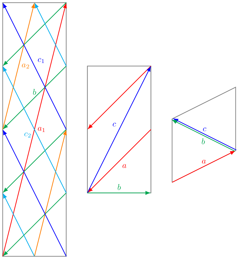
Refer to caption
Figure 6: Brane configuration for the three two-tori in Model 16 where the third two-torus is tilted. Fermion mass hierarchies result from the intersections on the first two-torus.
Table 7: The angles with respect to the orientifold plane made by the cycle wrapped by each stack of D-branes on each of the three two-tori in Model 16.

16θ1θ2θ3atan1(132)tan1(1324)tan1(1322)btan1(26)0tan1(226)ctan1(1324)tan1(1324)tan1(1324)missing-subexpressionmissing-subexpressionmissing-subexpressionmissing-subexpression16superscript𝜃1superscript𝜃2superscript𝜃3missing-subexpressionmissing-subexpressionmissing-subexpressionmissing-subexpression𝑎superscript1132superscript11324superscript11322missing-subexpressionmissing-subexpressionmissing-subexpressionmissing-subexpression𝑏superscript1260superscript1226missing-subexpressionmissing-subexpressionmissing-subexpressionmissing-subexpression𝑐superscript11324superscript11324superscript11324\begin{array}[]{|c|c|c|c|}\hline\cr\text{\hyperref@@ii[model16]{16}}&\theta^{1}&\theta^{2}&\theta^{3}\\ \hline\cr a&\tan^{-1}\left(\sqrt{\frac{13}{2}}\right)&\tan^{-1}\left(\frac{\sqrt{\frac{13}{2}}}{4}\right)&-\tan^{-1}\left(\frac{\sqrt{\frac{13}{2}}}{2}\right)\\ \hline\cr b&\tan^{-1}\left(\sqrt{26}\right)&0&\tan^{-1}\left(2\sqrt{26}\right)\\ \hline\cr c&\tan^{-1}\left(\frac{\sqrt{\frac{13}{2}}}{4}\right)&-\tan^{-1}\left(\frac{\sqrt{\frac{13}{2}}}{4}\right)&-\tan^{-1}\left(\frac{\sqrt{\frac{13}{2}}}{4}\right)\\ \hline\cr\end{array}

The complex structure moduli U𝑈U from (18) are,

{U1,U2,U3}subscript𝑈1subscript𝑈2subscript𝑈3\displaystyle\{U_{1},U_{2},U_{3}\} ={i132,2i26,245(13+4i26)},absent𝑖1322𝑖26245134𝑖26\displaystyle=\left\{i\sqrt{\frac{13}{2}},2i\sqrt{26},\frac{2}{45}\left(13+4i\sqrt{26}\right)\right\}, (122)

and the corresponding u𝑢u-moduli and s𝑠s-modulus in supergravity basis from (19) are,

{u1,u2,u3}subscript𝑢1subscript𝑢2subscript𝑢3\displaystyle\{u_{1},u_{2},u_{3}\} ={134eϕ423/4π,134eϕ44 23/4π,264eϕ4π},absent413superscript𝑒subscriptitalic-ϕ4superscript234𝜋413superscript𝑒subscriptitalic-ϕ4superscript4234𝜋426superscript𝑒subscriptitalic-ϕ4𝜋\displaystyle=\left\{\frac{\sqrt[4]{13}e^{-\phi_{4}}}{2^{3/4}\pi},\frac{\sqrt[4]{13}e^{-\phi_{4}}}{4\ 2^{3/4}\pi},\frac{\sqrt[4]{26}e^{-\phi_{4}}}{\pi}\right\},
s𝑠\displaystyle s =eϕ4263/4π.absentsuperscript𝑒subscriptitalic-ϕ4superscript2634𝜋\displaystyle=\frac{e^{-\phi_{4}}}{26^{3/4}\pi}. (123)

Using (24) and the values from the table A21, the gauge kinetic function becomes,

{fa,fb,fc}subscript𝑓𝑎subscript𝑓𝑏subscript𝑓𝑐\displaystyle\{f_{a},f_{b},f_{c}\} ={135eϕ416 263/4π,45eϕ432 263/4π,315eϕ432 263/4π},absent135superscript𝑒subscriptitalic-ϕ4superscript162634𝜋45superscript𝑒subscriptitalic-ϕ4superscript322634𝜋315superscript𝑒subscriptitalic-ϕ4superscript322634𝜋\displaystyle=\left\{\frac{135e^{-\phi_{4}}}{16\ 26^{3/4}\pi},\frac{45e^{-\phi_{4}}}{32\ 26^{3/4}\pi},\frac{315e^{-\phi_{4}}}{32\ 26^{3/4}\pi}\right\}, (124)

To calculate gaugino masses M1,2,3subscript𝑀123M_{1,2,3} respectively for U(1)YUsubscript1𝑌{\rm U}(1)_{Y}, SU(2)LSUsubscript2𝐿{\rm SU}(2)_{L} and SU(3)cSUsubscript3𝑐{\rm SU}(3)_{c} gauge groups, we first compute Ma,b,csubscript𝑀𝑎𝑏𝑐M_{a,b,c} using (3.2) as,

Masubscript𝑀𝑎\displaystyle M_{a} =m3/2(26Θ1+13Θ2+8(13Θ3+Θ4))453,absentsubscript𝑚3226subscriptΘ113subscriptΘ2813subscriptΘ3subscriptΘ4453\displaystyle=\frac{m_{3/2}(26\Theta_{1}+13\Theta_{2}+8(13\Theta_{3}+\Theta_{4}))}{45\sqrt{3}},
Mbsubscript𝑀𝑏\displaystyle M_{b} =m3/2(13Θ232Θ4)153,absentsubscript𝑚3213subscriptΘ232subscriptΘ4153\displaystyle=\frac{m_{3/2}(13\Theta_{2}-32\Theta_{4})}{15\sqrt{3}},
Mcsubscript𝑀𝑐\displaystyle M_{c} =m3/2(104Θ113Θ2+208Θ316Θ4)1053.absentsubscript𝑚32104subscriptΘ113subscriptΘ2208subscriptΘ316subscriptΘ41053\displaystyle=\frac{m_{3/2}(104\Theta_{1}-13\Theta_{2}+208\Theta_{3}-16\Theta_{4})}{105\sqrt{3}}. (125)

Next, to compute the trilinear coupling and the sleptons mass-squared we require the angles, the differences of angles and their first and second order derivatives with respect to the moduli. In table 7 we show the angles (44) made by the cycle wrapped by each stack D6 branes with respect to the orientifold plane. The differences of the angles, θxyiθyiθxisuperscriptsubscript𝜃𝑥𝑦𝑖superscriptsubscript𝜃𝑦𝑖superscriptsubscript𝜃𝑥𝑖\theta_{xy}^{i}\equiv\theta_{y}^{i}-\theta_{x}^{i} are,

[{0.,0.,0.}{0.228854,0.235545,0.0066917}{0.0389882,0.237505,0.0066917}{0.228854,0.235545,0.0066917}{0.,0.,0.}{0.189865,0.473051,0.}{0.0389882,0.237505,0.0066917}{0.189865,0.473051,0.}{0.,0.,0.}]\displaystyle\hskip-10.00002pt\left[\begin{array}[]{ccc}\{0.,0.,0.\}&\{0.228854,-0.235545,0.0066917\}&\{0.0389882,0.237505,0.0066917\}\\ \{-0.228854,0.235545,-0.0066917\}&\{0.,0.,0.\}&\{-0.189865,0.473051,0.\}\\ \{-0.0389882,-0.237505,-0.0066917\}&\{0.189865,-0.473051,0.\}&\{0.,0.,0.\}\\ \end{array}\right] (129)

To account for the negative angle differences it is convenient to define the sign function σxyisuperscriptsubscript𝜎𝑥𝑦𝑖\sigma_{xy}^{i}, which is 11-1 only for negative angle difference and +11+1 otherwise,

σxyi(1)1H(θxyi)superscriptsubscript𝜎𝑥𝑦𝑖superscript11𝐻superscriptsubscript𝜃𝑥𝑦𝑖\displaystyle\sigma_{xy}^{i}\equiv(-1)^{1-H(\theta_{xy}^{i})} =({1,1,1}{1,1,1}{1,1,1}{1,1,1}{1,1,1}{1,1,1}{1,1,1}{1,1,1}{1,1,1}),absent111111111111111111111111111\displaystyle=\left(\begin{array}[]{ccc}\{1,1,1\}&\{1,-1,1\}&\{1,1,1\}\\ \{-1,1,-1\}&\{1,1,1\}&\{-1,1,1\}\\ \{-1,-1,-1\}&\{1,-1,1\}&\{1,1,1\}\\ \end{array}\right), (133)

where H(x)𝐻𝑥H(x) is the unit step function. And the function ηxysubscript𝜂𝑥𝑦\eta_{xy} can thus be defined by taking the product on the torus index i𝑖i as,

ηxyiσxyi=(111111111).subscript𝜂𝑥𝑦subscriptproduct𝑖superscriptsubscript𝜎𝑥𝑦𝑖111111111\eta_{xy}\equiv\prod_{i}\sigma_{xy}^{i}=\left(\begin{array}[]{ccc}1&-1&1\\ 1&1&-1\\ -1&-1&1\\ \end{array}\right). (134)

Using the values of σxyisuperscriptsubscript𝜎𝑥𝑦𝑖\sigma_{xy}^{i} and ηxyisuperscriptsubscript𝜂𝑥𝑦𝑖\eta_{xy}^{i} in (60) we can compute the four cases of functions Ψ(θxy)Ψsubscript𝜃𝑥𝑦\Psi(\theta_{xy}) defined in (55) and (56). Similarly we calculate the derivative Ψ(θxyj)=dΨ(θxyj)dθxyjsuperscriptΨsubscriptsuperscript𝜃𝑗𝑥𝑦𝑑Ψsubscriptsuperscript𝜃𝑗𝑥𝑦𝑑subscriptsuperscript𝜃𝑗𝑥𝑦\Psi^{\prime}(\theta^{j}_{xy})=\frac{d\Psi(\theta^{j}_{xy})}{d\theta^{j}_{xy}} using equations (63), (3.3), (3.3) and the properties of digamma function ψ(0)(z)superscript𝜓0𝑧\psi^{(0)}(z) (3.3) while neglecting the contribution of the t𝑡t-moduli.

Utilizing above results while ignoring the CP-violating phases γisubscript𝛾𝑖\gamma_{i}, the the gaugino masses for the respective gauge groups U(1)YUsubscript1𝑌{\rm U}(1)_{Y}, SU(2)LSUsubscript2𝐿{\rm SU}(2)_{L} and SU(3)CSUsubscript3𝐶{\rm SU}(3)_{C}; the trilinear coupling (3.2); and squared-masses of squarks and sleptons (3.2) are obtained as follows,

MB~subscript𝑀~𝐵\displaystyle M_{\tilde{B}} MY=m3/2(416Θ1+13Θ2+1040Θ316Θ4)4953,absentsubscript𝑀𝑌subscript𝑚32416subscriptΘ113subscriptΘ21040subscriptΘ316subscriptΘ44953\displaystyle\equiv M_{Y}=\frac{m_{3/2}(416\Theta_{1}+13\Theta_{2}+1040\Theta_{3}-16\Theta_{4})}{495\sqrt{3}},
MW~subscript𝑀~𝑊\displaystyle M_{\tilde{W}} Mb=m3/2(13Θ232Θ4)153,absentsubscript𝑀𝑏subscript𝑚3213subscriptΘ232subscriptΘ4153\displaystyle\equiv M_{b}=\frac{m_{3/2}(13\Theta_{2}-32\Theta_{4})}{15\sqrt{3}},
Mg~subscript𝑀~𝑔\displaystyle M_{\tilde{g}} Ma=m3/2(26Θ1+13Θ2+8(13Θ3+Θ4))453,absentsubscript𝑀𝑎subscript𝑚3226subscriptΘ113subscriptΘ2813subscriptΘ3subscriptΘ4453\displaystyle\equiv M_{a}=\frac{m_{3/2}(26\Theta_{1}+13\Theta_{2}+8(13\Theta_{3}+\Theta_{4}))}{45\sqrt{3}},
A0subscript𝐴0\displaystyle A_{0} Aabc=m3/2(0.674714Θ11.05734Θ20.296892Θ3+0.296892Θ4),absentsubscript𝐴𝑎𝑏𝑐subscript𝑚320.674714subscriptΘ11.05734subscriptΘ20.296892subscriptΘ30.296892subscriptΘ4\displaystyle\equiv A_{abc}=m_{3/2}\Bigl{(}-0.674714\Theta_{1}-1.05734\Theta_{2}-0.296892\Theta_{3}+0.296892\Theta_{4}\Bigr{)},
mL2mab2subscriptsuperscript𝑚2𝐿subscriptsuperscript𝑚2𝑎𝑏\displaystyle m^{2}_{L}\equiv m^{2}_{ab} =m3/22(0.357659Θ1+20.87063Θ1Θ21.16965Θ1Θ30.902287Θ1Θ4\displaystyle=m_{3/2}^{2}\Bigl{(}0.357659\Theta_{1}{}^{2}+0.87063\Theta_{1}\Theta_{2}-1.16965\Theta_{1}\Theta_{3}-0.902287\Theta_{1}\Theta_{4}
0.152099Θ220.139037Θ2Θ31.26422Θ2Θ40.463359Θ32\displaystyle\quad-0.152099\Theta_{2}{}^{2}-0.139037\Theta_{2}\Theta_{3}-1.26422\Theta_{2}\Theta_{4}-0.463359\Theta_{3}{}^{2}
+1.81488Θ3Θ42.03894Θ4+21),\displaystyle\quad+1.81488\Theta_{3}\Theta_{4}-2.03894\Theta_{4}{}^{2}+1\Bigr{)},
mR2mac2subscriptsuperscript𝑚2𝑅subscriptsuperscript𝑚2𝑎𝑐\displaystyle m^{2}_{R}\equiv m^{2}_{ac} =m3/22(2.30496Θ120.638749Θ1Θ2+0.0264302Θ1Θ3+1.87359Θ1Θ4\displaystyle=m_{3/2}^{2}\Bigl{(}-2.30496\Theta_{1}{}^{2}-0.638749\Theta_{1}\Theta_{2}+0.0264302\Theta_{1}\Theta_{3}+1.87359\Theta_{1}\Theta_{4}
1.13248Θ2+20.518024Θ2Θ3+0.292916Θ2Θ40.63835Θ32\displaystyle\quad-1.13248\Theta_{2}{}^{2}+0.518024\Theta_{2}\Theta_{3}+0.292916\Theta_{2}\Theta_{4}-0.63835\Theta_{3}{}^{2}
1.58299Θ3Θ40.0912327Θ4+21).\displaystyle\quad-1.58299\Theta_{3}\Theta_{4}-0.0912327\Theta_{4}{}^{2}+1\Bigr{)}. (135)

All soft terms are subject to the constraint (38).

4.6 Model 16-dual

In Model 16-dual the three-point Yukawa couplings arise from the triplet intersections from the branes a𝑎a, b𝑏b and c𝑐c on the first two-torus with 6 pairs of Higgs from the 𝒩=2𝒩2\mathcal{N}=2 sector. Yukawa matrices for the Model 16-dual are of rank 3 and the three intersections required to form the disk diagrams for the Yukawa couplings all occur on the first torus as shown in figure 7.
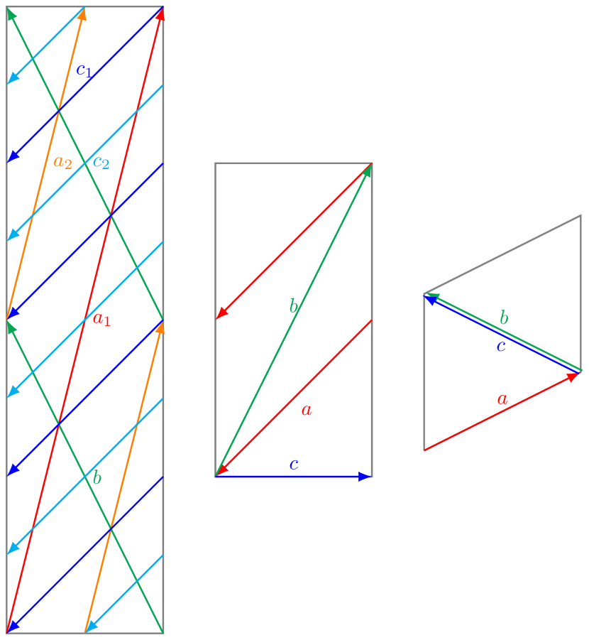
Refer to caption
Figure 7: Brane configuration for the three two-tori in Model 16-dual where the third two-torus is tilted. Fermion mass hierarchies result from the intersections on the first two-torus.
Table 8: The angles with respect to the orientifold plane made by the cycle wrapped by each stack of D-branes on each of the three two-tori in Model 16-dual.

16-dualθ1θ2θ3atan1(132)tan1(1322)tan1(1324)btan1(26)tan1(226)0ctan1(1324)tan1(1324)tan1(1324)missing-subexpressionmissing-subexpressionmissing-subexpressionmissing-subexpression16-dualsuperscript𝜃1superscript𝜃2superscript𝜃3missing-subexpressionmissing-subexpressionmissing-subexpressionmissing-subexpression𝑎superscript1132superscript11322superscript11324missing-subexpressionmissing-subexpressionmissing-subexpressionmissing-subexpression𝑏superscript126superscript12260missing-subexpressionmissing-subexpressionmissing-subexpressionmissing-subexpression𝑐superscript11324superscript11324superscript11324\begin{array}[]{|c|c|c|c|}\hline\cr\text{\hyperref@@ii[model16.5]{16-dual}}&\theta^{1}&\theta^{2}&\theta^{3}\\ \hline\cr a&\tan^{-1}\left(\sqrt{\frac{13}{2}}\right)&-\tan^{-1}\left(\frac{\sqrt{\frac{13}{2}}}{2}\right)&\tan^{-1}\left(\frac{\sqrt{\frac{13}{2}}}{4}\right)\\ \hline\cr b&\tan^{-1}\left(\sqrt{26}\right)&\tan^{-1}\left(2\sqrt{26}\right)&0\\ \hline\cr c&\tan^{-1}\left(\frac{\sqrt{\frac{13}{2}}}{4}\right)&-\tan^{-1}\left(\frac{\sqrt{\frac{13}{2}}}{4}\right)&-\tan^{-1}\left(\frac{\sqrt{\frac{13}{2}}}{4}\right)\\ \hline\cr\end{array}

The complex structure moduli U𝑈U from (18) are,

{U1,U2,U3}subscript𝑈1subscript𝑈2subscript𝑈3\displaystyle\{U_{1},U_{2},U_{3}\} ={i132,2i26,245(13+4i26)},absent𝑖1322𝑖26245134𝑖26\displaystyle=\left\{i\sqrt{\frac{13}{2}},2i\sqrt{26},\frac{2}{45}\left(13+4i\sqrt{26}\right)\right\}, (136)

and the corresponding u𝑢u-moduli and s𝑠s-modulus in supergravity basis from (19) are,

{u1,u2,u3}subscript𝑢1subscript𝑢2subscript𝑢3\displaystyle\{u_{1},u_{2},u_{3}\} ={134eϕ423/4π,134eϕ44 23/4π,264eϕ4π},absent413superscript𝑒subscriptitalic-ϕ4superscript234𝜋413superscript𝑒subscriptitalic-ϕ4superscript4234𝜋426superscript𝑒subscriptitalic-ϕ4𝜋\displaystyle=\left\{\frac{\sqrt[4]{13}e^{-\phi_{4}}}{2^{3/4}\pi},\frac{\sqrt[4]{13}e^{-\phi_{4}}}{4\ 2^{3/4}\pi},\frac{\sqrt[4]{26}e^{-\phi_{4}}}{\pi}\right\},
s𝑠\displaystyle s =eϕ4263/4π.absentsuperscript𝑒subscriptitalic-ϕ4superscript2634𝜋\displaystyle=\frac{e^{-\phi_{4}}}{26^{3/4}\pi}. (137)

Using (24) and the values from the table A22, the gauge kinetic function becomes,

{fa,fb,fc}subscript𝑓𝑎subscript𝑓𝑏subscript𝑓𝑐\displaystyle\{f_{a},f_{b},f_{c}\} ={135eϕ416 263/4π,315eϕ432 263/4π,45eϕ432 263/4π},absent135superscript𝑒subscriptitalic-ϕ4superscript162634𝜋315superscript𝑒subscriptitalic-ϕ4superscript322634𝜋45superscript𝑒subscriptitalic-ϕ4superscript322634𝜋\displaystyle=\left\{\frac{135e^{-\phi_{4}}}{16\ 26^{3/4}\pi},\frac{315e^{-\phi_{4}}}{32\ 26^{3/4}\pi},\frac{45e^{-\phi_{4}}}{32\ 26^{3/4}\pi}\right\}, (138)

To calculate gaugino masses M1,2,3subscript𝑀123M_{1,2,3} respectively for U(1)YUsubscript1𝑌{\rm U}(1)_{Y}, SU(2)LSUsubscript2𝐿{\rm SU}(2)_{L} and SU(3)cSUsubscript3𝑐{\rm SU}(3)_{c} gauge groups, we first compute Ma,b,csubscript𝑀𝑎𝑏𝑐M_{a,b,c} using (3.2) as,

Masubscript𝑀𝑎\displaystyle M_{a} =m3/2(26Θ1+13Θ2+8(13Θ3+Θ4))453,absentsubscript𝑚3226subscriptΘ113subscriptΘ2813subscriptΘ3subscriptΘ4453\displaystyle=\frac{m_{3/2}(26\Theta_{1}+13\Theta_{2}+8(13\Theta_{3}+\Theta_{4}))}{45\sqrt{3}},
Mbsubscript𝑀𝑏\displaystyle M_{b} =m3/2(104Θ113Θ2+208Θ316Θ4)1053,absentsubscript𝑚32104subscriptΘ113subscriptΘ2208subscriptΘ316subscriptΘ41053\displaystyle=\frac{m_{3/2}(104\Theta_{1}-13\Theta_{2}+208\Theta_{3}-16\Theta_{4})}{105\sqrt{3}},
Mcsubscript𝑀𝑐\displaystyle M_{c} =m3/2(13Θ232Θ4)153.absentsubscript𝑚3213subscriptΘ232subscriptΘ4153\displaystyle=\frac{m_{3/2}(13\Theta_{2}-32\Theta_{4})}{15\sqrt{3}}. (139)

Next, to compute the trilinear coupling and the sleptons mass-squared we require the angles, the differences of angles and their first and second order derivatives with respect to the moduli. In table 8 we show the angles (44) made by the cycle wrapped by each stack D6 branes with respect to the orientifold plane. The differences of the angles, θxyiθyiθxisuperscriptsubscript𝜃𝑥𝑦𝑖superscriptsubscript𝜃𝑦𝑖superscriptsubscript𝜃𝑥𝑖\theta_{xy}^{i}\equiv\theta_{y}^{i}-\theta_{x}^{i} are,

[{0.,0.,0.}{0.0389882,0.237505,0.0066917}{0.228854,0.235545,0.0066917}{0.0389882,0.237505,0.0066917}{0.,0.,0.}{0.189865,0.473051,0.}{0.228854,0.235545,0.0066917}{0.189865,0.473051,0.}{0.,0.,0.}]\displaystyle\hskip-10.00002pt\left[\begin{array}[]{ccc}\{0.,0.,0.\}&\{0.0389882,0.237505,0.0066917\}&\{0.228854,-0.235545,0.0066917\}\\ \{-0.0389882,-0.237505,-0.0066917\}&\{0.,0.,0.\}&\{0.189865,-0.473051,0.\}\\ \{-0.228854,0.235545,-0.0066917\}&\{-0.189865,0.473051,0.\}&\{0.,0.,0.\}\\ \end{array}\right] (143)

To account for the negative angle differences it is convenient to define the sign function σxyisuperscriptsubscript𝜎𝑥𝑦𝑖\sigma_{xy}^{i}, which is 11-1 only for negative angle difference and +11+1 otherwise,

σxyi(1)1H(θxyi)superscriptsubscript𝜎𝑥𝑦𝑖superscript11𝐻superscriptsubscript𝜃𝑥𝑦𝑖\displaystyle\sigma_{xy}^{i}\equiv(-1)^{1-H(\theta_{xy}^{i})} =({1,1,1}{1,1,1}{1,1,1}{1,1,1}{1,1,1}{1,1,1}{1,1,1}{1,1,1}{1,1,1}),absent111111111111111111111111111\displaystyle=\left(\begin{array}[]{ccc}\{1,1,1\}&\{1,1,1\}&\{1,-1,1\}\\ \{-1,-1,-1\}&\{1,1,1\}&\{1,-1,1\}\\ \{-1,1,-1\}&\{-1,1,1\}&\{1,1,1\}\\ \end{array}\right), (147)

where H(x)𝐻𝑥H(x) is the unit step function. And the function ηxysubscript𝜂𝑥𝑦\eta_{xy} can thus be defined by taking the product on the torus index i𝑖i as,

ηxyiσxyi=(111111111).subscript𝜂𝑥𝑦subscriptproduct𝑖superscriptsubscript𝜎𝑥𝑦𝑖111111111\eta_{xy}\equiv\prod_{i}\sigma_{xy}^{i}=\left(\begin{array}[]{ccc}1&1&-1\\ -1&1&-1\\ 1&-1&1\\ \end{array}\right). (148)

Using the values of σxyisuperscriptsubscript𝜎𝑥𝑦𝑖\sigma_{xy}^{i} and ηxyisuperscriptsubscript𝜂𝑥𝑦𝑖\eta_{xy}^{i} in (60) we can compute the four cases of functions Ψ(θxy)Ψsubscript𝜃𝑥𝑦\Psi(\theta_{xy}) defined in (55) and (56). Similarly we calculate the derivative Ψ(θxyj)=dΨ(θxyj)dθxyjsuperscriptΨsubscriptsuperscript𝜃𝑗𝑥𝑦𝑑Ψsubscriptsuperscript𝜃𝑗𝑥𝑦𝑑subscriptsuperscript𝜃𝑗𝑥𝑦\Psi^{\prime}(\theta^{j}_{xy})=\frac{d\Psi(\theta^{j}_{xy})}{d\theta^{j}_{xy}} using equations (63), (3.3), (3.3) and the properties of digamma function ψ(0)(z)superscript𝜓0𝑧\psi^{(0)}(z) (3.3) while neglecting the contribution of the t𝑡t-moduli.

Utilizing above results while ignoring the CP-violating phases γisubscript𝛾𝑖\gamma_{i}, the the gaugino masses for the respective gauge groups U(1)YUsubscript1𝑌{\rm U}(1)_{Y}, SU(2)LSUsubscript2𝐿{\rm SU}(2)_{L} and SU(3)CSUsubscript3𝐶{\rm SU}(3)_{C}; the trilinear coupling (3.2); and squared-masses of squarks and sleptons (3.2) are obtained as follows,

MB~subscript𝑀~𝐵\displaystyle M_{\tilde{B}} MY=m3/2(104Θ1+91Θ2+416Θ364Θ4)2253,absentsubscript𝑀𝑌subscript𝑚32104subscriptΘ191subscriptΘ2416subscriptΘ364subscriptΘ42253\displaystyle\equiv M_{Y}=\frac{m_{3/2}(104\Theta_{1}+91\Theta_{2}+416\Theta_{3}-64\Theta_{4})}{225\sqrt{3}},
MW~subscript𝑀~𝑊\displaystyle M_{\tilde{W}} Mb=m3/2(104Θ113Θ2+208Θ316Θ4)1053,absentsubscript𝑀𝑏subscript𝑚32104subscriptΘ113subscriptΘ2208subscriptΘ316subscriptΘ41053\displaystyle\equiv M_{b}=\frac{m_{3/2}(104\Theta_{1}-13\Theta_{2}+208\Theta_{3}-16\Theta_{4})}{105\sqrt{3}},
Mg~subscript𝑀~𝑔\displaystyle M_{\tilde{g}} Ma=m3/2(26Θ1+13Θ2+8(13Θ3+Θ4))453,absentsubscript𝑀𝑎subscript𝑚3226subscriptΘ113subscriptΘ2813subscriptΘ3subscriptΘ4453\displaystyle\equiv M_{a}=\frac{m_{3/2}(26\Theta_{1}+13\Theta_{2}+8(13\Theta_{3}+\Theta_{4}))}{45\sqrt{3}},
A0subscript𝐴0\displaystyle A_{0} Aabc=m3/2(0.674714Θ11.05734Θ20.296892Θ3+0.296892Θ4),absentsubscript𝐴𝑎𝑏𝑐subscript𝑚320.674714subscriptΘ11.05734subscriptΘ20.296892subscriptΘ30.296892subscriptΘ4\displaystyle\equiv A_{abc}=m_{3/2}\Bigl{(}-0.674714\Theta_{1}-1.05734\Theta_{2}-0.296892\Theta_{3}+0.296892\Theta_{4}\Bigr{)},
mL2mab2subscriptsuperscript𝑚2𝐿subscriptsuperscript𝑚2𝑎𝑏\displaystyle m^{2}_{L}\equiv m^{2}_{ab} =m3/22(2.30496Θ120.638749Θ1Θ2+0.0264302Θ1Θ3+1.87359Θ1Θ4\displaystyle=m_{3/2}^{2}\Bigl{(}-2.30496\Theta_{1}{}^{2}-0.638749\Theta_{1}\Theta_{2}+0.0264302\Theta_{1}\Theta_{3}+1.87359\Theta_{1}\Theta_{4}
1.13248Θ2+20.518024Θ2Θ3+0.292916Θ2Θ40.63835Θ32\displaystyle\quad-1.13248\Theta_{2}{}^{2}+0.518024\Theta_{2}\Theta_{3}+0.292916\Theta_{2}\Theta_{4}-0.63835\Theta_{3}{}^{2}
1.58299Θ3Θ40.0912327Θ4+21),\displaystyle\quad-1.58299\Theta_{3}\Theta_{4}-0.0912327\Theta_{4}{}^{2}+1\Bigr{)},
mR2mac2subscriptsuperscript𝑚2𝑅subscriptsuperscript𝑚2𝑎𝑐\displaystyle m^{2}_{R}\equiv m^{2}_{ac} =m3/22(0.357659Θ1+20.87063Θ1Θ21.16965Θ1Θ30.902287Θ1Θ4\displaystyle=m_{3/2}^{2}\Bigl{(}0.357659\Theta_{1}{}^{2}+0.87063\Theta_{1}\Theta_{2}-1.16965\Theta_{1}\Theta_{3}-0.902287\Theta_{1}\Theta_{4}
0.152099Θ220.139037Θ2Θ31.26422Θ2Θ40.463359Θ32\displaystyle\quad-0.152099\Theta_{2}{}^{2}-0.139037\Theta_{2}\Theta_{3}-1.26422\Theta_{2}\Theta_{4}-0.463359\Theta_{3}{}^{2}
+1.81488Θ3Θ42.03894Θ4+21).\displaystyle\quad+1.81488\Theta_{3}\Theta_{4}-2.03894\Theta_{4}{}^{2}+1\Bigr{)}. (149)

All soft terms are subject to the constraint (38).

4.7 Model 17

In Model 17 the three-point Yukawa couplings arise from the triplet intersections from the branes a𝑎a, b𝑏b and c𝑐c on the second two-torus with 9 pairs of Higgs from the 𝒩=2𝒩2\mathcal{N}=2 sector. Yukawa matrices for the Model 17 are of rank 3 and the three intersections required to form the disk diagrams for the Yukawa couplings all occur on the second torus as shown in figure 8.
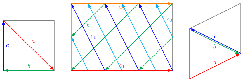
Refer to caption
Figure 8: Brane configuration for the three two-tori in Model 17 where the third two-torus is tilted. Fermion mass hierarchies result from the intersections on the second two-torus.
Table 9: The angles with respect to the orientifold plane made by the cycle wrapped by each stack of D-branes on each of the three two-tori in Model 17.

17θ1θ2θ3atan1(12)0π2b0tan1(12)tan1(2)ctan1(12)tan1(12)tan1(12)missing-subexpressionmissing-subexpressionmissing-subexpressionmissing-subexpression17superscript𝜃1superscript𝜃2superscript𝜃3missing-subexpressionmissing-subexpressionmissing-subexpressionmissing-subexpression𝑎superscript1120𝜋2missing-subexpressionmissing-subexpressionmissing-subexpressionmissing-subexpression𝑏0superscript112superscript12missing-subexpressionmissing-subexpressionmissing-subexpressionmissing-subexpression𝑐superscript112superscript112superscript112\begin{array}[]{|c|c|c|c|}\hline\cr\text{\hyperref@@ii[model17]{17}}&\theta^{1}&\theta^{2}&\theta^{3}\\ \hline\cr a&-\tan^{-1}\left(\frac{1}{\sqrt{2}}\right)&0&\frac{\pi}{2}\\ \hline\cr b&0&\tan^{-1}\left(\frac{1}{\sqrt{2}}\right)&-\tan^{-1}\left(\sqrt{2}\right)\\ \hline\cr c&\tan^{-1}\left(\frac{1}{\sqrt{2}}\right)&-\tan^{-1}\left(\frac{1}{\sqrt{2}}\right)&-\tan^{-1}\left(\frac{1}{\sqrt{2}}\right)\\ \hline\cr\end{array}

The complex structure moduli U𝑈U from (18) are,

{U1,U2,U3}subscript𝑈1subscript𝑈2subscript𝑈3\displaystyle\{U_{1},U_{2},U_{3}\} ={i2,i23,23(1+i2)},absent𝑖2𝑖23231𝑖2\displaystyle=\left\{\frac{i}{\sqrt{2}},\frac{i\sqrt{2}}{3},\frac{2}{3}\left(1+i\sqrt{2}\right)\right\}, (150)

and the corresponding u𝑢u-moduli and s𝑠s-modulus in supergravity basis from (19) are,

{u1,u2,u3}subscript𝑢1subscript𝑢2subscript𝑢3\displaystyle\{u_{1},u_{2},u_{3}\} ={eϕ4243π,3eϕ4224π,eϕ42243π},absentsuperscript𝑒subscriptitalic-ϕ4423𝜋3superscript𝑒subscriptitalic-ϕ4242𝜋superscript𝑒subscriptitalic-ϕ42423𝜋\displaystyle=\left\{\frac{e^{-\phi_{4}}}{\sqrt[4]{2}\sqrt{3}\pi},\frac{\sqrt{3}e^{-\phi_{4}}}{2\sqrt[4]{2}\pi},\frac{e^{-\phi_{4}}}{2\sqrt[4]{2}\sqrt{3}\pi}\right\},
s𝑠\displaystyle s =3eϕ4224π.absent3superscript𝑒subscriptitalic-ϕ4242𝜋\displaystyle=\frac{\sqrt{3}e^{-\phi_{4}}}{2\sqrt[4]{2}\pi}. (151)

Using (24) and the values from the table A23, the gauge kinetic function becomes,

{fa,fb,fc}subscript𝑓𝑎subscript𝑓𝑏subscript𝑓𝑐\displaystyle\{f_{a},f_{b},f_{c}\} ={33eϕ41624π,33eϕ4824π,33eϕ41624π},absent33superscript𝑒subscriptitalic-ϕ41642𝜋33superscript𝑒subscriptitalic-ϕ4842𝜋33superscript𝑒subscriptitalic-ϕ41642𝜋\displaystyle=\left\{\frac{3\sqrt{3}e^{-\phi_{4}}}{16\sqrt[4]{2}\pi},\frac{3\sqrt{3}e^{-\phi_{4}}}{8\sqrt[4]{2}\pi},\frac{3\sqrt{3}e^{-\phi_{4}}}{16\sqrt[4]{2}\pi}\right\}, (152)

To calculate gaugino masses M1,2,3subscript𝑀123M_{1,2,3} respectively for U(1)YUsubscript1𝑌{\rm U}(1)_{Y}, SU(2)LSUsubscript2𝐿{\rm SU}(2)_{L} and SU(3)cSUsubscript3𝑐{\rm SU}(3)_{c} gauge groups, we first compute Ma,b,csubscript𝑀𝑎𝑏𝑐M_{a,b,c} using (3.2) as,

Masubscript𝑀𝑎\displaystyle M_{a} =m3/2(Θ22Θ4)3,absentsubscript𝑚32subscriptΘ22subscriptΘ43\displaystyle=\frac{m_{3/2}(\Theta_{2}-2\Theta_{4})}{\sqrt{3}},
Mbsubscript𝑀𝑏\displaystyle M_{b} =m3/2(Θ12Θ4)3,absentsubscript𝑚32subscriptΘ12subscriptΘ43\displaystyle=\frac{m_{3/2}(\Theta_{1}-2\Theta_{4})}{\sqrt{3}},
Mcsubscript𝑀𝑐\displaystyle M_{c} =m3/2(Θ2+2Θ3)3.absentsubscript𝑚32subscriptΘ22subscriptΘ33\displaystyle=\frac{m_{3/2}(\Theta_{2}+2\Theta_{3})}{\sqrt{3}}. (153)

Next, to compute the trilinear coupling and the sleptons mass-squared we require the angles, the differences of angles and their first and second order derivatives with respect to the moduli. In table 9 we show the angles (44) made by the cycle wrapped by each stack D6 branes with respect to the orientifold plane. The differences of the angles, θxyiθyiθxisuperscriptsubscript𝜃𝑥𝑦𝑖superscriptsubscript𝜃𝑦𝑖superscriptsubscript𝜃𝑥𝑖\theta_{xy}^{i}\equiv\theta_{y}^{i}-\theta_{x}^{i} are,

[{0.,0.,0.}{0.242928,0.473887,0.230959}{0.186276,0.186276,0.0893668}{0.242928,0.473887,0.230959}{0.,0.,0.}{0.429204,0.287611,0.141593}{0.186276,0.186276,0.0893668}{0.429204,0.287611,0.141593}{0.,0.,0.}]\displaystyle\hskip-10.00002pt\left[\begin{array}[]{ccc}\{0.,0.,0.\}&\{-0.242928,0.473887,-0.230959\}&\{0.186276,0.186276,-0.0893668\}\\ \{0.242928,-0.473887,0.230959\}&\{0.,0.,0.\}&\{0.429204,-0.287611,0.141593\}\\ \{-0.186276,-0.186276,0.0893668\}&\{-0.429204,0.287611,-0.141593\}&\{0.,0.,0.\}\\ \end{array}\right] (157)

To account for the negative angle differences it is convenient to define the sign function σxyisuperscriptsubscript𝜎𝑥𝑦𝑖\sigma_{xy}^{i}, which is 11-1 only for negative angle difference and +11+1 otherwise,

σxyi(1)1H(θxyi)superscriptsubscript𝜎𝑥𝑦𝑖superscript11𝐻superscriptsubscript𝜃𝑥𝑦𝑖\displaystyle\sigma_{xy}^{i}\equiv(-1)^{1-H(\theta_{xy}^{i})} =({1,1,1}{1,1,1}{1,1,1}{1,1,1}{1,1,1}{1,1,1}{1,1,1}{1,1,1}{1,1,1}),absent111111111111111111111111111\displaystyle=\left(\begin{array}[]{ccc}\{1,1,1\}&\{-1,1,-1\}&\{1,1,-1\}\\ \{1,-1,1\}&\{1,1,1\}&\{1,-1,1\}\\ \{-1,-1,1\}&\{-1,1,-1\}&\{1,1,1\}\\ \end{array}\right), (161)

where H(x)𝐻𝑥H(x) is the unit step function. And the function ηxysubscript𝜂𝑥𝑦\eta_{xy} can thus be defined by taking the product on the torus index i𝑖i as,

ηxyiσxyi=(111111111).subscript𝜂𝑥𝑦subscriptproduct𝑖superscriptsubscript𝜎𝑥𝑦𝑖111111111\eta_{xy}\equiv\prod_{i}\sigma_{xy}^{i}=\left(\begin{array}[]{ccc}1&1&-1\\ -1&1&-1\\ 1&1&1\\ \end{array}\right). (162)

Using the values of σxyisuperscriptsubscript𝜎𝑥𝑦𝑖\sigma_{xy}^{i} and ηxyisuperscriptsubscript𝜂𝑥𝑦𝑖\eta_{xy}^{i} in (60) we can compute the four cases of functions Ψ(θxy)Ψsubscript𝜃𝑥𝑦\Psi(\theta_{xy}) defined in (55) and (56). Similarly we calculate the derivative Ψ(θxyj)=dΨ(θxyj)dθxyjsuperscriptΨsubscriptsuperscript𝜃𝑗𝑥𝑦𝑑Ψsubscriptsuperscript𝜃𝑗𝑥𝑦𝑑subscriptsuperscript𝜃𝑗𝑥𝑦\Psi^{\prime}(\theta^{j}_{xy})=\frac{d\Psi(\theta^{j}_{xy})}{d\theta^{j}_{xy}} using equations (63), (3.3), (3.3) and the properties of digamma function ψ(0)(z)superscript𝜓0𝑧\psi^{(0)}(z) (3.3) while neglecting the contribution of the t𝑡t-moduli.

Utilizing above results while ignoring the CP-violating phases γisubscript𝛾𝑖\gamma_{i}, the the gaugino masses for the respective gauge groups U(1)YUsubscript1𝑌{\rm U}(1)_{Y}, SU(2)LSUsubscript2𝐿{\rm SU}(2)_{L} and SU(3)CSUsubscript3𝐶{\rm SU}(3)_{C}; the trilinear coupling (3.2); and squared-masses of squarks and sleptons (3.2) are obtained as follows,

MB~subscript𝑀~𝐵\displaystyle M_{\tilde{B}} MY=m3/2(5Θ2+6Θ34Θ4)53,absentsubscript𝑀𝑌subscript𝑚325subscriptΘ26subscriptΘ34subscriptΘ453\displaystyle\equiv M_{Y}=\frac{m_{3/2}(5\Theta_{2}+6\Theta_{3}-4\Theta_{4})}{5\sqrt{3}},
MW~subscript𝑀~𝑊\displaystyle M_{\tilde{W}} Mb=m3/2(Θ12Θ4)3,absentsubscript𝑀𝑏subscript𝑚32subscriptΘ12subscriptΘ43\displaystyle\equiv M_{b}=\frac{m_{3/2}(\Theta_{1}-2\Theta_{4})}{\sqrt{3}},
Mg~subscript𝑀~𝑔\displaystyle M_{\tilde{g}} Ma=m3/2(Θ22Θ4)3,absentsubscript𝑀𝑎subscript𝑚32subscriptΘ22subscriptΘ43\displaystyle\equiv M_{a}=\frac{m_{3/2}(\Theta_{2}-2\Theta_{4})}{\sqrt{3}},
A0subscript𝐴0\displaystyle A_{0} Aabc=m3/2(0.128593Θ11.64721Θ20.107781Θ3+0.151538Θ4),absentsubscript𝐴𝑎𝑏𝑐subscript𝑚320.128593subscriptΘ11.64721subscriptΘ20.107781subscriptΘ30.151538subscriptΘ4\displaystyle\equiv A_{abc}=m_{3/2}\Bigl{(}-0.128593\Theta_{1}-1.64721\Theta_{2}-0.107781\Theta_{3}+0.151538\Theta_{4}\Bigr{)},
mL2mab2subscriptsuperscript𝑚2𝐿subscriptsuperscript𝑚2𝑎𝑏\displaystyle m^{2}_{L}\equiv m^{2}_{ab} =m3/22(0.36917Θ1+20.669259Θ1Θ20.840813Θ1Θ31.82443Θ1Θ4\displaystyle=m_{3/2}^{2}\Bigl{(}0.36917\Theta_{1}{}^{2}+0.669259\Theta_{1}\Theta_{2}-0.840813\Theta_{1}\Theta_{3}-1.82443\Theta_{1}\Theta_{4}
+0.375979Θ220.820669Θ2Θ30.733709Θ2Θ40.929866Θ32\displaystyle\quad+0.375979\Theta_{2}{}^{2}-0.820669\Theta_{2}\Theta_{3}-0.733709\Theta_{2}\Theta_{4}-0.929866\Theta_{3}{}^{2}
+1.7274Θ3Θ41.1538Θ4+21),\displaystyle\quad+1.7274\Theta_{3}\Theta_{4}-1.1538\Theta_{4}{}^{2}+1\Bigr{)},
mR2mac2subscriptsuperscript𝑚2𝑅subscriptsuperscript𝑚2𝑎𝑐\displaystyle m^{2}_{R}\equiv m^{2}_{ac} =m3/22(2.2278Θ122.22881Θ1Θ2+0.0357856Θ1Θ3+1.61629Θ1Θ4\displaystyle=m_{3/2}^{2}\Bigl{(}-2.2278\Theta_{1}{}^{2}-2.22881\Theta_{1}\Theta_{2}+0.0357856\Theta_{1}\Theta_{3}+1.61629\Theta_{1}\Theta_{4}
+0.395725Θ2+20.464088Θ2Θ3+0.503187Θ2Θ4+0.535193Θ32\displaystyle\quad+0.395725\Theta_{2}{}^{2}+0.464088\Theta_{2}\Theta_{3}+0.503187\Theta_{2}\Theta_{4}+0.535193\Theta_{3}{}^{2}
3.12602Θ3Θ4+0.309973Θ4+21).\displaystyle\quad-3.12602\Theta_{3}\Theta_{4}+0.309973\Theta_{4}{}^{2}+1\Bigr{)}. (163)

All soft terms are subject to the constraint (38).

4.8 Model 17-dual

In Model 17-dual the three-point Yukawa couplings arise from the triplet intersections from the branes a𝑎a, b𝑏b and c𝑐c on the second two-torus with 9 pairs of Higgs from the 𝒩=2𝒩2\mathcal{N}=2 sector. Yukawa matrices for the Model 17-dual are of rank 3 and the three intersections required to form the disk diagrams for the Yukawa couplings all occur on the second torus as shown in figure 9.
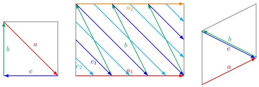
Refer to caption
Figure 9: Brane configuration for the three two-tori in Model 17-dual where the third two-torus is tilted. Fermion mass hierarchies result from the intersections on the second two-torus.
Table 10: The angles with respect to the orientifold plane made by the cycle wrapped by each stack of D-branes on each of the three two-tori in Model 17-dual.

17-dualθ1θ2θ3atan1(12)π20b0tan1(2)tan1(12)ctan1(12)tan1(12)tan1(12)missing-subexpressionmissing-subexpressionmissing-subexpressionmissing-subexpression17-dualsuperscript𝜃1superscript𝜃2superscript𝜃3missing-subexpressionmissing-subexpressionmissing-subexpressionmissing-subexpression𝑎superscript112𝜋20missing-subexpressionmissing-subexpressionmissing-subexpressionmissing-subexpression𝑏0superscript12superscript112missing-subexpressionmissing-subexpressionmissing-subexpressionmissing-subexpression𝑐superscript112superscript112superscript112\begin{array}[]{|c|c|c|c|}\hline\cr\text{\hyperref@@ii[model17.5]{17-dual}}&\theta^{1}&\theta^{2}&\theta^{3}\\ \hline\cr a&-\tan^{-1}\left(\frac{1}{\sqrt{2}}\right)&\frac{\pi}{2}&0\\ \hline\cr b&0&-\tan^{-1}\left(\sqrt{2}\right)&\tan^{-1}\left(\frac{1}{\sqrt{2}}\right)\\ \hline\cr c&\tan^{-1}\left(\frac{1}{\sqrt{2}}\right)&-\tan^{-1}\left(\frac{1}{\sqrt{2}}\right)&-\tan^{-1}\left(\frac{1}{\sqrt{2}}\right)\\ \hline\cr\end{array}

The complex structure moduli U𝑈U from (18) are,

{U1,U2,U3}subscript𝑈1subscript𝑈2subscript𝑈3\displaystyle\{U_{1},U_{2},U_{3}\} ={i2,i23,23(1+i2)},absent𝑖2𝑖23231𝑖2\displaystyle=\left\{\frac{i}{\sqrt{2}},\frac{i\sqrt{2}}{3},\frac{2}{3}\left(1+i\sqrt{2}\right)\right\}, (164)

and the corresponding u𝑢u-moduli and s𝑠s-modulus in supergravity basis from (19) are,

{u1,u2,u3}subscript𝑢1subscript𝑢2subscript𝑢3\displaystyle\{u_{1},u_{2},u_{3}\} ={eϕ4243π,3eϕ4224π,eϕ42243π},absentsuperscript𝑒subscriptitalic-ϕ4423𝜋3superscript𝑒subscriptitalic-ϕ4242𝜋superscript𝑒subscriptitalic-ϕ42423𝜋\displaystyle=\left\{\frac{e^{-\phi_{4}}}{\sqrt[4]{2}\sqrt{3}\pi},\frac{\sqrt{3}e^{-\phi_{4}}}{2\sqrt[4]{2}\pi},\frac{e^{-\phi_{4}}}{2\sqrt[4]{2}\sqrt{3}\pi}\right\},
s𝑠\displaystyle s =3eϕ4224π.absent3superscript𝑒subscriptitalic-ϕ4242𝜋\displaystyle=\frac{\sqrt{3}e^{-\phi_{4}}}{2\sqrt[4]{2}\pi}. (165)

Using (24) and the values from the table A24, the gauge kinetic function becomes,

{fa,fb,fc}subscript𝑓𝑎subscript𝑓𝑏subscript𝑓𝑐\displaystyle\{f_{a},f_{b},f_{c}\} ={33eϕ41624π,33eϕ41624π,33eϕ4824π},absent33superscript𝑒subscriptitalic-ϕ41642𝜋33superscript𝑒subscriptitalic-ϕ41642𝜋33superscript𝑒subscriptitalic-ϕ4842𝜋\displaystyle=\left\{\frac{3\sqrt{3}e^{-\phi_{4}}}{16\sqrt[4]{2}\pi},\frac{3\sqrt{3}e^{-\phi_{4}}}{16\sqrt[4]{2}\pi},\frac{3\sqrt{3}e^{-\phi_{4}}}{8\sqrt[4]{2}\pi}\right\}, (166)

To calculate gaugino masses M1,2,3subscript𝑀123M_{1,2,3} respectively for U(1)YUsubscript1𝑌{\rm U}(1)_{Y}, SU(2)LSUsubscript2𝐿{\rm SU}(2)_{L} and SU(3)cSUsubscript3𝑐{\rm SU}(3)_{c} gauge groups, we first compute Ma,b,csubscript𝑀𝑎𝑏𝑐M_{a,b,c} using (3.2) as,

Masubscript𝑀𝑎\displaystyle M_{a} =m3/2(Θ22Θ4)3,absentsubscript𝑚32subscriptΘ22subscriptΘ43\displaystyle=\frac{m_{3/2}(\Theta_{2}-2\Theta_{4})}{\sqrt{3}},
Mbsubscript𝑀𝑏\displaystyle M_{b} =m3/2(Θ2+2Θ3)3,absentsubscript𝑚32subscriptΘ22subscriptΘ33\displaystyle=\frac{m_{3/2}(\Theta_{2}+2\Theta_{3})}{\sqrt{3}},
Mcsubscript𝑀𝑐\displaystyle M_{c} =m3/2(Θ12Θ4)3.absentsubscript𝑚32subscriptΘ12subscriptΘ43\displaystyle=\frac{m_{3/2}(\Theta_{1}-2\Theta_{4})}{\sqrt{3}}. (167)

Next, to compute the trilinear coupling and the sleptons mass-squared we require the angles, the differences of angles and their first and second order derivatives with respect to the moduli. In table 10 we show the angles (44) made by the cycle wrapped by each stack D6 branes with respect to the orientifold plane. The differences of the angles, θxyiθyiθxisuperscriptsubscript𝜃𝑥𝑦𝑖superscriptsubscript𝜃𝑦𝑖superscriptsubscript𝜃𝑥𝑖\theta_{xy}^{i}\equiv\theta_{y}^{i}-\theta_{x}^{i} are,

[{0.,0.,0.}{0.186276,0.186276,0.0893668}{0.242928,0.473887,0.230959}{0.186276,0.186276,0.0893668}{0.,0.,0.}{0.429204,0.287611,0.141593}{0.242928,0.473887,0.230959}{0.429204,0.287611,0.141593}{0.,0.,0.}]\displaystyle\hskip-10.00002pt\left[\begin{array}[]{ccc}\{0.,0.,0.\}&\{0.186276,0.186276,-0.0893668\}&\{-0.242928,0.473887,-0.230959\}\\ \{-0.186276,-0.186276,0.0893668\}&\{0.,0.,0.\}&\{-0.429204,0.287611,-0.141593\}\\ \{0.242928,-0.473887,0.230959\}&\{0.429204,-0.287611,0.141593\}&\{0.,0.,0.\}\\ \end{array}\right] (171)

To account for the negative angle differences it is convenient to define the sign function σxyisuperscriptsubscript𝜎𝑥𝑦𝑖\sigma_{xy}^{i}, which is 11-1 only for negative angle difference and +11+1 otherwise,

σxyi(1)1H(θxyi)superscriptsubscript𝜎𝑥𝑦𝑖superscript11𝐻superscriptsubscript𝜃𝑥𝑦𝑖\displaystyle\sigma_{xy}^{i}\equiv(-1)^{1-H(\theta_{xy}^{i})} =({1,1,1}{1,1,1}{1,1,1}{1,1,1}{1,1,1}{1,1,1}{1,1,1}{1,1,1}{1,1,1}),absent111111111111111111111111111\displaystyle=\left(\begin{array}[]{ccc}\{1,1,1\}&\{1,1,-1\}&\{-1,1,-1\}\\ \{-1,-1,1\}&\{1,1,1\}&\{-1,1,-1\}\\ \{1,-1,1\}&\{1,-1,1\}&\{1,1,1\}\\ \end{array}\right), (175)

where H(x)𝐻𝑥H(x) is the unit step function. And the function ηxysubscript𝜂𝑥𝑦\eta_{xy} can thus be defined by taking the product on the torus index i𝑖i as,

ηxyiσxyi=(111111111).subscript𝜂𝑥𝑦subscriptproduct𝑖superscriptsubscript𝜎𝑥𝑦𝑖111111111\eta_{xy}\equiv\prod_{i}\sigma_{xy}^{i}=\left(\begin{array}[]{ccc}1&-1&1\\ 1&1&1\\ -1&-1&1\\ \end{array}\right). (176)

Using the values of σxyisuperscriptsubscript𝜎𝑥𝑦𝑖\sigma_{xy}^{i} and ηxyisuperscriptsubscript𝜂𝑥𝑦𝑖\eta_{xy}^{i} in (60) we can compute the four cases of functions Ψ(θxy)Ψsubscript𝜃𝑥𝑦\Psi(\theta_{xy}) defined in (55) and (56). Similarly we calculate the derivative Ψ(θxyj)=dΨ(θxyj)dθxyjsuperscriptΨsubscriptsuperscript𝜃𝑗𝑥𝑦𝑑Ψsubscriptsuperscript𝜃𝑗𝑥𝑦𝑑subscriptsuperscript𝜃𝑗𝑥𝑦\Psi^{\prime}(\theta^{j}_{xy})=\frac{d\Psi(\theta^{j}_{xy})}{d\theta^{j}_{xy}} using equations (63), (3.3), (3.3) and the properties of digamma function ψ(0)(z)superscript𝜓0𝑧\psi^{(0)}(z) (3.3) while neglecting the contribution of the t𝑡t-moduli.

Utilizing above results while ignoring the CP-violating phases γisubscript𝛾𝑖\gamma_{i}, the the gaugino masses for the respective gauge groups U(1)YUsubscript1𝑌{\rm U}(1)_{Y}, SU(2)LSUsubscript2𝐿{\rm SU}(2)_{L} and SU(3)CSUsubscript3𝐶{\rm SU}(3)_{C}; the trilinear coupling (3.2); and squared-masses of squarks and sleptons (3.2) are obtained as follows,

MB~subscript𝑀~𝐵\displaystyle M_{\tilde{B}} MY=m3/2(3Θ1+Θ28Θ4)43,absentsubscript𝑀𝑌subscript𝑚323subscriptΘ1subscriptΘ28subscriptΘ443\displaystyle\equiv M_{Y}=\frac{m_{3/2}(3\Theta_{1}+\Theta_{2}-8\Theta_{4})}{4\sqrt{3}},
MW~subscript𝑀~𝑊\displaystyle M_{\tilde{W}} Mb=m3/2(Θ2+2Θ3)3,absentsubscript𝑀𝑏subscript𝑚32subscriptΘ22subscriptΘ33\displaystyle\equiv M_{b}=\frac{m_{3/2}(\Theta_{2}+2\Theta_{3})}{\sqrt{3}},
Mg~subscript𝑀~𝑔\displaystyle M_{\tilde{g}} Ma=m3/2(Θ22Θ4)3,absentsubscript𝑀𝑎subscript𝑚32subscriptΘ22subscriptΘ43\displaystyle\equiv M_{a}=\frac{m_{3/2}(\Theta_{2}-2\Theta_{4})}{\sqrt{3}},
A0subscript𝐴0\displaystyle A_{0} Aabc=m3/2(0.128593Θ11.64721Θ20.107781Θ3+0.151538Θ4),absentsubscript𝐴𝑎𝑏𝑐subscript𝑚320.128593subscriptΘ11.64721subscriptΘ20.107781subscriptΘ30.151538subscriptΘ4\displaystyle\equiv A_{abc}=m_{3/2}\Bigl{(}-0.128593\Theta_{1}-1.64721\Theta_{2}-0.107781\Theta_{3}+0.151538\Theta_{4}\Bigr{)},
mL2mab2subscriptsuperscript𝑚2𝐿subscriptsuperscript𝑚2𝑎𝑏\displaystyle m^{2}_{L}\equiv m^{2}_{ab} =m3/22(2.2278Θ122.22881Θ1Θ2+0.0357856Θ1Θ3+1.61629Θ1Θ4\displaystyle=m_{3/2}^{2}\Bigl{(}-2.2278\Theta_{1}{}^{2}-2.22881\Theta_{1}\Theta_{2}+0.0357856\Theta_{1}\Theta_{3}+1.61629\Theta_{1}\Theta_{4}
+0.395725Θ2+20.464088Θ2Θ3+0.503187Θ2Θ4+0.535193Θ32\displaystyle\quad+0.395725\Theta_{2}{}^{2}+0.464088\Theta_{2}\Theta_{3}+0.503187\Theta_{2}\Theta_{4}+0.535193\Theta_{3}{}^{2}
3.12602Θ3Θ4+0.309973Θ4+21),\displaystyle\quad-3.12602\Theta_{3}\Theta_{4}+0.309973\Theta_{4}{}^{2}+1\Bigr{)},
mR2mac2subscriptsuperscript𝑚2𝑅subscriptsuperscript𝑚2𝑎𝑐\displaystyle m^{2}_{R}\equiv m^{2}_{ac} =m3/22(0.36917Θ1+20.669259Θ1Θ20.840813Θ1Θ31.82443Θ1Θ4\displaystyle=m_{3/2}^{2}\Bigl{(}0.36917\Theta_{1}{}^{2}+0.669259\Theta_{1}\Theta_{2}-0.840813\Theta_{1}\Theta_{3}-1.82443\Theta_{1}\Theta_{4}
+0.375979Θ220.820669Θ2Θ30.733709Θ2Θ40.929866Θ32\displaystyle\quad+0.375979\Theta_{2}{}^{2}-0.820669\Theta_{2}\Theta_{3}-0.733709\Theta_{2}\Theta_{4}-0.929866\Theta_{3}{}^{2}
+1.7274Θ3Θ41.1538Θ4+21).\displaystyle\quad+1.7274\Theta_{3}\Theta_{4}-1.1538\Theta_{4}{}^{2}+1\Bigr{)}. (177)

All soft terms are subject to the constraint (38).

4.9 Model 18

In Model 18 the three-point Yukawa couplings arise from the triplet intersections from the branes a𝑎a, b𝑏b and c𝑐c on the first two-torus with 9 pairs of Higgs from the 𝒩=2𝒩2\mathcal{N}=2 sector. Yukawa matrices for the Model 18 are of rank 3 and the three intersections required to form the disk diagrams for the Yukawa couplings all occur on the first torus as shown in figure 10.

Refer to caption
Figure 10: Brane configuration for the three two-tori in Model 18 where the third two-torus is tilted. Fermion mass hierarchies result from the intersections on the first two-torus.
Table 11: The angles with respect to the orientifold plane made by the cycle wrapped by each stack of D-branes on each of the three two-tori in Model 18.

18θ1θ2θ3atan1(12)tan1(2)tan1(14)b0π2tan1(29)ctan1(12)tan1(12)tan1(12)missing-subexpressionmissing-subexpressionmissing-subexpressionmissing-subexpression18superscript𝜃1superscript𝜃2superscript𝜃3missing-subexpressionmissing-subexpressionmissing-subexpressionmissing-subexpression𝑎superscript112superscript12superscript114missing-subexpressionmissing-subexpressionmissing-subexpressionmissing-subexpression𝑏0𝜋2superscript129missing-subexpressionmissing-subexpressionmissing-subexpressionmissing-subexpression𝑐superscript112superscript112superscript112\begin{array}[]{|c|c|c|c|}\hline\cr\text{\hyperref@@ii[model18]{18}}&\theta^{1}&\theta^{2}&\theta^{3}\\ \hline\cr a&-\tan^{-1}\left(\frac{1}{2}\right)&-\tan^{-1}(2)&\tan^{-1}\left(\frac{1}{4}\right)\\ \hline\cr b&0&\frac{\pi}{2}&\tan^{-1}\left(\frac{2}{9}\right)\\ \hline\cr c&\tan^{-1}\left(\frac{1}{2}\right)&-\tan^{-1}\left(\frac{1}{2}\right)&-\tan^{-1}\left(\frac{1}{2}\right)\\ \hline\cr\end{array}

The complex structure moduli U𝑈U from (18) are,

{U1,U2,U3}subscript𝑈1subscript𝑈2subscript𝑈3\displaystyle\{U_{1},U_{2},U_{3}\} ={i2,2i9,25+4i5},absent𝑖22𝑖9254𝑖5\displaystyle=\left\{\frac{i}{2},\frac{2i}{9},\frac{2}{5}+\frac{4i}{5}\right\}, (178)

and the corresponding u𝑢u-moduli and s𝑠s-modulus in supergravity basis from (19) are,

{u1,u2,u3}subscript𝑢1subscript𝑢2subscript𝑢3\displaystyle\{u_{1},u_{2},u_{3}\} ={eϕ43π,3eϕ44π,eϕ46π},absentsuperscript𝑒subscriptitalic-ϕ43𝜋3superscript𝑒subscriptitalic-ϕ44𝜋superscript𝑒subscriptitalic-ϕ46𝜋\displaystyle=\left\{\frac{e^{-\phi_{4}}}{3\pi},\frac{3e^{-\phi_{4}}}{4\pi},\frac{e^{-\phi_{4}}}{6\pi}\right\},
s𝑠\displaystyle s =3eϕ42π.absent3superscript𝑒subscriptitalic-ϕ42𝜋\displaystyle=\frac{3e^{-\phi_{4}}}{2\pi}. (179)

Using (24) and the values from the table A25, the gauge kinetic function becomes,

{fa,fb,fc}subscript𝑓𝑎subscript𝑓𝑏subscript𝑓𝑐\displaystyle\{f_{a},f_{b},f_{c}\} ={15eϕ432π,5eϕ424π,85eϕ496π},absent15superscript𝑒subscriptitalic-ϕ432𝜋5superscript𝑒subscriptitalic-ϕ424𝜋85superscript𝑒subscriptitalic-ϕ496𝜋\displaystyle=\left\{\frac{15e^{-\phi_{4}}}{32\pi},\frac{5e^{-\phi_{4}}}{24\pi},\frac{85e^{-\phi_{4}}}{96\pi}\right\}, (180)

To calculate gaugino masses M1,2,3subscript𝑀123M_{1,2,3} respectively for U(1)YUsubscript1𝑌{\rm U}(1)_{Y}, SU(2)LSUsubscript2𝐿{\rm SU}(2)_{L} and SU(3)cSUsubscript3𝑐{\rm SU}(3)_{c} gauge groups, we first compute Ma,b,csubscript𝑀𝑎𝑏𝑐M_{a,b,c} using (3.2) as,

Masubscript𝑀𝑎\displaystyle M_{a} =153m3/2(Θ24Θ4),absent153subscript𝑚32subscriptΘ24subscriptΘ4\displaystyle=\frac{1}{5}\sqrt{3}m_{3/2}(\Theta_{2}-4\Theta_{4}),
Mbsubscript𝑀𝑏\displaystyle M_{b} =153m3/2(Θ1+4Θ3),absent153subscript𝑚32subscriptΘ14subscriptΘ3\displaystyle=\frac{1}{5}\sqrt{3}m_{3/2}(\Theta_{1}+4\Theta_{3}),
Mcsubscript𝑀𝑐\displaystyle M_{c} =1853m3/2(8Θ1+9Θ24(Θ3+18Θ4)).absent1853subscript𝑚328subscriptΘ19subscriptΘ24subscriptΘ318subscriptΘ4\displaystyle=\frac{1}{85}\sqrt{3}m_{3/2}(8\Theta_{1}+9\Theta_{2}-4(\Theta_{3}+18\Theta_{4})). (181)

Next, to compute the trilinear coupling and the sleptons mass-squared we require the angles, the differences of angles and their first and second order derivatives with respect to the moduli. In table 11 we show the angles (44) made by the cycle wrapped by each stack D6 branes with respect to the orientifold plane. The differences of the angles, θxyiθyiθxisuperscriptsubscript𝜃𝑥𝑦𝑖superscriptsubscript𝜃𝑦𝑖superscriptsubscript𝜃𝑥𝑖\theta_{xy}^{i}\equiv\theta_{y}^{i}-\theta_{x}^{i} are,

[{0.,0.,0.}{0.501908,0.570796,0.214297}{0.291374,0.218669,0.0727048}{0.501908,0.570796,0.214297}{0.,0.,0.}{0.210535,0.352127,0.141593}{0.291374,0.218669,0.0727048}{0.210535,0.352127,0.141593}{0.,0.,0.}]\displaystyle\hskip-10.00002pt\left[\begin{array}[]{ccc}\{0.,0.,0.\}&\{-0.501908,0.570796,0.214297\}&\{-0.291374,0.218669,0.0727048\}\\ \{0.501908,-0.570796,-0.214297\}&\{0.,0.,0.\}&\{0.210535,-0.352127,-0.141593\}\\ \{0.291374,-0.218669,-0.0727048\}&\{-0.210535,0.352127,0.141593\}&\{0.,0.,0.\}\\ \end{array}\right] (185)

To account for the negative angle differences it is convenient to define the sign function σxyisuperscriptsubscript𝜎𝑥𝑦𝑖\sigma_{xy}^{i}, which is 11-1 only for negative angle difference and +11+1 otherwise,

σxyi(1)1H(θxyi)superscriptsubscript𝜎𝑥𝑦𝑖superscript11𝐻superscriptsubscript𝜃𝑥𝑦𝑖\displaystyle\sigma_{xy}^{i}\equiv(-1)^{1-H(\theta_{xy}^{i})} =({1,1,1}{1,1,1}{1,1,1}{1,1,1}{1,1,1}{1,1,1}{1,1,1}{1,1,1}{1,1,1}),absent111111111111111111111111111\displaystyle=\left(\begin{array}[]{ccc}\{1,1,1\}&\{-1,1,1\}&\{-1,1,1\}\\ \{1,-1,-1\}&\{1,1,1\}&\{1,-1,-1\}\\ \{1,-1,-1\}&\{-1,1,1\}&\{1,1,1\}\\ \end{array}\right), (189)

where H(x)𝐻𝑥H(x) is the unit step function. And the function ηxysubscript𝜂𝑥𝑦\eta_{xy} can thus be defined by taking the product on the torus index i𝑖i as,

ηxyiσxyi=(111111111).subscript𝜂𝑥𝑦subscriptproduct𝑖superscriptsubscript𝜎𝑥𝑦𝑖111111111\eta_{xy}\equiv\prod_{i}\sigma_{xy}^{i}=\left(\begin{array}[]{ccc}1&-1&-1\\ 1&1&1\\ 1&-1&1\\ \end{array}\right). (190)

Using the values of σxyisuperscriptsubscript𝜎𝑥𝑦𝑖\sigma_{xy}^{i} and ηxyisuperscriptsubscript𝜂𝑥𝑦𝑖\eta_{xy}^{i} in (60) we can compute the four cases of functions Ψ(θxy)Ψsubscript𝜃𝑥𝑦\Psi(\theta_{xy}) defined in (55) and (56). Similarly we calculate the derivative Ψ(θxyj)=dΨ(θxyj)dθxyjsuperscriptΨsubscriptsuperscript𝜃𝑗𝑥𝑦𝑑Ψsubscriptsuperscript𝜃𝑗𝑥𝑦𝑑subscriptsuperscript𝜃𝑗𝑥𝑦\Psi^{\prime}(\theta^{j}_{xy})=\frac{d\Psi(\theta^{j}_{xy})}{d\theta^{j}_{xy}} using equations (63), (3.3), (3.3) and the properties of digamma function ψ(0)(z)superscript𝜓0𝑧\psi^{(0)}(z) (3.3) while neglecting the contribution of the t𝑡t-moduli.

Utilizing above results while ignoring the CP-violating phases γisubscript𝛾𝑖\gamma_{i}, the the gaugino masses for the respective gauge groups U(1)YUsubscript1𝑌{\rm U}(1)_{Y}, SU(2)LSUsubscript2𝐿{\rm SU}(2)_{L} and SU(3)CSUsubscript3𝐶{\rm SU}(3)_{C}; the trilinear coupling (3.2); and squared-masses of squarks and sleptons (3.2) are obtained as follows,

MB~subscript𝑀~𝐵\displaystyle M_{\tilde{B}} MY=11153m3/2(8Θ1+15Θ24(Θ3+24Θ4)),absentsubscript𝑀𝑌11153subscript𝑚328subscriptΘ115subscriptΘ24subscriptΘ324subscriptΘ4\displaystyle\equiv M_{Y}=\frac{1}{115}\sqrt{3}m_{3/2}(8\Theta_{1}+15\Theta_{2}-4(\Theta_{3}+24\Theta_{4})),
MW~subscript𝑀~𝑊\displaystyle M_{\tilde{W}} Mb=153m3/2(Θ1+4Θ3),absentsubscript𝑀𝑏153subscript𝑚32subscriptΘ14subscriptΘ3\displaystyle\equiv M_{b}=\frac{1}{5}\sqrt{3}m_{3/2}(\Theta_{1}+4\Theta_{3}),
Mg~subscript𝑀~𝑔\displaystyle M_{\tilde{g}} Ma=153m3/2(Θ24Θ4),absentsubscript𝑀𝑎153subscript𝑚32subscriptΘ24subscriptΘ4\displaystyle\equiv M_{a}=\frac{1}{5}\sqrt{3}m_{3/2}(\Theta_{2}-4\Theta_{4}),
A0subscript𝐴0\displaystyle A_{0} Aabc=m3/2(1.82708Θ11.50614Θ2+1.42587Θ3+0.175299Θ4),absentsubscript𝐴𝑎𝑏𝑐subscript𝑚321.82708subscriptΘ11.50614subscriptΘ21.42587subscriptΘ30.175299subscriptΘ4\displaystyle\equiv A_{abc}=m_{3/2}\Bigl{(}-1.82708\Theta_{1}-1.50614\Theta_{2}+1.42587\Theta_{3}+0.175299\Theta_{4}\Bigr{)},
mL2mab2subscriptsuperscript𝑚2𝐿subscriptsuperscript𝑚2𝑎𝑏\displaystyle m^{2}_{L}\equiv m^{2}_{ab} =m3/22(0.730534Θ1+20.131797Θ1Θ21.01748Θ1Θ31.17062Θ1Θ4\displaystyle=m_{3/2}^{2}\Bigl{(}0.730534\Theta_{1}{}^{2}+0.131797\Theta_{1}\Theta_{2}-1.01748\Theta_{1}\Theta_{3}-1.17062\Theta_{1}\Theta_{4}
+0.144867Θ221.16345Θ2Θ30.752402Θ2Θ40.846416Θ32\displaystyle\quad+0.144867\Theta_{2}{}^{2}-1.16345\Theta_{2}\Theta_{3}-0.752402\Theta_{2}\Theta_{4}-0.846416\Theta_{3}{}^{2}
+0.832553Θ3Θ40.848056Θ4+21),\displaystyle\quad+0.832553\Theta_{3}\Theta_{4}-0.848056\Theta_{4}{}^{2}+1\Bigr{)},
mR2mac2subscriptsuperscript𝑚2𝑅subscriptsuperscript𝑚2𝑎𝑐\displaystyle m^{2}_{R}\equiv m^{2}_{ac} =m3/22(0.72924Θ1+20.0000979797Θ1Θ20.60321Θ1Θ32.56141Θ1Θ4\displaystyle=m_{3/2}^{2}\Bigl{(}0.72924\Theta_{1}{}^{2}+0.0000979797\Theta_{1}\Theta_{2}-0.60321\Theta_{1}\Theta_{3}-2.56141\Theta_{1}\Theta_{4}
+0.759033Θ222.39659Θ2Θ30.388307Θ2Θ41.82808Θ32\displaystyle\quad+0.759033\Theta_{2}{}^{2}-2.39659\Theta_{2}\Theta_{3}-0.388307\Theta_{2}\Theta_{4}-1.82808\Theta_{3}{}^{2}
+1.44981Θ3Θ4+0.339613Θ4+21).\displaystyle\quad+1.44981\Theta_{3}\Theta_{4}+0.339613\Theta_{4}{}^{2}+1\Bigr{)}. (191)

All soft terms are subject to the constraint (38).

4.10 Model 18-dual

In Model 18-dual the three-point Yukawa couplings arise from the triplet intersections from the branes a𝑎a, b𝑏b and c𝑐c on the first two-torus with 9 pairs of Higgs from the 𝒩=2𝒩2\mathcal{N}=2 sector. Yukawa matrices for the Model 18-dual are of rank 3 and the three intersections required to form the disk diagrams for the Yukawa couplings all occur on the first torus as shown in figure 11.

Refer to caption
Figure 11: Brane configuration for the three two-tori in Model 18-dual where the third two-torus is tilted. Fermion mass hierarchies result from the intersections on the first two-torus.
Table 12: The angles with respect to the orientifold plane made by the cycle wrapped by each stack of D-branes on each of the three two-tori in Model 18-dual.

18-dualθ1θ2θ3atan1(12)tan1(14)tan1(2)b0tan1(29)π2ctan1(12)tan1(12)tan1(12)missing-subexpressionmissing-subexpressionmissing-subexpressionmissing-subexpression18-dualsuperscript𝜃1superscript𝜃2superscript𝜃3missing-subexpressionmissing-subexpressionmissing-subexpressionmissing-subexpression𝑎superscript112superscript114superscript12missing-subexpressionmissing-subexpressionmissing-subexpressionmissing-subexpression𝑏0superscript129𝜋2missing-subexpressionmissing-subexpressionmissing-subexpressionmissing-subexpression𝑐superscript112superscript112superscript112\begin{array}[]{|c|c|c|c|}\hline\cr\text{\hyperref@@ii[model18.5]{18-dual}}&\theta^{1}&\theta^{2}&\theta^{3}\\ \hline\cr a&-\tan^{-1}\left(\frac{1}{2}\right)&\tan^{-1}\left(\frac{1}{4}\right)&-\tan^{-1}(2)\\ \hline\cr b&0&\tan^{-1}\left(\frac{2}{9}\right)&\frac{\pi}{2}\\ \hline\cr c&\tan^{-1}\left(\frac{1}{2}\right)&-\tan^{-1}\left(\frac{1}{2}\right)&-\tan^{-1}\left(\frac{1}{2}\right)\\ \hline\cr\end{array}

The complex structure moduli U𝑈U from (18) are,

{U1,U2,U3}subscript𝑈1subscript𝑈2subscript𝑈3\displaystyle\{U_{1},U_{2},U_{3}\} ={i2,2i9,25+4i5},absent𝑖22𝑖9254𝑖5\displaystyle=\left\{\frac{i}{2},\frac{2i}{9},\frac{2}{5}+\frac{4i}{5}\right\}, (192)

and the corresponding u𝑢u-moduli and s𝑠s-modulus in supergravity basis from (19) are,

{u1,u2,u3}subscript𝑢1subscript𝑢2subscript𝑢3\displaystyle\{u_{1},u_{2},u_{3}\} ={eϕ43π,3eϕ44π,eϕ46π},absentsuperscript𝑒subscriptitalic-ϕ43𝜋3superscript𝑒subscriptitalic-ϕ44𝜋superscript𝑒subscriptitalic-ϕ46𝜋\displaystyle=\left\{\frac{e^{-\phi_{4}}}{3\pi},\frac{3e^{-\phi_{4}}}{4\pi},\frac{e^{-\phi_{4}}}{6\pi}\right\},
s𝑠\displaystyle s =3eϕ42π.absent3superscript𝑒subscriptitalic-ϕ42𝜋\displaystyle=\frac{3e^{-\phi_{4}}}{2\pi}. (193)

Using (24) and the values from the table A26, the gauge kinetic function becomes,

{fa,fb,fc}subscript𝑓𝑎subscript𝑓𝑏subscript𝑓𝑐\displaystyle\{f_{a},f_{b},f_{c}\} ={15eϕ432π,85eϕ496π,5eϕ424π},absent15superscript𝑒subscriptitalic-ϕ432𝜋85superscript𝑒subscriptitalic-ϕ496𝜋5superscript𝑒subscriptitalic-ϕ424𝜋\displaystyle=\left\{\frac{15e^{-\phi_{4}}}{32\pi},\frac{85e^{-\phi_{4}}}{96\pi},\frac{5e^{-\phi_{4}}}{24\pi}\right\}, (194)

To calculate gaugino masses M1,2,3subscript𝑀123M_{1,2,3} respectively for U(1)YUsubscript1𝑌{\rm U}(1)_{Y}, SU(2)LSUsubscript2𝐿{\rm SU}(2)_{L} and SU(3)cSUsubscript3𝑐{\rm SU}(3)_{c} gauge groups, we first compute Ma,b,csubscript𝑀𝑎𝑏𝑐M_{a,b,c} using (3.2) as,

Masubscript𝑀𝑎\displaystyle M_{a} =153m3/2(Θ24Θ4),absent153subscript𝑚32subscriptΘ24subscriptΘ4\displaystyle=\frac{1}{5}\sqrt{3}m_{3/2}(\Theta_{2}-4\Theta_{4}),
Mbsubscript𝑀𝑏\displaystyle M_{b} =1853m3/2(8Θ1+9Θ24(Θ3+18Θ4)),absent1853subscript𝑚328subscriptΘ19subscriptΘ24subscriptΘ318subscriptΘ4\displaystyle=\frac{1}{85}\sqrt{3}m_{3/2}(8\Theta_{1}+9\Theta_{2}-4(\Theta_{3}+18\Theta_{4})),
Mcsubscript𝑀𝑐\displaystyle M_{c} =153m3/2(Θ1+4Θ3).absent153subscript𝑚32subscriptΘ14subscriptΘ3\displaystyle=\frac{1}{5}\sqrt{3}m_{3/2}(\Theta_{1}+4\Theta_{3}). (195)

Next, to compute the trilinear coupling and the sleptons mass-squared we require the angles, the differences of angles and their first and second order derivatives with respect to the moduli. In table 12 we show the angles (44) made by the cycle wrapped by each stack D6 branes with respect to the orientifold plane. The differences of the angles, θxyiθyiθxisuperscriptsubscript𝜃𝑥𝑦𝑖superscriptsubscript𝜃𝑦𝑖superscriptsubscript𝜃𝑥𝑖\theta_{xy}^{i}\equiv\theta_{y}^{i}-\theta_{x}^{i} are,

[{0.,0.,0.}{0.291374,0.218669,0.0727048}{0.501908,0.570796,0.214297}{0.291374,0.218669,0.0727048}{0.,0.,0.}{0.210535,0.352127,0.141593}{0.501908,0.570796,0.214297}{0.210535,0.352127,0.141593}{0.,0.,0.}]\displaystyle\hskip-10.00002pt\left[\begin{array}[]{ccc}\{0.,0.,0.\}&\{-0.291374,0.218669,0.0727048\}&\{-0.501908,0.570796,0.214297\}\\ \{0.291374,-0.218669,-0.0727048\}&\{0.,0.,0.\}&\{-0.210535,0.352127,0.141593\}\\ \{0.501908,-0.570796,-0.214297\}&\{0.210535,-0.352127,-0.141593\}&\{0.,0.,0.\}\\ \end{array}\right] (199)

To account for the negative angle differences it is convenient to define the sign function σxyisuperscriptsubscript𝜎𝑥𝑦𝑖\sigma_{xy}^{i}, which is 11-1 only for negative angle difference and +11+1 otherwise,

σxyi(1)1H(θxyi)superscriptsubscript𝜎𝑥𝑦𝑖superscript11𝐻superscriptsubscript𝜃𝑥𝑦𝑖\displaystyle\sigma_{xy}^{i}\equiv(-1)^{1-H(\theta_{xy}^{i})} =({1,1,1}{1,1,1}{1,1,1}{1,1,1}{1,1,1}{1,1,1}{1,1,1}{1,1,1}{1,1,1}),absent111111111111111111111111111\displaystyle=\left(\begin{array}[]{ccc}\{1,1,1\}&\{-1,1,1\}&\{-1,1,1\}\\ \{1,-1,-1\}&\{1,1,1\}&\{-1,1,1\}\\ \{1,-1,-1\}&\{1,-1,-1\}&\{1,1,1\}\\ \end{array}\right), (203)

where H(x)𝐻𝑥H(x) is the unit step function. And the function ηxysubscript𝜂𝑥𝑦\eta_{xy} can thus be defined by taking the product on the torus index i𝑖i as,

ηxyiσxyi=(111111111).subscript𝜂𝑥𝑦subscriptproduct𝑖superscriptsubscript𝜎𝑥𝑦𝑖111111111\eta_{xy}\equiv\prod_{i}\sigma_{xy}^{i}=\left(\begin{array}[]{ccc}1&-1&-1\\ 1&1&-1\\ 1&1&1\\ \end{array}\right). (204)

Using the values of σxyisuperscriptsubscript𝜎𝑥𝑦𝑖\sigma_{xy}^{i} and ηxyisuperscriptsubscript𝜂𝑥𝑦𝑖\eta_{xy}^{i} in (60) we can compute the four cases of functions Ψ(θxy)Ψsubscript𝜃𝑥𝑦\Psi(\theta_{xy}) defined in (55) and (56). Similarly we calculate the derivative Ψ(θxyj)=dΨ(θxyj)dθxyjsuperscriptΨsubscriptsuperscript𝜃𝑗𝑥𝑦𝑑Ψsubscriptsuperscript𝜃𝑗𝑥𝑦𝑑subscriptsuperscript𝜃𝑗𝑥𝑦\Psi^{\prime}(\theta^{j}_{xy})=\frac{d\Psi(\theta^{j}_{xy})}{d\theta^{j}_{xy}} using equations (63), (3.3), (3.3) and the properties of digamma function ψ(0)(z)superscript𝜓0𝑧\psi^{(0)}(z) (3.3) while neglecting the contribution of the t𝑡t-moduli.

Utilizing above results while ignoring the CP-violating phases γisubscript𝛾𝑖\gamma_{i}, the the gaugino masses for the respective gauge groups U(1)YUsubscript1𝑌{\rm U}(1)_{Y}, SU(2)LSUsubscript2𝐿{\rm SU}(2)_{L} and SU(3)CSUsubscript3𝐶{\rm SU}(3)_{C}; the trilinear coupling (3.2); and squared-masses of squarks and sleptons (3.2) are obtained as follows,

MB~subscript𝑀~𝐵\displaystyle M_{\tilde{B}} MY=1253m3/2(2Θ1+3Θ2+8Θ312Θ4),absentsubscript𝑀𝑌1253subscript𝑚322subscriptΘ13subscriptΘ28subscriptΘ312subscriptΘ4\displaystyle\equiv M_{Y}=\frac{1}{25}\sqrt{3}m_{3/2}(2\Theta_{1}+3\Theta_{2}+8\Theta_{3}-12\Theta_{4}),
MW~subscript𝑀~𝑊\displaystyle M_{\tilde{W}} Mb=1853m3/2(8Θ1+9Θ24(Θ3+18Θ4)),absentsubscript𝑀𝑏1853subscript𝑚328subscriptΘ19subscriptΘ24subscriptΘ318subscriptΘ4\displaystyle\equiv M_{b}=\frac{1}{85}\sqrt{3}m_{3/2}(8\Theta_{1}+9\Theta_{2}-4(\Theta_{3}+18\Theta_{4})),
Mg~subscript𝑀~𝑔\displaystyle M_{\tilde{g}} Ma=153m3/2(Θ24Θ4),absentsubscript𝑀𝑎153subscript𝑚32subscriptΘ24subscriptΘ4\displaystyle\equiv M_{a}=\frac{1}{5}\sqrt{3}m_{3/2}(\Theta_{2}-4\Theta_{4}),
A0subscript𝐴0\displaystyle A_{0} Aabc=m3/2(1.82708Θ11.50614Θ2+1.42587Θ3+0.175299Θ4),absentsubscript𝐴𝑎𝑏𝑐subscript𝑚321.82708subscriptΘ11.50614subscriptΘ21.42587subscriptΘ30.175299subscriptΘ4\displaystyle\equiv A_{abc}=m_{3/2}\Bigl{(}-1.82708\Theta_{1}-1.50614\Theta_{2}+1.42587\Theta_{3}+0.175299\Theta_{4}\Bigr{)},
mL2mab2subscriptsuperscript𝑚2𝐿subscriptsuperscript𝑚2𝑎𝑏\displaystyle m^{2}_{L}\equiv m^{2}_{ab} =m3/22(0.72924Θ1+20.0000979797Θ1Θ20.60321Θ1Θ32.56141Θ1Θ4\displaystyle=m_{3/2}^{2}\Bigl{(}0.72924\Theta_{1}{}^{2}+0.0000979797\Theta_{1}\Theta_{2}-0.60321\Theta_{1}\Theta_{3}-2.56141\Theta_{1}\Theta_{4}
+0.759033Θ222.39659Θ2Θ30.388307Θ2Θ41.82808Θ32\displaystyle\quad+0.759033\Theta_{2}{}^{2}-2.39659\Theta_{2}\Theta_{3}-0.388307\Theta_{2}\Theta_{4}-1.82808\Theta_{3}{}^{2}
+1.44981Θ3Θ4+0.339613Θ4+21),\displaystyle\quad+1.44981\Theta_{3}\Theta_{4}+0.339613\Theta_{4}{}^{2}+1\Bigr{)},
mR2mac2subscriptsuperscript𝑚2𝑅subscriptsuperscript𝑚2𝑎𝑐\displaystyle m^{2}_{R}\equiv m^{2}_{ac} =m3/22(0.730534Θ1+20.131797Θ1Θ21.01748Θ1Θ31.17062Θ1Θ4\displaystyle=m_{3/2}^{2}\Bigl{(}0.730534\Theta_{1}{}^{2}+0.131797\Theta_{1}\Theta_{2}-1.01748\Theta_{1}\Theta_{3}-1.17062\Theta_{1}\Theta_{4}
+0.144867Θ221.16345Θ2Θ30.752402Θ2Θ40.846416Θ32\displaystyle\quad+0.144867\Theta_{2}{}^{2}-1.16345\Theta_{2}\Theta_{3}-0.752402\Theta_{2}\Theta_{4}-0.846416\Theta_{3}{}^{2}
+0.832553Θ3Θ40.848056Θ4+21).\displaystyle\quad+0.832553\Theta_{3}\Theta_{4}-0.848056\Theta_{4}{}^{2}+1\Bigr{)}. (205)

All soft terms are subject to the constraint (38).

4.11 Model 19

In Model 19 the three-point Yukawa couplings arise from the triplet intersections from the branes a𝑎a, b𝑏b and c𝑐c on the first two-torus with 9 pairs of Higgs from the 𝒩=2𝒩2\mathcal{N}=2 sector. Yukawa matrices for the Model 19 are of rank 3 and the three intersections required to form the disk diagrams for the Yukawa couplings all occur on the first torus as shown in figure 12.
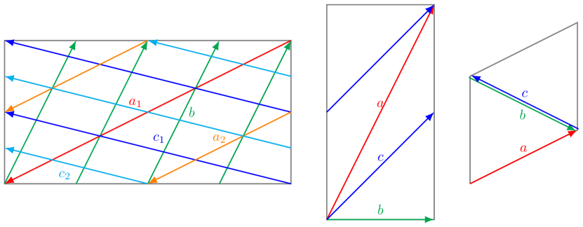
Refer to caption
Figure 12: Brane configuration for the three two-tori in Model 19 where the third two-torus is tilted. Fermion mass hierarchies result from the intersections on the first two-torus.
Table 13: The angles with respect to the orientifold plane made by the cycle wrapped by each stack of D-branes on each of the three two-tori in Model 19.

19θ1θ2θ3atan1(723)tan1(4723)tan1(7232)btan1(161)0tan1(1612)ctan1(4723)tan1(4723)tan1(4723)missing-subexpressionmissing-subexpressionmissing-subexpressionmissing-subexpression19superscript𝜃1superscript𝜃2superscript𝜃3missing-subexpressionmissing-subexpressionmissing-subexpressionmissing-subexpression𝑎superscript1723superscript14723superscript17232missing-subexpressionmissing-subexpressionmissing-subexpressionmissing-subexpression𝑏superscript11610superscript11612missing-subexpressionmissing-subexpressionmissing-subexpressionmissing-subexpression𝑐superscript14723superscript14723superscript14723\begin{array}[]{|c|c|c|c|}\hline\cr\text{\hyperref@@ii[model19]{19}}&\theta^{1}&\theta^{2}&\theta^{3}\\ \hline\cr a&\tan^{-1}\left(\sqrt{\frac{7}{23}}\right)&\tan^{-1}\left(4\sqrt{\frac{7}{23}}\right)&-\tan^{-1}\left(\frac{\sqrt{\frac{7}{23}}}{2}\right)\\ \hline\cr b&\tan^{-1}\left(\sqrt{161}\right)&0&\tan^{-1}\left(\frac{\sqrt{161}}{2}\right)\\ \hline\cr c&\tan^{-1}\left(4\sqrt{\frac{7}{23}}\right)&-\tan^{-1}\left(4\sqrt{\frac{7}{23}}\right)&-\tan^{-1}\left(4\sqrt{\frac{7}{23}}\right)\\ \hline\cr\end{array}

The complex structure moduli U𝑈U from (18) are,

{U1,U2,U3}subscript𝑈1subscript𝑈2subscript𝑈3\displaystyle\{U_{1},U_{2},U_{3}\} ={i723,i161,8135(28+i161)},absent𝑖723𝑖161813528𝑖161\displaystyle=\left\{i\sqrt{\frac{7}{23}},i\sqrt{161},\frac{8}{135}\left(28+i\sqrt{161}\right)\right\}, (206)

and the corresponding u𝑢u-moduli and s𝑠s-modulus in supergravity basis from (19) are,

{u1,u2,u3}subscript𝑢1subscript𝑢2subscript𝑢3\displaystyle\{u_{1},u_{2},u_{3}\} ={21614eϕ4π,274eϕ4233/4π,1614eϕ442π},absent24161superscript𝑒subscriptitalic-ϕ4𝜋247superscript𝑒subscriptitalic-ϕ4superscript2334𝜋4161superscript𝑒subscriptitalic-ϕ442𝜋\displaystyle=\left\{\frac{\sqrt{2}\sqrt[4]{161}e^{-\phi_{4}}}{\pi},\frac{\sqrt{2}\sqrt[4]{7}e^{-\phi_{4}}}{23^{3/4}\pi},\frac{\sqrt[4]{161}e^{-\phi_{4}}}{4\sqrt{2}\pi}\right\},
s𝑠\displaystyle s =234eϕ44273/4π.absent423superscript𝑒subscriptitalic-ϕ442superscript734𝜋\displaystyle=\frac{\sqrt[4]{23}e^{-\phi_{4}}}{4\sqrt{2}7^{3/4}\pi}. (207)

Using (24) and the values from the table A27, the gauge kinetic function becomes,

{fa,fb,fc}subscript𝑓𝑎subscript𝑓𝑏subscript𝑓𝑐\displaystyle\{f_{a},f_{b},f_{c}\} ={405eϕ4821613/4π,135eϕ41621613/4π,1485eϕ41621613/4π},absent405superscript𝑒subscriptitalic-ϕ482superscript16134𝜋135superscript𝑒subscriptitalic-ϕ4162superscript16134𝜋1485superscript𝑒subscriptitalic-ϕ4162superscript16134𝜋\displaystyle=\left\{\frac{405e^{-\phi_{4}}}{8\sqrt{2}161^{3/4}\pi},\frac{135e^{-\phi_{4}}}{16\sqrt{2}161^{3/4}\pi},\frac{1485e^{-\phi_{4}}}{16\sqrt{2}161^{3/4}\pi}\right\}, (208)

To calculate gaugino masses M1,2,3subscript𝑀123M_{1,2,3} respectively for U(1)YUsubscript1𝑌{\rm U}(1)_{Y}, SU(2)LSUsubscript2𝐿{\rm SU}(2)_{L} and SU(3)cSUsubscript3𝑐{\rm SU}(3)_{c} gauge groups, we first compute Ma,b,csubscript𝑀𝑎𝑏𝑐M_{a,b,c} using (3.2) as,

Masubscript𝑀𝑎\displaystyle M_{a} =m3/2(644Θ1+28Θ2+23(7Θ3+Θ4))2703,absentsubscript𝑚32644subscriptΘ128subscriptΘ2237subscriptΘ3subscriptΘ42703\displaystyle=\frac{m_{3/2}(644\Theta_{1}+28\Theta_{2}+23(7\Theta_{3}+\Theta_{4}))}{270\sqrt{3}},
Mbsubscript𝑀𝑏\displaystyle M_{b} =m3/2(112Θ223Θ4)453,absentsubscript𝑚32112subscriptΘ223subscriptΘ4453\displaystyle=\frac{m_{3/2}(112\Theta_{2}-23\Theta_{4})}{45\sqrt{3}},
Mcsubscript𝑀𝑐\displaystyle M_{c} =m3/2(1288Θ156Θ2+161Θ392Θ4)4953.absentsubscript𝑚321288subscriptΘ156subscriptΘ2161subscriptΘ392subscriptΘ44953\displaystyle=\frac{m_{3/2}(1288\Theta_{1}-56\Theta_{2}+161\Theta_{3}-92\Theta_{4})}{495\sqrt{3}}. (209)

Next, to compute the trilinear coupling and the sleptons mass-squared we require the angles, the differences of angles and their first and second order derivatives with respect to the moduli. In table 13 we show the angles (44) made by the cycle wrapped by each stack D6 branes with respect to the orientifold plane. The differences of the angles, θxyiθyiθxisuperscriptsubscript𝜃𝑥𝑦𝑖superscriptsubscript𝜃𝑦𝑖superscriptsubscript𝜃𝑥𝑖\theta_{xy}^{i}\equiv\theta_{y}^{i}-\theta_{x}^{i} are,

[{0.,0.,0.}{0.217223,0.492148,0.70937}{0.50991,0.0776874,0.850963}{0.217223,0.492148,0.70937}{0.,0.,0.}{0.727132,0.41446,0.141593}{0.50991,0.0776874,0.850963}{0.727132,0.41446,0.141593}{0.,0.,0.}]\displaystyle\hskip-10.00002pt\left[\begin{array}[]{ccc}\{0.,0.,0.\}&\{-0.217223,-0.492148,0.70937\}&\{0.50991,-0.0776874,0.850963\}\\ \{0.217223,0.492148,-0.70937\}&\{0.,0.,0.\}&\{0.727132,0.41446,0.141593\}\\ \{-0.50991,0.0776874,-0.850963\}&\{-0.727132,-0.41446,-0.141593\}&\{0.,0.,0.\}\\ \end{array}\right] (213)

To account for the negative angle differences it is convenient to define the sign function σxyisuperscriptsubscript𝜎𝑥𝑦𝑖\sigma_{xy}^{i}, which is 11-1 only for negative angle difference and +11+1 otherwise,

σxyi(1)1H(θxyi)superscriptsubscript𝜎𝑥𝑦𝑖superscript11𝐻superscriptsubscript𝜃𝑥𝑦𝑖\displaystyle\sigma_{xy}^{i}\equiv(-1)^{1-H(\theta_{xy}^{i})} =({1,1,1}{1,1,1}{1,1,1}{1,1,1}{1,1,1}{1,1,1}{1,1,1}{1,1,1}{1,1,1}),absent111111111111111111111111111\displaystyle=\left(\begin{array}[]{ccc}\{1,1,1\}&\{-1,-1,1\}&\{1,-1,1\}\\ \{1,1,-1\}&\{1,1,1\}&\{1,1,1\}\\ \{-1,1,-1\}&\{-1,-1,-1\}&\{1,1,1\}\\ \end{array}\right), (217)

where H(x)𝐻𝑥H(x) is the unit step function. And the function ηxysubscript𝜂𝑥𝑦\eta_{xy} can thus be defined by taking the product on the torus index i𝑖i as,

ηxyiσxyi=(111111111).subscript𝜂𝑥𝑦subscriptproduct𝑖superscriptsubscript𝜎𝑥𝑦𝑖111111111\eta_{xy}\equiv\prod_{i}\sigma_{xy}^{i}=\left(\begin{array}[]{ccc}1&1&-1\\ -1&1&1\\ 1&-1&1\\ \end{array}\right). (218)

Using the values of σxyisuperscriptsubscript𝜎𝑥𝑦𝑖\sigma_{xy}^{i} and ηxyisuperscriptsubscript𝜂𝑥𝑦𝑖\eta_{xy}^{i} in (60) we can compute the four cases of functions Ψ(θxy)Ψsubscript𝜃𝑥𝑦\Psi(\theta_{xy}) defined in (55) and (56). Similarly we calculate the derivative Ψ(θxyj)=dΨ(θxyj)dθxyjsuperscriptΨsubscriptsuperscript𝜃𝑗𝑥𝑦𝑑Ψsubscriptsuperscript𝜃𝑗𝑥𝑦𝑑subscriptsuperscript𝜃𝑗𝑥𝑦\Psi^{\prime}(\theta^{j}_{xy})=\frac{d\Psi(\theta^{j}_{xy})}{d\theta^{j}_{xy}} using equations (63), (3.3), (3.3) and the properties of digamma function ψ(0)(z)superscript𝜓0𝑧\psi^{(0)}(z) (3.3) while neglecting the contribution of the t𝑡t-moduli.

Utilizing above results while ignoring the CP-violating phases γisubscript𝛾𝑖\gamma_{i}, the the gaugino masses for the respective gauge groups U(1)YUsubscript1𝑌{\rm U}(1)_{Y}, SU(2)LSUsubscript2𝐿{\rm SU}(2)_{L} and SU(3)CSUsubscript3𝐶{\rm SU}(3)_{C}; the trilinear coupling (3.2); and squared-masses of squarks and sleptons (3.2) are obtained as follows,

MB~subscript𝑀~𝐵\displaystyle M_{\tilde{B}} MY=m3/2(5152Θ1112Θ2+805Θ3230Θ4)20253,absentsubscript𝑀𝑌subscript𝑚325152subscriptΘ1112subscriptΘ2805subscriptΘ3230subscriptΘ420253\displaystyle\equiv M_{Y}=\frac{m_{3/2}(5152\Theta_{1}-112\Theta_{2}+805\Theta_{3}-230\Theta_{4})}{2025\sqrt{3}},
MW~subscript𝑀~𝑊\displaystyle M_{\tilde{W}} Mb=m3/2(112Θ223Θ4)453,absentsubscript𝑀𝑏subscript𝑚32112subscriptΘ223subscriptΘ4453\displaystyle\equiv M_{b}=\frac{m_{3/2}(112\Theta_{2}-23\Theta_{4})}{45\sqrt{3}},
Mg~subscript𝑀~𝑔\displaystyle M_{\tilde{g}} Ma=m3/2(644Θ1+28Θ2+23(7Θ3+Θ4))2703,absentsubscript𝑀𝑎subscript𝑚32644subscriptΘ128subscriptΘ2237subscriptΘ3subscriptΘ42703\displaystyle\equiv M_{a}=\frac{m_{3/2}(644\Theta_{1}+28\Theta_{2}+23(7\Theta_{3}+\Theta_{4}))}{270\sqrt{3}},
A0subscript𝐴0\displaystyle A_{0} Aabc=m3/2(0.133497Θ11.55973Θ2+0.108067Θ30.146888Θ4),absentsubscript𝐴𝑎𝑏𝑐subscript𝑚320.133497subscriptΘ11.55973subscriptΘ20.108067subscriptΘ30.146888subscriptΘ4\displaystyle\equiv A_{abc}=m_{3/2}\Bigl{(}-0.133497\Theta_{1}-1.55973\Theta_{2}+0.108067\Theta_{3}-0.146888\Theta_{4}\Bigr{)},
mL2mab2subscriptsuperscript𝑚2𝐿subscriptsuperscript𝑚2𝑎𝑏\displaystyle m^{2}_{L}\equiv m^{2}_{ab} =m3/22(1.92219Θ120.606279Θ1Θ2+0.894634Θ1Θ30.207461Θ1Θ4\displaystyle=m_{3/2}^{2}\Bigl{(}-1.92219\Theta_{1}{}^{2}-0.606279\Theta_{1}\Theta_{2}+0.894634\Theta_{1}\Theta_{3}-0.207461\Theta_{1}\Theta_{4}
1.85446Θ2+20.894634Θ2Θ3+0.862019Θ2Θ40.50419Θ32\displaystyle\quad-1.85446\Theta_{2}{}^{2}+0.894634\Theta_{2}\Theta_{3}+0.862019\Theta_{2}\Theta_{4}-0.50419\Theta_{3}{}^{2}
+0.239164Θ3Θ40.506606Θ4+21),\displaystyle\quad+0.239164\Theta_{3}\Theta_{4}-0.506606\Theta_{4}{}^{2}+1\Bigr{)},
mR2mac2subscriptsuperscript𝑚2𝑅subscriptsuperscript𝑚2𝑎𝑐\displaystyle m^{2}_{R}\equiv m^{2}_{ac} =m3/22(1.63243Θ1+21.90023Θ1Θ20.696574Θ1Θ3+1.49474Θ1Θ4\displaystyle=m_{3/2}^{2}\Bigl{(}-1.63243\Theta_{1}{}^{2}+1.90023\Theta_{1}\Theta_{2}-0.696574\Theta_{1}\Theta_{3}+1.49474\Theta_{1}\Theta_{4}
+0.770153Θ2+21.49862Θ2Θ31.898Θ2Θ41.96883Θ32\displaystyle\quad+0.770153\Theta_{2}{}^{2}+1.49862\Theta_{2}\Theta_{3}-1.898\Theta_{2}\Theta_{4}-1.96883\Theta_{3}{}^{2}
+1.08122Θ3Θ41.52482Θ4+21).\displaystyle\quad+1.08122\Theta_{3}\Theta_{4}-1.52482\Theta_{4}{}^{2}+1\Bigr{)}. (219)

All soft terms are subject to the constraint (38).

4.12 Model 19-dual

In Model 19-dual the three-point Yukawa couplings arise from the triplet intersections from the branes a𝑎a, b𝑏b and c𝑐c on the first two-torus with 9 pairs of Higgs from the 𝒩=2𝒩2\mathcal{N}=2 sector. Yukawa matrices for the Model 19-dual are of rank 3 and the three intersections required to form the disk diagrams for the Yukawa couplings all occur on the first torus as shown in figure 13.
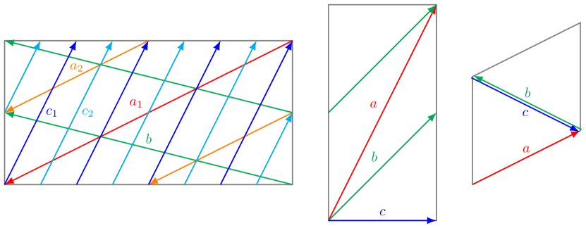
Refer to caption
Figure 13: Brane configuration for the three two-tori in Model 19-dual where the third two-torus is tilted. Fermion mass hierarchies result from the intersections on the first two-torus.
Table 14: The angles with respect to the orientifold plane made by the cycle wrapped by each stack of D-branes on each of the three two-tori in Model 19-dual.

19-dualθ1θ2θ3atan1(723)tan1(7232)tan1(4723)btan1(161)tan1(1612)0ctan1(4723)tan1(4723)tan1(4723)missing-subexpressionmissing-subexpressionmissing-subexpressionmissing-subexpression19-dualsuperscript𝜃1superscript𝜃2superscript𝜃3missing-subexpressionmissing-subexpressionmissing-subexpressionmissing-subexpression𝑎superscript1723superscript17232superscript14723missing-subexpressionmissing-subexpressionmissing-subexpressionmissing-subexpression𝑏superscript1161superscript116120missing-subexpressionmissing-subexpressionmissing-subexpressionmissing-subexpression𝑐superscript14723superscript14723superscript14723\begin{array}[]{|c|c|c|c|}\hline\cr\text{\hyperref@@ii[model19.5]{19-dual}}&\theta^{1}&\theta^{2}&\theta^{3}\\ \hline\cr a&\tan^{-1}\left(\sqrt{\frac{7}{23}}\right)&-\tan^{-1}\left(\frac{\sqrt{\frac{7}{23}}}{2}\right)&\tan^{-1}\left(4\sqrt{\frac{7}{23}}\right)\\ \hline\cr b&\tan^{-1}\left(\sqrt{161}\right)&\tan^{-1}\left(\frac{\sqrt{161}}{2}\right)&0\\ \hline\cr c&\tan^{-1}\left(4\sqrt{\frac{7}{23}}\right)&-\tan^{-1}\left(4\sqrt{\frac{7}{23}}\right)&-\tan^{-1}\left(4\sqrt{\frac{7}{23}}\right)\\ \hline\cr\end{array}

The complex structure moduli U𝑈U from (18) are,

{U1,U2,U3}subscript𝑈1subscript𝑈2subscript𝑈3\displaystyle\{U_{1},U_{2},U_{3}\} ={i723,i161,8135(28+i161)},absent𝑖723𝑖161813528𝑖161\displaystyle=\left\{i\sqrt{\frac{7}{23}},i\sqrt{161},\frac{8}{135}\left(28+i\sqrt{161}\right)\right\}, (220)

and the corresponding u𝑢u-moduli and s𝑠s-modulus in supergravity basis from (19) are,

{u1,u2,u3}subscript𝑢1subscript𝑢2subscript𝑢3\displaystyle\{u_{1},u_{2},u_{3}\} ={21614eϕ4π,274eϕ4233/4π,1614eϕ442π},absent24161superscript𝑒subscriptitalic-ϕ4𝜋247superscript𝑒subscriptitalic-ϕ4superscript2334𝜋4161superscript𝑒subscriptitalic-ϕ442𝜋\displaystyle=\left\{\frac{\sqrt{2}\sqrt[4]{161}e^{-\phi_{4}}}{\pi},\frac{\sqrt{2}\sqrt[4]{7}e^{-\phi_{4}}}{23^{3/4}\pi},\frac{\sqrt[4]{161}e^{-\phi_{4}}}{4\sqrt{2}\pi}\right\},
s𝑠\displaystyle s =234eϕ44273/4π.absent423superscript𝑒subscriptitalic-ϕ442superscript734𝜋\displaystyle=\frac{\sqrt[4]{23}e^{-\phi_{4}}}{4\sqrt{2}7^{3/4}\pi}. (221)

Using (24) and the values from the table A28, the gauge kinetic function becomes,

{fa,fb,fc}subscript𝑓𝑎subscript𝑓𝑏subscript𝑓𝑐\displaystyle\{f_{a},f_{b},f_{c}\} ={405eϕ4821613/4π,1485eϕ41621613/4π,135eϕ41621613/4π},absent405superscript𝑒subscriptitalic-ϕ482superscript16134𝜋1485superscript𝑒subscriptitalic-ϕ4162superscript16134𝜋135superscript𝑒subscriptitalic-ϕ4162superscript16134𝜋\displaystyle=\left\{\frac{405e^{-\phi_{4}}}{8\sqrt{2}161^{3/4}\pi},\frac{1485e^{-\phi_{4}}}{16\sqrt{2}161^{3/4}\pi},\frac{135e^{-\phi_{4}}}{16\sqrt{2}161^{3/4}\pi}\right\}, (222)

To calculate gaugino masses M1,2,3subscript𝑀123M_{1,2,3} respectively for U(1)YUsubscript1𝑌{\rm U}(1)_{Y}, SU(2)LSUsubscript2𝐿{\rm SU}(2)_{L} and SU(3)cSUsubscript3𝑐{\rm SU}(3)_{c} gauge groups, we first compute Ma,b,csubscript𝑀𝑎𝑏𝑐M_{a,b,c} using (3.2) as,

Masubscript𝑀𝑎\displaystyle M_{a} =m3/2(644Θ1+28Θ2+23(7Θ3+Θ4))2703,absentsubscript𝑚32644subscriptΘ128subscriptΘ2237subscriptΘ3subscriptΘ42703\displaystyle=\frac{m_{3/2}(644\Theta_{1}+28\Theta_{2}+23(7\Theta_{3}+\Theta_{4}))}{270\sqrt{3}},
Mbsubscript𝑀𝑏\displaystyle M_{b} =m3/2(1288Θ156Θ2+161Θ392Θ4)4953,absentsubscript𝑚321288subscriptΘ156subscriptΘ2161subscriptΘ392subscriptΘ44953\displaystyle=\frac{m_{3/2}(1288\Theta_{1}-56\Theta_{2}+161\Theta_{3}-92\Theta_{4})}{495\sqrt{3}},
Mcsubscript𝑀𝑐\displaystyle M_{c} =m3/2(112Θ223Θ4)453.absentsubscript𝑚32112subscriptΘ223subscriptΘ4453\displaystyle=\frac{m_{3/2}(112\Theta_{2}-23\Theta_{4})}{45\sqrt{3}}. (223)

Next, to compute the trilinear coupling and the sleptons mass-squared we require the angles, the differences of angles and their first and second order derivatives with respect to the moduli. In table 14 we show the angles (44) made by the cycle wrapped by each stack D6 branes with respect to the orientifold plane. The differences of the angles, θxyiθyiθxisuperscriptsubscript𝜃𝑥𝑦𝑖superscriptsubscript𝜃𝑦𝑖superscriptsubscript𝜃𝑥𝑖\theta_{xy}^{i}\equiv\theta_{y}^{i}-\theta_{x}^{i} are,

[{0.,0.,0.}{0.50991,0.0776874,0.850963}{0.217223,0.492148,0.70937}{0.50991,0.0776874,0.850963}{0.,0.,0.}{0.727132,0.41446,0.141593}{0.217223,0.492148,0.70937}{0.727132,0.41446,0.141593}{0.,0.,0.}]\displaystyle\hskip-10.00002pt\left[\begin{array}[]{ccc}\{0.,0.,0.\}&\{0.50991,-0.0776874,0.850963\}&\{-0.217223,-0.492148,0.70937\}\\ \{-0.50991,0.0776874,-0.850963\}&\{0.,0.,0.\}&\{-0.727132,-0.41446,-0.141593\}\\ \{0.217223,0.492148,-0.70937\}&\{0.727132,0.41446,0.141593\}&\{0.,0.,0.\}\\ \end{array}\right] (227)

To account for the negative angle differences it is convenient to define the sign function σxyisuperscriptsubscript𝜎𝑥𝑦𝑖\sigma_{xy}^{i}, which is 11-1 only for negative angle difference and +11+1 otherwise,

σxyi(1)1H(θxyi)superscriptsubscript𝜎𝑥𝑦𝑖superscript11𝐻superscriptsubscript𝜃𝑥𝑦𝑖\displaystyle\sigma_{xy}^{i}\equiv(-1)^{1-H(\theta_{xy}^{i})} =({1,1,1}{1,1,1}{1,1,1}{1,1,1}{1,1,1}{1,1,1}{1,1,1}{1,1,1}{1,1,1}),absent111111111111111111111111111\displaystyle=\left(\begin{array}[]{ccc}\{1,1,1\}&\{1,-1,1\}&\{-1,-1,1\}\\ \{-1,1,-1\}&\{1,1,1\}&\{-1,-1,-1\}\\ \{1,1,-1\}&\{1,1,1\}&\{1,1,1\}\\ \end{array}\right), (231)

where H(x)𝐻𝑥H(x) is the unit step function. And the function ηxysubscript𝜂𝑥𝑦\eta_{xy} can thus be defined by taking the product on the torus index i𝑖i as,

ηxyiσxyi=(111111111).subscript𝜂𝑥𝑦subscriptproduct𝑖superscriptsubscript𝜎𝑥𝑦𝑖111111111\eta_{xy}\equiv\prod_{i}\sigma_{xy}^{i}=\left(\begin{array}[]{ccc}1&-1&1\\ 1&1&-1\\ -1&1&1\\ \end{array}\right). (232)

Using the values of σxyisuperscriptsubscript𝜎𝑥𝑦𝑖\sigma_{xy}^{i} and ηxyisuperscriptsubscript𝜂𝑥𝑦𝑖\eta_{xy}^{i} in (60) we can compute the four cases of functions Ψ(θxy)Ψsubscript𝜃𝑥𝑦\Psi(\theta_{xy}) defined in (55) and (56). Similarly we calculate the derivative Ψ(θxyj)=dΨ(θxyj)dθxyjsuperscriptΨsubscriptsuperscript𝜃𝑗𝑥𝑦𝑑Ψsubscriptsuperscript𝜃𝑗𝑥𝑦𝑑subscriptsuperscript𝜃𝑗𝑥𝑦\Psi^{\prime}(\theta^{j}_{xy})=\frac{d\Psi(\theta^{j}_{xy})}{d\theta^{j}_{xy}} using equations (63), (3.3), (3.3) and the properties of digamma function ψ(0)(z)superscript𝜓0𝑧\psi^{(0)}(z) (3.3) while neglecting the contribution of the t𝑡t-moduli.

Utilizing above results while ignoring the CP-violating phases γisubscript𝛾𝑖\gamma_{i}, the the gaugino masses for the respective gauge groups U(1)YUsubscript1𝑌{\rm U}(1)_{Y}, SU(2)LSUsubscript2𝐿{\rm SU}(2)_{L} and SU(3)CSUsubscript3𝐶{\rm SU}(3)_{C}; the trilinear coupling (3.2); and squared-masses of squarks and sleptons (3.2) are obtained as follows,

MB~subscript𝑀~𝐵\displaystyle M_{\tilde{B}} MY=m3/2(1288Θ1+392Θ2+322Θ323Θ4)6753,absentsubscript𝑀𝑌subscript𝑚321288subscriptΘ1392subscriptΘ2322subscriptΘ323subscriptΘ46753\displaystyle\equiv M_{Y}=\frac{m_{3/2}(1288\Theta_{1}+392\Theta_{2}+322\Theta_{3}-23\Theta_{4})}{675\sqrt{3}},
MW~subscript𝑀~𝑊\displaystyle M_{\tilde{W}} Mb=m3/2(1288Θ156Θ2+161Θ392Θ4)4953,absentsubscript𝑀𝑏subscript𝑚321288subscriptΘ156subscriptΘ2161subscriptΘ392subscriptΘ44953\displaystyle\equiv M_{b}=\frac{m_{3/2}(1288\Theta_{1}-56\Theta_{2}+161\Theta_{3}-92\Theta_{4})}{495\sqrt{3}},
Mg~subscript𝑀~𝑔\displaystyle M_{\tilde{g}} Ma=m3/2(644Θ1+28Θ2+23(7Θ3+Θ4))2703,absentsubscript𝑀𝑎subscript𝑚32644subscriptΘ128subscriptΘ2237subscriptΘ3subscriptΘ42703\displaystyle\equiv M_{a}=\frac{m_{3/2}(644\Theta_{1}+28\Theta_{2}+23(7\Theta_{3}+\Theta_{4}))}{270\sqrt{3}},
A0subscript𝐴0\displaystyle A_{0} Aabc=m3/2(0.133497Θ11.55973Θ2+0.108067Θ30.146888Θ4),absentsubscript𝐴𝑎𝑏𝑐subscript𝑚320.133497subscriptΘ11.55973subscriptΘ20.108067subscriptΘ30.146888subscriptΘ4\displaystyle\equiv A_{abc}=m_{3/2}\Bigl{(}-0.133497\Theta_{1}-1.55973\Theta_{2}+0.108067\Theta_{3}-0.146888\Theta_{4}\Bigr{)},
mL2mab2subscriptsuperscript𝑚2𝐿subscriptsuperscript𝑚2𝑎𝑏\displaystyle m^{2}_{L}\equiv m^{2}_{ab} =m3/22(1.63243Θ1+21.90023Θ1Θ20.696574Θ1Θ3+1.49474Θ1Θ4\displaystyle=m_{3/2}^{2}\Bigl{(}-1.63243\Theta_{1}{}^{2}+1.90023\Theta_{1}\Theta_{2}-0.696574\Theta_{1}\Theta_{3}+1.49474\Theta_{1}\Theta_{4}
+0.770153Θ2+21.49862Θ2Θ31.898Θ2Θ41.96883Θ32\displaystyle\quad+0.770153\Theta_{2}{}^{2}+1.49862\Theta_{2}\Theta_{3}-1.898\Theta_{2}\Theta_{4}-1.96883\Theta_{3}{}^{2}
+1.08122Θ3Θ41.52482Θ4+21),\displaystyle\quad+1.08122\Theta_{3}\Theta_{4}-1.52482\Theta_{4}{}^{2}+1\Bigr{)},
mR2mac2subscriptsuperscript𝑚2𝑅subscriptsuperscript𝑚2𝑎𝑐\displaystyle m^{2}_{R}\equiv m^{2}_{ac} =m3/22(1.92219Θ120.606279Θ1Θ2+0.894634Θ1Θ30.207461Θ1Θ4\displaystyle=m_{3/2}^{2}\Bigl{(}-1.92219\Theta_{1}{}^{2}-0.606279\Theta_{1}\Theta_{2}+0.894634\Theta_{1}\Theta_{3}-0.207461\Theta_{1}\Theta_{4}
1.85446Θ2+20.894634Θ2Θ3+0.862019Θ2Θ40.50419Θ32\displaystyle\quad-1.85446\Theta_{2}{}^{2}+0.894634\Theta_{2}\Theta_{3}+0.862019\Theta_{2}\Theta_{4}-0.50419\Theta_{3}{}^{2}
+0.239164Θ3Θ40.506606Θ4+21).\displaystyle\quad+0.239164\Theta_{3}\Theta_{4}-0.506606\Theta_{4}{}^{2}+1\Bigr{)}. (233)

All soft terms are subject to the constraint (38).

4.13 Model 20

In Model 20 the three-point Yukawa couplings arise from the triplet intersections from the branes a𝑎a, b𝑏b and c𝑐c on the second two-torus with 9 pairs of Higgs from the 𝒩=2𝒩2\mathcal{N}=2 sector. Yukawa matrices for the Model 20 are of rank 3 and the three intersections required to form the disk diagrams for the Yukawa couplings all occur on the second torus as shown in figure 14.
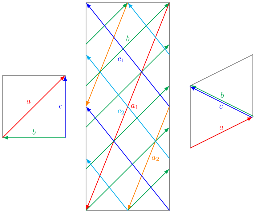
Refer to caption
Figure 14: Brane configuration for the three two-tori in Model 20 where the third two-torus is tilted. Fermion mass hierarchies result from the intersections on the second two-torus.
Table 15: The angles with respect to the orientifold plane made by the cycle wrapped by each stack of D-branes on each of the three two-tori in Model 20.

20θ1θ2θ3atan1(75)0π2btan1(5)tan1(25)tan1(52)ctan1(25)tan1(25)tan1(25)missing-subexpressionmissing-subexpressionmissing-subexpressionmissing-subexpression20superscript𝜃1superscript𝜃2superscript𝜃3missing-subexpressionmissing-subexpressionmissing-subexpressionmissing-subexpression𝑎superscript1750𝜋2missing-subexpressionmissing-subexpressionmissing-subexpressionmissing-subexpression𝑏superscript15superscript125superscript152missing-subexpressionmissing-subexpressionmissing-subexpressionmissing-subexpression𝑐superscript125superscript125superscript125\begin{array}[]{|c|c|c|c|}\hline\cr\text{\hyperref@@ii[model20]{20}}&\theta^{1}&\theta^{2}&\theta^{3}\\ \hline\cr a&\tan^{-1}\left(\frac{7}{\sqrt{5}}\right)&0&\frac{\pi}{2}\\ \hline\cr b&\tan^{-1}\left(\sqrt{5}\right)&\tan^{-1}\left(\frac{2}{\sqrt{5}}\right)&-\tan^{-1}\left(\frac{\sqrt{5}}{2}\right)\\ \hline\cr c&\tan^{-1}\left(\frac{2}{\sqrt{5}}\right)&-\tan^{-1}\left(\frac{2}{\sqrt{5}}\right)&-\tan^{-1}\left(\frac{2}{\sqrt{5}}\right)\\ \hline\cr\end{array}

The complex structure moduli U𝑈U from (18) are,

{U1,U2,U3}subscript𝑈1subscript𝑈2subscript𝑈3\displaystyle\{U_{1},U_{2},U_{3}\} ={7i5,i5,49(2+i5)},absent7𝑖5𝑖5492𝑖5\displaystyle=\left\{\frac{7i}{\sqrt{5}},i\sqrt{5},\frac{4}{9}\left(2+i\sqrt{5}\right)\right\}, (234)

and the corresponding u𝑢u-moduli and s𝑠s-modulus in supergravity basis from (19) are,

{u1,u2,u3}subscript𝑢1subscript𝑢2subscript𝑢3\displaystyle\{u_{1},u_{2},u_{3}\} ={54eϕ47π,7eϕ453/4π,547eϕ44π},absent45superscript𝑒subscriptitalic-ϕ47𝜋7superscript𝑒subscriptitalic-ϕ4superscript534𝜋457superscript𝑒subscriptitalic-ϕ44𝜋\displaystyle=\left\{\frac{\sqrt[4]{5}e^{-\phi_{4}}}{\sqrt{7}\pi},\frac{\sqrt{7}e^{-\phi_{4}}}{5^{3/4}\pi},\frac{\sqrt[4]{5}\sqrt{7}e^{-\phi_{4}}}{4\pi}\right\},
s𝑠\displaystyle s =54eϕ447π.absent45superscript𝑒subscriptitalic-ϕ447𝜋\displaystyle=\frac{\sqrt[4]{5}e^{-\phi_{4}}}{4\sqrt{7}\pi}. (235)

Using (24) and the values from the table A29, the gauge kinetic function becomes,

{fa,fb,fc}subscript𝑓𝑎subscript𝑓𝑏subscript𝑓𝑐\displaystyle\{f_{a},f_{b},f_{c}\} ={27eϕ48 53/47π,954eϕ4167π,97eϕ416 53/4π},absent27superscript𝑒subscriptitalic-ϕ4superscript85347𝜋945superscript𝑒subscriptitalic-ϕ4167𝜋97superscript𝑒subscriptitalic-ϕ4superscript16534𝜋\displaystyle=\left\{\frac{27e^{-\phi_{4}}}{8\ 5^{3/4}\sqrt{7}\pi},\frac{9\sqrt[4]{5}e^{-\phi_{4}}}{16\sqrt{7}\pi},\frac{9\sqrt{7}e^{-\phi_{4}}}{16\ 5^{3/4}\pi}\right\}, (236)

To calculate gaugino masses M1,2,3subscript𝑀123M_{1,2,3} respectively for U(1)YUsubscript1𝑌{\rm U}(1)_{Y}, SU(2)LSUsubscript2𝐿{\rm SU}(2)_{L} and SU(3)cSUsubscript3𝑐{\rm SU}(3)_{c} gauge groups, we first compute Ma,b,csubscript𝑀𝑎𝑏𝑐M_{a,b,c} using (3.2) as,

Masubscript𝑀𝑎\displaystyle M_{a} =m3/2(10Θ1+14Θ2+5(7Θ3+Θ4))183,absentsubscript𝑚3210subscriptΘ114subscriptΘ257subscriptΘ3subscriptΘ4183\displaystyle=\frac{m_{3/2}(10\Theta_{1}+14\Theta_{2}+5(7\Theta_{3}+\Theta_{4}))}{18\sqrt{3}},
Mbsubscript𝑀𝑏\displaystyle M_{b} =m3/2(4Θ15Θ4)33,absentsubscript𝑚324subscriptΘ15subscriptΘ433\displaystyle=\frac{m_{3/2}(4\Theta_{1}-5\Theta_{4})}{3\sqrt{3}},
Mcsubscript𝑀𝑐\displaystyle M_{c} =m3/2(4Θ2+5Θ3)33.absentsubscript𝑚324subscriptΘ25subscriptΘ333\displaystyle=\frac{m_{3/2}(4\Theta_{2}+5\Theta_{3})}{3\sqrt{3}}. (237)

Next, to compute the trilinear coupling and the sleptons mass-squared we require the angles, the differences of angles and their first and second order derivatives with respect to the moduli. In table 15 we show the angles (44) made by the cycle wrapped by each stack D6 branes with respect to the orientifold plane. The differences of the angles, θxyiθyiθxisuperscriptsubscript𝜃𝑥𝑦𝑖superscriptsubscript𝜃𝑦𝑖superscriptsubscript𝜃𝑥𝑖\theta_{xy}^{i}\equiv\theta_{y}^{i}-\theta_{x}^{i} are,

[{0.,0.,0.}{0.12001,0.721058,0.317863}{0.309193,0.291855,0.317863}{0.12001,0.721058,0.317863}{0.,0.,0.}{0.429204,0.429204,0.}{0.309193,0.291855,0.317863}{0.429204,0.429204,0.}{0.,0.,0.}]\displaystyle\hskip-10.00002pt\left[\begin{array}[]{ccc}\{0.,0.,0.\}&\{-0.12001,0.721058,-0.317863\}&\{0.309193,0.291855,-0.317863\}\\ \{0.12001,-0.721058,0.317863\}&\{0.,0.,0.\}&\{0.429204,-0.429204,0.\}\\ \{-0.309193,-0.291855,0.317863\}&\{-0.429204,0.429204,0.\}&\{0.,0.,0.\}\\ \end{array}\right] (241)

To account for the negative angle differences it is convenient to define the sign function σxyisuperscriptsubscript𝜎𝑥𝑦𝑖\sigma_{xy}^{i}, which is 11-1 only for negative angle difference and +11+1 otherwise,

σxyi(1)1H(θxyi)superscriptsubscript𝜎𝑥𝑦𝑖superscript11𝐻superscriptsubscript𝜃𝑥𝑦𝑖\displaystyle\sigma_{xy}^{i}\equiv(-1)^{1-H(\theta_{xy}^{i})} =({1,1,1}{1,1,1}{1,1,1}{1,1,1}{1,1,1}{1,1,1}{1,1,1}{1,1,1}{1,1,1}),absent111111111111111111111111111\displaystyle=\left(\begin{array}[]{ccc}\{1,1,1\}&\{-1,1,-1\}&\{1,1,-1\}\\ \{1,-1,1\}&\{1,1,1\}&\{1,-1,1\}\\ \{-1,-1,1\}&\{-1,1,1\}&\{1,1,1\}\\ \end{array}\right), (245)

where H(x)𝐻𝑥H(x) is the unit step function. And the function ηxysubscript𝜂𝑥𝑦\eta_{xy} can thus be defined by taking the product on the torus index i𝑖i as,

ηxyiσxyi=(111111111).subscript𝜂𝑥𝑦subscriptproduct𝑖superscriptsubscript𝜎𝑥𝑦𝑖111111111\eta_{xy}\equiv\prod_{i}\sigma_{xy}^{i}=\left(\begin{array}[]{ccc}1&1&-1\\ -1&1&-1\\ 1&-1&1\\ \end{array}\right). (246)

Using the values of σxyisuperscriptsubscript𝜎𝑥𝑦𝑖\sigma_{xy}^{i} and ηxyisuperscriptsubscript𝜂𝑥𝑦𝑖\eta_{xy}^{i} in (60) we can compute the four cases of functions Ψ(θxy)Ψsubscript𝜃𝑥𝑦\Psi(\theta_{xy}) defined in (55) and (56). Similarly we calculate the derivative Ψ(θxyj)=dΨ(θxyj)dθxyjsuperscriptΨsubscriptsuperscript𝜃𝑗𝑥𝑦𝑑Ψsubscriptsuperscript𝜃𝑗𝑥𝑦𝑑subscriptsuperscript𝜃𝑗𝑥𝑦\Psi^{\prime}(\theta^{j}_{xy})=\frac{d\Psi(\theta^{j}_{xy})}{d\theta^{j}_{xy}} using equations (63), (3.3), (3.3) and the properties of digamma function ψ(0)(z)superscript𝜓0𝑧\psi^{(0)}(z) (3.3) while neglecting the contribution of the t𝑡t-moduli.

Utilizing above results while ignoring the CP-violating phases γisubscript𝛾𝑖\gamma_{i}, the the gaugino masses for the respective gauge groups U(1)YUsubscript1𝑌{\rm U}(1)_{Y}, SU(2)LSUsubscript2𝐿{\rm SU}(2)_{L} and SU(3)CSUsubscript3𝐶{\rm SU}(3)_{C}; the trilinear coupling (3.2); and squared-masses of squarks and sleptons (3.2) are obtained as follows,

MB~subscript𝑀~𝐵\displaystyle M_{\tilde{B}} MY=m3/2(20Θ1+112Θ2+175Θ3+10Θ4)993,absentsubscript𝑀𝑌subscript𝑚3220subscriptΘ1112subscriptΘ2175subscriptΘ310subscriptΘ4993\displaystyle\equiv M_{Y}=\frac{m_{3/2}(20\Theta_{1}+112\Theta_{2}+175\Theta_{3}+10\Theta_{4})}{99\sqrt{3}},
MW~subscript𝑀~𝑊\displaystyle M_{\tilde{W}} Mb=m3/2(4Θ15Θ4)33,absentsubscript𝑀𝑏subscript𝑚324subscriptΘ15subscriptΘ433\displaystyle\equiv M_{b}=\frac{m_{3/2}(4\Theta_{1}-5\Theta_{4})}{3\sqrt{3}},
Mg~subscript𝑀~𝑔\displaystyle M_{\tilde{g}} Ma=m3/2(10Θ1+14Θ2+5(7Θ3+Θ4))183,absentsubscript𝑀𝑎subscript𝑚3210subscriptΘ114subscriptΘ257subscriptΘ3subscriptΘ4183\displaystyle\equiv M_{a}=\frac{m_{3/2}(10\Theta_{1}+14\Theta_{2}+5(7\Theta_{3}+\Theta_{4}))}{18\sqrt{3}},
A0subscript𝐴0\displaystyle A_{0} Aabc=m3/2(0.152188Θ11.57986Θ2+0.282383Θ30.282383Θ4),absentsubscript𝐴𝑎𝑏𝑐subscript𝑚320.152188subscriptΘ11.57986subscriptΘ20.282383subscriptΘ30.282383subscriptΘ4\displaystyle\equiv A_{abc}=m_{3/2}\Bigl{(}-0.152188\Theta_{1}-1.57986\Theta_{2}+0.282383\Theta_{3}-0.282383\Theta_{4}\Bigr{)},
mL2mab2subscriptsuperscript𝑚2𝐿subscriptsuperscript𝑚2𝑎𝑏\displaystyle m^{2}_{L}\equiv m^{2}_{ab} =m3/22(0.399003Θ1+21.25156Θ1Θ20.666067Θ1Θ30.958492Θ1Θ4\displaystyle=m_{3/2}^{2}\Bigl{(}-0.399003\Theta_{1}{}^{2}+1.25156\Theta_{1}\Theta_{2}-0.666067\Theta_{1}\Theta_{3}-0.958492\Theta_{1}\Theta_{4}
+0.106172Θ2+20.163812Θ2Θ30.73081Θ2Θ42.07593Θ32\displaystyle\quad+0.106172\Theta_{2}{}^{2}+0.163812\Theta_{2}\Theta_{3}-0.73081\Theta_{2}\Theta_{4}-2.07593\Theta_{3}{}^{2}
+1.71861Θ3Θ40.689841Θ4+21),\displaystyle\quad+1.71861\Theta_{3}\Theta_{4}-0.689841\Theta_{4}{}^{2}+1\Bigr{)},
mR2mac2subscriptsuperscript𝑚2𝑅subscriptsuperscript𝑚2𝑎𝑐\displaystyle m^{2}_{R}\equiv m^{2}_{ac} =m3/22(2.35521Θ121.21594Θ1Θ2+0.483768Θ1Θ3+1.51111Θ1Θ4\displaystyle=m_{3/2}^{2}\Bigl{(}-2.35521\Theta_{1}{}^{2}-1.21594\Theta_{1}\Theta_{2}+0.483768\Theta_{1}\Theta_{3}+1.51111\Theta_{1}\Theta_{4}
0.387583Θ2+21.12751Θ2Θ3+0.178197Θ2Θ4+0.0690201Θ32\displaystyle\quad-0.387583\Theta_{2}{}^{2}+1.12751\Theta_{2}\Theta_{3}+0.178197\Theta_{2}\Theta_{4}+0.0690201\Theta_{3}{}^{2}
1.68298Θ3Θ40.338871Θ4+21).\displaystyle\quad-1.68298\Theta_{3}\Theta_{4}-0.338871\Theta_{4}{}^{2}+1\Bigr{)}. (247)

All soft terms are subject to the constraint (38).

4.14 Model 20-dual

In Model 20-dual the three-point Yukawa couplings arise from the triplet intersections from the branes a𝑎a, b𝑏b and c𝑐c on the second two-torus with 9 pairs of Higgs from the 𝒩=2𝒩2\mathcal{N}=2 sector. Yukawa matrices for the Model 20-dual are of rank 3 and the three intersections required to form the disk diagrams for the Yukawa couplings all occur on the second torus as shown in figure 15.
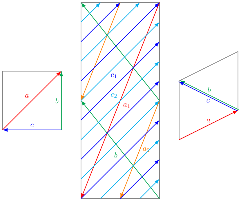
Refer to caption
Figure 15: Brane configuration for the three two-tori in Model 20-dual where the third two-torus is tilted. Fermion mass hierarchies result from the intersections on the second two-torus.
Table 16: The angles with respect to the orientifold plane made by the cycle wrapped by each stack of D-branes on each of the three two-tori in Model 20-dual.

20-dualθ1θ2θ3atan1(75)π20btan1(5)tan1(52)tan1(25)ctan1(25)tan1(25)tan1(25)missing-subexpressionmissing-subexpressionmissing-subexpressionmissing-subexpression20-dualsuperscript𝜃1superscript𝜃2superscript𝜃3missing-subexpressionmissing-subexpressionmissing-subexpressionmissing-subexpression𝑎superscript175𝜋20missing-subexpressionmissing-subexpressionmissing-subexpressionmissing-subexpression𝑏superscript15superscript152superscript125missing-subexpressionmissing-subexpressionmissing-subexpressionmissing-subexpression𝑐superscript125superscript125superscript125\begin{array}[]{|c|c|c|c|}\hline\cr\text{\hyperref@@ii[model20.5]{20-dual}}&\theta^{1}&\theta^{2}&\theta^{3}\\ \hline\cr a&\tan^{-1}\left(\frac{7}{\sqrt{5}}\right)&\frac{\pi}{2}&0\\ \hline\cr b&\tan^{-1}\left(\sqrt{5}\right)&-\tan^{-1}\left(\frac{\sqrt{5}}{2}\right)&\tan^{-1}\left(\frac{2}{\sqrt{5}}\right)\\ \hline\cr c&\tan^{-1}\left(\frac{2}{\sqrt{5}}\right)&-\tan^{-1}\left(\frac{2}{\sqrt{5}}\right)&-\tan^{-1}\left(\frac{2}{\sqrt{5}}\right)\\ \hline\cr\end{array}

The complex structure moduli U𝑈U from (18) are,

{U1,U2,U3}subscript𝑈1subscript𝑈2subscript𝑈3\displaystyle\{U_{1},U_{2},U_{3}\} ={7i5,i5,49(2+i5)},absent7𝑖5𝑖5492𝑖5\displaystyle=\left\{\frac{7i}{\sqrt{5}},i\sqrt{5},\frac{4}{9}\left(2+i\sqrt{5}\right)\right\}, (248)

and the corresponding u𝑢u-moduli and s𝑠s-modulus in supergravity basis from (19) are,

{u1,u2,u3}subscript𝑢1subscript𝑢2subscript𝑢3\displaystyle\{u_{1},u_{2},u_{3}\} ={54eϕ47π,7eϕ453/4π,547eϕ44π},absent45superscript𝑒subscriptitalic-ϕ47𝜋7superscript𝑒subscriptitalic-ϕ4superscript534𝜋457superscript𝑒subscriptitalic-ϕ44𝜋\displaystyle=\left\{\frac{\sqrt[4]{5}e^{-\phi_{4}}}{\sqrt{7}\pi},\frac{\sqrt{7}e^{-\phi_{4}}}{5^{3/4}\pi},\frac{\sqrt[4]{5}\sqrt{7}e^{-\phi_{4}}}{4\pi}\right\},
s𝑠\displaystyle s =54eϕ447π.absent45superscript𝑒subscriptitalic-ϕ447𝜋\displaystyle=\frac{\sqrt[4]{5}e^{-\phi_{4}}}{4\sqrt{7}\pi}. (249)

Using (24) and the values from the table A30, the gauge kinetic function becomes,

{fa,fb,fc}subscript𝑓𝑎subscript𝑓𝑏subscript𝑓𝑐\displaystyle\{f_{a},f_{b},f_{c}\} ={27eϕ48 53/47π,97eϕ416 53/4π,954eϕ4167π},absent27superscript𝑒subscriptitalic-ϕ4superscript85347𝜋97superscript𝑒subscriptitalic-ϕ4superscript16534𝜋945superscript𝑒subscriptitalic-ϕ4167𝜋\displaystyle=\left\{\frac{27e^{-\phi_{4}}}{8\ 5^{3/4}\sqrt{7}\pi},\frac{9\sqrt{7}e^{-\phi_{4}}}{16\ 5^{3/4}\pi},\frac{9\sqrt[4]{5}e^{-\phi_{4}}}{16\sqrt{7}\pi}\right\}, (250)

To calculate gaugino masses M1,2,3subscript𝑀123M_{1,2,3} respectively for U(1)YUsubscript1𝑌{\rm U}(1)_{Y}, SU(2)LSUsubscript2𝐿{\rm SU}(2)_{L} and SU(3)cSUsubscript3𝑐{\rm SU}(3)_{c} gauge groups, we first compute Ma,b,csubscript𝑀𝑎𝑏𝑐M_{a,b,c} using (3.2) as,

Masubscript𝑀𝑎\displaystyle M_{a} =m3/2(10Θ1+14Θ2+5(7Θ3+Θ4))183,absentsubscript𝑚3210subscriptΘ114subscriptΘ257subscriptΘ3subscriptΘ4183\displaystyle=\frac{m_{3/2}(10\Theta_{1}+14\Theta_{2}+5(7\Theta_{3}+\Theta_{4}))}{18\sqrt{3}},
Mbsubscript𝑀𝑏\displaystyle M_{b} =m3/2(4Θ2+5Θ3)33,absentsubscript𝑚324subscriptΘ25subscriptΘ333\displaystyle=\frac{m_{3/2}(4\Theta_{2}+5\Theta_{3})}{3\sqrt{3}},
Mcsubscript𝑀𝑐\displaystyle M_{c} =m3/2(4Θ15Θ4)33.absentsubscript𝑚324subscriptΘ15subscriptΘ433\displaystyle=\frac{m_{3/2}(4\Theta_{1}-5\Theta_{4})}{3\sqrt{3}}. (251)

Next, to compute the trilinear coupling and the sleptons mass-squared we require the angles, the differences of angles and their first and second order derivatives with respect to the moduli. In table 16 we show the angles (44) made by the cycle wrapped by each stack D6 branes with respect to the orientifold plane. The differences of the angles, θxyiθyiθxisuperscriptsubscript𝜃𝑥𝑦𝑖superscriptsubscript𝜃𝑦𝑖superscriptsubscript𝜃𝑥𝑖\theta_{xy}^{i}\equiv\theta_{y}^{i}-\theta_{x}^{i} are,

[{0.,0.,0.}{0.309193,0.291855,0.317863}{0.12001,0.721058,0.317863}{0.309193,0.291855,0.317863}{0.,0.,0.}{0.429204,0.429204,0.}{0.12001,0.721058,0.317863}{0.429204,0.429204,0.}{0.,0.,0.}]\displaystyle\hskip-10.00002pt\left[\begin{array}[]{ccc}\{0.,0.,0.\}&\{0.309193,0.291855,-0.317863\}&\{-0.12001,0.721058,-0.317863\}\\ \{-0.309193,-0.291855,0.317863\}&\{0.,0.,0.\}&\{-0.429204,0.429204,0.\}\\ \{0.12001,-0.721058,0.317863\}&\{0.429204,-0.429204,0.\}&\{0.,0.,0.\}\\ \end{array}\right] (255)

To account for the negative angle differences it is convenient to define the sign function σxyisuperscriptsubscript𝜎𝑥𝑦𝑖\sigma_{xy}^{i}, which is 11-1 only for negative angle difference and +11+1 otherwise,

σxyi(1)1H(θxyi)superscriptsubscript𝜎𝑥𝑦𝑖superscript11𝐻superscriptsubscript𝜃𝑥𝑦𝑖\displaystyle\sigma_{xy}^{i}\equiv(-1)^{1-H(\theta_{xy}^{i})} =({1,1,1}{1,1,1}{1,1,1}{1,1,1}{1,1,1}{1,1,1}{1,1,1}{1,1,1}{1,1,1}),absent111111111111111111111111111\displaystyle=\left(\begin{array}[]{ccc}\{1,1,1\}&\{1,1,-1\}&\{-1,1,-1\}\\ \{-1,-1,1\}&\{1,1,1\}&\{-1,1,1\}\\ \{1,-1,1\}&\{1,-1,1\}&\{1,1,1\}\\ \end{array}\right), (259)

where H(x)𝐻𝑥H(x) is the unit step function. And the function ηxysubscript𝜂𝑥𝑦\eta_{xy} can thus be defined by taking the product on the torus index i𝑖i as,

ηxyiσxyi=(111111111).subscript𝜂𝑥𝑦subscriptproduct𝑖superscriptsubscript𝜎𝑥𝑦𝑖111111111\eta_{xy}\equiv\prod_{i}\sigma_{xy}^{i}=\left(\begin{array}[]{ccc}1&-1&1\\ 1&1&-1\\ -1&-1&1\\ \end{array}\right). (260)

Using the values of σxyisuperscriptsubscript𝜎𝑥𝑦𝑖\sigma_{xy}^{i} and ηxyisuperscriptsubscript𝜂𝑥𝑦𝑖\eta_{xy}^{i} in (60) we can compute the four cases of functions Ψ(θxy)Ψsubscript𝜃𝑥𝑦\Psi(\theta_{xy}) defined in (55) and (56). Similarly we calculate the derivative Ψ(θxyj)=dΨ(θxyj)dθxyjsuperscriptΨsubscriptsuperscript𝜃𝑗𝑥𝑦𝑑Ψsubscriptsuperscript𝜃𝑗𝑥𝑦𝑑subscriptsuperscript𝜃𝑗𝑥𝑦\Psi^{\prime}(\theta^{j}_{xy})=\frac{d\Psi(\theta^{j}_{xy})}{d\theta^{j}_{xy}} using equations (63), (3.3), (3.3) and the properties of digamma function ψ(0)(z)superscript𝜓0𝑧\psi^{(0)}(z) (3.3) while neglecting the contribution of the t𝑡t-moduli.

Utilizing above results while ignoring the CP-violating phases γisubscript𝛾𝑖\gamma_{i}, the the gaugino masses for the respective gauge groups U(1)YUsubscript1𝑌{\rm U}(1)_{Y}, SU(2)LSUsubscript2𝐿{\rm SU}(2)_{L} and SU(3)CSUsubscript3𝐶{\rm SU}(3)_{C}; the trilinear coupling (3.2); and squared-masses of squarks and sleptons (3.2) are obtained as follows,

MB~subscript𝑀~𝐵\displaystyle M_{\tilde{B}} MY=m3/2(80Θ1+28Θ2+70Θ365Θ4)813,absentsubscript𝑀𝑌subscript𝑚3280subscriptΘ128subscriptΘ270subscriptΘ365subscriptΘ4813\displaystyle\equiv M_{Y}=\frac{m_{3/2}(80\Theta_{1}+28\Theta_{2}+70\Theta_{3}-65\Theta_{4})}{81\sqrt{3}},
MW~subscript𝑀~𝑊\displaystyle M_{\tilde{W}} Mb=m3/2(4Θ2+5Θ3)33,absentsubscript𝑀𝑏subscript𝑚324subscriptΘ25subscriptΘ333\displaystyle\equiv M_{b}=\frac{m_{3/2}(4\Theta_{2}+5\Theta_{3})}{3\sqrt{3}},
Mg~subscript𝑀~𝑔\displaystyle M_{\tilde{g}} Ma=m3/2(10Θ1+14Θ2+5(7Θ3+Θ4))183,absentsubscript𝑀𝑎subscript𝑚3210subscriptΘ114subscriptΘ257subscriptΘ3subscriptΘ4183\displaystyle\equiv M_{a}=\frac{m_{3/2}(10\Theta_{1}+14\Theta_{2}+5(7\Theta_{3}+\Theta_{4}))}{18\sqrt{3}},
A0subscript𝐴0\displaystyle A_{0} Aabc=m3/2(0.152188Θ11.57986Θ2+0.282383Θ30.282383Θ4),absentsubscript𝐴𝑎𝑏𝑐subscript𝑚320.152188subscriptΘ11.57986subscriptΘ20.282383subscriptΘ30.282383subscriptΘ4\displaystyle\equiv A_{abc}=m_{3/2}\Bigl{(}-0.152188\Theta_{1}-1.57986\Theta_{2}+0.282383\Theta_{3}-0.282383\Theta_{4}\Bigr{)},
mL2mab2subscriptsuperscript𝑚2𝐿subscriptsuperscript𝑚2𝑎𝑏\displaystyle m^{2}_{L}\equiv m^{2}_{ab} =m3/22(2.35521Θ121.21594Θ1Θ2+0.483768Θ1Θ3+1.51111Θ1Θ4\displaystyle=m_{3/2}^{2}\Bigl{(}-2.35521\Theta_{1}{}^{2}-1.21594\Theta_{1}\Theta_{2}+0.483768\Theta_{1}\Theta_{3}+1.51111\Theta_{1}\Theta_{4}
0.387583Θ2+21.12751Θ2Θ3+0.178197Θ2Θ4+0.0690201Θ32\displaystyle\quad-0.387583\Theta_{2}{}^{2}+1.12751\Theta_{2}\Theta_{3}+0.178197\Theta_{2}\Theta_{4}+0.0690201\Theta_{3}{}^{2}
1.68298Θ3Θ40.338871Θ4+21),\displaystyle\quad-1.68298\Theta_{3}\Theta_{4}-0.338871\Theta_{4}{}^{2}+1\Bigr{)},
mR2mac2subscriptsuperscript𝑚2𝑅subscriptsuperscript𝑚2𝑎𝑐\displaystyle m^{2}_{R}\equiv m^{2}_{ac} =m3/22(0.399003Θ1+21.25156Θ1Θ20.666067Θ1Θ30.958492Θ1Θ4\displaystyle=m_{3/2}^{2}\Bigl{(}-0.399003\Theta_{1}{}^{2}+1.25156\Theta_{1}\Theta_{2}-0.666067\Theta_{1}\Theta_{3}-0.958492\Theta_{1}\Theta_{4}
+0.106172Θ2+20.163812Θ2Θ30.73081Θ2Θ42.07593Θ32\displaystyle\quad+0.106172\Theta_{2}{}^{2}+0.163812\Theta_{2}\Theta_{3}-0.73081\Theta_{2}\Theta_{4}-2.07593\Theta_{3}{}^{2}
+1.71861Θ3Θ40.689841Θ4+21).\displaystyle\quad+1.71861\Theta_{3}\Theta_{4}-0.689841\Theta_{4}{}^{2}+1\Bigr{)}. (261)

All soft terms are subject to the constraint (38).

4.15 Model 21

In Model 21 the three-point Yukawa couplings arise from the triplet intersections from the branes a𝑎a, b𝑏b and c𝑐c on the second two-torus with 12 pairs of Higgs from the 𝒩=2𝒩2\mathcal{N}=2 sector. Yukawa matrices for the Model 21 are of rank 3 and the three intersections required to form the disk diagrams for the Yukawa couplings all occur on the second torus as shown in figure 16.
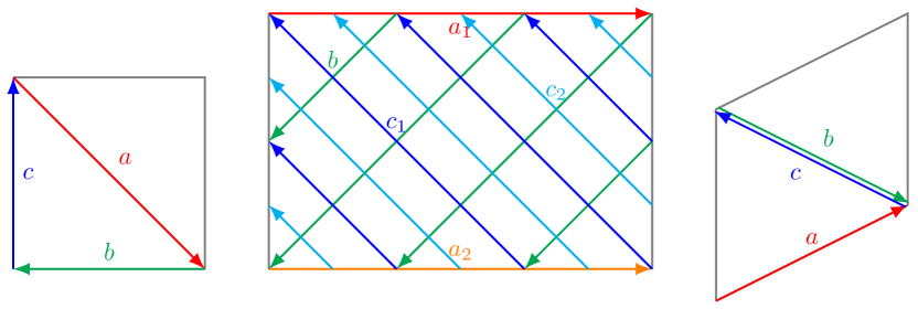
Refer to caption
Figure 16: Brane configuration for the three two-tori in Model 21 where the third two-torus is tilted. Fermion mass hierarchies result from the intersections on the second two-torus.
Table 17: The angles with respect to the orientifold plane made by the cycle wrapped by each stack of D-branes on each of the three two-tori in Model 21.

21θ1θ2θ3a3π40π2b0π43π4cπ43π43π4missing-subexpressionmissing-subexpressionmissing-subexpressionmissing-subexpression21superscript𝜃1superscript𝜃2superscript𝜃3missing-subexpressionmissing-subexpressionmissing-subexpressionmissing-subexpression𝑎3𝜋40𝜋2missing-subexpressionmissing-subexpressionmissing-subexpressionmissing-subexpression𝑏0𝜋43𝜋4missing-subexpressionmissing-subexpressionmissing-subexpressionmissing-subexpression𝑐𝜋43𝜋43𝜋4\begin{array}[]{|c|c|c|c|}\hline\cr\text{\hyperref@@ii[model21]{21}}&\theta^{1}&\theta^{2}&\theta^{3}\\ \hline\cr a&\frac{3\pi}{4}&0&\frac{\pi}{2}\\ \hline\cr b&0&\frac{\pi}{4}&\frac{3\pi}{4}\\ \hline\cr c&\frac{\pi}{4}&\frac{3\pi}{4}&\frac{3\pi}{4}\\ \hline\cr\end{array}

The complex structure moduli U𝑈U from (18) are,

{U1,U2,U3}subscript𝑈1subscript𝑈2subscript𝑈3\displaystyle\{U_{1},U_{2},U_{3}\} ={i,2i3,1+i},absent𝑖2𝑖31𝑖\displaystyle=\left\{i,\frac{2i}{3},1+i\right\}, (262)

and the corresponding u𝑢u-moduli and s𝑠s-modulus in supergravity basis from (19) are,

{u1,u2,u3}subscript𝑢1subscript𝑢2subscript𝑢3\displaystyle\{u_{1},u_{2},u_{3}\} ={eϕ43π,3eϕ42π,eϕ423π},absentsuperscript𝑒subscriptitalic-ϕ43𝜋3superscript𝑒subscriptitalic-ϕ42𝜋superscript𝑒subscriptitalic-ϕ423𝜋\displaystyle=\left\{\frac{e^{-\phi_{4}}}{\sqrt{3}\pi},\frac{\sqrt{3}e^{-\phi_{4}}}{2\pi},\frac{e^{-\phi_{4}}}{2\sqrt{3}\pi}\right\},
s𝑠\displaystyle s =3eϕ44π.absent3superscript𝑒subscriptitalic-ϕ44𝜋\displaystyle=\frac{\sqrt{3}e^{-\phi_{4}}}{4\pi}. (263)

Using (24) and the values from the table A31, the gauge kinetic function becomes,

{fa,fb,fc}subscript𝑓𝑎subscript𝑓𝑏subscript𝑓𝑐\displaystyle\{f_{a},f_{b},f_{c}\} ={3eϕ48π,3eϕ44π,3eϕ44π},absent3superscript𝑒subscriptitalic-ϕ48𝜋3superscript𝑒subscriptitalic-ϕ44𝜋3superscript𝑒subscriptitalic-ϕ44𝜋\displaystyle=\left\{\frac{\sqrt{3}e^{-\phi_{4}}}{8\pi},\frac{\sqrt{3}e^{-\phi_{4}}}{4\pi},\frac{\sqrt{3}e^{-\phi_{4}}}{4\pi}\right\}, (264)

To calculate gaugino masses M1,2,3subscript𝑀123M_{1,2,3} respectively for U(1)YUsubscript1𝑌{\rm U}(1)_{Y}, SU(2)LSUsubscript2𝐿{\rm SU}(2)_{L} and SU(3)cSUsubscript3𝑐{\rm SU}(3)_{c} gauge groups, we first compute Ma,b,csubscript𝑀𝑎𝑏𝑐M_{a,b,c} using (3.2) as,

Masubscript𝑀𝑎\displaystyle M_{a} =123m3/2(Θ2Θ4),absent123subscript𝑚32subscriptΘ2subscriptΘ4\displaystyle=\frac{1}{2}\sqrt{3}m_{3/2}(\Theta_{2}-\Theta_{4}),
Mbsubscript𝑀𝑏\displaystyle M_{b} =123m3/2(Θ1Θ4),absent123subscript𝑚32subscriptΘ1subscriptΘ4\displaystyle=\frac{1}{2}\sqrt{3}m_{3/2}(\Theta_{1}-\Theta_{4}),
Mcsubscript𝑀𝑐\displaystyle M_{c} =123m3/2(Θ2+Θ3).absent123subscript𝑚32subscriptΘ2subscriptΘ3\displaystyle=\frac{1}{2}\sqrt{3}m_{3/2}(\Theta_{2}+\Theta_{3}). (265)

Next, to compute the trilinear coupling and the sleptons mass-squared we require the angles, the differences of angles and their first and second order derivatives with respect to the moduli. In table 17 we show the angles (44) made by the cycle wrapped by each stack D6 branes with respect to the orientifold plane. The differences of the angles, θxyiθyiθxisuperscriptsubscript𝜃𝑥𝑦𝑖superscriptsubscript𝜃𝑦𝑖superscriptsubscript𝜃𝑥𝑖\theta_{xy}^{i}\equiv\theta_{y}^{i}-\theta_{x}^{i} are,

[{0.,0.,0.}{0.0730092,0.643806,0.570796}{0.356194,0.356194,0.429204}{0.0730092,0.643806,0.570796}{0.,0.,0.}{0.429204,0.287611,0.141593}{0.356194,0.356194,0.429204}{0.429204,0.287611,0.141593}{0.,0.,0.}]\displaystyle\hskip-10.00002pt\left[\begin{array}[]{ccc}\{0.,0.,0.\}&\{-0.0730092,0.643806,-0.570796\}&\{0.356194,0.356194,-0.429204\}\\ \{0.0730092,-0.643806,0.570796\}&\{0.,0.,0.\}&\{0.429204,-0.287611,0.141593\}\\ \{-0.356194,-0.356194,0.429204\}&\{-0.429204,0.287611,-0.141593\}&\{0.,0.,0.\}\\ \end{array}\right] (269)

To account for the negative angle differences it is convenient to define the sign function σxyisuperscriptsubscript𝜎𝑥𝑦𝑖\sigma_{xy}^{i}, which is 11-1 only for negative angle difference and +11+1 otherwise,

σxyi(1)1H(θxyi)superscriptsubscript𝜎𝑥𝑦𝑖superscript11𝐻superscriptsubscript𝜃𝑥𝑦𝑖\displaystyle\sigma_{xy}^{i}\equiv(-1)^{1-H(\theta_{xy}^{i})} =({1,1,1}{1,1,1}{1,1,1}{1,1,1}{1,1,1}{1,1,1}{1,1,1}{1,1,1}{1,1,1}),absent111111111111111111111111111\displaystyle=\left(\begin{array}[]{ccc}\{1,1,1\}&\{-1,1,-1\}&\{1,1,-1\}\\ \{1,-1,1\}&\{1,1,1\}&\{1,-1,1\}\\ \{-1,-1,1\}&\{-1,1,-1\}&\{1,1,1\}\\ \end{array}\right), (273)

where H(x)𝐻𝑥H(x) is the unit step function. And the function ηxysubscript𝜂𝑥𝑦\eta_{xy} can thus be defined by taking the product on the torus index i𝑖i as,

ηxyiσxyi=(111111111).subscript𝜂𝑥𝑦subscriptproduct𝑖superscriptsubscript𝜎𝑥𝑦𝑖111111111\eta_{xy}\equiv\prod_{i}\sigma_{xy}^{i}=\left(\begin{array}[]{ccc}1&1&-1\\ -1&1&-1\\ 1&1&1\\ \end{array}\right). (274)

Using the values of σxyisuperscriptsubscript𝜎𝑥𝑦𝑖\sigma_{xy}^{i} and ηxyisuperscriptsubscript𝜂𝑥𝑦𝑖\eta_{xy}^{i} in (60) we can compute the four cases of functions Ψ(θxy)Ψsubscript𝜃𝑥𝑦\Psi(\theta_{xy}) defined in (55) and (56). Similarly we calculate the derivative Ψ(θxyj)=dΨ(θxyj)dθxyjsuperscriptΨsubscriptsuperscript𝜃𝑗𝑥𝑦𝑑Ψsubscriptsuperscript𝜃𝑗𝑥𝑦𝑑subscriptsuperscript𝜃𝑗𝑥𝑦\Psi^{\prime}(\theta^{j}_{xy})=\frac{d\Psi(\theta^{j}_{xy})}{d\theta^{j}_{xy}} using equations (63), (3.3), (3.3) and the properties of digamma function ψ(0)(z)superscript𝜓0𝑧\psi^{(0)}(z) (3.3) while neglecting the contribution of the t𝑡t-moduli.

Utilizing above results while ignoring the CP-violating phases γisubscript𝛾𝑖\gamma_{i}, the the gaugino masses for the respective gauge groups U(1)YUsubscript1𝑌{\rm U}(1)_{Y}, SU(2)LSUsubscript2𝐿{\rm SU}(2)_{L} and SU(3)CSUsubscript3𝐶{\rm SU}(3)_{C}; the trilinear coupling (3.2); and squared-masses of squarks and sleptons (3.2) are obtained as follows,

MB~subscript𝑀~𝐵\displaystyle M_{\tilde{B}} MY=183m3/2(4Θ2+3Θ3Θ4),absentsubscript𝑀𝑌183subscript𝑚324subscriptΘ23subscriptΘ3subscriptΘ4\displaystyle\equiv M_{Y}=\frac{1}{8}\sqrt{3}m_{3/2}(4\Theta_{2}+3\Theta_{3}-\Theta_{4}),
MW~subscript𝑀~𝑊\displaystyle M_{\tilde{W}} Mb=123m3/2(Θ1Θ4),absentsubscript𝑀𝑏123subscript𝑚32subscriptΘ1subscriptΘ4\displaystyle\equiv M_{b}=\frac{1}{2}\sqrt{3}m_{3/2}(\Theta_{1}-\Theta_{4}),
Mg~subscript𝑀~𝑔\displaystyle M_{\tilde{g}} Ma=123m3/2(Θ2Θ4),absentsubscript𝑀𝑎123subscript𝑚32subscriptΘ2subscriptΘ4\displaystyle\equiv M_{a}=\frac{1}{2}\sqrt{3}m_{3/2}(\Theta_{2}-\Theta_{4}),
A0subscript𝐴0\displaystyle A_{0} Aabc=m3/2(0.444661Θ11.36219Θ2+0.260871Θ30.186075Θ4),absentsubscript𝐴𝑎𝑏𝑐subscript𝑚320.444661subscriptΘ11.36219subscriptΘ20.260871subscriptΘ30.186075subscriptΘ4\displaystyle\equiv A_{abc}=m_{3/2}\Bigl{(}-0.444661\Theta_{1}-1.36219\Theta_{2}+0.260871\Theta_{3}-0.186075\Theta_{4}\Bigr{)},
mL2mab2subscriptsuperscript𝑚2𝐿subscriptsuperscript𝑚2𝑎𝑏\displaystyle m^{2}_{L}\equiv m^{2}_{ab} =m3/22(0.0689562Θ1+21.52807Θ1Θ20.25782Θ1Θ30.582907Θ1Θ4\displaystyle=m_{3/2}^{2}\Bigl{(}-0.0689562\Theta_{1}{}^{2}+1.52807\Theta_{1}\Theta_{2}-0.25782\Theta_{1}\Theta_{3}-0.582907\Theta_{1}\Theta_{4}
0.127855Θ2+20.31395Θ2Θ30.623439Θ2Θ42.04994Θ32\displaystyle\quad-0.127855\Theta_{2}{}^{2}+0.31395\Theta_{2}\Theta_{3}-0.623439\Theta_{2}\Theta_{4}-2.04994\Theta_{3}{}^{2}
+1.23441Θ3Θ40.809377Θ4+21),\displaystyle\quad+1.23441\Theta_{3}\Theta_{4}-0.809377\Theta_{4}{}^{2}+1\Bigr{)},
mR2mac2subscriptsuperscript𝑚2𝑅subscriptsuperscript𝑚2𝑎𝑐\displaystyle m^{2}_{R}\equiv m^{2}_{ac} =m3/22(2.28519Θ121.00169Θ1Θ2+0.506454Θ1Θ3+1.26634Θ1Θ4\displaystyle=m_{3/2}^{2}\Bigl{(}-2.28519\Theta_{1}{}^{2}-1.00169\Theta_{1}\Theta_{2}+0.506454\Theta_{1}\Theta_{3}+1.26634\Theta_{1}\Theta_{4}
0.637087Θ2+21.13601Θ2Θ3+0.140834Θ2Θ40.0262168Θ32\displaystyle\quad-0.637087\Theta_{2}{}^{2}+1.13601\Theta_{2}\Theta_{3}+0.140834\Theta_{2}\Theta_{4}-0.0262168\Theta_{3}{}^{2}
1.1866Θ3Θ40.492648Θ4+21).\displaystyle\quad-1.1866\Theta_{3}\Theta_{4}-0.492648\Theta_{4}{}^{2}+1\Bigr{)}. (275)

All soft terms are subject to the constraint (38).

4.16 Model 22

In Model 22 the three-point Yukawa couplings arise from the triplet intersections from the branes a𝑎a, b𝑏b and c𝑐c on the first two-torus with 12 pairs of Higgs from the 𝒩=2𝒩2\mathcal{N}=2 sector. Yukawa matrices for the Model 22 are of rank 3 and the three intersections required to form the disk diagrams for the Yukawa couplings all occur on the first torus as shown in figure 17.

Refer to caption
Figure 17: Brane configuration for the three two-tori in Model 22 where the third two-torus is tilted. Fermion mass hierarchies result from the intersections on the first two-torus.
Table 18: The angles with respect to the orientifold plane made by the cycle wrapped by each stack of D-branes on each of the three two-tori in Model 22.

22θ1θ2θ3atan1(25)tan1(52)tan1(110)b0π2tan1(526)ctan1(25)tan1(25)tan1(25)missing-subexpressionmissing-subexpressionmissing-subexpressionmissing-subexpression22superscript𝜃1superscript𝜃2superscript𝜃3missing-subexpressionmissing-subexpressionmissing-subexpressionmissing-subexpression𝑎superscript125superscript152superscript1110missing-subexpressionmissing-subexpressionmissing-subexpressionmissing-subexpression𝑏0𝜋2superscript1526missing-subexpressionmissing-subexpressionmissing-subexpressionmissing-subexpression𝑐superscript125superscript125superscript125\begin{array}[]{|c|c|c|c|}\hline\cr\text{\hyperref@@ii[model22]{22}}&\theta^{1}&\theta^{2}&\theta^{3}\\ \hline\cr a&-\tan^{-1}\left(\sqrt{\frac{2}{5}}\right)&-\tan^{-1}\left(\sqrt{\frac{5}{2}}\right)&\tan^{-1}\left(\frac{1}{\sqrt{10}}\right)\\ \hline\cr b&0&\frac{\pi}{2}&\tan^{-1}\left(\frac{\sqrt{\frac{5}{2}}}{6}\right)\\ \hline\cr c&\tan^{-1}\left(\sqrt{\frac{2}{5}}\right)&-\tan^{-1}\left(\sqrt{\frac{2}{5}}\right)&-\tan^{-1}\left(\sqrt{\frac{2}{5}}\right)\\ \hline\cr\end{array}

The complex structure moduli U𝑈U from (18) are,

{U1,U2,U3}subscript𝑈1subscript𝑈2subscript𝑈3\displaystyle\{U_{1},U_{2},U_{3}\} ={i25,16i52,27(2+i10)},absent𝑖2516𝑖52272𝑖10\displaystyle=\left\{i\sqrt{\frac{2}{5}},\frac{1}{6}i\sqrt{\frac{5}{2}},\frac{2}{7}\left(2+i\sqrt{10}\right)\right\}, (276)

and the corresponding u𝑢u-moduli and s𝑠s-modulus in supergravity basis from (19) are,

{u1,u2,u3}subscript𝑢1subscript𝑢2subscript𝑢3\displaystyle\{u_{1},u_{2},u_{3}\} ={524eϕ423π,23/43eϕ453/4π,524eϕ443π},absent452superscript𝑒subscriptitalic-ϕ423𝜋superscript2343superscript𝑒subscriptitalic-ϕ4superscript534𝜋452superscript𝑒subscriptitalic-ϕ443𝜋\displaystyle=\left\{\frac{\sqrt[4]{\frac{5}{2}}e^{-\phi_{4}}}{2\sqrt{3}\pi},\frac{2^{3/4}\sqrt{3}e^{-\phi_{4}}}{5^{3/4}\pi},\frac{\sqrt[4]{\frac{5}{2}}e^{-\phi_{4}}}{4\sqrt{3}\pi}\right\},
s𝑠\displaystyle s =5243eϕ42π.absent4523superscript𝑒subscriptitalic-ϕ42𝜋\displaystyle=\frac{\sqrt[4]{\frac{5}{2}}\sqrt{3}e^{-\phi_{4}}}{2\pi}. (277)

Using (24) and the values from the table A32, the gauge kinetic function becomes,

{fa,fb,fc}subscript𝑓𝑎subscript𝑓𝑏subscript𝑓𝑐\displaystyle\{f_{a},f_{b},f_{c}\} ={73eϕ482453/4π,7524eϕ4163π,77eϕ41624353/4π},absent73superscript𝑒subscriptitalic-ϕ4842superscript534𝜋7452superscript𝑒subscriptitalic-ϕ4163𝜋77superscript𝑒subscriptitalic-ϕ416423superscript534𝜋\displaystyle=\left\{\frac{7\sqrt{3}e^{-\phi_{4}}}{8\sqrt[4]{2}5^{3/4}\pi},\frac{7\sqrt[4]{\frac{5}{2}}e^{-\phi_{4}}}{16\sqrt{3}\pi},\frac{77e^{-\phi_{4}}}{16\sqrt[4]{2}\sqrt{3}5^{3/4}\pi}\right\}, (278)

To calculate gaugino masses M1,2,3subscript𝑀123M_{1,2,3} respectively for U(1)YUsubscript1𝑌{\rm U}(1)_{Y}, SU(2)LSUsubscript2𝐿{\rm SU}(2)_{L} and SU(3)cSUsubscript3𝑐{\rm SU}(3)_{c} gauge groups, we first compute Ma,b,csubscript𝑀𝑎𝑏𝑐M_{a,b,c} using (3.2) as,

Masubscript𝑀𝑎\displaystyle M_{a} =173m3/2(2Θ25Θ4),absent173subscript𝑚322subscriptΘ25subscriptΘ4\displaystyle=\frac{1}{7}\sqrt{3}m_{3/2}(2\Theta_{2}-5\Theta_{4}),
Mbsubscript𝑀𝑏\displaystyle M_{b} =173m3/2(2Θ1+5Θ3),absent173subscript𝑚322subscriptΘ15subscriptΘ3\displaystyle=\frac{1}{7}\sqrt{3}m_{3/2}(2\Theta_{1}+5\Theta_{3}),
Mcsubscript𝑀𝑐\displaystyle M_{c} =1773m3/2(10Θ1+12Θ25(Θ3+12Θ4)).absent1773subscript𝑚3210subscriptΘ112subscriptΘ25subscriptΘ312subscriptΘ4\displaystyle=\frac{1}{77}\sqrt{3}m_{3/2}(10\Theta_{1}+12\Theta_{2}-5(\Theta_{3}+12\Theta_{4})). (279)

Next, to compute the trilinear coupling and the sleptons mass-squared we require the angles, the differences of angles and their first and second order derivatives with respect to the moduli. In table 18 we show the angles (44) made by the cycle wrapped by each stack D6 branes with respect to the orientifold plane. The differences of the angles, θxyiθyiθxisuperscriptsubscript𝜃𝑥𝑦𝑖superscriptsubscript𝜃𝑦𝑖superscriptsubscript𝜃𝑥𝑖\theta_{xy}^{i}\equiv\theta_{y}^{i}-\theta_{x}^{i} are,

[{0.,0.,0.}{0.301318,0.570796,0.0137074}{0.12978,0.257665,0.127885}{0.301318,0.570796,0.0137074}{0.,0.,0.}{0.171538,0.313131,0.141593}{0.12978,0.257665,0.127885}{0.171538,0.313131,0.141593}{0.,0.,0.}]\displaystyle\hskip-10.00002pt\left[\begin{array}[]{ccc}\{0.,0.,0.\}&\{-0.301318,0.570796,0.0137074\}&\{-0.12978,0.257665,-0.127885\}\\ \{0.301318,-0.570796,-0.0137074\}&\{0.,0.,0.\}&\{0.171538,-0.313131,-0.141593\}\\ \{0.12978,-0.257665,0.127885\}&\{-0.171538,0.313131,0.141593\}&\{0.,0.,0.\}\\ \end{array}\right] (283)

To account for the negative angle differences it is convenient to define the sign function σxyisuperscriptsubscript𝜎𝑥𝑦𝑖\sigma_{xy}^{i}, which is 11-1 only for negative angle difference and +11+1 otherwise,

σxyi(1)1H(θxyi)superscriptsubscript𝜎𝑥𝑦𝑖superscript11𝐻superscriptsubscript𝜃𝑥𝑦𝑖\displaystyle\sigma_{xy}^{i}\equiv(-1)^{1-H(\theta_{xy}^{i})} =({1,1,1}{1,1,1}{1,1,1}{1,1,1}{1,1,1}{1,1,1}{1,1,1}{1,1,1}{1,1,1}),absent111111111111111111111111111\displaystyle=\left(\begin{array}[]{ccc}\{1,1,1\}&\{-1,1,1\}&\{-1,1,-1\}\\ \{1,-1,-1\}&\{1,1,1\}&\{1,-1,-1\}\\ \{1,-1,1\}&\{-1,1,1\}&\{1,1,1\}\\ \end{array}\right), (287)

where H(x)𝐻𝑥H(x) is the unit step function. And the function ηxysubscript𝜂𝑥𝑦\eta_{xy} can thus be defined by taking the product on the torus index i𝑖i as,

ηxyiσxyi=(111111111).subscript𝜂𝑥𝑦subscriptproduct𝑖superscriptsubscript𝜎𝑥𝑦𝑖111111111\eta_{xy}\equiv\prod_{i}\sigma_{xy}^{i}=\left(\begin{array}[]{ccc}1&-1&1\\ 1&1&1\\ -1&-1&1\\ \end{array}\right). (288)

Using the values of σxyisuperscriptsubscript𝜎𝑥𝑦𝑖\sigma_{xy}^{i} and ηxyisuperscriptsubscript𝜂𝑥𝑦𝑖\eta_{xy}^{i} in (60) we can compute the four cases of functions Ψ(θxy)Ψsubscript𝜃𝑥𝑦\Psi(\theta_{xy}) defined in (55) and (56). Similarly we calculate the derivative Ψ(θxyj)=dΨ(θxyj)dθxyjsuperscriptΨsubscriptsuperscript𝜃𝑗𝑥𝑦𝑑Ψsubscriptsuperscript𝜃𝑗𝑥𝑦𝑑subscriptsuperscript𝜃𝑗𝑥𝑦\Psi^{\prime}(\theta^{j}_{xy})=\frac{d\Psi(\theta^{j}_{xy})}{d\theta^{j}_{xy}} using equations (63), (3.3), (3.3) and the properties of digamma function ψ(0)(z)superscript𝜓0𝑧\psi^{(0)}(z) (3.3) while neglecting the contribution of the t𝑡t-moduli.

Utilizing above results while ignoring the CP-violating phases γisubscript𝛾𝑖\gamma_{i}, the the gaugino masses for the respective gauge groups U(1)YUsubscript1𝑌{\rm U}(1)_{Y}, SU(2)LSUsubscript2𝐿{\rm SU}(2)_{L} and SU(3)CSUsubscript3𝐶{\rm SU}(3)_{C}; the trilinear coupling (3.2); and squared-masses of squarks and sleptons (3.2) are obtained as follows,

MB~subscript𝑀~𝐵\displaystyle M_{\tilde{B}} MY=m3/2(2Θ1+4Θ2Θ316Θ4)73,absentsubscript𝑀𝑌subscript𝑚322subscriptΘ14subscriptΘ2subscriptΘ316subscriptΘ473\displaystyle\equiv M_{Y}=\frac{m_{3/2}(2\Theta_{1}+4\Theta_{2}-\Theta_{3}-16\Theta_{4})}{7\sqrt{3}},
MW~subscript𝑀~𝑊\displaystyle M_{\tilde{W}} Mb=173m3/2(2Θ1+5Θ3),absentsubscript𝑀𝑏173subscript𝑚322subscriptΘ15subscriptΘ3\displaystyle\equiv M_{b}=\frac{1}{7}\sqrt{3}m_{3/2}(2\Theta_{1}+5\Theta_{3}),
Mg~subscript𝑀~𝑔\displaystyle M_{\tilde{g}} Ma=173m3/2(2Θ25Θ4),absentsubscript𝑀𝑎173subscript𝑚322subscriptΘ25subscriptΘ4\displaystyle\equiv M_{a}=\frac{1}{7}\sqrt{3}m_{3/2}(2\Theta_{2}-5\Theta_{4}),
A0subscript𝐴0\displaystyle A_{0} Aabc=m3/2(1.83963Θ11.52115Θ2+0.246437Θ3+1.38229Θ4),absentsubscript𝐴𝑎𝑏𝑐subscript𝑚321.83963subscriptΘ11.52115subscriptΘ20.246437subscriptΘ31.38229subscriptΘ4\displaystyle\equiv A_{abc}=m_{3/2}\Bigl{(}-1.83963\Theta_{1}-1.52115\Theta_{2}+0.246437\Theta_{3}+1.38229\Theta_{4}\Bigr{)},
mL2mab2subscriptsuperscript𝑚2𝐿subscriptsuperscript𝑚2𝑎𝑏\displaystyle m^{2}_{L}\equiv m^{2}_{ab} =m3/22(1.01495Θ120.356479Θ1Θ21.50575Θ1Θ30.924945Θ1Θ4\displaystyle=m_{3/2}^{2}\Bigl{(}1.01495\Theta_{1}{}^{2}-0.356479\Theta_{1}\Theta_{2}-1.50575\Theta_{1}\Theta_{3}-0.924945\Theta_{1}\Theta_{4}
+0.41741Θ221.65173Θ2Θ31.24068Θ2Θ40.642555Θ32\displaystyle\quad+0.41741\Theta_{2}{}^{2}-1.65173\Theta_{2}\Theta_{3}-1.24068\Theta_{2}\Theta_{4}-0.642555\Theta_{3}{}^{2}
+0.586882Θ3Θ40.632323Θ4+21),\displaystyle\quad+0.586882\Theta_{3}\Theta_{4}-0.632323\Theta_{4}{}^{2}+1\Bigr{)},
mR2mac2subscriptsuperscript𝑚2𝑅subscriptsuperscript𝑚2𝑎𝑐\displaystyle m^{2}_{R}\equiv m^{2}_{ac} =m3/22(0.668817Θ1+20.0838741Θ1Θ22.13002Θ1Θ30.767052Θ1Θ4\displaystyle=m_{3/2}^{2}\Bigl{(}0.668817\Theta_{1}{}^{2}+0.0838741\Theta_{1}\Theta_{2}-2.13002\Theta_{1}\Theta_{3}-0.767052\Theta_{1}\Theta_{4}
+0.714726Θ220.702234Θ2Θ32.08352Θ2Θ4+0.213147Θ32\displaystyle\quad+0.714726\Theta_{2}{}^{2}-0.702234\Theta_{2}\Theta_{3}-2.08352\Theta_{2}\Theta_{4}+0.213147\Theta_{3}{}^{2}
+1.43445Θ3Θ41.76444Θ4+21).\displaystyle\quad+1.43445\Theta_{3}\Theta_{4}-1.76444\Theta_{4}{}^{2}+1\Bigr{)}. (289)

All soft terms are subject to the constraint (38).

4.17 Model 22-dual

In Model 22-dual the three-point Yukawa couplings arise from the triplet intersections from the branes a𝑎a, b𝑏b and c𝑐c on the first two-torus with 12 pairs of Higgs from the 𝒩=2𝒩2\mathcal{N}=2 sector. Yukawa matrices for the Model 22-dual are of rank 3 and the three intersections required to form the disk diagrams for the Yukawa couplings all occur on the first torus as shown in figure 18.

Refer to caption
Figure 18: Brane configuration for the three two-tori in Model 22-dual where the third two-torus is tilted. Fermion mass hierarchies result from the intersections on the first two-torus.
Table 19: The angles with respect to the orientifold plane made by the cycle wrapped by each stack of D-branes on each of the three two-tori in Model 22-dual.

22-dualθ1θ2θ3atan1(25)tan1(110)tan1(52)b0tan1(526)π2ctan1(25)tan1(25)tan1(25)missing-subexpressionmissing-subexpressionmissing-subexpressionmissing-subexpression22-dualsuperscript𝜃1superscript𝜃2superscript𝜃3missing-subexpressionmissing-subexpressionmissing-subexpressionmissing-subexpression𝑎superscript125superscript1110superscript152missing-subexpressionmissing-subexpressionmissing-subexpressionmissing-subexpression𝑏0superscript1526𝜋2missing-subexpressionmissing-subexpressionmissing-subexpressionmissing-subexpression𝑐superscript125superscript125superscript125\begin{array}[]{|c|c|c|c|}\hline\cr\text{\hyperref@@ii[model22.5]{22-dual}}&\theta^{1}&\theta^{2}&\theta^{3}\\ \hline\cr a&-\tan^{-1}\left(\sqrt{\frac{2}{5}}\right)&\tan^{-1}\left(\frac{1}{\sqrt{10}}\right)&-\tan^{-1}\left(\sqrt{\frac{5}{2}}\right)\\ \hline\cr b&0&\tan^{-1}\left(\frac{\sqrt{\frac{5}{2}}}{6}\right)&\frac{\pi}{2}\\ \hline\cr c&\tan^{-1}\left(\sqrt{\frac{2}{5}}\right)&-\tan^{-1}\left(\sqrt{\frac{2}{5}}\right)&-\tan^{-1}\left(\sqrt{\frac{2}{5}}\right)\\ \hline\cr\end{array}

The complex structure moduli U𝑈U from (18) are,

{U1,U2,U3}subscript𝑈1subscript𝑈2subscript𝑈3\displaystyle\{U_{1},U_{2},U_{3}\} ={i25,16i52,27(2+i10)},absent𝑖2516𝑖52272𝑖10\displaystyle=\left\{i\sqrt{\frac{2}{5}},\frac{1}{6}i\sqrt{\frac{5}{2}},\frac{2}{7}\left(2+i\sqrt{10}\right)\right\}, (290)

and the corresponding u𝑢u-moduli and s𝑠s-modulus in supergravity basis from (19) are,

{u1,u2,u3}subscript𝑢1subscript𝑢2subscript𝑢3\displaystyle\{u_{1},u_{2},u_{3}\} ={524eϕ423π,23/43eϕ453/4π,524eϕ443π},absent452superscript𝑒subscriptitalic-ϕ423𝜋superscript2343superscript𝑒subscriptitalic-ϕ4superscript534𝜋452superscript𝑒subscriptitalic-ϕ443𝜋\displaystyle=\left\{\frac{\sqrt[4]{\frac{5}{2}}e^{-\phi_{4}}}{2\sqrt{3}\pi},\frac{2^{3/4}\sqrt{3}e^{-\phi_{4}}}{5^{3/4}\pi},\frac{\sqrt[4]{\frac{5}{2}}e^{-\phi_{4}}}{4\sqrt{3}\pi}\right\},
s𝑠\displaystyle s =5243eϕ42π.absent4523superscript𝑒subscriptitalic-ϕ42𝜋\displaystyle=\frac{\sqrt[4]{\frac{5}{2}}\sqrt{3}e^{-\phi_{4}}}{2\pi}. (291)

Using (24) and the values from the table A33, the gauge kinetic function becomes,

{fa,fb,fc}subscript𝑓𝑎subscript𝑓𝑏subscript𝑓𝑐\displaystyle\{f_{a},f_{b},f_{c}\} ={73eϕ482453/4π,77eϕ41624353/4π,7524eϕ4163π},absent73superscript𝑒subscriptitalic-ϕ4842superscript534𝜋77superscript𝑒subscriptitalic-ϕ416423superscript534𝜋7452superscript𝑒subscriptitalic-ϕ4163𝜋\displaystyle=\left\{\frac{7\sqrt{3}e^{-\phi_{4}}}{8\sqrt[4]{2}5^{3/4}\pi},\frac{77e^{-\phi_{4}}}{16\sqrt[4]{2}\sqrt{3}5^{3/4}\pi},\frac{7\sqrt[4]{\frac{5}{2}}e^{-\phi_{4}}}{16\sqrt{3}\pi}\right\}, (292)

To calculate gaugino masses M1,2,3subscript𝑀123M_{1,2,3} respectively for U(1)YUsubscript1𝑌{\rm U}(1)_{Y}, SU(2)LSUsubscript2𝐿{\rm SU}(2)_{L} and SU(3)cSUsubscript3𝑐{\rm SU}(3)_{c} gauge groups, we first compute Ma,b,csubscript𝑀𝑎𝑏𝑐M_{a,b,c} using (3.2) as,

Masubscript𝑀𝑎\displaystyle M_{a} =173m3/2(2Θ25Θ4),absent173subscript𝑚322subscriptΘ25subscriptΘ4\displaystyle=\frac{1}{7}\sqrt{3}m_{3/2}(2\Theta_{2}-5\Theta_{4}),
Mbsubscript𝑀𝑏\displaystyle M_{b} =1773m3/2(10Θ1+12Θ25(Θ3+12Θ4)),absent1773subscript𝑚3210subscriptΘ112subscriptΘ25subscriptΘ312subscriptΘ4\displaystyle=\frac{1}{77}\sqrt{3}m_{3/2}(10\Theta_{1}+12\Theta_{2}-5(\Theta_{3}+12\Theta_{4})),
Mcsubscript𝑀𝑐\displaystyle M_{c} =173m3/2(2Θ1+5Θ3).absent173subscript𝑚322subscriptΘ15subscriptΘ3\displaystyle=\frac{1}{7}\sqrt{3}m_{3/2}(2\Theta_{1}+5\Theta_{3}). (293)

Next, to compute the trilinear coupling and the sleptons mass-squared we require the angles, the differences of angles and their first and second order derivatives with respect to the moduli. In table 19 we show the angles (44) made by the cycle wrapped by each stack D6 branes with respect to the orientifold plane. The differences of the angles, θxyiθyiθxisuperscriptsubscript𝜃𝑥𝑦𝑖superscriptsubscript𝜃𝑦𝑖superscriptsubscript𝜃𝑥𝑖\theta_{xy}^{i}\equiv\theta_{y}^{i}-\theta_{x}^{i} are,

[{0.,0.,0.}{0.12978,0.257665,0.127885}{0.301318,0.570796,0.0137074}{0.12978,0.257665,0.127885}{0.,0.,0.}{0.171538,0.313131,0.141593}{0.301318,0.570796,0.0137074}{0.171538,0.313131,0.141593}{0.,0.,0.}]\displaystyle\hskip-10.00002pt\left[\begin{array}[]{ccc}\{0.,0.,0.\}&\{-0.12978,0.257665,-0.127885\}&\{-0.301318,0.570796,0.0137074\}\\ \{0.12978,-0.257665,0.127885\}&\{0.,0.,0.\}&\{-0.171538,0.313131,0.141593\}\\ \{0.301318,-0.570796,-0.0137074\}&\{0.171538,-0.313131,-0.141593\}&\{0.,0.,0.\}\\ \end{array}\right] (297)

To account for the negative angle differences it is convenient to define the sign function σxyisuperscriptsubscript𝜎𝑥𝑦𝑖\sigma_{xy}^{i}, which is 11-1 only for negative angle difference and +11+1 otherwise,

σxyi(1)1H(θxyi)superscriptsubscript𝜎𝑥𝑦𝑖superscript11𝐻superscriptsubscript𝜃𝑥𝑦𝑖\displaystyle\sigma_{xy}^{i}\equiv(-1)^{1-H(\theta_{xy}^{i})} =({1,1,1}{1,1,1}{1,1,1}{1,1,1}{1,1,1}{1,1,1}{1,1,1}{1,1,1}{1,1,1}),absent111111111111111111111111111\displaystyle=\left(\begin{array}[]{ccc}\{1,1,1\}&\{-1,1,-1\}&\{-1,1,1\}\\ \{1,-1,1\}&\{1,1,1\}&\{-1,1,1\}\\ \{1,-1,-1\}&\{1,-1,-1\}&\{1,1,1\}\\ \end{array}\right), (301)

where H(x)𝐻𝑥H(x) is the unit step function. And the function ηxysubscript𝜂𝑥𝑦\eta_{xy} can thus be defined by taking the product on the torus index i𝑖i as,

ηxyiσxyi=(111111111).subscript𝜂𝑥𝑦subscriptproduct𝑖superscriptsubscript𝜎𝑥𝑦𝑖111111111\eta_{xy}\equiv\prod_{i}\sigma_{xy}^{i}=\left(\begin{array}[]{ccc}1&1&-1\\ -1&1&-1\\ 1&1&1\\ \end{array}\right). (302)

Using the values of σxyisuperscriptsubscript𝜎𝑥𝑦𝑖\sigma_{xy}^{i} and ηxyisuperscriptsubscript𝜂𝑥𝑦𝑖\eta_{xy}^{i} in (60) we can compute the four cases of functions Ψ(θxy)Ψsubscript𝜃𝑥𝑦\Psi(\theta_{xy}) defined in (55) and (56). Similarly we calculate the derivative Ψ(θxyj)=dΨ(θxyj)dθxyjsuperscriptΨsubscriptsuperscript𝜃𝑗𝑥𝑦𝑑Ψsubscriptsuperscript𝜃𝑗𝑥𝑦𝑑subscriptsuperscript𝜃𝑗𝑥𝑦\Psi^{\prime}(\theta^{j}_{xy})=\frac{d\Psi(\theta^{j}_{xy})}{d\theta^{j}_{xy}} using equations (63), (3.3), (3.3) and the properties of digamma function ψ(0)(z)superscript𝜓0𝑧\psi^{(0)}(z) (3.3) while neglecting the contribution of the t𝑡t-moduli.

Utilizing above results while ignoring the CP-violating phases γisubscript𝛾𝑖\gamma_{i}, the the gaugino masses for the respective gauge groups U(1)YUsubscript1𝑌{\rm U}(1)_{Y}, SU(2)LSUsubscript2𝐿{\rm SU}(2)_{L} and SU(3)CSUsubscript3𝐶{\rm SU}(3)_{C}; the trilinear coupling (3.2); and squared-masses of squarks and sleptons (3.2) are obtained as follows,

MB~subscript𝑀~𝐵\displaystyle M_{\tilde{B}} MY=m3/2(10Θ1+8Θ2+25Θ320Θ4)213,absentsubscript𝑀𝑌subscript𝑚3210subscriptΘ18subscriptΘ225subscriptΘ320subscriptΘ4213\displaystyle\equiv M_{Y}=\frac{m_{3/2}(10\Theta_{1}+8\Theta_{2}+25\Theta_{3}-20\Theta_{4})}{21\sqrt{3}},
MW~subscript𝑀~𝑊\displaystyle M_{\tilde{W}} Mb=1773m3/2(10Θ1+12Θ25(Θ3+12Θ4)),absentsubscript𝑀𝑏1773subscript𝑚3210subscriptΘ112subscriptΘ25subscriptΘ312subscriptΘ4\displaystyle\equiv M_{b}=\frac{1}{77}\sqrt{3}m_{3/2}(10\Theta_{1}+12\Theta_{2}-5(\Theta_{3}+12\Theta_{4})),
Mg~subscript𝑀~𝑔\displaystyle M_{\tilde{g}} Ma=173m3/2(2Θ25Θ4),absentsubscript𝑀𝑎173subscript𝑚322subscriptΘ25subscriptΘ4\displaystyle\equiv M_{a}=\frac{1}{7}\sqrt{3}m_{3/2}(2\Theta_{2}-5\Theta_{4}),
A0subscript𝐴0\displaystyle A_{0} Aabc=m3/2(1.83963Θ11.52115Θ2+0.246437Θ3+1.38229Θ4),absentsubscript𝐴𝑎𝑏𝑐subscript𝑚321.83963subscriptΘ11.52115subscriptΘ20.246437subscriptΘ31.38229subscriptΘ4\displaystyle\equiv A_{abc}=m_{3/2}\Bigl{(}-1.83963\Theta_{1}-1.52115\Theta_{2}+0.246437\Theta_{3}+1.38229\Theta_{4}\Bigr{)},
mL2mab2subscriptsuperscript𝑚2𝐿subscriptsuperscript𝑚2𝑎𝑏\displaystyle m^{2}_{L}\equiv m^{2}_{ab} =m3/22(0.668817Θ1+20.0838741Θ1Θ22.13002Θ1Θ30.767052Θ1Θ4\displaystyle=m_{3/2}^{2}\Bigl{(}0.668817\Theta_{1}{}^{2}+0.0838741\Theta_{1}\Theta_{2}-2.13002\Theta_{1}\Theta_{3}-0.767052\Theta_{1}\Theta_{4}
+0.714726Θ220.702234Θ2Θ32.08352Θ2Θ4+0.213147Θ32\displaystyle\quad+0.714726\Theta_{2}{}^{2}-0.702234\Theta_{2}\Theta_{3}-2.08352\Theta_{2}\Theta_{4}+0.213147\Theta_{3}{}^{2}
+1.43445Θ3Θ41.76444Θ4+21),\displaystyle\quad+1.43445\Theta_{3}\Theta_{4}-1.76444\Theta_{4}{}^{2}+1\Bigr{)},
mR2mac2subscriptsuperscript𝑚2𝑅subscriptsuperscript𝑚2𝑎𝑐\displaystyle m^{2}_{R}\equiv m^{2}_{ac} =m3/22(1.01495Θ120.356479Θ1Θ21.50575Θ1Θ30.924945Θ1Θ4\displaystyle=m_{3/2}^{2}\Bigl{(}1.01495\Theta_{1}{}^{2}-0.356479\Theta_{1}\Theta_{2}-1.50575\Theta_{1}\Theta_{3}-0.924945\Theta_{1}\Theta_{4}
+0.41741Θ221.65173Θ2Θ31.24068Θ2Θ40.642555Θ32\displaystyle\quad+0.41741\Theta_{2}{}^{2}-1.65173\Theta_{2}\Theta_{3}-1.24068\Theta_{2}\Theta_{4}-0.642555\Theta_{3}{}^{2}
+0.586882Θ3Θ40.632323Θ4+21).\displaystyle\quad+0.586882\Theta_{3}\Theta_{4}-0.632323\Theta_{4}{}^{2}+1\Bigr{)}. (303)

All soft terms are subject to the constraint (38).

5 Discussion and conclusion

We have studied the supersymmetry breaking soft terms for all the viable models in the complete landscape of three-family supersymmetric Pati-Salam models arising from intersecting D6-branes on a 𝕋6/(2×2)superscript𝕋6subscript2subscript2\mathbbm{T}^{6}/(\mathbbm{Z}_{2}\times\mathbbm{Z}_{2}) orientifold in type IIA string theory, comprising 33 independent models with distinct string-scale gauge coupling relations. It is found that only 17 models contain viable Yukawa textures. We have focused on the u𝑢u-moduli dominated case together with the s𝑠s-moduli turned on, where the soft terms remain independent of the Yukawa couplings and the Wilson lines. The results for the trilinear coupling, gaugino-masses, squared-mass parameters of squarks, sleptons and Higgs depend on the brane wrapping numbers as well as supersymmetry breaking parameters which include the gravitino-mass parameter m3/2subscript𝑚32m_{3/2} and the goldstino angles ΘisubscriptΘ𝑖\Theta_{i}, i=1,2,3,4𝑖1234i=1,2,3,4.

In particular for the case of dual models under the exchange of two SU(2) sectors, the Yukawa couplings remain unchanged as discussed in Sabir:2024cgt , however, the corresponding soft term parameters only match for the trilinear coupling and the mass of the gluino. This can be explained by the internal geometry of the compact space where the Yukawa interactions depend only on the triangular area of the worldsheet instantons while the soft term parameters have an additional dependence on the orientation-angles of D6-branes in the three two-tori. Thus, the dual models besides having different gauge coupling relations also possess distinct masses of gauginos and squared-masses of squarks and sleptons. While it was already clear from the analysis of the Yukawa coupling Sabir:2024cgt that the best performing models in the entire landscape are the models 22 and 22-dual, the different result for susy breaking soft terms combined with experimental data for superpartners can in principle distinguish between the two models.

Our analysis reveals that the susy breaking soft terms are in general highly model dependent as evident from the results of section 4. Nonetheless, we have found a special limit under which the Higgs and the gaugino-masses in all of the models become degenerate. This limit corresponds to setting three goldstino angles to be equal to 1/2121/2 and taking dilaton angle to be 1/212-1/2, i.e. Θ1=Θ2=Θ3=Θs=1/2subscriptΘ1subscriptΘ2subscriptΘ3subscriptΘ𝑠12\Theta_{1}=\Theta_{2}=\Theta_{3}=-\Theta_{s}=1/2, provided that all CP-violating phases γisubscript𝛾𝑖\gamma_{i} are set to zero. Note that the special limit satisfies the crucial constraint (38) on the values of ΘisubscriptΘ𝑖\Theta_{i}. This results in following universal masses for the gauginos (viz. bino, wino and gluino) and the Higgs,

MB~=MW~=Mg~subscript𝑀~𝐵subscript𝑀~𝑊subscript𝑀~𝑔\displaystyle M_{\tilde{B}}=M_{\tilde{W}}=M_{\tilde{g}} =32m3/2m1/2,absent32subscript𝑚32subscript𝑚12\displaystyle=\frac{\sqrt{3}}{2}m_{3/2}\equiv m_{1/2},
mHsubscript𝑚𝐻\displaystyle m_{H} =12m3/2=13m1/2.absent12subscript𝑚3213subscript𝑚12\displaystyle=\frac{1}{2}m_{3/2}=\frac{1}{\sqrt{3}}m_{1/2}. (304)

Unlike the gaugino masses, the trilinear coupling A0subscript𝐴0A_{0} and the scalar squared-mass parameters of squarks and the sleptons, mL2subscriptsuperscript𝑚2𝐿m^{2}_{L} and mR2subscriptsuperscript𝑚2𝑅m^{2}_{R}, do not exhibit such universality and in general depend on the specific model parameters.

Given that the precise scale of supersymmetry remains uncertain, we defer further empirical investigations into supersymmetric partner spectra and the resultant neutralino relic density to future studies. It is noteworthy that string theory offers insights into the intricate phenomenology of superpartners through the wrapping numbers and the angles of intersecting D6-branes in the internal compact dimensions. However, additional experimental input is essential to fully leverage this mathematical framework.

Acknowledgements.
TL is supported in part by the National Key Research and Development Program of China Grant No. 2020YFC2201504, by the Projects No. 11875062, No. 11947302, No. 12047503, and No. 12275333 supported by the National Natural Science Foundation of China, by the Key Research Program of the Chinese Academy of Sciences, Grant No. XDPB15, by the Scientific Instrument Developing Project of the Chinese Academy of Sciences, Grant No. YJKYYQ20190049, and by the International Partnership Program of Chinese Academy of Sciences for Grand Challenges, Grant No. 112311KYSB20210012.

Appendix A Independent supersymmetric Pati-Salam models

We tabulate the 333333 independent models with distinct allowed gauge coupling relations in the three-family 𝒩=1𝒩1{\cal N}=1 supersymmetric Pati-Salam landscape arising from intersecting D6-branes on a type IIA 𝕋6/(2×2)superscript𝕋6subscript2subscript2\mathbbm{T}^{6}/(\mathbbm{Z}_{2}\times\mathbbm{Z}_{2}) orientifold He:2021gug ; Sabir:2024cgt .

Table A1: D6-brane configurations and intersection numbers of Model 1, and its MSSM gauge coupling relation is ga2=gb2=53gc2=25195gY23=423πeϕ4superscriptsubscript𝑔𝑎2superscriptsubscript𝑔𝑏253superscriptsubscript𝑔𝑐225195superscriptsubscript𝑔𝑌23423𝜋superscript𝑒subscriptitalic-ϕ4g_{a}^{2}=g_{b}^{2}=\frac{5}{3}g_{c}^{2}=\frac{25}{19}\frac{5g_{Y}^{2}}{3}=4\sqrt{\frac{2}{3}}\,\pi\,e^{\phi_{4}}.

Model 1U(4)C×U(2)L×U(2)R×USp(4)2×USp(4)4stackN(n1,l1)×(n2,l2)×(n3,l3)n\yng(2)n\yng(1,1)bbcc24a8(1,1)×(1,0)×(1,1)00303011b4(0,1)×(1,3)×(1,1)22--0410c4(2,1)×(1,1)×(1,1)26----12xA=13xB=xC=13xD24(1,0)×(0,1)×(0,2)β2g=2,β4g=2,χ1=1,χ2=13,χ3=244(0,1)×(0,1)×(2,0)missing-subexpressionmissing-subexpressionmissing-subexpressionmissing-subexpressionmissing-subexpressionmissing-subexpressionmissing-subexpressionmissing-subexpressionmissing-subexpressionmissing-subexpressionmissing-subexpressionModel 1Usubscript4𝐶Usubscript2𝐿Usubscript2𝑅USpsubscript42USpsubscript44missing-subexpressionmissing-subexpressionmissing-subexpressionmissing-subexpressionmissing-subexpressionmissing-subexpressionmissing-subexpressionmissing-subexpressionmissing-subexpressionmissing-subexpressionmissing-subexpressionmissing-subexpressionmissing-subexpressionmissing-subexpressionmissing-subexpressionmissing-subexpressionmissing-subexpressionmissing-subexpressionmissing-subexpressionmissing-subexpressionmissing-subexpressionmissing-subexpressionstack𝑁superscript𝑛1superscript𝑙1superscript𝑛2superscript𝑙2superscript𝑛3superscript𝑙3subscript𝑛\yng2subscript𝑛\yng11𝑏superscript𝑏𝑐superscript𝑐24missing-subexpressionmissing-subexpressionmissing-subexpressionmissing-subexpressionmissing-subexpressionmissing-subexpressionmissing-subexpressionmissing-subexpressionmissing-subexpressionmissing-subexpressionmissing-subexpression𝑎811101100303011𝑏401131122--0410𝑐421111126----12missing-subexpressionmissing-subexpressionmissing-subexpressionmissing-subexpressionmissing-subexpressionmissing-subexpressionmissing-subexpressionmissing-subexpressionmissing-subexpressionmissing-subexpressionmissing-subexpressionmissing-subexpressionmissing-subexpressionmissing-subexpressionsubscript𝑥𝐴13subscript𝑥𝐵subscript𝑥𝐶13subscript𝑥𝐷24100102formulae-sequencesubscriptsuperscript𝛽𝑔22subscriptsuperscript𝛽𝑔42missing-subexpressionmissing-subexpressionmissing-subexpressionformulae-sequencesubscript𝜒11formulae-sequencesubscript𝜒213subscript𝜒3244010120missing-subexpression\begin{array}[]{|c|c|c|c|c|c|c|c|c|c|c|}\hline\cr\vrule\lx@intercol\hfil\text{Model~{}\hyperref@@ii[spec1]{1}}\hfil\lx@intercol\vrule\lx@intercol&\lx@intercol\hfil{\textrm{U}(4)_{C}\times\textrm{U}(2)_{L}\times\textrm{U}(2)_{R}\times\textrm{USp}(4)_{2}\times\textrm{USp}(4)_{4}}\hfil\lx@intercol\vrule\lx@intercol\\ \hline\cr\hline\cr\rm{stack}&N&(n^{1},l^{1})\times(n^{2},l^{2})\times(n^{3},l^{3})&n_{\yng(2)}&n_{\yng(1,1)}&b&b^{\prime}&c&c^{\prime}&2&4\\ \hline\cr a&8&(1,-1)\times(1,0)\times(1,1)&0&0&3&0&-3&0&-1&1\\ b&4&(0,1)\times(-1,3)\times(-1,1)&2&-2&\text{-}&\text{-}&0&-4&1&0\\ c&4&(-2,-1)\times(-1,-1)\times(1,-1)&2&6&\text{-}&\text{-}&\text{-}&\text{-}&1&-2\\ \hline\cr&&&\lx@intercol\hfil x_{A}=\frac{1}{3}x_{B}=x_{C}=\frac{1}{3}x_{D}\hfil\lx@intercol\vrule\lx@intercol\\ 2&4&(1,0)\times(0,-1)\times(0,2)&\lx@intercol\hfil~{}\beta^{g}_{2}=-2,~{}\beta^{g}_{4}=-2,\hfil\lx@intercol\vrule\lx@intercol\\ &&&\lx@intercol\hfil\chi_{1}=1,~{}\chi_{2}=\frac{1}{3},~{}\chi_{3}=2\hfil\lx@intercol\vrule\lx@intercol\\ 4&4&(0,-1)\times(0,1)\times(2,0)&\lx@intercol\hfil\hfil\lx@intercol\vrule\lx@intercol\\ \hline\cr\end{array}

Table A2: D6-brane configurations and intersection numbers of Model 1-dual, and its MSSM gauge coupling relation is ga2=53gb2=gc2=5gY23=423πeϕ4superscriptsubscript𝑔𝑎253superscriptsubscript𝑔𝑏2superscriptsubscript𝑔𝑐25superscriptsubscript𝑔𝑌23423𝜋superscript𝑒subscriptitalic-ϕ4g_{a}^{2}=\frac{5}{3}g_{b}^{2}=g_{c}^{2}=\frac{5g_{Y}^{2}}{3}=4\sqrt{\frac{2}{3}}\,\pi\,e^{\phi_{4}}.

Model 1-dualU(4)C×U(2)L×U(2)R×USp(4)2×USp(4)4stackN(n1,l1)×(n2,l2)×(n3,l3)n\yng(2)n\yng(1,1)bbcc24a8(1,1)×(1,0)×(1,1)00303011b4(2,1)×(1,1)×(1,1)26--0412c4(0,1)×(1,3)×(1,1)22----10xA=13xB=xC=13xD24(1,0)×(0,1)×(0,2)β2g=2,β4g=2,χ1=1,χ2=13,χ3=244(0,1)×(0,1)×(2,0)missing-subexpressionmissing-subexpressionmissing-subexpressionmissing-subexpressionmissing-subexpressionmissing-subexpressionmissing-subexpressionmissing-subexpressionmissing-subexpressionmissing-subexpressionmissing-subexpressionModel 1-dualUsubscript4𝐶Usubscript2𝐿Usubscript2𝑅USpsubscript42USpsubscript44missing-subexpressionmissing-subexpressionmissing-subexpressionmissing-subexpressionmissing-subexpressionmissing-subexpressionmissing-subexpressionmissing-subexpressionmissing-subexpressionmissing-subexpressionmissing-subexpressionmissing-subexpressionmissing-subexpressionmissing-subexpressionmissing-subexpressionmissing-subexpressionmissing-subexpressionmissing-subexpressionmissing-subexpressionmissing-subexpressionmissing-subexpressionmissing-subexpressionstack𝑁superscript𝑛1superscript𝑙1superscript𝑛2superscript𝑙2superscript𝑛3superscript𝑙3subscript𝑛\yng2subscript𝑛\yng11𝑏superscript𝑏𝑐superscript𝑐24missing-subexpressionmissing-subexpressionmissing-subexpressionmissing-subexpressionmissing-subexpressionmissing-subexpressionmissing-subexpressionmissing-subexpressionmissing-subexpressionmissing-subexpressionmissing-subexpression𝑎811101100303011𝑏421111126--0412𝑐401131122----10missing-subexpressionmissing-subexpressionmissing-subexpressionmissing-subexpressionmissing-subexpressionmissing-subexpressionmissing-subexpressionmissing-subexpressionmissing-subexpressionmissing-subexpressionmissing-subexpressionmissing-subexpressionmissing-subexpressionmissing-subexpressionsubscript𝑥𝐴13subscript𝑥𝐵subscript𝑥𝐶13subscript𝑥𝐷24100102formulae-sequencesubscriptsuperscript𝛽𝑔22subscriptsuperscript𝛽𝑔42missing-subexpressionmissing-subexpressionmissing-subexpressionformulae-sequencesubscript𝜒11formulae-sequencesubscript𝜒213subscript𝜒3244010120missing-subexpression\begin{array}[]{|c|c|c|c|c|c|c|c|c|c|c|}\hline\cr\vrule\lx@intercol\hfil\text{Model~{}\hyperref@@ii[spec1.5]{1-dual}}\hfil\lx@intercol\vrule\lx@intercol&\lx@intercol\hfil{\textrm{U}(4)_{C}\times\textrm{U}(2)_{L}\times\textrm{U}(2)_{R}\times\textrm{USp}(4)_{2}\times\textrm{USp}(4)_{4}}\hfil\lx@intercol\vrule\lx@intercol\\ \hline\cr\hline\cr\rm{stack}&N&(n^{1},l^{1})\times(n^{2},l^{2})\times(n^{3},l^{3})&n_{\yng(2)}&n_{\yng(1,1)}&b&b^{\prime}&c&c^{\prime}&2&4\\ \hline\cr a&8&(1,-1)\times(1,0)\times(1,1)&0&0&-3&0&3&0&-1&1\\ b&4&(-2,-1)\times(-1,-1)\times(1,-1)&2&6&\text{-}&\text{-}&0&-4&1&-2\\ c&4&(0,1)\times(-1,3)\times(-1,1)&2&-2&\text{-}&\text{-}&\text{-}&\text{-}&1&0\\ \hline\cr&&&\lx@intercol\hfil x_{A}=\frac{1}{3}x_{B}=x_{C}=\frac{1}{3}x_{D}\hfil\lx@intercol\vrule\lx@intercol\\ 2&4&(1,0)\times(0,-1)\times(0,2)&\lx@intercol\hfil~{}\beta^{g}_{2}=-2,~{}\beta^{g}_{4}=-2,\hfil\lx@intercol\vrule\lx@intercol\\ &&&\lx@intercol\hfil\chi_{1}=1,~{}\chi_{2}=\frac{1}{3},~{}\chi_{3}=2\hfil\lx@intercol\vrule\lx@intercol\\ 4&4&(0,-1)\times(0,1)\times(2,0)&\lx@intercol\hfil\hfil\lx@intercol\vrule\lx@intercol\\ \hline\cr\end{array}

Table A3: D6-brane configurations and intersection numbers of Model 2, and its MSSM gauge coupling relation is ga2=95gb2=gc2=5gY23=1252πeϕ4superscriptsubscript𝑔𝑎295superscriptsubscript𝑔𝑏2superscriptsubscript𝑔𝑐25superscriptsubscript𝑔𝑌231252𝜋superscript𝑒subscriptitalic-ϕ4g_{a}^{2}=\frac{9}{5}g_{b}^{2}=g_{c}^{2}=\frac{5g_{Y}^{2}}{3}=\frac{12}{5}\sqrt{2}\,\pi\,e^{\phi_{4}}.

Model 2U(4)C×U(2)L×U(2)R×USp(2)1×USp(2)2×USp(2)3×USp(2)4stackN(n1,l1)×(n2,l2)×(n3,l3)n\yng(2)n\yng(1,1)bbcc1234a8(1,1)×(1,0)×(1,1)0021300101b4(1,0)×(1,1)×(1,3)22--440013c4(0,1)×(1,3)×(1,1)22----310012(1,0)×(1,0)×(2,0)xA=13xB=19xC=13xD22(1,0)×(0,1)×(0,2)β1g=3,β2g=3,β3g=5,β4g=1,32(0,1)×(1,0)×(0,2)χ1=13,χ2=1,χ3=2342(0,1)×(0,1)×(2,0)missing-subexpressionmissing-subexpressionmissing-subexpressionmissing-subexpressionmissing-subexpressionmissing-subexpressionmissing-subexpressionmissing-subexpressionmissing-subexpressionmissing-subexpressionmissing-subexpressionmissing-subexpressionmissing-subexpressionModel 2Usubscript4𝐶Usubscript2𝐿Usubscript2𝑅USpsubscript21USpsubscript22USpsubscript23USpsubscript24missing-subexpressionmissing-subexpressionmissing-subexpressionmissing-subexpressionmissing-subexpressionmissing-subexpressionmissing-subexpressionmissing-subexpressionmissing-subexpressionmissing-subexpressionmissing-subexpressionmissing-subexpressionmissing-subexpressionmissing-subexpressionmissing-subexpressionmissing-subexpressionmissing-subexpressionmissing-subexpressionmissing-subexpressionmissing-subexpressionmissing-subexpressionmissing-subexpressionmissing-subexpressionmissing-subexpressionmissing-subexpressionmissing-subexpressionstack𝑁superscript𝑛1superscript𝑙1superscript𝑛2superscript𝑙2superscript𝑛3superscript𝑙3subscript𝑛\yng2subscript𝑛\yng11𝑏superscript𝑏𝑐superscript𝑐1234missing-subexpressionmissing-subexpressionmissing-subexpressionmissing-subexpressionmissing-subexpressionmissing-subexpressionmissing-subexpressionmissing-subexpressionmissing-subexpressionmissing-subexpressionmissing-subexpressionmissing-subexpressionmissing-subexpression𝑎81110110021300101𝑏410111322--440013𝑐401131122----3100missing-subexpressionmissing-subexpressionmissing-subexpressionmissing-subexpressionmissing-subexpressionmissing-subexpressionmissing-subexpressionmissing-subexpressionmissing-subexpressionmissing-subexpressionmissing-subexpressionmissing-subexpressionmissing-subexpression12101020subscript𝑥𝐴13subscript𝑥𝐵19subscript𝑥𝐶13subscript𝑥𝐷22100102formulae-sequencesubscriptsuperscript𝛽𝑔13formulae-sequencesubscriptsuperscript𝛽𝑔23formulae-sequencesubscriptsuperscript𝛽𝑔35subscriptsuperscript𝛽𝑔4132011002formulae-sequencesubscript𝜒113formulae-sequencesubscript𝜒21subscript𝜒32342010120missing-subexpression\begin{array}[]{|c|c|c|c|c|c|c|c|c|c|c|c|c|}\hline\cr\vrule\lx@intercol\hfil\text{Model~{}\hyperref@@ii[spec2]{2}}\hfil\lx@intercol\vrule\lx@intercol&\lx@intercol\hfil{\textrm{U}(4)_{C}\times\textrm{U}(2)_{L}\times\textrm{U}(2)_{R}\times\textrm{USp}(2)_{1}\times\textrm{USp}(2)_{2}\times\textrm{USp}(2)_{3}\times\textrm{USp}(2)_{4}}\hfil\lx@intercol\vrule\lx@intercol\\ \hline\cr\hline\cr\rm{stack}&N&(n^{1},l^{1})\times(n^{2},l^{2})\times(n^{3},l^{3})&n_{\yng(2)}&n_{\yng(1,1)}&b&b^{\prime}&c&c^{\prime}&1&2&3&4\\ \hline\cr a&8&(1,-1)\times(1,0)\times(1,1)&0&0&-2&-1&3&0&0&-1&0&1\\ b&4&(-1,0)\times(-1,-1)\times(1,-3)&2&-2&\text{-}&\text{-}&-4&-4&0&0&1&-3\\ c&4&(0,1)\times(-1,3)\times(-1,1)&2&-2&\text{-}&\text{-}&\text{-}&\text{-}&-3&1&0&0\\ \hline\cr 1&2&(1,0)\times(1,0)\times(2,0)&\lx@intercol\hfil x_{A}=\frac{1}{3}x_{B}=\frac{1}{9}x_{C}=\frac{1}{3}x_{D}\hfil\lx@intercol\vrule\lx@intercol\\ 2&2&(1,0)\times(0,-1)\times(0,2)&\lx@intercol\hfil\beta^{g}_{1}=-3,~{}\beta^{g}_{2}=-3,~{}\beta^{g}_{3}=-5,~{}\beta^{g}_{4}=-1,\hfil\lx@intercol\vrule\lx@intercol\\ 3&2&(0,-1)\times(1,0)\times(0,2)&\lx@intercol\hfil\chi_{1}=\frac{1}{3},~{}\chi_{2}=1,~{}\chi_{3}=\frac{2}{3}\hfil\lx@intercol\vrule\lx@intercol\\ 4&2&(0,-1)\times(0,1)\times(2,0)&\lx@intercol\hfil\hfil\lx@intercol\vrule\lx@intercol\\ \hline\cr\end{array}

Table A4: D6-brane configurations and intersection numbers of Model 3, and its MSSM gauge coupling relation is ga2=12gb2=136gc2=65445gY23=16523πeϕ4superscriptsubscript𝑔𝑎212superscriptsubscript𝑔𝑏2136superscriptsubscript𝑔𝑐265445superscriptsubscript𝑔𝑌2316523𝜋superscript𝑒subscriptitalic-ϕ4g_{a}^{2}=\frac{1}{2}g_{b}^{2}=\frac{13}{6}g_{c}^{2}=\frac{65}{44}\frac{5g_{Y}^{2}}{3}=\frac{16}{5}\sqrt{\frac{2}{3}}\,\pi\,e^{\phi_{4}}.

Model 3U(4)C×U(2)L×U(2)R×USp(4)4stackN(n1,l1)×(n2,l2)×(n3,l3)n\yng(2)n\yng(1,1)bbcc4a8(2,1)×(1,0)×(1,1)1130302b4(1,0)×(1,3)×(1,1)22--041c4(1,2)×(1,1)×(1,1)26----1xA=43xB=8xC=83xDβ4g=0,χ1=4,χ2=23,χ3=444(0,1)×(0,1)×(2,0)missing-subexpressionmissing-subexpressionmissing-subexpressionmissing-subexpressionmissing-subexpressionmissing-subexpressionmissing-subexpressionmissing-subexpressionmissing-subexpressionmissing-subexpressionModel 3Usubscript4𝐶Usubscript2𝐿Usubscript2𝑅USpsubscript44missing-subexpressionmissing-subexpressionmissing-subexpressionmissing-subexpressionmissing-subexpressionmissing-subexpressionmissing-subexpressionmissing-subexpressionmissing-subexpressionmissing-subexpressionmissing-subexpressionmissing-subexpressionmissing-subexpressionmissing-subexpressionmissing-subexpressionmissing-subexpressionmissing-subexpressionmissing-subexpressionmissing-subexpressionmissing-subexpressionstack𝑁superscript𝑛1superscript𝑙1superscript𝑛2superscript𝑙2superscript𝑛3superscript𝑙3subscript𝑛\yng2subscript𝑛\yng11𝑏superscript𝑏𝑐superscript𝑐4missing-subexpressionmissing-subexpressionmissing-subexpressionmissing-subexpressionmissing-subexpressionmissing-subexpressionmissing-subexpressionmissing-subexpressionmissing-subexpressionmissing-subexpression𝑎82110111130302𝑏410131122--041𝑐412111126----1missing-subexpressionmissing-subexpressionmissing-subexpressionmissing-subexpressionmissing-subexpressionmissing-subexpressionmissing-subexpressionmissing-subexpressionmissing-subexpressionmissing-subexpressionmissing-subexpressionmissing-subexpressionmissing-subexpressionsubscript𝑥𝐴43subscript𝑥𝐵8subscript𝑥𝐶83subscript𝑥𝐷missing-subexpressionmissing-subexpressionmissing-subexpressionsubscriptsuperscript𝛽𝑔40missing-subexpressionmissing-subexpressionmissing-subexpressionformulae-sequencesubscript𝜒14formulae-sequencesubscript𝜒223subscript𝜒3444010120missing-subexpression\begin{array}[]{|c|c|c|c|c|c|c|c|c|c|}\hline\cr\vrule\lx@intercol\hfil\text{Model~{}\hyperref@@ii[spec3]{3}}\hfil\lx@intercol\vrule\lx@intercol&\lx@intercol\hfil{\textrm{U}(4)_{C}\times\textrm{U}(2)_{L}\times\textrm{U}(2)_{R}\times\textrm{USp}(4)_{4}}\hfil\lx@intercol\vrule\lx@intercol\\ \hline\cr\hline\cr\rm{stack}&N&(n^{1},l^{1})\times(n^{2},l^{2})\times(n^{3},l^{3})&n_{\yng(2)}&n_{\yng(1,1)}&b&b^{\prime}&c&c^{\prime}&4\\ \hline\cr a&8&(-2,1)\times(-1,0)\times(1,1)&-1&1&-3&0&3&0&2\\ b&4&(1,0)\times(1,3)\times(1,-1)&-2&2&\text{-}&\text{-}&0&4&-1\\ c&4&(-1,2)\times(-1,1)\times(-1,1)&2&6&\text{-}&\text{-}&\text{-}&\text{-}&1\\ \hline\cr&&&\lx@intercol\hfil x_{A}=\frac{4}{3}x_{B}=8x_{C}=\frac{8}{3}x_{D}\hfil\lx@intercol\vrule\lx@intercol\\ &&&\lx@intercol\hfil~{}\beta^{g}_{4}=0,\hfil\lx@intercol\vrule\lx@intercol\\ &&&\lx@intercol\hfil\chi_{1}=4,~{}\chi_{2}=\frac{2}{3},~{}\chi_{3}=4\hfil\lx@intercol\vrule\lx@intercol\\ 4&4&(0,-1)\times(0,1)\times(2,0)&\lx@intercol\hfil\hfil\lx@intercol\vrule\lx@intercol\\ \hline\cr\end{array}

Table A5: D6-brane configurations and intersection numbers of Model 3-dual, and its MSSM gauge coupling relation is ga2=136gb2=12gc2=585gY23=16523πeϕ4superscriptsubscript𝑔𝑎2136superscriptsubscript𝑔𝑏212superscriptsubscript𝑔𝑐2585superscriptsubscript𝑔𝑌2316523𝜋superscript𝑒subscriptitalic-ϕ4g_{a}^{2}=\frac{13}{6}g_{b}^{2}=\frac{1}{2}g_{c}^{2}=\frac{5}{8}\frac{5g_{Y}^{2}}{3}=\frac{16}{5}\sqrt{\frac{2}{3}}\,\pi\,e^{\phi_{4}}.

Model 3-dualU(4)C×U(2)L×U(2)R×USp(4)4stackN(n1,l1)×(n2,l2)×(n3,l3)n\yng(2)n\yng(1,1)bbcc4a8(2,1)×(1,0)×(1,1)1130302b4(1,2)×(1,1)×(1,1)26--041c4(1,0)×(1,3)×(1,1)22----1xA=43xB=8xC=83xDβ4g=0,χ1=4,χ2=23,χ3=444(0,1)×(0,1)×(2,0)missing-subexpressionmissing-subexpressionmissing-subexpressionmissing-subexpressionmissing-subexpressionmissing-subexpressionmissing-subexpressionmissing-subexpressionmissing-subexpressionmissing-subexpressionModel 3-dualUsubscript4𝐶Usubscript2𝐿Usubscript2𝑅USpsubscript44missing-subexpressionmissing-subexpressionmissing-subexpressionmissing-subexpressionmissing-subexpressionmissing-subexpressionmissing-subexpressionmissing-subexpressionmissing-subexpressionmissing-subexpressionmissing-subexpressionmissing-subexpressionmissing-subexpressionmissing-subexpressionmissing-subexpressionmissing-subexpressionmissing-subexpressionmissing-subexpressionmissing-subexpressionmissing-subexpressionstack𝑁superscript𝑛1superscript𝑙1superscript𝑛2superscript𝑙2superscript𝑛3superscript𝑙3subscript𝑛\yng2subscript𝑛\yng11𝑏superscript𝑏𝑐superscript𝑐4missing-subexpressionmissing-subexpressionmissing-subexpressionmissing-subexpressionmissing-subexpressionmissing-subexpressionmissing-subexpressionmissing-subexpressionmissing-subexpressionmissing-subexpression𝑎82110111130302𝑏412111126--041𝑐410131122----1missing-subexpressionmissing-subexpressionmissing-subexpressionmissing-subexpressionmissing-subexpressionmissing-subexpressionmissing-subexpressionmissing-subexpressionmissing-subexpressionmissing-subexpressionmissing-subexpressionmissing-subexpressionmissing-subexpressionsubscript𝑥𝐴43subscript𝑥𝐵8subscript𝑥𝐶83subscript𝑥𝐷missing-subexpressionmissing-subexpressionmissing-subexpressionsubscriptsuperscript𝛽𝑔40missing-subexpressionmissing-subexpressionmissing-subexpressionformulae-sequencesubscript𝜒14formulae-sequencesubscript𝜒223subscript𝜒3444010120missing-subexpression\begin{array}[]{|c|c|c|c|c|c|c|c|c|c|}\hline\cr\vrule\lx@intercol\hfil\text{Model~{}\hyperref@@ii[spec3.5]{3-dual}}\hfil\lx@intercol\vrule\lx@intercol&\lx@intercol\hfil{\textrm{U}(4)_{C}\times\textrm{U}(2)_{L}\times\textrm{U}(2)_{R}\times\textrm{USp}(4)_{4}}\hfil\lx@intercol\vrule\lx@intercol\\ \hline\cr\hline\cr\rm{stack}&N&(n^{1},l^{1})\times(n^{2},l^{2})\times(n^{3},l^{3})&n_{\yng(2)}&n_{\yng(1,1)}&b&b^{\prime}&c&c^{\prime}&4\\ \hline\cr a&8&(-2,1)\times(-1,0)\times(1,1)&-1&1&3&0&-3&0&2\\ b&4&(-1,2)\times(-1,1)\times(-1,1)&2&6&\text{-}&\text{-}&0&4&1\\ c&4&(1,0)\times(1,3)\times(1,-1)&-2&2&\text{-}&\text{-}&\text{-}&\text{-}&-1\\ \hline\cr&&&\lx@intercol\hfil x_{A}=\frac{4}{3}x_{B}=8x_{C}=\frac{8}{3}x_{D}\hfil\lx@intercol\vrule\lx@intercol\\ &&&\lx@intercol\hfil~{}\beta^{g}_{4}=0,\hfil\lx@intercol\vrule\lx@intercol\\ &&&\lx@intercol\hfil\chi_{1}=4,~{}\chi_{2}=\frac{2}{3},~{}\chi_{3}=4\hfil\lx@intercol\vrule\lx@intercol\\ 4&4&(0,-1)\times(0,1)\times(2,0)&\lx@intercol\hfil\hfil\lx@intercol\vrule\lx@intercol\\ \hline\cr\end{array}

Table A6: D6-brane configurations and intersection numbers of Model 4, and its MSSM gauge coupling relation is ga2=2110gb2=72gc2=745gY23=8563/4πeϕ4superscriptsubscript𝑔𝑎22110superscriptsubscript𝑔𝑏272superscriptsubscript𝑔𝑐2745superscriptsubscript𝑔𝑌2385superscript634𝜋superscript𝑒subscriptitalic-ϕ4g_{a}^{2}=\frac{21}{10}g_{b}^{2}=\frac{7}{2}g_{c}^{2}=\frac{7}{4}\frac{5g_{Y}^{2}}{3}=\frac{8}{5}6^{3/4}\,\pi\,e^{\phi_{4}}.

Model 4U(4)C×U(2)L×U(2)R×USp(4)4stackN(n1,l1)×(n2,l2)×(n3,l3)n\yng(2)n\yng(1,1)bbcc4a8(2,1)×(1,0)×(1,1)1121302b4(1,0)×(1,1)×(1,3)22--403c4(1,2)×(1,1)×(1,1)26----1xA=2xB=43xC=4xDβ4g=2,χ1=223,χ2=6,χ3=22344(0,1)×(0,1)×(2,0)missing-subexpressionmissing-subexpressionmissing-subexpressionmissing-subexpressionmissing-subexpressionmissing-subexpressionmissing-subexpressionmissing-subexpressionmissing-subexpressionmissing-subexpressionModel 4Usubscript4𝐶Usubscript2𝐿Usubscript2𝑅USpsubscript44missing-subexpressionmissing-subexpressionmissing-subexpressionmissing-subexpressionmissing-subexpressionmissing-subexpressionmissing-subexpressionmissing-subexpressionmissing-subexpressionmissing-subexpressionmissing-subexpressionmissing-subexpressionmissing-subexpressionmissing-subexpressionmissing-subexpressionmissing-subexpressionmissing-subexpressionmissing-subexpressionmissing-subexpressionmissing-subexpressionstack𝑁superscript𝑛1superscript𝑙1superscript𝑛2superscript𝑙2superscript𝑛3superscript𝑙3subscript𝑛\yng2subscript𝑛\yng11𝑏superscript𝑏𝑐superscript𝑐4missing-subexpressionmissing-subexpressionmissing-subexpressionmissing-subexpressionmissing-subexpressionmissing-subexpressionmissing-subexpressionmissing-subexpressionmissing-subexpressionmissing-subexpression𝑎82110111121302𝑏410111322--403𝑐412111126----1missing-subexpressionmissing-subexpressionmissing-subexpressionmissing-subexpressionmissing-subexpressionmissing-subexpressionmissing-subexpressionmissing-subexpressionmissing-subexpressionmissing-subexpressionmissing-subexpressionmissing-subexpressionmissing-subexpressionsubscript𝑥𝐴2subscript𝑥𝐵43subscript𝑥𝐶4subscript𝑥𝐷missing-subexpressionmissing-subexpressionmissing-subexpressionsubscriptsuperscript𝛽𝑔42missing-subexpressionmissing-subexpressionmissing-subexpressionformulae-sequencesubscript𝜒1223formulae-sequencesubscript𝜒26subscript𝜒322344010120missing-subexpression\begin{array}[]{|c|c|c|c|c|c|c|c|c|c|}\hline\cr\vrule\lx@intercol\hfil\text{Model~{}\hyperref@@ii[spec4]{4}}\hfil\lx@intercol\vrule\lx@intercol&\lx@intercol\hfil{\textrm{U}(4)_{C}\times\textrm{U}(2)_{L}\times\textrm{U}(2)_{R}\times\textrm{USp}(4)_{4}}\hfil\lx@intercol\vrule\lx@intercol\\ \hline\cr\hline\cr\rm{stack}&N&(n^{1},l^{1})\times(n^{2},l^{2})\times(n^{3},l^{3})&n_{\yng(2)}&n_{\yng(1,1)}&b&b^{\prime}&c&c^{\prime}&4\\ \hline\cr a&8&(2,-1)\times(1,0)\times(1,1)&-1&1&-2&-1&3&0&2\\ b&4&(1,0)\times(1,1)\times(1,-3)&2&-2&\text{-}&\text{-}&-4&0&-3\\ c&4&(-1,2)\times(-1,1)\times(-1,1)&2&6&\text{-}&\text{-}&\text{-}&\text{-}&1\\ \hline\cr&&&\lx@intercol\hfil x_{A}=2x_{B}=\frac{4}{3}x_{C}=4x_{D}\hfil\lx@intercol\vrule\lx@intercol\\ &&&\lx@intercol\hfil~{}\beta^{g}_{4}=2,\hfil\lx@intercol\vrule\lx@intercol\\ &&&\lx@intercol\hfil\chi_{1}=2\sqrt{\frac{2}{3}},~{}\chi_{2}=\sqrt{6},~{}\chi_{3}=2\sqrt{\frac{2}{3}}\hfil\lx@intercol\vrule\lx@intercol\\ 4&4&(0,-1)\times(0,1)\times(2,0)&\lx@intercol\hfil\hfil\lx@intercol\vrule\lx@intercol\\ \hline\cr\end{array}

Table A7: D6-brane configurations and intersection numbers of Model 5, and its MSSM gauge coupling relation is ga2=2711gb2=2gc2=1075gY23=481124πeϕ4superscriptsubscript𝑔𝑎22711superscriptsubscript𝑔𝑏22superscriptsubscript𝑔𝑐21075superscriptsubscript𝑔𝑌23481142𝜋superscript𝑒subscriptitalic-ϕ4g_{a}^{2}=\frac{27}{11}g_{b}^{2}=2g_{c}^{2}=\frac{10}{7}\frac{5g_{Y}^{2}}{3}=\frac{48}{11}\sqrt[4]{2}\,\pi\,e^{\phi_{4}}.

Model 5U(4)C×U(2)L×U(2)R×USp(2)1×USp(2)2×USp(2)4stackN(n1,l1)×(n2,l2)×(n3,l3)n\yng(2)n\yng(1,1)bbcc124a8(1,1)×(1,0)×(1,1)002130011b4(1,0)×(1,1)×(1,3)22--52003c4(0,1)×(2,3)×(1,1)11----32012(1,0)×(1,0)×(2,0)xA=23xB=29xC=23xD22(1,0)×(0,1)×(0,2)β1g=3,β2g=2,β4g=1,χ1=23,χ2=2,χ3=22342(0,1)×(0,1)×(2,0)missing-subexpressionmissing-subexpressionmissing-subexpressionmissing-subexpressionmissing-subexpressionmissing-subexpressionmissing-subexpressionmissing-subexpressionmissing-subexpressionmissing-subexpressionmissing-subexpressionmissing-subexpressionModel 5Usubscript4𝐶Usubscript2𝐿Usubscript2𝑅USpsubscript21USpsubscript22USpsubscript24missing-subexpressionmissing-subexpressionmissing-subexpressionmissing-subexpressionmissing-subexpressionmissing-subexpressionmissing-subexpressionmissing-subexpressionmissing-subexpressionmissing-subexpressionmissing-subexpressionmissing-subexpressionmissing-subexpressionmissing-subexpressionmissing-subexpressionmissing-subexpressionmissing-subexpressionmissing-subexpressionmissing-subexpressionmissing-subexpressionmissing-subexpressionmissing-subexpressionmissing-subexpressionmissing-subexpressionstack𝑁superscript𝑛1superscript𝑙1superscript𝑛2superscript𝑙2superscript𝑛3superscript𝑙3subscript𝑛\yng2subscript𝑛\yng11𝑏superscript𝑏𝑐superscript𝑐124missing-subexpressionmissing-subexpressionmissing-subexpressionmissing-subexpressionmissing-subexpressionmissing-subexpressionmissing-subexpressionmissing-subexpressionmissing-subexpressionmissing-subexpressionmissing-subexpressionmissing-subexpression𝑎8111011002130011𝑏410111322--52003𝑐401231111----320missing-subexpressionmissing-subexpressionmissing-subexpressionmissing-subexpressionmissing-subexpressionmissing-subexpressionmissing-subexpressionmissing-subexpressionmissing-subexpressionmissing-subexpressionmissing-subexpressionmissing-subexpression12101020subscript𝑥𝐴23subscript𝑥𝐵29subscript𝑥𝐶23subscript𝑥𝐷22100102formulae-sequencesubscriptsuperscript𝛽𝑔13formulae-sequencesubscriptsuperscript𝛽𝑔22subscriptsuperscript𝛽𝑔41missing-subexpressionmissing-subexpressionmissing-subexpressionformulae-sequencesubscript𝜒123formulae-sequencesubscript𝜒22subscript𝜒322342010120missing-subexpression\begin{array}[]{|c|c|c|c|c|c|c|c|c|c|c|c|}\hline\cr\vrule\lx@intercol\hfil\text{Model~{}\hyperref@@ii[spec5]{5}}\hfil\lx@intercol\vrule\lx@intercol&\lx@intercol\hfil{\textrm{U}(4)_{C}\times\textrm{U}(2)_{L}\times\textrm{U}(2)_{R}\times\textrm{USp}(2)_{1}\times\textrm{USp}(2)_{2}\times\textrm{USp}(2)_{4}}\hfil\lx@intercol\vrule\lx@intercol\\ \hline\cr\hline\cr\rm{stack}&N&(n^{1},l^{1})\times(n^{2},l^{2})\times(n^{3},l^{3})&n_{\yng(2)}&n_{\yng(1,1)}&b&b^{\prime}&c&c^{\prime}&1&2&4\\ \hline\cr a&8&(1,-1)\times(1,0)\times(1,1)&0&0&-2&-1&3&0&0&-1&1\\ b&4&(-1,0)\times(-1,-1)\times(1,-3)&2&-2&\text{-}&\text{-}&-5&-2&0&0&-3\\ c&4&(0,1)\times(-2,3)\times(-1,1)&1&-1&\text{-}&\text{-}&\text{-}&\text{-}&-3&2&0\\ \hline\cr 1&2&(1,0)\times(1,0)\times(2,0)&\lx@intercol\hfil x_{A}=\frac{2}{3}x_{B}=\frac{2}{9}x_{C}=\frac{2}{3}x_{D}\hfil\lx@intercol\vrule\lx@intercol\\ 2&2&(1,0)\times(0,-1)\times(0,2)&\lx@intercol\hfil\beta^{g}_{1}=-3,~{}\beta^{g}_{2}=-2,~{}\beta^{g}_{4}=-1,\hfil\lx@intercol\vrule\lx@intercol\\ &&&\lx@intercol\hfil\chi_{1}=\frac{\sqrt{2}}{3},~{}\chi_{2}=\sqrt{2},~{}\chi_{3}=\frac{2\sqrt{2}}{3}\hfil\lx@intercol\vrule\lx@intercol\\ 4&2&(0,-1)\times(0,1)\times(2,0)&\lx@intercol\hfil\hfil\lx@intercol\vrule\lx@intercol\\ \hline\cr\end{array}

Table A8: D6-brane configurations and intersection numbers of Model 6, and its MSSM gauge coupling relation is ga2=5419gb2=gc2=5gY23=481924πeϕ4superscriptsubscript𝑔𝑎25419superscriptsubscript𝑔𝑏2superscriptsubscript𝑔𝑐25superscriptsubscript𝑔𝑌23481942𝜋superscript𝑒subscriptitalic-ϕ4g_{a}^{2}=\frac{54}{19}g_{b}^{2}=g_{c}^{2}=\frac{5g_{Y}^{2}}{3}=\frac{48}{19}\sqrt[4]{2}\,\pi\,e^{\phi_{4}}.

Model 6U(4)C×U(2)L×U(2)R×USp(2)2×USp(2)3×USp(2)4stackN(n1,l1)×(n2,l2)×(n3,l3)n\yng(2)n\yng(1,1)bbcc234a8(1,1)×(1,0)×(1,1)002130101b4(1,0)×(2,1)×(1,3)55--710016c4(0,1)×(1,3)×(1,1)22----100xA=13xB=118xC=13xD22(1,0)×(0,1)×(0,2)β2g=3,β3g=5,β4g=2,32(0,1)×(1,0)×(0,2)χ1=132,χ2=2,χ3=2342(0,1)×(0,1)×(2,0)missing-subexpressionmissing-subexpressionmissing-subexpressionmissing-subexpressionmissing-subexpressionmissing-subexpressionmissing-subexpressionmissing-subexpressionmissing-subexpressionmissing-subexpressionmissing-subexpressionmissing-subexpressionModel 6Usubscript4𝐶Usubscript2𝐿Usubscript2𝑅USpsubscript22USpsubscript23USpsubscript24missing-subexpressionmissing-subexpressionmissing-subexpressionmissing-subexpressionmissing-subexpressionmissing-subexpressionmissing-subexpressionmissing-subexpressionmissing-subexpressionmissing-subexpressionmissing-subexpressionmissing-subexpressionmissing-subexpressionmissing-subexpressionmissing-subexpressionmissing-subexpressionmissing-subexpressionmissing-subexpressionmissing-subexpressionmissing-subexpressionmissing-subexpressionmissing-subexpressionmissing-subexpressionmissing-subexpressionstack𝑁superscript𝑛1superscript𝑙1superscript𝑛2superscript𝑙2superscript𝑛3superscript𝑙3subscript𝑛\yng2subscript𝑛\yng11𝑏superscript𝑏𝑐superscript𝑐234missing-subexpressionmissing-subexpressionmissing-subexpressionmissing-subexpressionmissing-subexpressionmissing-subexpressionmissing-subexpressionmissing-subexpressionmissing-subexpressionmissing-subexpressionmissing-subexpressionmissing-subexpression𝑎8111011002130101𝑏410211355--710016𝑐401131122----100missing-subexpressionmissing-subexpressionmissing-subexpressionmissing-subexpressionmissing-subexpressionmissing-subexpressionmissing-subexpressionmissing-subexpressionmissing-subexpressionmissing-subexpressionmissing-subexpressionmissing-subexpressionmissing-subexpressionmissing-subexpressionmissing-subexpressionsubscript𝑥𝐴13subscript𝑥𝐵118subscript𝑥𝐶13subscript𝑥𝐷22100102formulae-sequencesubscriptsuperscript𝛽𝑔23formulae-sequencesubscriptsuperscript𝛽𝑔35subscriptsuperscript𝛽𝑔4232011002formulae-sequencesubscript𝜒1132formulae-sequencesubscript𝜒22subscript𝜒32342010120missing-subexpression\begin{array}[]{|c|c|c|c|c|c|c|c|c|c|c|c|}\hline\cr\vrule\lx@intercol\hfil\text{Model~{}\hyperref@@ii[spec6]{6}}\hfil\lx@intercol\vrule\lx@intercol&\lx@intercol\hfil{\textrm{U}(4)_{C}\times\textrm{U}(2)_{L}\times\textrm{U}(2)_{R}\times\textrm{USp}(2)_{2}\times\textrm{USp}(2)_{3}\times\textrm{USp}(2)_{4}}\hfil\lx@intercol\vrule\lx@intercol\\ \hline\cr\hline\cr\rm{stack}&N&(n^{1},l^{1})\times(n^{2},l^{2})\times(n^{3},l^{3})&n_{\yng(2)}&n_{\yng(1,1)}&b&b^{\prime}&c&c^{\prime}&2&3&4\\ \hline\cr a&8&(1,-1)\times(1,0)\times(1,1)&0&0&-2&-1&3&0&-1&0&1\\ b&4&(-1,0)\times(-2,-1)\times(1,-3)&5&-5&\text{-}&\text{-}&-7&-10&0&1&-6\\ c&4&(0,1)\times(-1,3)\times(-1,1)&2&-2&\text{-}&\text{-}&\text{-}&\text{-}&1&0&0\\ \hline\cr&&&\lx@intercol\hfil x_{A}=\frac{1}{3}x_{B}=\frac{1}{18}x_{C}=\frac{1}{3}x_{D}\hfil\lx@intercol\vrule\lx@intercol\\ 2&2&(1,0)\times(0,-1)\times(0,2)&\lx@intercol\hfil~{}\beta^{g}_{2}=-3,~{}\beta^{g}_{3}=-5,~{}\beta^{g}_{4}=2,\hfil\lx@intercol\vrule\lx@intercol\\ 3&2&(0,-1)\times(1,0)\times(0,2)&\lx@intercol\hfil\chi_{1}=\frac{1}{3\sqrt{2}},~{}\chi_{2}=\sqrt{2},~{}\chi_{3}=\frac{\sqrt{2}}{3}\hfil\lx@intercol\vrule\lx@intercol\\ 4&2&(0,-1)\times(0,1)\times(2,0)&\lx@intercol\hfil\hfil\lx@intercol\vrule\lx@intercol\\ \hline\cr\end{array}

Table A9: D6-brane configurations and intersection numbers of Model 7, and its MSSM gauge coupling relation is ga2=185gb2=2gc2=1075gY23=24πeϕ45superscriptsubscript𝑔𝑎2185superscriptsubscript𝑔𝑏22superscriptsubscript𝑔𝑐21075superscriptsubscript𝑔𝑌2324𝜋superscript𝑒subscriptitalic-ϕ45g_{a}^{2}=\frac{18}{5}g_{b}^{2}=2g_{c}^{2}=\frac{10}{7}\frac{5g_{Y}^{2}}{3}=\frac{24\,\pi\,e^{\phi_{4}}}{5}.

Model 7U(4)C×U(2)L×U(2)R×USp(2)2×USp(2)4stackN(n1,l1)×(n2,l2)×(n3,l3)n\yng(2)n\yng(1,1)bbcc24a8(1,1)×(1,0)×(1,1)00213011b4(1,0)×(2,1)×(1,3)55--8806c4(0,1)×(2,3)×(1,1)11----20xA=23xB=19xC=23xD22(1,0)×(0,1)×(0,2)β2g=2,β4g=2,χ1=13,χ2=2,χ3=2342(0,1)×(0,1)×(2,0)missing-subexpressionmissing-subexpressionmissing-subexpressionmissing-subexpressionmissing-subexpressionmissing-subexpressionmissing-subexpressionmissing-subexpressionmissing-subexpressionmissing-subexpressionmissing-subexpressionModel 7Usubscript4𝐶Usubscript2𝐿Usubscript2𝑅USpsubscript22USpsubscript24missing-subexpressionmissing-subexpressionmissing-subexpressionmissing-subexpressionmissing-subexpressionmissing-subexpressionmissing-subexpressionmissing-subexpressionmissing-subexpressionmissing-subexpressionmissing-subexpressionmissing-subexpressionmissing-subexpressionmissing-subexpressionmissing-subexpressionmissing-subexpressionmissing-subexpressionmissing-subexpressionmissing-subexpressionmissing-subexpressionmissing-subexpressionmissing-subexpressionstack𝑁superscript𝑛1superscript𝑙1superscript𝑛2superscript𝑙2superscript𝑛3superscript𝑙3subscript𝑛\yng2subscript𝑛\yng11𝑏superscript𝑏𝑐superscript𝑐24missing-subexpressionmissing-subexpressionmissing-subexpressionmissing-subexpressionmissing-subexpressionmissing-subexpressionmissing-subexpressionmissing-subexpressionmissing-subexpressionmissing-subexpressionmissing-subexpression𝑎811101100213011𝑏410211355--8806𝑐401231111----20missing-subexpressionmissing-subexpressionmissing-subexpressionmissing-subexpressionmissing-subexpressionmissing-subexpressionmissing-subexpressionmissing-subexpressionmissing-subexpressionmissing-subexpressionmissing-subexpressionmissing-subexpressionmissing-subexpressionmissing-subexpressionsubscript𝑥𝐴23subscript𝑥𝐵19subscript𝑥𝐶23subscript𝑥𝐷22100102formulae-sequencesubscriptsuperscript𝛽𝑔22subscriptsuperscript𝛽𝑔42missing-subexpressionmissing-subexpressionmissing-subexpressionformulae-sequencesubscript𝜒113formulae-sequencesubscript𝜒22subscript𝜒32342010120missing-subexpression\begin{array}[]{|c|c|c|c|c|c|c|c|c|c|c|}\hline\cr\vrule\lx@intercol\hfil\text{Model~{}\hyperref@@ii[spec7]{7}}\hfil\lx@intercol\vrule\lx@intercol&\lx@intercol\hfil{\textrm{U}(4)_{C}\times\textrm{U}(2)_{L}\times\textrm{U}(2)_{R}\times\textrm{USp}(2)_{2}\times\textrm{USp}(2)_{4}}\hfil\lx@intercol\vrule\lx@intercol\\ \hline\cr\hline\cr\rm{stack}&N&(n^{1},l^{1})\times(n^{2},l^{2})\times(n^{3},l^{3})&n_{\yng(2)}&n_{\yng(1,1)}&b&b^{\prime}&c&c^{\prime}&2&4\\ \hline\cr a&8&(1,-1)\times(1,0)\times(1,1)&0&0&-2&-1&3&0&-1&1\\ b&4&(-1,0)\times(-2,-1)\times(1,-3)&5&-5&\text{-}&\text{-}&-8&-8&0&-6\\ c&4&(0,1)\times(-2,3)\times(-1,1)&1&-1&\text{-}&\text{-}&\text{-}&\text{-}&2&0\\ \hline\cr&&&\lx@intercol\hfil x_{A}=\frac{2}{3}x_{B}=\frac{1}{9}x_{C}=\frac{2}{3}x_{D}\hfil\lx@intercol\vrule\lx@intercol\\ 2&2&(1,0)\times(0,-1)\times(0,2)&\lx@intercol\hfil~{}\beta^{g}_{2}=-2,~{}\beta^{g}_{4}=2,\hfil\lx@intercol\vrule\lx@intercol\\ &&&\lx@intercol\hfil\chi_{1}=\frac{1}{3},~{}\chi_{2}=2,~{}\chi_{3}=\frac{2}{3}\hfil\lx@intercol\vrule\lx@intercol\\ 4&2&(0,-1)\times(0,1)\times(2,0)&\lx@intercol\hfil\hfil\lx@intercol\vrule\lx@intercol\\ \hline\cr\end{array}

Table A10: D6-brane configurations and intersection numbers of Model 8, and its MSSM gauge coupling relation is ga2=135gb2=3gc2=535gY23=1653πeϕ4superscriptsubscript𝑔𝑎2135superscriptsubscript𝑔𝑏23superscriptsubscript𝑔𝑐2535superscriptsubscript𝑔𝑌231653𝜋superscript𝑒subscriptitalic-ϕ4g_{a}^{2}=\frac{13}{5}g_{b}^{2}=3g_{c}^{2}=\frac{5}{3}\frac{5g_{Y}^{2}}{3}=\frac{16}{5}\sqrt{3}\,\pi\,e^{\phi_{4}}.

Model 8U(4)C×U(2)L×U(2)R×USp(2)1×USp(4)3stackN(n1,l1)×(n2,l2)×(n3,l3)n\yng(2)n\yng(1,1)bbcc13a8(1,1)×(1,0)×(1,1)00213000b4(1,0)×(1,1)×(1,3)22--4801c4(1,4)×(0,1)×(1,1)33----4112(1,0)×(1,0)×(2,0)xA=34xB=14xC=34xDβ1g=2,β3g=4,34(0,1)×(1,0)×(0,2)χ1=12,χ2=32,χ3=1missing-subexpressionmissing-subexpressionmissing-subexpressionmissing-subexpressionmissing-subexpressionmissing-subexpressionmissing-subexpressionmissing-subexpressionmissing-subexpressionmissing-subexpressionmissing-subexpressionModel 8Usubscript4𝐶Usubscript2𝐿Usubscript2𝑅USpsubscript21USpsubscript43missing-subexpressionmissing-subexpressionmissing-subexpressionmissing-subexpressionmissing-subexpressionmissing-subexpressionmissing-subexpressionmissing-subexpressionmissing-subexpressionmissing-subexpressionmissing-subexpressionmissing-subexpressionmissing-subexpressionmissing-subexpressionmissing-subexpressionmissing-subexpressionmissing-subexpressionmissing-subexpressionmissing-subexpressionmissing-subexpressionmissing-subexpressionmissing-subexpressionstack𝑁superscript𝑛1superscript𝑙1superscript𝑛2superscript𝑙2superscript𝑛3superscript𝑙3subscript𝑛\yng2subscript𝑛\yng11𝑏superscript𝑏𝑐superscript𝑐13missing-subexpressionmissing-subexpressionmissing-subexpressionmissing-subexpressionmissing-subexpressionmissing-subexpressionmissing-subexpressionmissing-subexpressionmissing-subexpressionmissing-subexpressionmissing-subexpression𝑎811101100213000𝑏410111322--4801𝑐414011133----41missing-subexpressionmissing-subexpressionmissing-subexpressionmissing-subexpressionmissing-subexpressionmissing-subexpressionmissing-subexpressionmissing-subexpressionmissing-subexpressionmissing-subexpressionmissing-subexpression12101020subscript𝑥𝐴34subscript𝑥𝐵14subscript𝑥𝐶34subscript𝑥𝐷missing-subexpressionmissing-subexpressionmissing-subexpressionformulae-sequencesubscriptsuperscript𝛽𝑔12subscriptsuperscript𝛽𝑔3434011002formulae-sequencesubscript𝜒112formulae-sequencesubscript𝜒232subscript𝜒31missing-subexpressionmissing-subexpressionmissing-subexpressionmissing-subexpression\begin{array}[]{|c|c|c|c|c|c|c|c|c|c|c|}\hline\cr\vrule\lx@intercol\hfil\text{Model~{}\hyperref@@ii[spec8]{8}}\hfil\lx@intercol\vrule\lx@intercol&\lx@intercol\hfil{\textrm{U}(4)_{C}\times\textrm{U}(2)_{L}\times\textrm{U}(2)_{R}\times\textrm{USp}(2)_{1}\times\textrm{USp}(4)_{3}}\hfil\lx@intercol\vrule\lx@intercol\\ \hline\cr\hline\cr\rm{stack}&N&(n^{1},l^{1})\times(n^{2},l^{2})\times(n^{3},l^{3})&n_{\yng(2)}&n_{\yng(1,1)}&b&b^{\prime}&c&c^{\prime}&1&3\\ \hline\cr a&8&(1,-1)\times(-1,0)\times(-1,-1)&0&0&-2&-1&3&0&0&0\\ b&4&(1,0)\times(1,1)\times(1,-3)&2&-2&\text{-}&\text{-}&-4&-8&0&1\\ c&4&(-1,4)\times(0,1)\times(-1,1)&3&-3&\text{-}&\text{-}&\text{-}&\text{-}&-4&1\\ \hline\cr 1&2&(1,0)\times(1,0)\times(2,0)&\lx@intercol\hfil x_{A}=\frac{3}{4}x_{B}=\frac{1}{4}x_{C}=\frac{3}{4}x_{D}\hfil\lx@intercol\vrule\lx@intercol\\ &&&\lx@intercol\hfil\beta^{g}_{1}=-2,~{}\beta^{g}_{3}=-4,\hfil\lx@intercol\vrule\lx@intercol\\ 3&4&(0,-1)\times(1,0)\times(0,2)&\lx@intercol\hfil\chi_{1}=\frac{1}{2},~{}\chi_{2}=\frac{3}{2},~{}\chi_{3}=1\hfil\lx@intercol\vrule\lx@intercol\\ &&&\lx@intercol\hfil\hfil\lx@intercol\vrule\lx@intercol\\ \hline\cr\end{array}

Table A11: D6-brane configurations and intersection numbers of Model 9, and its MSSM gauge coupling relation is ga2=13gb2=gc2=5gY23=16πeϕ453superscriptsubscript𝑔𝑎213superscriptsubscript𝑔𝑏2superscriptsubscript𝑔𝑐25superscriptsubscript𝑔𝑌2316𝜋superscript𝑒subscriptitalic-ϕ453g_{a}^{2}=\frac{1}{3}g_{b}^{2}=g_{c}^{2}=\frac{5g_{Y}^{2}}{3}=\frac{16\,\pi\,e^{\phi_{4}}}{5\sqrt{3}}.

Model 9U(4)C×U(2)L×U(2)R×USp(2)1×USp(4)3stackN(n1,l1)×(n2,l2)×(n3,l3)n\yng(2)n\yng(1,1)bbcc13a8(1,1)×(1,0)×(1,1)00303000b4(1,4)×(0,1)×(1,1)33--0441c4(1,0)×(1,3)×(1,1)22----0312(1,0)×(1,0)×(2,0)xA=112xB=14xC=112xDβ1g=2,β3g=2,34(0,1)×(1,0)×(0,2)χ1=12,χ2=16,χ3=1missing-subexpressionmissing-subexpressionmissing-subexpressionmissing-subexpressionmissing-subexpressionmissing-subexpressionmissing-subexpressionmissing-subexpressionmissing-subexpressionmissing-subexpressionmissing-subexpressionModel 9Usubscript4𝐶Usubscript2𝐿Usubscript2𝑅USpsubscript21USpsubscript43missing-subexpressionmissing-subexpressionmissing-subexpressionmissing-subexpressionmissing-subexpressionmissing-subexpressionmissing-subexpressionmissing-subexpressionmissing-subexpressionmissing-subexpressionmissing-subexpressionmissing-subexpressionmissing-subexpressionmissing-subexpressionmissing-subexpressionmissing-subexpressionmissing-subexpressionmissing-subexpressionmissing-subexpressionmissing-subexpressionmissing-subexpressionmissing-subexpressionstack𝑁superscript𝑛1superscript𝑙1superscript𝑛2superscript𝑙2superscript𝑛3superscript𝑙3subscript𝑛\yng2subscript𝑛\yng11𝑏superscript𝑏𝑐superscript𝑐13missing-subexpressionmissing-subexpressionmissing-subexpressionmissing-subexpressionmissing-subexpressionmissing-subexpressionmissing-subexpressionmissing-subexpressionmissing-subexpressionmissing-subexpressionmissing-subexpression𝑎811101100303000𝑏414011133--0441𝑐410131122----03missing-subexpressionmissing-subexpressionmissing-subexpressionmissing-subexpressionmissing-subexpressionmissing-subexpressionmissing-subexpressionmissing-subexpressionmissing-subexpressionmissing-subexpressionmissing-subexpression12101020subscript𝑥𝐴112subscript𝑥𝐵14subscript𝑥𝐶112subscript𝑥𝐷missing-subexpressionmissing-subexpressionmissing-subexpressionformulae-sequencesubscriptsuperscript𝛽𝑔12subscriptsuperscript𝛽𝑔3234011002formulae-sequencesubscript𝜒112formulae-sequencesubscript𝜒216subscript𝜒31missing-subexpressionmissing-subexpressionmissing-subexpressionmissing-subexpression\begin{array}[]{|c|c|c|c|c|c|c|c|c|c|c|}\hline\cr\vrule\lx@intercol\hfil\text{Model~{}\hyperref@@ii[spec9]{9}}\hfil\lx@intercol\vrule\lx@intercol&\lx@intercol\hfil{\textrm{U}(4)_{C}\times\textrm{U}(2)_{L}\times\textrm{U}(2)_{R}\times\textrm{USp}(2)_{1}\times\textrm{USp}(4)_{3}}\hfil\lx@intercol\vrule\lx@intercol\\ \hline\cr\hline\cr\rm{stack}&N&(n^{1},l^{1})\times(n^{2},l^{2})\times(n^{3},l^{3})&n_{\yng(2)}&n_{\yng(1,1)}&b&b^{\prime}&c&c^{\prime}&1&3\\ \hline\cr a&8&(-1,1)\times(-1,0)\times(1,1)&0&0&3&0&-3&0&0&0\\ b&4&(-1,4)\times(0,1)\times(-1,1)&3&-3&\text{-}&\text{-}&0&-4&-4&1\\ c&4&(1,0)\times(1,3)\times(1,-1)&-2&2&\text{-}&\text{-}&\text{-}&\text{-}&0&3\\ \hline\cr 1&2&(1,0)\times(1,0)\times(2,0)&\lx@intercol\hfil x_{A}=\frac{1}{12}x_{B}=\frac{1}{4}x_{C}=\frac{1}{12}x_{D}\hfil\lx@intercol\vrule\lx@intercol\\ &&&\lx@intercol\hfil\beta^{g}_{1}=-2,~{}\beta^{g}_{3}=-2,\hfil\lx@intercol\vrule\lx@intercol\\ 3&4&(0,-1)\times(1,0)\times(0,2)&\lx@intercol\hfil\chi_{1}=\frac{1}{2},~{}\chi_{2}=\frac{1}{6},~{}\chi_{3}=1\hfil\lx@intercol\vrule\lx@intercol\\ &&&\lx@intercol\hfil\hfil\lx@intercol\vrule\lx@intercol\\ \hline\cr\end{array}

Table A12: D6-brane configurations and intersection numbers of Model 9-dual, and its MSSM gauge coupling relation is ga2=gb2=13gc2=5115gY23=16πeϕ453superscriptsubscript𝑔𝑎2superscriptsubscript𝑔𝑏213superscriptsubscript𝑔𝑐25115superscriptsubscript𝑔𝑌2316𝜋superscript𝑒subscriptitalic-ϕ453g_{a}^{2}=g_{b}^{2}=\frac{1}{3}g_{c}^{2}=\frac{5}{11}\frac{5g_{Y}^{2}}{3}=\frac{16\,\pi\,e^{\phi_{4}}}{5\sqrt{3}}.

Model 9-dualU(4)C×U(2)L×U(2)R×USp(2)1×USp(4)3stackN(n1,l1)×(n2,l2)×(n3,l3)n\yng(2)n\yng(1,1)bbcc13a8(1,1)×(1,0)×(1,1)00303000b4(1,0)×(1,3)×(1,1)22--0403c4(1,4)×(0,1)×(1,1)33----4112(1,0)×(1,0)×(2,0)xA=112xB=14xC=112xDβ1g=2,β3g=2,34(0,1)×(1,0)×(0,2)χ1=12,χ2=16,χ3=1missing-subexpressionmissing-subexpressionmissing-subexpressionmissing-subexpressionmissing-subexpressionmissing-subexpressionmissing-subexpressionmissing-subexpressionmissing-subexpressionmissing-subexpressionmissing-subexpressionModel 9-dualUsubscript4𝐶Usubscript2𝐿Usubscript2𝑅USpsubscript21USpsubscript43missing-subexpressionmissing-subexpressionmissing-subexpressionmissing-subexpressionmissing-subexpressionmissing-subexpressionmissing-subexpressionmissing-subexpressionmissing-subexpressionmissing-subexpressionmissing-subexpressionmissing-subexpressionmissing-subexpressionmissing-subexpressionmissing-subexpressionmissing-subexpressionmissing-subexpressionmissing-subexpressionmissing-subexpressionmissing-subexpressionmissing-subexpressionmissing-subexpressionstack𝑁superscript𝑛1superscript𝑙1superscript𝑛2superscript𝑙2superscript𝑛3superscript𝑙3subscript𝑛\yng2subscript𝑛\yng11𝑏superscript𝑏𝑐superscript𝑐13missing-subexpressionmissing-subexpressionmissing-subexpressionmissing-subexpressionmissing-subexpressionmissing-subexpressionmissing-subexpressionmissing-subexpressionmissing-subexpressionmissing-subexpressionmissing-subexpression𝑎811101100303000𝑏410131122--0403𝑐414011133----41missing-subexpressionmissing-subexpressionmissing-subexpressionmissing-subexpressionmissing-subexpressionmissing-subexpressionmissing-subexpressionmissing-subexpressionmissing-subexpressionmissing-subexpressionmissing-subexpression12101020subscript𝑥𝐴112subscript𝑥𝐵14subscript𝑥𝐶112subscript𝑥𝐷missing-subexpressionmissing-subexpressionmissing-subexpressionformulae-sequencesubscriptsuperscript𝛽𝑔12subscriptsuperscript𝛽𝑔3234011002formulae-sequencesubscript𝜒112formulae-sequencesubscript𝜒216subscript𝜒31missing-subexpressionmissing-subexpressionmissing-subexpressionmissing-subexpression\begin{array}[]{|c|c|c|c|c|c|c|c|c|c|c|}\hline\cr\vrule\lx@intercol\hfil\text{Model~{}\hyperref@@ii[spec9.5]{9-dual}}\hfil\lx@intercol\vrule\lx@intercol&\lx@intercol\hfil{\textrm{U}(4)_{C}\times\textrm{U}(2)_{L}\times\textrm{U}(2)_{R}\times\textrm{USp}(2)_{1}\times\textrm{USp}(4)_{3}}\hfil\lx@intercol\vrule\lx@intercol\\ \hline\cr\hline\cr\rm{stack}&N&(n^{1},l^{1})\times(n^{2},l^{2})\times(n^{3},l^{3})&n_{\yng(2)}&n_{\yng(1,1)}&b&b^{\prime}&c&c^{\prime}&1&3\\ \hline\cr a&8&(-1,1)\times(-1,0)\times(1,1)&0&0&-3&0&3&0&0&0\\ b&4&(1,0)\times(1,3)\times(1,-1)&-2&2&\text{-}&\text{-}&0&-4&0&3\\ c&4&(-1,4)\times(0,1)\times(-1,1)&3&-3&\text{-}&\text{-}&\text{-}&\text{-}&-4&1\\ \hline\cr 1&2&(1,0)\times(1,0)\times(2,0)&\lx@intercol\hfil x_{A}=\frac{1}{12}x_{B}=\frac{1}{4}x_{C}=\frac{1}{12}x_{D}\hfil\lx@intercol\vrule\lx@intercol\\ &&&\lx@intercol\hfil\beta^{g}_{1}=-2,~{}\beta^{g}_{3}=-2,\hfil\lx@intercol\vrule\lx@intercol\\ 3&4&(0,-1)\times(1,0)\times(0,2)&\lx@intercol\hfil\chi_{1}=\frac{1}{2},~{}\chi_{2}=\frac{1}{6},~{}\chi_{3}=1\hfil\lx@intercol\vrule\lx@intercol\\ &&&\lx@intercol\hfil\hfil\lx@intercol\vrule\lx@intercol\\ \hline\cr\end{array}

Table A13: D6-brane configurations and intersection numbers of Model 10, and its MSSM gauge coupling relation is ga2=265gb2=6gc2=25gY23=1656πeϕ4superscriptsubscript𝑔𝑎2265superscriptsubscript𝑔𝑏26superscriptsubscript𝑔𝑐225superscriptsubscript𝑔𝑌231656𝜋superscript𝑒subscriptitalic-ϕ4g_{a}^{2}=\frac{26}{5}g_{b}^{2}=6g_{c}^{2}=2\frac{5g_{Y}^{2}}{3}=\frac{16}{5}\sqrt{6}\,\pi\,e^{\phi_{4}}.

Model 10U(4)C×U(2)L×U(2)R×USp(4)3stackN(n1,l1)×(n2,l2)×(n3,l3)n\yng(2)n\yng(1,1)bbcc3a8(1,1)×(1,0)×(1,1)0021300b4(1,0)×(2,1)×(1,3)55--8161c4(1,4)×(0,1)×(1,1)33----1xA=32xB=14xC=32xDβ3g=4,34(0,1)×(1,0)×(0,2)χ1=12,χ2=3,χ3=1missing-subexpressionmissing-subexpressionmissing-subexpressionmissing-subexpressionmissing-subexpressionmissing-subexpressionmissing-subexpressionmissing-subexpressionmissing-subexpressionmissing-subexpressionModel 10Usubscript4𝐶Usubscript2𝐿Usubscript2𝑅USpsubscript43missing-subexpressionmissing-subexpressionmissing-subexpressionmissing-subexpressionmissing-subexpressionmissing-subexpressionmissing-subexpressionmissing-subexpressionmissing-subexpressionmissing-subexpressionmissing-subexpressionmissing-subexpressionmissing-subexpressionmissing-subexpressionmissing-subexpressionmissing-subexpressionmissing-subexpressionmissing-subexpressionmissing-subexpressionmissing-subexpressionstack𝑁superscript𝑛1superscript𝑙1superscript𝑛2superscript𝑙2superscript𝑛3superscript𝑙3subscript𝑛\yng2subscript𝑛\yng11𝑏superscript𝑏𝑐superscript𝑐3missing-subexpressionmissing-subexpressionmissing-subexpressionmissing-subexpressionmissing-subexpressionmissing-subexpressionmissing-subexpressionmissing-subexpressionmissing-subexpressionmissing-subexpression𝑎81110110021300𝑏410211355--8161𝑐414011133----1missing-subexpressionmissing-subexpressionmissing-subexpressionmissing-subexpressionmissing-subexpressionmissing-subexpressionmissing-subexpressionmissing-subexpressionmissing-subexpressionmissing-subexpressionmissing-subexpressionmissing-subexpressionmissing-subexpressionsubscript𝑥𝐴32subscript𝑥𝐵14subscript𝑥𝐶32subscript𝑥𝐷missing-subexpressionmissing-subexpressionmissing-subexpressionsubscriptsuperscript𝛽𝑔3434011002formulae-sequencesubscript𝜒112formulae-sequencesubscript𝜒23subscript𝜒31missing-subexpressionmissing-subexpressionmissing-subexpressionmissing-subexpression\begin{array}[]{|c|c|c|c|c|c|c|c|c|c|}\hline\cr\vrule\lx@intercol\hfil\text{Model~{}\hyperref@@ii[spec10]{10}}\hfil\lx@intercol\vrule\lx@intercol&\lx@intercol\hfil{\textrm{U}(4)_{C}\times\textrm{U}(2)_{L}\times\textrm{U}(2)_{R}\times\textrm{USp}(4)_{3}}\hfil\lx@intercol\vrule\lx@intercol\\ \hline\cr\hline\cr\rm{stack}&N&(n^{1},l^{1})\times(n^{2},l^{2})\times(n^{3},l^{3})&n_{\yng(2)}&n_{\yng(1,1)}&b&b^{\prime}&c&c^{\prime}&3\\ \hline\cr a&8&(1,-1)\times(-1,0)\times(-1,-1)&0&0&-2&-1&3&0&0\\ b&4&(1,0)\times(2,1)\times(1,-3)&5&-5&\text{-}&\text{-}&-8&-16&1\\ c&4&(-1,4)\times(0,1)\times(-1,1)&3&-3&\text{-}&\text{-}&\text{-}&\text{-}&1\\ \hline\cr&&&\lx@intercol\hfil x_{A}=\frac{3}{2}x_{B}=\frac{1}{4}x_{C}=\frac{3}{2}x_{D}\hfil\lx@intercol\vrule\lx@intercol\\ &&&\lx@intercol\hfil~{}\beta^{g}_{3}=-4,\hfil\lx@intercol\vrule\lx@intercol\\ 3&4&(0,-1)\times(1,0)\times(0,2)&\lx@intercol\hfil\chi_{1}=\frac{1}{2},~{}\chi_{2}=3,~{}\chi_{3}=1\hfil\lx@intercol\vrule\lx@intercol\\ &&&\lx@intercol\hfil\hfil\lx@intercol\vrule\lx@intercol\\ \hline\cr\end{array}

Table A14: D6-brane configurations and intersection numbers of Model 11, and its MSSM gauge coupling relation is ga2=23gb2=2gc2=1075gY23=16523πeϕ4superscriptsubscript𝑔𝑎223superscriptsubscript𝑔𝑏22superscriptsubscript𝑔𝑐21075superscriptsubscript𝑔𝑌2316523𝜋superscript𝑒subscriptitalic-ϕ4g_{a}^{2}=\frac{2}{3}g_{b}^{2}=2g_{c}^{2}=\frac{10}{7}\frac{5g_{Y}^{2}}{3}=\frac{16}{5}\sqrt{\frac{2}{3}}\,\pi\,e^{\phi_{4}}.

Model 11U(4)C×U(2)L×U(2)R×USp(4)3stackN(n1,l1)×(n2,l2)×(n3,l3)n\yng(2)n\yng(1,1)bbcc3a8(1,1)×(1,0)×(1,1)0030300b4(1,4)×(0,1)×(1,1)33--081c4(1,0)×(2,3)×(1,1)11----3xA=16xB=14xC=16xDβ3g=2,34(0,1)×(1,0)×(0,2)χ1=12,χ2=13,χ3=1missing-subexpressionmissing-subexpressionmissing-subexpressionmissing-subexpressionmissing-subexpressionmissing-subexpressionmissing-subexpressionmissing-subexpressionmissing-subexpressionmissing-subexpressionModel 11Usubscript4𝐶Usubscript2𝐿Usubscript2𝑅USpsubscript43missing-subexpressionmissing-subexpressionmissing-subexpressionmissing-subexpressionmissing-subexpressionmissing-subexpressionmissing-subexpressionmissing-subexpressionmissing-subexpressionmissing-subexpressionmissing-subexpressionmissing-subexpressionmissing-subexpressionmissing-subexpressionmissing-subexpressionmissing-subexpressionmissing-subexpressionmissing-subexpressionmissing-subexpressionmissing-subexpressionstack𝑁superscript𝑛1superscript𝑙1superscript𝑛2superscript𝑙2superscript𝑛3superscript𝑙3subscript𝑛\yng2subscript𝑛\yng11𝑏superscript𝑏𝑐superscript𝑐3missing-subexpressionmissing-subexpressionmissing-subexpressionmissing-subexpressionmissing-subexpressionmissing-subexpressionmissing-subexpressionmissing-subexpressionmissing-subexpressionmissing-subexpression𝑎81110110030300𝑏414011133--081𝑐410231111----3missing-subexpressionmissing-subexpressionmissing-subexpressionmissing-subexpressionmissing-subexpressionmissing-subexpressionmissing-subexpressionmissing-subexpressionmissing-subexpressionmissing-subexpressionmissing-subexpressionmissing-subexpressionmissing-subexpressionsubscript𝑥𝐴16subscript𝑥𝐵14subscript𝑥𝐶16subscript𝑥𝐷missing-subexpressionmissing-subexpressionmissing-subexpressionsubscriptsuperscript𝛽𝑔3234011002formulae-sequencesubscript𝜒112formulae-sequencesubscript𝜒213subscript𝜒31missing-subexpressionmissing-subexpressionmissing-subexpressionmissing-subexpression\begin{array}[]{|c|c|c|c|c|c|c|c|c|c|}\hline\cr\vrule\lx@intercol\hfil\text{Model~{}\hyperref@@ii[spec11]{11}}\hfil\lx@intercol\vrule\lx@intercol&\lx@intercol\hfil{\textrm{U}(4)_{C}\times\textrm{U}(2)_{L}\times\textrm{U}(2)_{R}\times\textrm{USp}(4)_{3}}\hfil\lx@intercol\vrule\lx@intercol\\ \hline\cr\hline\cr\rm{stack}&N&(n^{1},l^{1})\times(n^{2},l^{2})\times(n^{3},l^{3})&n_{\yng(2)}&n_{\yng(1,1)}&b&b^{\prime}&c&c^{\prime}&3\\ \hline\cr a&8&(1,-1)\times(-1,0)\times(-1,-1)&0&0&3&0&-3&0&0\\ b&4&(-1,4)\times(0,1)\times(-1,1)&3&-3&\text{-}&\text{-}&0&-8&1\\ c&4&(1,0)\times(2,3)\times(1,-1)&-1&1&\text{-}&\text{-}&\text{-}&\text{-}&3\\ \hline\cr&&&\lx@intercol\hfil x_{A}=\frac{1}{6}x_{B}=\frac{1}{4}x_{C}=\frac{1}{6}x_{D}\hfil\lx@intercol\vrule\lx@intercol\\ &&&\lx@intercol\hfil~{}\beta^{g}_{3}=-2,\hfil\lx@intercol\vrule\lx@intercol\\ 3&4&(0,-1)\times(1,0)\times(0,2)&\lx@intercol\hfil\chi_{1}=\frac{1}{2},~{}\chi_{2}=\frac{1}{3},~{}\chi_{3}=1\hfil\lx@intercol\vrule\lx@intercol\\ &&&\lx@intercol\hfil\hfil\lx@intercol\vrule\lx@intercol\\ \hline\cr\end{array}

Table A15: D6-brane configurations and intersection numbers of Model 11-dual, and its MSSM gauge coupling relation is ga2=2gb2=23gc2=10135gY23=16523πeϕ4superscriptsubscript𝑔𝑎22superscriptsubscript𝑔𝑏223superscriptsubscript𝑔𝑐210135superscriptsubscript𝑔𝑌2316523𝜋superscript𝑒subscriptitalic-ϕ4g_{a}^{2}=2g_{b}^{2}=\frac{2}{3}g_{c}^{2}=\frac{10}{13}\frac{5g_{Y}^{2}}{3}=\frac{16}{5}\sqrt{\frac{2}{3}}\,\pi\,e^{\phi_{4}}.

Model 11-dualU(4)C×U(2)L×U(2)R×USp(4)3stackN(n1,l1)×(n2,l2)×(n3,l3)n\yng(2)n\yng(1,1)bbcc3a8(1,1)×(1,0)×(1,1)0030300b4(1,0)×(2,3)×(1,1)11--083c4(1,4)×(0,1)×(1,1)33----1xA=16xB=14xC=16xDβ3g=2,34(0,1)×(1,0)×(0,2)χ1=12,χ2=13,χ3=1missing-subexpressionmissing-subexpressionmissing-subexpressionmissing-subexpressionmissing-subexpressionmissing-subexpressionmissing-subexpressionmissing-subexpressionmissing-subexpressionmissing-subexpressionModel 11-dualUsubscript4𝐶Usubscript2𝐿Usubscript2𝑅USpsubscript43missing-subexpressionmissing-subexpressionmissing-subexpressionmissing-subexpressionmissing-subexpressionmissing-subexpressionmissing-subexpressionmissing-subexpressionmissing-subexpressionmissing-subexpressionmissing-subexpressionmissing-subexpressionmissing-subexpressionmissing-subexpressionmissing-subexpressionmissing-subexpressionmissing-subexpressionmissing-subexpressionmissing-subexpressionmissing-subexpressionstack𝑁superscript𝑛1superscript𝑙1superscript𝑛2superscript𝑙2superscript𝑛3superscript𝑙3subscript𝑛\yng2subscript𝑛\yng11𝑏superscript𝑏𝑐superscript𝑐3missing-subexpressionmissing-subexpressionmissing-subexpressionmissing-subexpressionmissing-subexpressionmissing-subexpressionmissing-subexpressionmissing-subexpressionmissing-subexpressionmissing-subexpression𝑎81110110030300𝑏410231111--083𝑐414011133----1missing-subexpressionmissing-subexpressionmissing-subexpressionmissing-subexpressionmissing-subexpressionmissing-subexpressionmissing-subexpressionmissing-subexpressionmissing-subexpressionmissing-subexpressionmissing-subexpressionmissing-subexpressionmissing-subexpressionsubscript𝑥𝐴16subscript𝑥𝐵14subscript𝑥𝐶16subscript𝑥𝐷missing-subexpressionmissing-subexpressionmissing-subexpressionsubscriptsuperscript𝛽𝑔3234011002formulae-sequencesubscript𝜒112formulae-sequencesubscript𝜒213subscript𝜒31missing-subexpressionmissing-subexpressionmissing-subexpressionmissing-subexpression\begin{array}[]{|c|c|c|c|c|c|c|c|c|c|}\hline\cr\vrule\lx@intercol\hfil\text{Model~{}\hyperref@@ii[spec11.5]{11-dual}}\hfil\lx@intercol\vrule\lx@intercol&\lx@intercol\hfil{\textrm{U}(4)_{C}\times\textrm{U}(2)_{L}\times\textrm{U}(2)_{R}\times\textrm{USp}(4)_{3}}\hfil\lx@intercol\vrule\lx@intercol\\ \hline\cr\hline\cr\rm{stack}&N&(n^{1},l^{1})\times(n^{2},l^{2})\times(n^{3},l^{3})&n_{\yng(2)}&n_{\yng(1,1)}&b&b^{\prime}&c&c^{\prime}&3\\ \hline\cr a&8&(1,-1)\times(-1,0)\times(-1,-1)&0&0&-3&0&3&0&0\\ b&4&(1,0)\times(2,3)\times(1,-1)&-1&1&\text{-}&\text{-}&0&-8&3\\ c&4&(-1,4)\times(0,1)\times(-1,1)&3&-3&\text{-}&\text{-}&\text{-}&\text{-}&1\\ \hline\cr&&&\lx@intercol\hfil x_{A}=\frac{1}{6}x_{B}=\frac{1}{4}x_{C}=\frac{1}{6}x_{D}\hfil\lx@intercol\vrule\lx@intercol\\ &&&\lx@intercol\hfil~{}\beta^{g}_{3}=-2,\hfil\lx@intercol\vrule\lx@intercol\\ 3&4&(0,-1)\times(1,0)\times(0,2)&\lx@intercol\hfil\chi_{1}=\frac{1}{2},~{}\chi_{2}=\frac{1}{3},~{}\chi_{3}=1\hfil\lx@intercol\vrule\lx@intercol\\ &&&\lx@intercol\hfil\hfil\lx@intercol\vrule\lx@intercol\\ \hline\cr\end{array}

Table A16: D6-brane configurations and intersection numbers of Model 12, and its MSSM gauge coupling relation is ga2=3566gb2=76gc2=35325gY23=82453/4πeϕ4113superscriptsubscript𝑔𝑎23566superscriptsubscript𝑔𝑏276superscriptsubscript𝑔𝑐235325superscriptsubscript𝑔𝑌23842superscript534𝜋superscript𝑒subscriptitalic-ϕ4113g_{a}^{2}=\frac{35}{66}g_{b}^{2}=\frac{7}{6}g_{c}^{2}=\frac{35}{32}\frac{5g_{Y}^{2}}{3}=\frac{8\sqrt[4]{2}5^{3/4}\,\pi\,e^{\phi_{4}}}{11\sqrt{3}}.

Model 12U(4)C×U(2)L×U(2)R×USp(2)3stackN(n1,l1)×(n2,l2)×(n3,l3)n\yng(2)n\yng(1,1)bbcc3a8(1,1)×(1,0)×(1,1)0036300b4(2,1)×(0,1)×(5,1)99--8010c4(2,1)×(1,1)×(1,1)26----2xA=56xB=10xC=56xDβ3g=6,32(0,1)×(1,0)×(0,2)χ1=10,χ2=526,χ3=210missing-subexpressionmissing-subexpressionmissing-subexpressionmissing-subexpressionmissing-subexpressionmissing-subexpressionmissing-subexpressionmissing-subexpressionmissing-subexpressionmissing-subexpressionModel 12Usubscript4𝐶Usubscript2𝐿Usubscript2𝑅USpsubscript23missing-subexpressionmissing-subexpressionmissing-subexpressionmissing-subexpressionmissing-subexpressionmissing-subexpressionmissing-subexpressionmissing-subexpressionmissing-subexpressionmissing-subexpressionmissing-subexpressionmissing-subexpressionmissing-subexpressionmissing-subexpressionmissing-subexpressionmissing-subexpressionmissing-subexpressionmissing-subexpressionmissing-subexpressionmissing-subexpressionstack𝑁superscript𝑛1superscript𝑙1superscript𝑛2superscript𝑙2superscript𝑛3superscript𝑙3subscript𝑛\yng2subscript𝑛\yng11𝑏superscript𝑏𝑐superscript𝑐3missing-subexpressionmissing-subexpressionmissing-subexpressionmissing-subexpressionmissing-subexpressionmissing-subexpressionmissing-subexpressionmissing-subexpressionmissing-subexpressionmissing-subexpression𝑎81110110036300𝑏421015199--8010𝑐421111126----2missing-subexpressionmissing-subexpressionmissing-subexpressionmissing-subexpressionmissing-subexpressionmissing-subexpressionmissing-subexpressionmissing-subexpressionmissing-subexpressionmissing-subexpressionmissing-subexpressionmissing-subexpressionmissing-subexpressionsubscript𝑥𝐴56subscript𝑥𝐵10subscript𝑥𝐶56subscript𝑥𝐷missing-subexpressionmissing-subexpressionmissing-subexpressionsubscriptsuperscript𝛽𝑔3632011002formulae-sequencesubscript𝜒110formulae-sequencesubscript𝜒2526subscript𝜒3210missing-subexpressionmissing-subexpressionmissing-subexpressionmissing-subexpression\begin{array}[]{|c|c|c|c|c|c|c|c|c|c|}\hline\cr\vrule\lx@intercol\hfil\text{Model~{}\hyperref@@ii[spec12]{12}}\hfil\lx@intercol\vrule\lx@intercol&\lx@intercol\hfil{\textrm{U}(4)_{C}\times\textrm{U}(2)_{L}\times\textrm{U}(2)_{R}\times\textrm{USp}(2)_{3}}\hfil\lx@intercol\vrule\lx@intercol\\ \hline\cr\hline\cr\rm{stack}&N&(n^{1},l^{1})\times(n^{2},l^{2})\times(n^{3},l^{3})&n_{\yng(2)}&n_{\yng(1,1)}&b&b^{\prime}&c&c^{\prime}&3\\ \hline\cr a&8&(1,1)\times(1,0)\times(1,-1)&0&0&3&-6&3&0&0\\ b&4&(-2,-1)\times(0,-1)\times(-5,-1)&9&-9&\text{-}&\text{-}&-8&0&-10\\ c&4&(-2,1)\times(-1,1)\times(1,1)&-2&-6&\text{-}&\text{-}&\text{-}&\text{-}&-2\\ \hline\cr&&&\lx@intercol\hfil x_{A}=\frac{5}{6}x_{B}=10x_{C}=\frac{5}{6}x_{D}\hfil\lx@intercol\vrule\lx@intercol\\ &&&\lx@intercol\hfil~{}\beta^{g}_{3}=6,\hfil\lx@intercol\vrule\lx@intercol\\ 3&2&(0,-1)\times(1,0)\times(0,2)&\lx@intercol\hfil\chi_{1}=\sqrt{10},~{}\chi_{2}=\frac{\sqrt{\frac{5}{2}}}{6},~{}\chi_{3}=2\sqrt{10}\hfil\lx@intercol\vrule\lx@intercol\\ &&&\lx@intercol\hfil\hfil\lx@intercol\vrule\lx@intercol\\ \hline\cr\end{array}

Table A17: D6-brane configurations and intersection numbers of Model 13, and its MSSM gauge coupling relation is ga2=514gb2=116gc2=1185gY23=86353/411πeϕ4superscriptsubscript𝑔𝑎2514superscriptsubscript𝑔𝑏2116superscriptsubscript𝑔𝑐21185superscriptsubscript𝑔𝑌23863superscript53411𝜋superscript𝑒subscriptitalic-ϕ4g_{a}^{2}=\frac{5}{14}g_{b}^{2}=\frac{11}{6}g_{c}^{2}=\frac{11}{8}\frac{5g_{Y}^{2}}{3}=\frac{8}{63}5^{3/4}\sqrt{11}\,\pi\,e^{\phi_{4}}.

Model 13U(4)C×U(2)L×U(2)R×USp(2)1×USp(2)4stackN(n1,l1)×(n2,l2)×(n3,l3)n\yng(2)n\yng(1,1)bbcc14a8(1,1)×(1,1)×(1,1)04633011b4(1,2)×(1,0)×(5,1)99--91001c4(2,1)×(0,1)×(1,1)11----1012(1,0)×(1,0)×(2,0)xA=22xB=2xC=115xDβ1g=3,β4g=3,χ1=15,χ2=115,χ3=4542(0,1)×(0,1)×(2,0)missing-subexpressionmissing-subexpressionmissing-subexpressionmissing-subexpressionmissing-subexpressionmissing-subexpressionmissing-subexpressionmissing-subexpressionmissing-subexpressionmissing-subexpressionmissing-subexpressionModel 13Usubscript4𝐶Usubscript2𝐿Usubscript2𝑅USpsubscript21USpsubscript24missing-subexpressionmissing-subexpressionmissing-subexpressionmissing-subexpressionmissing-subexpressionmissing-subexpressionmissing-subexpressionmissing-subexpressionmissing-subexpressionmissing-subexpressionmissing-subexpressionmissing-subexpressionmissing-subexpressionmissing-subexpressionmissing-subexpressionmissing-subexpressionmissing-subexpressionmissing-subexpressionmissing-subexpressionmissing-subexpressionmissing-subexpressionmissing-subexpressionstack𝑁superscript𝑛1superscript𝑙1superscript𝑛2superscript𝑙2superscript𝑛3superscript𝑙3subscript𝑛\yng2subscript𝑛\yng11𝑏superscript𝑏𝑐superscript𝑐14missing-subexpressionmissing-subexpressionmissing-subexpressionmissing-subexpressionmissing-subexpressionmissing-subexpressionmissing-subexpressionmissing-subexpressionmissing-subexpressionmissing-subexpressionmissing-subexpression𝑎811111104633011𝑏412105199--91001𝑐421011111----10missing-subexpressionmissing-subexpressionmissing-subexpressionmissing-subexpressionmissing-subexpressionmissing-subexpressionmissing-subexpressionmissing-subexpressionmissing-subexpressionmissing-subexpressionmissing-subexpression12101020subscript𝑥𝐴22subscript𝑥𝐵2subscript𝑥𝐶115subscript𝑥𝐷missing-subexpressionmissing-subexpressionmissing-subexpressionformulae-sequencesubscriptsuperscript𝛽𝑔13subscriptsuperscript𝛽𝑔43missing-subexpressionmissing-subexpressionmissing-subexpressionformulae-sequencesubscript𝜒115formulae-sequencesubscript𝜒2115subscript𝜒34542010120missing-subexpression\begin{array}[]{|c|c|c|c|c|c|c|c|c|c|c|}\hline\cr\vrule\lx@intercol\hfil\text{Model~{}\hyperref@@ii[spec13]{13}}\hfil\lx@intercol\vrule\lx@intercol&\lx@intercol\hfil{\textrm{U}(4)_{C}\times\textrm{U}(2)_{L}\times\textrm{U}(2)_{R}\times\textrm{USp}(2)_{1}\times\textrm{USp}(2)_{4}}\hfil\lx@intercol\vrule\lx@intercol\\ \hline\cr\hline\cr\rm{stack}&N&(n^{1},l^{1})\times(n^{2},l^{2})\times(n^{3},l^{3})&n_{\yng(2)}&n_{\yng(1,1)}&b&b^{\prime}&c&c^{\prime}&1&4\\ \hline\cr a&8&(-1,-1)\times(1,1)\times(1,1)&0&-4&6&-3&-3&0&1&-1\\ b&4&(-1,2)\times(-1,0)\times(5,1)&9&-9&\text{-}&\text{-}&-9&-10&0&1\\ c&4&(-2,1)\times(0,-1)\times(1,-1)&-1&1&\text{-}&\text{-}&\text{-}&\text{-}&-1&0\\ \hline\cr 1&2&(1,0)\times(1,0)\times(2,0)&\lx@intercol\hfil x_{A}=22x_{B}=2x_{C}=\frac{11}{5}x_{D}\hfil\lx@intercol\vrule\lx@intercol\\ &&&\lx@intercol\hfil\beta^{g}_{1}=-3,~{}\beta^{g}_{4}=-3,\hfil\lx@intercol\vrule\lx@intercol\\ &&&\lx@intercol\hfil\chi_{1}=\frac{1}{\sqrt{5}},~{}\chi_{2}=\frac{11}{\sqrt{5}},~{}\chi_{3}=4\sqrt{5}\hfil\lx@intercol\vrule\lx@intercol\\ 4&2&(0,-1)\times(0,1)\times(2,0)&\lx@intercol\hfil\hfil\lx@intercol\vrule\lx@intercol\\ \hline\cr\end{array}

Table A18: D6-brane configurations and intersection numbers of Model 14, and its MSSM gauge coupling relation is ga2=gb2=gc2=5gY23=423πeϕ4superscriptsubscript𝑔𝑎2superscriptsubscript𝑔𝑏2superscriptsubscript𝑔𝑐25superscriptsubscript𝑔𝑌23423𝜋superscript𝑒subscriptitalic-ϕ4g_{a}^{2}=g_{b}^{2}=g_{c}^{2}=\frac{5g_{Y}^{2}}{3}=4\sqrt{\frac{2}{3}}\,\pi\,e^{\phi_{4}}.

Model 14U(4)C×U(2)L×U(2)R×USp(2)1×USp(2)2×USp(2)3×USp(2)4stackN(n1,l1)×(n2,l2)×(n3,l3)n\yng(2)n\yng(1,1)bbcc1234a8(1,1)×(1,0)×(1,1)0030300101b4(1,0)×(1,3)×(1,1)22--000031c4(0,1)×(1,3)×(1,1)22----310012(1,0)×(1,0)×(2,0)xA=13xB=xC=13xD22(1,0)×(0,1)×(0,2)β1g=3,β2g=3,β3g=3,β4g=3,32(0,1)×(1,0)×(0,2)χ1=1,χ2=13,χ3=242(0,1)×(0,1)×(2,0)missing-subexpressionmissing-subexpressionmissing-subexpressionmissing-subexpressionmissing-subexpressionmissing-subexpressionmissing-subexpressionmissing-subexpressionmissing-subexpressionmissing-subexpressionmissing-subexpressionmissing-subexpressionmissing-subexpressionModel 14Usubscript4𝐶Usubscript2𝐿Usubscript2𝑅USpsubscript21USpsubscript22USpsubscript23USpsubscript24missing-subexpressionmissing-subexpressionmissing-subexpressionmissing-subexpressionmissing-subexpressionmissing-subexpressionmissing-subexpressionmissing-subexpressionmissing-subexpressionmissing-subexpressionmissing-subexpressionmissing-subexpressionmissing-subexpressionmissing-subexpressionmissing-subexpressionmissing-subexpressionmissing-subexpressionmissing-subexpressionmissing-subexpressionmissing-subexpressionmissing-subexpressionmissing-subexpressionmissing-subexpressionmissing-subexpressionmissing-subexpressionmissing-subexpressionstack𝑁superscript𝑛1superscript𝑙1superscript𝑛2superscript𝑙2superscript𝑛3superscript𝑙3subscript𝑛\yng2subscript𝑛\yng11𝑏superscript𝑏𝑐superscript𝑐1234missing-subexpressionmissing-subexpressionmissing-subexpressionmissing-subexpressionmissing-subexpressionmissing-subexpressionmissing-subexpressionmissing-subexpressionmissing-subexpressionmissing-subexpressionmissing-subexpressionmissing-subexpressionmissing-subexpression𝑎81110110030300101𝑏410131122--000031𝑐401131122----3100missing-subexpressionmissing-subexpressionmissing-subexpressionmissing-subexpressionmissing-subexpressionmissing-subexpressionmissing-subexpressionmissing-subexpressionmissing-subexpressionmissing-subexpressionmissing-subexpressionmissing-subexpressionmissing-subexpression12101020subscript𝑥𝐴13subscript𝑥𝐵subscript𝑥𝐶13subscript𝑥𝐷22100102formulae-sequencesubscriptsuperscript𝛽𝑔13formulae-sequencesubscriptsuperscript𝛽𝑔23formulae-sequencesubscriptsuperscript𝛽𝑔33subscriptsuperscript𝛽𝑔4332011002formulae-sequencesubscript𝜒11formulae-sequencesubscript𝜒213subscript𝜒3242010120missing-subexpression\begin{array}[]{|c|c|c|c|c|c|c|c|c|c|c|c|c|}\hline\cr\vrule\lx@intercol\hfil\text{Model~{}\hyperref@@ii[spec14]{14}}\hfil\lx@intercol\vrule\lx@intercol&\lx@intercol\hfil{\textrm{U}(4)_{C}\times\textrm{U}(2)_{L}\times\textrm{U}(2)_{R}\times\textrm{USp}(2)_{1}\times\textrm{USp}(2)_{2}\times\textrm{USp}(2)_{3}\times\textrm{USp}(2)_{4}}\hfil\lx@intercol\vrule\lx@intercol\\ \hline\cr\hline\cr\rm{stack}&N&(n^{1},l^{1})\times(n^{2},l^{2})\times(n^{3},l^{3})&n_{\yng(2)}&n_{\yng(1,1)}&b&b^{\prime}&c&c^{\prime}&1&2&3&4\\ \hline\cr a&8&(1,-1)\times(1,0)\times(1,1)&0&0&-3&0&3&0&0&-1&0&1\\ b&4&(-1,0)\times(-1,-3)\times(1,-1)&-2&2&\text{-}&\text{-}&0&0&0&0&3&-1\\ c&4&(0,1)\times(-1,3)\times(-1,1)&2&-2&\text{-}&\text{-}&\text{-}&\text{-}&-3&1&0&0\\ \hline\cr 1&2&(1,0)\times(1,0)\times(2,0)&\lx@intercol\hfil x_{A}=\frac{1}{3}x_{B}=x_{C}=\frac{1}{3}x_{D}\hfil\lx@intercol\vrule\lx@intercol\\ 2&2&(1,0)\times(0,-1)\times(0,2)&\lx@intercol\hfil\beta^{g}_{1}=-3,~{}\beta^{g}_{2}=-3,~{}\beta^{g}_{3}=-3,~{}\beta^{g}_{4}=-3,\hfil\lx@intercol\vrule\lx@intercol\\ 3&2&(0,-1)\times(1,0)\times(0,2)&\lx@intercol\hfil\chi_{1}=1,~{}\chi_{2}=\frac{1}{3},~{}\chi_{3}=2\hfil\lx@intercol\vrule\lx@intercol\\ 4&2&(0,-1)\times(0,1)\times(2,0)&\lx@intercol\hfil\hfil\lx@intercol\vrule\lx@intercol\\ \hline\cr\end{array}

Table A19: D6-brane configurations and intersection numbers of Model 15, and its MSSM gauge coupling relation is ga2=49gb2=109gc2=50475gY23=162723/45πeϕ4superscriptsubscript𝑔𝑎249superscriptsubscript𝑔𝑏2109superscriptsubscript𝑔𝑐250475superscriptsubscript𝑔𝑌231627superscript2345𝜋superscript𝑒subscriptitalic-ϕ4g_{a}^{2}=\frac{4}{9}g_{b}^{2}=\frac{10}{9}g_{c}^{2}=\frac{50}{47}\frac{5g_{Y}^{2}}{3}=\frac{16}{27}2^{3/4}\sqrt{5}\,\pi\,e^{\phi_{4}}.

Model 15U(4)C×U(2)L×U(2)R×USp(4)1×USp(2)3×USp(2)4stackN(n1,l1)×(n2,l2)×(n3,l3)n\yng(2)n\yng(1,1)bbcc134a8(1,1)×(1,1)×(1,1)043030111b4(4,1)×(1,0)×(1,1)33--02004c4(2,1)×(0,1)×(1,1)11----12014(1,0)×(1,0)×(2,0)xA=52xB=2xC=10xDβ1g=3,β3g=2,β4g=0,32(0,1)×(1,0)×(0,2)χ1=22,χ2=52,χ3=242(0,1)×(0,1)×(2,0)missing-subexpressionmissing-subexpressionmissing-subexpressionmissing-subexpressionmissing-subexpressionmissing-subexpressionmissing-subexpressionmissing-subexpressionmissing-subexpressionmissing-subexpressionmissing-subexpressionmissing-subexpressionModel 15Usubscript4𝐶Usubscript2𝐿Usubscript2𝑅USpsubscript41USpsubscript23USpsubscript24missing-subexpressionmissing-subexpressionmissing-subexpressionmissing-subexpressionmissing-subexpressionmissing-subexpressionmissing-subexpressionmissing-subexpressionmissing-subexpressionmissing-subexpressionmissing-subexpressionmissing-subexpressionmissing-subexpressionmissing-subexpressionmissing-subexpressionmissing-subexpressionmissing-subexpressionmissing-subexpressionmissing-subexpressionmissing-subexpressionmissing-subexpressionmissing-subexpressionmissing-subexpressionmissing-subexpressionstack𝑁superscript𝑛1superscript𝑙1superscript𝑛2superscript𝑙2superscript𝑛3superscript𝑙3subscript𝑛\yng2subscript𝑛\yng11𝑏superscript𝑏𝑐superscript𝑐134missing-subexpressionmissing-subexpressionmissing-subexpressionmissing-subexpressionmissing-subexpressionmissing-subexpressionmissing-subexpressionmissing-subexpressionmissing-subexpressionmissing-subexpressionmissing-subexpressionmissing-subexpression𝑎8111111043030111𝑏441101133--02004𝑐421011111----120missing-subexpressionmissing-subexpressionmissing-subexpressionmissing-subexpressionmissing-subexpressionmissing-subexpressionmissing-subexpressionmissing-subexpressionmissing-subexpressionmissing-subexpressionmissing-subexpressionmissing-subexpression14101020subscript𝑥𝐴52subscript𝑥𝐵2subscript𝑥𝐶10subscript𝑥𝐷missing-subexpressionmissing-subexpressionmissing-subexpressionformulae-sequencesubscriptsuperscript𝛽𝑔13formulae-sequencesubscriptsuperscript𝛽𝑔32subscriptsuperscript𝛽𝑔4032011002formulae-sequencesubscript𝜒122formulae-sequencesubscript𝜒252subscript𝜒3242010120missing-subexpression\begin{array}[]{|c|c|c|c|c|c|c|c|c|c|c|c|}\hline\cr\vrule\lx@intercol\hfil\text{Model~{}\hyperref@@ii[spec15]{15}}\hfil\lx@intercol\vrule\lx@intercol&\lx@intercol\hfil{\textrm{U}(4)_{C}\times\textrm{U}(2)_{L}\times\textrm{U}(2)_{R}\times\textrm{USp}(4)_{1}\times\textrm{USp}(2)_{3}\times\textrm{USp}(2)_{4}}\hfil\lx@intercol\vrule\lx@intercol\\ \hline\cr\hline\cr\rm{stack}&N&(n^{1},l^{1})\times(n^{2},l^{2})\times(n^{3},l^{3})&n_{\yng(2)}&n_{\yng(1,1)}&b&b^{\prime}&c&c^{\prime}&1&3&4\\ \hline\cr a&8&(-1,1)\times(1,-1)\times(1,-1)&0&4&-3&0&3&0&-1&1&1\\ b&4&(-4,1)\times(-1,0)\times(1,1)&-3&3&\text{-}&\text{-}&0&2&0&0&4\\ c&4&(-2,-1)\times(0,1)\times(1,1)&1&-1&\text{-}&\text{-}&\text{-}&\text{-}&1&-2&0\\ \hline\cr 1&4&(1,0)\times(1,0)\times(2,0)&\lx@intercol\hfil x_{A}=\frac{5}{2}x_{B}=2x_{C}=10x_{D}\hfil\lx@intercol\vrule\lx@intercol\\ &&&\lx@intercol\hfil\beta^{g}_{1}=-3,~{}\beta^{g}_{3}=-2,~{}\beta^{g}_{4}=0,\hfil\lx@intercol\vrule\lx@intercol\\ 3&2&(0,-1)\times(1,0)\times(0,2)&\lx@intercol\hfil\chi_{1}=2\sqrt{2},~{}\chi_{2}=\frac{5}{\sqrt{2}},~{}\chi_{3}=\sqrt{2}\hfil\lx@intercol\vrule\lx@intercol\\ 4&2&(0,-1)\times(0,1)\times(2,0)&\lx@intercol\hfil\hfil\lx@intercol\vrule\lx@intercol\\ \hline\cr\end{array}

Table A20: D6-brane configurations and intersection numbers of Model 15-dual, and its MSSM gauge coupling relation is ga2=109gb2=49gc2=475gY23=162723/45πeϕ4superscriptsubscript𝑔𝑎2109superscriptsubscript𝑔𝑏249superscriptsubscript𝑔𝑐2475superscriptsubscript𝑔𝑌231627superscript2345𝜋superscript𝑒subscriptitalic-ϕ4g_{a}^{2}=\frac{10}{9}g_{b}^{2}=\frac{4}{9}g_{c}^{2}=\frac{4}{7}\frac{5g_{Y}^{2}}{3}=\frac{16}{27}2^{3/4}\sqrt{5}\,\pi\,e^{\phi_{4}}.

Model 15-dualU(4)C×U(2)L×U(2)R×USp(4)1×USp(2)2×USp(2)4stackN(n1,l1)×(n2,l2)×(n3,l3)n\yng(2)n\yng(1,1)bbcc124a8(1,1)×(1,1)×(1,1)043030111b4(0,1)×(2,1)×(1,1)11--02120c4(1,0)×(4,1)×(1,1)33----00414(1,0)×(1,0)×(2,0)xA=2xB=52xC=10xD22(1,0)×(0,1)×(0,2)β1g=3,β2g=2,β4g=0,χ1=52,χ2=22,χ3=242(0,1)×(0,1)×(2,0)missing-subexpressionmissing-subexpressionmissing-subexpressionmissing-subexpressionmissing-subexpressionmissing-subexpressionmissing-subexpressionmissing-subexpressionmissing-subexpressionmissing-subexpressionmissing-subexpressionmissing-subexpressionModel 15-dualUsubscript4𝐶Usubscript2𝐿Usubscript2𝑅USpsubscript41USpsubscript22USpsubscript24missing-subexpressionmissing-subexpressionmissing-subexpressionmissing-subexpressionmissing-subexpressionmissing-subexpressionmissing-subexpressionmissing-subexpressionmissing-subexpressionmissing-subexpressionmissing-subexpressionmissing-subexpressionmissing-subexpressionmissing-subexpressionmissing-subexpressionmissing-subexpressionmissing-subexpressionmissing-subexpressionmissing-subexpressionmissing-subexpressionmissing-subexpressionmissing-subexpressionmissing-subexpressionmissing-subexpressionstack𝑁superscript𝑛1superscript𝑙1superscript𝑛2superscript𝑙2superscript𝑛3superscript𝑙3subscript𝑛\yng2subscript𝑛\yng11𝑏superscript𝑏𝑐superscript𝑐124missing-subexpressionmissing-subexpressionmissing-subexpressionmissing-subexpressionmissing-subexpressionmissing-subexpressionmissing-subexpressionmissing-subexpressionmissing-subexpressionmissing-subexpressionmissing-subexpressionmissing-subexpression𝑎8111111043030111𝑏401211111--02120𝑐410411133----004missing-subexpressionmissing-subexpressionmissing-subexpressionmissing-subexpressionmissing-subexpressionmissing-subexpressionmissing-subexpressionmissing-subexpressionmissing-subexpressionmissing-subexpressionmissing-subexpressionmissing-subexpression14101020subscript𝑥𝐴2subscript𝑥𝐵52subscript𝑥𝐶10subscript𝑥𝐷22100102formulae-sequencesubscriptsuperscript𝛽𝑔13formulae-sequencesubscriptsuperscript𝛽𝑔22subscriptsuperscript𝛽𝑔40missing-subexpressionmissing-subexpressionmissing-subexpressionformulae-sequencesubscript𝜒152formulae-sequencesubscript𝜒222subscript𝜒3242010120missing-subexpression\begin{array}[]{|c|c|c|c|c|c|c|c|c|c|c|c|}\hline\cr\vrule\lx@intercol\hfil\text{Model~{}\hyperref@@ii[spec15.5]{15-dual}}\hfil\lx@intercol\vrule\lx@intercol&\lx@intercol\hfil{\textrm{U}(4)_{C}\times\textrm{U}(2)_{L}\times\textrm{U}(2)_{R}\times\textrm{USp}(4)_{1}\times\textrm{USp}(2)_{2}\times\textrm{USp}(2)_{4}}\hfil\lx@intercol\vrule\lx@intercol\\ \hline\cr\hline\cr\rm{stack}&N&(n^{1},l^{1})\times(n^{2},l^{2})\times(n^{3},l^{3})&n_{\yng(2)}&n_{\yng(1,1)}&b&b^{\prime}&c&c^{\prime}&1&2&4\\ \hline\cr a&8&(1,1)\times(-1,-1)\times(1,1)&0&-4&-3&0&3&0&1&-1&-1\\ b&4&(0,1)\times(-2,1)\times(-1,1)&-1&1&\text{-}&\text{-}&0&-2&-1&2&0\\ c&4&(-1,0)\times(4,1)\times(-1,1)&3&-3&\text{-}&\text{-}&\text{-}&\text{-}&0&0&-4\\ \hline\cr 1&4&(1,0)\times(1,0)\times(2,0)&\lx@intercol\hfil x_{A}=2x_{B}=\frac{5}{2}x_{C}=10x_{D}\hfil\lx@intercol\vrule\lx@intercol\\ 2&2&(1,0)\times(0,-1)\times(0,2)&\lx@intercol\hfil\beta^{g}_{1}=-3,~{}\beta^{g}_{2}=-2,~{}\beta^{g}_{4}=0,\hfil\lx@intercol\vrule\lx@intercol\\ &&&\lx@intercol\hfil\chi_{1}=\frac{5}{\sqrt{2}},~{}\chi_{2}=2\sqrt{2},~{}\chi_{3}=\sqrt{2}\hfil\lx@intercol\vrule\lx@intercol\\ 4&2&(0,-1)\times(0,1)\times(2,0)&\lx@intercol\hfil\hfil\lx@intercol\vrule\lx@intercol\\ \hline\cr\end{array}

Table A21: D6-brane configurations and intersection numbers of Model 16, and its MSSM gauge coupling relation is ga2=16gb2=76gc2=35325gY23=16135263/4πeϕ4superscriptsubscript𝑔𝑎216superscriptsubscript𝑔𝑏276superscriptsubscript𝑔𝑐235325superscriptsubscript𝑔𝑌2316135superscript2634𝜋superscript𝑒subscriptitalic-ϕ4g_{a}^{2}=\frac{1}{6}g_{b}^{2}=\frac{7}{6}g_{c}^{2}=\frac{35}{32}\frac{5g_{Y}^{2}}{3}=\frac{16}{135}26^{3/4}\,\pi\,e^{\phi_{4}}.

Model 16U(4)C×U(2)L×U(2)R×USp(4)1×USp(2)4stackN(n1,l1)×(n2,l2)×(n3,l3)n\yng(2)n\yng(1,1)bbcc14a8(1,1)×(2,1)×(1,1)08303012b4(4,1)×(1,0)×(1,1)33--0204c4(2,1)×(1,1)×(1,1)26----1214(1,0)×(1,0)×(2,0)xA=132xB=138xC=26xDβ1g=3,β4g=4,χ1=132,χ2=226,χ3=132242(0,1)×(0,1)×(2,0)missing-subexpressionmissing-subexpressionmissing-subexpressionmissing-subexpressionmissing-subexpressionmissing-subexpressionmissing-subexpressionmissing-subexpressionmissing-subexpressionmissing-subexpressionmissing-subexpressionModel 16Usubscript4𝐶Usubscript2𝐿Usubscript2𝑅USpsubscript41USpsubscript24missing-subexpressionmissing-subexpressionmissing-subexpressionmissing-subexpressionmissing-subexpressionmissing-subexpressionmissing-subexpressionmissing-subexpressionmissing-subexpressionmissing-subexpressionmissing-subexpressionmissing-subexpressionmissing-subexpressionmissing-subexpressionmissing-subexpressionmissing-subexpressionmissing-subexpressionmissing-subexpressionmissing-subexpressionmissing-subexpressionmissing-subexpressionmissing-subexpressionstack𝑁superscript𝑛1superscript𝑙1superscript𝑛2superscript𝑙2superscript𝑛3superscript𝑙3subscript𝑛\yng2subscript𝑛\yng11𝑏superscript𝑏𝑐superscript𝑐14missing-subexpressionmissing-subexpressionmissing-subexpressionmissing-subexpressionmissing-subexpressionmissing-subexpressionmissing-subexpressionmissing-subexpressionmissing-subexpressionmissing-subexpressionmissing-subexpression𝑎811211108303012𝑏441101133--0204𝑐421111126----12missing-subexpressionmissing-subexpressionmissing-subexpressionmissing-subexpressionmissing-subexpressionmissing-subexpressionmissing-subexpressionmissing-subexpressionmissing-subexpressionmissing-subexpressionmissing-subexpression14101020subscript𝑥𝐴132subscript𝑥𝐵138subscript𝑥𝐶26subscript𝑥𝐷missing-subexpressionmissing-subexpressionmissing-subexpressionformulae-sequencesubscriptsuperscript𝛽𝑔13subscriptsuperscript𝛽𝑔44missing-subexpressionmissing-subexpressionmissing-subexpressionformulae-sequencesubscript𝜒1132formulae-sequencesubscript𝜒2226subscript𝜒3132242010120missing-subexpression\begin{array}[]{|c|c|c|c|c|c|c|c|c|c|c|}\hline\cr\vrule\lx@intercol\hfil\text{Model~{}\hyperref@@ii[spec16]{16}}\hfil\lx@intercol\vrule\lx@intercol&\lx@intercol\hfil{\textrm{U}(4)_{C}\times\textrm{U}(2)_{L}\times\textrm{U}(2)_{R}\times\textrm{USp}(4)_{1}\times\textrm{USp}(2)_{4}}\hfil\lx@intercol\vrule\lx@intercol\\ \hline\cr\hline\cr\rm{stack}&N&(n^{1},l^{1})\times(n^{2},l^{2})\times(n^{3},l^{3})&n_{\yng(2)}&n_{\yng(1,1)}&b&b^{\prime}&c&c^{\prime}&1&4\\ \hline\cr a&8&(1,1)\times(-2,-1)\times(1,1)&0&-8&3&0&-3&0&1&-2\\ b&4&(-4,-1)\times(1,0)\times(-1,1)&3&-3&\text{-}&\text{-}&0&-2&0&-4\\ c&4&(-2,1)\times(1,1)\times(-1,1)&-2&-6&\text{-}&\text{-}&\text{-}&\text{-}&-1&-2\\ \hline\cr 1&4&(1,0)\times(1,0)\times(2,0)&\lx@intercol\hfil x_{A}=\frac{13}{2}x_{B}=\frac{13}{8}x_{C}=26x_{D}\hfil\lx@intercol\vrule\lx@intercol\\ &&&\lx@intercol\hfil\beta^{g}_{1}=-3,~{}\beta^{g}_{4}=4,\hfil\lx@intercol\vrule\lx@intercol\\ &&&\lx@intercol\hfil\chi_{1}=\sqrt{\frac{13}{2}},~{}\chi_{2}=2\sqrt{26},~{}\chi_{3}=\frac{\sqrt{\frac{13}{2}}}{2}\hfil\lx@intercol\vrule\lx@intercol\\ 4&2&(0,-1)\times(0,1)\times(2,0)&\lx@intercol\hfil\hfil\lx@intercol\vrule\lx@intercol\\ \hline\cr\end{array}

Table A22: D6-brane configurations and intersection numbers of Model 16-dual, and its MSSM gauge coupling relation is ga2=76gb2=16gc2=145gY23=16135263/4πeϕ4superscriptsubscript𝑔𝑎276superscriptsubscript𝑔𝑏216superscriptsubscript𝑔𝑐2145superscriptsubscript𝑔𝑌2316135superscript2634𝜋superscript𝑒subscriptitalic-ϕ4g_{a}^{2}=\frac{7}{6}g_{b}^{2}=\frac{1}{6}g_{c}^{2}=\frac{1}{4}\frac{5g_{Y}^{2}}{3}=\frac{16}{135}26^{3/4}\,\pi\,e^{\phi_{4}}.

Model 16-dualU(4)C×U(2)L×U(2)R×USp(4)1×USp(2)4stackN(n1,l1)×(n2,l2)×(n3,l3)n\yng(2)n\yng(1,1)bbcc14a8(1,1)×(2,1)×(1,1)08303012b4(2,1)×(1,1)×(1,1)26--0212c4(4,1)×(1,0)×(1,1)33----0414(1,0)×(1,0)×(2,0)xA=132xB=138xC=26xDβ1g=3,β4g=4,χ1=132,χ2=226,χ3=132242(0,1)×(0,1)×(2,0)missing-subexpressionmissing-subexpressionmissing-subexpressionmissing-subexpressionmissing-subexpressionmissing-subexpressionmissing-subexpressionmissing-subexpressionmissing-subexpressionmissing-subexpressionmissing-subexpressionModel 16-dualUsubscript4𝐶Usubscript2𝐿Usubscript2𝑅USpsubscript41USpsubscript24missing-subexpressionmissing-subexpressionmissing-subexpressionmissing-subexpressionmissing-subexpressionmissing-subexpressionmissing-subexpressionmissing-subexpressionmissing-subexpressionmissing-subexpressionmissing-subexpressionmissing-subexpressionmissing-subexpressionmissing-subexpressionmissing-subexpressionmissing-subexpressionmissing-subexpressionmissing-subexpressionmissing-subexpressionmissing-subexpressionmissing-subexpressionmissing-subexpressionstack𝑁superscript𝑛1superscript𝑙1superscript𝑛2superscript𝑙2superscript𝑛3superscript𝑙3subscript𝑛\yng2subscript𝑛\yng11𝑏superscript𝑏𝑐superscript𝑐14missing-subexpressionmissing-subexpressionmissing-subexpressionmissing-subexpressionmissing-subexpressionmissing-subexpressionmissing-subexpressionmissing-subexpressionmissing-subexpressionmissing-subexpressionmissing-subexpression𝑎811211108303012𝑏421111126--0212𝑐441101133----04missing-subexpressionmissing-subexpressionmissing-subexpressionmissing-subexpressionmissing-subexpressionmissing-subexpressionmissing-subexpressionmissing-subexpressionmissing-subexpressionmissing-subexpressionmissing-subexpression14101020subscript𝑥𝐴132subscript𝑥𝐵138subscript𝑥𝐶26subscript𝑥𝐷missing-subexpressionmissing-subexpressionmissing-subexpressionformulae-sequencesubscriptsuperscript𝛽𝑔13subscriptsuperscript𝛽𝑔44missing-subexpressionmissing-subexpressionmissing-subexpressionformulae-sequencesubscript𝜒1132formulae-sequencesubscript𝜒2226subscript𝜒3132242010120missing-subexpression\begin{array}[]{|c|c|c|c|c|c|c|c|c|c|c|}\hline\cr\vrule\lx@intercol\hfil\text{Model~{}\hyperref@@ii[spec16.5]{16-dual}}\hfil\lx@intercol\vrule\lx@intercol&\lx@intercol\hfil{\textrm{U}(4)_{C}\times\textrm{U}(2)_{L}\times\textrm{U}(2)_{R}\times\textrm{USp}(4)_{1}\times\textrm{USp}(2)_{4}}\hfil\lx@intercol\vrule\lx@intercol\\ \hline\cr\hline\cr\rm{stack}&N&(n^{1},l^{1})\times(n^{2},l^{2})\times(n^{3},l^{3})&n_{\yng(2)}&n_{\yng(1,1)}&b&b^{\prime}&c&c^{\prime}&1&4\\ \hline\cr a&8&(1,1)\times(-2,-1)\times(1,1)&0&-8&-3&0&3&0&1&-2\\ b&4&(-2,1)\times(1,1)\times(-1,1)&-2&-6&\text{-}&\text{-}&0&-2&-1&-2\\ c&4&(-4,-1)\times(1,0)\times(-1,1)&3&-3&\text{-}&\text{-}&\text{-}&\text{-}&0&-4\\ \hline\cr 1&4&(1,0)\times(1,0)\times(2,0)&\lx@intercol\hfil x_{A}=\frac{13}{2}x_{B}=\frac{13}{8}x_{C}=26x_{D}\hfil\lx@intercol\vrule\lx@intercol\\ &&&\lx@intercol\hfil\beta^{g}_{1}=-3,~{}\beta^{g}_{4}=4,\hfil\lx@intercol\vrule\lx@intercol\\ &&&\lx@intercol\hfil\chi_{1}=\sqrt{\frac{13}{2}},~{}\chi_{2}=2\sqrt{26},~{}\chi_{3}=\frac{\sqrt{\frac{13}{2}}}{2}\hfil\lx@intercol\vrule\lx@intercol\\ 4&2&(0,-1)\times(0,1)\times(2,0)&\lx@intercol\hfil\hfil\lx@intercol\vrule\lx@intercol\\ \hline\cr\end{array}

Table A23: D6-brane configurations and intersection numbers of Model 17, and its MSSM gauge coupling relation is ga2=2gb2=gc2=5gY23=1624πeϕ433superscriptsubscript𝑔𝑎22superscriptsubscript𝑔𝑏2superscriptsubscript𝑔𝑐25superscriptsubscript𝑔𝑌231642𝜋superscript𝑒subscriptitalic-ϕ433g_{a}^{2}=2g_{b}^{2}=g_{c}^{2}=\frac{5g_{Y}^{2}}{3}=\frac{16\sqrt[4]{2}\,\pi\,e^{\phi_{4}}}{3\sqrt{3}}.

Model 17U(4)C×U(2)L×U(2)R×USp(2)2×USp(2)3×USp(2)4stackN(n1,l1)×(n2,l2)×(n3,l3)n\yng(2)n\yng(1,1)bbcc234a8(1,1)×(1,0)×(1,1)003030101b4(1,0)×(2,3)×(1,1)11--03032c4(0,1)×(1,3)×(1,1)22----100xA=13xB=12xC=13xD22(1,0)×(0,1)×(0,2)β2g=3,β3g=3,β4g=2,32(0,1)×(1,0)×(0,2)χ1=12,χ2=23,χ3=242(0,1)×(0,1)×(2,0)missing-subexpressionmissing-subexpressionmissing-subexpressionmissing-subexpressionmissing-subexpressionmissing-subexpressionmissing-subexpressionmissing-subexpressionmissing-subexpressionmissing-subexpressionmissing-subexpressionmissing-subexpressionModel 17Usubscript4𝐶Usubscript2𝐿Usubscript2𝑅USpsubscript22USpsubscript23USpsubscript24missing-subexpressionmissing-subexpressionmissing-subexpressionmissing-subexpressionmissing-subexpressionmissing-subexpressionmissing-subexpressionmissing-subexpressionmissing-subexpressionmissing-subexpressionmissing-subexpressionmissing-subexpressionmissing-subexpressionmissing-subexpressionmissing-subexpressionmissing-subexpressionmissing-subexpressionmissing-subexpressionmissing-subexpressionmissing-subexpressionmissing-subexpressionmissing-subexpressionmissing-subexpressionmissing-subexpressionstack𝑁superscript𝑛1superscript𝑙1superscript𝑛2superscript𝑙2superscript𝑛3superscript𝑙3subscript𝑛\yng2subscript𝑛\yng11𝑏superscript𝑏𝑐superscript𝑐234missing-subexpressionmissing-subexpressionmissing-subexpressionmissing-subexpressionmissing-subexpressionmissing-subexpressionmissing-subexpressionmissing-subexpressionmissing-subexpressionmissing-subexpressionmissing-subexpressionmissing-subexpression𝑎8111011003030101𝑏410231111--03032𝑐401131122----100missing-subexpressionmissing-subexpressionmissing-subexpressionmissing-subexpressionmissing-subexpressionmissing-subexpressionmissing-subexpressionmissing-subexpressionmissing-subexpressionmissing-subexpressionmissing-subexpressionmissing-subexpressionmissing-subexpressionmissing-subexpressionmissing-subexpressionsubscript𝑥𝐴13subscript𝑥𝐵12subscript𝑥𝐶13subscript𝑥𝐷22100102formulae-sequencesubscriptsuperscript𝛽𝑔23formulae-sequencesubscriptsuperscript𝛽𝑔33subscriptsuperscript𝛽𝑔4232011002formulae-sequencesubscript𝜒112formulae-sequencesubscript𝜒223subscript𝜒3242010120missing-subexpression\begin{array}[]{|c|c|c|c|c|c|c|c|c|c|c|c|}\hline\cr\vrule\lx@intercol\hfil\text{Model~{}\hyperref@@ii[spec17]{17}}\hfil\lx@intercol\vrule\lx@intercol&\lx@intercol\hfil{\textrm{U}(4)_{C}\times\textrm{U}(2)_{L}\times\textrm{U}(2)_{R}\times\textrm{USp}(2)_{2}\times\textrm{USp}(2)_{3}\times\textrm{USp}(2)_{4}}\hfil\lx@intercol\vrule\lx@intercol\\ \hline\cr\hline\cr\rm{stack}&N&(n^{1},l^{1})\times(n^{2},l^{2})\times(n^{3},l^{3})&n_{\yng(2)}&n_{\yng(1,1)}&b&b^{\prime}&c&c^{\prime}&2&3&4\\ \hline\cr a&8&(1,-1)\times(1,0)\times(1,1)&0&0&-3&0&3&0&-1&0&1\\ b&4&(-1,0)\times(-2,-3)\times(1,-1)&-1&1&\text{-}&\text{-}&0&-3&0&3&-2\\ c&4&(0,1)\times(-1,3)\times(-1,1)&2&-2&\text{-}&\text{-}&\text{-}&\text{-}&1&0&0\\ \hline\cr&&&\lx@intercol\hfil x_{A}=\frac{1}{3}x_{B}=\frac{1}{2}x_{C}=\frac{1}{3}x_{D}\hfil\lx@intercol\vrule\lx@intercol\\ 2&2&(1,0)\times(0,-1)\times(0,2)&\lx@intercol\hfil~{}\beta^{g}_{2}=-3,~{}\beta^{g}_{3}=-3,~{}\beta^{g}_{4}=-2,\hfil\lx@intercol\vrule\lx@intercol\\ 3&2&(0,-1)\times(1,0)\times(0,2)&\lx@intercol\hfil\chi_{1}=\frac{1}{\sqrt{2}},~{}\chi_{2}=\frac{\sqrt{2}}{3},~{}\chi_{3}=\sqrt{2}\hfil\lx@intercol\vrule\lx@intercol\\ 4&2&(0,-1)\times(0,1)\times(2,0)&\lx@intercol\hfil\hfil\lx@intercol\vrule\lx@intercol\\ \hline\cr\end{array}

Table A24: D6-brane configurations and intersection numbers of Model 17-dual, and its MSSM gauge coupling relation is ga2=gb2=2gc2=1075gY23=1624πeϕ433superscriptsubscript𝑔𝑎2superscriptsubscript𝑔𝑏22superscriptsubscript𝑔𝑐21075superscriptsubscript𝑔𝑌231642𝜋superscript𝑒subscriptitalic-ϕ433g_{a}^{2}=g_{b}^{2}=2g_{c}^{2}=\frac{10}{7}\frac{5g_{Y}^{2}}{3}=\frac{16\sqrt[4]{2}\,\pi\,e^{\phi_{4}}}{3\sqrt{3}}.

Model 17-dualU(4)C×U(2)L×U(2)R×USp(2)2×USp(2)3×USp(2)4stackN(n1,l1)×(n2,l2)×(n3,l3)n\yng(2)n\yng(1,1)bbcc234a8(1,1)×(1,0)×(1,1)003030101b4(0,1)×(1,3)×(1,1)22--03100c4(1,0)×(2,3)×(1,1)11----032xA=13xB=12xC=13xD22(1,0)×(0,1)×(0,2)β2g=3,β3g=3,β4g=2,32(0,1)×(1,0)×(0,2)χ1=12,χ2=23,χ3=242(0,1)×(0,1)×(2,0)missing-subexpressionmissing-subexpressionmissing-subexpressionmissing-subexpressionmissing-subexpressionmissing-subexpressionmissing-subexpressionmissing-subexpressionmissing-subexpressionmissing-subexpressionmissing-subexpressionmissing-subexpressionModel 17-dualUsubscript4𝐶Usubscript2𝐿Usubscript2𝑅USpsubscript22USpsubscript23USpsubscript24missing-subexpressionmissing-subexpressionmissing-subexpressionmissing-subexpressionmissing-subexpressionmissing-subexpressionmissing-subexpressionmissing-subexpressionmissing-subexpressionmissing-subexpressionmissing-subexpressionmissing-subexpressionmissing-subexpressionmissing-subexpressionmissing-subexpressionmissing-subexpressionmissing-subexpressionmissing-subexpressionmissing-subexpressionmissing-subexpressionmissing-subexpressionmissing-subexpressionmissing-subexpressionmissing-subexpressionstack𝑁superscript𝑛1superscript𝑙1superscript𝑛2superscript𝑙2superscript𝑛3superscript𝑙3subscript𝑛\yng2subscript𝑛\yng11𝑏superscript𝑏𝑐superscript𝑐234missing-subexpressionmissing-subexpressionmissing-subexpressionmissing-subexpressionmissing-subexpressionmissing-subexpressionmissing-subexpressionmissing-subexpressionmissing-subexpressionmissing-subexpressionmissing-subexpressionmissing-subexpression𝑎8111011003030101𝑏401131122--03100𝑐410231111----032missing-subexpressionmissing-subexpressionmissing-subexpressionmissing-subexpressionmissing-subexpressionmissing-subexpressionmissing-subexpressionmissing-subexpressionmissing-subexpressionmissing-subexpressionmissing-subexpressionmissing-subexpressionmissing-subexpressionmissing-subexpressionmissing-subexpressionsubscript𝑥𝐴13subscript𝑥𝐵12subscript𝑥𝐶13subscript𝑥𝐷22100102formulae-sequencesubscriptsuperscript𝛽𝑔23formulae-sequencesubscriptsuperscript𝛽𝑔33subscriptsuperscript𝛽𝑔4232011002formulae-sequencesubscript𝜒112formulae-sequencesubscript𝜒223subscript𝜒3242010120missing-subexpression\begin{array}[]{|c|c|c|c|c|c|c|c|c|c|c|c|}\hline\cr\vrule\lx@intercol\hfil\text{Model~{}\hyperref@@ii[spec17.5]{17-dual}}\hfil\lx@intercol\vrule\lx@intercol&\lx@intercol\hfil{\textrm{U}(4)_{C}\times\textrm{U}(2)_{L}\times\textrm{U}(2)_{R}\times\textrm{USp}(2)_{2}\times\textrm{USp}(2)_{3}\times\textrm{USp}(2)_{4}}\hfil\lx@intercol\vrule\lx@intercol\\ \hline\cr\hline\cr\rm{stack}&N&(n^{1},l^{1})\times(n^{2},l^{2})\times(n^{3},l^{3})&n_{\yng(2)}&n_{\yng(1,1)}&b&b^{\prime}&c&c^{\prime}&2&3&4\\ \hline\cr a&8&(1,-1)\times(1,0)\times(1,1)&0&0&3&0&-3&0&-1&0&1\\ b&4&(0,1)\times(-1,3)\times(-1,1)&2&-2&\text{-}&\text{-}&0&-3&1&0&0\\ c&4&(-1,0)\times(-2,-3)\times(1,-1)&-1&1&\text{-}&\text{-}&\text{-}&\text{-}&0&3&-2\\ \hline\cr&&&\lx@intercol\hfil x_{A}=\frac{1}{3}x_{B}=\frac{1}{2}x_{C}=\frac{1}{3}x_{D}\hfil\lx@intercol\vrule\lx@intercol\\ 2&2&(1,0)\times(0,-1)\times(0,2)&\lx@intercol\hfil~{}\beta^{g}_{2}=-3,~{}\beta^{g}_{3}=-3,~{}\beta^{g}_{4}=-2,\hfil\lx@intercol\vrule\lx@intercol\\ 3&2&(0,-1)\times(1,0)\times(0,2)&\lx@intercol\hfil\chi_{1}=\frac{1}{\sqrt{2}},~{}\chi_{2}=\frac{\sqrt{2}}{3},~{}\chi_{3}=\sqrt{2}\hfil\lx@intercol\vrule\lx@intercol\\ 4&2&(0,-1)\times(0,1)\times(2,0)&\lx@intercol\hfil\hfil\lx@intercol\vrule\lx@intercol\\ \hline\cr\end{array}

Table A25: D6-brane configurations and intersection numbers of Model 18, and its MSSM gauge coupling relation is ga2=49gb2=179gc2=85615gY23=32πeϕ415superscriptsubscript𝑔𝑎249superscriptsubscript𝑔𝑏2179superscriptsubscript𝑔𝑐285615superscriptsubscript𝑔𝑌2332𝜋superscript𝑒subscriptitalic-ϕ415g_{a}^{2}=\frac{4}{9}g_{b}^{2}=\frac{17}{9}g_{c}^{2}=\frac{85}{61}\frac{5g_{Y}^{2}}{3}=\frac{32\,\pi\,e^{\phi_{4}}}{15}.

Model 18U(4)C×U(2)L×U(2)R×USp(2)2×USp(2)3×USp(2)4stackN(n1,l1)×(n2,l2)×(n3,l3)n\yng(2)n\yng(1,1)bbcc234a8(1,1)×(1,0)×(1,1)003030101b4(1,4)×(0,1)×(1,1)33--07010c4(2,1)×(1,1)×(1,1)26----122xA=19xB=14xC=19xD22(1,0)×(0,1)×(0,2)β2g=3,β3g=3,β4g=2,32(0,1)×(1,0)×(0,2)χ1=12,χ2=29,χ3=142(0,1)×(0,1)×(2,0)missing-subexpressionmissing-subexpressionmissing-subexpressionmissing-subexpressionmissing-subexpressionmissing-subexpressionmissing-subexpressionmissing-subexpressionmissing-subexpressionmissing-subexpressionmissing-subexpressionmissing-subexpressionModel 18Usubscript4𝐶Usubscript2𝐿Usubscript2𝑅USpsubscript22USpsubscript23USpsubscript24missing-subexpressionmissing-subexpressionmissing-subexpressionmissing-subexpressionmissing-subexpressionmissing-subexpressionmissing-subexpressionmissing-subexpressionmissing-subexpressionmissing-subexpressionmissing-subexpressionmissing-subexpressionmissing-subexpressionmissing-subexpressionmissing-subexpressionmissing-subexpressionmissing-subexpressionmissing-subexpressionmissing-subexpressionmissing-subexpressionmissing-subexpressionmissing-subexpressionmissing-subexpressionmissing-subexpressionstack𝑁superscript𝑛1superscript𝑙1superscript𝑛2superscript𝑙2superscript𝑛3superscript𝑙3subscript𝑛\yng2subscript𝑛\yng11𝑏superscript𝑏𝑐superscript𝑐234missing-subexpressionmissing-subexpressionmissing-subexpressionmissing-subexpressionmissing-subexpressionmissing-subexpressionmissing-subexpressionmissing-subexpressionmissing-subexpressionmissing-subexpressionmissing-subexpressionmissing-subexpression𝑎8111011003030101𝑏414011133--07010𝑐421111126----122missing-subexpressionmissing-subexpressionmissing-subexpressionmissing-subexpressionmissing-subexpressionmissing-subexpressionmissing-subexpressionmissing-subexpressionmissing-subexpressionmissing-subexpressionmissing-subexpressionmissing-subexpressionmissing-subexpressionmissing-subexpressionmissing-subexpressionsubscript𝑥𝐴19subscript𝑥𝐵14subscript𝑥𝐶19subscript𝑥𝐷22100102formulae-sequencesubscriptsuperscript𝛽𝑔23formulae-sequencesubscriptsuperscript𝛽𝑔33subscriptsuperscript𝛽𝑔4232011002formulae-sequencesubscript𝜒112formulae-sequencesubscript𝜒229subscript𝜒3142010120missing-subexpression\begin{array}[]{|c|c|c|c|c|c|c|c|c|c|c|c|}\hline\cr\vrule\lx@intercol\hfil\text{Model~{}\hyperref@@ii[spec18]{18}}\hfil\lx@intercol\vrule\lx@intercol&\lx@intercol\hfil{\textrm{U}(4)_{C}\times\textrm{U}(2)_{L}\times\textrm{U}(2)_{R}\times\textrm{USp}(2)_{2}\times\textrm{USp}(2)_{3}\times\textrm{USp}(2)_{4}}\hfil\lx@intercol\vrule\lx@intercol\\ \hline\cr\hline\cr\rm{stack}&N&(n^{1},l^{1})\times(n^{2},l^{2})\times(n^{3},l^{3})&n_{\yng(2)}&n_{\yng(1,1)}&b&b^{\prime}&c&c^{\prime}&2&3&4\\ \hline\cr a&8&(1,-1)\times(1,0)\times(1,1)&0&0&3&0&-3&0&-1&0&1\\ b&4&(-1,4)\times(0,1)\times(-1,1)&3&-3&\text{-}&\text{-}&0&-7&0&1&0\\ c&4&(2,1)\times(1,1)\times(1,-1)&2&6&\text{-}&\text{-}&\text{-}&\text{-}&1&2&-2\\ \hline\cr&&&\lx@intercol\hfil x_{A}=\frac{1}{9}x_{B}=\frac{1}{4}x_{C}=\frac{1}{9}x_{D}\hfil\lx@intercol\vrule\lx@intercol\\ 2&2&(1,0)\times(0,-1)\times(0,2)&\lx@intercol\hfil~{}\beta^{g}_{2}=-3,~{}\beta^{g}_{3}=-3,~{}\beta^{g}_{4}=-2,\hfil\lx@intercol\vrule\lx@intercol\\ 3&2&(0,-1)\times(1,0)\times(0,2)&\lx@intercol\hfil\chi_{1}=\frac{1}{2},~{}\chi_{2}=\frac{2}{9},~{}\chi_{3}=1\hfil\lx@intercol\vrule\lx@intercol\\ 4&2&(0,-1)\times(0,1)\times(2,0)&\lx@intercol\hfil\hfil\lx@intercol\vrule\lx@intercol\\ \hline\cr\end{array}

Table A26: D6-brane configurations and intersection numbers of Model 18-dual, and its MSSM gauge coupling relation is ga2=179gb2=49gc2=475gY23=32πeϕ415superscriptsubscript𝑔𝑎2179superscriptsubscript𝑔𝑏249superscriptsubscript𝑔𝑐2475superscriptsubscript𝑔𝑌2332𝜋superscript𝑒subscriptitalic-ϕ415g_{a}^{2}=\frac{17}{9}g_{b}^{2}=\frac{4}{9}g_{c}^{2}=\frac{4}{7}\frac{5g_{Y}^{2}}{3}=\frac{32\,\pi\,e^{\phi_{4}}}{15}.

Model 18-dualU(4)C×U(2)L×U(2)R×USp(2)2×USp(2)3×USp(2)4stackN(n1,l1)×(n2,l2)×(n3,l3)n\yng(2)n\yng(1,1)bbcc234a8(1,1)×(1,0)×(1,1)003030101b4(2,1)×(1,1)×(1,1)26--07122c4(1,4)×(0,1)×(1,1)33----010xA=19xB=14xC=19xD22(1,0)×(0,1)×(0,2)β2g=3,β3g=3,β4g=2,32(0,1)×(1,0)×(0,2)χ1=12,χ2=29,χ3=142(0,1)×(0,1)×(2,0)missing-subexpressionmissing-subexpressionmissing-subexpressionmissing-subexpressionmissing-subexpressionmissing-subexpressionmissing-subexpressionmissing-subexpressionmissing-subexpressionmissing-subexpressionmissing-subexpressionmissing-subexpressionModel 18-dualUsubscript4𝐶Usubscript2𝐿Usubscript2𝑅USpsubscript22USpsubscript23USpsubscript24missing-subexpressionmissing-subexpressionmissing-subexpressionmissing-subexpressionmissing-subexpressionmissing-subexpressionmissing-subexpressionmissing-subexpressionmissing-subexpressionmissing-subexpressionmissing-subexpressionmissing-subexpressionmissing-subexpressionmissing-subexpressionmissing-subexpressionmissing-subexpressionmissing-subexpressionmissing-subexpressionmissing-subexpressionmissing-subexpressionmissing-subexpressionmissing-subexpressionmissing-subexpressionmissing-subexpressionstack𝑁superscript𝑛1superscript𝑙1superscript𝑛2superscript𝑙2superscript𝑛3superscript𝑙3subscript𝑛\yng2subscript𝑛\yng11𝑏superscript𝑏𝑐superscript𝑐234missing-subexpressionmissing-subexpressionmissing-subexpressionmissing-subexpressionmissing-subexpressionmissing-subexpressionmissing-subexpressionmissing-subexpressionmissing-subexpressionmissing-subexpressionmissing-subexpressionmissing-subexpression𝑎8111011003030101𝑏421111126--07122𝑐414011133----010missing-subexpressionmissing-subexpressionmissing-subexpressionmissing-subexpressionmissing-subexpressionmissing-subexpressionmissing-subexpressionmissing-subexpressionmissing-subexpressionmissing-subexpressionmissing-subexpressionmissing-subexpressionmissing-subexpressionmissing-subexpressionmissing-subexpressionsubscript𝑥𝐴19subscript𝑥𝐵14subscript𝑥𝐶19subscript𝑥𝐷22100102formulae-sequencesubscriptsuperscript𝛽𝑔23formulae-sequencesubscriptsuperscript𝛽𝑔33subscriptsuperscript𝛽𝑔4232011002formulae-sequencesubscript𝜒112formulae-sequencesubscript𝜒229subscript𝜒3142010120missing-subexpression\begin{array}[]{|c|c|c|c|c|c|c|c|c|c|c|c|}\hline\cr\vrule\lx@intercol\hfil\text{Model~{}\hyperref@@ii[spec18.5]{18-dual}}\hfil\lx@intercol\vrule\lx@intercol&\lx@intercol\hfil{\textrm{U}(4)_{C}\times\textrm{U}(2)_{L}\times\textrm{U}(2)_{R}\times\textrm{USp}(2)_{2}\times\textrm{USp}(2)_{3}\times\textrm{USp}(2)_{4}}\hfil\lx@intercol\vrule\lx@intercol\\ \hline\cr\hline\cr\rm{stack}&N&(n^{1},l^{1})\times(n^{2},l^{2})\times(n^{3},l^{3})&n_{\yng(2)}&n_{\yng(1,1)}&b&b^{\prime}&c&c^{\prime}&2&3&4\\ \hline\cr a&8&(1,-1)\times(1,0)\times(1,1)&0&0&-3&0&3&0&-1&0&1\\ b&4&(2,1)\times(1,1)\times(1,-1)&2&6&\text{-}&\text{-}&0&-7&1&2&-2\\ c&4&(-1,4)\times(0,1)\times(-1,1)&3&-3&\text{-}&\text{-}&\text{-}&\text{-}&0&1&0\\ \hline\cr&&&\lx@intercol\hfil x_{A}=\frac{1}{9}x_{B}=\frac{1}{4}x_{C}=\frac{1}{9}x_{D}\hfil\lx@intercol\vrule\lx@intercol\\ 2&2&(1,0)\times(0,-1)\times(0,2)&\lx@intercol\hfil~{}\beta^{g}_{2}=-3,~{}\beta^{g}_{3}=-3,~{}\beta^{g}_{4}=-2,\hfil\lx@intercol\vrule\lx@intercol\\ 3&2&(0,-1)\times(1,0)\times(0,2)&\lx@intercol\hfil\chi_{1}=\frac{1}{2},~{}\chi_{2}=\frac{2}{9},~{}\chi_{3}=1\hfil\lx@intercol\vrule\lx@intercol\\ 4&2&(0,-1)\times(0,1)\times(2,0)&\lx@intercol\hfil\hfil\lx@intercol\vrule\lx@intercol\\ \hline\cr\end{array}

Table A27: D6-brane configurations and intersection numbers of Model 19, and its MSSM gauge coupling relation is ga2=16gb2=116gc2=1185gY23=840521613/4πeϕ4superscriptsubscript𝑔𝑎216superscriptsubscript𝑔𝑏2116superscriptsubscript𝑔𝑐21185superscriptsubscript𝑔𝑌2384052superscript16134𝜋superscript𝑒subscriptitalic-ϕ4g_{a}^{2}=\frac{1}{6}g_{b}^{2}=\frac{11}{6}g_{c}^{2}=\frac{11}{8}\frac{5g_{Y}^{2}}{3}=\frac{8}{405}\sqrt{2}161^{3/4}\,\pi\,e^{\phi_{4}}.

Model 19U(4)C×U(2)L×U(2)R×USp(2)1×USp(2)4stackN(n1,l1)×(n2,l2)×(n3,l3)n\yng(2)n\yng(1,1)bbcc14a8(1,1)×(1,1)×(1,1)04303011b4(1,4)×(1,0)×(1,1)33--0701c4(2,1)×(2,1)×(1,1)313----1412(1,0)×(1,0)×(2,0)xA=28xB=2823xC=7xDβ1g=3,β4g=1,χ1=723,χ2=161,χ3=872342(0,1)×(0,1)×(2,0)missing-subexpressionmissing-subexpressionmissing-subexpressionmissing-subexpressionmissing-subexpressionmissing-subexpressionmissing-subexpressionmissing-subexpressionmissing-subexpressionmissing-subexpressionmissing-subexpressionModel 19Usubscript4𝐶Usubscript2𝐿Usubscript2𝑅USpsubscript21USpsubscript24missing-subexpressionmissing-subexpressionmissing-subexpressionmissing-subexpressionmissing-subexpressionmissing-subexpressionmissing-subexpressionmissing-subexpressionmissing-subexpressionmissing-subexpressionmissing-subexpressionmissing-subexpressionmissing-subexpressionmissing-subexpressionmissing-subexpressionmissing-subexpressionmissing-subexpressionmissing-subexpressionmissing-subexpressionmissing-subexpressionmissing-subexpressionmissing-subexpressionstack𝑁superscript𝑛1superscript𝑙1superscript𝑛2superscript𝑙2superscript𝑛3superscript𝑙3subscript𝑛\yng2subscript𝑛\yng11𝑏superscript𝑏𝑐superscript𝑐14missing-subexpressionmissing-subexpressionmissing-subexpressionmissing-subexpressionmissing-subexpressionmissing-subexpressionmissing-subexpressionmissing-subexpressionmissing-subexpressionmissing-subexpressionmissing-subexpression𝑎811111104303011𝑏414101133--0701𝑐4212111313----14missing-subexpressionmissing-subexpressionmissing-subexpressionmissing-subexpressionmissing-subexpressionmissing-subexpressionmissing-subexpressionmissing-subexpressionmissing-subexpressionmissing-subexpressionmissing-subexpression12101020subscript𝑥𝐴28subscript𝑥𝐵2823subscript𝑥𝐶7subscript𝑥𝐷missing-subexpressionmissing-subexpressionmissing-subexpressionformulae-sequencesubscriptsuperscript𝛽𝑔13subscriptsuperscript𝛽𝑔41missing-subexpressionmissing-subexpressionmissing-subexpressionformulae-sequencesubscript𝜒1723formulae-sequencesubscript𝜒2161subscript𝜒3872342010120missing-subexpression\begin{array}[]{|c|c|c|c|c|c|c|c|c|c|c|}\hline\cr\vrule\lx@intercol\hfil\text{Model~{}\hyperref@@ii[spec19]{19}}\hfil\lx@intercol\vrule\lx@intercol&\lx@intercol\hfil{\textrm{U}(4)_{C}\times\textrm{U}(2)_{L}\times\textrm{U}(2)_{R}\times\textrm{USp}(2)_{1}\times\textrm{USp}(2)_{4}}\hfil\lx@intercol\vrule\lx@intercol\\ \hline\cr\hline\cr\rm{stack}&N&(n^{1},l^{1})\times(n^{2},l^{2})\times(n^{3},l^{3})&n_{\yng(2)}&n_{\yng(1,1)}&b&b^{\prime}&c&c^{\prime}&1&4\\ \hline\cr a&8&(-1,-1)\times(1,1)\times(1,1)&0&-4&-3&0&3&0&1&-1\\ b&4&(1,4)\times(1,0)\times(1,-1)&-3&3&\text{-}&\text{-}&0&7&0&-1\\ c&4&(-2,1)\times(2,1)\times(-1,1)&-3&-13&\text{-}&\text{-}&\text{-}&\text{-}&-1&-4\\ \hline\cr 1&2&(1,0)\times(1,0)\times(2,0)&\lx@intercol\hfil x_{A}=28x_{B}=\frac{28}{23}x_{C}=7x_{D}\hfil\lx@intercol\vrule\lx@intercol\\ &&&\lx@intercol\hfil\beta^{g}_{1}=-3,~{}\beta^{g}_{4}=1,\hfil\lx@intercol\vrule\lx@intercol\\ &&&\lx@intercol\hfil\chi_{1}=\sqrt{\frac{7}{23}},~{}\chi_{2}=\sqrt{161},~{}\chi_{3}=8\sqrt{\frac{7}{23}}\hfil\lx@intercol\vrule\lx@intercol\\ 4&2&(0,-1)\times(0,1)\times(2,0)&\lx@intercol\hfil\hfil\lx@intercol\vrule\lx@intercol\\ \hline\cr\end{array}

Table A28: D6-brane configurations and intersection numbers of Model 19-dual, and its MSSM gauge coupling relation is ga2=116gb2=16gc2=145gY23=840521613/4πeϕ4superscriptsubscript𝑔𝑎2116superscriptsubscript𝑔𝑏216superscriptsubscript𝑔𝑐2145superscriptsubscript𝑔𝑌2384052superscript16134𝜋superscript𝑒subscriptitalic-ϕ4g_{a}^{2}=\frac{11}{6}g_{b}^{2}=\frac{1}{6}g_{c}^{2}=\frac{1}{4}\frac{5g_{Y}^{2}}{3}=\frac{8}{405}\sqrt{2}161^{3/4}\,\pi\,e^{\phi_{4}}.

Model 19-dualU(4)C×U(2)L×U(2)R×USp(2)1×USp(2)4stackN(n1,l1)×(n2,l2)×(n3,l3)n\yng(2)n\yng(1,1)bbcc14a8(1,1)×(1,1)×(1,1)04303011b4(2,1)×(2,1)×(1,1)313--0714c4(1,4)×(1,0)×(1,1)33----0112(1,0)×(1,0)×(2,0)xA=28xB=2823xC=7xDβ1g=3,β4g=1,χ1=723,χ2=161,χ3=872342(0,1)×(0,1)×(2,0)missing-subexpressionmissing-subexpressionmissing-subexpressionmissing-subexpressionmissing-subexpressionmissing-subexpressionmissing-subexpressionmissing-subexpressionmissing-subexpressionmissing-subexpressionmissing-subexpressionModel 19-dualUsubscript4𝐶Usubscript2𝐿Usubscript2𝑅USpsubscript21USpsubscript24missing-subexpressionmissing-subexpressionmissing-subexpressionmissing-subexpressionmissing-subexpressionmissing-subexpressionmissing-subexpressionmissing-subexpressionmissing-subexpressionmissing-subexpressionmissing-subexpressionmissing-subexpressionmissing-subexpressionmissing-subexpressionmissing-subexpressionmissing-subexpressionmissing-subexpressionmissing-subexpressionmissing-subexpressionmissing-subexpressionmissing-subexpressionmissing-subexpressionstack𝑁superscript𝑛1superscript𝑙1superscript𝑛2superscript𝑙2superscript𝑛3superscript𝑙3subscript𝑛\yng2subscript𝑛\yng11𝑏superscript𝑏𝑐superscript𝑐14missing-subexpressionmissing-subexpressionmissing-subexpressionmissing-subexpressionmissing-subexpressionmissing-subexpressionmissing-subexpressionmissing-subexpressionmissing-subexpressionmissing-subexpressionmissing-subexpression𝑎811111104303011𝑏4212111313--0714𝑐414101133----01missing-subexpressionmissing-subexpressionmissing-subexpressionmissing-subexpressionmissing-subexpressionmissing-subexpressionmissing-subexpressionmissing-subexpressionmissing-subexpressionmissing-subexpressionmissing-subexpression12101020subscript𝑥𝐴28subscript𝑥𝐵2823subscript𝑥𝐶7subscript𝑥𝐷missing-subexpressionmissing-subexpressionmissing-subexpressionformulae-sequencesubscriptsuperscript𝛽𝑔13subscriptsuperscript𝛽𝑔41missing-subexpressionmissing-subexpressionmissing-subexpressionformulae-sequencesubscript𝜒1723formulae-sequencesubscript𝜒2161subscript𝜒3872342010120missing-subexpression\begin{array}[]{|c|c|c|c|c|c|c|c|c|c|c|}\hline\cr\vrule\lx@intercol\hfil\text{Model~{}\hyperref@@ii[spec19.5]{19-dual}}\hfil\lx@intercol\vrule\lx@intercol&\lx@intercol\hfil{\textrm{U}(4)_{C}\times\textrm{U}(2)_{L}\times\textrm{U}(2)_{R}\times\textrm{USp}(2)_{1}\times\textrm{USp}(2)_{4}}\hfil\lx@intercol\vrule\lx@intercol\\ \hline\cr\hline\cr\rm{stack}&N&(n^{1},l^{1})\times(n^{2},l^{2})\times(n^{3},l^{3})&n_{\yng(2)}&n_{\yng(1,1)}&b&b^{\prime}&c&c^{\prime}&1&4\\ \hline\cr a&8&(-1,-1)\times(1,1)\times(1,1)&0&-4&3&0&-3&0&1&-1\\ b&4&(-2,1)\times(2,1)\times(-1,1)&-3&-13&\text{-}&\text{-}&0&7&-1&-4\\ c&4&(1,4)\times(1,0)\times(1,-1)&-3&3&\text{-}&\text{-}&\text{-}&\text{-}&0&-1\\ \hline\cr 1&2&(1,0)\times(1,0)\times(2,0)&\lx@intercol\hfil x_{A}=28x_{B}=\frac{28}{23}x_{C}=7x_{D}\hfil\lx@intercol\vrule\lx@intercol\\ &&&\lx@intercol\hfil\beta^{g}_{1}=-3,~{}\beta^{g}_{4}=1,\hfil\lx@intercol\vrule\lx@intercol\\ &&&\lx@intercol\hfil\chi_{1}=\sqrt{\frac{7}{23}},~{}\chi_{2}=\sqrt{161},~{}\chi_{3}=8\sqrt{\frac{7}{23}}\hfil\lx@intercol\vrule\lx@intercol\\ 4&2&(0,-1)\times(0,1)\times(2,0)&\lx@intercol\hfil\hfil\lx@intercol\vrule\lx@intercol\\ \hline\cr\end{array}

Table A29: D6-brane configurations and intersection numbers of Model 20, and its MSSM gauge coupling relation is ga2=56gb2=76gc2=35325gY23=82753/47πeϕ4superscriptsubscript𝑔𝑎256superscriptsubscript𝑔𝑏276superscriptsubscript𝑔𝑐235325superscriptsubscript𝑔𝑌23827superscript5347𝜋superscript𝑒subscriptitalic-ϕ4g_{a}^{2}=\frac{5}{6}g_{b}^{2}=\frac{7}{6}g_{c}^{2}=\frac{35}{32}\frac{5g_{Y}^{2}}{3}=\frac{8}{27}5^{3/4}\sqrt{7}\,\pi\,e^{\phi_{4}}.

Model 20U(4)C×U(2)L×U(2)R×USp(2)1×USp(2)4stackN(n1,l1)×(n2,l2)×(n3,l3)n\yng(2)n\yng(1,1)bbcc14a8(1,1)×(1,1)×(1,1)04303011b4(1,0)×(5,2)×(1,1)33--0105c4(0,1)×(2,1)×(1,1)11----1012(1,0)×(1,0)×(2,0)xA=2xB=145xC=7xDβ1g=3,β4g=1,χ1=75,χ2=5,χ3=4542(0,1)×(0,1)×(2,0)missing-subexpressionmissing-subexpressionmissing-subexpressionmissing-subexpressionmissing-subexpressionmissing-subexpressionmissing-subexpressionmissing-subexpressionmissing-subexpressionmissing-subexpressionmissing-subexpressionModel 20Usubscript4𝐶Usubscript2𝐿Usubscript2𝑅USpsubscript21USpsubscript24missing-subexpressionmissing-subexpressionmissing-subexpressionmissing-subexpressionmissing-subexpressionmissing-subexpressionmissing-subexpressionmissing-subexpressionmissing-subexpressionmissing-subexpressionmissing-subexpressionmissing-subexpressionmissing-subexpressionmissing-subexpressionmissing-subexpressionmissing-subexpressionmissing-subexpressionmissing-subexpressionmissing-subexpressionmissing-subexpressionmissing-subexpressionmissing-subexpressionstack𝑁superscript𝑛1superscript𝑙1superscript𝑛2superscript𝑙2superscript𝑛3superscript𝑙3subscript𝑛\yng2subscript𝑛\yng11𝑏superscript𝑏𝑐superscript𝑐14missing-subexpressionmissing-subexpressionmissing-subexpressionmissing-subexpressionmissing-subexpressionmissing-subexpressionmissing-subexpressionmissing-subexpressionmissing-subexpressionmissing-subexpressionmissing-subexpression𝑎811111104303011𝑏410521133--0105𝑐401211111----10missing-subexpressionmissing-subexpressionmissing-subexpressionmissing-subexpressionmissing-subexpressionmissing-subexpressionmissing-subexpressionmissing-subexpressionmissing-subexpressionmissing-subexpressionmissing-subexpression12101020subscript𝑥𝐴2subscript𝑥𝐵145subscript𝑥𝐶7subscript𝑥𝐷missing-subexpressionmissing-subexpressionmissing-subexpressionformulae-sequencesubscriptsuperscript𝛽𝑔13subscriptsuperscript𝛽𝑔41missing-subexpressionmissing-subexpressionmissing-subexpressionformulae-sequencesubscript𝜒175formulae-sequencesubscript𝜒25subscript𝜒34542010120missing-subexpression\begin{array}[]{|c|c|c|c|c|c|c|c|c|c|c|}\hline\cr\vrule\lx@intercol\hfil\text{Model~{}\hyperref@@ii[spec20]{20}}\hfil\lx@intercol\vrule\lx@intercol&\lx@intercol\hfil{\textrm{U}(4)_{C}\times\textrm{U}(2)_{L}\times\textrm{U}(2)_{R}\times\textrm{USp}(2)_{1}\times\textrm{USp}(2)_{4}}\hfil\lx@intercol\vrule\lx@intercol\\ \hline\cr\hline\cr\rm{stack}&N&(n^{1},l^{1})\times(n^{2},l^{2})\times(n^{3},l^{3})&n_{\yng(2)}&n_{\yng(1,1)}&b&b^{\prime}&c&c^{\prime}&1&4\\ \hline\cr a&8&(1,1)\times(-1,-1)\times(1,1)&0&-4&3&0&-3&0&1&-1\\ b&4&(-1,0)\times(5,2)\times(-1,1)&3&-3&\text{-}&\text{-}&0&-1&0&-5\\ c&4&(0,1)\times(-2,1)\times(-1,1)&-1&1&\text{-}&\text{-}&\text{-}&\text{-}&-1&0\\ \hline\cr 1&2&(1,0)\times(1,0)\times(2,0)&\lx@intercol\hfil x_{A}=2x_{B}=\frac{14}{5}x_{C}=7x_{D}\hfil\lx@intercol\vrule\lx@intercol\\ &&&\lx@intercol\hfil\beta^{g}_{1}=-3,~{}\beta^{g}_{4}=1,\hfil\lx@intercol\vrule\lx@intercol\\ &&&\lx@intercol\hfil\chi_{1}=\frac{7}{\sqrt{5}},~{}\chi_{2}=\sqrt{5},~{}\chi_{3}=\frac{4}{\sqrt{5}}\hfil\lx@intercol\vrule\lx@intercol\\ 4&2&(0,-1)\times(0,1)\times(2,0)&\lx@intercol\hfil\hfil\lx@intercol\vrule\lx@intercol\\ \hline\cr\end{array}

Table A30: D6-brane configurations and intersection numbers of Model 20-dual, and its MSSM gauge coupling relation is ga2=76gb2=56gc2=25285gY23=82753/47πeϕ4superscriptsubscript𝑔𝑎276superscriptsubscript𝑔𝑏256superscriptsubscript𝑔𝑐225285superscriptsubscript𝑔𝑌23827superscript5347𝜋superscript𝑒subscriptitalic-ϕ4g_{a}^{2}=\frac{7}{6}g_{b}^{2}=\frac{5}{6}g_{c}^{2}=\frac{25}{28}\frac{5g_{Y}^{2}}{3}=\frac{8}{27}5^{3/4}\sqrt{7}\,\pi\,e^{\phi_{4}}.

Model 20-dualU(4)C×U(2)L×U(2)R×USp(2)1×USp(2)4stackN(n1,l1)×(n2,l2)×(n3,l3)n\yng(2)n\yng(1,1)bbcc14a8(1,1)×(1,1)×(1,1)04303011b4(0,1)×(2,1)×(1,1)11--0110c4(1,0)×(5,2)×(1,1)33----0512(1,0)×(1,0)×(2,0)xA=2xB=145xC=7xDβ1g=3,β4g=1,χ1=75,χ2=5,χ3=4542(0,1)×(0,1)×(2,0)missing-subexpressionmissing-subexpressionmissing-subexpressionmissing-subexpressionmissing-subexpressionmissing-subexpressionmissing-subexpressionmissing-subexpressionmissing-subexpressionmissing-subexpressionmissing-subexpressionModel 20-dualUsubscript4𝐶Usubscript2𝐿Usubscript2𝑅USpsubscript21USpsubscript24missing-subexpressionmissing-subexpressionmissing-subexpressionmissing-subexpressionmissing-subexpressionmissing-subexpressionmissing-subexpressionmissing-subexpressionmissing-subexpressionmissing-subexpressionmissing-subexpressionmissing-subexpressionmissing-subexpressionmissing-subexpressionmissing-subexpressionmissing-subexpressionmissing-subexpressionmissing-subexpressionmissing-subexpressionmissing-subexpressionmissing-subexpressionmissing-subexpressionstack𝑁superscript𝑛1superscript𝑙1superscript𝑛2superscript𝑙2superscript𝑛3superscript𝑙3subscript𝑛\yng2subscript𝑛\yng11𝑏superscript𝑏𝑐superscript𝑐14missing-subexpressionmissing-subexpressionmissing-subexpressionmissing-subexpressionmissing-subexpressionmissing-subexpressionmissing-subexpressionmissing-subexpressionmissing-subexpressionmissing-subexpressionmissing-subexpression𝑎811111104303011𝑏401211111--0110𝑐410521133----05missing-subexpressionmissing-subexpressionmissing-subexpressionmissing-subexpressionmissing-subexpressionmissing-subexpressionmissing-subexpressionmissing-subexpressionmissing-subexpressionmissing-subexpressionmissing-subexpression12101020subscript𝑥𝐴2subscript𝑥𝐵145subscript𝑥𝐶7subscript𝑥𝐷missing-subexpressionmissing-subexpressionmissing-subexpressionformulae-sequencesubscriptsuperscript𝛽𝑔13subscriptsuperscript𝛽𝑔41missing-subexpressionmissing-subexpressionmissing-subexpressionformulae-sequencesubscript𝜒175formulae-sequencesubscript𝜒25subscript𝜒34542010120missing-subexpression\begin{array}[]{|c|c|c|c|c|c|c|c|c|c|c|}\hline\cr\vrule\lx@intercol\hfil\text{Model~{}\hyperref@@ii[spec20.5]{20-dual}}\hfil\lx@intercol\vrule\lx@intercol&\lx@intercol\hfil{\textrm{U}(4)_{C}\times\textrm{U}(2)_{L}\times\textrm{U}(2)_{R}\times\textrm{USp}(2)_{1}\times\textrm{USp}(2)_{4}}\hfil\lx@intercol\vrule\lx@intercol\\ \hline\cr\hline\cr\rm{stack}&N&(n^{1},l^{1})\times(n^{2},l^{2})\times(n^{3},l^{3})&n_{\yng(2)}&n_{\yng(1,1)}&b&b^{\prime}&c&c^{\prime}&1&4\\ \hline\cr a&8&(1,1)\times(-1,-1)\times(1,1)&0&-4&-3&0&3&0&1&-1\\ b&4&(0,1)\times(-2,1)\times(-1,1)&-1&1&\text{-}&\text{-}&0&-1&-1&0\\ c&4&(-1,0)\times(5,2)\times(-1,1)&3&-3&\text{-}&\text{-}&\text{-}&\text{-}&0&-5\\ \hline\cr 1&2&(1,0)\times(1,0)\times(2,0)&\lx@intercol\hfil x_{A}=2x_{B}=\frac{14}{5}x_{C}=7x_{D}\hfil\lx@intercol\vrule\lx@intercol\\ &&&\lx@intercol\hfil\beta^{g}_{1}=-3,~{}\beta^{g}_{4}=1,\hfil\lx@intercol\vrule\lx@intercol\\ &&&\lx@intercol\hfil\chi_{1}=\frac{7}{\sqrt{5}},~{}\chi_{2}=\sqrt{5},~{}\chi_{3}=\frac{4}{\sqrt{5}}\hfil\lx@intercol\vrule\lx@intercol\\ 4&2&(0,-1)\times(0,1)\times(2,0)&\lx@intercol\hfil\hfil\lx@intercol\vrule\lx@intercol\\ \hline\cr\end{array}

Table A31: D6-brane configurations and intersection numbers of Model 21, and its MSSM gauge coupling relation is ga2=2gb2=2gc2=1075gY23=8πeϕ43superscriptsubscript𝑔𝑎22superscriptsubscript𝑔𝑏22superscriptsubscript𝑔𝑐21075superscriptsubscript𝑔𝑌238𝜋superscript𝑒subscriptitalic-ϕ43g_{a}^{2}=2g_{b}^{2}=2g_{c}^{2}=\frac{10}{7}\frac{5g_{Y}^{2}}{3}=\frac{8\,\pi\,e^{\phi_{4}}}{\sqrt{3}}.

Model 21U(4)C×U(2)L×U(2)R×USp(2)2×USp(2)4stackN(n1,l1)×(n2,l2)×(n3,l3)n\yng(2)n\yng(1,1)bbcc24a8(1,1)×(1,0)×(1,1)00303011b4(1,0)×(2,3)×(1,1)11--0002c4(0,1)×(2,3)×(1,1)11----20xA=23xB=xC=23xD22(1,0)×(0,1)×(0,2)β2g=2,β4g=2,χ1=1,χ2=23,χ3=242(0,1)×(0,1)×(2,0)missing-subexpressionmissing-subexpressionmissing-subexpressionmissing-subexpressionmissing-subexpressionmissing-subexpressionmissing-subexpressionmissing-subexpressionmissing-subexpressionmissing-subexpressionmissing-subexpressionModel 21Usubscript4𝐶Usubscript2𝐿Usubscript2𝑅USpsubscript22USpsubscript24missing-subexpressionmissing-subexpressionmissing-subexpressionmissing-subexpressionmissing-subexpressionmissing-subexpressionmissing-subexpressionmissing-subexpressionmissing-subexpressionmissing-subexpressionmissing-subexpressionmissing-subexpressionmissing-subexpressionmissing-subexpressionmissing-subexpressionmissing-subexpressionmissing-subexpressionmissing-subexpressionmissing-subexpressionmissing-subexpressionmissing-subexpressionmissing-subexpressionstack𝑁superscript𝑛1superscript𝑙1superscript𝑛2superscript𝑙2superscript𝑛3superscript𝑙3subscript𝑛\yng2subscript𝑛\yng11𝑏superscript𝑏𝑐superscript𝑐24missing-subexpressionmissing-subexpressionmissing-subexpressionmissing-subexpressionmissing-subexpressionmissing-subexpressionmissing-subexpressionmissing-subexpressionmissing-subexpressionmissing-subexpressionmissing-subexpression𝑎811101100303011𝑏410231111--0002𝑐401231111----20missing-subexpressionmissing-subexpressionmissing-subexpressionmissing-subexpressionmissing-subexpressionmissing-subexpressionmissing-subexpressionmissing-subexpressionmissing-subexpressionmissing-subexpressionmissing-subexpressionmissing-subexpressionmissing-subexpressionmissing-subexpressionsubscript𝑥𝐴23subscript𝑥𝐵subscript𝑥𝐶23subscript𝑥𝐷22100102formulae-sequencesubscriptsuperscript𝛽𝑔22subscriptsuperscript𝛽𝑔42missing-subexpressionmissing-subexpressionmissing-subexpressionformulae-sequencesubscript𝜒11formulae-sequencesubscript𝜒223subscript𝜒3242010120missing-subexpression\begin{array}[]{|c|c|c|c|c|c|c|c|c|c|c|}\hline\cr\vrule\lx@intercol\hfil\text{Model~{}\hyperref@@ii[spec21]{21}}\hfil\lx@intercol\vrule\lx@intercol&\lx@intercol\hfil{\textrm{U}(4)_{C}\times\textrm{U}(2)_{L}\times\textrm{U}(2)_{R}\times\textrm{USp}(2)_{2}\times\textrm{USp}(2)_{4}}\hfil\lx@intercol\vrule\lx@intercol\\ \hline\cr\hline\cr\rm{stack}&N&(n^{1},l^{1})\times(n^{2},l^{2})\times(n^{3},l^{3})&n_{\yng(2)}&n_{\yng(1,1)}&b&b^{\prime}&c&c^{\prime}&2&4\\ \hline\cr a&8&(1,-1)\times(1,0)\times(1,1)&0&0&-3&0&3&0&-1&1\\ b&4&(-1,0)\times(-2,-3)\times(1,-1)&-1&1&\text{-}&\text{-}&0&0&0&-2\\ c&4&(0,1)\times(-2,3)\times(-1,1)&1&-1&\text{-}&\text{-}&\text{-}&\text{-}&2&0\\ \hline\cr&&&\lx@intercol\hfil x_{A}=\frac{2}{3}x_{B}=x_{C}=\frac{2}{3}x_{D}\hfil\lx@intercol\vrule\lx@intercol\\ 2&2&(1,0)\times(0,-1)\times(0,2)&\lx@intercol\hfil~{}\beta^{g}_{2}=-2,~{}\beta^{g}_{4}=-2,\hfil\lx@intercol\vrule\lx@intercol\\ &&&\lx@intercol\hfil\chi_{1}=1,~{}\chi_{2}=\frac{2}{3},~{}\chi_{3}=2\hfil\lx@intercol\vrule\lx@intercol\\ 4&2&(0,-1)\times(0,1)\times(2,0)&\lx@intercol\hfil\hfil\lx@intercol\vrule\lx@intercol\\ \hline\cr\end{array}

Table A32: D6-brane configurations and intersection numbers of Model 22, and its MSSM gauge coupling relation is ga2=56gb2=116gc2=1185gY23=82453/4πeϕ473superscriptsubscript𝑔𝑎256superscriptsubscript𝑔𝑏2116superscriptsubscript𝑔𝑐21185superscriptsubscript𝑔𝑌23842superscript534𝜋superscript𝑒subscriptitalic-ϕ473g_{a}^{2}=\frac{5}{6}g_{b}^{2}=\frac{11}{6}g_{c}^{2}=\frac{11}{8}\frac{5g_{Y}^{2}}{3}=\frac{8\sqrt[4]{2}5^{3/4}\,\pi\,e^{\phi_{4}}}{7\sqrt{3}}.

Model 22U(4)C×U(2)L×U(2)R×USp(2)3stackN(n1,l1)×(n2,l2)×(n3,l3)n\yng(2)n\yng(1,1)bbcc3a8(1,1)×(1,0)×(1,1)0030300b4(2,5)×(0,1)×(1,1)33--082c4(2,1)×(1,1)×(1,1)26----2xA=16xB=25xC=16xDβ3g=2,32(0,1)×(1,0)×(0,2)χ1=25,χ2=526,χ3=225missing-subexpressionmissing-subexpressionmissing-subexpressionmissing-subexpressionmissing-subexpressionmissing-subexpressionmissing-subexpressionmissing-subexpressionmissing-subexpressionmissing-subexpressionModel 22Usubscript4𝐶Usubscript2𝐿Usubscript2𝑅USpsubscript23missing-subexpressionmissing-subexpressionmissing-subexpressionmissing-subexpressionmissing-subexpressionmissing-subexpressionmissing-subexpressionmissing-subexpressionmissing-subexpressionmissing-subexpressionmissing-subexpressionmissing-subexpressionmissing-subexpressionmissing-subexpressionmissing-subexpressionmissing-subexpressionmissing-subexpressionmissing-subexpressionmissing-subexpressionmissing-subexpressionstack𝑁superscript𝑛1superscript𝑙1superscript𝑛2superscript𝑙2superscript𝑛3superscript𝑙3subscript𝑛\yng2subscript𝑛\yng11𝑏superscript𝑏𝑐superscript𝑐3missing-subexpressionmissing-subexpressionmissing-subexpressionmissing-subexpressionmissing-subexpressionmissing-subexpressionmissing-subexpressionmissing-subexpressionmissing-subexpressionmissing-subexpression𝑎81110110030300𝑏425011133--082𝑐421111126----2missing-subexpressionmissing-subexpressionmissing-subexpressionmissing-subexpressionmissing-subexpressionmissing-subexpressionmissing-subexpressionmissing-subexpressionmissing-subexpressionmissing-subexpressionmissing-subexpressionmissing-subexpressionmissing-subexpressionsubscript𝑥𝐴16subscript𝑥𝐵25subscript𝑥𝐶16subscript𝑥𝐷missing-subexpressionmissing-subexpressionmissing-subexpressionsubscriptsuperscript𝛽𝑔3232011002formulae-sequencesubscript𝜒125formulae-sequencesubscript𝜒2526subscript𝜒3225missing-subexpressionmissing-subexpressionmissing-subexpressionmissing-subexpression\begin{array}[]{|c|c|c|c|c|c|c|c|c|c|}\hline\cr\vrule\lx@intercol\hfil\text{Model~{}\hyperref@@ii[spec22]{22}}\hfil\lx@intercol\vrule\lx@intercol&\lx@intercol\hfil{\textrm{U}(4)_{C}\times\textrm{U}(2)_{L}\times\textrm{U}(2)_{R}\times\textrm{USp}(2)_{3}}\hfil\lx@intercol\vrule\lx@intercol\\ \hline\cr\hline\cr\rm{stack}&N&(n^{1},l^{1})\times(n^{2},l^{2})\times(n^{3},l^{3})&n_{\yng(2)}&n_{\yng(1,1)}&b&b^{\prime}&c&c^{\prime}&3\\ \hline\cr a&8&(1,-1)\times(1,0)\times(1,1)&0&0&3&0&-3&0&0\\ b&4&(-2,5)\times(0,1)\times(-1,1)&3&-3&\text{-}&\text{-}&0&-8&2\\ c&4&(2,1)\times(1,1)\times(1,-1)&2&6&\text{-}&\text{-}&\text{-}&\text{-}&2\\ \hline\cr&&&\lx@intercol\hfil x_{A}=\frac{1}{6}x_{B}=\frac{2}{5}x_{C}=\frac{1}{6}x_{D}\hfil\lx@intercol\vrule\lx@intercol\\ &&&\lx@intercol\hfil~{}\beta^{g}_{3}=-2,\hfil\lx@intercol\vrule\lx@intercol\\ 3&2&(0,-1)\times(1,0)\times(0,2)&\lx@intercol\hfil\chi_{1}=\sqrt{\frac{2}{5}},~{}\chi_{2}=\frac{\sqrt{\frac{5}{2}}}{6},~{}\chi_{3}=2\sqrt{\frac{2}{5}}\hfil\lx@intercol\vrule\lx@intercol\\ &&&\lx@intercol\hfil\hfil\lx@intercol\vrule\lx@intercol\\ \hline\cr\end{array}

Table A33: D6-brane configurations and intersection numbers of Model 22-dual, and its MSSM gauge coupling relation is ga2=116gb2=56gc2=25285gY23=82453/4πeϕ473superscriptsubscript𝑔𝑎2116superscriptsubscript𝑔𝑏256superscriptsubscript𝑔𝑐225285superscriptsubscript𝑔𝑌23842superscript534𝜋superscript𝑒subscriptitalic-ϕ473g_{a}^{2}=\frac{11}{6}g_{b}^{2}=\frac{5}{6}g_{c}^{2}=\frac{25}{28}\frac{5g_{Y}^{2}}{3}=\frac{8\sqrt[4]{2}5^{3/4}\,\pi\,e^{\phi_{4}}}{7\sqrt{3}}.

Model 22-dualU(4)C×U(2)L×U(2)R×USp(2)3stackN(n1,l1)×(n2,l2)×(n3,l3)n\yng(2)n\yng(1,1)bbcc3a8(1,1)×(1,0)×(1,1)0030300b4(2,1)×(1,1)×(1,1)26--082c4(2,5)×(0,1)×(1,1)33----2xA=16xB=25xC=16xDβ3g=2,32(0,1)×(1,0)×(0,2)χ1=25,χ2=526,χ3=225missing-subexpressionmissing-subexpressionmissing-subexpressionmissing-subexpressionmissing-subexpressionmissing-subexpressionmissing-subexpressionmissing-subexpressionmissing-subexpressionmissing-subexpressionModel 22-dualUsubscript4𝐶Usubscript2𝐿Usubscript2𝑅USpsubscript23missing-subexpressionmissing-subexpressionmissing-subexpressionmissing-subexpressionmissing-subexpressionmissing-subexpressionmissing-subexpressionmissing-subexpressionmissing-subexpressionmissing-subexpressionmissing-subexpressionmissing-subexpressionmissing-subexpressionmissing-subexpressionmissing-subexpressionmissing-subexpressionmissing-subexpressionmissing-subexpressionmissing-subexpressionmissing-subexpressionstack𝑁superscript𝑛1superscript𝑙1superscript𝑛2superscript𝑙2superscript𝑛3superscript𝑙3subscript𝑛\yng2subscript𝑛\yng11𝑏superscript𝑏𝑐superscript𝑐3missing-subexpressionmissing-subexpressionmissing-subexpressionmissing-subexpressionmissing-subexpressionmissing-subexpressionmissing-subexpressionmissing-subexpressionmissing-subexpressionmissing-subexpression𝑎81110110030300𝑏421111126--082𝑐425011133----2missing-subexpressionmissing-subexpressionmissing-subexpressionmissing-subexpressionmissing-subexpressionmissing-subexpressionmissing-subexpressionmissing-subexpressionmissing-subexpressionmissing-subexpressionmissing-subexpressionmissing-subexpressionmissing-subexpressionsubscript𝑥𝐴16subscript𝑥𝐵25subscript𝑥𝐶16subscript𝑥𝐷missing-subexpressionmissing-subexpressionmissing-subexpressionsubscriptsuperscript𝛽𝑔3232011002formulae-sequencesubscript𝜒125formulae-sequencesubscript𝜒2526subscript𝜒3225missing-subexpressionmissing-subexpressionmissing-subexpressionmissing-subexpression\begin{array}[]{|c|c|c|c|c|c|c|c|c|c|}\hline\cr\vrule\lx@intercol\hfil\text{Model~{}\hyperref@@ii[spec22.5]{22-dual}}\hfil\lx@intercol\vrule\lx@intercol&\lx@intercol\hfil{\textrm{U}(4)_{C}\times\textrm{U}(2)_{L}\times\textrm{U}(2)_{R}\times\textrm{USp}(2)_{3}}\hfil\lx@intercol\vrule\lx@intercol\\ \hline\cr\hline\cr\rm{stack}&N&(n^{1},l^{1})\times(n^{2},l^{2})\times(n^{3},l^{3})&n_{\yng(2)}&n_{\yng(1,1)}&b&b^{\prime}&c&c^{\prime}&3\\ \hline\cr a&8&(1,-1)\times(1,0)\times(1,1)&0&0&-3&0&3&0&0\\ b&4&(2,1)\times(1,1)\times(1,-1)&2&6&\text{-}&\text{-}&0&-8&2\\ c&4&(-2,5)\times(0,1)\times(-1,1)&3&-3&\text{-}&\text{-}&\text{-}&\text{-}&2\\ \hline\cr&&&\lx@intercol\hfil x_{A}=\frac{1}{6}x_{B}=\frac{2}{5}x_{C}=\frac{1}{6}x_{D}\hfil\lx@intercol\vrule\lx@intercol\\ &&&\lx@intercol\hfil~{}\beta^{g}_{3}=-2,\hfil\lx@intercol\vrule\lx@intercol\\ 3&2&(0,-1)\times(1,0)\times(0,2)&\lx@intercol\hfil\chi_{1}=\sqrt{\frac{2}{5}},~{}\chi_{2}=\frac{\sqrt{\frac{5}{2}}}{6},~{}\chi_{3}=2\sqrt{\frac{2}{5}}\hfil\lx@intercol\vrule\lx@intercol\\ &&&\lx@intercol\hfil\hfil\lx@intercol\vrule\lx@intercol\\ \hline\cr\end{array}

References