Semantic Environment Atlas for Object-Goal Navigation
Semantic Environment Atlas for Object-Goal Navigation
Abstract
In this paper, we introduce the Semantic Environment Atlas (SEA), a novel mapping approach designed to enhance visual navigation capabilities of embodied agents. The SEA utilizes semantic graph maps that intricately delineate the relationships between places and objects, thereby enriching the navigational context. These maps are constructed from image observations and capture visual landmarks as sparsely encoded nodes within the environment. The SEA integrates multiple semantic maps from various environments, retaining a memory of place-object relationships, which proves invaluable for tasks such as visual localization and navigation. We developed navigation frameworks that effectively leverage the SEA, and we evaluated these frameworks through visual localization and object-goal navigation tasks. Our SEA-based localization framework significantly outperforms existing methods, accurately identifying locations from single query images. Experimental results in Habitat [1] scenarios show that our method not only achieves a success rate of 39.0%—an improvement of 12.4% over the current state-of-the-art—but also maintains robustness under noisy odometry and actuation conditions, all while keeping computational costs low.
keywords:
Semantic Navigation , Embodied Agents , Autonomous Navigation[]organization=Department of Electrical and Computer Engineering and ASRI, Seoul National University,addressline=1 Gwanak-ro, Gwanak-gu, city=Seoul, postcode=08826, country=Republic of Korea
1 Introduction
Embodied AI technologies, which are becoming increasingly ubiquitous in modern life, are proving integral to various applications, including delivery robots, household chore robots, and self-driving cars. The pivotal success factor in this field has been the development of intelligent agents that use RGB sensors to interpret semantic knowledge, particularly through learning-based methods such as reinforcement learning (RL) [2, 3, 4, 5, 6, 7, 8, 9, 10, 11, 12, 13, 14, 15, 16, 17, 18, 19, 20, 21, 22, 23]. These methods, while powerful, introduce a significant challenge: high computational costs.
Addressing this challenge, this paper introduces the Semantic Environment Atlas (SEA), a novel map type. The SEA is specifically designed to tackle visual localization and navigation tasks in a computationally efficient manner. The SEA sets itself apart with three distinctive characteristics that collectively enable successful visual navigation.
The first distinctive characteristic of the SEA is its robust navigation performance against sensor noise. Sensor noise is a common problem in navigation tasks, which tends to accumulate during sequential decision-making processes. Traditional approaches have tried to mitigate this issue through loop closure, but such solutions are challenging for deep learning-based methods that lack state-space-based noise filtering. Consequently, current navigation methods [16, 21, 15, 24] often assume a noiseless pose sensor—an unrealistic premise in real-world scenarios. In contrast, our method leverages semantic knowledge, enabling it to navigate robustly even with noisy sensors.
The second distinctive property of the SEA is its ability to localize the current position using semantic knowledge. This capability addresses a key challenge: predicting an object’s position with a partially observed map. While recent work [17, 25, 26] has integrated graph-based priors into the metric map to counter this issue, our method takes a step further by incorporating additional semantic knowledge, such as the relationships between objects and places, thereby bolstering localization performance.
The third and final property of the SEA is its adaptability. Unlike recent methods [15, 16] which do not update upon environmental changes, the SEA is designed to self-update based on these changes. This adaptive quality permits navigation agents to adjust their destinations and explore alternative target locations if the initial object search is unsuccessful.
The SEA is constructed using semantic graph maps, which incorporate both place-object and place-place relationships. An agent uses the place-object relationship to pinpoint the target location where an object is most likely to be found. To reach this target, the agent leverages place relationships to determine the optimal semantic path. For local navigation, the agent identifies subgoal candidates based on current object observations and chooses the subgoal with the highest reachability to the target. Our method’s reliance on semantic path planning eliminates the need for a global pose sensor, thus enhancing robustness against noisy odometry sensors. Additionally, we implement relation updates in new environments since the semantic structure can vary significantly from one environment to another. These updates allow the place graph to adapt, ensuring the most effective semantic path is selected in new settings.
The proposed method is evaluated using MP3D [27] for object goal navigation. The experimental study demonstrated that our navigation framework, by leveraging the SEA, achieved a success rate of 39.0%. This result marks a substantial 12.4% improvement over the current state-of-the-art.
2 Related Work
Visual navigation without any map
As a policy network, a recurrent neural network (RNN) is a simple method to make an implicit semantic prior [28, 22, 20]. DDPPO [28] has a vanilla RL policy with a CNN backbone followed by an LSTM as a policy function. Red-Rabbit [22] augments DDPPO with multiple auxiliary tasks, such as predicting agent dynamics, environment states, and map coverage with ObjectNav. Treasure Hunt Data Augmentation (THDA) [20] improves the RL reward and model inputs, which result in better generalization to new scenes. Since an RNN has a difficulty of backpropagating a long sequence, an RNN can be replaced with an explicit structure [15, 16, 21, 24, 17, 25, 23, 29].
Visual navigation with a metric map
Spatial metric map-based RL methods [15, 16, 21, 24] propose independent modules for semantic mapping, high-level semantic exploration, and low-level navigation. The semantic exploration module is learned through RL, yet it is more sample-efficient and generalizes better than end-to-end RL. Active Neural SLAM (ANS) [15] has a hierarchical structure to explore an environment: global and local policies. The global policy constructs a top-down 2D map and estimates a global goal. Given the global goal from the global policy module, a local policy module plans a path to the goal using a simple local navigation algorithm. Semantic exploration [16] is a study that extends ANS. The metric map does not only represent obstacles but draws a semantic map and uses it for navigation to improve performance. This method implicitly learns semantic information for navigation. PONI [21] reduced computational costs in visual navigation by proposing non-interactive learning. Additionally, it improved the navigation performance by learning the encoder by calculating the probability that there is a space or an object beyond the frontier boundary of the current map and then moving to the boundary where the object is likely placed. However, since this method is trained using a top-down map, it is greatly affected by the pose sensor.
Visual navigation with a graph map
Our work proposes a method to collect semantic priors and use it for navigation. Several works have employed semantic priors into a graph to enhance semantic reasoning in visual navigation [17, 25, 23]. Wu et al. [23] tackle the room navigation task using room relationship, while it does not consider the relationship between a room and an object. Zhang et al. [25] divide a room into several zones to find an object and find the reachability between these zones for navigation. However, the connection between an object and a zone is ambiguous. For example, a bed can exist in any zone in a bedroom. Campari et al. [17] improve performance by building an abstract model in addition to the existing metric map-based methods. Here, the abstract model comprises nodes composed of images and objects, and the connection between nodes is an action taken to navigate between two places. However, actions for moving from one place to another could differ depending on the structure of houses. For example, in one house, the bedroom may be to the right of the living room, and in another, the bedroom may be to the left. Therefore, the structure of the environment is hard to be expressed with the abstract model.
The proposed method collects relationships between place clusters and objects using a sequence of observations and uses them in a new environment for navigation.

3 Proposed Method
3.1 Problem Statement
In a given unknown environment, an agent is tasked with traveling to an object specified by its category name (e.g., chair) (see Figure1). At the start of each episode (), the agent is placed at a random navigable position within the environment. The agent is equipped with a 640 480 RGB-D sensor () and a 512 128 panoramic RGB sensor (), along with the goal category () for the current time step. The panoramic RGB sensor () is specifically used for constructing the semantic graph map. It is important to note that a pose sensor is employed only in the local policy, and global pose sensor readings are not used in this work. The agent can perform actions , where includes moving forward (0.4m), turning left (30), turning right (30), and stopping. To complete the task, the agent must press the stop button once it is within a success distance of = 1.0m from the target. The episode concludes either when the agent stops or when the time budget of = 500 steps is exceeded.
3.2 Semantic Graph Map
Inspired by the topological graph map approach outlined in [18], we construct semantic graph maps, , for navigation in unknown environments, as depicted in Figure 2. At each time point , the semantic graph map includes three types of nodes—place nodes (), image nodes (), and object nodes ()—and corresponding edges: , , and . Each place node, represented as , connects to image nodes with an affinity matrix indicating the relational strengths. The object nodes, where , are similarly linked to image nodes with an affinity matrix . The edges connect place and image nodes with an affinity matrix , illustrating the relationships between places and images. The affinity matrices are computed using a multi-layer perceptron (MLP) network, which processes the features of nodes to output a scalar similarity value. The semantic graph map is constructed incrementally as the agent navigates, with the graph at time being a subset of the graph at time . This dynamic mapping allows the agent to reason about and navigate through the relationships among objects, images, and places towards the designated goal.
Place graph
In visual navigation, accurately identifying semantic places, such as living rooms and bedrooms, is crucial. To address this challenge, room navigation methods [23, 30] employ a place recognition algorithm. However, some places can be ambiguous and difficult to classify distinctly. To overcome this issue, a clustering method [31] is applied to train a place encoder, , which groups similar features across similar places. This encoder takes as input image features, object features, and object categories to extract place information, defined as . Here, represents objects detected from a panoramic RGB sensor ; is a feature vector of ; and is the object’s category. Using a panoramic RGB sensor is advantageous because the recognition of the place is invariant to camera rotation. To bring images with similar semantic meanings, such as those from a bedroom, closer together in the metric space, a contrastive loss is employed. The loss function for training the place encoder with a batch of images is formulated as follows: where is the query embedding and are positive place embeddings for location , sampled from the same place, and includes one positive embedding and negative embeddings from different places, with acting as a temperature hyper-parameter. Positive samples are drawn using ground truth place information which includes labels for ambiguous places such as ‘other room.’ To handle this, we utilize eight specific room labels, described in Section 4.2. We modify the contrastive loss by replacing the positive sample with images generated by randomly rotating the query image, a method we denote as . This approach aims to bring images from nearby locations closer together in the metric space. Subsequently, we apply the -means clustering algorithm to cluster features, resulting in a set . These clustering results are then used as the ground truth for the clustering loss. Metric learning involves iteratively combining all losses, , with the -means clustering process.

Image graph
An image encoder [19], represented as , is crucial for assessing image similarity to determine the novelty of nodes in the semantic graph map. When the agent moves to a new location, it evaluates the similarity between the current and previous image nodes using a cosine similarity function, . If this similarity, , drops below the threshold , the system checks if the observed image node already exists in the graph. If not, indicating no similar existing image nodes, the node is considered new () and connected to the previous image node (). Conversely, if a similar node is found, it is updated with the new image and also linked to . Image graph construction allows the system to capture and represent the spatial relationships between different places and objects within an environment. This spatial representation is crucial for tasks that require an understanding of the layout of an environment, such as navigation and path planning. The adjacency matrix of image nodes, , is a binary matrix that records these connections. Additionally, when a new image node is detected, it and the place cluster associated with the image node are linked, setting for the th place and th image, reinforcing the semantic links.
Object graph
Objects are encoded using an object encoder, , which uses contrastive learning to recognize objects as the same even when viewed from different perspectives [18]. Here, represents an object detected from using MaskRCNN [32]. The graph update module assesses whether these objects are already present in the graph. If the similarity between the detected object and an existing object in the graph, is greater than and their categories match (), the object is considered the same. If the detected object is not in the graph, it is added as a new object node and linked to the current image node (), with indicating the connection between the th image node and the th object node. Conversely, if the object is already in the graph but the detected object has a higher detection score, the existing object node is updated to reflect the new detection.
3.3 Localization
In this study, we test the localization function, , to demonstrate how semantic knowledge can enhance localization accuracy. The input to this function includes the current semantic graph map, , along with source and target images. We employ Graph Neural Networks (GNNs) to encode the graph data effectively and Transformer [33] decoder networks to extract relevant localization information. Specifically, utilizes these images to identify corresponding nodes within the graph. It then estimates the distance between these nodes, thereby facilitating precise localization based on semantic relationships captured in the graph.
3.4 Semantic Environment Atlas
We propose a Semantic Environment Atlas (SEA) that synthesizes semantic graph maps collected from various environments into a unified structure, rather than merely compiling individual maps. This integration facilitates a deeper and more comprehensive understanding of the environments and their interrelationships. The SEA, denoted as , comprises two key components: a place reachability matrix () and a place-object connection matrix (). he place reachability matrix () defines the accessibility between different places, indicating possible paths and their navigability. Meanwhile, the place-object connection matrix () details the associations between various places and the objects found within them, providing crucial contextual information that enhances navigational decisions and spatial reasoning.
Place-place relationship
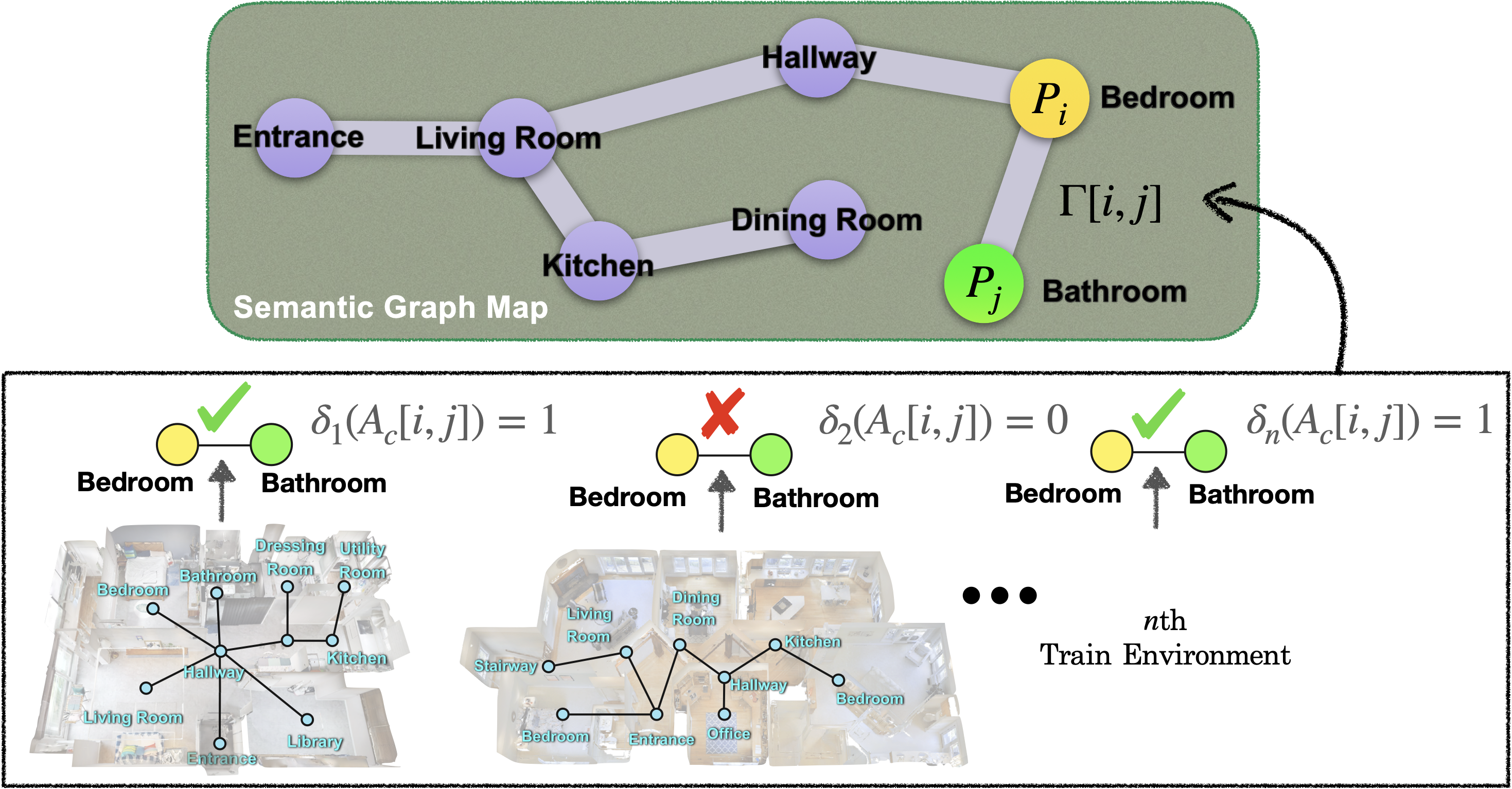
A node within the place graph represents the centroid of a place cluster, and connections between nodes signify the reachability between places. This reachability is derived from semantic graph maps collected across various training environments. If two connected image nodes, and , belong to different place clusters, and , it is inferred that the clusters are reachable. A connection between clusters in any scene sets the cluster reachability to one; otherwise, it is zero. This procedure is repeated across all training scenes, and the average value is taken as the final measure of reachability between places. The formation of the semantic graph map from episodic graphs in training environments can be shown in Figure 3. The top section of the figure shows a semantic graph map where nodes represent different rooms (e.g., Entrance, Living Room, Kitchen) and edges represent the connectivity between them. For example, the edge connects nodes (Bedroom) and (Bathroom), indicating a valid connection in the graph. In the bottom section of the figure, floor plan layouts are depicted, each demonstrating the connectivity between rooms in various training environments. In the first floor plan, the connection between the bedroom and bathroom is correctly identified (), as indicated by the green check mark. In the second training environment, the connectivity between bedroom and bathroom is not recognized (), marked by the red cross. When considering training environments, the reachability () between place cluster and is calculated as follows:
| (1) |
where and indicates the existence of a connection between place cluster and . The function denotes the presence of the place cluster in the th scene.
It is important to note that the same places are not connected, thus when . Furthermore, to normalize the reachability, we calculate it based on the number of environments in which each cluster appears, rather than the total number of environments. Reachability is set to zero if a cluster does not appear in any scene.
Place-object relationship
The relationship between object nodes and place clusters is established by connecting object nodes to image nodes within a graph, and then linking these image nodes to place graph nodes. This linkage facilitates the computation of the probability distribution for place and object categories. Specifically, for the th training environment, we calculate , where maps each object node to its corresponding object category and is the number of object categories.
By aggregating all semantic graph maps from the training environments, the relational connection between each place cluster and the object categories is defined as , where represents the number of connections between place clusters and object categories.
Given a set of object categories , the probabilities of encountering a specific place cluster given an object category , and conversely, the probability of encountering an object category given a place cluster , are computed as follows:
| (2) |
where indicates the number of connections between place cluster and object category . These probability distributions are illustrated in Section 2 of the supplementary material.

Updating relations
Our experimental setup is designed to test the navigation agent’s ability to plan its path using common sense, akin to human navigation, in a new environment without a pre-existing map. To adapt effectively to these unfamiliar settings, the SEA updates the graph in a Bayesian manner [23]. As illustrated in Figure 4, when a new place cluster or object-place connection is discovered during the construction of the semantic graph map, the prior probability is adjusted based on the new observations to calculate the posterior distribution. Given that these probabilities are determined by counting occurrences, the impact of new connections is generally minor. Thus, the update rate is set at 0.1 of the maximum count value (). The graph is continuously updated at every step. If the target object is not detected in the expected target place, the probability associated with the target object being in that place decreases. As the connection between the target object and the place cluster weakens, the next most connected place cluster is identified and explored.
3.5 Global Policy
The global policy () utilizes the RGB-D image from the directional camera () to determine subgoals () through semantic path planning, which leverages the place relationships and place-object relationships within the SEA. For example, to navigate from a bathroom to a kitchen, the calculated path might be bathroom bedroom living room kitchen. Rather than attempting to locate the kitchen directly from the bathroom, the agent first navigates to intermediary nodes such as the bedroom and the living room, thereby systematically discovering the optimal path.
Current place
To enable the semantic path planning, the agent first determines its current location by encoding RGB images and object information using the place encoder (as detailed in Section 3.2). The extracted place feature, derived from the encoded RGB image, object features, and object category, is then compared to place clusters () using cosine similarity to identify the nearest place cluster, thereby locating the agent within the environment.
Target place
The target place is chosen based on its association with the target object. The place cluster with the highest probability of containing the target object is selected as the target destination. This selection process is mathematically formulated as follows:
| (3) |
where represents the potential target place, and denotes the probability of place cluster given the target object , as defined in Section 3.4.
Subgoal place
Using conventional graph-based planning methods, a navigation agent can identify an optimal trajectory to the target place. However, the optimal subgoal may not always be near the current location. To address this, subgoal candidates are selected among the visible places identified using detected objects from the directional sensor.
To streamline the selection process and reduce computational complexity, the probability of each place, , is approximated using the importance of the object category. The object importance is defined as the inverse of the entropy of the object distribution conditioned on places, given as . Objects associated with a single place cluster have high importance, whereas those common to multiple clusters exhibit lower importance.
Among the observed objects, the category deemed most important, denoted , is used to determine the place cluster with the highest probability, calculated as . To facilitate this, the directional image with a field of view (FOV) of 120 is narrowed by 40 to focus on objects directly ahead (), to the left (), and to the right (). These selected objects help estimate the subgoal candidates: , where for representing the front, left, and right directions, respectively.
A subgoal place () with the highest reachability to the target place cluster is then chosen from these subgoal places. The selection is based on the following formula:
| (4) |
where represents the optimal semantic path from the subgoal to the target place. If a subgoal is beyond a reasonable straight-line distance, it is considered unreachable and is excluded, similar to the NRNS method [26]. The remaining candidate that is both reachable and closest to the semantic subgoal is selected as the final subgoal. If all potential subgoals belong to the same place cluster, or if no detected objects aid the decision, a subgoal is randomly chosen among them. This mechanism encourages broader exploration by the agent, preventing it from being confined to a specific area.
Furthermore, the semantic path is derived from a shortest path calculation by setting the edge weight in the place graph between th place and th place to :
| (5) |
where is a set of indices representing the optimal semantic path, starting from and ending at , the goal place. This trajectory, , represents the most probable path, effectively bridging the start and the target locations, optimizing the agent’s navigation strategy.
3.6 Local Policy
The local policy () processes directional RGB-D sensor data () along with local pose sensor readings to navigate the agent towards the designated subgoal . It employs the fast marching method (FMM) [34] to compute the shortest path from the agent’s current location to the subgoal. This computation makes use of the obstacle channel, which is derived from the top-down map created from the depth component of the RGB-D input. Upon determining the shortest path, the local policy executes a series of deterministic actions to guide the agent along this path. This strategy of navigation has been validated in previous research, demonstrating its effectiveness in various scenarios [15, 16, 21].
4 Experiments
4.1 Baselines
Non-interactive baselines
BC: A baseline for behavior cloning was trained using an RNN-based policy that takes RGB-D, agent pose, and goal object category as inputs.
End-to-end RL baselines
DD-PPO[28]: Standard end-to-end RL with distributed training over several nodes is proposed. Red-Rabbit[22]: Auxiliary tasks that improve sampling efficiency and generalization to previously unseen domains are provided. THDA [20]: RL reward and model inputs are improved, which results in better generalization to new scenes.
Metric map-based baselines
FBE[24]: A traditional frontier-based exploration method is adapted to object goal navigation using a detector to detect the target. It triggers a stop when the target is reached using the metric map. ANS[15]: A spatial metric map-based RL policy trained for exploration is adapted to the object goal navigation using the same heuristic as FBE[24] for goal detection and stopping. PONI[21]: Non-interactive training is used to navigate and only trained potential fields are used to determine the next subgoal.
Graph map-based baselines
ANS + SI[17]: An abstract model is attached to ANS[15]. The agent incrementally extends the abstract model and reuses the learned model from previous episodes. SemExp + SI[17]: An abstract model is attached to semantic exploration (SemExp[16]) using the same abstract model strategy as ANS + SI. For DD-PPO, Red-Rabbit, THDA, and PONI, publicly available MP3D results on the Habitat ObjectNav leaderboard are used. For ANS, pre-trained models released by the authors are evaluated. For ANS + SI and SemExp + SI, official results from the published paper are used.
4.2 Experimental Settings
Datasets
We utilized the Habitat simulator [1] to conduct experiments using the Matterport3D (MP3D)[27] datasets, which feature photorealistic 3D reconstructions of the real world. The standard 61 train / 11 val splits for the ObjectNav configuration, as described in Section3.1, were employed. It should be noted that only the local policy depends on the depth and pose, making the proposed method considerably more practical for use in the real world with noisy pose and depth sensors. The Habitat ObjectNav dataset [1] was used for MP3D experiments, with 21 goal categories (provided in the supplementary Section 1). We utilized 2195 episodes for the test.
Evaluation metrics
All methods were evaluated using the success rate (Success), success weighted by path length (SPL) [35], and distance to success (DTS). Success is determined by calculating the ratio of successful test episodes to the total number of test episodes. SPL takes into account both the Success and path length. When there are episodes, , where is the length of the shortest path from goal to target, is the length of the path taken by the agent, and is the binary indicator of Success for th episode. Finally, DTS is the distance (measured in ) between the agent and the success threshold (1.0) of the goal object at the end of the episode, as described in [35].
Implementation details
To construct SEA, we examined ten episodes from each train scene, for a total of 610 episodes. The maximum number of time steps was set to 500, and the environment was explored randomly. For object detection, we trained a MaskRCNN [32] model to identify 40 object categories in MP3D environments. Our method does not construct a metric map, thus a different stopping criterion was used compared to metric map-based methods. If an object is detected from a distance and exceeds a target object detection score threshold, the agent approaches the object and checks whether it is the target object. If the object detection score is lower after the encounter, it is assumed that it is not the target. The object feature with the highest detection score along the approaching path is stored in the checked object list. If a detected target object is highly similar to the checked objects, it is not rechecked, as it has already been searched. Additional details can be found in Section 1 of the supplementary material.
4.3 Results
| Method | Pose noise | MP3D (val) | ||
|---|---|---|---|---|
| Success ↑ | SPL ↑ | DTS ↓ | ||
| BC | ✗ | 3.8 | 2.1 | 7.5 |
| DDPPO[28] | ✗ | 8.0 | 1.8 | 6.9 |
| Red-Rabbit[22] | ✗ | 34.6 | 7.9 | - |
| THDA[20] | ✗ | 28.4 | 11.0 | 5.6 |
| FBE[24] | ✗ | 22.7 | 7.2 | 6.7 |
| ANS[15] | ✗ | 27.3 | 9.2 | 5.8 |
| PONI[21] | ✗ | 31.8 | 12.1 | 5.1 |
| ANS + SI[17] | ✗ | 27.9 | 13.1 | 6.1 |
| SemExp + SI[17] | ✗ | 34.7 | 15.1 | 5.8 |
| SEA (ours) | ✔ | 39.0 | 13.7 | 5.0 |
| SEA w/o Update | ✔ | 33.3 | 13.6 | 5.7 |
SEA outperforms navigation baselines
Our SEA method sets a new benchmark by surpassing all previous state-of-the-art baseline methods on the MP3D dataset’s validation split, as detailed in Table 1. This achievement encompasses end-to-end reinforcement learning (RL), metric map-based baselines, and graph map-based methods, particularly in terms of Success and DTS metrics. Remarkably, SEA demonstrates a staggering 926.3% improvement in Success compared to the behavior cloning model. Furthermore, SEA outperforms the PONI[21] by 22.64% in Success and by 13.20% in SPL, thanks to its development of more efficient pathways. While PONI[21] is highly reactive and excels in exploration with its frontier-based path generation, it falls short in exploitation; in contrast, SEA uses topological maps for long-term planning, allowing it to create more effective routes through better exploitation. When compared to the SemExp + SI[17] model, which combines an abstract model with a semantic exploration approach, SEA increases Success by 12.4%. This is particularly notable given that SEA does not use global pose information and is trained without interactive reinforcement learning. SEA outperforms SemExp[17] in terms of Success but has slightly lower SPL (by 1.4 percentage points) due to its adaptability. This adaptability allows SEA to eventually locate the object, even if it initially follows inefficient routes. In contrast, SemExp[17] relies on a highly accurate metric map and a perfect pose sensor, making it very efficient at following the optimal path. However, if SemExp[17] is led astray onto an incorrect path, it lacks the mechanism to update and correct itself, making it difficult to locate the object. SEA’s ability to adapt and correct its course enables higher success rates, even though this sometimes means taking longer and less efficient paths, resulting in lower SPL performance.
SEA has low computational requirements
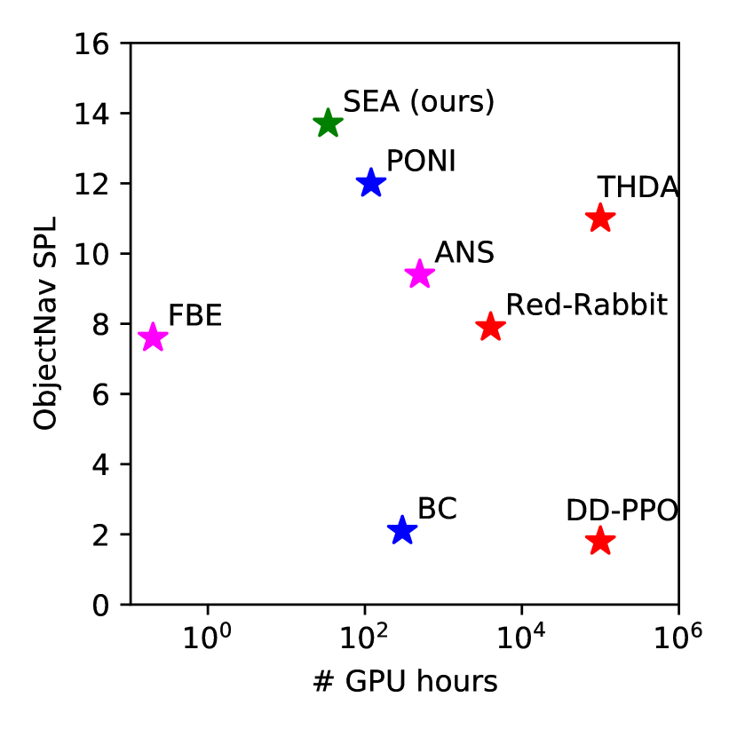
The place encoder can be trained within a day using a single GPU. Constructing SEA takes about 10 hours with a single GPU. During the inference, a GPU with 3000 MB memory is enough to run the trained encoder and detector. Our SEA has the lowest cost, three times less than the non-interactive SoTA baseline [21], as demonstrated in Figure 6.
SEA is robust to pose noises
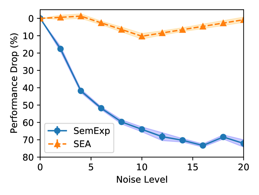
SEA demonstrates enhanced robustness to pose sensor noise by utilizing place reachability for long-term planning instead of building a metric map. As shown in Figure 6, SEA experiences a modest performance drop in Success, with a 10% decrease at a noise level of 10 and only a 0.77% reduction at noise level 20, despite significant pose sensor interference. Here, the noise levels are indicative of real-world scenarios, with noise level 1 mimicking common robotic system disturbances and higher levels representing more severe interference. In contrast, the SemExp model shows a marked decline in efficiency—42% at noise level 4 and 64% at noise level 10, further deteriorating with higher noise levels. This emphasizes SEA’s ability to maintain efficiency through consistent replanning, leveraging its global policy model effectively, even when local paths are obscured by noise. These results highlight SEA’s superior adaptability over traditional metric map-based approaches that rely on precise pose sensors.
Semantic information helps to improve localization
The accumulated graph data serves as a form of memory that integrates various pieces of semantic information. To determine whether this accumulated semantic information is indeed beneficial, we employ a trained network with attached probes to evaluate its utility for localization purposes. The localization probe network comprises Graph Neural Networks (GNNs) and transformer decoder networks. These networks are trained with the ground truth location coordinates (x, y). After training, the performance is assessed on a test set by calculating the distance between the predicted and actual locations.
Upon analyzing the localization results (Table 2, it is evident that our SEA method, utilizing inputs images (I), objects (O), and places (P), exhibits superior performance in both Acc@0.5m and Acc@1m metrics with scores of 40.4 and 73.1, respectively. The Acc@1m metric signifies the average accuracy of distance calculations within a 1-meter range. If the calculated distance is accurate within this range, an accuracy score of 1 is assigned, while inaccuracies are denoted as 0. When the performance enhancement of SEA is calculated in terms of percentage increase, we observe substantial improvements over other methods. Specifically, compared to NRNS [26], SEA demonstrates an extraordinary increase of approximately 285% in Acc@0.5m. In comparison to VGM [19], SEA shows a noticeable improvement as well. The TSGM [18] method, with inputs I and O, ranks second to SEA, yet SEA still surpasses it in terms of accuracy. To summarize, these results not only indicate the dominance of SEA in localization accuracy, particularly within a 1-meter range, but also emphasize the considerable performance enhancement achieved by incorporating semantic knowledge.
| SEA ablations | MP3D (val) | |||
|---|---|---|---|---|
| Subgoal | Stop | Success ↑ | SPL ↑ | DTS ↓ |
| ✗ | ✗ | 29.2 | 11.9 | 6.1 |
| ✔ | ✗ | 36.4 | 14.2 | 5.3 |
| ✔ | ✔ | 39.0 | 13.7 | 5.0 |
Relation update is effective on adapting to unseen environment
The effectiveness of adapting to the unseen environment through relation updates is demonstrated in the results of an ablation study presented in the second row from the bottom of Table 1. As new place connections or place-object connections arise during testing, the probability distribution is updated at each step of the current episode. This acquired connection information is utilized solely within the episode and is not stored for future use. The experiment yielded a 17.1% increase in success rate compared to the case where no episodic update was applied. Notably, SPL only improved by 0.7%. This is likely due to the episodic update altering the posterior distribution. The agent initially navigates to the location where the target object is most likely to be found and checks for its presence. If the object is not discovered in the initial place cluster, the agent may become stuck. However, the relation update weakens the connection between the target place cluster and the target object, allowing the agent to replan and reach the next most connected place cluster. As the agent successfully finds the object by moving to the next place cluster, SPL decreases as the path length of the successful path becomes longer.
Place cluster is useful for planning
We evaluated the impact of place-specific information in the planning process using a model that randomly designates subgoals. In this context, "Subgoal" refers to the place-based subgoal selection method, which strategically enhances reachability based on place connections. As delineated in Table 3, the implementation of this subgoal selection method resulted in quantifiable improvements. Specifically, success rates increased by 24.7%, and the SPL metric concurrently rose by 19.3%. The term "Stop" denotes the place-based stop mechanism, a model variant that facilitates termination before reaching the predetermined target place cluster. The examination of this mechanism revealed distinct effects. The success rate decreased by 7.1%. In conclusion, the use of place clustering proves to be advantageous for the planning process.
SEA can choose different trajectories based on different goals
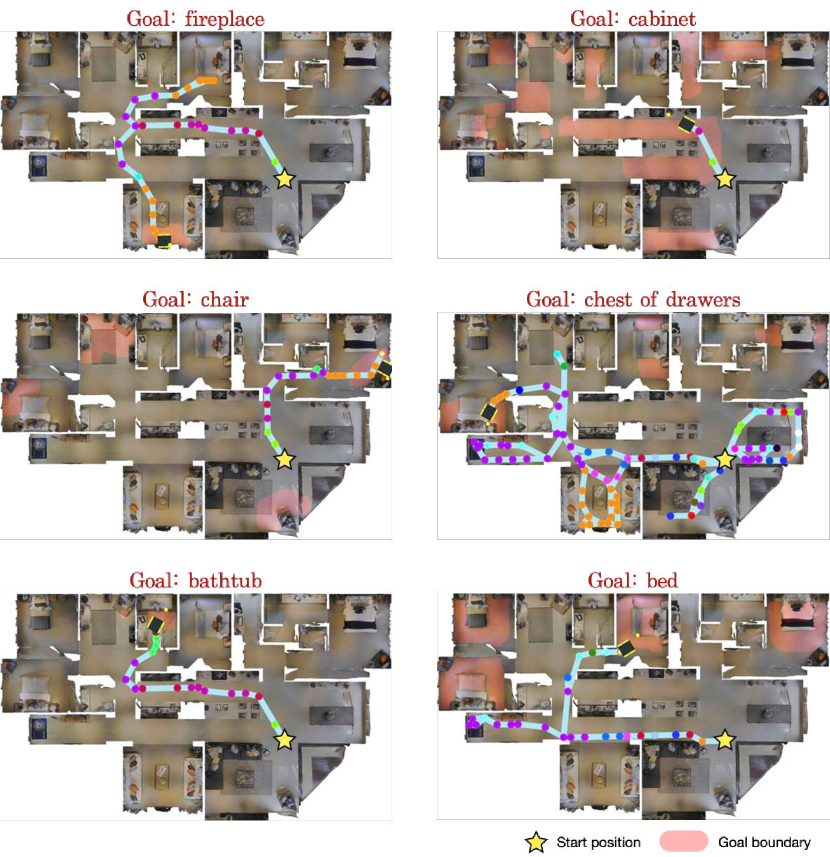
This experiment demonstrates that the path is contingent upon the chosen goal, with the starting point fixed and goal categories varied. In Figure 7, the yellow star marks the starting point, and the red region indicates the goal boundary (1m radius), solely for visualization. The figure shows trajectories for six object goals: fireplace, cabinet, chair, chest of drawers, bathtub, and bed. Each trajectory adapts to its respective target. Detailed analysis is available in the supplementary material.
5 Visualization
Construction of SGMs
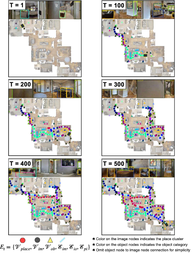
The process of constructing a SGM is depicted in Figure 8. A SGM integrates place graphs, image graphs, and object graphs. In this representation, image nodes are depicted as circles. Their colors correspond to the respective place clusters. Object nodes are depicted as triangles. The colors of these nodes indicate object categories, matching the colors of the bounding boxes in the panoramic RGB image. For clarity, connections between image nodes and object nodes have been omitted in the visualization. It is important to note that top-down maps and the positions of image and object nodes are utilized solely for visualization purposes and are not used as input data. Additionally, a supplementary video is available that demonstrates the construction of semantic graph maps, showcasing one episode across 20 training scenes.
Example visualization of episodes
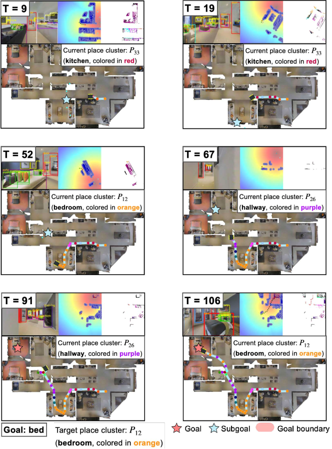
We provide an example visualization of an episode in Figure 9. This shows how semantic prior graphs are used in the global policy to perform ObjectNav, where the goal is identified as ’bed’. The navigation process begins with the agent perceiving the bedroom () to be on the left side and the kitchen to be at the front and right side. Based on this initial perception, the agent decides to move left, anticipating that the target location might be there. Upon reaching the subgoal, the agent searches for a bed but does not find one. Consequently, the agent exits the current location and re-evaluates the subgoal, noticing a door on the left and inferring that the target location is likely on the left side. While proceeding towards the subgoal, the agent eventually encounters the target object, the bed. The agent then formulates a local plan to reach the bed. Finally, after confirming that the location matches the intended destination, the bedroom (), the agent presses the stop button. Detailed information and additional examples are provided in the supplementary material.
6 Conclusions and Future Work
6.1 Conclusions
We present SEA, a method for learning semantic relationships between places and objects in unknown environments with low computational cost. Our approach identifies the object’s location and navigates using place connections. By adapting to the unseen environment through relation updates, SEA achieves state-of-the-art results for ObjectNav in MP3D. Unlike other methods are not robust to noise pose sensor, SEA is robustly navigate environment with noisy settings. Our method is the first to not require a global metric map for ObjectNav in large environments like MP3D. We show that incorporating semantic relationships improves localization and navigation tasks.
6.2 Future work
In addition to the current approach, we propose future directions and still open challenges:
1. Incorporating language features for 3D objects: Our proposed method relies solely on image features to define objects. Using language features for 3D objects could lead to more general features that can improve object search and correlation graph connections in the metric space.
2. Agents in dynamic environments: Recognizing changes in the environment, such as a cup being moved from the kitchen to the living room, can aid in task-solving. If an agent maintains memory in the form of a graph, it can adapt much better to dynamic environments compared to using a metric map.
3. Recognizing physical laws in the environment: To manipulate objects or perform meaningful control tasks, it is necessary to understand the physical laws governing the environment. For example, avoiding small wooden blocks on the floor or considering the center of mass when picking up a tool.
4. Interactive intelligence: Our method should not only rely on its own intelligence but also interact with humans or other robots in the environment to update the topological map. Further advancements in these areas can lead to more robust and effective navigation and localization in complex environments.
We believe that our proposed method is a step towards achieving this goal, and we look forward to future developments and improvements. Additional details can be found in the supplementary material.
This document provides additional information about experimental settings and includes supporting qualitative visualizations. We recommend watching our supplementary three-minute video, which showcases animated examples of navigation using SEA. Here is an overview of the sections included in the supplementary file:
Appendix A Additional Experimental Details
Implementation details
To supplement the main paper, we provide further details about the experiments. The MP3D [27] encompasses 40 object categories, while the ObjectNav dataset from the Habitat challenge contains 21 specific object categories as goals. These categories are as follows: chair, table, picture, cabinet, cushion, sofa, bed, chest of drawers, plant, sink, toilet, stool, towel, tv monitor, shower, bathtub, counter, fireplace, gym equipment, seating, and clothes. Considering some object categories in MP3D are not applicable for place-object statistics, we decided to utilize 32 specific object categories, as illustrated in Figure 13. The following eight categories were excluded: wall, floor, ceiling, column, lighting, beam, railing, misc. MP3D comprises 30 ground truth places. However, due to the ambiguity of places such as other room and junk, we opted for eight evident places for place clustering: living room, bedroom, kitchen, closet, dining room, bathroom, toilet, hallway.
Network parameters
We employed deep learning exclusively to train three encoders: the place encoder, image encoder, and object encoder. As depicted in Figures 10, 11, and 12, the encoder networks utilize ResNet18 [36] as a backbone network and include fully connected layers. For the place encoder in Figure 10, we use a single graph convolution layer for processing context of objects. For the place encoder, the maximum number of the objects are set to 10. The object features for place encoder and object encoder were extracted from images using RoI-align [32]. We utilized a stochastic gradient descent (SGD) optimizer to train the three encoders with a learning rate set at 0.03, over a total of 200 training epochs. We randomly collected 5,000 panoramic RGB images per training environment for training encoders, totaling 305,000 images. The objects were collected using a ground truth detector. We randomly selected 20,000 images as a batch for each epoch, a feasible number for -means clustering, with the mini-batch size set at 128. In training the place encoder, we specified the temperature parameter () in the clustering loss as the likelihood of an instance belonging to the corresponding cluster, following the approach in [31]. The temperature parameter () used in the metric learning was set to 0.2 for the place loss and 0.7 for the near loss. The number of negative samples () is set to 128. The number of place clusters () was set to 50, which is higher than the actual number of place labels to cover all spaces. Place features have 128 dimensions, and image feature dimension is 512 (=512). The object features have 32 dimensions (=32). is the total number of train environments, 61. For the training image encoder, which is trained in an unsupervised manner, we used near loss and cluster loss. Other parameters in the image encoder are the same as the place encoder. To make the object encoder robust to an erroneous object detector, the positive sample for training the object encoder is augmented by randomly cropping the image of objects. As mentioned in the main manuscript, the similarity thresholds for constructing image and object graphs are set to 0.8, similarly used in [19, 18].


Selecting a subgoal
Based on the current maximum depth value () of the directional camera sensor (which has a maximum depth of 5m), the local policy generates a local map. When the size of the selected local map is , subgoal candidates for a local map at away are selected. If the subgoal is beyond the straight line distance, it is considered unreachable and is eliminated, just like NRNS [26]. Subsequently, the candidate that is both reachable and closest to the selected semantic subgoal is chosen as the local goal. The local policy’s maximum number of steps is . For example, if the local policy produced a 3 3 local map, the maximum local step size is 15, whereas a 5m local map has a maximum step size of 25. If the agent reaches the local goal or exceeds the maximum step, the agent does global planning to select a new subgoal. Furthermore, if the place clusters to which subgoals belong are all the same, or if no detected objects are found, a subgoal is chosen randomly. This process facilitates greater exploration by an agent, thereby preventing it from getting stuck in a particular region.
Appendix B Illustrations of Semantic Graph Maps
B.1 Prior distributions
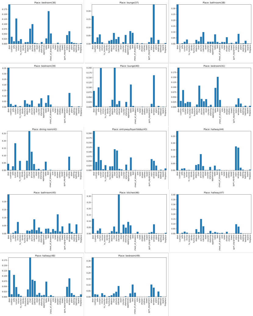
The following figures illustrate the prior distributions gathered from the semantic graph maps.
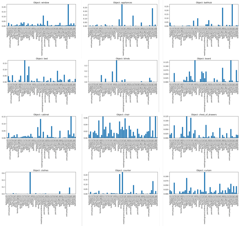
Place distribution
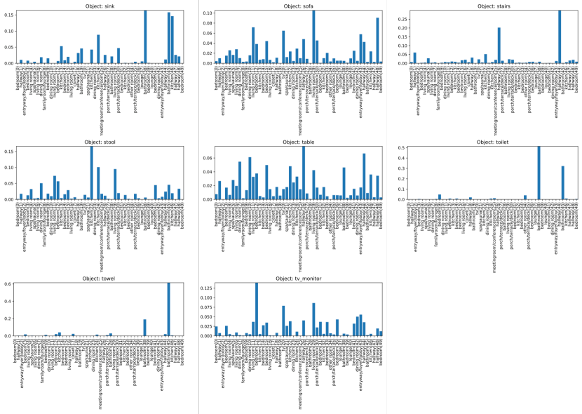
is represented in Figures 14, 15, and 16. As depicted in Figure14, beds can be located in (bedroom), (bedroom), and (bedroom) respectively. Clothes are primarily found in (closet), but can occasionally be found in (bathroom) due to the presence of shower robes. Chairs are featured in a variety of spaces. Figures15 and 16 illustrate the strong correlation between places and objects.
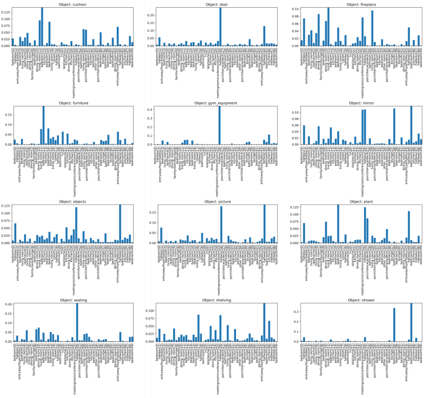
Object distribution
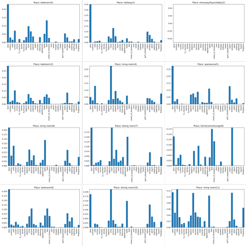
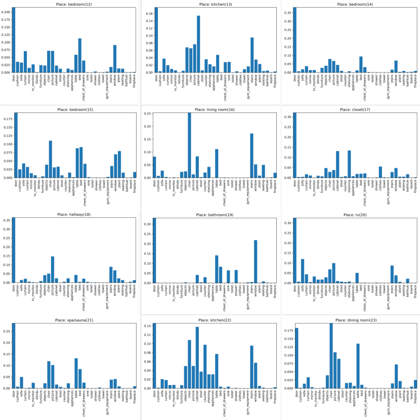
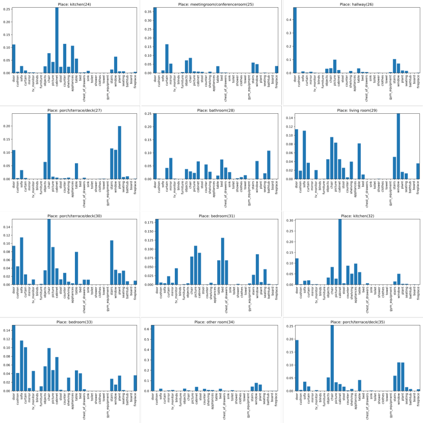
is delineated in Figures 17, 18, 19, and 20. As shown in Figure17, is absent as the episode graphs couldn’t entirely map the environment within ten episodes per scene. A better coverage of the environment could potentially enhance SEA’s performance. In Figure20, within (bedroom), the bed has the highest frequency, barring the door that is ubiquitous across all place clusters. This demonstrates that the place clusters are trained to encapsulate various locations in accordance with object distribution.
Object importance
Object categories are arranged in Figure 13 in order of their importance, defined as the inverse of the entropy of object distribution conditioned on places. The importance values are derived from the prior distribution without any updates, and may change during navigation in a test environment.
Appendix C Visualizing Place Clusters and Reachability
We provide a visualization of the place graphs from our test environment, derived purely from prior distribution and devoid of any updates.
Place clusters
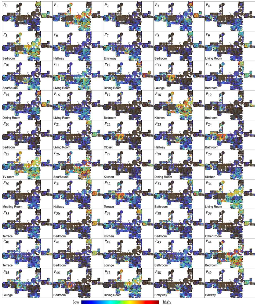
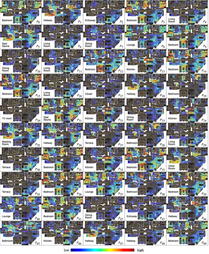
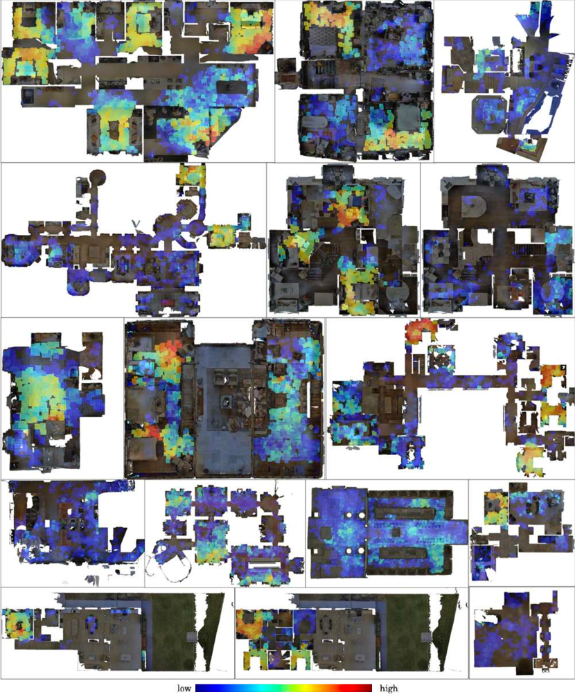
Figure 5 of the manuscript illustrates an example of a semantic path using place clusters from MP3D. We further showcase examples of these place clusters in two test scenes from MP3D, depicted in Figures 21 and 22. These particular test scenes were chosen because they possess extensive areas, diverse rooms, and complex structures. We employ RGB color-coding to represent the similarity between place clusters on the map, where red signifies high similarity and blue indicates low similarity. Maps with a similarity score less than zero are not colored, thus displaying the original top-down RGB maps. To compute the similarity between the place cluster centroid feature and the place features extracted from the map, features are gathered from 5000 random locations, as detailed in the experiment section of our main manuscript. Subsequently, the color coding serves to denote the likelihood of a place cluster’s presence at a particular location on the map. While the place names originate from the ground truth names acquired during training, the precise names of the place clusters remain undetermined. It is crucial to mention that the place features and top-down maps are employed exclusively for analytical purposes and are not accessible to the agent.
In Figure 23, we visualize the 41st place cluster () across all 16 maps, which represent the 11 test scenes, taking into account that some scenes contain multiple floors. We inferred the labels of the place clusters utilizing the ground truth place labels provided in the dataset. For instance, the 41st place cluster () is representative of a bedroom.
Place reachability
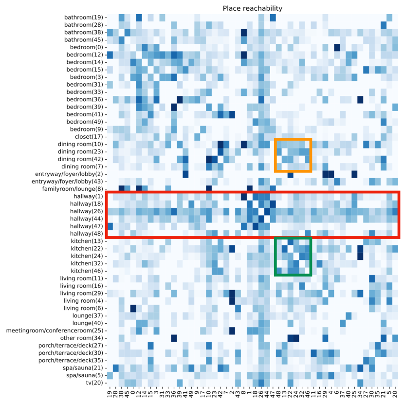
We show the reachability between place clusters in Figure 24, where the x-axis has been divided in half for visualization purposes only. The reachability is zero if the two place clusters are not connected in the episodic graph. If two place clusters are observed in the environment and are always connected, the reachability is one. As can be seen in Figure 24, the place clusters for the hallway (see red box) are linked to many other places, which means that the hallway is a bridge between places. The kitchen clusters are highly associated to other types of kitchens (green box) or dining rooms (orange box). It demonstrates that reachability is one when place clusters are adjacent and the connectivity between distant place clusters has zero reachability. The meaningful reachability values have been collected using semantic graph maps.
Appendix D Visualization of ObjectNav Episodes
Example visualization of episodes
The navigation process in Figure 7 of the main manuscript is as follow:
-
1.
Row 1. At first, the agent thinks the bedroom () is on the left side, and the kitchen is on the front and right side. The agent chooses to go to the left since the place on the left is expected to be a target place.
-
2.
Row 2. After reaching the subgoal, the agent looks for a bed, but it is not found. The agent exits the place and finds the subgoal again, and since the door is visible on the left, the agent can recognize that the target place will exist on the left.
-
3.
Row 3. Then, while going to the subgoal, the target object (bed) is found. The agent makes a local plan to reach the target object. At last, the agent presses the stop button since the place cluster matches the place searched for as the bedroom().
Please check the supplemental video for more examples.
Trajectories on different goals
Figure 8 in the main manuscript illustrates trajectories for six object goals: fireplace, cabinet, chair, chest of drawers, bathtub, and bed. The trajectories corresponding to the six target object categories display a variety of pathways, each adapted to its respective target object:
-
1.
Fireplace. The agent identifies the fireplace within the orange cluster. Initially, it searches the bedroom for the targeted object. Failing to find it in the bedroom, the agent proceeds to the next orange cluster, where it locates the fireplace.
-
2.
Cabinet. The agent recognizes that the cabinet is situated in the kitchen. It quickly locates the target by recognizing the kitchen in front of it.
-
3.
Chair. The agent discerns the presence of the chair in the orange cluster. Utilizing place reachability, it identifies the chair within the bedroom.
-
4.
Chest of Drawers. The agent encounters confusion as a chest of drawers is typically located in a bedroom (indicated by orange nodes), but in this environment, the living room contains the drawers. This discrepancy likely arises due to a mismatch between the test environment and the training environment. After some exploration, the agent successfully locates the target object, thanks to the adaptive property of the SEA.
-
5.
Bathtub. On determining that bathtubs are commonly located in bathrooms, the robot navigates its path to the bathroom, efficiently reaching the target area.
-
6.
Bed. The agent establishes that the bed is located in the bedroom. It approaches the corner of the scene via the hallway. Upon realizing there are no other rooms in the immediate vicinity, the agent proceeds to locate the bedroom elsewhere.
References
- [1] M. Savva, A. Kadian, O. Maksymets, Y. Zhao, E. Wijmans, B. Jain, J. Straub, J. Liu, V. Koltun, J. Malik, D. Parikh, D. Batra, Habitat: A Platform for Embodied AI Research, in: IEEE International Conference on Computer Vision (ICCV), 2019.
- [2] P. Mirowski, M. Grimes, M. Malinowski, K. M. Hermann, K. Anderson, D. Teplyashin, K. Simonyan, A. Zisserman, R. Hadsell, et al., Learning to Navigate in Cities Without a Map, in: Neural Information Processing Systems (NeurIPS), 2018.
- [3] K. Chen, J. P. de Vicente, G. Sepulveda, F. Xia, A. Soto, M. Vázquez, S. Savarese, A Behavioral Approach to Visual Navigation with Graph Localization Networks, Robotics: Science and Systems (RSS) (2019).
- [4] J. Yang, Z. Ren, M. Xu, X. Chen, D. Crandall, D. Parikh, D. Batra, Embodied Visual Recognition, in: IEEE International Conference on Computer Vision (ICCV), 2019.
- [5] T. Chen, S. Gupta, A. Gupta, Learning Exploration Policies for Navigation, International Conference on Learning Representations (ICLR) (2019).
- [6] A. Kumar, S. Gupta, D. Fouhey, S. Levine, J. Malik, Visual Memory for Robust Path Following, in: Advances in Neural Information Processing Systems (NeurIPS), 2018.
- [7] K. Fang, A. Toshev, L. Fei-Fei, S. Savarese, Scene Memory Transformer for Embodied Agents in Long-Horizon Tasks, in: IEEE Conference on Computer Vision and Pattern Recognition (CVPR), 2019.
- [8] N. Savinov, A. Dosovitskiy, V. Koltun, Semi-Parametric Topological Memory for Navigation, in: International Conference on Learning Representations (ICLR), 2018.
- [9] S. Gupta, J. Davidson, S. Levine, R. Sukthankar, J. Malik, Cognitive mapping and planning for visual navigation, in: IEEE Conference on Computer Vision and Pattern Recognition (CVPR), 2017.
- [10] E. Parisotto, R. Salakhutdinov, Neural Map: Structured Memory for Deep Reinforcement Learning, International Conference on Learning Representations (ICLR) (2018).
- [11] G. Avraham, Y. Zuo, T. Dharmasiri, T. Drummond, EMPNet: Neural Localisation and Mapping using Embedded Memory Points, in: IEEE International Conference on Computer Vision (ICCV), 2019.
- [12] Y. Lv, N. Xie, Y. Shi, Z. Wang, H. T. Shen, Improving Target-driven Visual Navigation with Attention on 3D Spatial Relationships, arXiv preprint arXiv:2005.02153 (2020).
- [13] H. Du, X. Yu, L. Zheng, Learning Object Relation Graph and Tentative Policy for Visual Navigation, in: European Conference on Computer Vision (ECCV), 2020.
- [14] Y. Qiu, A. Pal, H. I. Christensen, Target driven visual navigation exploiting object relationships, arXiv preprint arXiv:2003.06749 (2020).
- [15] D. S. Chaplot, D. Gandhi, S. Gupta, A. Gupta, R. Salakhutdinov, Learning to Explore using Active Neural SLAM, International Conference on Learning Representations (ICLR) (2020).
- [16] D. S. Chaplot, D. Gandhi, A. Gupta, R. Salakhutdinov, Object Goal Navigation using Goal-Oriented Semantic Exploration, arXiv preprint arXiv:2007.00643 (2020).
- [17] T. Campari, L. Lamanna, P. Traverso, L. Serafini, L. Ballan, Online Learning of Reusable Abstract Models for Object Goal Navigation, in: IEEE Conference on Computer Vision and Pattern Recognition (CVPR), 2022.
- [18] N. Kim, O. Kwon, H. Yoo, Y. Choi, J. Park, S. Oh, Topological Semantic Graph Memory for Image Goal Navigation, in: Conference on Robot Learning (CoRL), 2022.
- [19] O. Kwon, N. Kim, Y. Choi, H. Yoo, J. Park, S. Oh, Visual Graph Memory with Unsupervised Representation for Visual Navigation, in: IEEE International Conference on Computer Vision (ICCV), 2021.
- [20] O. Maksymets, V. Cartillier, A. Gokaslan, E. Wijmans, W. Galuba, S. Lee, D. Batra, THDA: Treasure Hunt Data Augmentation for Semantic Navigation, in: IEEE International Conference on Computer Vision (ICCV), 2021.
- [21] S. K. Ramakrishnan, D. S. Chaplot, Z. Al-Halah, J. Malik, K. Grauman, PONI: Potential Functions for ObjectGoal Navigation with Interaction-free Learning, arXiv preprint arXiv:2201.10029 (2022).
- [22] J. Ye, D. Batra, A. Das, E. Wijmans, Auxiliary Tasks and Exploration Enable Objectgoal Navigation, in: IEEE International Conference on Computer Vision (ICCV), 2021.
- [23] Y. Wu, Y. Wu, A. Tamar, S. Russell, G. Gkioxari, Y. Tian, Bayesian Relational Memory for Semantic Visual Navigation, in: IEEE International Conference on Computer Vision (ICCV), 2019.
- [24] B. Yamauchi, A Frontier-Based Approach for Autonomous Exploration, in: IEEE International Symposium on Computational Intelligence in Robotics and Automation (CIRA), 1997.
- [25] S. Zhang, X. Song, Y. Bai, W. Li, Y. Chu, S. Jiang, Hierarchical Object-to-Zone Graph for Object Navigation, in: IEEE International Conference on Computer Vision (ICCV), 2021.
- [26] M. Hahn, D. S. Chaplot, S. Tulsiani, M. Mukadam, J. M. Rehg, A. Gupta, No RL, No Simulation: Learning to Navigate without Navigating, in: Neural Information Processing Systems (NeurIPS), 2021.
- [27] A. Chang, A. Dai, T. Funkhouser, M. Halber, M. Niessner, M. Savva, S. Song, A. Zeng, Y. Zhang, Matterport3D: Learning from RGB-D data in indoor environments, International Conference on 3D Vision (3DV) (2017).
- [28] E. Wijmans, A. Kadian, A. Morcos, S. Lee, I. Essa, D. Parikh, M. Savva, D. Batra, DD-PPO: Learning Near-perfect PointGoal Navigators From 2.5 Billion Frames, in: arXiv preprint arXiv:1911.00357, 2019.
- [29] Z. Ravichandran, L. Peng, N. Hughes, D. Griffith, L. Carlone, Hierarchical Representations and Explicit Memory: Learning Effective Navigation Policies on 3D Scene Graphs using Graph Neural Networks, in: IEEE international conference on robotics and automation (ICRA), 2019.
- [30] M. Narasimhan, E. Wijmans, X. Chen, T. Darrell, D. Batra, D. Parikh, A. Singh, Seeing the Un-Scene: Learning Amodal Semantic Maps for Room Navigation, in: European Conference on Computer Vision (ECCV), 2020.
- [31] J. Li, P. Zhou, C. Xiong, S. C. Hoi, Prototypical Contrastive Learning of Unsupervised Representations, International Conference on Learning Representations (ICLR) (2021).
- [32] K. He, G. Gkioxari, P. Dollár, R. Girshick, Mask R-CNN, in: IEEE International Conference on Computer Vision (ICCV), 2017.
- [33] A. Vaswani, N. Shazeer, N. Parmar, J. Uszkoreit, L. Jones, A. N. Gomez, Ł. Kaiser, I. Polosukhin, Attention Is All You Need, in: Neural Information Processing Systems (NeurIPS), 2017.
- [34] J. A. Sethian, A fast marching level set method for monotonically advancing fronts, Proceedings of the National Academy of Sciences 93 (4) (1996) 1591–1595.
- [35] P. Anderson, A. Chang, D. S. Chaplot, A. Dosovitskiy, S. Gupta, V. Koltun, J. Kosecka, J. Malik, R. Mottaghi, M. Savva, , A. R. Zamir, On Evaluation of Embodied Navigation Agents, in: arXiv preprint arXiv:1807.06757, 2018.
- [36] K. He, X. Zhang, S. Ren, J. Sun, Deep Residual Learning for Image Recognition, in: IEEE Conference on Computer Vision and Pattern Recognition (CVPR), 2016.