An Innovative Attention-based Ensemble System for Credit Card Fraud Detection

Abstract

Detecting credit card fraud (CCF) holds significant importance due to its role in safeguarding consumers from unauthorized transactions that have the potential to result in financial detriment and negative impacts on their credit rating. It aids financial institutions in upholding the reliability of their payment mechanisms and circumventing the expensive procedure of compensating for deceitful transactions. The utilization of Artificial Intelligence methodologies demonstrated remarkable efficacy in the identification of credit card fraud instances. Within this study, we present a unique attention-based ensemble model. This model is enhanced by adding an attention layer for integration of first layer classifiers’ predictions and a selection layer for choosing the best integrated value. The attention layer is implemented with two aggregation operators: dependent ordered weighted averaging (DOWA) and induced ordered weighted averaging (IOWA). The performance of the IOWA operator is very close to the learning algorithm in neural networks which is based on the gradient descent optimization method, and performing the DOWA operator is based on weakening the classifiers that make outlier predictions compared to other learners. Both operators have a sufficient level of complexity for the recognition of complex patterns. Accuracy and diversity are the two criteria we use for selecting the classifiers whose predictions are to be integrated by the two aggregation operators. Using a bootstrap forest, we identify the 13 most significant features of the dataset that contribute the most to CCF detection and use them to feed the proposed model. Exhibiting its efficacy, the ensemble model attains an accuracy of 99.95% with an area under the curve (AUC) of 1.

I Introduction

The convenience of financial services for consumers around the world has been tremendously improved by digital technology. However, this development also opened up new avenues for financial fraud, especially in credit card transactions [1, 2], [3]. Criminals defraud people through various technologies and false identities intending to steal their money [4]. This gave way to a steep increase in credit card frauds as e-commerce and online shopping gained momentum [5, 6].

Looking at the numbers, one can tell that credit card fraud (CCF) is a big concern. According to Nilson’s report; global losses from card fraud amounted to 28.65 billion dollars in 2019. These figures are expected surpassing 43 billion dollars by 2025 [7, 8]. The large increase shows that fraudulent methods are getting more complicated day by day, hence making it hard to beat fraudsters at their game [9, 10]. In the United States alone, CCF cases reported to the Federal Trade Commission (FTC) were over 393 thousand during 2020, indicating a significant rise from the previous year [11, 12]. The advent of internet-based transactions worsened matters leading into rise of fraud cases involving card-not-present (CNP) transactions, which are quite common currently [1, 13]. Compared to point-of-sale fraud, the prevalence of CNP fraud rose by 81%, suggesting a major shift in digital crime [14]. This therefore means that it is necessary to propose models and techniques for detecting deceitful transactions. The old ways of identifying fraud were not quick enough [15, 16]. As a result, researchers performed thorough investigations and practically used machine learning (ML) algorithms specifically designed for CCF detection [17, 18, 19, 20].

Fraud detection extensively relies on the utilization of ML algorithms. Various ML algorithms, like support vector machine (SVM), decision tree, random forest, LightGBM, XGBoost, naïve bayes, stacking classifier and voting classifier are utilized in fraud detection [21, 22, 23, 21, 24].

Deep learning (DL) techniques were widely used in detecting fraud across fields in CCF detection. Models like Convolutional Neural Networks (CNN), Recurrent Neural Networks, and Autoencoders displayed results in spotting activities [25, 1, 26]. Hybrid models such as CNN-SVM, Autoencoder-LightGBM, ensemble method and others were commonly employed for CCF detection [27, 28, 29, 30].
Our key contributions to this research are:

• We introduce a novel fusion-based ensemble system by adding an attention layer and a selection module to the traditional stacking classifier.

• Intelligently, two aggregation operators, DOWA and IOWA, are employed to combine the predictions of first layer classifiers. In this entirely fusion-based architecture, a synergistic combination of the aggregated values by these two operators is used to feed the meta-learner.

• Dimension reduction using the bootstrap forest approach is accomplished by eliminating features that contribute negligibly to the prediction accuracy.

• The best classifiers are selected for combination based on two criteria: performance and diversity.

• The proposed model demonstrates 99.95% accuracy in detecting credit card fraud with the AUC of 1.

The rest of this paper is structured as follows: Section II introduces related work on detecting CCF. Section III first addresses the dataset and the identification of its most significant features, then introduces the aggregation operators used in the attention layer, and finally analyses the structure of the proposed system. Findings and analysis are examined in Section IV. Section V presents prospects for future studies. Finally, Section VI considers the conclusion.

II Background and Related Work

Several methodologies and algorithms were deployed to predict fraud, which saw a sharp rise in recent times. A focal area of various studies is the detection of CCF. These paragraphs delve into some of these research efforts.

Long et al. A graph network model was introduced to efficiently detect online fraud by addressing challenges such as feature disparities, category imbalances, and relationship issues [31, 32, 33, 34].

In [12], the authors proposed a CCF detection model using new transactional behavioral representations. Two time-aware gates were designed in a recurrent neural network to capture long- and short-term transactional habits and behavioral changes influenced by time intervals between transactions. The model used a time-aware attention module to extract behavioral information from historical transactions, considering time intervals, and an interaction module to enhance the learned representations. Similarly, in the realm of spotting news, LSTM and Bi LSTM methods were utilized for text data preprocessing and analysis, achieving a level of accuracy in detecting misinformation [35, 36].

Fidelis and coworkers in [37] presented a novel approach using a hybrid cultural genetic algorithm (CGA) alongside a trained modular neural network ensemble for classifying transactions. This ensemble included a complex architecture of modular neural networks, featuring components such as an encoder, selectors, a swapped recombine, swapped dynamic amplification, and a belief finisher for CGA operations. The ensemble relied on optimized rules derived from the GA-block for effective classification tasks.

Ibomoiye et al. in [38] introduced a DL ensemble method to identify CCF utilizing a mix of LSTM and gated recurrent unit (GRU) networks, as primary learners alongside an MLP acting as the meta-learner. The combined model demonstrated superior performance in sensitivity, specificity and AUC metrics when contrasted with performing GRU, LSTM and MLP models.

Within [39], the authors presented an innovative approach to detecting fraud, comprising four distinct stages. Initially, cardholders were classified into groups based on similar transaction behaviors using historical transaction data. Next, a window-sliding strategy is utilized to merge transactions in each group. Following that, distinct behavioral patterns are derived from every cardholder. Separate classifiers are trained for each group, enabling real-time fraud detection.

In [40], the authors propose the utilization of an adaptive sampling and aggregation-based graph neural network (ASA-GNN) in order to enhance transaction fraud detection. By employing a neighbor sampling strategy that selectively filters out noisy nodes and provides supplementary information for fraudulent nodes, the model effectively addresses the challenge of learning discriminative representations. To selectively choose similar neighbors with comparable behavior patterns, cosine similarity and edge weights are utilized, while introducing a neighbor diversity metric to address fraudsters’ attempts at disguise and prevent excessive smoothing.

In [41], Wang and colleagues introduced an ensemble approach that incorporates various feature ranking methods to achieve more reliable results. This method involved a two-step process: first, employing multiple rankers to create different feature rankings, and then combining these rankings using a median-based method to determine the top ten features for model building. This approach led to the development of models utilizing Decision Tree-based classifiers, specifically CatBoost and XGBoost, enhancing predictive stability and dependability.

Esenogho et al. described an ensemble classifier combining an LSTM network with the AdaBoost algorithm for efficient credit card fraud detection in [42]. Here, the LSTM serves as the base learner within AdaBoost, using data refined by the synthetic minority over-sampling technique-edited nearest neighbor (SMOTE-ENN) technique for better model training. The ensemble’s final decision was reached through a weighted voting scheme among the outcomes of various LSTM models, aiming to boost fraud detection accuracy.

In [43], the authors introduced a fresh approach to detect consumer fraud in reviews. Their method involves integrating a channel biattention convolutional neural network (CNN) with a pre-trained language model. A novel similarity computation module is introduced, which employs a metric matrix to evaluate the connection between prior knowledge and consumer reviews. This enables the model to effectively identify previously undetected fraudulent behaviors.
Although various efforts were made towards the detection and prediction of CCF, many focused on single classifiers, which are not as reliable as ensemble-based classification methods. This is because multi-classifier approaches use the consensus of several single classifiers, resulting in a more reliable outcome. Studies that examined CCF detection using ensemble classifiers either employed outdated versions such as bagging, boosting, and stacking.

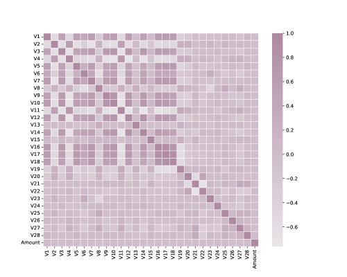
Figure 1: Heatmap of correlation matrix.

III Proposed Attention-based Ensemble System for CCF Detection

In this section, a new parallel ensemble architecture based on information fusion is introduced. This novel architecture is constructed by adding two layers to the stacking classifier structure: a) an attention layer, and b) a selection layer. Information fusion in the attention layer is accomplished through two operators, DOWA and IOWA, while the selection layer employs a mathematical logic to choose one of the two output vectors from the attention layer for each sample. Ultimately, the selected vector feeds the meta-learner.

III-A Dataset

The dataset in question includes over 550,000 anonymized records of credit card transactions performed by European cardholders in 2023 [44]. The anonymization was meticulously done to ensure the privacy and security of the cardholders’ identities. This dataset’s main purpose is to aid in creating and honing fraud detection algorithms and systems capable of pinpointing transactions that might be fraudulent. Some principal characteristics of this dataset are:

• The dataset comprises a unique identifier, named “id” assigned to each transaction for distinct identification.

• It includes anonymized features labeled V1 through V28 that encapsulate varying aspects of the transactions, such as timing and geographical details, among others, in a manner protective of user privacy.

• “Amount” denotes the monetary value of the transaction.

• there is a binary attribute named “Class” which serves the purpose of classifying transactions into two categories: fraudulent (marked as 1) and legitimate (marked as 0).

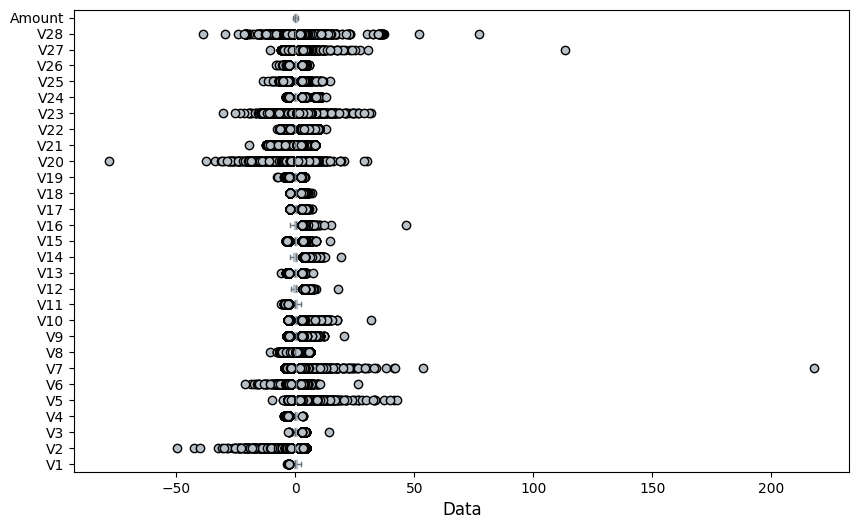
Figure 2: this boxplot visualizes the distribution of dataset features along with outliers.

Fig. 1 shows the correlation matrix, which displays the extent of linear dependencies among different features of the dataset through a heatmap. The more a cell corresponding to two features tends towards violet or white, it indicates higher linear dependencies. The boxplot in Fig. 2 Offers a graphical representation of the essential characteristics of the dataset, encompassing the median, upper and lower quartiles, and potential outliers.

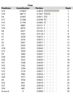
Figure 3: Predictor screening report for feature selection

III-B Predictor screening

The process of predictor screening is vital for singling out significant predictors from a broad pool of potential ones. This technique uses a bootstrap forest method to identify predictors that could impact the outcome variable.

In the analysis, a set of 100 decision trees is created using the bootstrap forest approach for each response. This model evaluates how each predictor influences the prediction of outcome. The predictors are ranked based on their contributions to the model. Fig. 3 illustrates this ranking, displaying the predictors with their corresponding contributions.

Hence, predictors whose contribution percentage falls below 0.5% are classified as insignificant dimensions. By removing these negligible dimensions from feature space $R^{29}$, we effectively transition into feature space $R^{13}$. Thus, as per Fig. 1 and Fig. 3, 16 features that have high linear or non-linear dependency on each other or are not sufficiently discriminative are removed from the raw dataset to prevent the model from becoming biased towards these uninformative features.

III-C aggregation operators

The OWA operator is a mathematical tool used for merging inputs by considering both their order and assigned weights, frequently applied in processes of decision-making and aggregation. This method systematically orders the inputs before applying specific weights to them, as highlighted in [45]. Definition 1 introduces the DOWA operator, and the IOWA operator is introduced in definition 2. These two operators are used separately to combine the predictions of first layer classifiers in subsection III-D.

Definition 1. Let $p_{1},p_{2},...,p_{n}$ represent the probabilistic outputs or forecasts from initial classifiers regarding a particular sample, indicating the likelihood of the sample’s classification into each category. Let $m$ denote the mean of these predictions across all classes, i.e., $m=\frac{1}{n}\displaystyle\sum\limits_{j=1}^{n}p_{j},\ (\alpha(1),\alpha(2),...,\alpha(n))$ is a permutation of $(1,2,...,n)$ such that $p_{\alpha(j-1)}\geq p_{\alpha(j)}$ for all $j=2,...,n$, then we call

$$c(p_{\alpha(j)},m)=1-\frac{|p_{\alpha(j)}-m|}{\sum\limits_{j=1}^{n}|p_{j}-m|},\ \ \ \ j=1,2,...,n,$$ (1)

the similarity degree between the $j$-th highest value $p_{\alpha(j)}$ and the mean value $m$.

The DOWA operator calculates the weighted mean of the predictions using a set of weights, each of which emphasizes the relevance or significance of the respective prediction. Denote by $w=(w_{1},w_{2},...,w_{n})^{T}$ the weight vector for the OWA operator, and we establish:

$$w_{j}=\frac{c(p_{\alpha(j)},m)}{\sum\limits_{j=1}^{n}c(p_{\alpha(j)},m)},\ \ \ \ j=1,2,...,n,$$ (2)

where $c(p_{\alpha(j)},m)$ is defined by (1). Clearly, we have $w_{j}\in[0,1]$ and $\sum\limits_{j=1}^{n}w_{j}=1$. Since

$$\sum\limits_{j=1}^{n}c(p_{\alpha(j)},m)=\sum\limits_{j=1}^{n}c(p_{j},m),$$ (3)

then (2) can be reformulated as

$$w_{j}=\frac{c(p_{\alpha(j)},m)}{\sum\limits_{j=1}^{n}c(p_{j},m)}.\ \ \ \ j=1,2,...,n,$$ (4)

Under these circumstances, it follows that

$$OWA(p_{1},p_{2},...,p_{n})=\frac{\sum\limits_{j=1}^{n}c(p_{\alpha(j)},m)p_{\alpha(j)}}{\displaystyle\sum\limits_{j=1}^{n}c(p_{j},m)}.$$ (5)

Using (4) weights corresponding to the predictions of each classifier are calculated. These weights can have different values for each sample. Then, the predictions of the first layer classifiers are aggregated based on the weights assigned to them by (5). This operator effectively converts the separate and independent predictions of single first layer classifiers into a single prediction.

Definition 2. The development of the weighting vector is a critical aspect widely discussed, as seen in [46, 47]. Filev and Yager proposed a method in [48] for deriving the weighting vector for an OWA aggregation through the analysis of observational data. This approach closely aligns with learning algorithms typical of neural networks, as referenced in [49, 50], utilizing the gradient descent method as its foundation. This section outlines the process for determining the OWA weighting vector’s weights based on observational input.

We are presented with a set of samples, each comprising a series of values $(p_{k1},p_{k2},...,p_{kn})$, referred to as the arguments, and a corresponding single value named the aggregated value, denoted as $d_{k}$. Our aim is to develop a model that accurately captures this aggregation process using the OWA (Ordered Weighted Averaging) method. In essence, the task is to derive a weighting vector $W$ that effectively represents the aggregation mechanism across the dataset. The aim is to determine the weighting vector $W$ based on the data provided.

The task focuses on simplifying the challenge of identifying the weights by leveraging the OWA aggregation’s linear nature with the reordered inputs. For the kth data point, the reordered arguments are signified as $b_{k1},b_{k2},...,b_{kn}$, with $b_{kj}$ being the jth largest value within the set $(p_{k1},p_{k2},...,p_{kn})$. With the arguments now ordered, the objective turns into determining the OWA weight vector $W^{T}=[w_{1},w_{2},...,w_{n}]$ in such a manner that the equation $b_{k1}w_{1}+b_{k2}w_{2}+...+b_{kn}w_{n}=d_{k}$ holds true for each instance k, from 1 up to N.

We will adjust our method by searching for a weights vector, $W$, for OWA, aiming to closely resemble the aggregating function by reducing immediate errors $e_{k}$

$$e_{k}=\frac{1}{2}\ (b_{k1}w_{1}+b_{k2}w_{2}+...+b_{kn}w_{n}-d_{k})^{2}.$$ (6)

In relation to the weights $w_{i}$, this learning challenge represents a constrained optimization issue. This is because the OWA weights $w_{i}$ must adhere to two specific criteria: $\sum\limits_{i=1}^{n}w_{i}=1$ and $w_{i}\in[0,1]$ for $i=1$ to $n$.

To bypass the restrictions, each of the OWA weights is represented in the following manner.

$$w_{i}=\frac{e^{\beta{i}}}{\sum\limits_{j=1}^{n}e^{\beta{j}}}.$$ (7)

With the transformation, regardless of the parameter values $\beta_{i}$, the weights $w_{i}$ will fall within the unit interval and their sum will equal 1. Hence, the original constrained minimization issue is converted into an unconstrained nonlinear programming problem:

Minimize the immediate errors $\textbf{e}_{k}:$

By integrating (7) into (6), it can be stated:

Motivated by the significant achievements of gradient descent methodologies in the backpropagation approach utilized for training in neural networks, we adopt it here. By applying the gradient descent technique, we establish the subsequent rule for parameter updates $\beta_{i},i=(1,n)$;

$$\beta_{i}(l+1)=\beta_{i}(l)-\alpha\frac{\partial e_{k}}{\partial\beta_{i}}|_{\beta_{i}=\beta_{i}(l)},$$ (9)

where $\alpha$ represents the rate of learning $(0<\alpha<1)$ and $\beta_{i}(l)$ signifies the approximation of $\beta_{i}$ following the lth iteration.

To simplify notation, we represent the estimate of the aggregated value $d_{k}$ as $\hat{d}_{k}$

$$\hat{d}_{k}=b_{k1}w_{1}+b_{k2}w_{2}+...+b_{kn}w_{n}.$$ (10)

Then, regarding the partial derivative $\frac{\partial e_{k}}{\partial\beta_{i}}$ we get

$$\frac{\partial e_{k}}{\partial\beta_{i}}=w_{i}(b_{ki}-\hat{d}_{k})(\hat{d}_{k}-d_{k}),\ \ \ i=[1,n].$$ (11)

Finally, we establish the formula for adjusting the parameters $\beta_{i}$ in the following manner:

$$\beta_{i}(l+1)=\beta_{i}(l)-\alpha w_{i}(b_{ki}-\hat{d}_{k})(\hat{d}_{k}-d_{k})$$ (12)

where the $w_{i}$ values are determined at each iterative step based on the current estimates of the $\beta_{i}$ values

$$w_{i}=\frac{e^{\beta_{i}(l)}}{\sum\limits_{j=1}^{n}e^{\beta_{j}(l)}},\ \ i=[1,n].$$ (13)

and $\hat{d}_{k}$ represents the current approximation of the aggregated values $d_{k}$.

This outlines the procedure implemented at each step of the iteration.

• We possess a current estimation of the $\beta_{i}$, denoted as $\beta_{i}(l)$, and a new observation composed of the ordered arguments $b_{k1},b_{k2},...,b_{kn}$ along with an aggregated value $d_{k}$.

• We utilize $\beta_{i}(l)$ to generate a current estimation for the weights

  $$w_{i}=\frac{e^{\beta_{i}(l)}}{\sum\limits_{j=1}^{n}e^{\beta_{j}(l)}}.$$ (14)

• We apply the estimated weights and the ordered arguments to derive a computed aggregated value

  $$\hat{d}_{k}=b_{k1}w_{1}(l)+b_{k2}w_{2}(l)+...+b_{kn}w_{n}(l).$$ (15)

• We update our estimations of the $\lambda_{i}$.

  $$\beta_{i}(l+1)=\beta_{i}(l)-\alpha w_{i}(l)(b_{ki}-\hat{d}_{k})(\hat{d}_{k}-d_{k}).$$ (16)

Using the 10-fold cross-validation method, we divide the predicted probabilities into two groups: test data and training data. Then, with the help of the proposed algorithm, we learn the weights from the training data, and then, using these weights and the sorted input arguments, the aggregation value is calculated for the test data.

III-D CCF detection Framework: Structure, Development, and Examination

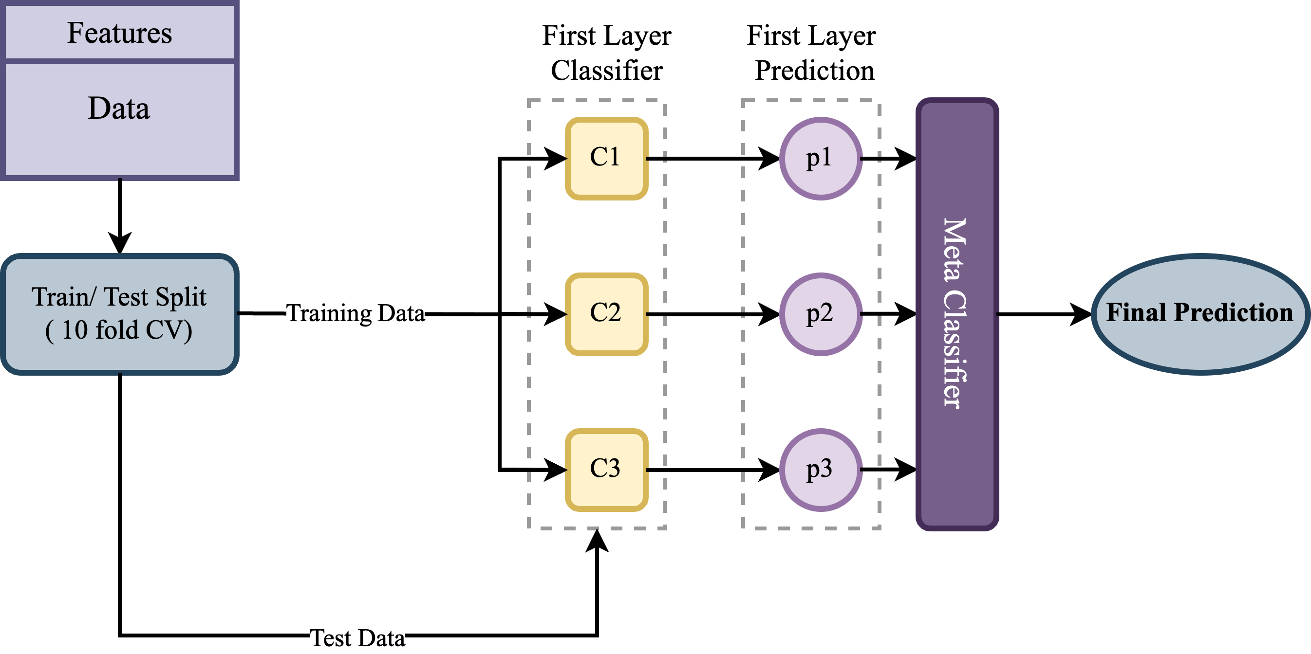
Figure 4: Traditional stacking classifier

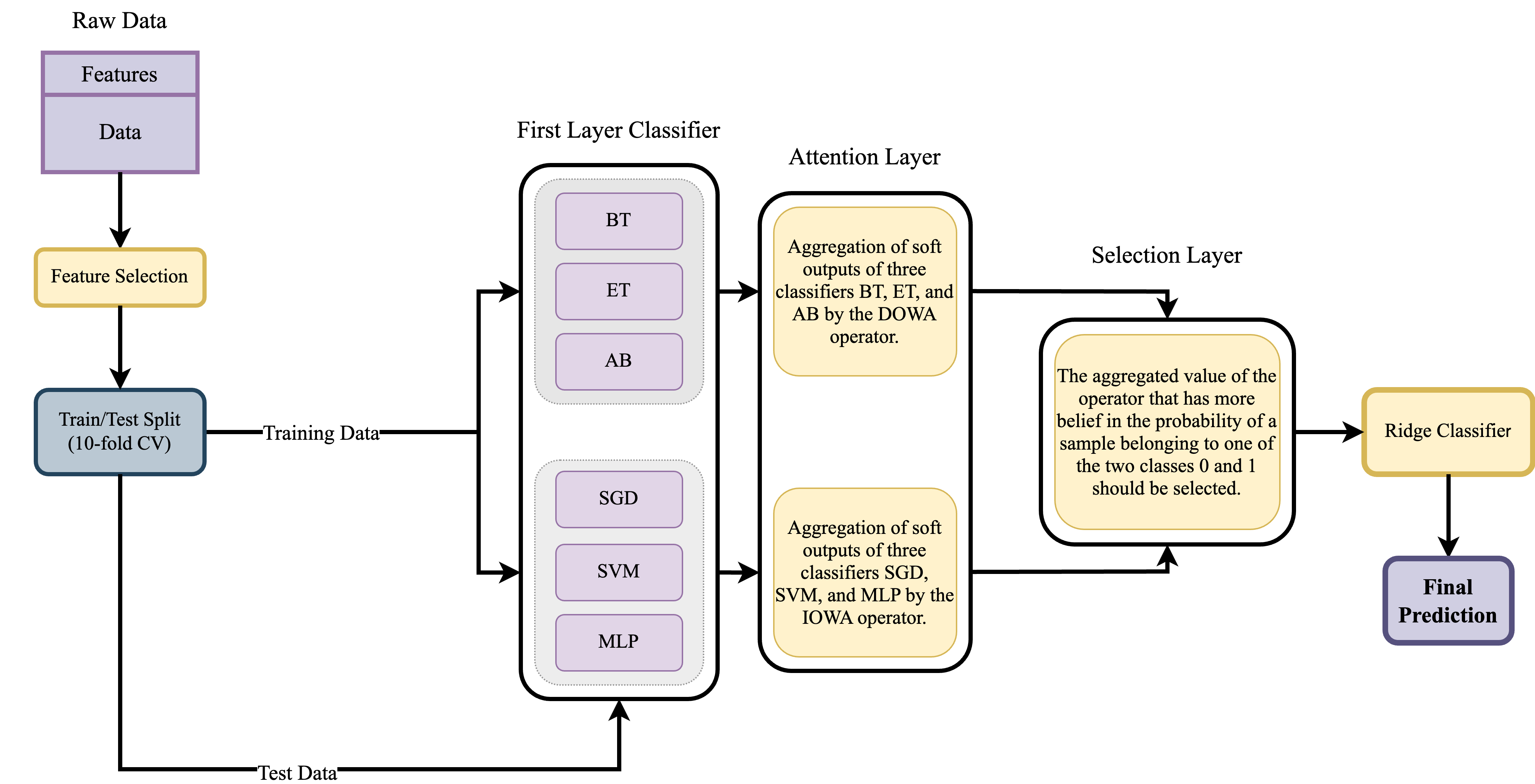
Figure 5: The block diagram of proposed architecture for detecting CCF.

Fig. 4 illustrates the structure of the traditional stacking classifier. Stacking is a method of ensemble learning that merges predictions from base models to generate a final prediction.

These base models can be of various types, including decision trees, SVM, neural networks, etc. The predictions made by these base models are then used as input features for a second-level model (or meta-learner) that aims to correct the predictions of the base models and produce the final prediction.

This study enhances the traditional stacking architecture by incorporating an attention layer and a selection layer. Fig. 5 shows the block diagram of the proposed architecture for CCF detection. In the following, we delve into the details of this entirely attention-based parallel architecture.

III-D1 First layer classifier selection

Selecting first layer classifiers is a crucial step in building an effective stacking model. The diversity and performance of these classifiers have a significant impact on the stacking model’s overall performance. Here are key considerations and strategies for selecting first layer classifiers (base models) in a stacking classifier:

Performance

Using feeble models can harm the overall performance, as they may introduce too much noise. However, models do not need to be top performers individually, as their errors might be corrected by the meta-learner. The best candidates for first layer classifiers are those not only with the best performance individually, but also whose predictions possess an acceptable level of diversity. Under these circumstances, the classifiers will complement each other well. Table I shows the 6 base classifiers that were able to meet the above criteria.

Diversity

Diverse base classifiers are crucial for making errors in different parts of the dataset. Similar classifiers lead to similar mistakes, reducing stacking effectiveness. Correlation between the predictions of first layer classifiers is a measure for assessing the level of diversity. Fig. 6 shows the correlation values between the predictions for each pair of first-level classifiers. It highlights how these two classifiers’ predictions are connected or related. This could be visualized using lines, colors, or patterns indicating areas, with medium or low correlation. High correlation areas indicate that both classifiers typically agree on sample classification, while low correlation areas suggest disagreement.

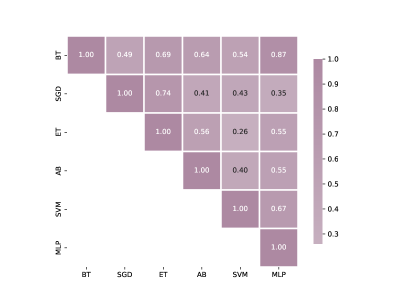
Figure 6: The correlation among the predictions generated by the classifiers in the first layer.

III-D2 attention layer

At the heart of the suggested design lies the attention layer, which allows the model to concentrate on classifiers. This layer allows the model to assign separate weightings to the predictions of each classifier based on the belief associated with each classifier. Considering the DOWA aggregation operator, which assigns a negligible weight to the classifier prediction that is an outlier compared to the other two classifiers, it is necessary for the classifiers, whose predictions are to be fused by this operator, to have sufficiently close correlations in their predictions. For example, if we assume the correlation between classifiers $C1$, $C2$, and $C3$ to be $C1C2:0.85$, $C1C3:0.9$, and $C2C3:0.4$, then by aggregating the predictions of these three classifiers using the DOWA operator, this operator will disregard the impact of one of the two classifiers, either $C2$ or $C3$, for each sample. Therefore, to employ this operator in its best performance, we select the classifiers Boosted Trees (BT), Extra Trees (ET), and AdaBoost (AB), which according to Fig. 6 have prediction correlations of 0.69, 0.64, and 0.56, respectively, which are significantly close to each other, for aggregation using DOWA. The predictions of the remaining three classifiers, namely SGD, SVM, and MLP, are aggregated using the IOWA operator.

Therefore, the weights are calculated for the three classifiers BT, ET, and AB by the DOWA aggregation operator, and for the three classifiers SGD, SVM, and MLP by the IOWA operator. Ultimately, the fusion of the probabilities assigned to each sample by the first layer classifiers is done using the calculated weights, and these probabilities are sorted in descending order. The output of the DOWA operator for each sample $i=1,2,...,N$ is a vector in the form of

$$F_{DOWA}=[f(p_{BT}^{0},p_{ET}^{0},p_{AB}^{0}),f(p_{BT}^{1},p_{ET}^{1},p_{AB}^{1})]^{T},$$ (17)

and similarly, the output of the IOWA operator is a vector in the form of

$$\small F_{IOWA}=[f(p_{SGD}^{0},p_{SVM}^{0},p_{MLP}^{0}),f(p_{SGD}^{1},p_{SVM}^{1},p_{MLP}^{1})]^{T},$$ (18)

where $p_{BT}^{0}$indicates the probability of sample i belonging to class 0 as classified by BT, and $f(p_{BT}^{0},p_{ET}^{0},p_{AB}^{0})$ represents the fused value of absolute probabilities assigned to class zero by the three classifiers BT, ET, and AB. Considering that the DOWA and IOWA aggregation operators each aggregate the soft outputs of the three specified classifiers, it can be said that each of these operators is a mapping from the space $R^{6}$ to $R^{2}$.

III-D3 selection layer

This layer receives two vectors, $F_{DOWA}$ and $F_{IOWA}$, as inputs. The basis of its operation for each sample is according to the Algorithm 1.

Algorithm 1 : Sample-Based Aggregated Value Selector

Input: $f_{i}(p_{BT}^{0},p_{ET}^{0},p_{AB}^{0})$, $f_{i}(p_{BT}^{1},p_{ET}^{1},p_{AB}^{1})$, $f_{i}(p_{SGD}^{0},p_{SVM}^{0},p_{MLP}^{0})$, $f_{i}(p_{SGD}^{1},p_{SVM}^{1},p_{MLP}^{1})$

Output: One of the aggregate values, $F_{DOWA}$ or $F_{IOWA}$, for each sample

$i\leftarrow 1$

while $i\leq N$ do

     if $|f_{i}(p_{BT}^{0},p_{ET}^{0},p_{AB}^{0})-f_{i}(p_{BT}^{1},p_{ET}^{1},p_{AB}^{1})|\geq|f_{i}(p_{SGD}^{0},p_{SVM}^{0},p_{MLP}^{0})-f_{i}(p_{SGD}^{1},p_{SVM}^{1},p_{MLP}^{1})|$ then

         return $F_{DOWA}$

     else

         return $F_{IOWA}$

     end if

     $i\leftarrow i+1$

end while

In fact, for each sample, this layer decides to intelligently select one of the two vectors, $F_{DOWA}$ or $F_{IOWA}$. The logic of selection is that whichever of the two operators, DOWA or IOWA, has greater confidence in a sample belonging to one of the two classes, 0 or 1, the aggregated value by that operator is chosen. In this way, we use a smart selection of aggregated values by both operators to feed the meta-learner. It can be said that the selection layer synergistically combines the results from these two operators.

III-D4 Meta-learner selection

The stacking process is significantly influenced by a meta-learner, as it plays a crucial role in determining the classifier’s performance. The selection of a classifier for meta learning is crucial as it directly influences the stacked ensemble’s generalization on unseen instances and, subsequently, its overall predictive accuracy. In the context of the stacking architecture, the Ridge classifier can be considered a favorable option due to its moderate complexity, which facilitates interpretability. Additionally, it incorporates regularization techniques to mitigate overfitting and effectively handles potential multicollinearity among the features used for learning. In Table II, the test results are presented, indicating that the Ridge classifier outperforms other base classifiers.

TABLE I: The degree of accuracy achieved by the first layer classifiers when evaluated on the test data.

Classifier	Accuracy
Boosted Trees (BT)	$93.64\pm 0.22\%$
Stochastic Gradient Descent (SGD)	$92.48\pm 0.13\%$
Extra Trees (ET)	$94.09\pm 0.31\%$
AdaBoost (AB)	$95.33\pm 0.19\%$
Support vector Machine (SVM)	$94.77\pm 0.25\%$
Multi-Layer Perceptron (MLP)	$95.87\pm 0.23\%$

TABLE II: Accuracy metric for choosing the meta-learner.

Learner	Accuracy
Decision Tree	$95.32\pm 0.16\%$
Gradient Boosting	$96.71\pm 0.13\%$
K-nearest Neighbor	$96.83\pm 0.11\%$
Logistic Regression	$98.44\pm 0.19\%$
Ridge Classifier	$99.95\pm 0.04\%$
CatBoost	$97.63\pm 0.19\%$

IV Findings and Analysis

In this segment, we delve deeper into the results and present a range of performance indicators to evaluate the effectiveness of the proposed algorithm. These include measures such as accuracy, sensitivity (also known as recall), precision, specificity, Matthew’s Correlation Coefficient (MCC), and the F1-Score.

IV-A Performance metrics

IV-A1 Precision

Precision quantifies the ratio of correct positive predictions to the total number of positive predictions made by a model, highlighting the accuracy of its positive predictions.

$$Precision=\frac{TP}{TP+FP}.$$ (19)

IV-A2 Specificity

Specificity measures the ratio of accurate negative predictions to the total negative predictions made by a model, underlining the precision of its negative predictions, e.g.,

$$Specificity=\frac{TN}{TN+FP}.$$ (20)

IV-A3 Accuracy

Accuracy assesses the total proportion of both true positive and true negative predictions made by a model compared to the overall number of predictions, reflecting the general reliability of the model’s predictions, e.g.,

$$Accuracy=\frac{TP+TN}{TP+TN+FP+FN}.$$ (21)

IV-A4 Sensitivity

Sensitivity quantifies the percentage of true positive instances accurately identified by a model, emphasizing the model’s capacity to detect all positive cases, e.g.,

$$Sensitivity=\frac{TP}{TP+FN}.$$ (22)

IV-A5 MCC

Unlike other metrics that may only focus on the positive class or are overly optimistic in imbalanced datasets, MCC provides a balanced measure, even if the classes are of very different sizes. MCC is defined mathematically as:

$$\small MCC=\frac{TP\times TN-FP\times FN}{\sqrt{(TP+FP)(TP+FN)(TN+FP)(TN+FN)}}.$$ (23)

IV-A6 F1-Score

The F1-score is a harmonized measure that considers precision and recall. It offers a singular metric that equilibrates the balance between precision and recall, proving valuable in situations involving datasets with imbalances, e.g.,

$$F1-Score=\frac{2\times Precision\times sensitivity}{Precision+sensitivity},$$ (24)

where $TP$ is true positive, $FP$ is false positive, $TN$ is true negative and $FN$ is false negative.

To prevent data leakage at all stages, including predictions by first layer classifiers, getting weights through a learning process by the IOWA operator, and the final prediction by the meta-learner, the 10-fold cross-validation method was used. The exceptional performance of the proposed architecture on the test data aligns with the findings reported in Table III.

Fig. 7 presents the receiver operating characteristic (ROC) curve, which showcases the correlation between the true positive rate (TPR) and the false positive rate (FPR) across different classification thresholds. The ROC curves for both classes demonstrate a significant level of overlap, suggesting comparable performance between the two classes. The ROC curve’s area under the curve (AUC) functions as a metric to assess classifier performance. A higher AUC value, approaching 1, signifies superior classifier performance. The suggested model demonstrates the AUC value of 1.

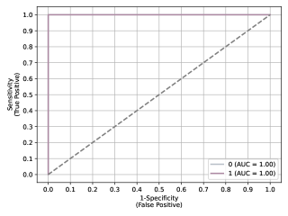
Figure 7: ROC curve along with corresponding AUC on test data.

TABLE III: Performance metrics of the proposed method.

Metric	Value
Precision	$100\%$
Accuracy	$99.95\%$
Sensitivity	$99.90\%$
Specificity	$100\%$
MCC	$99.91\%$
F1-Score	$99.94\%$

V Prospects for Future Studies

In future research, we aim to explore:

• In the proposed architecture, we randomly selected 6 classifiers as the first layer classifiers. Future work could optimize the number of first layer classifiers by relying on forward selection and backward elimination approaches.

• Future studies are recommended to focus on other aggregation methods, such as fuzzy integral operators and approaches with a higher level of complexity than OWA operators.

• There are various criteria for selecting first layer classifiers that future work could employ and compare.

• Upcoming studies could implement the suggested architecture for additional datasets that differ in terms of data origin and class balance and evaluate its performance.

VI Conclusion

The importance of detecting CCF lies in its ability to protect financial assets, maintain consumer confidence, ensure regulatory compliance, and enhance the overall security and integrity of the financial system. In this study, we introduced a novel architecture that is entirely based on integration for the detection of CCF. This architecture combines two traditional stacking architectures in parallel through the aid of two key layers including attention and selection. The attention layer utilizes two aggregation operators, DOWA and IOWA, to decide how to combine the first layer classifiers’ predictions. Each aggregation operator is tasked with combining predictions of three distinct classes. The selection layer decides which one of the two operators, DOWA or IOWA, should be considered for feeding the meta-learner for each sample, depending on which operator has more confidence in assigning the sample to one of the two classes, zero or one. This architecture, based on combining multiple classifiers, has led to improved overall accuracy, reliability, and decision-making process. This technique leverages the strengths of different classifiers and mitigates their individual weaknesses, potentially leading to more robust and accurate predictions, especially in complex or challenging classification tasks.

References

- [1] I. D. Mienye and N. Jere, “Deep learning for credit card fraud detection: A review of algorithms, challenges, and solutions,” IEEE Access, 2024.
- [2] L. Yang, B. Huo, M. Tian, and Z. Han, “The impact of digitalization and inter-organizational technological activities on supplier opportunism: the moderating role of relational ties,” International Journal of Operations & Production Management, vol. 41, no. 7, pp. 1085–1118, 2021.
- [3] S. Shibata, “Digitalization or flexibilization? the changing role of technology in the political economy of japan,” Review of International Political Economy, vol. 29, no. 5, pp. 1549–1576, 2022.
- [4] A. U. BARMO, A. HARUNA, Y. U. WALI, and K. ABID, “Analysis and comparison of fraud detection on credit card transactions using machine learning algorithms,” 2024.
- [5] B. Lebichot, W. Siblini, G. M. Paldino, Y.-A. Le Borgne, F. Oblé, and G. Bontempi, “Assessment of catastrophic forgetting in continual credit card fraud detection,” Expert Systems with Applications, vol. 249, p. 123445, 2024.
- [6] Z. Yuan, H. Chen, T. Li, X. Zhang, and B. Sang, “Multigranulation relative entropy-based mixed attribute outlier detection in neighborhood systems,” IEEE Transactions on Systems, Man, and Cybernetics: Systems, vol. 52, no. 8, pp. 5175–5187, 2021.
- [7] A. Cherif, A. Badhib, H. Ammar, S. Alshehri, M. Kalkatawi, and A. Imine, “Credit card fraud detection in the era of disruptive technologies: A systematic review,” Journal of King Saud University-Computer and Information Sciences, vol. 35, no. 1, pp. 145–174, 2023.
- [8] A. Singh, R. K. Ranjan, and A. Tiwari, “Credit card fraud detection under extreme imbalanced data: a comparative study of data-level algorithms,” Journal of Experimental & Theoretical Artificial Intelligence, vol. 34, no. 4, pp. 571–598, 2022.
- [9] P. Chatterjee, D. Das, and D. B. Rawat, “Digital twin for credit card fraud detection: Opportunities, challenges, and fraud detection advancements,” Future Generation Computer Systems, 2024.
- [10] A. Marchioni, A. Enttsel, M. Mangia, R. Rovatti, and G. Setti, “Anomaly detection based on compressed data: An information theoretic characterization,” IEEE Transactions on Systems, Man, and Cybernetics: Systems, 2023.
- [11] M. Madhurya, H. Gururaj, B. Soundarya, K. Vidyashree, and A. Rajendra, “Exploratory analysis of credit card fraud detection using machine learning techniques,” Global Transitions Proceedings, vol. 3, no. 1, pp. 31–37, 2022.
- [12] Y. Xie, G. Liu, C. Yan, C. Jiang, and M. Zhou, “Time-aware attention-based gated network for credit card fraud detection by extracting transactional behaviors,” IEEE Transactions on Computational Social Systems, 2022.
- [13] U. G. Gurun, N. Stoffman, and S. E. Yonker, “Trust busting: The effect of fraud on investor behavior,” The Review of Financial Studies, vol. 31, no. 4, pp. 1341–1376, 2018.
- [14] A. Abd El-Naby, E. E.-D. Hemdan, and A. El-Sayed, “An efficient fraud detection framework with credit card imbalanced data in financial services,” Multimedia Tools and Applications, vol. 82, no. 3, pp. 4139–4160, 2023.
- [15] K. G. Al-Hashedi and P. Magalingam, “Financial fraud detection applying data mining techniques: A comprehensive review from 2009 to 2019,” Computer Science Review, vol. 40, p. 100402, 2021.
- [16] S. Mittal and S. Tyagi, “Computational techniques for real-time credit card fraud detection,” Handbook of Computer Networks and Cyber Security: Principles and Paradigms, pp. 653–681, 2020.
- [17] A. R. Khalid, N. Owoh, O. Uthmani, M. Ashawa, J. Osamor, and J. Adejoh, “Enhancing credit card fraud detection: an ensemble machine learning approach,” Big Data and Cognitive Computing, vol. 8, no. 1, p. 6, 2024.
- [18] C. Wang, Y. Dou, M. Chen, J. Chen, Z. Liu, and S. Y. Philip, “Deep fraud detection on non-attributed graph,” in 2021 IEEE International Conference on Big Data (Big Data). IEEE, 2021, pp. 5470–5473.
- [19] Z. Li, G. Liu, and C. Jiang, “Deep representation learning with full center loss for credit card fraud detection,” IEEE Transactions on Computational Social Systems, vol. 7, no. 2, pp. 569–579, 2020.
- [20] S. Han, K. Zhu, M. Zhou, and X. Cai, “Competition-driven multimodal multiobjective optimization and its application to feature selection for credit card fraud detection,” IEEE Transactions on Systems, Man, and Cybernetics: Systems, vol. 52, no. 12, pp. 7845–7857, 2022.
- [21] Z. Zhao and T. Bai, “Financial fraud detection and prediction in listed companies using smote and machine learning algorithms,” Entropy, vol. 24, no. 8, p. 1157, 2022.
- [22] M. Valavan and S. Rita, “Predictive-analysis-based machine learning model for fraud detection with boosting classifiers.” Computer Systems Science & Engineering, vol. 45, no. 1, 2023.
- [23] M. Chen, “Credit card fraud detection based on multiple machine learning models,” in Proceedings of the 2022 6th International Conference on Electronic Information Technology and Computer Engineering, 2022, pp. 1801–1805.
- [24] K. Kowsalya, M. Vasumathi, and S. Selvakani, “Credit card fraud detection using machine learning algorithms,” EPRA International Journal of Multidisciplinary Research (IJMR), vol. 10, no. 3, pp. 109–116, 2024.
- [25] W. Wahidahwati and N. F. Asyik, “Determinants of auditors ability in fraud detection,” Cogent Business & Management, vol. 9, no. 1, p. 2130165, 2022.
- [26] Y. Lin, X. Wang, F. Hao, Y. Jiang, Y. Wu, G. Min, D. He, S. Zhu, and W. Zhao, “Dynamic control of fraud information spreading in mobile social networks,” IEEE Transactions on Systems, Man, and Cybernetics: Systems, vol. 51, no. 6, pp. 3725–3738, 2019.
- [27] T. Berhane, T. Melese, A. Walelign, A. Mohammed et al., “A hybrid convolutional neural network and support vector machine-based credit card fraud detection model,” Mathematical Problems in Engineering, vol. 2023, 2023.
- [28] H. Du, L. Lv, A. Guo, and H. Wang, “Autoencoder and lightgbm for credit card fraud detection problems,” Symmetry, vol. 15, no. 4, p. 870, 2023.
- [29] R. Cao, J. Wang, M. Mao, G. Liu, and C. Jiang, “Feature-wise attention based boosting ensemble method for fraud detection,” Engineering Applications of Artificial Intelligence, vol. 126, p. 106975, 2023.
- [30] A. S. Hussein, R. S. Khairy, S. M. M. Najeeb, and H. T. S. Alrikabi, “Credit card fraud detection using fuzzy rough nearest neighbor and sequential minimal optimization with logistic regression.” International Journal of Interactive Mobile Technologies, vol. 15, no. 5, 2021.
- [31] J. Long, F. Fang, C. Luo, Y. Wei, and T.-H. Weng, “Ms_hgnn: a hybrid online fraud detection model to alleviate graph-based data imbalance,” Connection Science, vol. 35, no. 1, p. 2191893, 2023.
- [32] P. Li, H. Yu, X. Luo, and J. Wu, “Lgm-gnn: A local and global aware memory-based graph neural network for fraud detection,” IEEE Transactions on Big Data, vol. 9, no. 4, pp. 1116–1127, 2023.
- [33] X. Hu, H. Chen, J. Zhang, H. Chen, S. Liu, X. Li, Y. Wang, and X. Xue, “Gat-cobo: Cost-sensitive graph neural network for telecom fraud detection,” IEEE Transactions on Big Data, 2024.
- [34] Y. Tang and Y. Liang, “Credit card fraud detection based on federated graph learning,” Expert Systems with Applications, p. 124979, 2024.
- [35] N. M. Reddy, K. Sharada, D. Pilli, R. N. Paranthaman, K. S. Reddy, and A. Chauhan, “Cnn-bidirectional lstm based approach for financial fraud detection and prevention system,” in 2023 International Conference on Sustainable Computing and Smart Systems (ICSCSS). IEEE, 2023, pp. 541–546.
- [36] Y. Xie, G. Liu, C. Yan, C. Jiang, M. Zhou, and M. Li, “Learning transactional behavioral representations for credit card fraud detection,” IEEE Transactions on Neural Networks and Learning Systems, 2022.
- [37] F. O. Aghware and B. Ogheneovo, “Empirical evaluation of hybrid cultural genetic algorithm trained modular neural network ensemble for credit-card fraud detection.”
- [38] I. D. Mienye and Y. Sun, “A deep learning ensemble with data resampling for credit card fraud detection,” IEEE Access, vol. 11, pp. 30 628–30 638, 2023.
- [39] C. Jiang, J. Song, G. Liu, L. Zheng, and W. Luan, “Credit card fraud detection: A novel approach using aggregation strategy and feedback mechanism,” IEEE Internet of Things Journal, vol. 5, no. 5, pp. 3637–3647, 2018.
- [40] Y. Tian, G. Liu, J. Wang, and M. Zhou, “Asa-gnn: Adaptive sampling and aggregation-based graph neural network for transaction fraud detection,” IEEE Transactions on Computational Social Systems, 2023.
- [41] H. Wang, Q. Liang, J. T. Hancock, and T. M. Khoshgoftaar, “Enhancing credit card fraud detection through a novel ensemble feature selection technique,” in 2023 IEEE 24th International Conference on Information Reuse and Integration for Data Science (IRI). IEEE, 2023, pp. 121–126.
- [42] E. Esenogho, I. D. Mienye, T. G. Swart, K. Aruleba, and G. Obaido, “A neural network ensemble with feature engineering for improved credit card fraud detection,” IEEE Access, vol. 10, pp. 16 400–16 407, 2022.
- [43] S. Lai, J. Wu, C. Ye, and Z. Ma, “Ucf-pks: Unforeseen consumer fraud detection with prior knowledge and semantic features,” IEEE Transactions on Computational Social Systems, 2024.
- [44] “Credit card fraud detection 2023, retrieved from kaggle repository on 18.04.2023, https://www.kaggle.com/datasets/nelgiriyewithana/credit-card-fraud-detection-dataset-2023.”
- [45] M. H. Chagahi, S. M. Dashtaki, B. Moshiri, and M. J. Piran, “Cardiovascular disease detection using a novel stack-based ensemble classifier with aggregation layer, dowa operator, and feature transformation,” Computers in Biology and Medicine, p. 108345, 2024.
- [46] R. R. Yager and N. Alajlan, “Some issues on the owa aggregation with importance weighted arguments,” Knowledge-Based Systems, vol. 100, pp. 89–96, 2016.
- [47] S. M. Dashtaki, M. Alizadeh, and B. Moshiri, “Stock market prediction using hard and soft data fusion,” in 2022 13th International Conference on Information and Knowledge Technology (IKT). IEEE, 2022, pp. 1–7.
- [48] D. Filev and R. R. Yager, “On the issue of obtaining owa operator weights,” Fuzzy sets and systems, vol. 94, no. 2, pp. 157–169, 1998.
- [49] A. Khaled, K. Mishchenko, and C. Jin, “Dowg unleashed: An efficient universal parameter-free gradient descent method,” Advances in Neural Information Processing Systems, vol. 36, pp. 6748–6769, 2023.
- [50] Y. Wang, Y. He, and Z. Zhu, “Study on fast speed fractional order gradient descent method and its application in neural networks,” Neurocomputing, vol. 489, pp. 366–376, 2022.