Evaluating Cooling Center Coverage Using Persistent Homology of a Filtered Witness Complex

Abstract

In light of the increase in frequency of extreme heat events, there is a critical need to develop tools to identify geographic locations that are at risk of heat-related mortality. This paper aims to identify locations by assessing holes in cooling-center coverage using persistent homology, a method from topological data analysis. Methods involving persistent homology have shown promising results in identifying holes in coverage of specific resources. We adapt these methods using a witness complex construction to study the coverage of cooling centers. One standard technique for studying the risk of heat-related mortality for a geographic area is a heat vulnerability index (HVIs) based on demographic information. We test our topological approach and an HVI on four locations (central Boston, MA; central Austin, TX; Portland, OR; and Miami, FL) and use death times of connected components and cycles to identify most at risk regions. PH and HVI identify different locations as vulnerable, thus showing measures of coverage need to extend beyond a simple statistic. Using persistent homology along side the HVI score identifies a complementary set of regions at risk, thus the combination of the two provide a more holistic understanding of coverage.

55N31, 91D20, 91B18, 86A08

1 Introduction

The Environmental Protection Agency has identified extreme heat as the modern leading cause of weather-related mortality in the United States [11]. The problem of heat-related mortality is expected to remain a pressing concern, especially if proactive measures are not adopted. Meehl and Tebaldi’s global coupled climate model showed that heat waves in North America are projected to intensify, occur more frequently, and persist longer in the latter half of the 21st century [25]. This escalation in heat intensity is linked to rising levels of greenhouse gases. There is evidence that the warmest day of the year will increase by 4-6°C (7.2-10.8°F) by the end of the century [29]. Heat accumulation is expected to be greater in urban areas due to human activity and construction, a phenomena coined “the urban heat island effect” [34]. The increase in temperature presents a major health hazard.

Exposure to extreme heat can result in dire health outcomes including heat stroke, the exasperation of existing medical conditions, permanent neurological damage, and, in the worst cases, loss of life [3]. In particular, children and seniors are at a greater risk as they have increased difficulty adapting to heat [16]. Therefore, there is a critical need to develop tools to help locate populations most vulnerable to heat-related mortality. Often, the term“excess deaths” is used when reporting the quantity of heat-related fatalities as they are often preventable. For instance, a single heat-wave event in Europe resulted in approximately 22,000-45,000 excess deaths in 2003 [3].

In a study that aimed to identify protective measures against heat-wave related deaths, Bouchama found that visiting air conditioned environments was strongly associated with better health outcomes [3]. In fact, the meta-analysis showed that those who visited air conditioned places had an approximately 66% lower likelihood of heat-related mortality. However, approximately 28.6% of housing units in the United States do not have air conditioning [24]. Furthermore, certain populations are more likely to lack air conditioning due to limited financial and social resources [24]. Therefore, it is important for cities to offer free, accessible, public cooling spaces during extreme heat events. Cooling centers can include buildings such as libraries, community centers, and senior centers [24]. It is imperative not only to increase the quantity of cooling centers but also to strategically position them in areas of highest necessity, taking into account factors such as the demographics within the city and existing cooling center locations. Currently, as Kim addresses, the distribution of cooling centers is not always optimized to maximize access [24]. Altogether, these findings motivate our emphasis on studying the geographic distribution of cooling centers within cities in the United States.

1.1 Related Work and Contributions

Currently, a variety of computational tools exist to evaluate a region’s cooling center coverage. One technique to evaluate coverage is the catchment area method which involves selecting a cut-off distance and evaluating who is within that distance of a given cooling center [24, 27]. However, this approach alone overlooks important demographics that may helpful in determining areas of greatest risk. For instance, a neighborhood of primarily senior citizens with little tree canopy may need to be treated differently than other neighborhoods. To account for this, many studies compute a social vulnerability index for a given geographic area based on demographic variables that influence an individual’s ability to overcome environmental hazards [8]. In the context of extreme heat risk, they are often called heat vulnerability indices (HVIs). There are multiple methods to calculate a region’s HVI [4]. Some previous studies utilize a combination of HVI maps and geospatial statistics to inform a maximal coverage location problem, that is, finding the optimal locations for new cooling centers. For example, the GIS Network Analyst tool, which optimizes road networks, has been used in conjunction with HVI data to recommend optimal locations for future cooling centers [4, 15]. This approach, however, lacks interpretability since one of the algorithms used has some built-in heuristics that are not transparent to the user.

A tool from topological data analysis (TDA), persistent homology (PH), provides a complementary perspective to these existing techniques. Firstly, TDA can evaluate coverage across a range of parameter values which bypasses the arbitrary selection of a cut-off distance. Secondly, many traditional methods, such as those that rely solely on the information provided by an HVI map, treat each census block as an isolated “island” when assessing the risk of its residents. For example, a single census block without cooling centers within its borders might be deemed highly at risk using conventional methods. In contrast, PH is able to incorporate spatial information by considering cooling centers in neighboring census blocks. Therefore, PH can analyze the surrounding areas and determine that the risk may be lower than it appears due to the abundant cooling centers in a neighboring block, for example. Lastly, our methodology considers cooling centers not only within city limits, but also in neighboring cities. In reality, during an extreme heat event, individuals who live on the boundary of a given city have the option of traveling to neighboring cities to find shelter.

Persistent homology has shown success in many applications to spatial data [19, 12, 20, 13, 7]. Our method is inspired by that of Hickok et al. [19] which uses TDA to infer holes in voting site coverage. However we use a different construction of the mathematical representation of space. In particular, we use a witness complex while the authors of Hickok et al. [19] use a weighted Vietoris–Rips complex.

1.2 Organization of this paper

In Section 2 we introduce the relevant background information on persistent homology. In Section 3, we present two methodologies, one based on persistent homology and the other an HVI for comparison. We present and analyze the results in Section 4 and conclude with discussions of implications and limitations of our work in Section 5

2 Background

Here we present a brief overview of topological data analysis and, in particular, persistent homology. We first begin with some preliminary definitions in Sec. 2.1, followed by an introduction to persistent homology in Sec. 2.2. We point the interested reader to [9] for a more formal treatment of this material.

2.1 Definitions

A simplicial complex is a shape constructed from lower dimensional building blocks such as vertices ($0$-simplices), edges ($1$-simplices), triangles ($2$-simplices), and higher dimensional analogs. In general, a $k$-simplex $\sigma$ is the convex hull of $k+1$ linearly independent points. A face $\tau$ of a simplex $\sigma$ is the convex hull of a subset of the points in $\sigma$; if $\tau$ is a face of $\sigma$ we write $\tau\subseteq\sigma$. A simplicial complex $\mathcal{K}$ is a set of simplices that satisfy two conditions: (1) $\mathcal{K}$ is closed under taking faces (i.e., if $\sigma\in\mathcal{K}$ and $\tau\subseteq\sigma$ then $\tau\in\mathcal{K}$) and (2) $\mathcal{K}$ is closed under intersections (i.e., if $\sigma_{1},\sigma_{2}\in\mathcal{K}$ then $\sigma_{1}\cap\sigma_{2}\in\mathcal{K}$). A filtered simplicial complex is a simplicial complex $\mathcal{K}$ and a function $f:\mathcal{K}\to\mathbb{R}$ such that $f(\tau)\leq f(\sigma)$ for $\tau\subseteq\sigma$.

From a filtered simplicial complex, one can build a nested sequence of simplicial complexes

(1) $$\mathcal{K}_{\alpha_{0}}\subseteq\mathcal{K}_{\alpha_{1}}\subseteq\cdots\subseteq\mathcal{K}_{\alpha_{n}}\,,$$

where $\alpha_{0}<\alpha_{1}<\cdots<\alpha_{N}$ and $\mathcal{K}_{n}=\{\sigma\in\mathcal{K}:f(\sigma)<\alpha_{n}\}$. Equation 1 defines a filtration. We call $\alpha$ the filtration parameter.

The first step in computing the “shape” of data is to first represent the data as a (filtered) simplicial complex. This can be done in numerous ways including common approaches such as a Čech or Vietoris–Rips complex [9]. Here we use a witness complex because it allows for the incorporation of two sets of points, the landmarks $L$ and the witnesses $W$ [32]. Often the landmarks are chosen as a subset of the witnesses so the resulting complex has fewer simplices than a Vietoris–Rips complex. However, this is not a requirement. The landmarks form the vertices of the simplicial complex and witnesses are used to determine which higher dimensional simplices are present. The landmarks form the $0$-simplices and a $k$-simplex for $k>0$ is in the complex if it is “witnessed” by a point in $W$. This “witness” relation can be defined in different ways to create variants such as a weak or strong witness complex [32, 1, 31]. We define a filtered witness complex as a witness complex paired with a filter function $f:\mathcal{W}\to\mathbb{R}$ where $f(\sigma)$ is the distance from $\sigma$ to its witness. From this, a filtration can be built by following the same construction as defined in Eqn. 1. We define our construction of the witness complex in detail in Section 3.1.

2.2 Persistent Homology

Homology is an invariant from algebraic topology used to quantify holes in different dimensions. A 0-dimensional (0D) hole represents a connected component and a 1-dimensional (1D) hole represents a cycle or a loop. Given a simplicial complex, one can compute homology; given a filtration, one can compute persistent homology. At each step in the filtration, connected components may appear and merge, and holes may form and fill in. A component or a hole is said to be born in the first step of the filtration in which it appears. A component is said to have died when it merges with another connected component, while a hole dies when it is filled in. More formally, the birth time of a homology class is $\alpha_{b}$ if the the homology class appears in $\mathcal{K}_{\alpha_{b}}$ but not $\mathcal{K}_{\alpha_{i}}$ for $i<b$. Similarly, the death time of a homology class is $\alpha_{d}$ for $d>b$ if the homology class is present in $\mathcal{K}_{\alpha_{d-1}}$ but not in $\mathcal{K}_{\alpha_{d}}$. When two components merge, the older (i.e. the one born earlier) persists while the younger dies; this is known as the elder rule [10]. The birth simplex is the first simplex that creates a homology class, while the death simplex is the last simplex added that kills the homology class.

Persistent homology results in a persistence diagram, a multiset of points where a homology class that is born at $b$ and dies at $d$ is represented by the point $(b,d)$. Since death times are always greater than birth times, all points in the persistence diagram fall above the line $b=d$.

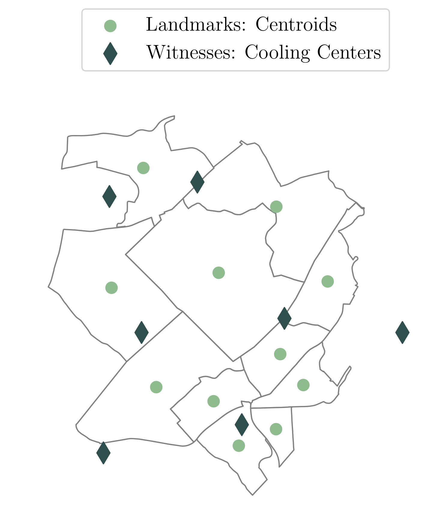
Figure 1: An example of a distribution of 11 census tract centroids (landmarks) and randomly generated cooling centers (witnesses). Note: this image was created based on a small subset of Boston, MA census tracts. Our results on Boston, MA as presented in Section 4 use census block centroids (landmarks) and OpenStreetMap cooling centers (witnesses).

3 Methods

In this section we present two methodologies for evaluating cooling center coverage. Section 3.1 introduces our topological approach using persistent homology of a filtered witness complex to identify the vulnerable locations. Subsequently, Section 3.2 defines a heat vulnerability index (HVI), inspired by existing literature. We use this more standard approach to studying vulnerability as a comparison to the topological approach. Note that our topological approach uses census blocks, however due to the availability of demographic data, the HVI score can only be computed for census tracts.

3.1 Our Construction of the Witness Complex

The witness complex is a simplicial complex constructed based on two sets of points: landmarks, $L=\{\ell_{i}\}$, and witnesses, $W=\{w_{j}\}$. We will construct it as follows:

Definition 3.1.

Let $L$ be the set of landmark points, $W$ be the set of witness points, and $\alpha\in\mathbb{R}^{\geq 0}$ be a scale parameter. We define the witness complex constructed from $L$ and $W$ at scale $\alpha$ as follows:

$$\mathcal{W}(L,W)_{\alpha}=\{ \sigma:\text{ for all pairs of 0-faces }\ell_{i},\ell_{j}\in\sigma,\text{ there exists some }w\in W$$

$$\text{ such that }d(\ell_{i},w)\leq\alpha\text{ and }d(\ell_{j},w)\leq\alpha\}$$

where $d(\ell,w)$ is the distance between landmark $\ell$ and witness $w$.

Intuitively, this is a simplicial complex constructed with landmarks as the vertices (all of which are born at $\alpha=0$), and simplices built from the sets of vertices contained within distance $\alpha$ from the same witness. Note that this construction is a clique complex; that is, if all faces of a simplex are in the complex, the face is included as well. Given an increasing set of $\alpha$ values

$$0<\alpha_{0}<\alpha_{1}<\alpha_{2}<\cdots<\alpha_{n}$$

then the sequence of simplicial complexes

$$\mathcal{W}(L,W)_{\alpha_{0}}\subseteq\mathcal{W}(L,W)_{\alpha_{1}}\subseteq\mathcal{W}(L,W)_{\alpha_{2}}\subseteq\cdots\subseteq\mathcal{W}(L,W)_{\alpha_{n}}$$

defines a filtration.

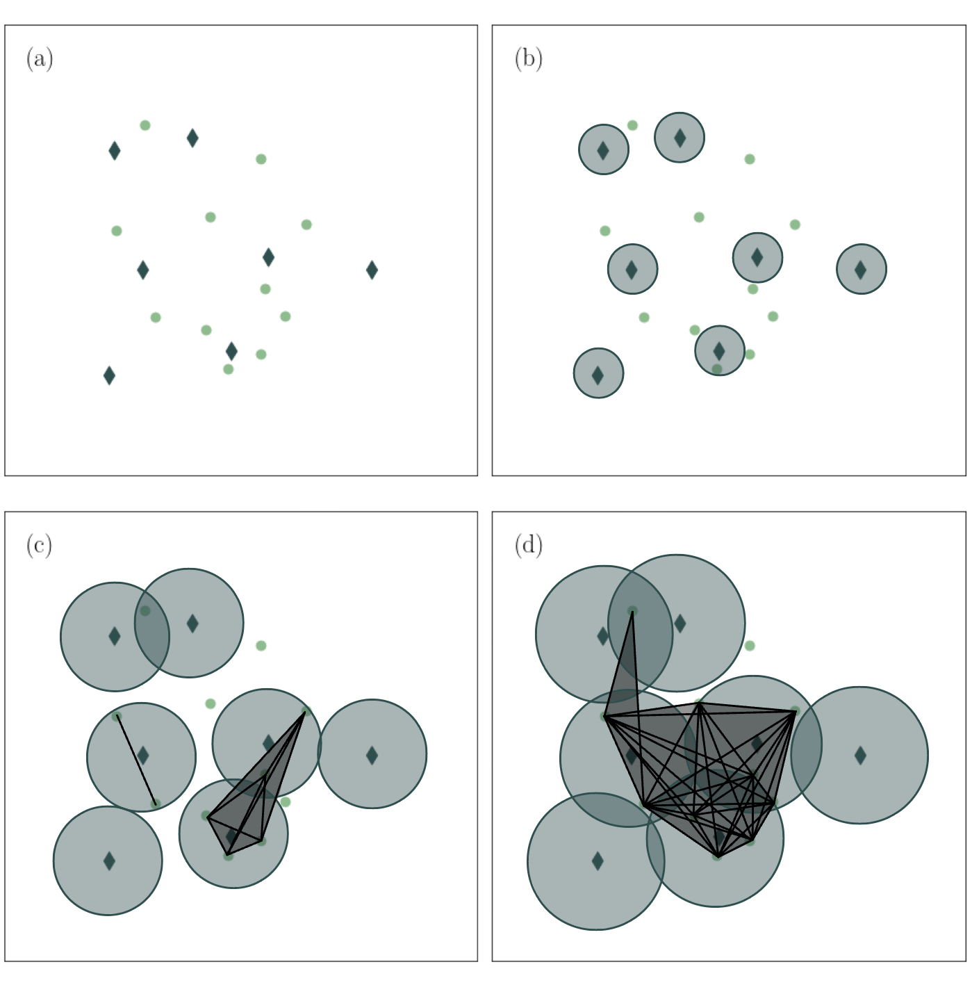
Figure 2: Example of select steps in the filtration. As shown in Figure 1, light green points represent the centroids (landmarks) of the geographic region and dark green diamonds (witnesses) represent the cooling center locations. All vertices (landmarks) appear in (a). (b)-(d) show the simplicial complex (in black) at various stages of the filtration. Edges are drawn between vertices when they are within a distance $\alpha$ of the same witness. Green discs show the radii at that filtration value. Note that the witnesses are draw for easier visualization but they are not vertices in the simplicial complex.

For this application, we use the centroids of census blocks as the landmarks, and the locations of cooling centers as the witnesses, refer to Figure 1 as an example. This means, in the filtered witness complex, an edge is added between two landmarks when the corresponding census blocks are both within distance $\alpha$ of the same cooling center. See Figure 2 as an example of how components evolve over select steps in a filtration. When two landmarks are connected by an edge, in other words, when they have access to the same cooling center, we interpret this as the two census blocks having “equal coverage.”

Given that each city is in a different region of the country, computing distances like a Euclidean distance on a projected map of the US may distort the distances in some cities more than others. To avoid the distortion of projected maps, we compute distances between latitude and longitude points using the shortest arc length or geodesic distance. We believe this choice to be justifiable because some studies have shown straight-line measurements are an acceptable proxy to travel distances in urban areas [2, 14, 22]. Furthermore, in non-emergency situations, Boscoe et al. concluded that the difference between straight-line and driving estimates were inconsequential and, because of this, straight-line estimates are often used [14, 27]. This measure of distance is then converted into units of kilometers for easier interpretation.

Details on the data we use can be found in Appendix A.1 and A.2. Our code for constructing the witness complex can be found on GitHub. We use the GUDHI library [30] for computing persistent homology.

3.2 Our Heat Vulnerability Index Score

To test our method against more standard approaches in this field, we compute a heat vulnerability index (HVI). This is based on characteristics of the demographics and environment that have been shown to exacerbate the likelihood that a person will suffer negative health consequences from an extreme heat event. Due to data availability, this score is defined on census tracts, not census blocks. The characteristics of a census tract $T$ that we use are the typical afternoon temperature $F(T)$ in Fahrenheit, the percentage of the area not covered by tree canopy $C(T)$, and the number of younger and older residents, $Y(T)$ and $S(T)$ respectively. The HVI score $V(T)$ of census tract is

(2) $$V(T)=\frac{F(T)-\mu_{F}}{\sigma_{F}}+\frac{C(T)-\mu_{C}}{\sigma_{C}}+\frac{Y(T)-\mu_{Y}}{\sigma_{Y}}+\frac{S(T)-\mu_{S}}{\sigma_{S}}\,,$$

where $\mu_{F}$ is the mean and $\sigma_{F}$ is the standard deviation of temperatures across all census tracts within a given city (other variables are defined analogously). This unweighted $z$-score approach is modeled after other HVI computations [5, 6, 21]. We standardize the variables before creating a composite score to account for their differing units of measurement.

Various factors influence an individual’s risk of heat-related mortality. Our motivation for incorporating these four variables into our measure of vulnerability is detailed as follows. Firstly, one can imagine that a warmer census block with few trees may not fare well during an extreme heat event. Secondly, being over the age of 65 puts an individual more at risk of heat related mortality due to social isolation and a lack of mobility to get assistance when faced with emergencies [16]. Lastly, because children thermoregulate less effectively than adults, they are more likely to respond poorly during extreme heat events [16]. The census block is interpreted to be at greater risk when its HVI score is higher. See Figure 3 for the maps of HVI scores across the four regions of interest. Cutter et al. explains that an essential component of building a HVI score involves testing for multicollinearity among demographic variables [8]. We verified that the four variables used in this study are independent using variance inflation factor (VIF). More details on the demographic data used to create the HVI score can be found in Appendix A.3. Refer to Table 2 for the results of the VIF analysis.

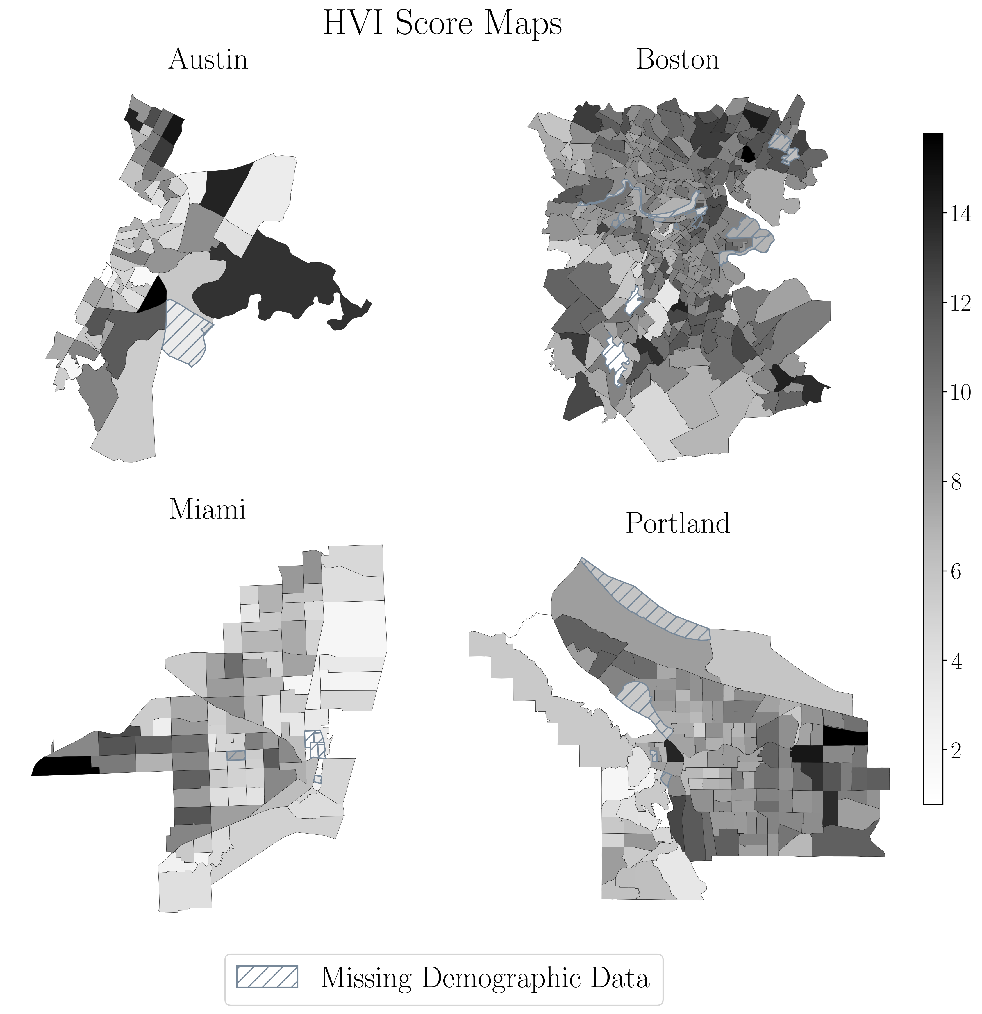
Figure 3: Heat vulnerability index (HVI) score maps for the four regions of interest. Hatching highlights census tracts that had one or more missing data value(s) for typical afternoon temperature, area not covered in by tree canopy, the number of younger residents, or the number of older residents.

4 Results

We test our methodology on four locations in the United States that offer unique climates and demographics. Those locations include central Boston, MA; central Austin, TX; Portland, OR; and Miami, FL. These cities differ in various ways, for example Miami and Boston are on the water, while Austin is landlocked. Additional differences include humidity, which can increase how warm a temperature feels, and the populations of vulnerable demographics such as older adults. It is important to note that all the selected cities are vulnerable to the urban heat island effect [26]. In the context of our data, we are able to deduce which census blocks (landmarks) in our simplicial complex remain disconnected from other census blocks for a longer duration. This can be interpreted as more “vulnerable” as they are further away from cooling centers compared to other census blocks. We compute the PH of the filtered witness complex for each of the four locations of interest. Their persistence diagrams (PDs) are shown in Figure 4. Notably, the PD for Boston shows significantly more 1D homology class points than any other location.

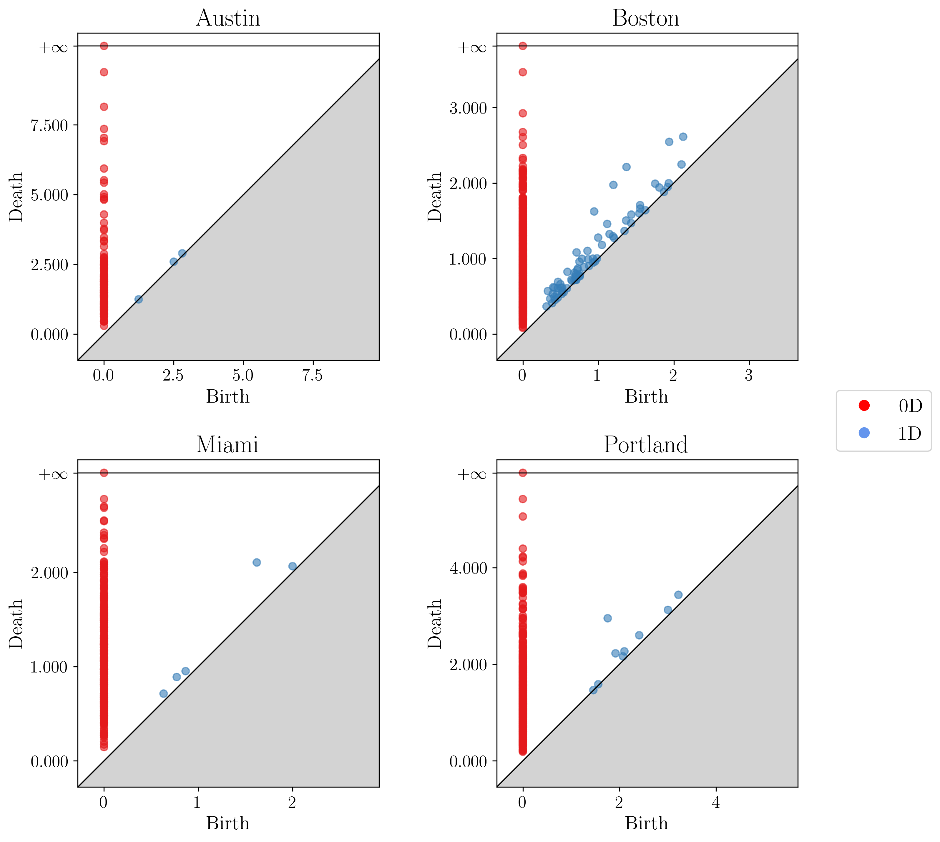
Figure 4: Persistence diagram for our four geographic locations. Note that the axes are not on the same scale.

Figure 5 maps the death simplices of the 0D homology group for our four geographic locations. Those with larger death values are interpreted as connecting one region to one with higher risk of heat-related mortality. For instance, the southern tip of Austin (census tract 24.32) has an especially large death time. Other high death values can be observed in the south-east area of central Boston, on the northern (coastal) tip and south-west (coastal) edge of Miami, and the north-west and south-east tip of Portland.

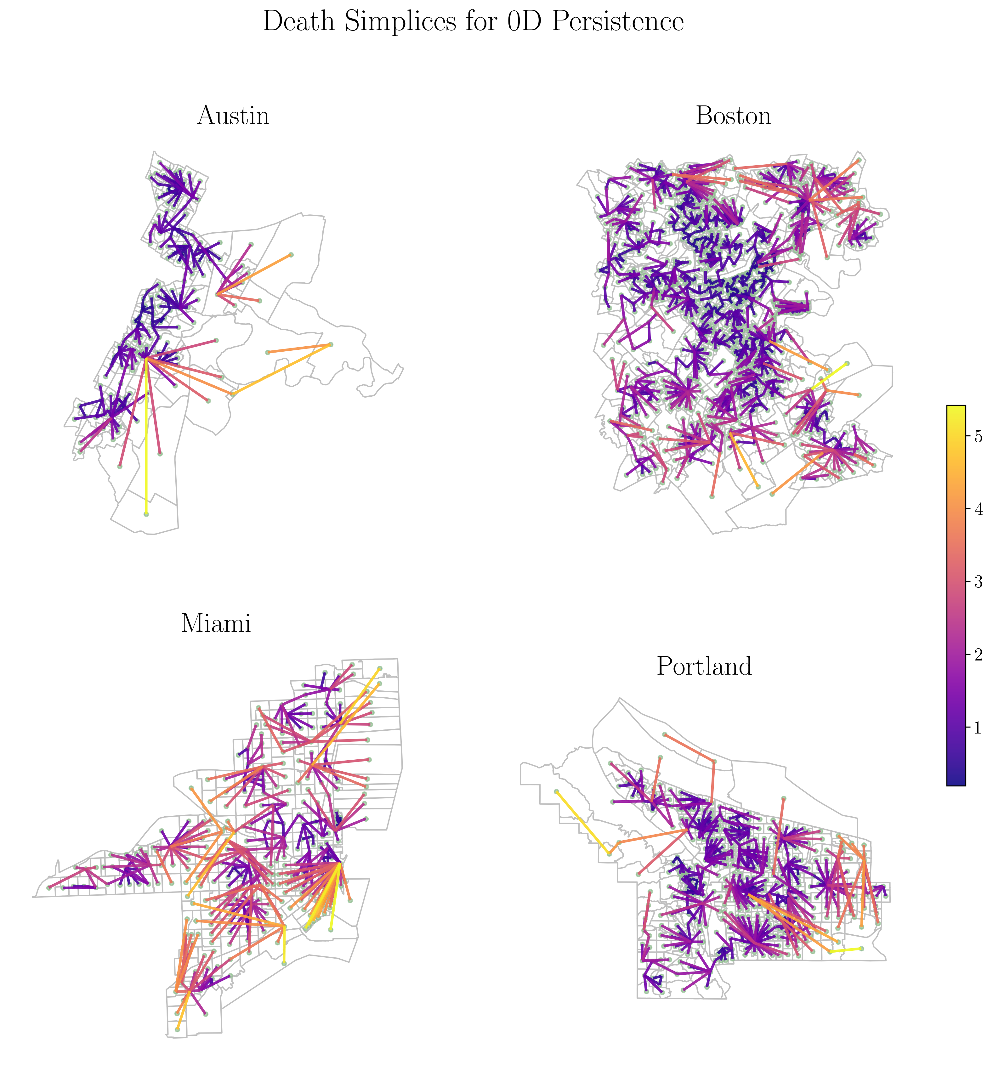
Figure 5: Map of death values for the 0-dimensional homology classes. Largest death values are represented in yellow. Maps are not to scale.

We identify the components (landmarks) that correspond to the persistence points with the five largest death times for each city. These centroids are marked with stars in Figure 6 colored based on the death time. Our topological approach identifies locations that are mostly on the edge of the city despite us adding cooling centers outside the city limits. Figure 6 also shows the census tracts with the five highest HVI scores in each city. Considering these vulnerable areas, we can suggest optimal locations for the development of future cooling centers to better serve those at risk. It can be observed that these suggested locations are frequently in areas that currently lack cooling centers. The suggestion of additional cooling centers on the eastern edge of central Austin (census tract 22.07), for example, may prove beneficial considering it has nearly 10,000 residents of whom 1,100 are of a vulnerable age to heat related mortality. Similarly, additional cooling centers in the south-east tip of Portland could cover those residents living in census tracts of high HVI scores, as seen in Figure 3.

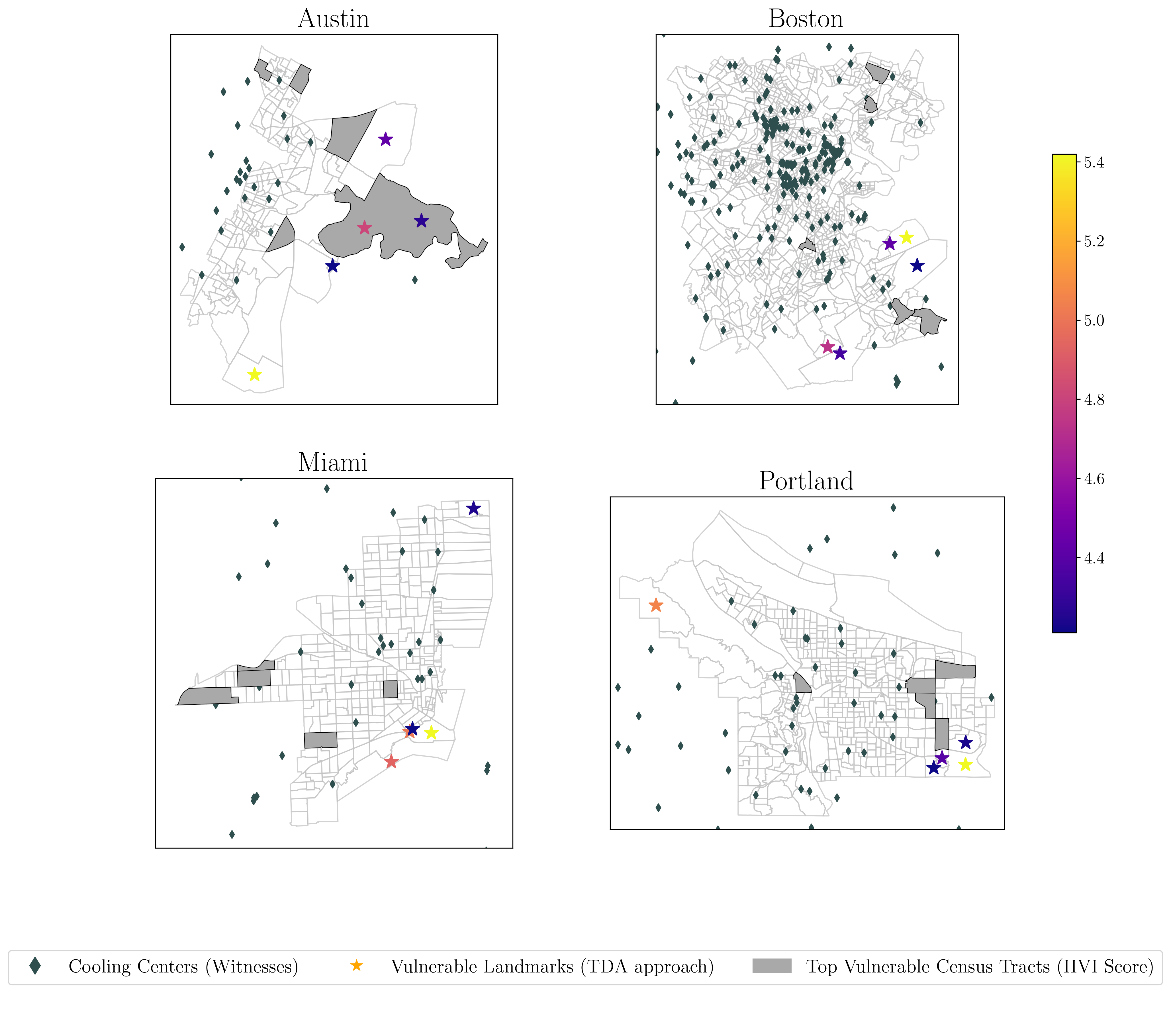
Figure 6: These maps include the distribution of cooling centers, the locations considered to have the highest vulnerability according to our TDA approach due their large death times (stars), and the top five census tracts with the largest HVI scores (grey regions). Our approach provides a complimentary set of data points to those uncovered by the HVI map.

Figure 7 maps the death simplices the 1D homology group for our four geographic locations. Death simplices with higher death value can be interpreted as a “hole” in coverage. For instance, high death values can be observed at the south-west edge of Boston and can be viewed as a high risk neighborhood during an extreme heat event.

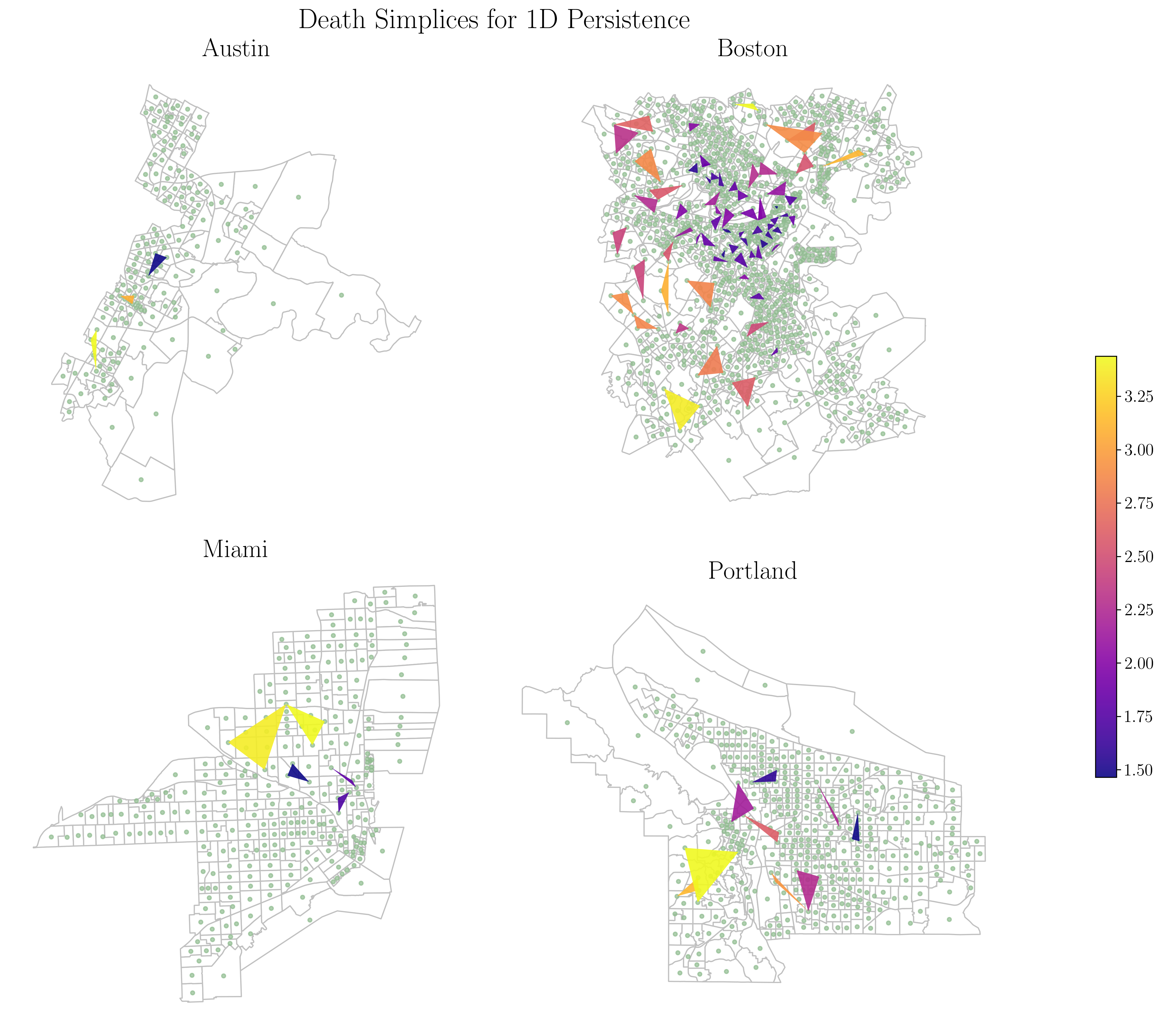
Figure 7: Map of death values for the 1-dimensional homology classes. Largest death values are represented in yellow. Maps are not to scale.

Figure 8 summarizes the 0D and 1D death values for the four locations of interest. While the differences in death times are not statistically significant, Austin has many more outliers with high death time than any other city, possibly indicating greater risk.

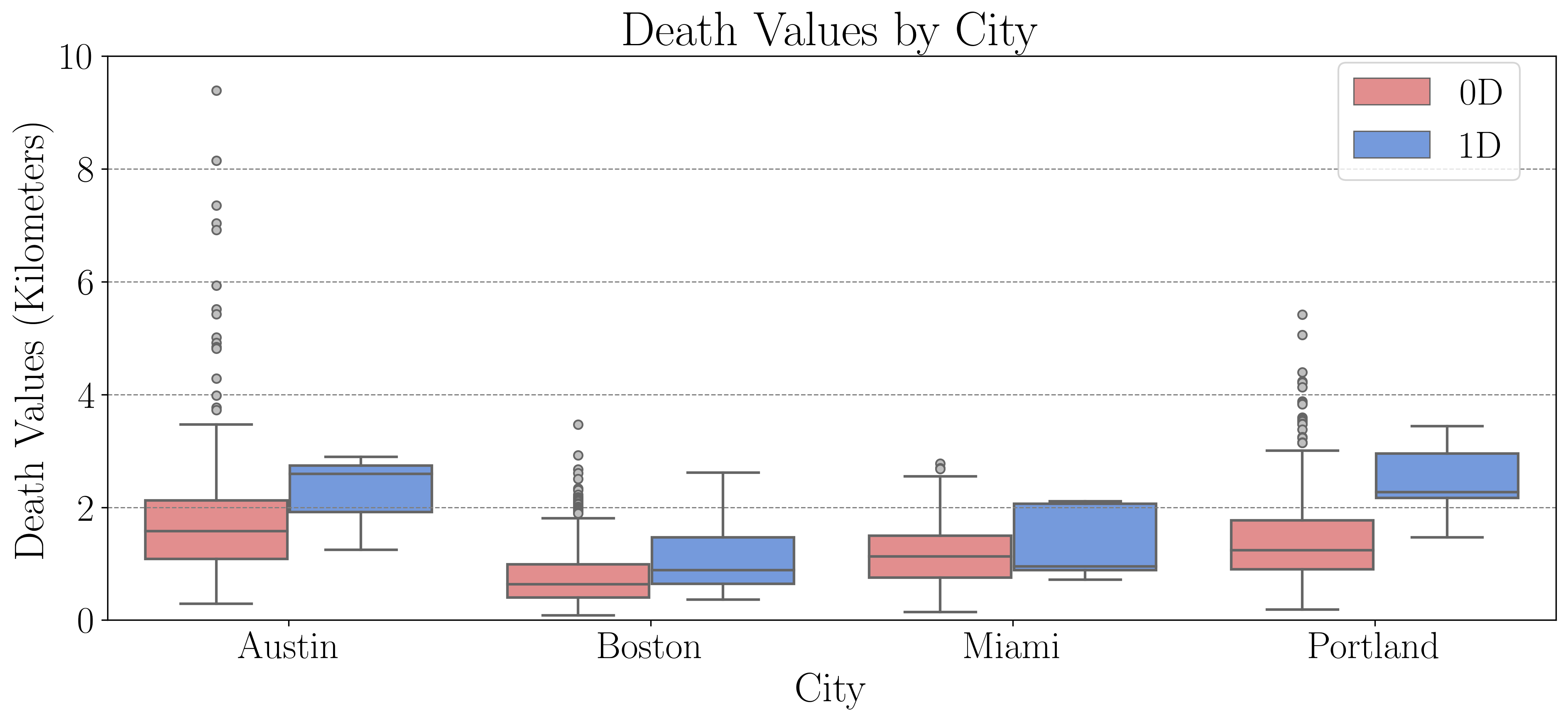
Figure 8: This box plot illustrates the death values of the 0D and 1D homology classes for each of the four geographic locations of interest.

5 Conclusion and Discussion

In this paper, we use persistent homology to determine which locations are most in need of cooling centers to reduce mortality risk. Our methodology presents some advantages over traditional approaches for analyzing cooling center coverage. Our TDA approach only requires the current distribution of cooling centers and the centroids of subdivisions (e.g. census tracts or census blocks) within a given city. Demographic data, which can be difficult to collect, is not needed. Although TDA is not a replacement to standard techniques such as an HVI map, it can identify a complementary set of high risk locations which could further inform policymakers of the ideal placement of additional cooling centers. Additionally, our approach does not treat each block as an isolated “island.” Instead, it provides a holistic evaluation of the spatial distribution of cooling centers and considers neighboring cities, adjacent blocks, and the proximity of those blocks to cooling centers.

Further, our methodology is adaptable and can be used to study access to other resources across various geographic scales other than at the census block level. We address potential future topics of study at various geographic scales in Section 5.2.

5.1 Limitations

Our methodology relies on a dataset of cooling center locations using OpenStreetMap (OSM), details of its creation are presented in Appendix A.2. However, it is important to recognize that our analysis is dependent on the quality of OSM data. For instance, the map itself may have incomplete data about a city’s current distributions of cooling centers, which could impact our results. In addition, our methodology does not account for a cooling center’s hours of operation nor capacity.

Similarly, we are limited by the completeness of the demographic data. For instance, we restricted our attention to central Austin, TX and central Boston, MA because the U.S. Urban Heat Island Mapping Campaign only included data in that region. In addition, ideally we would have demographic data at the census block level rather than the census tract level. Moreover, some census tract scores may be lower or higher in reality due to missing data. For instance, the data for census tract 9812.02 in Boston, MA showed no residents were less than 5 or over 65, which is attributed to missing data.

Lastly, it is important to address the topographical features that may limit our analysis. For one, census blocks can be different sizes within a given city. This is a problem, for example, because a centroid in a large census block may appear to be isolated spatially in our analysis and, therefore, not connect to other centroids until later in the filtration. This census block could be labelled as not being well covered, when in fact it is. Ideally, a census block’s centroid would be a good geographical approximation for any neighborhood within the census. In addition, our analysis does not account for bodies of water. For example, some unpopulated islands off the coast of Boston are included within census block boundaries without regards to the ocean.

5.2 Future Work

Future work includes adapting additional techniques used by Hickok et al. [19], such as measuring distance in travel time and incorporating several modes of transportation. Google maps has a fee for each distance calculated, so using travel time or different modes of transportation was infeasible in this case. The geodesic distance has a lower computational and monetary cost.

In the future, we would like to conduct a larger scale investigation about additional cities. We chose four different cities to test our method, however there are many other cities included in the US Urban Heat Island Mapping Campaign. Our methodology could be used in many other applications as well; for example, studying the coverage of resources such as food banks or healthy food options. On a smaller scale, one could consider the locations of automated external defibrillators (AEDs) or fire extinguishers within a large building, such as a school. A resource that will be important over the coming decades is electric vehicle charging stations. For this application, a larger statewide or nationwide scale would be useful to determine areas where the addition of a charging station would facilitate the use of electric vehicles in the area.

Appendix A Data Collection

Below describes the data sources along with any pre-processing steps applied to them. A.1 describes the landmark (census block centroids) data and A.1 describes the witness (cooling center) data. Figure 9 plots the full dataset of landmarks and witnesses.

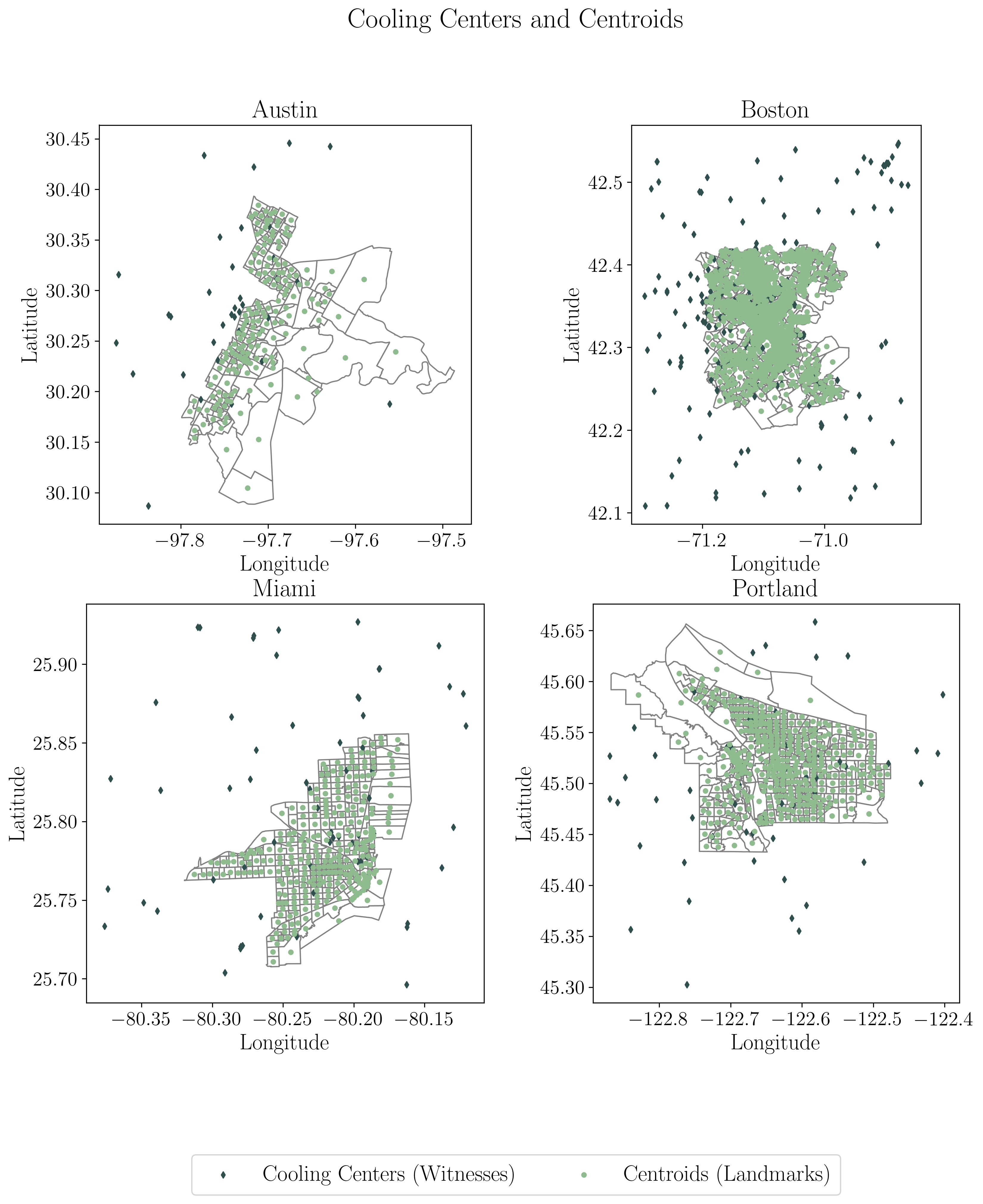
Figure 9: Final dataset of census tract centroids (landmarks) and cooling centers (witnesses) for each of the four locations, colored in light green and dark green, respectively.

A.1 Landmark Data Collection and Processing

The Shapefiles for mapping the census blocks were retrieved from Data.gov [33]. The following datasets were downloaded in July 2024:

1. TIGER/Line Shapefile, 2017, state, Massachusetts, Current Block Group State-based

2. TIGER/Line Shapefile, 2017, state, Florida, Current Block Group State-based

3. TIGER/Line Shapefile, 2017, state, Oregon, Current Block Group State-based

4. TIGER/Line Shapefile, 2017, state, Texas, Current Block Group State-based

The dataset of census block centroids were created by using the .centroid attribute of the Shapely library in Python for each of the .json files and plotted in Figure 9 in light green.

A.2 Witness Data Collection and Processing

We scan OpenStreetMap (OSM) [28] to collect the latitude and longitude coordinates of cooling centers. In order for our methodology to accurately assess the coverage of cooling centers near the boundary of the city, we buffer our search area. A buffer is necessary because a census block on the edge of the city is not restricted to only visiting cooling centers within its city. In reality, residents of that census block could travel to nearby cooling centers of neighboring cities. To create the buffer, we find the longest distance between any two census tract centroids within the city and divide that distance by 2. We use this distance as a reference to buffer the city.

We use a function within the OSMnx package, geometries_from_bbox(), to create the bounding box for our search area. The furthest southwest and northeast coordinate for the bounding box is summarized in Table 1. We search for features with the following tags: “library,” “community center,” “senior,” and “recreation center.” These tags were selected based on the definition of a cooling center presented in [24]. The dataset of cooling centers used in this study can be seen in Figure 9 in dark green.

Table 1: Furthest Southwest and Northeast coordinates used to search OpenStreetMap for cooling center tags.

City	Southwest Coordinate	Northeast Coordinate
Austin, TX	(-97.90787741442931, 30.033924160573395)	(-97.55280269603111, 30.487698664291752)
Boston, MA	(-71.29861054113876, 42.10774101580344)	(-70.85728173592592, 42.547921903453464)
Miami, FL	(-80.38082496276087, 25.68912671238342)	(-80.09556728681095, 25.9273454531309)
Portland, OR	(-122.8805563576074, 45.28572461680384)	(-122.35668691377035, 45.69996159808512)

A.3 Heat Vulnerability Index Data Collection and Processing

The following Shapefiles were downloaded in Feb 2024 to create the HVI score maps:

1. TIGER/Line Shapefile, Current, State, Massachusetts, Census Blocks

2. TIGER/Line Shapefile, 2021, State, Texas, Census Blocks

3. TIGER/Line Shapefile, 2021, State, Oregon, Census Blocks

4. TIGER/Line Shapefile, 2021, State, Florida, Census Blocks

Data on the typical afternoon temperature, the percentage of the area covered in tree canopy, number of individuals who are under 5, and number of individuals who are older than 65 was retrieved from the National Integrated Heat Health Information System (NIHHIS). The dataset was created as part of the National Oceanic and Atmospheric Administration’s (NOAA’s) “U.S. Urban Heat Island Mapping Campaign.” Data on the area not covered in tree canopy was found by subtracting the data on the percent of area covered in tree canopy in a given census tract from 100. We verified the independence of these four variables using variance inflation factor (VIF). Those results are presented in Table 2. For further information on the data variables and the data’s geographical scope refer to [26].

Table 2: Variance inflation factor (VIF) results to check for multicollinearity in the four cities of interst. Note: a VIF of 1 indicates no multicollinearity. VIFs between 1 and 5 are considered to have negligible to minimal multicollinearity.

Variable	Austin VIF	Boston VIF	Miami VIF	Portland VIF
Typical PM temp.	1.1452	2.5749	1.2388	4.9190
Tree canopy %	1.0786	2.6938	1.0098	4.8477
Population age $<$ 5	1.2158	1.4188	1.2230	1.3257
Population age $>$ 65	1.2612	1.6367	1.3503	1.3527

References

- [1] Z. Alexander, E. Bradley, J. D. Meiss, and N. F. Sanderson, Simplicial multivalued maps and the witness complex for dynamical analysis of time series, SIAM Journal on Applied Dynamical Systems, 14 (2015), p. 1278–1307, https://doi.org/10.1137/140971415.
- [2] R. L. Bliss, J. N. Katz, E. A. Wright, and E. Losina, Estimating proximity to care, Medical Care, 50 (2012), p. 99–106, https://doi.org/10.1097/mlr.0b013e31822944d1.
- [3] A. Bouchama, M. Dehbi, G. Mohamed, F. Matthies, M. Shoukri, and B. Menne, Prognostic Factors in Heat Wave–Related Deaths: A Meta-analysis, Archives of Internal Medicine, 167 (2007), pp. 2170–2176, https://doi.org/10.1001/archinte.167.20.ira70009, https://doi.org/10.1001/archinte.167.20.ira70009, https://arxiv.org/abs/https://jamanetwork.com/journals/jamainternalmedicine/articlepdf/413470/ira70009_2170_2176.pdf.
- [4] K. Bradford, L. Abrahams, M. Hegglin, and K. Klima, A Heat Vulnerability Index and Adaptation Solutions for Pittsburgh, Pennsylvania, Environmental Science & Technology, 49 (2015), pp. 11303–11311, https://doi.org/10.1021/acs.est.5b03127, https://doi.org/10.1021/acs.est.5b03127. Publisher: American Chemical Society.
- [5] M. Christenson, S. D. Geiger, J. Phillips, B. Anderson, G. Losurdo, and H. A. Anderson, Heat vulnerability index mapping for milwaukee and wisconsin, Journal of Public Health Management and Practice, 23 (2017), pp. pp. 396–403, https://www.jstor.org/stable/48517290 (accessed 2024-05-28).
- [6] K. C. Conlon, E. Mallen, C. J. Gronlund, V. J. Berrocal, L. Larsen, and M. S. O’Neill, Mapping human vulnerability to extreme heat: A critical assessment of heat vulnerability indices created using principal components analysis, Environmental Health Perspectives, 128 (2020), p. 097001.
- [7] P. Corcoran and C. B. Jones, Topological data analysis for geographical information science using persistent homology, International Journal of Geographical Information Science, (2023), p. 1–34, https://doi.org/10.1080/13658816.2022.2155654.
- [8] S. L. Cutter, B. J. Boruff, and W. L. Shirley, Social vulnerability to environmental hazards, Social Science Quarterly, 84 (2003), pp. 242–261, https://doi.org/https://doi.org/10.1111/1540-6237.8402002, https://onlinelibrary.wiley.com/doi/abs/10.1111/1540-6237.8402002, https://arxiv.org/abs/https://onlinelibrary.wiley.com/doi/pdf/10.1111/1540-6237.8402002.
- [9] T. K. Dey and Y. Wang, Computational Topology for Data Analysis, Cambridge University Press, 1 ed., Feb. 2022, https://doi.org/10.1017/9781009099950, https://www.cambridge.org/core/product/identifier/9781009099950/type/book.
- [10] H. Edelsbrunner and J. Harer, Computational Topology, American Mathematical Society, Providence, Rhode Island, Dec 2009, https://doi.org/10.1090/mbk/069, http://www.ams.org/mbk/069.
- [11] Climate Change Indicators: Heat-Related Deaths. https://www.epa.gov/climate-indicators/climate-change-indicators-heat-related-deaths, 2023. Accessed: 2023-08-24.
- [12] M. Feng and M. A. Porter, Spatial applications of topological data analysis: Cities, snowflakes, random structures, and spiders spinning under the influence, Phys. Rev. Res., 2 (2020), p. 033426, https://doi.org/10.1103/PhysRevResearch.2.033426, https://link.aps.org/doi/10.1103/PhysRevResearch.2.033426.
- [13] M. Feng and M. A. Porter, Persistent homology of geospatial data: A case study with voting, SIAM Review, 63 (2021), p. 67–99, https://doi.org/10.1137/19M1241519.
- [14] K. A. H. Francis P. Boscoe and M. S. Zdeb, A nationwide comparison of driving distance versus straight-line distance to hospitals, The Professional Geographer, 64 (2012), pp. 188–196, https://doi.org/10.1080/00330124.2011.583586, https://doi.org/10.1080/00330124.2011.583586, https://arxiv.org/abs/https://doi.org/10.1080/00330124.2011.583586.
- [15] A. M. Fraser, M. V. Chester, and D. Eisenman, Strategic locating of refuges for extreme heat events (or heat waves), Urban Climate, 25 (2018), pp. 109–119, https://doi.org/https://doi.org/10.1016/j.uclim.2018.04.009, https://www.sciencedirect.com/science/article/pii/S221209551830124X.
- [16] G. Gero, La county climate vulnerability assessment, 2021. Accessed: 2023-11-08.
- [17] S. Gillies, C. van der Wel, J. V. den Bossche, M. W. Taves, J. Arnott, and B. C. Ward, Shapely, 2024, https://doi.org/10.5281/zenodo.12737127, https://github.com/shapely/shapely.
- [18] A. A. Hagberg, D. A. Schult, and P. J. Swart, Exploring network structure, dynamics, and function using networkx, in Proceedings of the 7th Python in Science Conference, G. Varoquaux, T. Vaught, and J. Millman, eds., Pasadena, CA USA, 2008, pp. 11 – 15.
- [19] A. Hickok, B. Jarman, M. Johnson, J. Luo, and M. A. Porter, Persistent homology for resource coverage: A case study of access to polling sites, SIAM Review, 66 (2024), p. 481–500, https://doi.org/10.1137/22M150410X.
- [20] A. Hickok, D. Needell, and M. A. Porter, Analysis of spatial and spatiotemporal anomalies using persistent homology: Case studies with covid-19 data, SIAM Journal on Mathematics of Data Science, 4 (2022), pp. 1116–1144.
- [21] B. Jalalzadeh Fard, R. Mahmood, M. Hayes, C. Rowe, A. M. Abadi, M. Shulski, S. Medcalf, R. Lookadoo, and J. E. Bell, Mapping heat vulnerability index based on different urbanization levels in nebraska, usa, GeoHealth, 5 (2021), p. e2021GH000478.
- [22] S. G. Jones, A. J. Ashby, S. R. Momin, and A. Naidoo, Spatial implications associated with using euclidean distance measurements and geographic centroid imputation in health care research, Health Services Research, 45 (2010), pp. 316–327.
- [23] K. Jordahl, J. V. den Bossche, M. Fleischmann, J. Wasserman, J. McBride, J. Gerard, J. Tratner, M. Perry, A. G. Badaracco, C. Farmer, G. A. Hjelle, A. D. Snow, M. Cochran, S. Gillies, L. Culbertson, M. Bartos, N. Eubank, maxalbert, A. Bilogur, S. Rey, C. Ren, D. Arribas-Bel, L. Wasser, L. J. Wolf, M. Journois, J. Wilson, A. Greenhall, C. Holdgraf, Filipe, and F. Leblanc, geopandas/geopandas: v0.8.1, July 2020, https://doi.org/10.5281/zenodo.3946761, https://doi.org/10.5281/zenodo.3946761.
- [24] K. Kim, J. Jung, C. Schollaert, and J. T. Spector, A comparative assessment of cooling center preparedness across twenty-five u.s. cities, International Journal of Environmental Research and Public Health, 18 (2021), https://doi.org/10.3390/ijerph18094801, https://www.mdpi.com/1660-4601/18/9/4801.
- [25] G. A. Meehl and C. Tebaldi, More intense, more frequent, and longer lasting heat waves in the 21st century, Science, 305 (2004), pp. 994–997, https://doi.org/10.1126/science.1098704, https://www.science.org/doi/abs/10.1126/science.1098704, https://arxiv.org/abs/https://www.science.org/doi/pdf/10.1126/science.1098704.
- [26] U.S. Urban Heat Island Mapping Campaign. https://www.heat.gov/datasets/esri::u-s-urban-heat-island-mapping-campaign/about, 2021. [Downloaded 02-26-2024].
- [27] S. G. Nayak, S. Shrestha, S. C. Sheridan, W.-H. Hsu, N. A. Muscatiello, C. I. Pantea, Z. Ross, P. L. Kinney, M. Zdeb, S.-A. A. Hwang, and S. Lin, Accessibility of cooling centers to heat-vulnerable populations in new york state, Journal of Transport & Health, 14 (2019), p. 100563, https://doi.org/https://doi.org/10.1016/j.jth.2019.05.002, https://www.sciencedirect.com/science/article/pii/S2214140519300787.
- [28] OpenStreetMap contributors, OpenStreetMap, 2021, https://www.openstreetmap.org. Version 1.2.2 (accessed 10–11 August 2023).
- [29] D. W. Pierce, J. F. Kalansky, D. R. Cayan, et al., Climate, drought, and sea level rise scenarios for california’s fourth climate change assessment, California Energy Commission and California Natural Resources Agency, (2018).
- [30] T. G. Project, GUDHI User and Reference Manual, GUDHI Editorial Board, 3.9.0 ed., 2023, https://gudhi.inria.fr/doc/3.9.0/.
- [31] N. F. Sanderson, Topological data analyses of time series using witness complexes, PhD thesis, University of Colorado at Boulder, 2018.
- [32] V. d. Silva and G. Carlsson, Topological estimation using witness complexes , in SPBG’04 Symposium on Point - Based Graphics 2004, M. Gross, H. Pfister, M. Alexa, and S. Rusinkiewicz, eds., The Eurographics Association, 2004, https://doi.org//10.2312/SPBG/SPBG04/157-166.
- [33] U.S. Census Bureau Data Catalog. https://catalog.data.gov/organization/census-gov, 2019. [Downloaded 02-28-2023].
- [34] L. Yang, F. Qian, D.-X. Song, and K.-J. Zheng, Research on urban heat-island effect, Procedia Engineering, 169 (2016), pp. 11–18.