Fast Symbolic Integer-Linear Spectra

Abstract

Here we contribute a fast symbolic eigenvalue solver for matrices whose eigenvalues are $\mathbb{Z}$-linear combinations of their entries, alongside efficient general and stochastic $M^{X}$ generators. Users can interact with a few degrees of freedom to create linear operators, making high-dimensional symbolic analysis feasible for when numerical analyses are insufficient.

Introduction

$\mathbb{Z}$-linear eigenvalue matrices are a class of matrices which have monomial entries, and eigenvalues expressed as sums of integer multiples of their entries. Kenyon[4] and colleagues explore a subset of such matrices[9], and describe a construction below:

• Select a finite strict partial order $X$ (fig. 1)

• Determine size-n permutations (linear extensions) $\phi$ which satisfy $X$

• Create a matrix whose (i,j) entries are $\phi_{j}\phi_{i}^{-1}(id)$

• Apply the ascent-descent function $\epsilon$ on each entry (for example, $132\rightarrow 10$)

$(2<3,2<1)\rightarrow\phi=\{123,312\}$

$$\pNiceMatrix[first-col,first-row]&213312\\ 213123132\\ 231132123\rightarrow\pNiceMatrix 11&10\\ 1011\rightarrow\pNiceMatrix a_{1}&a_{2}\\ a_{2}a_{1}$$

Figure 1: A partial order and its corresponding one-line permutations. Entries of $M^{X}$ are row-inverses composed with column permutations, reduced to $01$-strings by $\epsilon$.

Matrix Generation

Users can generate arbitrary $M^{X}$ with partial order inputs, owing to the script’s dynamic programming approach which generates legal permutations from ground-up instead of filtering from the set of possible permutations.

Furthermore, a subset of partial orders always yield stochastic matrices with predictable properties. In order to guarantee stochasticity we restrict to partial orders which are fixed disjoint blocks of local transpositions, and directly take products on the possible binary sequences rather than from permutations themselves to assign monomial entries, described below:

• Select a partial order $X$ (determined by disjoint block lengths)

• Generate the corresponding $\epsilon$-filtration of possible $\pm$ sequences ($<2^{n-1}$)

• Create a matrix whose $(i,j)$ entries are $\epsilon_{\phi_{i}\phi_{j}}$ computed directly from the filtration

Rather than a partial order, users specify a dimension $n$ and factors because there could be multiple factorizations for a given $n$. Factors must be Fibonacci because they indirectly specify the length of local swap chains added to the matrix’s partial order, and such $k$-length chains yield $a_{k}=a_{k-1}+a_{k-2}$ permutations (fig. 2). Users specify the dimension $n$ with a Fibonacci-factorization of $n$ in order to specify the contribution of each local block to the total dimension. For example $\text{dfac}=\begin{bmatrix}2&13\end{bmatrix}\rightarrow n=26$. Note that if $n$ cannot be factored as such you cannot select that value.

Figure 2: Two disjoint local transposition chains where $n=16$ and $\text{fac}=\{8,2\}$. Chain lengths of length $k$ generate $fib(k)$ permutations, and matrix dimension $n$ is a product of the number of permutations each chain produces.

Partial orders are closed under concatenation of local chains, so while this construction is a strict subset, it guarantees the property holds. $M^{X}$ with disjoint block structur guarantees $\mathbb{Z}$-linear eigenvalues and provides users with a simple and well-leveraged interface, while pre-computing the direct filtration increases speed & scalability.

Figure 3: Projective barycentric coordinate for a conservative $n=3$ system where $a+b+c=1$. Allows negative masses and extension to infinity (points marked with $\pm$ are $\pm\infty$ in a given variable for $abc$).

Such matrices are desirable for Markov-type systems which are non-dissipative but not necessarily reversible (fig. 3). Furthermore they can be created faster than general matrices and instead of dealing with the complex relationships between the partial order and its corresponding matrix, users provide a small number of degrees of freedom in a highly flexible subset of $M^{X}$.

We suggest the class of matrices whose eigenvalues can be computed using $\mathbb{Z}$-linear matrix computations as a subroutine is nascent and worth exploring. For example, fractional-graph transforms[11] yield $\mathbb{R}$-linear matrices from stochastic $M^{X}$ with doubly-stochastic $D$, whose rows (columns) are permutations $\phi$ of some $x\;\;(\sum x_{i}=1,\;\;x_{i}\in\mathbb{R})$.

Theorem 1 ($\mathbb{R}$-linearity).

Given $A=Q\Lambda_{A}Q^{-1},\;x=\begin{bmatrix}x_{1}&x_{2}&\ldots&x_{n}\end{bmatrix}$:

$$D=\begin{bmatrix}\rule[2.15277pt]{10.76385pt}{0.5pt}&\phi_{1}(x)&\rule[2.15277pt]{10.76385pt}{0.5pt}\\ \rule[2.15277pt]{10.76385pt}{0.5pt}&\phi_{2}(x)&\rule[2.15277pt]{10.76385pt}{0.5pt}\\ &\vdots&\\ \rule[2.15277pt]{10.76385pt}{0.5pt}&\phi_{n}(x)&\rule[2.15277pt]{10.76385pt}{0.5pt}\end{bmatrix}=\begin{bmatrix}|&|&&|\\ \phi_{1}(x)&\phi_{2}(x)&\ldots&\phi_{n}(x)\\ |&|&&|\end{bmatrix},\;D_{ij}=D_{ji},\;D\mathbf{1}=\mathbf{1}$$

$$\Lambda_{DAD^{T}}=D\Lambda_{A}D^{T}$$

for any such $D$.

Eigenvalue Computation

Time complexity of numerical eigenvalue calculation with QR is $O(n^{3})$ for dense matrices[12]. Big O time complexity for symbolic eigenvalue calculation is extremely high and far less clear, suffering from complexities of symbolic root finding and intermediate expression swell [6]. Our algorithm achieves similar time complexity to the numerical case made possible by casting the symbolic problem into a numerical form.

Symbols used in elements of the matrix are encoded as unique power terms, resulting in pseudo-symbolic numerical values for each element, reminiscent of Gödel numbering, but here expressly with the purpose of computational performance. By exploiting the structure of $\mathbb{Z}$-linearity, we ensure power terms do not mix

The time complexity is $O(n^{3}\cdot b\log b)$ for dense matrices of dimension $n$ with $b$ bits of precision, where $b$ is in in the worst case a constant multiple of $n$. As a parallel algorithm however, the parallel span is only $O(n^{3})$, since the impact of precision becomes constant as the number of processors $p\rightarrow n$ in the batched computation.

Each batch requires digit precision only equal to its batch size and can be run in parallel, masking out all but the smaller set of batched symbols in the input matrix before running the numeric solver. The respective partial eigenvalues are summed together after to achieve the final result.

We created implementations of the $\mathbb{Z}$LE eigenvalue algorithm in Python, Mathematica, and C++ to allow a range of accessibility and performance.

Runtime Comparison

C++ (s)
n $\mu$ $\sigma$ 13 0.010 0.047e-2 21 0.027 0.047e-2 34 0.091 0.082e-2 55 0.319 0.002 89 1.723 0.057 144 6.381 0.246 233 43.810 0.480 377 158.374 1.590 610 690.556 25.591 987 3007.097 108.985

Figure 4: Symbolic eigenvalue computation times for: Mathematica’s built-in symbolic solver, and our 3 $\mathbb{Z}LE$ libraries (Python, Mathematica, and C++).

Applications

We can treat stochastic $\mathbb{Z}$-linear eigenvalue matrices as generator matrices by subtracting their row-sums along the diagonal, allowing us to adopt a multidimensional Markov chain formalism[3] often used in stochastic automata networks (SAN).

$$Q=Q_{0}+Q_{D},\;\;Q_{0}=\sum_{k=1}^{K}\bigotimes_{h=1}^{H}Q_{k}^{(h)},\;\;Q_{D}=-diag{(Q_{0}e)}$$

$$Q_{local}=\sum_{k=1}^{H}\bigotimes_{h=1}^{H}Q_{k}^{(h)},\;Q_{synchronized}=\sum_{k=H+1}^{K}\bigotimes_{h=1}^{H}Q_{k}^{(h)}$$

Figure 5: MDMC. $e$: the $\mathbf{1}$s vector, $H$: $\#$ factors in each term, $K$: $\#$ terms. Subsystems $1,\ldots,H$ model local transitions, $H+1,\ldots,K$ model synchronized transitions

Such models are relevant because of the properties of tensor products and sums. For eigenvalues $\lambda$ and $\mu$ of $A$ and $B$ and their eigenvectors $x$ and $y$, $A\otimes B$ contains eigenvalues $\lambda\mu$ paired with eigenvectors $x\otimes y$. Eigenvalues of $A\oplus B$ come in the form $\lambda+\mu$ with eigenvectors $x\otimes y$. Since the probability transition matrix $P$ is the matrix exponential of the generator matrix $G$, $P=e^{Q}Q(0)$, we can see how the term ’local’ comes from the capacity to factor the exponential and isolate the first $H$ terms, while synchronized transitions couple together due to the eigenvalues being products rather than sums. By treating $M^{X}$ matrices as building blocks in the MDMC formalism we can easily trace spectral contributions from each factor.

One simple way to get generators from these matrices is to add $Q_{D}=-diag(Q_{0}e)$. We can build multidimensional models with local and synchronous transitions in any fashion and make sure rows sum to 0. Consider two matrices $A$ and $B$ -

$A=\bNiceMatrix[first-row,last-row,first-col,last-col]&_{1}{}_{2}{}_{3}\\ _{1}abc\\ _{2}bac\\ _{3}cba\\$ $\qquad\;\;B=\bNiceMatrix[first-row,last-row,first-col,last-col]&_{4}{}_{5}\\ _{4}de\\ _{5}ed\\$

$$a+b+c+d+e=k$$

$$Q_{A\oplus B}=\bNiceArray{ccccccc}[small,first-col,first-row]&_{(1,4)}{}_{(1,5)}{}_{(2,4)}{}_{(2,5)}{}_{(3,4)}{}_{(3,5)}\\ _{(1,4)}a+d-keb0c0\\ _{(1,5}ea+d-k0b0c\\ _{(2,4)}b0a+d-kec0\\ _{(2,5)}0bea+d-k0c\\ _{(3,4)}c0b0a+d-ke\\ _{(3,5)}0c0bea+d-k\\$$

$$\sigma_{Q_{A\oplus B}}=-k+\text{map}((\lambda,\mu)\rightarrow\lambda+\mu,\;\sigma_{A}\bigtimes\sigma_{B})$$

$$(a+b+c)(d+e)=k$$

$$Q_{A\otimes B}=\bNiceArray{ccccccc}[small,first-col,first-row]&_{(1,4)}{}_{(1,5)}{}_{(2,4)}{}_{(2,5)}{}_{(3,4)}{}_{(3,5)}\\ _{(1,4)}ad-kaebdbecdce\\ _{(1,5)}aead-kbebdcecd\\ _{(2,4)}bdbead-kaecdce\\ _{(2,5)}bebdaead-kcecd\\ _{(3,4)}cdcebdbead-kae\\ _{(3,5)}cecdbebdaead-k\\$$

$$\sigma_{Q_{A\otimes B}}=-k+\text{map}((\lambda,\mu)\rightarrow\lambda\cdot\mu,\;\sigma_{A}\bigtimes\sigma_{B})$$

Figure 6: Local $A\oplus B$ (above) and synchronous $A\otimes B$ transitions (below). Eigenvalues $\sigma$ are sums or products of those from $A$ and $B$. State diagrams are provided to delineate between these two types of transitions.

The SAN accessible from elementary $M^{X}$ matrix units provides a rich baseline of multidimensional models. Not only are they expressive, but also have many memory- and time-efficient representations.

$$Q_{0}=\bigoplus_{i=1}^{H}Q_{i}^{(i)}$$

$$e^{Qt}Q(0)=e^{Q}=e^{\bigoplus_{i=1}^{H}Q_{i}^{(i)}+Q_{D}}=e^{\bigoplus_{i=1}^{H}Q_{i}^{(i)}}e^{Q_{D}}=e^{Q_{D}}\bigotimes_{h=1}^{H}e^{Q_{i}^{(i)}}=e^{Q_{D}}\bigotimes_{h=1}^{H}P_{i}^{(i)}$$

Relating $P$ and $Q$ in a local MDMC by exploiting the identity $e^{x\oplus y}=e^{x}\otimes e^{y}$[10].

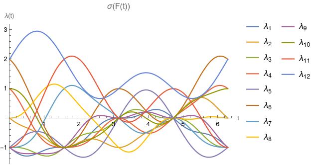
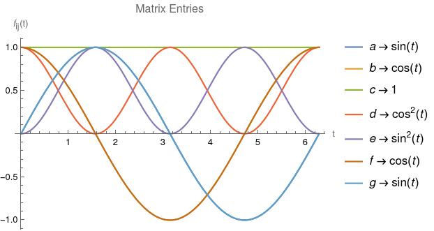
Figure 7: Given eigenvalue constraints for $F(t)$, find time-varying matrix entries $f_{ij}(t)$ ($\sigma(F(t))$ plotted with scale parameter $s=\frac{1}{2}$).

$$F(t)=s\bigoplus_{i=1}^{H}Q_{i}+(1-s)\bigotimes_{i=1}^{H}Q_{i}+Q_{D}$$

$$Q_{1}=\begin{bmatrix}a(t)&b(t)\\ b(t)&a(t)\end{bmatrix},\;Q_{2}=\begin{bmatrix}c(t)&d(t)&e(t)\\ d(t)&c(t)&e(t)\\ e(t)&d(t)&c(t)\end{bmatrix},\;Q_{3}=\begin{bmatrix}f(t)&g(t)\\ g(t)&f(t)\end{bmatrix}$$

One toy model, $F(t)$, is a $12$-dimensional convex combination of local and synchronous transitions sharing the same 3 factors $Q_{i}$ of dimensions $2,3,2$. $s\in[0,1]$ scales their proportions. Note that in general the system is underdetermined but particular solutions exist, such as those for the eigenvalues shown in fig. 7.

Conclusion

Users can generate matrices and find symbolic eigenvalues which are $\mathbb{Z}$-linear combinations of matrix entries. Eigenvalues which are products of monomials and/or have real-valued coefficients can be achieved directly from $M^{X}$ calculations through tensor products and $\mathbb{R}$-linearity (theorem 1). We hope this toolkit benefits researchers in any befitting domain, which includes but is not limited to reduced order modeling & control, conservative systems, and large-scale numeric quantum simulations.

Future Directions

A similar treatment for eigenvectors is equally important and needed. Generating a closest suitable matrix still requires expert knowledge for distance norm selection and application, so a procedural method for inferring $\mathbb{Z}$-linear matrices would be useful. We suspect that extensions of complex numbers such as quaternions could decrease runtime by storing variables in more than just one imaginary component. We look forward to progress in computing fast eigenvalues with complex algebraic structure through novel means of encrypting symbolic terms in a numeric context.

References

- Anderson et al. [1999] E. Anderson, Z. Bai, C. Bischof, S. Blackford, J. D. J. Dongarra, J. D. Croz, A. Greenbaum, S. Hammarling, A. McKenney, and D. Sorensen. LAPACK Users’ Guide. SIAM, Philadelphia, Pennsylvania, USA, third edition, 1999.
- Blackford et al. [2002] L. S. Blackford, A. Petitet, R. Pozo, K. Remington, R. C. Whaley, J. Demmel, J. Dongarra, I. Duff, S. Hammarling, G. Henry, et al. An updated set of basic linear algebra subprograms (blas). ACM Transactions on Mathematical Software, 28(2):135–151, 2002.
- Dayar [2012] T. Dayar. Analyzing markov chains using Kronecker products: Theory and applications. Springer, 2012.
- Kenyon et al. [2024] R. Kenyon, M. Kontsevich, O. Ogievetsky, C. Pohoata, W. Sawin, and S. Shlosman. The miracle of integer eigenvalues, 2024. URL https://arxiv.org/abs/2401.05291.
- Meurer et al. [2017] A. Meurer, C. P. Smith, M. Paprocki, O. Čertík, S. B. Kirpichev, M. Rocklin, A. Kumar, S. Ivanov, J. K. Moore, S. Singh, T. Rathnayake, S. Vig, B. E. Granger, R. P. Muller, F. Bonazzi, H. Gupta, S. Vats, F. Johansson, F. Pedregosa, M. J. Curry, A. R. Terrel, v. Roučka, A. Saboo, I. Fernando, S. Kulal, R. Cimrman, and A. Scopatz. Sympy: symbolic computing in python. PeerJ Computer Science, 3:e103, Jan. 2017. ISSN 2376-5992. doi: 10.7717/peerj-cs.103. URL https://doi.org/10.7717/peerj-cs.103.
- Moses [1971] J. Moses. Algebraic simplification: A guide for the perplexed, 1971.
- mpmath development team [2023] T. mpmath development team. mpmath: a Python library for arbitrary-precision floating-point arithmetic (version 1.3.0), 2023. https://mpmath.org/.
- Nakata [2022] M. Nakata. Mplapack version 2.0.1 user manual, 2022.
- Ogievetsky and Shlosman [2018] O. V. Ogievetsky and S. B. Shlosman. Plane partitions and their pedestal polynomials, May 2018.
- Plateau [1985] B. Plateau. On the stochastic structure of parallelism and synchronization models for distributed algorithms, Aug 1985.
- Scheinerman and Ullman [2013] E. R. Scheinerman and D. H. Ullman. Fractional Graph Theory: A Rational Approach to the Theory of Graphs. Dover Publications, 2013.
- Strang [2019] G. Strang. Linear Algebra and learning from data (2019). Wellesley-Cambridge Press, 2019. URL https://math.mit.edu/~gs/learningfromdata/.