Linear Convergence of Diffusion Models Under the Manifold Hypothesis

Abstract

Score-matching generative models have proven successful at sampling from complex high-dimensional data distributions. In many applications, this distribution is believed to concentrate on a much lower $d$-dimensional manifold embedded into $D$-dimensional space; this is known as the manifold hypothesis. The current best-known convergence guarantees are either linear in $D$ or polynomial (superlinear) in $d$. The latter exploits a novel integration scheme for the backward SDE. We take the best of both worlds and show that the number of steps diffusion models require in order to converge in Kullback-Leibler (KL) divergence is linear (up to logarithmic terms) in the intrinsic dimension $d$. Moreover, we show that this linear dependency is sharp.

1 Introduction

Score-matching generative models (Ho et al., 2020; Song et al., 2021) such as diffusion models have become a leading paradigm for generative modeling. They achieve state-of-the-art results in many domains including audio/image/video synthesis (Evans et al., 2024; Dhariwal and Nichol, 2021; Ho et al., 2022), molecular modeling (Watson et al., 2023), and recently text generation (Lou et al., 2024). Informally, diffusion models take samples from a distribution in $\mathbb{R}^{D}$, gradually corrupt them with Gaussian noise, and then learn to reverse this process. Once trained, a diffusion model can turn noise into new samples from the data distribution by iteratively applying the denoising procedure.

Due to the empirical success of diffusion models, there has been a push (Oko et al., 2023; Wibisono et al., 2024; Wu et al., 2024) to better understand their theoretical properties, in particular, their convergence guarantees.

An important question is to determine the iteration complexity of diffusion models. In this paper, this refers to the number of steps diffusion models require in order to converge in $\operatorname{\mathsf{KL}}$ to the original distribution regularized by a small amount of Gaussian noise. Assuming only the existence of a second moment, Benton et al. (2024) prove that the iteration complexity is at most linear (up to logarithmic factors) in $D$.

While this result is tight in the general case, many real-world distributions actually have a low-dimensional structure. The assumption that a distribution lives on a $d$-dimensional manifold is called the manifold hypothesis. This hypothesis has been supported by empirical evidence in many settings, e.g. image data, in which diffusion models are particularly successful. Therefore, the study of diffusion models under this assumption has garnered increased interest (Kadkhodaie et al., 2024; Tang and Yang, 2024; Pidstrigach, 2022).

Recently Li and Yan (2024a) have shown that there is a special discretization design guaranteeing an iteration complexity of $d^{4}$ in the intrinsic dimension $d$. The current (Azangulov et al., 2024) best-known bound scales as $d^{3}$.

Our Contribution

In this work, we improve upon these results and show that the number of steps diffusion models require to converge in KL divergence is linear (up to logarithmic terms) in the intrinsic dimension $d$. This is formalized in Theorem 3. Additionally, we prove that the linear dependency is sharp.

The proof follows the structure of Chen et al. (2023b) and Benton et al. (2024) combined with a result from Azangulov et al. (2024) providing bounds on the score function depending only on the intrinsic dimension $d$. A key insight of our proof exploits the inherent martingale structure in diffusion processes. As we show, with the right SDE discretization, the corresponding error can be represented as a sum of easy-to-control martingale increments leading to a very concise argument.

We posit that this scaling is one of the major reasons why diffusion models are able to perform so well on tasks such as synthetic image generation. While the extrinsic dimension of image datasets is very large, e.g. $\approx 1.5\cdot 10^{5}$ for ImageNet,  Pope et al. (2021) estimate that the true intrinsic dimension is much lower, e.g. around $50$ for ImageNet. Our result implies that the number of steps diffusion models need to sample scales as the latter rather than the former. This helps explain why diffusion models are able to generate crisp image samples with less than $1000$ iterations (Ho et al., 2020).

In Section 2, we give an overview of diffusion models, our assumptions and the discretization scheme that we use. We introduce our main result in Section 3 and give its proof in Section 4. We conclude in Section 5.

2 Preliminaries

2.1 Diffusion Models

Suppose we want to generate samples from a distribution $\mu$ on $\mathbb{R}^{D}$. Diffusion models solve this by first specifying a forward noising process $\{X_{t}\}_{t\in[0,T]}$ up to some time $T$. This process is defined as the evolution of data $X_{0}\sim\mu$ according to an Ornstein-Uhlenbeck (OU) SDE

$$\begin{cases}dX_{t}=-X_{t}dt+\sqrt{2}dB_{t},&t\in(0,T]\\ X_{0}\sim\mu,\end{cases}$$

where $\{B_{t}\}_{t\in[0,T]}$ is a Brownian motion on $\mathbb{R}^{D}$. Letting $c_{t}:=\exp(-t)$ and $\sigma^{2}_{t}:=1-\exp(-2t)$, we note that $X_{t}\stackrel{{\scriptstyle dist.}}{{=}}c_{t}X_{0}+\sigma_{t}Z_{D}$ where $Z_{D}\sim\mathcal{N}(0,\operatorname{\mathrm{Id}}_{D})$. We use $p_{t}$ to denote the marginal density of $X_{t}$.

The reverse process $\{Y_{t}\}_{t\in[0,T]}:=\{X_{T-t}\}_{t\in[0,T]}$, under mild assumptions Anderson (1982), satisfies

$$\begin{cases}dY_{t}=(Y_{t}+2\nabla\log p_{T-t}(Y_{t}))dt+\sqrt{2}dB_{t}^{\prime},&t\in(0,T]\\ Y_{0}\sim p_{T},\end{cases}$$ (1)

where $\{B_{t}^{\prime}\}_{t\in[0,T]}$ is another Brownian motion on $\mathbb{R}^{D}$. By generating samples $Y_{0}\sim p_{T}$ and then simulating (1) up to time $T$, we can obtain samples $Y_{T}\sim\mu$ from the data distribution. The main idea behind diffusion models is to simulate these dynamics approximately since neither $p_{T}$ nor the score function $s_{t}:=\nabla\log p_{t}$ are known.

In practice, we solve these problems by building an approximate process $\hat{Y}_{t}$. Due to the exponential convergence of the OU process to a standard normal distribution, for a sufficiently large $T$, we have that $p_{T}\approx\mathcal{N}(0,\operatorname{\mathrm{Id}}_{D})$. So, we initialize as $\hat{Y}_{0}\sim\mathcal{N}(0,\operatorname{\mathrm{Id}}_{D})$. Second, we learn a score approximation $\hat{s}_{t}\approx s_{t}$ which is used instead of the true score function. The approximation $\hat{s}_{t}$ is usually parameterized by neural networks and trained via a denoising score-matching objective.

Finally, we note that the SDE (1) cannot be simulated exactly and instead a discretization scheme must be introduced. More precisely, first, in order to ensure numerical stability, an early stopping time $\delta>0$ is chosen. Next, the interval $[0,T-\delta]$ is divided into $K$ time steps $0=t_{0}<t_{1}<\ldots<t_{K}=T-\delta$. The final discretization is given by

$$\begin{cases}\hat{Y}_{t_{k+1}}=\alpha_{k}\hat{Y}_{t_{k}}+\beta_{k}\hat{s}_{T-t_{k}}(\hat{Y}_{t_{k}})+\eta_{k}Z_{k},&0\leq k<K\\ \hat{Y}_{t_{0}}\sim\mathcal{N}\left(0,\operatorname{\mathrm{Id}}_{D}\right),\end{cases}$$ (2)

where $Z_{k}\stackrel{{\scriptstyle i.i.d.}}{{\sim}}\mathcal{N}(0,\operatorname{\mathrm{Id}}_{D})$ and $\alpha_{k},\beta_{k},\eta_{k}$ are real numbers. The discretization schedule $t_{0}<t_{1}<\ldots<t_{K}$ and coefficients $\alpha_{k},\beta_{k},\eta_{k}$ are hyper-parameters which we will specify in Section 2.3.

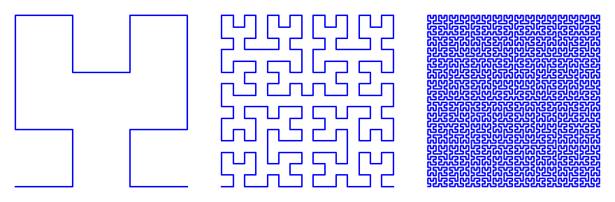
(a) Hilbert curves of orders $n=2,4,6$

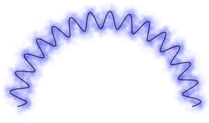
(b) Premature early stopping leads to over-smoothing of the manifold structure

2.2 Assumptions and Notation

Throughout the paper, we assume that the distribution $\mu$ satisfies the manifold hypothesis which we state more formally in the following.

Assumption A.

$\mu$ is supported on a smooth compact $d$-dimensional $\beta\geq 2$-smooth manifold $M$ embedded into $\mathbb{R}^{D}$.

We also make the following assumption for ease of presentation. The general case is handled by rescaling and shifting.

Assumption B.

We assume $\operatorname{\operatorname{diam}}M\leq 1$ and $0\in M$.

Without any restrictions on the manifold $M$, we cannot hope to obtain bounds independent of the ambient dimension $D$. As an intuitive counter-example, consider $D$-dimensional Hilbert curves $M_{n}$, see Fig. 1(a). In the limit, these curves cover the entire $D$ dimensional cube $M_{\infty}:=[0,1]^{D}$. Moreover, any measure on $M_{\infty}$ can be seen as a weak limit of measures on $M_{n}$. This makes sampling from $M_{n}$ (for large enough $n$) as hard as sampling from $M_{\infty}$, which according to (Benton et al., 2024, Appendix H) scales as at least $D$.

Therefore, we should place additional assumptions on the complexity of $\mu$ and $M$ in order to avoid such pathological cases. Informally (see details in Appendix A), the complexity of $M$ depends both on its global (volume) and local (smoothness) properties. We control its smoothness by introducing a scale $r>0$ at which $M$ is locally flat. To control the measure $\mu$, we assume that it has a density $p_{0}(dy)$ (w.r.t. the standard volume form $dy$) bounded from above and below. We assume logarithmic control over the discussed quantities.

Assumption C.

There is a constant $C>0$ such that $\operatorname{\mathrm{Vol}}M\leq e^{C}$, $r>e^{-C}$, and $e^{-C}\leq p_{0}\leq e^{C}$.

Remark 1.

Informally, on a scale larger than $r$, the manifold $M$ is not flat anymore. So, if $M$ is corrupted by noise of magnitude greater than $r$, over-smoothing may destroy the geometric structure, see Fig. 1(b). Diffusion models stopped at time $\delta$ add Gaussian noise proportional to $\sqrt{\delta}$. To capture its shape, $M$ shouldn’t be corrupted by noise of magnitude greater than $r$. So, the stopping time should be chosen to satisfy $\sqrt{\delta}\lesssim r$. Thus we should expect $\log\delta^{-1}\geq C$.

Recall that $\delta$ denotes the early stopping time, and $0=t_{0}<t_{1}<\ldots<t_{K}=T-\delta$ are the $K$ discretization time steps. Let $\gamma_{k}:=t_{k+1}-t_{k}$ be the $k$-th step size. We control the score estimation error of $\hat{s}_{t}$ as follows.

Assumption D.

The score network $\hat{s}_{t}(x)$ satisfies

$$\sum_{k=0}^{K-1}\gamma_{k}\operatorname{\mathbb{E}}\|s_{T-t_{k}}(X_{T-t_{k}})-\hat{s}_{T-t_{k}}(X_{T-t_{k}})\|^{2}\leq\varepsilon_{score}^{2}.$$

2.3 Discretization Scheme

In this section, we recall the construction of a discretization scheme that allows for a polynomial convergence in the intrinsic dimension $d$. The main goal of this paper is to show that this convergence is, in fact, linear. We follow the discretization schedule in Benton et al. (2024). Fix a positive $\kappa<1/4$ and choose a partition $0=t_{0}<t_{1}<\ldots<t_{K}=T-\delta$ such that $\gamma_{k}=t_{k+1}-t_{k}\leq\kappa\min\left(1,T-t_{k}\right)$.

Remark 2.

For example, fixing integers $L,K$, and choosing $T:=\kappa L+1$ and $\delta:=(1+\kappa)^{L-K}$, one can take the uniform partition $t_{k}=\kappa k,k<L$ of $[0,T-1]$ and the exponential partition $t_{L+m}=T-(1+\kappa)^{-m}$ of $[T-1,T-\delta]$ for $0\leq m\leq K-L$. We use this explicit schedule in what follows.

The class of discretization schemes of the form (2) contains a unique one, first found by Li and Yan (2024a), that has an iteration complexity independent of $D$. It is given by

$$\begin{cases}\hat{Y}_{t_{k+1}}=c^{-1}_{\gamma_{k}}\hat{Y}_{t_{k}}+\frac{\sigma^{2}_{\gamma_{k}}}{c_{\gamma_{k}}}\hat{s}_{T-t_{k}}(\hat{Y}_{t_{k}})+\sigma_{\gamma_{k}}\frac{\sigma_{T-t_{k+1}}}{\sigma_{T-t_{k}}}Z_{k},&Z_{k}\stackrel{{\scriptstyle i.i.d.}}{{\sim}}\mathcal{N}(0,\operatorname{\mathrm{Id}}_{D})\\ \hat{Y}_{t_{0}}\sim\mathcal{N}\left(0,\operatorname{\mathrm{Id}}_{D}\right).\end{cases}$$ (3)

Let us fix some $(t,x),(t^{\prime},x^{\prime})\in\mathbb{R}_{+}\times\mathbb{R}^{D}$. The classic exponential integrator scheme uses $\hat{s}(t^{\prime},x^{\prime})$ as an estimate of the true score $s(t,x)$. Azangulov et al. (2024) shows that, in contrast, (3) implicitly applies a first-order correction of the score. More precisely, they prove that if we introduce

$$\hat{s}_{t}(x|t^{\prime},x^{\prime}):=c^{-1}_{t^{\prime}-t}\frac{\sigma^{2}_{t^{\prime}}}{\sigma^{2}_{t}}\hat{s}(t^{\prime},x^{\prime})-\frac{x-c^{-1}_{t^{\prime}-t}x^{\prime}}{\sigma^{2}_{t}},$$ (4)

then the scheme (3) corresponds to the continuous time dynamics given by

$$\begin{cases}d\hat{Y}_{t}=\left[\hat{Y}_{t}+2\hat{s}_{T-t}(\hat{Y}_{t}|T-t_{k},\hat{Y}_{t_{k}})\right]dt+\sqrt{2}dB_{t}^{\prime},&t\in[t_{k},t_{k+1})\\ \hat{Y}_{0}\sim\mathcal{N}\left(0,\operatorname{\mathrm{Id}}_{D}\right).\end{cases}$$ (5)

This can be proven by integrating the linear SDE (5). The properties of the linear correction (4) will become apparent in the proof of our main result. See (9) and then a discussion in Remark 5. We analogously define $s_{t}(x|t^{\prime},x^{\prime})$ to be a correction of the true score obtained by substituting $s(t^{\prime},x^{\prime})$ instead of $\hat{s}(t^{\prime},x^{\prime})$ into (4).

3 Main Results

The main result of our paper is the following.

Theorem 3.

Let $\mu$ be a measure satisfying Assumptions A–C and let $\hat{s}_{t}$ be a score approximation satisfying D. Then the process $\hat{Y}_{t}$ following (3) and the discretization schedule defined in Section 2.3 satisfies

$$\operatorname{\mathsf{KL}}(\hat{Y}_{T-\delta}\|X_{\delta})\lesssim\varepsilon^{2}_{score}+De^{-2T}+\kappa+d\kappa^{2}(K-L)\left(\log\delta^{-1}+C\right),$$ (6)

where we use $\operatorname{\mathsf{KL}}(X\|Y)$ to denote the $\operatorname{\mathsf{KL}}$-divergence between the laws of $X$ and $Y$.

This bound consists of four terms: (i) $\varepsilon^{2}_{score}$ corresponding to the error in score approximation; (ii) $De^{-2T}$ corresponding to the initialization error; (iii) $\kappa$ corresponding to the discretization error for $t\in[0,T-1]$; (iv) $d\kappa^{2}(K-L)(\log\delta^{-1}+C)$ corresponding to the discretization error for $t\in[T-1,T-\delta]$. By choosing $K$ to be sufficiently large, we obtain a linear (up to logarithmic factors) in $d$ bound on the iteration complexity in the following.

Corollary 4.

Under the same assumptions as in Theorem 3, for a given $\kappa<1/4$ and tolerance $\varepsilon>0$, choosing $L\simeq\kappa^{-1}\left(\log D+\log\varepsilon^{-1}\right)$ and $K-L\simeq\kappa^{-1}\log\delta^{-1}$, diffusion models with $K$ denoising steps achieve an error bounded as

$$\operatorname{\mathsf{KL}}(\hat{Y}_{T-\delta}\|X_{\delta})\lesssim\varepsilon^{2}+\varepsilon^{2}_{score}+\frac{d(\log\delta^{-1}+\log\varepsilon^{-1}+\log D)(\log\delta^{-1}+C)\log\delta^{-1}}{K}.$$

Tightness of linear bound.

In the best case, a diffusion model learns the score function exactly. Let $\pi$ be a compactly supported distribution on $\mathbb{R}$ such that a diffusion model with a given discretization scheme and perfect score achieves an $\varepsilon$ error in $\operatorname{\mathsf{KL}}$.

Consider the product measure $\pi^{\otimes d}\otimes\left(\delta_{0}\right)^{\otimes(D-d)}$ on $\mathbb{R}^{d}\times\mathbb{R}^{D-d}$. Note that its score function is $(s_{t}(x_{1}),\ldots,s_{t}(x_{d}),-\sigma^{-2}_{t}x_{d+1},\ldots,-\sigma^{-2}_{t}x_{D})$. So, by the tensorization of $\operatorname{\mathsf{KL}}$, applying the same discretization scheme as above with the new exact score has a $d\varepsilon$ error. Therefore a linear dependence in $d$ is optimal.

4 Proof of Theorem 3

We defer the proofs of lemmas to Appendix B. The main idea of the proof of Theorem 3 is to exploit the martingale structure of $\operatorname{\mathbb{E}}[X_{0}|X_{t}]$. So, we begin by formalizing this before proceeding to the main proof. We introduce the functions $m_{t}(x):=\operatorname{\mathbb{E}}[X_{0}|X_{t}=x]$ and define a stochastic process $\{m_{t}(X_{t})\}_{t\in[0,T]}$. Note that $m_{t}(X_{t})=\operatorname{\mathbb{E}}[X_{0}|X_{t}]$. The next lemma states that this process is a martingale. lemmaReverseMartingale Define the filtration $\mathcal{F}_{t}:=\sigma(X_{s}:s\geq t)$. The process $\{m_{t}(X_{t})\}_{t\in[0,T]}$ is a martingale w.r.t. $\{\mathcal{F}_{t}\}_{t\in[0,T]}$. In particular, for $t<t^{\prime}$

$$\operatorname{\mathbb{E}}[m_{t}(X_{t})|X_{t^{\prime}}]=m_{t^{\prime}}(X_{t^{\prime}}).$$ (7)

By A, $X_{0}$ is a.s. bounded. Therefore the process $\{m_{t}(X_{t})\}_{t\in[0,T]}$ is square integrable. So, the following lemma on the orthogonality of martingale increments can be applied. lemmaMartingaleIncrements Let $\{M_{t}\}_{t\geq 0}$ be a square integrable martingale in $\mathbb{R}^{D}$ w.r.t. a filtration $\{\mathcal{F}_{t}\}_{t\geq 0}$. Then for any $t_{1}<t_{2}<t_{3}$ we have

$$\operatorname{\mathbb{E}}\|M_{t_{3}}-M_{t_{1}}\|^{2}=\operatorname{\mathbb{E}}\|M_{t_{3}}-M_{t_{2}}\|^{2}+\operatorname{\mathbb{E}}\|M_{t_{2}}-M_{t_{1}}\|^{2}.$$

We are now ready to present the proof of Theorem 3. Our first steps coincide with Chen et al. (2023a); Benton et al. (2024). We begin by decoupling the errors coming from score estimation, approximate initialization and SDE discretization. This is formalized by the following lemma. lemmaDecoupling

$$\operatorname{\mathsf{KL}}(\hat{Y}_{T-\delta}\|X_{\delta})\lesssim\varepsilon^{2}_{score}+De^{-2T}+\sum_{k=0}^{K-1}\int^{t_{k+1}}_{t_{k}}\mathbb{E}\|s_{T-t}(X_{T-t}\mid T-t_{k},X_{T-t_{k}})-s_{T-t}(X_{T-t})\|^{2}dt.$$ (8)

Note that we get we get the first and second terms of the desired bound in (6) plus the discretization error of the ideal score approximation. So, it is sufficient to bound this latter sum by $\kappa+d\kappa^{2}(K-L)(\log\delta^{-1}+C)$.

The next observation is that Tweedie’s formula (Robbins, 1956) gives

$$s_{t}(x|t^{\prime},x^{\prime})-s(t,x)=\frac{c_{t}}{\sigma^{2}_{t}}\left(\mathbb{E}[X_{0}|X_{t}=x]-\mathbb{E}[X_{0}|X_{t^{\prime}}=x^{\prime}]\right)=\frac{c_{t}}{\sigma^{2}_{t}}\left(m_{t}(x)-m_{t^{\prime}}(x^{\prime})\right).$$ (9)

This implies that

$$\mathbb{E}\|s_{t}(X_{t}|t^{\prime},X_{t^{\prime}})-s_{t}(X_{t})\|^{2}=\frac{c^{2}_{t}}{\sigma^{4}_{t}}\mathbb{E}\|m_{t}(X_{t})-m_{t^{\prime}}(X_{t^{\prime}})\|^{2}.$$ (10)

Applying Section 4 with $t_{1}=0,t_{w}=t,t_{3}=t^{\prime}$ we get

$$\mathbb{E}{\|m_{0}(X_{0})-m_{t^{\prime}}(X_{t^{\prime}})\|}^{2}=\mathbb{E}{\|m_{0}(X_{0})-m_{t}(X_{t})\|}^{2}+\mathbb{E}{\|m_{t}(X_{t})-m_{t^{\prime}}(X_{t^{\prime}})\|}^{2}.$$ (11)

Since $m_{0}(X_{0})=\mathbb{E}[X_{0}|X_{0}]=X_{0}$, substituting (11) into (10) gives

$$\operatorname{\mathbb{E}}\|s_{t}(X_{t}|t^{\prime},X_{t^{\prime}})-s_{t}(X_{t})\|^{2}=\frac{c^{2}_{t}}{\sigma^{4}_{t}}\left(\mathbb{E}{\|X_{0}-m_{t^{\prime}}(X_{t^{\prime}})\|}^{2}-\mathbb{E}{\|X_{0}-m_{t}(X_{t})\|}^{2}\right).$$ (12)

We next formalize the intuitive statement that the discretization error increases with the time gap. lemmaMonotonicity For $t_{1}<t_{2}<t^{\prime}$

$$\mathbb{E}\|s_{t_{1}}(X_{t_{1}}|t^{\prime},X_{t^{\prime}})-s_{t_{1}}(X_{t_{1}})\|^{2}\geq\mathbb{E}\|s_{t_{2}}(X_{t_{2}}|t^{\prime},X_{t^{\prime}})-s_{t_{2}}(X_{t_{2}})\|^{2}.$$

We can now use Section 4 and then (12) to bound the sum in (8) as

$$\sum_{k=0}^{K-1}\int^{t_{k+1}}_{t_{k}}\mathbb{E}\|s_{T-t}(X_{T-t}\mid T-t_{k},X_{T-t_{k}})-s_{T-t}(X_{T-t})\|^{2}dt$$

$$\qquad\leq\sum_{k=0}^{K-1}(t_{k+1}-t_{k})\mathbb{E}\|s_{T-t_{k+1}}(X_{T-{t_{k+1}}}\mid T-t_{k},X_{T-t_{k}})-s_{T-t_{k+1}}(X_{T-t_{k+1}})\|^{2}$$

$$\qquad=\sum_{k=0}^{K-1}(t_{k+1}-t_{k})\frac{c^{2}_{T-t_{k+1}}}{\sigma^{4}_{T-t_{k+1}}}\left(\mathbb{E}{\|X_{0}-m_{T-t_{k}}(X_{T-t_{k}})\|}^{2}-\mathbb{E}{\|X_{0}-m_{T-t_{k+1}}(X_{T-t_{k+1}})\|}^{2}\right).$$ (13)

Next, we will split the sum in (13) into two terms: (i) the sum for $t_{k}\in[0,T-1]$ and (ii) the sum for $t_{k}\in[T-1,T-\delta]$. In particular, the first term will sum over indices $k=0$ to $k=L-1$, and the second term will sum from $k=L$ to $k=K-1$. The first term (i) can be bounded by a telecoping argument as follows. We recall that $L$ was chosen in Remark 2 so that $t_{L}=T-1$ and $t_{k+1}-t_{k}=\kappa$ for $k<L$. Therefore for $k\leq L$, we have that $({c^{2}_{T-t_{k}}}/{\sigma^{4}_{T-t_{k}}})\leq 1/\sigma^{4}_{1}\leq 4$. So, by telescoping we obtain

$$\sum_{k=0}^{L-1}(t_{k+1}-t_{k})\frac{c^{2}_{T-t_{k+1}}}{\sigma^{4}_{T-t_{k+1}}}\left(\mathbb{E}{\|X_{0}-m_{T-t_{k}}(X_{T-t_{k}})\|}^{2}-\mathbb{E}{\|X_{0}-m_{T-t_{k+1}}(X_{T-t_{k+1}})\|}^{2}\right)$$

$$\qquad\leq 4\kappa\mathbb{E}{\|X_{0}-m_{T}(X_{T})\|}^{2}\leq 4\kappa.$$ (14)

The last inequality follows from A combined with

$$\|X_{0}-m_{t}(X_{t})\|=\|\int_{M}(X_{0}-y)\mu_{0|t}(dy|X_{t})\|\leq\sup_{y\in M}{\|X_{0}-y\|}\leq\operatorname{\operatorname{diam}}M\leq 1,$$

where $\mu_{0|t}(dy|x)$ is the law of $\left(X_{0}|X_{t}=x\right)$. Next, we deal with the the second term (ii) which corresponds to the terms $k=L$ to $k=K-1$. This term is bounded using the exponential partitioning of time gaps $\gamma_{k}$ in $[T-1,T-\delta]$. By the choices in Remark 2, we have $T-t_{k}\leq 1$, and so $(t_{k+1}-t_{k})/\sigma^{4}_{T-t_{k+1}}\leq 4(t_{k+1}-t_{k})/(T-t_{k+1})^{2}\leq 8\kappa/(T-t_{k+1})$. Also recalling that $c_{t}\leq 1$ for all $t$, we obtain

$$\sum_{k=L}^{K-1}(t_{k+1}-t_{k})\frac{c^{2}_{T-t_{k+1}}}{\sigma^{4}_{T-t_{k+1}}}\left(\mathbb{E}{\|X_{0}-m_{T-t_{k}}(X_{T-t_{k}})\|}^{2}-\mathbb{E}{\|X_{0}-m_{T-t_{k+1}}(X_{T-t_{k+1}})\|}^{2}\right)$$

$$\leq 8\kappa\sum_{k=L}^{K-1}\frac{1}{T-t_{k+1}}\left(\mathbb{E}{\|X_{0}-m_{T-t_{k}}(X_{T-t_{k}})\|}^{2}-\mathbb{E}{\|X_{0}-m_{T-t_{k+1}}(X_{T-t_{k+1}})\|}^{2}\right)$$

$$\leq 8\kappa\mathbb{E}{\|X_{0}-m_{1}(X_{1})\|}^{2}+8\kappa\sum_{k=L+1}^{K-1}\frac{t_{k+1}-t_{k}}{\left(T-t_{k+1}\right)\left(T-t_{k}\right)}\mathbb{E}{\|X_{0}-m_{T-t_{k}}(X_{T-t_{k}})\|}^{2}$$

$$\leq 8\kappa+16\kappa^{2}\sum_{k=L+1}^{K-1}\frac{1}{\left(T-t_{k}\right)}\mathbb{E}{\|X_{0}-m_{T-t_{k}}(X_{T-t_{k}})\|}^{2}.$$ (15)

Finally, we bound $\operatorname{\mathbb{E}}{\|X_{0}-m_{T-t_{k}}(X_{T-t_{k}})\|}^{2}$ via the following lemma. lemmaManifoldConcentrationBound Let $\mu$ satisfy Assumptions A–C. Fix positive $\delta<1/4$. Then for any $t>\delta$

$$\mathbb{E}{\|X_{0}-m_{t}(X_{t})\|}^{2}\lesssim\min\left[1,dt\left(\log\delta^{-1}+C\right)\right].$$

Combining (14) and (15) with Section 4, we obtain the following desired inequality

$$\sum_{k=0}^{K-1}\int^{t_{k+1}}_{t_{k}}\mathbb{E}\|s_{T-t}(X_{T-t}\mid T-t_{k},X_{T-t_{k}})-s_{T-t}(X_{T-t})\|^{2}dt\lesssim\kappa+d\kappa^{2}(K-L)\left(\log\delta^{-1}+C\right).$$

Remark 5.

We return to explaining the nature of first-order correction in (4). In the proof, we control the discretization error of the backwards SDE by controlling the difference in drifts $s_{t}(x|t^{\prime},x^{\prime})-s_{t}(x)$, see (8). By construction, the differences are proportional to martingale increments $m_{t}(x)-m_{t^{\prime}}(x)$ as in (9). This allows us to use the orthogonality of martingale increments after that.

Benton et al. (2024) also leverage martingale properties of the score function. They note that $M_{t}:=e^{-(T-t)}s_{T-t}(X_{T-t})$ is a martingale. However, since they consider a standard exponential integrator scheme, the discretization error which is given by the difference in drifts $s_{T-t}(X_{T-t})-s_{T-t_{k}}(X_{T-t_{k}})$ is a linear combination of a martingale increment $\left(M_{t}-M_{t_{k}}\right)$ and the score term $s_{T-t}(X_{T-t})$. The last term scales as the norm of a $D$-dimensional Gaussian noise vector. We avoid this problem by adjusting the discretization coefficients to kill the second term. So, the difference is only a scaled martingale increment. This enables bounds that are independent of $D$.

5 Conclusion & Future Work

In this work, we studied the iteration complexity of diffusion models under the manifold hypothesis. Assuming that the data is supported on a $d$-dimensional manifold, we proved the first linear in $d$ iteration complexity bound w.r.t. $\operatorname{\mathsf{KL}}$ divergence. Furthermore, we showed that this dependence is optimal.

This result is equivalent to an $O(d/K)$ convergence rate in $\operatorname{\mathsf{KL}}$ where $K$ is the number of discretization steps. A simple application of Pinkser’s inequality gives an $O(\sqrt{d/K})$ bound for the total variation ($\operatorname{\mathsf{TV}}$) distance as well.

Recently, Li and Yan (2024b) obtained an $O(D/K)$ bound w.r.t $\operatorname{\mathsf{TV}}$ distance in the non-manifold case. This raises the interesting question of whether such a bound can be extended to the manifold setting.

Acknowledgements

GD was supported by the Engineering and Physical Sciences Research Council [grant number EP/Y018273/1]. IA was supported by the Engineering and Physical Sciences Research Council [grant number EP/T517811/1]. PP is supported by the EPSRC CDT in Modern Statistics and Statistical Machine Learning (EP/S023151/1)

Appendix A Elements of Manifold Learning

We follow (Azangulov et al., 2024, Section 2.2) in defining the class of regular smooth manifolds of interest. We give only the bare minimum details required to describe it. For a more comprehensive discussion, see (Divol, 2022).

We recall that a $d$-dimensional manifold Lee (2013) is a topological space $M$ that is locally isomorphic to an open subset of $\mathbb{R}^{d}$. In other words, for each $y\in M$, there is an open set $y\in U_{y}\subseteq M$ and a continuous function $\Phi_{y}:U_{y}\rightarrow\mathbb{R}^{d}$ such that $\Phi_{y}$ is a homeomorphism onto its image. The smoothness of the manifold is defined as the smoothness of the functions $\Phi_{y}$.

When a manifold $M$ is embedded into $\mathbb{R}^{D}$, a key quantity (Federer, 1959) used to control the regularity of the embedding is called the reach $\tau=\tau(M)$ and is defined as

$$\tau :=\sup\{\varepsilon:\forall x\in M^{\varepsilon},\,\,\,\,\exists!\,y\in M\,\text{ s.t. }\operatorname{\operatorname{dist}}(x,M)=\|x-y\|\},$$

where $M^{\varepsilon}=\{x\in\mathbb{R}^{D}:\operatorname{\operatorname{dist}}(x,M)<\varepsilon\}$ is the $\varepsilon$-neighborhood of $M$. Equivalently, $\tau$ is the supremum over the radii of neighborhoods of $M$ for which the projection is unique. The reach controls (Divol, 2022) both the global and local properties of the manifold.

In particular, the reach controls the scale at which $M$ admits a natural smooth parameterization $\Phi_{y}$ which will be used to control the smoothness of the manifold. More precisely, for a point $y\in M$, let $\pi_{y}:=\pi_{T_{y}M}$ be the orthogonal projection onto the tangent space $T_{y}M\simeq\mathbb{R}^{d}$ at $y$. Then (Aamari and Levrard, 2018) the restriction of $\pi_{y}$ to $M\cap B_{\mathbb{R}^{D}}(y,\tau/4)$ is one-to-one and $B_{T_{y}M}(0,\tau/8)\subseteq\pi_{y}(M\cap B_{D}(y,\tau/4))$. Defining $\Phi_{y}$ as the inverse of $\pi_{y}\big{|}_{M\cap B_{\mathbb{R}^{D}}(y,\tau/4)}$, we have constructed a local parameterization $\Phi_{y}:B_{T_{y}M}(0,\tau/8)\rightarrow M$ of the manifold $M$ at the point $y$.

We assume that the $\Phi_{y}$ are in $C^{2}(B_{T_{y}M}(0,\tau/8))$, and define $L:=L(M):=\sup_{y}\|\Phi_{y}\|_{C^{2}(B_{T_{y}M}(0,\tau/8))}$. From a geometric perspective, this allows us to compare tangent vectors at different points by applying parallel transport which is defined in terms of a second-order differential operator. Finally, we define $r$ in C as $r:=\min\left(\tau,L\right)/8$.

Appendix B Proofs of Lemmas

*

Proof.

Since $X_{0}\in L^{1}$, $\{\operatorname{\mathbb{E}}[X_{0}|\mathcal{F}_{t}]\}_{t\in[0,T]}$ is a Doob martingale. Since $\{X_{t}\}_{t\in[0,T]}$ is a Markov process, we have $\operatorname{\mathbb{E}}[X_{0}|\mathcal{F}_{t}]=\operatorname{\mathbb{E}}[X_{0}|X_{t}]=m_{t}(X_{t})$. This completes the proof. ∎

*

Proof.

We follow the proof of (Le Gall, 2018, Proposition 3.14) with minimal modifications for the case when $M_{t}$ takes values in $\mathbb{R}^{D}$.

$$\operatorname{\mathbb{E}}\|M_{t_{2}}-M_{t_{1}}\|^{2} =\operatorname{\mathbb{E}}\left[\operatorname{\mathbb{E}}\left[\|M_{t_{2}}-M_{t_{1}}\|^{2}|\mathcal{F}_{t_{1}}\right]\right]=\operatorname{\mathbb{E}}\left[\operatorname{\mathbb{E}}\left[\|M_{t_{2}}\|^{2}-2\langle M_{t_{2}},M_{t_{1}}\rangle+\|M_{t_{1}}\|^{2}|\mathcal{F}_{t_{1}}\right]\right]$$

$$=\operatorname{\mathbb{E}}\|M_{t_{2}}\|^{2}-\operatorname{\mathbb{E}}\|M_{t_{1}}\|^{2}.$$

Applying the same calculation to $\operatorname{\mathbb{E}}\|M_{t_{3}}-M_{t_{1}}\|^{2}$ and $\operatorname{\mathbb{E}}\|M_{t_{3}}-M_{t_{2}}\|^{2}$, then summing up gives the desired result. ∎

*

Proof.

We introduce the process $\{\hat{Y}_{t}^{\prime}\}_{t\in[0,T-\delta]}$ that approximates the true backwards process $\{Y_{t}\}_{t\in[0,T-\delta]}$ and is given by

$$\begin{cases}d\hat{Y}^{\prime}_{t}=\left[\hat{Y}^{\prime}_{t}+2\hat{s}_{T-t}(\hat{Y}_{t}|T-t_{k},\hat{Y}_{t_{k}})\right]dt+\sqrt{2}dB_{t},&t\in[t_{k},t_{k+1})\\ \hat{Y}^{\prime}_{0}\stackrel{{\scriptstyle dist.}}{{=}}X_{T}.&\end{cases}$$

$\hat{Y}^{\prime}_{t}$ follows the same dynamics as the process $\hat{Y}_{t}$, but it is initialized with the true distribution $\hat{Y}^{\prime}_{0}\stackrel{{\scriptstyle dist.}}{{=}}X_{T}$, not by Gaussian noise $\hat{Y}_{0}\sim\mathcal{N}\left(0,\operatorname{\mathrm{Id}}_{D}\right)$. By (Benton et al., 2024, Section 3.3) and the data-processing inequality

$$\operatorname{\mathsf{KL}}(\hat{Y}_{T-\delta}\|X_{\delta})\leq\operatorname{\mathsf{KL}}(\hat{Y}\|Y)=\operatorname{\mathsf{KL}}(\hat{Y}^{\prime}\|Y)+\operatorname{\mathsf{KL}}\left(Y_{0}\|\mathcal{N}\left(0,\operatorname{\mathrm{Id}}_{D}\right)\right),$$

where $\operatorname{\mathsf{KL}}(X\|Y)$ is the $\operatorname{\mathsf{KL}}$-divergence between the path measures of processes $X$ and $Y$. We bound the terms separately. Combining B with (Benton et al., 2024, Proposition 5) we have

$$\operatorname{\mathsf{KL}}\left(Y_{0}\|\mathcal{N}\left(0,\operatorname{\mathrm{Id}}_{D}\right)\right)\lesssim\left(D+\operatorname{\mathbb{E}}\|X_{0}\|^{2}\right)e^{-2T}\leq(D+1)e^{-2T}\lesssim De^{-2T}.$$ (16)

At the same time, by (Benton et al., 2024, Proposition 3), we have a Girsanov-like bound

$$\operatorname{\mathsf{KL}}(\hat{Y}^{\prime}\|Y)\leq\sum_{k=0}^{K-1}\int^{t_{k+1}}_{t_{k}}\mathbb{E}\|\hat{s}_{T-t}(X_{T-t}\mid T-t_{k},X_{T-t_{k}})-s_{T-t}(X_{T-t})\|^{2}dt.$$

By (Azangulov et al., 2024, Appendix F), this can be bounded as

$$\sum_{k=0}^{K-1}\int^{t_{k+1}}_{t_{k}}\mathbb{E}\|\hat{s}_{T-t}(X_{T-t}\mid T-t_{k},X_{T-t_{k}})-s_{T-t}(X_{T-t})\|^{2}dt\\ \leq 8\varepsilon^{2}_{score}+2\sum_{k=0}^{K-1}\int^{t_{k+1}}_{t_{k}}\mathbb{E}\|s_{T-t}(X_{T-t}\mid T-t_{k},X_{T-t_{k}})-s_{T-t}(X_{T-t})\|^{2}dt.$$ (17)

Combining (16) and (17) completes the proof. ∎

*

Proof.

We recall (10) which represents the error as a product of two terms. Since both terms are positive, it is enough to prove that both terms are decreasing. First, a simple calculation shows that for $t\geq 0$

$$\frac{d}{dt}\left(c_{t}^{2}/\sigma^{4}_{t}\right)=\frac{d}{dt}\frac{e^{-2t}}{(1-e^{-2t})^{2}}=-\frac{2e^{2t}(e^{2t}+1)}{(e^{2t}-1)^{3}}<0.$$

So $c_{t}^{2}/\sigma^{4}_{t}$ is decreasing and $c^{2}_{t_{1}}/\sigma^{4}_{t_{1}}\geq c^{2}_{t_{2}}/\sigma^{4}_{t_{2}}$. Second, by Section 4, the second term is decreasing since

$$\operatorname{\mathbb{E}}\|m_{t_{1}}(X_{t_{1}})-m_{t^{\prime}}(X_{t^{\prime}})\|^{2} =\operatorname{\mathbb{E}}\|m_{t_{1}}(X_{t_{1}})-m_{t_{2}}(X_{t_{2}})\|^{2}+\operatorname{\mathbb{E}}\|m_{t_{2}}(X_{t_{2}})-m_{t^{\prime}}(X_{t^{\prime}})\|^{2}$$

$$\geq\operatorname{\mathbb{E}}\|m_{t_{2}}(X_{t_{2}})-m_{t^{\prime}}(X_{t^{\prime}})\|^{2}.$$

Combining these two statements, we get the lemma. ∎

*

Proof.

First, we note that $m_{t}(x)=\int_{M}y\mu_{0|t}(dy|x)$ where we recall that $\mu_{0|t}(dy|x)$ is the law of $\left(X_{0}|X_{t}=x\right)$ and so

$$X_{0}-m_{t}(X_{t})=\int_{M}\left(X_{0}-y\right)\mu_{0|t}(dy|X_{t}).$$

Since $\operatorname{\operatorname{diam}}M\leq 1$ and $X_{0}\in M$, a.s. we have that $\|X_{0}-m_{t}(X_{t})\|\leq 1$. Therefore, it is enough to consider the case $t\leq d^{-1}\leq 1$. In this case, $(\sigma_{t}/c_{t})^{2}\simeq t$. We also note that

$$\|X_{0}-m_{t}(X_{t})\|^{2}\leq\int_{M}\|X_{0}-y\|^{2}\mu_{0|t}(dy|X_{t}).$$

As shown in (Azangulov et al., 2024, Theorem 15), if

$$r(t,\delta,\eta)=2(\sigma_{t}/c_{t})\sqrt{20d\left(\log_{+}(\sigma_{t}/c_{t})^{-1}+4C\right)+8\log\delta^{-1}+\log\eta^{-1}},$$

then with probability at least $1-\delta$

$$\int_{y\in M:\|X_{0}-y\|\leq r(t,\delta,\eta)}\mu_{0|t}(dy|X_{t})\geq 1-\eta.$$

Integrating $\|X_{0}-y\|^{2}$ w.r.t. $\mu_{0|t}(dy|X_{t})$ we get that with probability at least ${1-\delta}$

$$\|X_{0}-m_{t}(X_{t})\|^{2}\leq\int_{M}\|X_{0}-y\|^{2}\mu_{0|t}(dy|X_{t})\leq r^{2}(t,\delta,\eta)+\eta.$$

Taking an expectation w.r.t. both $X_{0}$ and $X_{t}$ we get

$$\mathbb{E}{\|X_{0}-m_{t}(X_{t})\|}^{2}\leq r^{2}(t,\delta,\eta)+\eta+\delta.$$

Choosing $\delta=\eta=\min\left(1,(\sigma_{t}/c_{t})^{2}\right)$, we have

$$\mathbb{E}{\|X_{0}-m_{t}(X_{t})\|}^{2} \leq 4(\sigma_{t}/c_{t})^{2}\left(20d\left(\log_{+}(\sigma_{t}/c_{t})^{-1}+4C\right)+18\log_{+}(\sigma_{t}/c_{t})^{-1}\right).$$

Therefore

$$\mathbb{E}{\|X_{0}-m_{t}(X_{t})\|}^{2}\lesssim(\sigma_{t}/c_{t})^{2}d\left(\log_{+}(\sigma_{t}/c_{t})^{-1}+C\right).$$

As we mentioned, we can limit ourselves to the case $t\leq 1$. For $t\in[\delta,1]$, we have $(\sigma_{t}/c_{t})^{2}\simeq t$ and $\log_{+}(\sigma_{t}/c_{t})^{-1}\lesssim\log\delta^{-1}$. This shows that

$$\mathbb{E}{\|X_{0}-m_{t}(X_{t})\|}^{2}\lesssim td\left(\log\delta^{-1}+C\right).$$

∎

References

- Aamari and Levrard (2018) Eddie Aamari and Clément Levrard. Stability and minimax optimality of tangential delaunay complexes for manifold reconstruction, 2018.
- Anderson (1982) Brian D.O. Anderson. Reverse-time diffusion equation models. Stochastic Processes and their Applications, 12(3):313–326, 1982. doi: https://doi.org/10.1016/0304-4149(82)90051-5.
- Azangulov et al. (2024) Iskander Azangulov, George Deligiannidis, and Judith Rousseau. Convergence of diffusion models under the manifold hypothesis in high-dimensions, 2024. URL https://arxiv.org/abs/2409.18804.
- Benton et al. (2024) Joe Benton, Valentin De Bortoli, Arnaud Doucet, and George Deligiannidis. Nearly -linear convergence bounds for diffusion models via stochastic localization, 2024.
- Chen et al. (2023a) Hongrui Chen, Holden Lee, and Jianfeng Lu. Improved analysis of score-based generative modeling: User-friendly bounds under minimal smoothness assumptions, 2023a. URL https://arxiv.org/abs/2211.01916.
- Chen et al. (2023b) Sitan Chen, Sinho Chewi, Jerry Li, Yuanzhi Li, Adil Salim, and Anru R. Zhang. Sampling is as easy as learning the score: theory for diffusion models with minimal data assumptions, 2023b. URL https://arxiv.org/abs/2209.11215.
- Dhariwal and Nichol (2021) Prafulla Dhariwal and Alex Nichol. Diffusion models beat gans on image synthesis, 2021. URL https://arxiv.org/abs/2105.05233.
- Divol (2022) Vincent Divol. Measure estimation on manifolds: an optimal transport approach, 2022.
- Evans et al. (2024) Zach Evans, CJ Carr, Josiah Taylor, Scott H. Hawley, and Jordi Pons. Fast timing-conditioned latent audio diffusion, 2024. URL https://arxiv.org/abs/2402.04825.
- Federer (1959) Herbert Federer. Curvature measures. Trans. Amer. Math. Soc., 93, 1959.
- Ho et al. (2020) Jonathan Ho, Ajay Jain, and Pieter Abbeel. Denoising diffusion probabilistic models. Advances in neural information processing systems, 33:6840–6851, 2020.
- Ho et al. (2022) Jonathan Ho, Tim Salimans, Alexey Gritsenko, William Chan, Mohammad Norouzi, and David J. Fleet. Video diffusion models, 2022. URL https://arxiv.org/abs/2204.03458.
- Kadkhodaie et al. (2024) Zahra Kadkhodaie, Florentin Guth, Eero P. Simoncelli, and Stéphane Mallat. Generalization in diffusion models arises from geometry-adaptive harmonic representations, 2024. URL https://arxiv.org/abs/2310.02557.
- Le Gall (2018) Jean-Francois Le Gall. Brownian Motion, Martingales, and Stochastic Calculus. Springer Publishing Company, Incorporated, 2018. ISBN 331980961X.
- Lee (2013) J.M. Lee. Introduction to Smooth Manifolds. Graduate Texts in Mathematics. Springer New York, 2013. ISBN 9780387217529.
- Li and Yan (2024a) Gen Li and Yuling Yan. Adapting to unknown low-dimensional structures in score-based diffusion models, 2024a. URL https://arxiv.org/abs/2405.14861.
- Li and Yan (2024b) Gen Li and Yuling Yan. convergence theory for diffusion probabilistic models under minimal assumptions, 2024b. URL https://arxiv.org/abs/2409.18959.
- Lou et al. (2024) Aaron Lou, Chenlin Meng, and Stefano Ermon. Discrete diffusion modeling by estimating the ratios of the data distribution. In Ruslan Salakhutdinov, Zico Kolter, Katherine Heller, Adrian Weller, Nuria Oliver, Jonathan Scarlett, and Felix Berkenkamp, editors, Proceedings of the 41st International Conference on Machine Learning, volume 235 of Proceedings of Machine Learning Research, pages 32819–32848. PMLR, 21–27 Jul 2024. URL https://proceedings.mlr.press/v235/lou24a.html.
- Oko et al. (2023) Kazusato Oko, Shunta Akiyama, and Taiji Suzuki. Diffusion models are minimax optimal distribution estimators, 2023.
- Pidstrigach (2022) Jakiw Pidstrigach. Score-based generative models detect manifolds. In S. Koyejo, S. Mohamed, A. Agarwal, D. Belgrave, K. Cho, and A. Oh, editors, Advances in Neural Information Processing Systems, volume 35, pages 35852–35865. Curran Associates, Inc., 2022.
- Pope et al. (2021) Phillip Pope, Chen Zhu, Ahmed Abdelkader, Micah Goldblum, and Tom Goldstein. The intrinsic dimension of images and its impact on learning, 2021. URL https://arxiv.org/abs/2104.08894.
- Robbins (1956) Herbert E Robbins. An empirical bayes approach to statistics. Proceedings of the Third Berkeley Symposium on Mathematical Statistics and Probability, 1956.
- Song et al. (2021) Yang Song, Jascha Sohl-Dickstein, Diederik P Kingma, Abhishek Kumar, Stefano Ermon, and Ben Poole. Score-based generative modeling through stochastic differential equations. In International Conference on Learning Representations, 2021. URL https://openreview.net/forum?id=PxTIG12RRHS.
- Tang and Yang (2024) Rong Tang and Yun Yang. Adaptivity of diffusion models to manifold structures. In Proceedings of The 27th International Conference on Artificial Intelligence and Statistics, volume 238 of Proceedings of Machine Learning Research, pages 1648–1656. PMLR, 2024. URL https://proceedings.mlr.press/v238/tang24a.html.
- Watson et al. (2023) Joseph L. Watson, David Juergens, Nathaniel R. Bennett, Brian L. Trippe, Jason Yim, Helen E. Eisenach, Woody Ahern, Andrew J. Borst, Robert J. Ragotte, Lukas F. Milles, Basile I. M. Wicky, Nikita Hanikel, Samuel J. Pellock, Alexis Courbet, William Sheffler, Jue Wang, Preetham Venkatesh, Isaac Sappington, Susana Vázquez Torres, Anna Lauko, Valentin De Bortoli, Emile Mathieu, Sergey Ovchinnikov, Regina Barzilay, Tommi S. Jaakkola, Frank DiMaio, Minkyung Baek, and David Baker. De novo design of protein structure and function with rfdiffusion. Nature, 620, 2023. URL 10.1162/NECO_a_00142.
- Wibisono et al. (2024) Andre Wibisono, Yihong Wu, and Kaylee Yingxi Yang. Optimal score estimation via empirical bayes smoothing, 2024. URL https://arxiv.org/abs/2402.07747.
- Wu et al. (2024) Yuchen Wu, Minshuo Chen, Zihao Li, Mengdi Wang, and Yuting Wei. Theoretical insights for diffusion guidance: A case study for gaussian mixture models, 2024. URL https://arxiv.org/abs/2403.01639.