Systematic construction of stabilizer codes
via gauging abelian boundary symmetries
Abstract
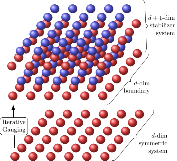
We propose a systematic framework to construct a (d+1)-dimensional stabilizer model from an initial generic d-dimensional abelian symmetry. Our approach builds upon the iterative gauging procedure, developed by one of the authors in [J. Garre-Rubio, Nature Commun. 15, 7986 (2024)], in which an initial symmetric state is repeatedly gauged to obtain an emergent model in one dimension higher that supports the initial symmetry at its boundary. This method not only enables the construction of emergent states and corresponding commuting stabilizer Hamiltonians of which they are ground states, but it also provides a way to construct gapped boundary conditions for these models that amount to spontaneously breaking part of the boundary symmetry.
In a detailed introductory example, we showcase our paradigm by constructing three-dimensional Clifford-deformed surface codes from iteratively gauging a global 0-form symmetry that lives in two dimensions. We then provide a proof of our main result, hereby drawing upon a slight extension of the gauging procedure of Williamson. We additionally provide two more examples in d=2 in which different type-I fracton orders emerge from gauging initial linear subsystem and Sierpinski fractal symmetries. En passant, we provide explicit tensor network representations of all of the involved gauging maps and the emergent states.
Introduction
Different incarnations of bulk-boundary correspondence are ubiquitous in condensed matter physics. Generically, a bulk-boundary correspondence establishes a relation between the non-trivial physics in the bulk of a certain physical system and the physics constrained to its boundary. One example of such a relation is the conjecture that the bulk of certain anomaly-free topological orders is fully determined by their gapped boundary theory by means of an appropriate notion of the categorical center Kitaev and Kong (2012); Kong and Wen (2014); Kong et al. (2017). A bulk-boundary correspondence has also proven to be the key for finding cohomological invariants that differentiate certain symmetry-protected topological phases (SPTs) protected by an invertible symmetry, whereby these invariants pertain to the transformation properties of the edge modes under the symmetry group. For the particular case of (1+1)d, this approach has led to a complete classification of gapped one-dimensional phases with group-like symmetry Chen et al. (2013); Schuch et al. (2011). More recently, it has also been argued how the boundaries of particular fracton phases host emergent subsystem symmetries whose explicit realization can be traced back to the characteristics of the bulk excitation spectrum Schuster et al. (2023). Contrary to the case of intrinsic topological orders, it was demonstrated that the bulk reconstruction of the fracton orders under scrutiny depends in a non-trivial way on the relative orientation of the boundary with respect to the bulk. In a certain sense all of the above examples of bulk-boundary correspondence can thus be brought together under the umbrella term of a holographic principle.
In another recent series of developments an opposite avenue has been pursued in which a given quantum field theory (QFT) with a (higher) categorical symmetry is regarded as an interval compactification of a topological field theory in one dimension higher, coined ‘SymTFT’, with a topological gapped boundary condition determining the symmetry of the QFT and a not necessarily gapped physical boundary condition that dictates the dynamics of the QFT Apruzzi et al. (2023); Kaidi et al. (2023). In this picture the focus is very much on the understanding of certain features of the symmetric QFT, such as (dis)order parameters, gapped phases and anomalies, from the higher-dimensional SymTFT. Aspects of this paradigm have previously appeared under the name of ‘strange correlator’, which admits an explicit lattice realization in terms of tensor network representations of the higher-dimensional topological order You et al. (2014); Vanhove et al. (2018, 2022).
In this manuscript we realize an explicit bulk-boundary correspondence for generic abelian boundary symmetries in any dimension by making use of the iterative gauging procedure proposed by one of the authors in Garre-Rubio (2024) for one-dimensional abelian boundary symmetries. That work builds on the observation that gauging an initial abelian (anomaly-free global 0-form) symmetry gives rise to dual on-site global symmetry generators labeled by the one-dimensional representations of the underlying symmetry group. Being itself free of any ’t Hooft anomaly, this emergent symmetry can be gauged so as to recover the initial symmetry. The crux of the paradigm put forward in Garre-Rubio (2024) is that these gauging procedures can be repeated indefinitely and that in this way a state emerges which naturally lives in one dimension higher than the initial symmetry. Such an emergent state was shown in Garre-Rubio (2024) to be stabilized by certain local operators whose origin can be traced back to the Gauss constraints of the involved gauging procedures. In this picture, the initial symmetry which is being gauged can be thought of as a boundary symmetry for the emergent state. This idea is made very tangible by making use of the explicit gauging map for quantum states proposed in Haegeman et al. (2015) and generalized later in Williamson (2016). One of the main advantages of using this approach is that a tensor network description of the gauging maps is readily available, which can in turn be used to write down an explicit tensor network representation of the emergent state, facilitating the analytical study of its properties and its numerical simulation.
In the current manuscript, Ref. Garre-Rubio (2024) is extended to arbitrary dimensions and generic abelian symmetries. Specifically, we propose a slight generalization of the gauging procedure of Williamson (2016) to arbitrary abelian groups, and demonstrate that the iterative gauging procedure of Garre-Rubio (2024) in any dimension gives rise to emergent states with corresponding local stabilizer Hamiltonians. The abelian symmetries which are being gauged in the framework of Williamson (2016) are completely specified by a complete collection of ‘checks’ which commute with all symmetry generators. As such, that framework includes the gauging of fractal and subsystem symmetries as specific cases. In our general framework we are also able to relate inequivalent choices of gapped boundary stabilizers to different spontaneous symmetry breaking patters of the boundary symmetry.
To showcase our framework we provide three detailed worked examples where the initial boundary symmetry is two-dimensional. Gauging a global on-site 0-form symmetry in (2+1)d gives rise to emergent 1-form – or Wilson loop– symmetries. In this case the iterative gauging framework gives rise to three-dimensional Clifford-deformed surface codes Huang et al. (2023), which are up to a local basis change equivalent to the three-dimensional abelian quantum doubles Kitaev (2003). Two-dimensional linear subsystem symmetries map to dual linear subsystem symmetries on the dual lattice. Applying the framework in this case gives rise to foliated anisotropic type-I fracton orders Shirley et al. (2020). Finally, we leverage the full potential of our framework and the gauging procedure of Williamson (2016) to gauge fractal boundary symmetry, specifically of Sierpinski type, and obtain the fracton model proposed by Caselnovo and Chamon in Castelnovo and Chamon (2012) for the study of quantum glassiness. For each of these examples we also provide a tensor network description of the involved gauging maps, and hence the emergent state, which is based on the tensor network description of the gauging map for global on-site 0-form symmetries of Haegeman et al. (2015).
Our manuscript is organized as follows. In section I we provide an introductory example to explicitly demonstrate the iterative gauging procedure applied to an initial two-dimensional global on-site symmetry. All the details of our framework including the study of symmetry-breaking boundary conditions and the tensor network representation of the emergent Clifford-deformed CSS codes are discussed in detail. This section also serves as an introduction to many of the conventions and notations used throughout this manuscript. We then proceed by putting these observations on systematic footing in section II. First, we slightly generalize the gauging procedure of Williamson (2016) to generic abelian groups and then prove that the iterative gauging procedure in any dimension gives rise to emergent states with a corresponding commuting stabilizer Hamiltonian of which it is a ground state. We then provide a way to add boundary stabilizers to the emergent Hamiltonian which commute with all terms in the bulk and among each other, thereby preserving the gap. We argue that different gapped boundary stabilizers correspond to certain symmetry breaking patterns of the boundary symmetry. We then conclude with two more examples in section III and section IV that pertain to the derivation of different type-I fracton models from the iterative gauging of linear subsystem boundary symmetry and fractal symmetry respectively.
I Introductory example:
Clifford-deformed surface codes from abelian topological symmetries
In this section we review the gauging procedure of abelian on-site global 0-form symmetries proposed in Haegeman et al. (2015) for two-dimensional symmetric states. We argue that the gauged state is in the even sector of a dual global 1-form symmetry acting non-trivially solely on the introduced gauge degrees of freedom. We use an explicit gauging procedure for this 1-form symmetry, following Rayhaun and Williamson (2023); Williamson (2016), that yields in turn again the original symmetry. We show that the concatenation of these 2D gauging maps as in Garre-Rubio (2024) produces 3D Clifford-deformed surface codes Huang et al. (2023), which are unitarily equivalent to abelian quantum doubles Kitaev (2003).
Let us consider the two-torus endowed with a lattice , whose sets of vertices, oriented edges and plaquettes will be denoted by , and respectively. The starting point of the gauging procedure laid out in Haegeman et al. (2015) is then a two-dimensional state living in a tensor product Hilbert space of matter degrees of freedom supported on the vertices of , . The local Hilbert space forms a unitary representation of , which is assumed to be abelian throughout the manuscript, and whose matrix representation is written as , . The state is required to transform trivially under the tensor product representation , i.e. , .111Indeed, if transforms non-trivially under , the gauging map defined below annihilates . However, a different gauging map can be defined for each symmetry sector.
Notice that the symmetry operators considered here act on all matter degrees of freedom , , simultaneously. Such a global symmetry is in modern jargon known as an invertible global 0-form symmetry Gaiotto et al. (2015). Here and below, for , a ‘q-form’ operator is a topological operator that acts non-trivially only on a codimension q submanifold of the spatial manifold, i.e. the two-torus. The case of the symmetry operators then naturally corresponds to .
For the sake of being concrete we will henceforth make an explicit choice of local Hilbert space and its representation. To this end we consider the character group of and choose the local Hilbert space as where is endowed with the inner product . This local Hilbert space is then assumed to carry the -representation defined as , . Let us also define .
I.1 Review: gauging two-dimensional abelian 0-form symmetries
Gauging a global on-site 0-form symmetry à la Haegeman et al. (2015)222Notice that the framework of Haegeman et al. (2015) applies more generally to non-abelian groups as well. The gauged theory in that case enjoys Wilson loop symmetries labeled by representations of the symmetry group. Wilson loops corresponding to higher-dimensional representations of the group can be realized on the lattice by non-trivial matrix product operators Lootens et al. (2021). begins with supplementing the Hilbert space with gauge degrees of freedom supported on the edges and valued in , . On this enlarged Hilbert space we define a gauge transformation for every vertex and every :
| (1) |
Here, , respectively , stands for the set of edges of that point into, respectively point out from, the fixed vertex , and we have introduced the operators
| (2) | ||||
| (3) |
For future reference we note that these operators satisfy the following algebra:
| (4) |
Notice that the operators in eq. 1 form a local representation of in the sense that they are supported on a small neighborhood around and obey for every and for every . Moreover, notice that the global symmetry operator is recovered by taking the product of the local symmetry operators on all vertices, namely
| (5) |
Next, a local projector is obtained by averaging over :
| (6) |
Indeed it is straightforward to verify that , by a relabeling of summation variables.
The commutation of the local projectors allows us to unambiguously define the global projector onto the gauge invariant subspace of the enlarged Hilbert space:
| (7) |
The state is then gauged by applying the projector to the initial state coupled to a trivial flat gauge field . Hence, we define the gauging map for the global 0-form symmetry as:
| (8) |
and the gauged state is by definition . Notice that by virtue of , which follows directly from a renaming of summation variable in the definition of , the local operators represent a local symmetry of the gauged state. It is exactly in this sense that this gauging procedure localizes the global 0-form symmetry. Furthermore it follows from that the gauging map projects out states which transform non-trivially under the global symmetry . As such, has a non-trivial kernel spanned by states in the original matter Hilbert space which are charged under the symmetry.
As mentioned in the introduction, the gauged states exhibit at least a global 1-form symmetry as a consequence of the imposed Gauss laws. This 1-form symmetry is the topic of the next section.
A final tangential comment which is of importance for what follows is in place. As argued in Haegeman et al. (2015) it is possible to disentangle the initial matter degrees of freedom from the newly introduced gauge degrees of freedom by means of a finite depth unitary quantum circuit, rendering the Gauss constraints trivial and effectively freezing the matter degrees of freedom to the eigenstate of . As showcased below; we will construct a three-dimensional state by concatenating gauging operators, wherein the ‘matter’ degrees of freedom in every layer will play the role of physical degrees of freedom of the three-dimensional state. We therefore refrain from applying this unitary circuit.
I.2 The dual 1-form symmetry
Let be an oriented closed path supported on the edges of the lattice . We define the following Wilson loop operators acting exclusively on the gauge degrees of freedom:
| (9) |
Here, is defined so that if the orientation of and coincide and otherwise. We can check that for every such loop this line operator commutes with the local gauge transformations:
| (10) |
To prove this, first notice that if and overlap, they overlap in an even number of edges. Let us consider just the case of two overlapping edges that we call , . Then for the given vertex , if both , have the same orientation as or both have the opposite orientation as , commuting through yields two cancelling phases and by virtue of the definition of and eq. 4. If on the other hand has the same orientation as but has the opposite orientation as , then we also obtain, due to the relative difference in orientation, phases and that cancel.
From eq. (10) together with the fact that we can conclude that
| (11) |
This implies that the gauged state transforms trivially under for every valid choice of and every character . Making use of the fact that , , it follows that the operators , with same , multiply according to the product of characters in , i.e.:
| (12) |
Also note that the operators are invariant under continuous deformations of , rendering them topological. These observations demonstrate that after gauging a global 0-form symmetry, an emergent global 1-form symmetry emerges.333In fact, one should think of the emergent 1-form symmetry, or more precisely symmetry, as being the invertible component of the full symmetry structure of the gauge theory. The complete symmetry structure was shown to constitute the 1-form symmetry together with all its 0-form condensation descendants and is organized in the fusion 2-category Roumpedakis et al. (2023); Lin et al. (2022); Bartsch et al. (2024); Bhardwaj et al. (2022); Delcamp and Tiwari (2024). Alternatively, one could think of (11) as a kinematical constraint satisfied by all allowed states in the gauge invariant Hilbert space.
I.3 Gauging the dual 1-form symmetry
Since the emergent 1-form symmetry is realized on-site, it is anomaly-free in the sense of Wen (2019) and can hence be gauged. To this end we use a similar procedure as in Haegeman et al. (2015); Rayhaun and Williamson (2023); Williamson (2016). After gauging this 1-form symmetry one expects the original 0-form symmetry to re-emerge Gaiotto et al. (2015); Rayhaun and Williamson (2023).
Following Rayhaun and Williamson (2023); Williamson (2016); Moradi et al. (2023), gauging of the 1-form symmetry happens via introduction of gauge degrees of freedom on the vertices of the lattice valued in the group algebra .444By invoking a form of Poincaré duality, one can identify the vertices of the primal lattice with the plaquettes of the dual lattice , i.e. . In that sense the gauge field can indeed be thought of as a 2-form gauge field for the global 1-form symmetry Moradi et al. (2023). A local 1-form gauge transformation for every edge is then constructed as follows:
| (13) |
where we used an analogue notation to the one in eq. 1 denoting by the vertex which is the target of and the source vertex of the edge . Naturally, is defined as . Akin to the case of the gauging of a global 0-form symmetry, these operators form a local representation of supported near , , . Notice that the global 1-form symmetries can be recovered by taking the (oriented) product of the 1-form gauge transformations along the loop , i.e.
| (14) |
, akin to eq. 5.
Group-averaging over allows us to construct the local projectors
| (15) |
where we made use of . From these we construct the global projector onto the gauge invariant subspace as:
| (16) |
Gauging the 1-form symmetry then ultimately happens in a similar fashion as in the 0-form case. We construct a gauging map by initializing all newly introduced gauge degrees of freedom in the trivial representation followed by acting with the projector onto the gauge invariant subspace:
| (17) |
Let us draw attention to the fact that without loss of generality the gauging map has as its domain only the edge degrees of freedom. This can be traced back to the fact that the emergent 1-form symmetry generators only act (non-trivially) on these degrees of freedom.
Completely analogous to the case of gauging a 0-form symmetry, the local symmetry exists by virtue of and manifests itself in the gauge invariant subspace as
| (18) |
for all and every .
Remark that by a renaming of summation variables in the definition (16), it follows that
| (19) |
for all closed paths and . In other words, the gauging map annihilates states which are not in the even sector of the global 1-form symmetry.
Finally and crucially, after gauging the 1-form symmetry the initial global 0-form symmetry reappears as anticipated. Indeed, it is found that
| (20) |
for all . Let us verify this. First note that for two vertices which share an edge commutes with the gauge transformation , by virtue of the identity
| (21) |
Combined with the observation that , we recover indeed eq. 20.
I.4 3D local symmetries from iterative gauging
Constructing a three-dimensional state from the above gauging maps now happens as follows. We start by choosing a two-dimensional state that will serve as the boundary condition of the three-dimensional state and fixing a choice of abelian group . We assume, as anticipated above, that this state lives in and transforms trivially under the abelian 0-form symmetry , i.e. , . Throughout the above discussions was kept completely general, and as such the construction that follows also can be applied to this most general case.
On we can thus first act with the gauging operator defined explicitly in (8), thereby introducing degrees of freedom valued in and supported on the edges of . Indeed, recall that acts according to , in which and stand for tensor products over the vertices and edges of the lattice. The gauged state has then as argued in section I.2 an emergent dual 1-form symmetry which is completely supported on the edges of and that in turn can be gauged using the procedure outlined in section I.3. Notice that the gauging map for this 1-form symmetry, defined in (17), acts only on the -valued degrees of freedom supported on the edges, leaving the original ‘matter’ degrees of freedom on the vertices valued in untouched. With slight abuse of notation: . In turn we can then again gauge the emergent 0-form symmetry that arises after the application of using the gauging map . In this step does not act on the degrees of freedom in living on . By repeatedly concatenating the gauging maps and we thus in every step are left with degrees of freedom in and which are not acted upon by the next gauging map. These are the degrees of freedom which, following the paradigm of Ref. Garre-Rubio (2024), are interpreted as physical degrees of freedom of a foliated three-dimensional state whose 2D layers are made up of the ‘matter degrees of freedom’ in every application of the gauging maps. Formally reads:
| (22) |
The exact meaning of the subscripts will be explained momentarily.
For concreteness we specialize to the square lattice henceforth. It can then be argued that the physical degrees of freedom of naturally organize themselves on the edges of a three-dimensional cubic lattice that we will denote by , and where the initial two-dimensional state serves as a physical boundary of the lattice.
We therefore consider the cubic lattice as being made up of alternating layers of vertical edges followed by a layer of horizontal edges, that we label by and respectively. The cubic lattice hence has a physical boundary made up of vertical edges.
For every layer of vertical edges we associate then these edges with the vertices of a copy of and the corresponding -valued ‘matter’ degrees of freedom that are not acted upon by the gauging maps . Analogously, we associate with every horizontal edge the degrees of freedom that are not touched by the ’s.
Using a blue color for edges that carry a copy of the local Hilbert space and red for those with a copy of , one can depict the cubic lattice away from the boundary as follows:
| (23) |
By virtue of the local symmetries of all the gauging maps appearing in eq. 22, the obtained state also inherits those local symmetries in a slightly modified way. It turns out that this prevents from being a trivial stacking of two-dimensional states as in fact the presence of these local symmetries translates to non-trivial entanglement between the degrees of freedom living in subsequent layers of the cubic lattice.
The result is that the emergent state is stabilized by plaquette operators for every plaquette of the cubic lattice, coming from the localization of the -form symmetry, and vertex operators for every vertex, from gauging the global -form symmetry. We denote the plaquette stabilizers by which are labeled by :
| (24) | ||||
| (25) | ||||
| (26) |
and the vertex stabilizers carry a group label :
| (27) |
Explicitly, the plaquette and vertex terms are given by
| (28) | ||||
| (29) | ||||
| (30) | ||||
| (31) |
Let us first show that stabilizes . To this end we single out one plaquette term supported on an -plaquette. From the commutation relation (21) together with the definition of in terms of the local gauge transformations (1), it follows that
| (32) |
Recognizing then as the local 1-form gauge transformation (13), which leaves invariant, together with the fact that proves that is a stabilizer of the state. The -plaquette terms can be derived in a similar fashion.
The final -plaquette terms can be recognized as the (minimal) global 1-form symmetries of the gauging map. Similarly, one can check that applied to maps to which is exactly the local symmetry of .
These observations allow us to consider the state a ground state of the commuting projector bulk Hamiltonian (a stabilizer code):
| (33) |
In this expression the sum over is over all vertices of the cubic lattice, and the sums over are over plaquettes in the , and planes respectively. The projectors are explicitly given by
| (34) |
and
| (35) | ||||
| (36) | ||||
| (37) |
It turns out that the Hamiltonian in eq. 33 is unitarily equivalent to the abelian quantum double Kitaev (2003). In its displayed form (33) it appeared previously in Huang et al. (2023) under the name of Clifford-deformed surface code. It can be brought in its more familiar form Kitaev (2003) defined on by applying the generalized Hadamard transformation
| (38) |
to every vertical edge carrying a copy of , as it can be checked that
| (39) | ||||
| (40) |
I.5 Symmetry breaking boundaries
The local stabilizers analyzed so far act on the bulk of the three-dimensional state . In this section we study the boundary stabilizers. These naturally are given by a subset of truncated bulk stabilizers commuting with the bulk stabilizers and defined above, where the subset depends on the choice of the boundary state , in particular the way in which is invariant under the 0-form symmetry. Indeed, for every choice of subgroup one can construct explicitly a -symmetric boundary state for which is a ground state of the bulk Hamiltonian (33) plus additional boundary terms which are projectors and which all commute with the terms in (33) and among themselves.
Let us proceed by constructing these boundary states and the corresponding boundary Hamiltonian terms explicitly. To this end we first define the following operators near the boundary (effectively truncating ) for any :
| (41) | ||||
| (42) |
These terms commute both with the bulk vertex operators and plaquette operators . Naturally, they also commute all among each other. From the explicit form of the gauging maps and it follows that given an irrep the operators (41-42) are stabilizers of if and only if , equivalently
| (43) |
for neighboring vertices . Notice that is an order parameter for the (partial) breaking of the global 0-form symmetry. Its expectation value is a two-point symmetric correlation function.
In what follows we show that given a choice of subgroup , is a stabilizer of for an appropriate boundary state depending on that subgroup, provided that is trivial when restricted to . It is a fact that characters in that are trivial when restricted to form a subgroup of isomorphic to . From now on we will abuse notation and denote this subgroup simply by . For the chosen subgroup we then propose following boundary state . First, we define the normalized states
| (44) |
Notice that is stabilized by in the sense that for all . Given we define
| (45) |
By construction is symmetric under the 0-form symmetry and, as anticipated, is symmetric under since leaves invariant and commutes with . Notice one can think of as an equal weight superposition of the ground states of a symmetric Hamiltonian whose symmetry is spontaneously broken down to . It is therefore meaningful to refer to these boundaries as symmetry breaking boundaries. We also define the following operators acting on the boundary:
| (46) |
which are symmetries of , and which commute with only if . Defining then
| (47) | ||||
| (48) | ||||
| (49) |
the Hamiltonian in the presence of such boundary terms reads
| (50) |
where the dependence on the choice of subgroup is explicit. As an example, one can consider the extreme cases of and that can be identified with Dirichlet and Neumann boundary conditions respectively. In the context of lattice gauge theory as of here it is also customary to refer to these cases as realizing the smooth and rough boundary conditions. 555Notice that we don’t recover twisted boundary conditions that amount to pasting an SPT phase on top of the symmetry broken boundary phase Wang et al. (2018a, b); Ji et al. (2023); Luo (2023); Zhao et al. (2023). It is expected that all such boundary conditions, which are in one-to-one correspondence with pairs , are recovered by appropriately twisting the boundary terms akin as in the lower-dimensional setting Garre-Rubio (2024); Wang et al. (2018b). This is most easily facilitated for by the triangular lattice.
As a final comment we consider an analogous construction of a three-dimensional state with a corresponding stabilizer Hamiltonian, which is constructed by starting from a state invariant under a -form symmetry generated by the Wilson loop operators (9):
| (51) |
The boundary terms in that case are given by truncating and :
| (52) | ||||
| (53) | ||||
| (54) |
Given a , is a symmetry of if and only if
| (55) |
Similarly as in the previous case one could define hosting a (partial) symmetry breaking phase of the 1-form symmetry with unbroken symmetry group . Commuting boundary stabilizers for such a state are given by
| (56) | ||||
| (57) |
Notice thus in particular that can host non-trivial 2D topological order. It is understood that besides these boundaries and the symmetry breaking ones considered above, it is also possible to define additional gapped boundaries which amount to (trivially) stacking a 2D topological order or stacking a 2D topological order while condensing composites of boundary anyons of the emergent state and (bulk) anyons from the stacked topological order Luo (2023).
I.6 Tensor network representation
As it turns out, the gauging maps and presented above can be naturally realized in terms of tensor networks, namely projected entangled-pair operators (PEPOs), of bond dimension Haegeman et al. (2015). For concreteness we restrict to the square lattice throughout this section. We comment below on the generalization to generic lattices.
Let us begin by introducing the tensors needed for the PEPO representation of . For every vertex of the lattice we introduce the rank 6 ‘vertex tensor’, or ‘Z-type tensor’
| (58) |
Notice that we use curly brakets, , to denote basis vectors and their duals on the virtual level. In order to implement the flat gauge field supported on the edges of the lattice we consider the rank 3 ‘+-type’ tensors
| (59) |
One unit cell of the tensor network representation of on the square lattice is obtained as follows
| (60) |
In this construction it should be understood that the full PEPO on the torus is obtained by placing copies of this unit cell on all vertices of the lattice and contracting along the virtual red legs. The analogue PEPO acting on a completely generic lattice is constructed by mirroring the above construction and placing on every vertex a more general Z-type tensor with a number of virtual legs which is equal to the degree of the corresponding vertex in the lattice. The edge tensors are unaltered. Contraction of the vertex and edge tensors then happens via the connectivity of the lattice.
One of the upshots of providing PEPO representations for the gauging maps is that their (global) symmetry properties automatically follow from the (local) symmetry properties of the local tensors from which the PEPO is made up. It follows readily from its definition that the vertex tensor satisfies
| (61) |
whereas the edge tensor obeys the relations
| (62) |
Consider first gauge invariance of the gauging map, that is for all and . This follows immediately from combining the second relation in eq. 61 with both identities in eq. 62 and noticing that all ’s on the virtual level exactly cancel with each other. The fact that on the other hand follows from application of the first identity in eq. 61 on every vertex together with the invariance of the edge tensors, namely
| (63) |
which is deduced from eq. 62.
Let us now proceed by showcasing the tensor network representation of the gauging map . In a similar vein as for the previous gauging map, we introduce tensors that will be placed on the edges of the lattice that read
| (64) | |||
| (65) |
Tensors incorporating the flatness of the (2-form) gauge field introduced on the vertices are then
| (66) |
Their relevant symmetry properties are:
| (67) |
and
| (68) |
Gauge invariance which in this case reads is a direct consequence of the second equality in eq. 67 combined with the identities of the vertex tensor in eq. 68. The property follows from the first equation in eq. 67 and the invariance properties of the vertex tensor, one of which reads:
| (69) |
This is not an independent property as it can be derived immediately from eq. 68.
Combining these tensors in a unit cell then results in a PEPO whose unit cell is given by
| (70) |
where, as alluded to above, the blue +-type tensors are placed on the vertices.
Combining now these PEPOs directly results in a tensor network representation of the emergent state , opening up the possibility for numerical simulation of the emergent state and further analytical study.
II General framework
What are the main takeaways from this introductory example? From iteratively gauging a global abelian 0-form symmetry and its dual 1-form symmetry we obtain stabilizer codes (local commuting projector Hamiltonians) in one dimension higher. Moreover, the obtained codes can be readily extended to include gapped boundary terms, and we have written down the states explicitly in terms of tensor networks.
The goal of this section is to provide a general framework for iteratively gauging a state which is symmetric under a certain collection of abelian symmetries defined via certain ‘check operators’ which commute with them. Hereby we extend the formalism of Williamson (2016) to arbitrary abelian groups. We argue that in this framework the concatenated gauging maps generically exhibit local symmetries originating from the Gauss constraints of the symmetries under scrutiny. These local symmetries can in turn be organized in an emergent local commuting projector Hamiltonian that naturally lives in one dimension higher than the initial state which is being gauged. Towards the end of this section we comment on the inclusion of the boundary terms in the emergent Hamiltonian which can be identified with certain spontaneous symmetry breaking patterns of the boundary symmetry realized by . Since these gauging maps can be defined in any dimension, we recover the results from Garre-Rubio (2024) as a particular case.
II.1 Gauging abelian symmetries
To set the scene we assume a lattice in which each vertex supports a copy of . The tensor product Hilbert space will be written as henceforth. Notice that we don’t make any assumption about the underlying topology or dimension of the spatial manifold on which is defined.
Throughout this section we deal with symmetry operators that are fully specified by a complete collection of ‘check operators’, labeled , that commute with all of them. The formal gauging procedure of Williamson Williamson (2016) then happens via the introduction of a gauge degree of freedom for every such check. Formally, consider for any the operators
| (71) |
where is a subset of the vertices, i.e. . Borrowing the notation of Williamson (2016), we will denote by a multivalued function that maps a given constraint from the collection , that will below be identified with the gauge degrees of freedom, to a corresponding set of vertices . Furthermore we introduce the involution which evaluates to or depending on the relative orientation of the constraint and the vertex . An operator is then a valid symmetry generator if it commutes with the checks
| (72) |
for all and all . Below, we will sometimes refer to the symmetry generated by these valid symmetry generators as the ‘initial’ symmetry.
To connect with the previous section, let us remark that the global 0-form symmetry corresponds to the case , and thus . For these symmetry generators the checks can be chosen so that there is exactly one check per edge of the lattice, i.e. . Explicitly, the checks then read , where we refer to the previous section for a detailed explanation of the notation.
An important observation is that the local constraints can be interpreted as local Hamiltonian terms that commute with the symmetry Williamson (2016). As such, they can be used to construct generalized Ising models and when perturbed, for example with single-vertex terms, they host symmetry breaking phases of such symmetries.
We now proceed by gauging the symmetry generated by the operators , essentially mimicking the procedure used in the previous section based on Haegeman et al. (2015); Williamson (2016) adapted to this more general setting. To this end we first enlarge the ‘matter’ Hilbert space with a -valued gauge degree of freedom for every check in . We will denote the physical support of the gauge degrees of freedom by where it has to be understood that there is bijection between and . Typically, can be identified with a (subset) of k-cells of the lattice rendering the aforementioned bijection canonical.
Having again the example from the previous section in mind, can thus be identified with as anticipated above.
Writing , the first step of the gauging procedure thus entails enlarging according to . Given the map defined above, we define as the preimage of under . In other words, maps the matter degree of freedom localized on to its associated gauge degrees of freedom. In light of the above identification of gauge degrees of freedom and constraints, we will also interpret the set of constraints as its corresponding subset of . We then define the gauge transformation on the enlarged Hilbert space as:
| (73) |
Out of these gauge transformations, a local projector is constructed by taking the -average:
| (74) |
. Indeed remark that from a redefinition of summation variables it follows that for all .
The gauging map is then finally defined as the operator obtained by acting with the local projectors on the trivial gauge field :
| (75) |
Let us summarize the most important properties of before proceeding. We refer to Williamson (2016) for a more detailed digression. For a given , the gauge transformations form a local -representation in the neighborhood of , in the sense that , . It then follows from the definitions that . By a relabeling of summation variable in the definition of it also follows immediately that for all allowed symmetry operators. As illustrated in section I this property implies that only states transforming trivially under the symmetry, i.e. , and for all allowed , are gaugeable. Given such a state, we coin the gauged state. From it readily follows that the gauged state is gauge invariant as expected. Even though we only deal with gauging states throughout this manuscript, it should be noted that also operators can be gauged using this prescription. In particular, local and symmetric operators in the initial matter theory are mapped to dual local gauge-invariant operators under the gauging procedure in such a way that the matrix elements of these symmetric operators w.r.t. a symmetric state are preserved.
As an example, consider once more the case of a 0-form symmetry. Notice that with the choices of relative orientations implicitly defined above, we recover the Gauss constraints defined earlier in eq. 1, from which eventually the gauging map given in eq. 8 of Haegeman et al. (2015) is recovered.
Crucially, the gauge theory obtained via the aforementioned proposal exhibits global ‘emergent’ symmetries that, by construction, are anomaly-free and hence gaugeable Wen (2019). Let us continue by identifying these emergent symmetries. First notice that even though the constraints do not commute with the gauging map, the dressed constraints do commute with all Gauss operators and, a fortiori, with the gauging map . Indeed, this follows from a direct computation. For fixed and let us assume without loss of generality that , which necessarily implies that :
| (76) |
In the second line the definition of and was employed. In the third line we used the commutation relations eq. 4 and eq. 21. Combined with the fact that evaluates to on the trivial gauge field , this implies that the constraint for every and is the preimage of under the gauging map . In particular, it follows that for a choice of constraints and choice of involution , such that
| (77) |
there exists a corresponding operator in the gauge theory
| (78) |
which is an emergent symmetry of in the sense that
| (79) |
Applying the above to the example of (8) considered in section I, we note that eq. 77 is exactly satisfied for any choice which coincides with a closed loop supported on the edges of the lattice. With the above choice of , exactly takes the relative orientation of with respect to the orientation of the edges into account.
In order to gauge the emergent symmetry operators we adapt a similar approach as for the initial symmetry (71). Notice that the symmetry generators defined in eq. 78 commute with the local checks
| (80) |
which are naturally localized around the vertices . Therefore we will identify the set of these checks with the set of vertices . To prove that these checks indeed commute with the emergent symmetry generators, consider some vertex . The identity (77) guarantees the existence of constraints such that . It follows immediately that commutes with , from which the claim follows. In order to define the corresponding dual gauging map , we once more enlarge the Hilbert space according to , on which we define the Gauss operators
| (81) |
Notice the complex conjugate appearing in . Corresponding local projectors localized around follow from averaging over :
| (82) |
Ultimately the dual gauging map reads
| (83) |
It follows that after gauging these emergent symmetries using the gauging map the original symmetry is recovered, as expected. This is quickly demonstrated by noticing that all symmetry generators commute by definition with the checks , and by extension with the Gauss constraints , so that .
II.2 Concatenation of gauging maps
Let us now consider the composition of the gauging operators defined above. With slight abuse of notation we consider in this section thus the composed operators
| (84) |
and
| (85) |
Herein, stands for the number of vertices of the lattice and by definition is equal to the number of constraints defining the initial symmetry (71), i.e. . As anticipated above, these concatenated gauging maps exhibit local symmetries that can be traced back to the Gauss constraints enforced by and . Crucial in the derivation of the local symmetries are following identities which can be derived in a similar fashion as eq. 76:
| (86) | ||||
| (87) |
Given these identities, it is now straightforward to argue that the mutually commuting operators
| (88) | |||
and
| (89) | |||
are symmetries of the concatenated gauging maps and respectively. Indeed:
| (90) | ||||
| (91) |
for all , , , . The iterated gauging procedure put forward in Garre-Rubio (2024) now dictates that given any state stabilized by the initial symmetry, that is
| (92) |
for every valid symmetry operator , one can define the emergent state as
| (93) | |||
where the big tensor products run over all appearances of the gauging maps in the definition.
This state is then by construction stabilized by the operators and defined above. Given these stabilizers one can subsequently construct a stabilizer Hamiltonian for which is a ground state. Remark that additional stabilizers are given by the emergent symmetries of every gauging map. For the examples that follow we will refrain from including these stabilizers as they are in those cases non-local operators. However, note that this is by no means always the case. Recall that in the case of the emergent 1-form symmetries studied in section I, these emergent 1-form symmetries around individual plaquettes gave rise to the plaquette terms defined in eq. 30. In fact, we rather would like to think of these terms as kinematical constraints on the Hilbert space on which the emergent state is defined and as such we are allowed to include them in the Hamiltonian.
Given the foliated way in which the emergent state (93) is constructed it is now a sensible thing to consider this foliation as an additional dimension so that is a state that lives in exactly one dimension higher than the initial state . In this interpretation behaves as a boundary condition for the emergent state. The lattice on which is supported can then also be thought of as emerging from on which is defined. More precisely, the lattice is made up of layers which each carry a copy of . In every other layer -valued degrees of freedom are placed on and -valued degrees of freedom supported on . This is most easily demonstrated by concrete examples.
II.3 Gapped boundary conditions
In the interpretation of as a state living in one dimension higher than , the stabilizers and are interpreted as acting on the bulk of the state . The question of how to include boundary terms that stabilize poses itself. As it turns out, the answer to this question is intimately interwoven with the exact way in which the initial symmetry is realized on the boundary state .
Let us begin by considering the simplest local candidate stabilizer. It can be verified readily that for a given and
| (94) | |||
commutes with the gauging map since it obviously commutes with the local gauge transformations . Hence, it is a stabilizer of the emergent state exactly when it is one of the boundary condition, i.e. . Note that one could think of this operator as a ‘truncated’ vertex term .
Consider likewise the truncated term
| (95) | |||
Recall that the preimage of this operator under was shown to be
| (96) |
in eq. 87. This observation thus implies that the truncated term (95) is a stabilizer of the emergent state, whenever is stabilized by the check . Since these local constraints can be understood as local symmetric order parameters for the global symmetry (71), inequivalent boundary conditions realizing different symmetry breaking patterns of this symmetry can be devised. More formally, consider for any subgroup the state which we recall was defined in section I.5 as . Constructing then the tensor product state
| (97) |
it is clear that this reference state is stabilized by and provided that , and . Remember indeed from section I.5 that stands for the subgroup of characters in which are trivial when restricted to . From this it also follows that the corresponding boundary stabilizers of the emergent state commute. More generally, we could equally well consider boundary states of the form
| (98) |
for any allowed , which enjoy the same stabilizers.
Also remark that, depending on the specifics of the symmetry generators, even more generic boundary conditions can be defined, for example by also (partially) breaking the translational invariance of the boundary state. An exhaustive study of gapped boundary conditions for the models under scrutiny will be the topic of future work.
III Foliated Type-I Fracton order from 2D linear subsystem symmetries
In this section we showcase the gauging of abelian linear subsystem symmetries and their dual emergent symmetries, which are themselves linear subsystem symmetries on the dual lattice, following the prescriptions of section II. Concatenation of these gauging maps results in foliated type-I fracton codes, generalizing the anisotropic models studied in Shirley et al. (2020) defined for cyclic groups to arbitrary finite abelian groups.
III.1 Gauging 2D abelian linear subsystem symmetries and their emergent symmetries
Throughout this section we consider again the two-torus, now endowed with a square lattice denoted by . The initial -valued ‘matter’ degrees of freedom are located on the vertices as customary. It will be useful to express the vertices in terms of their Cartesian coordinates as . Naturally, and stand for the linear system size in the and direction respectively. The linear subsystem symmetry (LSS) generators are then represented on the matter Hilbert space as
| (99) | |||
| (100) |
There thus exists an extensive number of symmetry generators, one for every in the direction of the square lattice, , and one for every in the direction, . Notice however that not all of the symmetries generators are independent since clearly , .
Graphically, an example of symmetry operators and on a portion of the square lattice looks like:
| (101) |
In order to employ the recipe of the general framework laid out in section II we need to consider the checks that fully specify these symmetry generators. An adequate choice is given by
| (102) |
, . These operators are naturally associated with the plaquettes , and we will therefore henceforth identify the constraints with the plaquettes, i.e. . Indeed, graphically, one such operator can be depicted as
| (103) |
Let us continue by gauging this symmetry. Therefore we introduce thus -valued gauge fields on the plaquettes and thereby extend the Hilbert space according to , where . The local gauge transformations in the neighborhood of the vertex read then
| (104) |
for every . The tensor products appearing in this definition are over the sets of plaquettes , respectively , which ‘enter’, respectively ‘leave’, the vertex according to the following orientations:
| (105) |
As such, the definition of is in accordance with eq. 73. Notice that here the same blue and red color code of the previous sections for depicting degrees of freedom in respectively and is recycled. Evidently, the gauge transformations form a local -representation in the neighborhood of every vertex , i.e. , .
As prescribed by our general gauging procedure, we define the following local projector:
| (106) |
for every vertex , out of which we construct the projector onto the gauge invariant subspace as:
| (107) |
Gauging of the LSS then happens by initializing the gauge fields in the trivial tensor product configuration and applying the above projector so as to obtain
| (108) |
The notation , following Rayhaun and Williamson (2023), is motivated by the fact that there is a sense in which linear subsystem symmetries can be thought of as ‘-form’ symmetries: -form symmetries acting on a codimension foliation of the spatial manifold. The LSS symmetry is localized in the sense that , , . From the above definition of the gauging map it follows that it satisfies:
| (109) | ||||
| (110) |
, , . Hence, in line with the expectation from the general framework, states transforming non-trivially under one or more of the global linear subsystem symmetry generators are annihilated by the gauging map .
Let us now present the emergent symmetries. These happen to be themselves linear subsystem symmetries supported on the dual square lattice and are labeled by characters . Similarly as in the case of the initial LSS it proves useful to define the vertices of the dual square lattice, , in terms of their Cartesian coordinates, i.e. . Also notice that the dual vertices can be identified under Poincaré duality with the plaquettes of the primal square lattice, formally: . We then define for any character the dual LSS generators:
| (111) | |||
| (112) |
Examples of and then look like
| (113) |
wherein the dual lattice is drawn in gray on top of the primal lattice drawn in black.
The emergent symmetries are apparent from
| (114) | |||
| (115) |
for all .
Despite these identities being a mere application of eq. 79 to the case at hand, let us nevertheless derive these emergent symmetries explicitly for completeness. To this end, note that the operators commute with the projector in eq. 107 and leave invariant the initial trivial gauge field on the plaquettes . The former is satisfied because along dual horizontal and vertical directions , the operators overlap in two faces with the projectors appearing in the definition of that act as on them.
III.2 Iterative gauging of linear subsystem symmetries
Due to the structural similarity between the dual LSS generators (111, 112) and the initial ones (99, 100), the gauging procedure of the latter can be readily adopted to gauge the emergent LSS symmetries. To this end, we introduce -valued gauge fields on the plaquettes of the dual lattice , which, as we mentioned, can equivalently be thought of as the vertices . As is custom by now, we initiate these gauge fields as . On this enlarged Hilbert space we define the local gauge transformation
| (116) |
The orientations determining the sets of ‘incoming’ and ‘outgoing’ plaquettes on the dual square lattice, respectively and , are dual to those on the primal lattice as per the convention in (105). From the perspective of the primal lattice this gauge transformation can hence be depicted as
| (117) |
Using the local projectors
| (118) |
the following gauging map is then constructed:
| (119) |
After the application of LSSs on the primal lattice represented by (99-100) are reobtained. Hence, we can iteratively gauge an initial state that is in the even sector of the LSSs (99-100) using the usual prescription as follows
| (120) |
Following our general paradigm we then interpret as a (3+1)d state living on a cubic lattice endowed with a copy of to every edge in the direction ( blue) and a local Hilbert space ( red) associated to every plaquette in the -plane. It follows that the bulk stabilizers of the state can be pictorially represented as
| (121) | ||||
| (122) |
for every vertex and every cube respectively. The state (120) is thus a ground state of the commuting projector Hamiltonian
| (123) |
in which
| (124) | ||||
| (125) |
This generalizes the anisotropic model introduced in Shirley et al. (2020), which exhibits foliated type-I fracton order, to arbitrary finite groups. Our representation can be brought in the form showcased in Shirley et al. (2020) by applying the local basis transformation defined in eq. 38 to the red plaquettes. It is expected that our approach will facilitate the classification and construction of these fracton orders.
III.3 Boundary conditions
Let us now also extend the bulk Hamiltonian to the boundary of the three-dimensional cubic lattice. To this end we consider following operators near the boundary:
| (126) | ||||
| (127) |
for all and .
Being ‘truncated’ versions of the bulk stabilizers and , they naturally commute with all bulk terms appearing in the bulk Hamiltonian . Note that, similar as to the boundary terms defined for the introductory example in section I.5, and only commute for particular choices of and such that . This statement will be refined below.
From the general framework it follows that stabilizes the three-dimensional state if the boundary condition is symmetric under the operator
| (128) |
for the plaquette on the boundary corresponding to . One recognizes these operators as the checks defined above. For illustrative purposes, let us construct one particular reference boundary before proceeding to the more general case.
A suitable choice for is any of the extensive number of ground states of the two-dimensional classical Ising plaquette model. Indeed, recall that the Hamiltonian of this model is exactly given by . One such ground state is for example constructed by starting from the product state
| (129) |
where the notation introduced in eq. (44) was used, and acting on this reference state with all LSS generators according to
| (130) |
We stress that in this definition every summation over group elements is over the entire group . From the observation that for every , together with the fact that the checks commute by definition with all LSS generators, it indeed follows that is a good boundary condition for the emergent state for which additional boundary stabilizers are given by
| (131) |
Similar as to the introductory example in section I, and as per the general paradigm in section II, we can also define more general boundary conditions for different symmetry breaking patterns of the LSS on the boundary. Indeed, given again the state defined in eq. 44, it is natural to define
| (132) |
Given this choice of boundary condition, appropriate commuting boundary stabilizers are given
| (133) | ||||
| (134) |
Indeed given that , and thus for any , the boundary operators and defined in (126,127) commute. These boundary terms are then added to the bulk Hamiltonian (123) to obtain the Hamiltonian
| (135) |
Before proceeding we note that the boundary conditions presented here are by no means exhaustive. In particular it should be pointed out that the boundary states defined in eq. 132 are manifestly translationally invariant, which is a condition which can be relaxed Schuster et al. (2023). A complete study of all (gapped) boundary conditions for these models will be presented elsewhere.
III.4 Tensor network representation
Let us finalize our discussion with providing tensor network representations of the (dual) LSS gauging maps defined above. To this end we use tensors which slightly generalize those introduced in section I.6. Their symmetry properties are therefore also completely analogous and are not repeated here. Let us first show the PEPO corresponding to the gauging map defined in eq. 108. Again restricting to one unit cell of the PEPO, which in this case is made up of one Z-type tensor on the vertex of the unit cell and one -type tensor on an adjacent plaquette , we claim that the PEPO is constructed from:
| (136) |
Indeed, let us verify its relevant properties. In the first place it follows from eq. 61 combined with eq. 63 that the gauging map absorbs the initial LSSs supported on the vertices of the primal lattice, i.e. (109-110). Analogously, the gauge invariance of the gauging map, i.e. , , , is proven by making use of eq. 61 and (62). Finally, the existence of the emergent symmetries is a direct consequence of the ‘flatness’ of the gauge field enforced by the -tensors, combined with the observation that the Z-type tensors are diagonal in its virtual indices.
The PEPO representation of in turn is constructed from the unit cell
| (137) |
In this depiction it has to be understood that the dual Z-type tensor is placed on a plaquette of the lattice whereas the dual +-type tensor is located on a vertex . The symmetries of this PEPO are immediately found from dualizing those of the above PEPO defined in eq. 136; from them the properties of are recovered immediately.
IV Type-I fracton orders from 2D Fractal symmetries
In this section we consider Sierpinski fractal symmetry as initial symmetry to our iterative gauging procedure. It is shown that the original Castelnovo-Chamon fractal model proposed in Castelnovo and Chamon (2012) emerges.
IV.1 Gauging Sierpinski fractal symmetry and its emergent dual fractal symmetry
Let us begin by defining a set of generators for the fractal Sierpinski symmetry. Therefore we consider the two-torus endowed with a triangular lattice that we will denote by . Given a vertex , we will denote its rectangular coordinates in the basis , indicated in the figure below, by , ; being the linear system size. Every vertex carries a copy of the local Hilbert space on which the Pauli operators and are defined.666In fact, in the remainder of this section we will identify and by making use of the obvious isomorphism . We will consider a subset of the plaquettes whose member plaquettes are shaded in red in the figure below, foreshadowing that we will put gauge degrees of freedom on these plaquettes when gauging the fractal symmetry. Note that the number of such plaquettes equals the number of vertices, i.e. .777Indeed, this follows from the fact that the Euler characteristic of the torus is zero, which can be expressed as , combined with the facts that and . This allows us to assign to every a ‘base point’ which we conventionally choose as dictated by the dotted lines in the figure:
| (138) |
As pointed out in Devakul et al. (2019) the number of symmetry generators depends in a non-trivial way on the (linear) system size . In this section we will for demonstrative purposes restrict to the case of for an integer , in which case the number of symmetry generators is exactly equal to . The Sierpinski symmetry generators are then of the form
| (139) |
where is a function defined such that commutes with the checks which are given by
| (140) |
for all . A check thus consists of three Pauli operators acting on the three vertices surrounding a plaquette .
As follows from a direct computation, imposing commutation of the generators (139) with all these checks requires to satisfy the recursive identity
| (141) |
. A valid symmetry generator is hence fully specified by a valid choice of ‘initial condition’ at :
| (142) |
The function , for follows then from applying the recursion relation to this choice of , and as such the corresponding generator commutes by construction with all checks. independent choices for which give rise to the independent Sierpinski symmetry generators that we expect can be chosen as
| (143) |
Let us mention as a side remark that it turns out that one could think of as a valid history of a Sierpinski cellular automaton in the following sense. For fixed , corresponds to a state valued in . Given this state, the state at , i.e. for fixed , is fully specified by the above recursion relation from . Therefore can be thought of as labeling discrete ‘time’ steps, this notion of time thus flows in the direction of increasing . In this picture serves as an initial condition for the automaton, a posteriori justifying our jargon introduced above.
As a concrete example take , and . The corresponding history is then computed to be
| (144) |
whose matching lattice operator can be depicted as:
| (145) |
Let us now gauge the Sierpinski symmetry using the general paradigm of section II. To this end we introduce qubit gauge degrees of freedom on the plaquettes in . A local gauge transformation for every reads then
| (146) |
wherein the tensor product is understood to be over plaquettes that contain . Graphically:
| (147) |
From the local projector
| (148) |
one constructs, as is by now routine, the global projector from which one obtains the gauging map by trivially initializing the gauge field:
| (149) | |||
| (150) |
Evidently, one has . Let us also verify explicitly that this gauging map indeed projects out states transforming non-trivially under the Sierpinski symmetry, i.e. , for all valid symmetry generators defined in eq. 139. To this end, we could expand the local projectors appearing in the definition of the gauging map :
| (151) |
From the definition of in eq. 146 it then follows that three ’s in the expansion (151) on vertices , and overlap in exactly one plaquette , namely the one such that . Locally, this means that the property is equivalent to satisfying (141), which it has to in order to define a genuine Sierpinski symmetry generator.
We now turn to the emergent symmetries. As a matter of fact, after gauging we obtain a dual Sierpinski fractal symmetry supported on the gauge degrees of freedom. Given a plaquette , we define its ‘rectangular coordinates’ as . Mimicking the definition of , let us define by means of the recursive identity
| (152) | ||||
| (153) |
for all . By comparison with the definition of in (141) we can infer that defines a Sierpinski fractal symmetry in which the ‘time steps’ labeled by flow in the opposite direction compared to the one in (141) and in which the ‘spatial direction’ is reflected as well. It can then be shown that exactly specifies the emergent fractal symmetries after gauging. Namely, defining
| (154) |
it follows that
| (155) |
Indeed, this follows from the fact that exactly for this choice of the operator commutes with every , , together with the trivial observation that the initial flat gauge configuration is a eigenstate of .
IV.2 Iterative gauging
Gauging of the dual Sierpinski symmetry happens via the introduction of qubits on the vertices . In the neighborhood of a plaquette , following gauge transformation is defined:
| (156) |
which forms a local -representation. In this, stands for the set of three vertices surrounding . Concretely:
| (157) |
Based on the local projector, defined as
| (158) |
the corresponding gauging map reads:
| (159) |
in which . The expected properties and , for all valid symmetry generators and , hold by construction.
What is the emergent state obtained from these gauging procedures? It turns out that the emergent state can be interpreted as living on the vertices of a hexagonal close-packed (HCP) lattice, which consists of layers of triangular lattices whose vertices are slightly displaced with respect to each other Casasola et al. (2024). A slightly different realization of this lattice which is closer to our setup is the following. We consider also layers of two-dimensional triangular lattices , but in such a way that the vertices of all layers align along the direction perpendicular to the stack of layers. In every other layer we then place qubits on the vertices of the triangular lattice, i.e. on , and on the plaquettes . Using a blue color for the former degrees of freedom, and a red color for the latter, the bulk terms of the emergent Hamiltonian are then the following:
| (160) | ||||
| (161) |
With slight abuse of notation, refers to the vertex of the emergent lattice on which the bottom blue qubit appearing in the operator is supported. On the other hand, refers to the support of the red qubit on the bottom of the depiction of the operator. It is clear that these operators all mutually commute. We can construct projectors out of these operators as
| (162) | |||
| (163) |
The emergent bulk Hamiltonian then reads
| (164) |
where the sums are over all (bulk) vertices and -plaquettes of the HCP lattice. This model was proposed by Caselnovo and Chamon in Castelnovo and Chamon (2012), is covered in the family of models by Yoshida Yoshida (2013) and was recently studied in detail in Casasola et al. (2024).
If we start the iterative gauging by , the possible boundary terms correspond to the truncation of (160) near the boundary or individual terms. Explicitly the truncated (160) terms read:
| (165) |
which also have been identified and studied in Casasola et al. (2024). The term acts on the boundary state , with is symmetric under the fractal Sierpinski symmetry, as:
| (166) |
which can be recognised as the local checks and serve as a local order parameter for the initial fractal symmetry. As such, there are two possible boundaries depending on whether the fractal symmetry is spontaneously broken by or not. In the first case, the boundary stabilizers are given by
| (167) |
for all on the boundary , whereas in the symmetry breaking case the stabilizers are given by
| (168) |
IV.3 Tensor network representation
The tensor network representations of and are readily constructed by mirroring the PEPO constructions that have appeared in the previous examples. Since we are dealing with the symmetry group here, we can in fact significantly simplify the tensor network calculus introduced in section I.6 by removing the arrows and using a red color for all tensor legs since we have identified and above. By virtue of these simplifications, we will also only need two type of tensors for both gauging maps which are given by:
| (169) |
which in the construction of the -PEPO will be placed on every vertex and in the case of the -PEPO on every plaquette in , and
| (170) |
placed on the plaquettes when it appears in the PEPO representation of and on the vertices when it appears in the -PEPO.
For the PEPO representations of both gauging maps we make a choice of unit cell such that a plaquette tensor on a given is combined with a vertex tensor placed on the corresponding base point . For the gauging map , the PEPO unit cell is then explicitly given by:
| (171) |
where, as mentioned above, the +-type tensor is placed on a certain plaquette and the Z-type tensor on the corresponding base point . Analogously, the unit cell of the PEPO representation of can be depicted as
| (172) |
where now the Z-type tensor is placed on a plaquette and the second tensor on the corresponding base point.
In both cases it follows easily from the symmetry properties of the tensors, which can be derived from the identities given in section I.6 specialized to the case , that these gauging maps satisfy all required properties.
V Conclusion and Outlook
In this work we have put the iterative gauging paradigm of Garre-Rubio (2024) for abelian symmetries on a systematic footing and extended it to arbitrary dimensions and generic types of abelian symmetries. We provided explicit examples where the emergent states are three-dimensional. Concretely we have shown the emergence of surface codes and foliated type-I fracton codes from the iterative gauging of 0-form, 1-form, linear subsystem and Sierpinski fractal symmetry.
We predict a number of ways in which this framework can be further refined and propose the following open problems. From the case of the emergent surface codes, it is clear that further refinement is required to accommodate boundary conditions hosting SPT phases on top of the partial symmetry breaking. It is plausible that similar to the lower-dimensional case Garre-Rubio (2024) this requires modification of the boundary stabilizers. A similar question arises regarding the boundary conditions of the emergent anisotropic models studied in section III. In particular, it would be revealing to study boundaries that (potentially partially) break translation symmetry
One could wonder to what extent our framework is exhaustive in producing stabilizer codes. An obvious family of models not treated in this work are type-II fracton models, which differ from type-I fracton models in the mobility of their excitations. Adapting our approach to accommodate these fracton orders could prove to be a formidable challenge.
We further predict that the explicit tensor network constructions of the states provided here will enhance their numerical study. Immediate access to the boundary states in this framework could facilitate the study of boundary phase transitions of these models.
Acknowledgments
The authors thank Jacob Bridgeman, Clement Delcamp, Jutho Haegeman, Anasuya Lyons and Dominic Williamson for discussions and comments. This work has received funding from the Research Foundation Flanders (FWO) through Ph.D. fellowship No. 11O2423N awarded to BVDC. This work has been partially supported by the European Research Council (ERC) under the European Union’s Horizon 2020 research and innovation programme through the ERC-CoG SEQUAM (Grant Agreement No. 863476) and by the FWF Erwin Schrödinger Program (Grant No.J4796).
References
- Kitaev and Kong (2012) A. Kitaev and L. Kong, Commun. Math. Phys. 313, 351 (2012), arXiv:1104.5047 [cond-mat.str-el] .
- Kong and Wen (2014) L. Kong and X.-G. Wen, (2014), arXiv:1405.5858 [cond-mat.str-el] .
- Kong et al. (2017) L. Kong, X.-G. Wen, and H. Zheng, Nucl. Phys. B 922, 62 (2017), arXiv:1702.00673 [cond-mat.str-el] .
- Chen et al. (2013) X. Chen, Z.-C. Gu, Z.-X. Liu, and X.-G. Wen, Phys. Rev. B 87, 155114 (2013), arXiv:1106.4772 [cond-mat.str-el] .
- Schuch et al. (2011) N. Schuch, D. Pérez-García, and I. Cirac, Phys. Rev. B 84, 165139 (2011).
- Schuster et al. (2023) T. Schuster, N. Tantivasadakarn, A. Vishwanath, and N. Y. Yao, (2023), arXiv:2312.04617 [cond-mat.str-el] .
- Apruzzi et al. (2023) F. Apruzzi, F. Bonetti, I. García Etxebarria, S. S. Hosseini, and S. Schafer-Nameki, Commun. Math. Phys. 402, 895 (2023), arXiv:2112.02092 [hep-th] .
- Kaidi et al. (2023) J. Kaidi, K. Ohmori, and Y. Zheng, Commun. Math. Phys. 404, 1021 (2023), arXiv:2209.11062 [hep-th] .
- You et al. (2014) Y.-Z. You, Z. Bi, A. Rasmussen, K. Slagle, and C. Xu, Phys. Rev. Lett. 112, 247202 (2014), arXiv:1312.0626 [cond-mat.str-el] .
- Vanhove et al. (2018) R. Vanhove, M. Bal, D. J. Williamson, N. Bultinck, J. Haegeman, and F. Verstraete, Phys. Rev. Lett. 121, 177203 (2018), arXiv:1801.05959 [quant-ph] .
- Vanhove et al. (2022) R. Vanhove, L. Lootens, H.-H. Tu, and F. Verstraete, J. Phys. A 55, 235002 (2022), arXiv:2107.11177 [math-ph] .
- Garre-Rubio (2024) J. Garre-Rubio, Nature Commun. 15, 7986 (2024), arXiv:2403.07575 [quant-ph] .
- Haegeman et al. (2015) J. Haegeman, K. Van Acoleyen, N. Schuch, J. I. Cirac, and F. Verstraete, Phys. Rev. X 5, 011024 (2015), arXiv:1407.1025 [quant-ph] .
- Williamson (2016) D. J. Williamson, Phys. Rev. B 94, 155128 (2016), arXiv:1603.05182 [quant-ph] .
- Huang et al. (2023) E. Huang, A. Pesah, C. T. Chubb, M. Vasmer, and A. Dua, PRX Quantum 4, 030338 (2023), arXiv:2211.02116 [quant-ph] .
- Kitaev (2003) A. Y. Kitaev, Annals Phys. 303, 2 (2003), arXiv:quant-ph/9707021 .
- Shirley et al. (2020) W. Shirley, K. Slagle, and X. Chen, Phys. Rev. B 102, 115103 (2020), arXiv:1907.09048 [cond-mat.str-el] .
- Castelnovo and Chamon (2012) C. Castelnovo and C. Chamon, Phil. Mag. 92, 304 (2012).
- Rayhaun and Williamson (2023) B. C. Rayhaun and D. J. Williamson, SciPost Phys. 15, 017 (2023), arXiv:2112.12735 [cond-mat.str-el] .
- Gaiotto et al. (2015) D. Gaiotto, A. Kapustin, N. Seiberg, and B. Willett, JHEP 02, 172 (2015), arXiv:1412.5148 [hep-th] .
- Lootens et al. (2021) L. Lootens, J. Fuchs, J. Haegeman, C. Schweigert, and F. Verstraete, SciPost Phys. 10, 053 (2021), arXiv:2008.11187 [quant-ph] .
- Roumpedakis et al. (2023) K. Roumpedakis, S. Seifnashri, and S.-H. Shao, Commun. Math. Phys. 401, 3043 (2023), arXiv:2204.02407 [hep-th] .
- Lin et al. (2022) L. Lin, D. G. Robbins, and E. Sharpe, Fortsch. Phys. 70, 2200130 (2022), arXiv:2208.05982 [hep-th] .
- Bartsch et al. (2024) T. Bartsch, M. Bullimore, A. E. V. Ferrari, and J. Pearson, SciPost Phys. 17, 015 (2024), arXiv:2208.05993 [hep-th] .
- Bhardwaj et al. (2022) L. Bhardwaj, S. Schafer-Nameki, and J. Wu, Fortsch. Phys. 70, 2200143 (2022), arXiv:2208.05973 [hep-th] .
- Delcamp and Tiwari (2024) C. Delcamp and A. Tiwari, SciPost Phys. 16, 110 (2024), arXiv:2301.01259 [hep-th] .
- Wen (2019) X.-G. Wen, Phys. Rev. B 99, 205139 (2019), arXiv:1812.02517 [cond-mat.str-el] .
- Moradi et al. (2023) H. Moradi, O. M. Aksoy, J. H. Bardarson, and A. Tiwari, (2023), arXiv:2307.01266 [cond-mat.str-el] .
- Wang et al. (2018a) J. Wang, X.-G. Wen, and E. Witten, Phys. Rev. X 8, 031048 (2018a), arXiv:1705.06728 [cond-mat.str-el] .
- Wang et al. (2018b) H. Wang, Y. Li, Y. Hu, and Y. Wan, JHEP 10, 114 (2018b), arXiv:1807.11083 [cond-mat.str-el] .
- Ji et al. (2023) W. Ji, N. Tantivasadakarn, and C. Xu, SciPost Phys. 15, 231 (2023), arXiv:2212.09754 [cond-mat.str-el] .
- Luo (2023) Z.-X. Luo, Phys. Rev. B 107, 125425 (2023), arXiv:2212.09779 [cond-mat.str-el] .
- Zhao et al. (2023) J. Zhao, J.-Q. Lou, Z.-H. Zhang, L.-Y. Hung, L. Kong, and Y. Tian, Adv. Theor. Math. Phys. 27, 583 (2023), arXiv:2208.07865 [cond-mat.str-el] .
- Devakul et al. (2019) T. Devakul, Y. You, F. Burnell, and S. L. Sondhi, SciPost Phys. 6, 007 (2019), arXiv:1805.04097 .
- Casasola et al. (2024) H. Casasola, G. Delfino, Y. You, P. F. Bienzobaz, and P. R. S. Gomes, (2024), arXiv:2406.19275 [cond-mat.str-el] .
- Yoshida (2013) B. Yoshida, Phys. Rev. B 88, 125122 (2013), arXiv:1302.6248 [cond-mat.str-el] .