Inferring birth versus death dynamics for ecological interactions in stochastic heterogeneous populations

Abstract

In this paper, we study the significance of ecological interactions and separation of birth and death dynamics in heterogeneous stochastic populations. Interactions can manifest through the birth dynamics, the death dynamics, or some combination of the two. The underlying mechanisms are important but often implicit in data. We propose an inference method for disambiguating the types of interaction and the birth and death processes from time series data of a stochastic $n$-type heterogeneous population. The interspecies interactions considered can be competitive, antagonistic, or mutualistic. The inference method is then validated in the example of two-type Lotka-Volterra dynamics. Utilizing stochastic fluctuations enables us to estimate additional parameters in a stochastic Lotka-Volterra model, which are not identifiable in a deterministic model. We also show that different pairs of birth and death rates with the same net growth rate manifest different time series statistics and survival probabilities.

Dated: 10 October 2024

1 Introduction

Complex systems are characterized by the relationship between individual-level and population-level dynamics. The ecological interactions between individuals have been shown to play an important role in the evolutionary dynamics of the population as a whole [1, 2]. In many systems, there is heterogeneity in the types of individuals present, and the interactions between members of the same species and members of different species determine how the subpopulations collectively evolve. There are several important examples of heterogeneous populations with different subtypes, spatial/environmental diversity, and other heterogeneity, such as tumors [3, 4, 5], bacterial colonies [6, 7], and systems with predator-prey dynamics [8, 9]. The tumor microenvironment, for example, can be viewed as an ecosystem with interactions between different cell types, e.g. cancer cells, immune cells, and fibroblasts [10]. Many experiments have shown that interactions between cancer cells help them survive treatments. As a result, patients with high levels of intra-tumor heterogeneity often have inferior clinical outcomes [11, 12, 13]. When treating bacteria growth with antibiotics, dosing procedures must be evaluated to ensure they limit the growth and development of a resistant subpopulation of bacteria [14, 7]. Whether specific dosing regimes will accomplish this goal depends on whether there is a subpopulation of resistant bacterial cells that already exists in the bacterial colony and how these resistant cells interact with the susceptible bacterial cells during the treatment [15]. Many of the models which study subpopulation interactions focus on competitive dynamics, such as predator-prey models, but other types of interaction, such as antagonistic and cooperative interactions, have also been shown to play important roles [16, 17].

Because the interactions between subpopulations can be complicated and non-obvious, one way to gain an understanding of the interactions is by collecting data and using inference methods to estimate model parameters which are related to the interactions. While there are many types of interactions that can occur between individuals, in this paper, we examine interactions in which the presence of other individuals impacts the growth rate of the subpopulations; that is, the current population makeup determines how fast new individuals are born or die. Therefore, in the models we consider here, the interactions are represented through a population-dependent birth rate and death rate [18, 19].

We propose an inference method to infer the population-dependent birth and death rates of each subpopulation. We do this by analyzing stochastic time series of the subpopulation sizes over time in a general birth-death model. The second goal of our work is to show how this inference of birth and death rates can be combined with other traditional inference methods to infer additional parameters in a model. Here, we demonstrate the process with a two-species Lotka-Volterra model.

In applications, understanding whether the interactions occur in the birth rate or in the death rate is crucial to understanding how the system will evolve. For example, bacterial treatments can reduce bacteria colony size by decreasing the birth rate or increasing the death rate, known as -static versus -cidal treatment effects, respectively [20]. In the context of cancer, a hallmark of the disease is that the increased fitness of cancer cells can be the result of an enhanced birth rate or a reduced death rate when compared to healthy cells [21, 22].

Models of interacting populations can be either deterministic or stochastic. When using deterministic models, the distinction between birth and death rates is often lost because the same net growth rate results in the same time series, regardless of how the growth is happening. On the other hand, using stochastic models, the noise in the time series can help distinguish the underlying mechanisms of the interactions [23, 18]. This is why we work with stochastic data for the subpopulations’ time series over time, and the inference method presented here uses the stochasticity to infer birth and death rates.

One typical model of interaction between different populations is the Lotka-Volterra model. Model calibration and identifiability analysis has been widely studied in the literature. The structural identifiability of the Lokta-Voltera model has been studied for example in [24, 25] using control theory and differential algebraic methods. This guarantees that the interaction parameters of the Lotka-Volterra model can be uniquely determined. In [26], practical identifiability of this model is studied, particularly focusing on identifying appropriate experimental designs, i.e., data collection methods to accurately infer the type of interactions. A sequential approach first estimates the intraspecies parameters using monoculture data, then the interspecies parameters using mixture data. A parallel approach uses multiple mixture data to estimate all parameters. The work highlights the care that must be taken when interpreting parameter estimates for the spatially-averaged Lotka-Volterra model when it is calibrated against data produced by the spatially-resolved cellular automaton model, as baseline competition for space and resources may contribute to a discrepancy between the type of interaction between the population and the type of interaction inferred by the Lotka-Volterra model. These studies have focused on interaction type and other model parameters, but they do not look at separating the birth rate from the death rate.

There are previous works which propose methods to infer the birth rate and the death rate. One such paper is Crawford et al. 2014 [27]. They develop a method to distinguish birth and death rates using an expectation-maximization algorithm. Their method is able to infer birth and death rates even when the time between data points is large. Huynh et al. 2023 [18] infers birth and death rates for a single population using mean and variance. Their approach works well for birth and death rates that are piecewise functions of population sizes. Gunnarsson et al. 2023 [28] uses the maximum likelihood approach to estimate birth and death rates in a multi-type branching process, with a focus on inferring phenotype switching between the subpopulations, not on the interactions.

In this paper, we expand upon the method of Huynh et al. 2023 [18] to include multiple interacting subpopulations and to consider different types of interactions besides competition. The inference approach we present in Section 3.3 uses the stochasticity of a birth-death process model, through the mean and variance, to infer birth and death rates with general forms. It works well even for functions that are piecewise continuous and for populations with $n$ distinguishable subtypes. We demonstrate this inference method in the specific case of Lotka-Volterra type interactions. We allow for general interaction type and, combined with a sequential $\ell_{2}$-minimization inference method described in [26], are able to infer all the parameters, including the birth and death separation of all the types of growth: intrinsic, intraspecies interactions, and interspecies interactions. In Sections 3.5 and 3.6, we validate the method numerically and demonstrate practical identifiability of the parameters. In Section 4, we demonstrate the significance of identifying birth and death rates in a model by varying the birth and death parameters and examining the model differences.

2 Stochastic Models

2.1 General Birth-Death Process

We consider a population with $n$ different, distinguishable subtypes where the subpopulations evolve according to a continuous time multi-type birth-death process. Let $\bm{N}(t)=(N_{1}(t),N_{2}(t),\dots,N_{n}(t))$ be the number of individuals of each type at time $t$. The population evolves in continuous time with the state space $\mathbb{Z}^{n}$, transitioning at exponential rates. The exponential birth rates, in which an additional individual of type $k$ is born, are denoted by $\lambda_{k}$ and the death rates, where an individual of type $k$ is removed, are denoted by $\mu_{k}$. Let $\eta_{total}(\bm{N}(t))=\sum_{k=1}^{n}\lambda_{k}(\bm{N}(t))+\mu_{k}(\bm{N}(t))$ and $e_{k}$ be the $k$th standard basis vector. For states $\bm{i},\bm{j}\in\mathbb{Z}^{n}$, the process has the infintesimal transition probabilities given by

$$\mathbb{P}(\bm{N}(t+\Delta t)=\bm{j}|\bm{N}(t)=\bm{i})=\begin{cases}1-\eta_{total}(\bm{N}(t))\Delta t+o(\Delta t)&\text{if }\bm{j}=\bm{i}\\ \lambda_{k}(\bm{N}(t))\Delta t+o(\Delta t)&\text{if }\bm{j}=\bm{i}+e_{k}\\ \mu_{k}(\bm{N}(t))\Delta t+o(\Delta t)&\text{if }\bm{j}=\bm{i}-e_{k}\\ o(\Delta t)&\text{otherwise,}\\ \end{cases}$$ (1)

for $\Delta t$ sufficiently small. We require that $\lambda_{k},\mu_{k}\geq 0$ and that $\lambda_{k}$ and $\mu_{k}$ are both $0$ when $N_{k}=0$. However, we do not require these rates to be linear, and the rate at which type $k$ branches can depend on the number of individuals of any subtype. In this way, the subpopulations interact with each other through the birth and the death rates. Both intraspecies interactions and interspecies interactions are possible. See Figure 1 for a graphical representation when $n=2$.

Throughout this paper, $o(\Delta t)$ is little-oh notation and denotes the collection of any terms $f(\Delta t)$ which satisfy $f(\Delta t)/\Delta t\rightarrow 0$ as $\Delta t\rightarrow 0$.

Figure 1: Graphical Illustration of Two-Type Birth-Death Processes. The arrows indicate possible state changes for the process. The exponential rates of each transition, listed by the arrows, are state-dependent.

2.2 Two-Type Lotka-Volterra Birth-Death Process

One such birth-death process of interest is inspired by the Lotka-Volterra system of differential equations. We use this system as an example throughout the paper of the inference technique proposed. The Lotka–Volterra model is a classical model for two-species ecological interactions denoted here as ${\bm{N}}(t)=(S(t),R(t))$ and has the following form:

$$\frac{dS}{dt} = r_{S}S\left(1-\frac{S}{K_{S}}-\alpha_{S}\frac{R}{K_{S}}\right),$$ (2)

$$\frac{dR}{dt} = r_{R}R\left(1-\frac{R}{K_{R}}-\alpha_{R}\frac{S}{K_{R}}\right),$$ (3)

where the terms with $S^{2}$ and $R^{2}$ reflect intraspecies interactions and the terms with $RS$ and $SR$ reflect interspecies interactions. We choose notations $S$ and $R$ here as the the two subpopulations could potentially represent drug-sensitive and drug-resistant cancer cells in applications [16]. The parameters $r_{S},r_{R}$ are the per capita intrinsic/low-density net growth rates of the $S$-individuals and $R$-individuals, $K_{S},K_{R}$ represent the carrying capacities of $S$-individuals and $R$-individuals, and $\alpha_{S}$ and $\alpha_{R}$ indicate how much the interspecies interactions affect the $S$-subpopulation and $R$-subpopulation, respectively. The signs of $\alpha_{S}$, $\alpha_{R}$ indicate the type of interspecies interactions (e.g. competition, cooperation, etc.). In particular, see Table 1.

	$\alpha_{S}>0$	$\qquad\alpha_{S}=0\qquad$	$\alpha_{S}<0$
$\qquad\alpha_{R}>0\qquad$	Competitive		S antagonizes R
$\qquad\alpha_{R}=0\qquad$		Neutral
$\qquad\alpha_{R}<0\qquad$	R antagonizes S		Mutualistic

Table 1: A summary of how the signs of the interaction parameters $\alpha_{S}$ and $\alpha_{R}$ in Equations (2)–(3) determine the type of ecological interaction between the $S$-type and $R$-type subpopulations.

The two-type deterministic Lotka-Volterra model typically takes the form in (2) and (3) which captures the net growth of each population. It does not separate this growth into a birth rate and a death rate. To define an appropriate birth-death process that captures the intrinsic growth rate, the intraspecies interactions, and the interspecies interactions in the same way as the Lotka-Volterra system, each of these net effects must be split between birth behavior and death behavior. To do this, we introduce six parameters: $\delta_{R},\delta_{S},\gamma_{R},\gamma_{S},\sigma_{R},$ and $\sigma_{S}$.

For the $S$ population equation, we split the net growth terms using $\delta_{S},\gamma_{S},\sigma_{S}$:

intrinsic growth: $$r_{S}S=\underbrace{(1+\delta_{S})r_{S}S}_{\text{birth rate}}-\underbrace{\delta_{S}r_{S}S}_{\text{death rate}}$$ (4)

interspecies interaction: $$-\frac{r_{S}}{K_{S}}S^{2}=\underbrace{-\gamma_{S}\frac{r_{S}}{K_{S}}S^{2}}_{\text{birth rate}}-\underbrace{(1-\gamma_{S})\frac{r_{S}}{K_{S}}S^{2}}_{\text{death rate}}$$ (5)

intraspecies interaction: $$-\alpha_{S}\frac{r_{S}}{K_{S}}SR=\underbrace{-\sigma_{S}\alpha_{S}\frac{r_{S}}{K_{S}}SR}_{\text{birth rate}}-\underbrace{(1-\sigma_{S})\alpha_{S}\frac{r_{S}}{K_{S}}SR}_{\text{death rate}}.$$ (6)

The equations for $R$ are divided similarly using $\delta_{R},\gamma_{R},\sigma_{R}$. Increasing $\delta_{S}$ or $\delta_{R}$ increases the intrinsic birth and death rates while keeping the net intrinsic growth rate positive. Similarly, the $\gamma_{S},\gamma_{R}$ parameters divide the intraspecies interaction between birth and death rates, and the $\sigma_{S},\sigma_{R}$ parameters split up the interspecies interaction.

In the deterministic form, the equations of interest become

$$\frac{dS}{dt} =\!\begin{multlined}\underbrace{\Big{(}(1+\delta_{S})r_{S}S-\gamma_{S}\frac{r_{S}}{K_{S}}S^{2}-\sigma_{S}\alpha_{S}\frac{r_{S}}{K_{S}}RS\Big{)}}_{\text{birth rate}}\\ -\underbrace{\Big{(}\delta_{S}r_{S}S+(1-\gamma_{S})\frac{r_{S}}{K_{S}}S^{2}+(1-\sigma_{S})\alpha_{S}\frac{r_{S}}{K_{S}}RS\Big{)}}_{\text{death rate}},\end{multlined}\underbrace{\Big{(}(1+\delta_{S})r_{S}S-\gamma_{S}\frac{r_{S}}{K_{S}}S^{2}-\sigma_{S}\alpha_{S}\frac{r_{S}}{K_{S}}RS\Big{)}}_{\text{birth rate}}\\ -\underbrace{\Big{(}\delta_{S}r_{S}S+(1-\gamma_{S})\frac{r_{S}}{K_{S}}S^{2}+(1-\sigma_{S})\alpha_{S}\frac{r_{S}}{K_{S}}RS\Big{)}}_{\text{death rate}},$$ (9)

$$\frac{dR}{dt} =\!\begin{multlined}\underbrace{\Big{(}(1+\delta_{R})r_{R}R-\gamma_{R}\frac{r_{R}}{K_{R}}R^{2}-\sigma_{R}\alpha_{R}\frac{r_{R}}{K_{R}}SR\Big{)}}_{\text{birth rate}}\\ -\underbrace{\Big{(}\delta_{R}r_{R}R+(1-\gamma_{R})\frac{r_{R}}{K_{R}}R^{2}+(1-\sigma_{R})\alpha_{R}\frac{r_{R}}{K_{R}}SR\Big{)}}_{\text{death rate}}.\end{multlined}\underbrace{\Big{(}(1+\delta_{R})r_{R}R-\gamma_{R}\frac{r_{R}}{K_{R}}R^{2}-\sigma_{R}\alpha_{R}\frac{r_{R}}{K_{R}}SR\Big{)}}_{\text{birth rate}}\\ -\underbrace{\Big{(}\delta_{R}r_{R}R+(1-\gamma_{R})\frac{r_{R}}{K_{R}}R^{2}+(1-\sigma_{R})\alpha_{R}\frac{r_{R}}{K_{R}}SR\Big{)}}_{\text{death rate}}.$$ (12)

In the deterministic model, the new parameters are not identifiable because they cancel out; different values $\delta_{R},\delta_{S},\gamma_{R},\gamma_{S},\sigma_{R},$ and $\sigma_{S}$ do not result in different time series. Here we focus on a birth-death process to mirror these dynamics in a way that includes stochasticity. With $\delta_{S},\delta_{R}\in[0,\infty)$, $\gamma_{S},\gamma_{R},\sigma_{S},\sigma_{R}\in[0,1]$, and $\alpha_{S},\alpha_{R}\in\mathbb{R}$, each transition happens at a density-dependent rate given by

$$(S,R)\rightarrow(S+1,R) \hskip 36.135pt\text{birth of $S$ at rate }\lambda_{S}(S,R)$$

$$(S,R)\rightarrow(S-1,R) \hskip 36.135pt\text{death of $S$ at rate }\mu_{S}(S,R)$$

$$(S,R)\rightarrow(S,R+1) \hskip 36.135pt\text{birth of $R$ at rate }\lambda_{R}(S,R)$$

$$(S,R)\rightarrow(S,R-1) \hskip 36.135pt\text{death of $R$ at rate }\mu_{R}(S,R),$$

where each of these rates is defined to be

$$\lambda_{S}(S,R) =\max\Big{\{}(1+\delta_{S})r_{S}S-\gamma_{S}\frac{r_{S}}{K_{S}}S^{2}-\sigma_{S}\alpha_{S}\frac{r_{S}}{K_{S}}RS,0\Big{\}}$$ (13)

$$\mu_{S}(S,R) =\max\Big{\{}\delta_{S}r_{S}S+(1-\gamma_{S})\frac{r_{S}}{K_{S}}S^{2}+(1-\sigma_{S})\alpha_{S}\frac{r_{S}}{K_{S}}RS,0\Big{\}}$$ (14)

$$\lambda_{R}(S,R) =\max\Big{\{}(1+\delta_{R})r_{R}R-\gamma_{R}\frac{r_{R}}{K_{R}}R^{2}-\sigma_{R}\alpha_{R}\frac{r_{R}}{K_{R}}SR,0\Big{\}}$$ (15)

$$\mu_{R}(S,R) =\max\Big{\{}\delta_{R}r_{R}R+(1-\gamma_{R})\frac{r_{R}}{K_{R}}R^{2}+(1-\sigma_{R})\alpha_{R}\frac{r_{R}}{K_{R}}SR,0\Big{\}}.$$ (16)

The max in each of these rates ensures that the rates are always nonnegative.

3 Inference Methods

3.1 Mathematical Theory

Following the procedure in [18], the number of births and deaths in a short time interval for each subpopulation is approximated by a binomial random variable. The error in the mean and variance of this approximation is $o(\Delta t)$, so we assume that $\Delta t$ is small and that terms of $o(\Delta t)$ can be discarded. Again, using the notation that $N_{k}(t)$ gives the number of type $k$ individuals at time $t$ we define the change in each type over a $\Delta t$ time period by

$$\Delta N_{k}(t) :=N_{k}(t+\Delta t)-N_{k}(t)\quad\text{for }k=1,2,\dots,n.$$ (17)

Letting $\Delta^{+}N_{k}(t)$ be the number of births in the time interval $(t,t+\Delta t)$ and $\Delta^{-}N_{k}(t)$ be the number of deaths in that interval,

$$\Delta N_{k}(t)=\Delta^{+}N_{k}(t)-\Delta^{-}N_{k}(t).$$ (18)

Conditioned on knowing ${\bm{N}}(t)$, the distribution of each of these is approximately binomial:

$$\Delta^{+}N_{k}(t)|{\bm{N}}(t) \stackrel{{\scriptstyle d}}{{\approx}}\operatorname{Bin}\left(N_{k}(t),\lambda_{k}({\bm{N}}(t))N_{k}(t)^{-1}\Delta t\right)$$ (19)

$$\Delta^{-}N_{k}(t)|{\bm{N}}(t) \stackrel{{\scriptstyle d}}{{\approx}}\operatorname{Bin}\left(N_{k}(t),\mu_{k}({\bm{N}}(t))N_{k}(t)^{-1}\Delta t\right).$$ (20)

As such

$$\mathbb{E}[\Delta N_{k}(t)|{\bm{N}}(t)]\approx\Delta t(\lambda_{k}({\bm{N}}(t))-\mu_{k}({\bm{N}}(t))).$$ (21)

The covariance between these two random variables is $o(\Delta t)$ (see Appendix A for this calculation). So up to $o(\Delta t)$ then the variance of $\Delta N_{k}(t)$ can be approximated as the sum of the individual variances,

$$\operatorname{Var}(\Delta N_{k}(t)|{\bm{N}}(t)) \approx\lambda_{k}({\bm{N}}(t))\Delta t(1-\lambda_{k}({\bm{N}}(t))\Delta t)+\mu_{k}({\bm{N}}(t))\Delta t(1-\mu_{k}({\bm{N}}(t))\Delta t)$$

$$=\Delta t(\lambda_{k}({\bm{N}}(t))+\mu_{k}({\bm{N}}(t))+o(\Delta t).$$ (22)

Discarding the $o(\Delta t)$ terms in this approximation, the equation becomes

$$\operatorname{Var}(\Delta N_{k}(t)|{\bm{N}}(t))\approx\Delta t(\lambda_{k}({\bm{N}}(t))+\mu_{k}({\bm{N}}(t))).$$ (23)

With the two equations (21), (23), the values of $\lambda_{k},\mu_{k}$ at different input values of ${\bm{N}}(t)$ can be determined by solving the system of equations

$$\lambda_{k}({\bm{N}}(t)) =\frac{\operatorname{Var}(\Delta N_{k}(t)|{\bm{N}}(t))+\mathbb{E}[\Delta N_{k}(t)|{\bm{N}}(t)]}{2\Delta t}$$ (24)

$$\mu_{k}({\bm{N}}(t)) =\frac{\operatorname{Var}(\Delta N_{k}(t)|{\bm{N}}(t))-\mathbb{E}[\Delta N_{k}(t)|{\bm{N}}(t)]}{2\Delta t}.$$ (25)

This system can be solved for each subtype $k=1,2,\dots,n$, and the rates depend on the entire state of the system ${\bm{N}}(t)$.

Remark 1.

One could consider other approximations for $\Delta^{+/-}N_{k}$ instead of a binomial approximation, such as a Poisson approximation or an approximation which restricts the process to at most one event per $\Delta t$ time interval. Both of these are discussed in Appendix A and lead to the same equations for the mean and variance once terms of order $o(\Delta t)$ are discarded.

3.2 Data Description

Our dataset consists of time series of the subpopulation counts at different times.

Monoculture and coculture experiments

To infer all model parameters in the Lotka-Volterra birth-death process, we use the sequential inference approach as in [26], which involves two types of experiments: monoculture and coculture. The difference between these two types of data is the initial conditions. To produce monoculture data, we begin with an initial condition with only one subtype present, either $S$ or $R$ type. Notice that there is no mutation in this model, so if the initial condition only contains one subpopulation, then there is at most one subpopulation present for all time. To produce coculture data, the experiment begins with both types present. We require that each subpopulation size is able to be counted separately throughout the experiment. In-vitro, this can often be done using a fluorescence technique [16].

Stochastic Simulation

To demonstrate the inference method on the Lotka-Volterra birth-death process described above and to study the effect of interactions happening in the birth and death rates, we generate several time series in-silico for analysis.

When generating data to compute the survival probability in Section 4.2, we used the Gillespie algorithm to simulate the population time series. In the Gillespie algorithm, the time of each event (birth or death) is simulated with an exponential random variable. The rate of the exponential random variable is then updated according to the new subpopulation sizes before simulating the next event. While this method can be computationally intensive, it captures each birth and death event individually. This is important when focusing on events that are the result of small population sizes, such as extinction of the resistant subpopulation, which reflects treatment successes in medicine.

For the parameter inference in Section 3.5 and the time series analysis in Section 4.1, instead of using the Gillespie algorithm to simulate the discrete birth-death process directly, we used an approximation method, described below. We chose to use this method for two reasons. The simulation of data with this method is faster than using a Gillespie simulation, which allowed us to generate more data. Additionally, the approximated data is sampled at constant $\Delta t$ time intervals, as opposed to the Gillespie algorithm, which samples at exponentially distributed times. The fixed $\Delta t$ sampling is consistent with datasets typically collected in laboratories [29], [30], [17] or clinics, as it can be difficult to track individual cells in experiments and patients.

We approximate each of the binomial random variables in (19) and (20) with independent normal random variables that have the same mean and variance, again disregarding terms of order $o(\Delta t)$:

$$\Delta^{+}S(t)|(S(t),R(t)) \stackrel{{\scriptstyle d}}{{\approx}}\mathcal{N}\left(\lambda_{S}(S(t),R(t))\Delta t,\lambda_{S}(S(t),R(t))\Delta t\right)$$ (26)

$$\Delta^{-}S(t)|(S(t),R(t)) \stackrel{{\scriptstyle d}}{{\approx}}\mathcal{N}\left(\mu_{S}(S(t),R(t))\Delta t,\mu_{S}(S(t),R(t))\Delta t\right)$$ (27)

$$\Delta^{+}R(t)|(S(t),R(t)) \stackrel{{\scriptstyle d}}{{\approx}}\mathcal{N}\left(\lambda_{R}(S(t),R(t))\Delta t,\lambda_{R}(S(t),R(t))\Delta t\right)$$ (28)

$$\Delta^{-}R(t)|(S(t),R(t)) \stackrel{{\scriptstyle d}}{{\approx}}\mathcal{N}\left(\mu_{R}(S(t),R(t))\Delta t,\mu_{R}(S(t),R(t))\Delta t\right).$$ (29)

Mathematically, the normal approximation of a binomial random variable is appropriate when the subpopulation size is large. In Appendix A, we show that the error of treating $\Delta^{+}S,\Delta^{-}S$ as independent is $o(\Delta t)$, which allows the use of independent normal random variables here in the approximation. Now, $\Delta S(t),\Delta R(t)$ can each be approximated as the difference of two independent normal random variables. Using properties of normal random variables,

$$\Delta S(t) \overset{d}{\approx}(\lambda_{S}-\mu_{S})\Delta t+\sqrt{(\lambda_{S}+\mu_{S})}\Delta W_{1}(t)$$ (30)

$$\Delta R(t) \overset{d}{\approx}(\lambda_{R}-\mu_{R})\Delta t+\sqrt{(\lambda_{R}+\mu_{R})}\Delta W_{2}(t),$$ (31)

where $\Delta W_{1}(t),\Delta W_{2}(t)$ are independent and normally distributed with mean $0$ and variance $\Delta t$ and each function $\lambda_{S},\mu_{S},\lambda_{R},\mu_{R}$ is evaluated at the point $(S(t),R(t))$. Using this approximation, we are able to quickly compute many sample time series of the form $\{(S(k\Delta t),R(k\Delta t))\}_{k=0}^{N}$, with a small, deterministic $\Delta t$. Here, $N\Delta t$ is the final simulation time.

3.3 Birth and Death Rate Inference Algorithm

We propose an inference method to approximate the birth and the death rate in a general, interacting birth-death process using the mean and variance conditioned on different population points ${\bm{N}}=(N_{1},\dots,N_{n})$. For clarify of notation, we write the algorithm process for $n=2$. However, this method can be generalized to $n>2$ to allow for more distinguishable subtypes.

Fix a $\Delta t>0$ and a dataset of time series of the form ${\bm{N}}=(N_{1}({\bm{t}}),N_{2}({\bm{t}}))$ for some time vector ${\bm{t}}=\{t_{s}\}$. This ${\bm{t}}$ can be different for each time series in the dataset. We use the notation $(N_{1}(t_{s}),N_{2}(t_{s}))$ to refer to a generic point in a time series and call it a population point.

1. First, we divide the space $\mathbb{R}^{\geq 0}\times\mathbb{R}^{\geq 0}$ into a grid. The grid can have a fixed grid size $\Delta x$ or can be chosen to vary to more appropriately capture the data.

2. We then map each time series onto this grid, ignoring the time variable and placing a population point at $(N_{1}(t_{s}),N_{2}(t_{s}))\in\mathbb{R}^{2}$ for all $t_{s}$ in the time vector ${\bm{t}}$.

3. For each grid block with midpoint ${\bm{N}}^{i,j}=(N_{1}^{i,j},N_{2}^{i,j})$, we approximate $\mathbb{E}[\Delta{\bm{N}}|{\bm{N}}^{i,j}],\operatorname{Var}(\Delta{\bm{N}}|{\bm{N}}^{i,j})$ with the following steps.

   1. Each population point $(N_{1}(t_{s}),N_{2}(t_{s}))$ in the $(i,j)$-th grid block has an associated $(N_{1}(t_{s}+\Delta t),N_{2}(t_{s}+\Delta t))$ in its time series. If required by the time spacing in the time series, this value can be interpolated. Note that the time series and the time $t_{s}$ may be different for each population point in the grid block. From these values we can compute $\Delta{\bm{N}}^{p}$ for each population point $p$ in the block. Here we suppress the dependence upon $t$ since all these values are grouped together based solely on their spatial position, disregarding their temporal position.

   2. With this collection of $\{\Delta{\bm{N}}^{p}\}$ for each population point $p$ in the grid block, we compute the sample mean and variance of $\Delta{\bm{N}}$ for the grid block.

   3. We associate this mean and variance to the grid block midpoint to approximate $\mathbb{E}[\Delta{\bm{N}}|(N_{1}^{i,j},N_{2}^{i,j})]$ and $\operatorname{Var}(\Delta{\bm{N}}|(N_{1}^{i,j},N_{2}^{i,j}))$.

4. After completing this process for every grid block, we have an approximate value of $\mathbb{E}[\Delta{\bm{N}}|(N_{1}^{i,j},N_{2}^{i,j})]$ and $\operatorname{Var}(\Delta{\bm{N}}|(N_{1}^{i,j},N_{2}^{i,j}))$ for each grid block midpoint. We then use equations (24) and (25) to approximate $\lambda_{k}(N_{1}^{i,j},N_{2}^{i,j}),\mu_{k}(N_{1}^{i,j},N_{2}^{i,j})$ at each grid block midpoint.

The choice of grid size is important. For the method to be accurate, there need to be enough data points in each grid block to get a good approximation of the mean and variance, so the grid blocks must be big enough to have a large number of points in each nonempty grid block. However, because $\lambda_{k},\mu_{k}$ are functions of ${\bm{N}}$, choosing the grid too large may group points together which have quite different rates. This will also reduce the accuracy of the method. In the homogeneous population case, the analysis of Huynh et al. 2023 [18] suggests that intermediate grid sizes are optimal. For the two-population Lotka-Volterra model, we analyze the error as a function of grid size $\Delta x$ in Table 5.

3.4 Inference Method for Lotka-Volterra Birth-Death Process

We demonstrate the general inference method described above in combination with $\ell_{2}$-minimization sequential inference methods to infer more parameters than just the birth and the death rates in the Lotka-Volterra process introduced in Section 2.2. The parameters to be inferred are $\{\delta_{S},\delta_{R},\gamma_{S},\gamma_{R},\sigma_{S},\sigma_{R},r_{S},r_{R},K_{S},K_{R},\alpha_{S},\alpha_{R}\}$. We use a sequential inference method to infer each of these parameters.

Algorithm 1 Summary of Sequential Inference Procedure

1. Step 1: Infer the total birth and death rates, $\lambda_{k}^{i}$ and $\mu_{k}^{i}$, from monoculture time series data using the method described in Section 3.3.

2. Step 2: Infer intraspecies parameters $\{\delta_{k},r_{k},K_{k},\gamma_{k}\}$ via $\ell_{2}$-minimization.

3. Step 3: Infer the total birth and death rates, $\lambda_{k}^{i,j}$ and $\mu_{k}^{i,j}$, from coculture time series, using the procedure in Section 3.3.

4. Step 4: Infer interspecies parameters $\{\sigma_{k},\alpha_{k}\}$ via $\ell_{2}$-minimization.

Step 1: Inference of monoculture birth and death rates

In the first step, we use the dataset of monoculture data for $S$ and $R$ separately to infer the total birth and death rates at the points $\{(N_{S}^{i},0)\}$ and $\{(0,N_{R}^{j})\}$, respectively. In particular, because the dataset includes only monoculture data, the grid blocks are one dimensional and divide up each of the axes. We used a constant grid size $\Delta x$. We analyze the error associated with different values of $\Delta x$ in Section 3.5. The result of this step is a collection of approximated birth and death rates at these population size points, $\{\lambda_{S}^{i}=\lambda_{S}(N_{S}^{i},0)\},\{\mu_{S}^{i}=\mu_{S}(N_{S}^{i},0)\},\{\lambda_{R}^{j}=\lambda_{R}(0,N_{R}^{j})\}$ and $\{\mu_{R}^{j}=\mu_{R}(0,N_{R}^{j})\}$.

Step 2: Inference of monoculture LV-specific parameters for each species

Next, we infer the parameters intrinsic to each subpopulation $\{\delta_{S},r_{S},K_{S},\gamma_{S}\}$ and $\{\delta_{R},r_{R},K_{R},\gamma_{R}\}$ by minimizing $\ell_{2}$ error of these parameters from the birth and death rates found in Step 1. Let ${\bm{\theta}}\in[0,\infty)\times[0,\infty)\times[0,\infty)\times[0,1]$ be the parameter vector. This space is chosen because we minimize over possible ${\bm{\theta}}$ values to get ${\bm{\theta}}^{*}_{S}=(\delta_{S},r_{S},K_{S},\gamma_{S})$ and ${\bm{\theta}}^{*}_{R}=(\delta_{R},r_{R},K_{R},\gamma_{R})$. Therefore, we find

$${\bm{\theta}}^{*}_{S} =\operatorname*{arg\,min}_{\theta}\sum_{i}|\lambda_{S}^{i}-b^{mono}(N_{S}^{i};\theta)|^{2}+|\mu_{S}^{i}-d^{mono}(N_{S}^{i};\theta)|^{2}$$ (32)

$${\bm{\theta}}^{*}_{R} =\operatorname*{arg\,min}_{\theta}\sum_{j}|\lambda_{R}^{j}-b^{mono}(N_{R}^{j};\theta)|^{2}+|\mu_{R}^{j}-d^{mono}(N_{R}^{j};\theta)|^{2},$$ (33)

where, for ${\bm{\theta}}=(\delta_{\theta},r_{\theta},K_{\theta},\gamma_{\theta})$,

$$b^{mono}(m;{\bm{\theta}}) =(1+\delta_{\theta})r_{\theta}m-\gamma_{\theta}\frac{r_{\theta}}{K_{\theta}}m^{2}$$ (34)

$$d^{mono}(m;{\bm{\theta}}) =\delta_{\theta}r_{\theta}m+(1-\gamma_{\theta})\frac{r_{\theta}}{K_{\theta}}m^{2}.$$ (35)

Up to this point, we only use monoculture data. We assume that these parameters do not change when the subpopulations evolve together; interspecies interactions are reflected only through parameters $\{\sigma_{S},\sigma_{R},\alpha_{S},\alpha_{R}\}$, which are inferred in Step 4 below.

Step 3: Inference of coculture birth and death rates

In this step, we infer the birth and death rates at grid block midpoints using coculture data, again using the technique described above. We infer $\{\lambda_{S}^{i,j}=\lambda_{S}(N_{S}^{i},N_{R}^{j})\},\{\mu_{S}^{i,j}=\mu_{S}(N_{S}^{i},N_{R}^{j})\},\{\lambda_{R}^{i,j}=\lambda_{R}(N_{S}^{i},N_{R}^{j})\}$ and $\{\mu_{R}^{i,j}=\mu_{R}(N_{S}^{i},N_{R}^{j})\}$ at the points $\{(N_{S}^{i},N_{R}^{j})\}$. We use the same constant $\Delta x$ grid size for steps 1 and 3, but in this step, each grid block is two dimensional.

Step 4: Inference of LV-specific parameters for interspecies interaction

In the final step, we infer parameters $\{\sigma_{S},\sigma_{R},\alpha_{S},\alpha_{R}\}$ using $\ell_{2}$ error minimization. We let ${\bm{\theta}}=(\theta_{1},\theta_{2})\in[0,1]\times\mathbb{R}$. This space is chosen so that minimizing will give ${\bm{\theta}}^{*}_{S_{int}}=(\sigma_{S},\alpha_{S})$ and ${\bm{\theta}}^{*}_{R_{int}}=(\sigma_{R},\alpha_{R})$.

$${\bm{\theta}}^{*}_{S_{int}} =\operatorname*{arg\,min}_{\theta}\sum_{i,j}|\lambda_{S}^{i,j}-b^{co}(N_{S}^{i},N_{R}^{j};\theta^{*}_{S},\theta)|^{2}+|\mu_{S}^{i,j}-d^{co}(N_{S}^{i},N_{R}^{j};\theta^{*}_{R},\theta)|^{2}$$ (36)

$${\bm{\theta}}^{*}_{R_{int}} =\operatorname*{arg\,min}_{\theta}\sum_{i,j}|\lambda_{R}^{i,j}-b^{co}(N_{S}^{i},N_{R}^{j};\theta^{*}_{R},\theta)|^{2}+|\mu_{R}^{i,j}-d^{co}(N_{S}^{i},N_{R}^{j};\theta^{*}_{R},\theta)|^{2},$$ (37)

where, for ${\bm{\theta}}^{*}=(\delta^{*},r^{*},K^{*},\gamma^{*})$ and ${\bm{\theta}}=(\sigma_{\theta},\alpha_{\theta})$,

$$b^{co}(m_{1},m_{2};\theta^{*},\theta) =(1+\delta^{*})r^{*}m_{1}-\gamma^{*}\frac{r^{*}}{K^{*}}m_{1}^{2}-\sigma_{\theta}\alpha_{\theta}\frac{r^{*}}{K^{*}}m_{1}m_{2}$$ (38)

$$d^{co}(m_{1},m_{2};\theta^{*},\theta) =\delta^{*}r^{*}m_{1}+(1-\gamma^{*})\frac{r^{*}}{K^{*}}m_{1}^{2}+(1-\sigma_{\theta})\alpha_{\theta}\frac{r^{*}}{K^{*}}m_{1}m_{2}.$$ (39)

This gives inferred values for the final four parameters in the model. With this method, all parameters are able to be inferred; see Section 3.6 for further discussion of identifiability of the parameters.

3.5 Numerical Validation

(a) monoculture:

$\gamma_{S}=\gamma_{R}=0$, $\sigma_{S}=\sigma_{R}=0$

$\gamma_{S}=\gamma_{R}=1$ , $\sigma_{S}=\sigma_{R}=1$

(b) coculture:

$\gamma_{S}=\gamma_{R}=0$, $\sigma_{S}=\sigma_{R}=0$                                              $\gamma_{S}=\gamma_{R}=1$, $\sigma_{S}=\sigma_{R}=1$

Figure 2: Total birth rate $\lambda_{k}^{i,j}$ and death rate $\mu_{k}^{i,j}$ (dots) estimated by the method in section 3.1, and the fitted birth and death rate functions, $b^{mono}_{k}(N_{k};\theta)$ and $d^{mono}_{k}(N_{k};\theta)$ for monoculture (a) and $b^{co}_{k}(N_{1},N_{2};\theta)$ and $d^{co}_{k}(N_{1},N_{2};\theta)$ for coculture (b), for $k=S,R$. The estimated rate functions $b_{k}$ and $d_{k}$ show correct linearity. s When $\gamma_{S}=\gamma_{R}=0,\,\sigma_{S}=\sigma_{R}=0$ (red), the birth rates are linear functions of $S$ and $R$, while death rates are nonlinear functions of $S$ and $R$. On the other hand, when $\gamma_{S}=\gamma_{R}=1,\,\sigma_{S}=\sigma_{R}=1$ (blue), the death rates are linear functions, not the birth rates.

In this section, we validate the proposed inference method on simulated data, comparing the inferred parameters with the true simulation parameters. In particular, we analyze the inference errors in terms of number of time series $M$, discretized time step $\Delta t$, and grid size $\Delta x$. Unless mentioned otherwise, the default values of the inference method parameters are chosen as follows: $M=100$, $\Delta x=10$, $\Delta t=0.1$. The bin exclusion threshold is set at $100$, where bins containing less than 100 data points are excluded. Since the subpopulation carrying capacities in our simulated data are on the order of $10^{3}$, the choice of grid size $\Delta x=10$ divides the time series into $O(10^{2})$ bins. The final time of the stochastic simulation is $T=100$; thus, $\Delta t=0.1$ yields 1000 discretized time points. For the other model parameters, we focus on the specific values associated with two different prostate cancer cell lines, PC3 and DU145. These parameter values have been identified in previous studies [16] and are listed in Appendix B. Additional model parameter settings are also studied to consider all interaction types.

In Figure 2, we show the estimated birth and death rates as functions of subpopulation sizes from the monoculture and coculture time series of the PC3 cell line. Parameters of the PC3 cell line can be found in Table 2. We simulate the two extreme cases: where intraspecies and interspecies interactions are regulated solely by the death process ($\gamma_{S}=\gamma_{R}=0$, $\sigma_{S}=\sigma_{R}=0$) (red) and where they are regulated solely by the birth process ($\gamma_{S}=\gamma_{R}=1$, $\sigma_{S}=\sigma_{R}=1$) (blue). In the case where $\gamma_{S}=\gamma_{R}=0$ and $\sigma_{S}=\sigma_{R}=0$, the death rates are nonlinear functions of subpopulation sizes $S$ and $R$, while the birth rate functions are linear in $S$ and $R$. In the monoculture data, this results in a line, and in the coculture data, we see a plane. On the other hand, when the regulation only affects the birth process ($\gamma_{S}=\gamma_{R}=1$ and $\sigma_{S}=\sigma_{R}=1$), the birth rate functions are nonlinear, and the death rate functions are linear.

The red and blue dots in Figure 2 are the rates estimated from the time series statistics, mean and variance, in each bin. Note that not all bins have the rates estimated, especially in the coculture data; the rates are not estimated in bins without enough data points. Using the red and blue dots, the lines in Figure 2(a) are the estimated monoculture birth/death rates, and the gray surfaces in Figure 2(b) are the coculture birth/death rates. We emphasize that the fitted lines and surfaces of the birth and death rate functions are visibly not distinguishable from the exact rate functions plotted as black dashed lines and meshed black dots, respectively. This result demonstrates that the proposed inference method accurately estimates the birth and death rate functions.

Let us further examine the error in the estimated parameters. The statistics of the fitted parameter values for PC3 and DU145 cell lines are shown in Table 2. The mean and standard deviation after 100 trials of inference simulation are shown and the estimated parameter values are close to the exact parameter values.

	PC3 Cell line		DU145 Cell line
Parameter	true	mean $\pm$ std	true	mean $\pm$ std
$r_{S}$	0.293	$0.2941\pm 0.003573$	0.306	$0.3068\pm 0.003688$
$K_{S}$	843	$843.5\pm 3.5242$	724	$724.2\pm 3.271$
$\delta_{S}$	0.3784	$0.3746\pm 0.04720$	0.3784	$0.3681\pm 0.04701$
$\gamma_{S}$	0.5	$0.50013\pm 0.05890$	0.5	$0.4860\pm 0.07217$
$r_{R}$	0.363	$0.3637\pm 0.002304$	0.21	$0.2104\pm 0.001971$
$K_{R}$	2217	$2217\pm 4.378$	1388	$1389\pm 5.345$
$\delta_{R}$	0.3396	$0.3290\pm 0.04003$	0.3396	$0.3275\pm 0.04018$
$\gamma_{R}$	0.5	$0.4904\pm 0.04901$	0.5	$0.4919\pm 0.05359$
$\alpha_{S}$	0.0	$-0.01457\pm 0.1147$	$-0.5$	$-0.4912\pm 0.01583$
$\sigma_{S}$	N/A		0.5	$0.4883\pm 0.1862$
$\alpha_{R}$	0.2	$0.2002\pm 0.002109$	0.25	$0.2496\pm 0.002957$
$\sigma_{R}$	0.5	$0.4994\pm 0.03865$	0.5	$0.5039\pm 0.04474$

Table 2: Estimated parameters compared to the true parameter values. Considering the mean and standard deviation, the inferred parameters are close to the true value in both PC3 and DU145 cell lines [16]. See Appendix B for additional information.

In Tables 3–5, we study the error in the estimated parameter values with respect to the hyper-parameters of the inference methods. In particular, we study the convergence in terms of the number of time series $M$, time step $\Delta t$, and grid size $\Delta x$. The parameter set of the PC3 cell line is considered, and the relative $\ell_{2}$ error among the 100 inference trials is computed as $\frac{1}{100}\sqrt{\sum_{i=1}^{100}((\theta^{true}-\tilde{\theta}^{(i)})/\theta^{true})^{2}}$, where $\tilde{\theta}^{(i)}$ is the estimated parameter in the $i$-th inference trial.

Parameter	$M=10$	$M=100$	$M=1000$
$r_{S}$	$5.9467\cdot 10^{-3}$	$1.0673\cdot 10^{-3}$	$8.0787\cdot 10^{-4}$
$K_{S}$	$7.6855\cdot 10^{-4}$	$4.1299\cdot 10^{-4}$	$3.5775\cdot 10^{-4}$
$\delta_{S}$	$4.0791\cdot 10^{-2}$	$1.3201\cdot 10^{-2}$	$9.2601\cdot 10^{-3}$
$\gamma_{S}$	$1.4493\cdot 10^{-2}$	$6.6087\cdot 10^{-3}$	$5.0435\cdot 10^{-3}$
$r_{R}$	$5.8481\cdot 10^{-2}$	$2.4144\cdot 10^{-2}$	$2.3925\cdot 10^{-2}$
$K_{R}$	$1.2200\cdot 10^{-3}$	$7.4762\cdot 10^{-4}$	$5.9821\cdot 10^{-4}$
$\delta_{R}$	$1.1653\cdot 10^{-1}$	$1.1161\cdot 10^{-2}$	$5.5178\cdot 10^{-3}$
$\gamma_{R}$	$3.7126\cdot 10^{-2}$	$4.6746\cdot 10^{-3}$	$2.6655\cdot 10^{-3}$
$\alpha_{S}$	$3.0497\cdot 10^{-2}$	$1.1515\cdot 10^{-2}$	$6.0349\cdot 10^{-3}$
$\sigma_{S}$	$4.9413\cdot 10^{-2}$	$4.9327\cdot 10^{-2}$	$4.8988\cdot 10^{-2}$
$\alpha_{R}$	$1.4150\cdot 10^{-2}$	$2.1370\cdot 10^{-4}$	$1.6511\cdot 10^{-4}$
$\sigma_{R}$	$1.6107\cdot 10^{-2}$	$4.4205\cdot 10^{-3}$	$2.4658\cdot 10^{-3}$

Table 3: Relative error of PC3 parameter estimation with respect to sample size $M=10,100,1000$. The error decreases as the sample size increases.

Table 3 shows the relative error of the parameters while increasing the number of time series $M$ for $M=10,100$, and $1000$. The error monotonically decreases as $M$ increases from 10 to 1000 and confirms that having more data improves the accuracy of the inferred parameters.

Parameter	$\Delta t=10$	$\Delta t=5$	$\Delta t=2$	$\Delta t=1$	$\Delta t=0.1$
$r_{S}$	$1.6309\cdot 10^{-1}$	$7.8263\cdot 10^{-2}$	$4.1361\cdot 10^{-2}$	$1.9006\cdot 10^{-3}$	$6.5114\cdot 10^{-3}$
$K_{S}$	$1.8450\cdot 10^{-1}$	$1.1026\cdot 10^{-1}$	$1.3549\cdot 10^{-3}$	$4.6087\cdot 10^{-4}$	$9.9853\cdot 10^{-4}$
$\delta_{S}$	$1.9362\cdot 10^{+1}$	$5.3387\cdot 10^{-2}$	$1.9520\cdot 10^{-2}$	$6.2854\cdot 10^{-2}$	$1.3715\cdot 10^{-2}$
$\gamma_{S}$	$1.1273\cdot 10^{-1}$	$6.1129\cdot 10^{-2}$	$5.7831\cdot 10^{-2}$	$3.3232\cdot 10^{-2}$	$4.6028\cdot 10^{-3}$
$r_{R}$	$1.7476\cdot 10^{-1}$	$7.3150\cdot 10^{-2}$	$8.0436\cdot 10^{-2}$	$2.7412\cdot 10^{-2}$	$5.1570\cdot 10^{-3}$
$K_{R}$	$3.9667\cdot 10^{-2}$	$2.5058\cdot 10^{-2}$	$2.8918\cdot 10^{-4}$	$4.9281\cdot 10^{-4}$	$9.9934\cdot 10^{-4}$
$\delta_{R}$	$1.4981\cdot 10^{+1}$	$1.7360\cdot 10^{-1}$	$8.565\cdot 10^{-2}$	$5.3305\cdot 10^{-2}$	$1.3077\cdot 10^{-2}$
$\gamma_{R}$	$1.2651\cdot 10^{-1}$	$6.2854\cdot 10^{-2}$	$8.0770\cdot 10^{-2}$	$5.0947\cdot 10^{-2}$	$2.9286\cdot 10^{-3}$
$\alpha_{S}$	$1.9251\cdot 10^{-1}$	$1.7851\cdot 10^{-1}$	$3.3952\cdot 10^{-2}$	$2.4293\cdot 10^{-2}$	$1.6628\cdot 10^{-2}$
$\sigma_{S}$	$4.7884\cdot 10^{-2}$	$2.5469\cdot 10^{-2}$	$3.0458\cdot 10^{-2}$	$3.1648\cdot 10^{-2}$	$4.2406\cdot 10^{-2}$
$\alpha_{R}$	$1.2664\cdot 10^{-1}$	$8.2713\cdot 10^{-2}$	$6.8358\cdot 10^{-4}$	$2.3304\cdot 10^{-4}$	$5.2466\cdot 10^{-4}$
$\sigma_{R}$	$4.8894\cdot 10^{-2}$	$5.1173\cdot 10^{-2}$	$6.3564\cdot 10^{-2}$	$4.8316\cdot 10^{-2}$	$5.9667\cdot 10^{-3}$

Table 4: Relative error of PC3 parameter estimation with respect to $\Delta t=10,5,2,1,0.1$. The error decays as $\Delta t$ decreases, but saturates at $\Delta t=0.1$ for some parameters.

Table 4 shows the error with respect to $\Delta t$, the time step of stochastic simulation. The shown results are for $\Delta t=10,5,2,1$, and $0.1$, and the accuracy improves as $\Delta t$ decreases. However, the error starts to saturate when $\Delta t=0.1$ in some parameters, indicating that the estimation was already as accurate as $O(10^{-3})$ using $\Delta t=1$. Due to stochasticity in the time series, using a time step that is too small makes the rate inference less accurate. Moreover, it shows that using a large time step such as $\Delta t=10$ significantly deteriorates the accuracy.

Parameter	$\Delta x=50$	$\Delta x=10$	$\Delta x=2$
$r_{S}$	$5.8386\cdot 10^{-3}$	$6.5114\cdot 10^{-3}$	$4.7888\cdot 10^{-3}$
$K_{S}$	$6.6997\cdot 10^{-4}$	$9.9853\cdot 10^{-4}$	$7.7523\cdot 10^{-4}$
$\delta_{S}$	$1.0895\cdot 10^{-2}$	$1.3715\cdot 10^{-2}$	$1.3715\cdot 10^{-2}$
$\gamma_{S}$	$2.7032\cdot 10^{-3}$	$4.6028\cdot 10^{-3}$	$2.5826\cdot 10^{-3}$
$r_{R}$	$6.6111\cdot 10^{-3}$	$5.1570\cdot 10^{-3}$	$4.6522\cdot 10^{-3}$
$K_{R}$	$1.1102\cdot 10^{-3}$	$9.9934\cdot 10^{-4}$	$4.3948\cdot 10^{-4}$
$\delta_{R}$	$1.2439\cdot 10^{-2}$	$1.3077\cdot 10^{-2}$	$2.0741\cdot 10^{-2}$
$\gamma_{R}$	$3.0218\cdot 10^{-3}$	$2.9286\cdot 10^{-3}$	$5.2939\cdot 10^{-3}$
$\alpha_{S}$	$2.0403\cdot 10^{-2}$	$1.6628\cdot 10^{-2}$	$2.2676\cdot 10^{-2}$
$\sigma_{S}$	$3.3334\cdot 10^{-2}$	$4.2406\cdot 10^{-2}$	$3.7320\cdot 10^{-2}$
$\alpha_{R}$	$1.2340\cdot 10^{-3}$	$5.2466\cdot 10^{-4}$	$7.0787\cdot 10^{-4}$
$\sigma_{R}$	$8.1712\cdot 10^{-3}$	$5.9667\cdot 10^{-3}$	$5.7361\cdot 10^{-3}$

Table 5: Relative error of PC3 parameter estimation with respect to grid size $\Delta x=50,10,2$. The error is less sensitive to the grid size than other inference parameters.

In Table 5, the grid sizes $\Delta x=50,10$, and $2$ are tested. The error seems to be the least sensitive to $\Delta x$ as compared to the other tested hyper-parameters $M$ and $\Delta t$.

We remark that one of the interspecies interaction parameters of PC3 is trivial as $\alpha_{S}=0$, so the birth-death regulation parameter $\sigma_{S}$ does not exist. However, the inference method gives an estimated value for $\sigma_{S}$ with a magnitude $O(10^{-2})$, although the error does not show any convergence in terms of the hyper-parameters. Thus, the interaction weight parameter $\sigma_{k}$ should be interpreted carefully especially when the magnitude of interaction parameter $|\alpha_{k}|$ is small. Not showing any convergence behavior with respect to $M$ or $\Delta t$ could be a sign that $|\alpha_{k}|$ is trivial and $\sigma_{k}$ is not applicable.

3.6 Parameter Identifiability through Stochasticity

In the proposed inference method, using the stochasticity via the statistics of the time series data is critical for inferring the parameters $\gamma_{k}$, $\sigma_{k}$, and $\delta_{k}$ related to the birth and death processes. If only the deterministic population growth curves are used in model calibration, the data can be fitted to the Lokta-Voltera model in Equations (2)–(3). The structural identifiability of the Lokta-Voltera model has been established in [24, 25, 26]. Thus, the Lokta-Voltera model parameters $r_{k}$, $K_{k}$, and $\alpha_{k}$ are structurally and practically identifiable with an appropriate amount of data. However, the weight parameters that distinguish the effect of interaction on birth and death cannot be identified using deterministic time series data since the Lokta-Voltera model does not distinguish whether the net growth rate of the population is contributed by the birth or death process. Thus, the statistics of the time series, in particular the mean and variance of the time series, are essential to estimate the parameters $\gamma_{k}$, $\sigma_{k}$, and $\delta_{k}$.

We further study the practical identifiability of parameters by our inference algorithm using Bayesian calibration. The goal of practical identifiability is to determine whether model parameters can be inferred from potentially noisy data via model calibration. Practical identifiability addresses difficulty in inferring parameter values due to measurement errors, model discrepancy, or an experimental design that is unable to naturally activate certain parameters. These issues depend on the quality, design, and availability of the data, rather than the model structure. In this section, we say that a parameter is practically identifiable if the posterior distribution of a parameter $\theta$ given a dataset $d=\{\lambda_{k}^{i,j},\mu_{k}^{i,j}\}$,

$$p^{post}(\theta|d)=\frac{p(d|\theta)p^{prior}(\theta)}{p(d)}\propto p(d|\theta)p^{prior}(\theta)$$ (40)

is unimodal, exhibiting a clear and unique optimum. Otherwise, the parameter is interpreted as practically non-identifiable, in the sense that multiple values of the input may yield the same model output. We compute the posterior distribution using the Metropolis Hastings algorithm, a Markov chain Monte Carlo method developed in [31]. The prior distribution $p^{prior}(\theta)$ of each parameter is taken to be a uniform distribution, assuming that we have no prior knowledge about the parameter other than its range. We choose a Gaussian distribution for the likelihood function $p(d|\theta)$.

In Figure 3, prior distribution $p^{prior}(\theta)$ and posterior distributions $p^{post}(\theta|d)$ are plotted. The posterior distributions of all parameters are unimodal around the true parameter values, indicating the uniqueness and accuracy of our inference method. It confirms that the proposed inference method is practically identifiable, and it can estimate the birth and death process parameters $\gamma_{k}$, $\sigma_{k}$, and $\delta_{k}$.

Figure 3: Prior (dash-dot) and posterior (line) probability distributions of the parameters, computed using a Markov chain Monte Carlo method. The posterior distribution of each parameters is a unimodal function centered around the true parameter value (vertical line). This confirms that our inference method is practically identifiable, and it is able to uniquely estimate the parameters that distinguish the effects of the birth and death processes.

4 Biological Significance of Birth Death Separation

In this section, we examine the effects of birth versus death regulation of intraspecies or interspecies interactions. We study the significance of the intraspecies competition parameter, $\gamma_{k}\in[0,1]$, and the interspecies interaction parameter, $\sigma_{k}\in[0,1]$, on various population properties, including variance in the subpopulation sizes and survival probability the resistant subpopulation. We demonstrate that there are quantitative differences in the population dynamics when the intraspecies and interspecies regulations are changed from affecting the birth process to the death process.

4.1 Time Series Statistics

First, we examine the overall time series of the subpopulations in the PC3 and DU145 cell lines and demonstrate that the regulation of intraspecies competition via $\gamma_{k}$ effects the variation within the time series. Figure 4 shows the time series obtained from Lotka-Volterra birth-death process simulations, where the blue lines represent the sensitive population and the red lines represent the resistant population. It shows the extreme cases of $\gamma_{k}\in\{0,1\}$ and $\sigma_{k}\in\{0,1\}$. For simplicity, we set $\gamma_{S}=\gamma_{R}$ and $\sigma_{S}=\sigma_{R}$ in all the simulations displayed in Figure 4. The choice of $\gamma_{S}=\gamma_{R}=1$ is when the intraspecies competition regulates the birth process only, and when $\gamma_{S}=\gamma_{R}=0$, the intraspecies competition is entirely in the death process. When the interspecies interaction regulates the birth only, we have $\sigma_{S}=\sigma_{R}=1$, and the case $\sigma_{S}=\sigma_{R}=0$ is when the interspecies interaction is only present in the death process.

(a) PC3: $\gamma_{R}=0,\sigma_{R}=0$,              $\gamma_{R}=0,\sigma_{R}=1$,              $\gamma_{R}=1,\sigma_{R}=0$,              $\gamma_{R}=1,\sigma_{R}=1$

(b) DU145: $\gamma_{R}=0,\sigma_{R}=0$,              $\gamma_{R}=0,\sigma_{R}=1$,              $\gamma_{R}=1,\sigma_{R}=0$,              $\gamma_{R}=1,\sigma_{R}=1$

Figure 4: In-silico time series of sensitive (blue) and resistant (red) population of PC3 (a) and DU145 (b) cell lines for different $\gamma_{R}$ and $\sigma_{R}$ values. The variance is most affected by $\gamma_{R}$, i.e., the regulation of self-competition on either birth or death.

The simulations are initiated with $[S_{0},R_{0}]=[K_{S}-1,1]$, assuming that one cell from the sensitive population has mutated to a resistant cell. For these parameter values, this gives an initial condition of $[S_{0},R_{0}]=[842,1]$ and $[S_{0},R_{0}]=[723,1]$ for PC3 and DU145, respectively. The time series in Figure 4 of each population can be separated into two groups–the resistant cells either growing to full capacity or the resistant cells going extinct.

In case of PC3 in Figure 4(a), the capacity of sensitive cells is the same regardless of whether or not the resistant cells survive because the interaction parameter $\alpha_{S}$ is trivial, $\alpha_{S}=0$. With the DU145 parameters, we see in Figure 4(b) that the sensitive cells of DU145 either stay at the sensitive cell carrying capacity, corresponding to the runs when the resistant cells go extinct, or they reach a higher level when the resistant cells survive. This increased carrying capacity is due to the interaction type where the resistant population boosts the sensitive cells, $\alpha_{S}<0$. The third panel for the DU145 case shows a phenomenon that if the resistant population survives, then the number of sensitive cells eventually becomes constant. This is because at this point, the birth rate and death rate of the sensitive cells are both zero. In particular, though the choice of $\sigma_{k},\gamma_{k}$ do not affect the net growth rate of the subpopulations for most parameter values, if the maximum in Equations (13)-(16) forces a birth or death rate to be zero, then the net growth rate can be impacted by the choice of $\gamma_{k}$ or $\sigma_{k}$. In this case, the net growth rate becomes zero in a range where other choices of $\gamma_{k},\sigma_{k}$ would have a nonzero net growth rate.

Figure 5 shows a box plot of the subpopulation sizes at time $t=100$, given that the resistant cells survived until time $t=100$. The third box plot ($\gamma_{R}=\gamma_{S}=1$, $\sigma_{R}=\sigma_{S}=0$) for DU145 shows again the effect of the sensitive cells reaching a point where the birth and the death rate are zero. This affects both the median and the range of the sensitive cells. Because the sensitive cell population is cut off at a different point in this parameter range, it also affects the median of the resistant cell population.

In the other cases, the medians of the time series in each group do not change substantially depending on the choice of $\gamma_{k},\sigma_{k}$. However, the size of the interquartile range of the time series changes as $\gamma_{k}$ is varied. In particular, the interquartile range of the final subpopulation sizes decreases when $\gamma_{R}$ changes from $0$ to $1$. This is observed in both PC3 and DU145 cell lines at both extremes of $\sigma_{k}$. This effect is more extreme in the PC3 cell line. From this, we can see that as the intraspecies competition moves to the decrease the birth rate, rather than increasing the death rate, the range of the final population size decreases. Changing $\sigma_{R}$, the interspecies interaction, from the death to the birth rate does not have as large of an impact on the range of the final population sizes.

(a) PC3 : $\alpha_{S}=0.0,\,\alpha_{R}=0.2$

(b) DU145 : $\alpha_{S}=-0.5,\,\alpha_{R}=0.25$

Figure 5: Box plot statistics of sensitive (left) and resistant (right) populations of PC3 (a) and DU145 (b) cell lines at the final simulation time $t=100$, given that the resistant cells survive. The range of the number of cells at the final time is larger when $\gamma_{R}=0$ compared to $\gamma_{R}=1$, that is, when the intraspecies competition regulates death rather than birth. In case of DU145, the median of the population differs from other the cases when $\gamma_{R}=1$ and $\sigma_{R}=0$.

4.2 Computational Survival Probability

In this section, we study the effect of birth- versus death-regulated interactions on the survival probability of the resistant population for different interspecies interaction regimes. The survival probability is numerically computed from 1000 time series by computing the proportion of runs in which the resistant population survived. The simulation is initiated with $[S_{0},R_{0}]=[K_{S}-1,1]$ as in Section 4.1.

Figure 6 plots the survival probability of the resistant population for different values of $\gamma_{R}=0,0.1,...,1$ and $\sigma_{R}=0,0.1,...,1$. In the cases of PC3 and DU145, the survival probability is more sensitive to $\sigma_{R}$ compared to $\gamma_{R}$. The birth versus death regulation of interspecies interaction affects the survival probability more than the intraspecies competition. The survival probability in both PC3 and DU145 increases about 10% as $\sigma_{R}$ increases from 0 to 1. Both cases are when $\alpha_{R}>0$. In addition, we test two different types of interaction that $\alpha_{R}$ has different signs, $\alpha_{S}=0.2$, $\alpha_{R}=0$ in Figure 6(c) and $\alpha_{S}=0.25$, $\alpha_{R}=-0.5$ in Figure 6(d). When $\alpha_{R}=0$, the sensitive cells do not affect resistant cells, thus $\sigma_{R}$ is not applicable and the survival probability stays relatively consistent regardless of $\sigma_{R}$. However, when $\alpha_{R}<0$ in Figure 6(d), the survival probability decreases as $\sigma_{R}$ increases. Thus, the sign of $\alpha_{R}$ changes the sign of the correlation between the survival probability and $\sigma_{R}$.

(a) PC3 ($\alpha_{S}=0.0,\alpha_{R}=0.2$)                         (b) DU145 ($\alpha_{S}=-0.5,\alpha_{R}=0.25$)

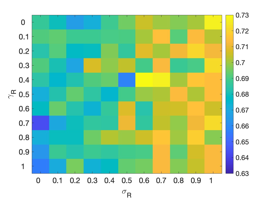
(c) case 3 ($\alpha_{S}=0.2,\alpha_{R}=0.0$)                             (d) case 4 ($\alpha_{S}=0.25,\alpha_{R}=-0.5$)

Figure 6: Survival probability with respect to $\gamma_{R}$ and $\sigma_{R}$ in PC3 (a), DU145 (b), and two other interaction cases (c-d). The survival probability is sensitive to $\sigma_{R}$, but not to $\gamma_{R}$. It implies that the birth versus death regulation of interspecies interactions impacts the survival probability more than the intraspecies competition term.

We further study the survival probability of the four interspecies interaction types–competitive ($\alpha_{S}=0.5,\alpha_{R}=0.5$), antagonistic ($\alpha_{S}=-0.5,\alpha_{R}=0.5$ and $\alpha_{S}=0.5,\alpha_{R}=-0.5$), and mutualistic ($\alpha_{S}=-0.5,\alpha_{R}=-0.5$). The parameters other than $\alpha_{i}$ are chosen to be the same as PC3.

We again confirm that the correlation of survival probability and $\sigma_{R}$ switches depending on the sign of $\alpha_{R}$. When $\alpha_{R}=0.5>0$ (competitive interactions and when S antagonizes R), the survival probability increases as $\sigma_{R}$ increases (that is, the survival probability is higher when the interaction regulates the birth process rather than the death process). However, when $\alpha_{R}=-0.5<0$ (when R antagonizes S and mutualistic interactions), the survival probability decreases as $\sigma_{R}$ increases, so the survival probability is higher when the interaction regulates the death process rather than the birth process. The value of $\sigma_{S}$ does not affect the survival probability of the resistant population.

Since the regulation of interspecies interaction affects the survival probability more than the intraspecies competition, for fixed $\alpha_{R}$, we compute the summary statistics across $\sigma_{R}$ for a fixed $\gamma_{R}$. Figure 7 shows the boxplot of the survival probabilities with respect to $\sigma_{R}$ for different interaction types.

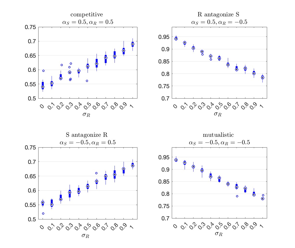
Figure 7: Survival probability with respect to $\sigma_{R}$ for different interaction regimes, including competitive, mutualistic, and antagonistic interactions ($\alpha_{S}=\pm 0.5,=\alpha_{R}=\pm 0.5$). When $\alpha_{R}=0.5$, the sensitive cells negatively impact the resistant cells, so the survival probability increases as $\sigma_{R}$ increases. When $\alpha_{R}=-0.5$, the sensitive cells positively impact the resistant cells, so the survival probability decreases as $\sigma_{R}$ increases.

The change in the survival probability of the resistant population across different values of $\sigma_{R}$ depends on the sign of $\alpha_{R}$ but not on the sign of $\alpha_{S}$. It is reasonable that the parameter that describes how the sensitive cells impact the resistant cells affects the survival probability of resistant population more than the type of interaction in the opposite direction. When $\alpha_{R}=0.5$ and the resistant cells compete with the sensitives cells, the survival probability is around $0.55$ to $0.7$. However, when $\alpha_{R}=-0.5$ and the sensitives cells positively impact the resistant cells, the survival probability increases to the level of $0.75$ to $0.95$. In addition to the numerical probability of survival, we again confirm that the correlation of $\sigma_{R}$ to the survival probability changes depending on the sign of $\alpha_{R}$. When $\alpha_{R}>0$, the survival probability increases as $\sigma_{R}$ increases, but when $\alpha_{R}<0$, the survival probability decreases as $\sigma_{R}$ increases.

5 Conclusions and Discussion

We introduced an inference method for disambiguating the birth and the death rate in a general birth-death process with $n$ distinguishable subtypes. The method requires several different time series of the counts of each subpopulation over time. This inference method was justified mathematically and the order of the error was discussed as a function of the number of time series, the size of the time step $\Delta t$, and the grid size $\Delta x$. We then demonstrated this inference method in the context of the Lokta-Volterra birth-death process. In this example, we pair the inference method for disambiguating birth and death with a sequential $\ell_{2}$-minimization inference technique to infer the parameters in the birth and death rate functions. In this case, we are able to identify all parameters through the combination of these methods. The identifiability of the birth and death rates was a result of the underlying stochasticity in the process.

In the Lokta-Voterra model, we see several notable impacts on the way the subpopulations evolve when changing how the intraspecies and interspecies interactions affect the birth and death rates. Moving the intraspecies competition to the birth rate decreases the range of the population sizes seen after a long enough period of time. Changing the interspecies interaction from the birth rate to the death rate does not have as big of an impact on the final subpopulation sizes. This is true for both the PC3 and the DU145 cell line parameter values. The placement of the interspecies interaction in the birth versus the death rate has a much bigger impact on the survival probability of the resistant population. The type of interaction determines whether the survival probability increases or decreases as the interspecies interaction moves from the death rate to the birth rate. The intraspecies competition has less of an impact on the survival probability. This is likely because when the resistant subpopulation size is small and therefore has a reasonable chance of extinction, the size of the intraspecies term is dwarfed by the size of the interspecies interaction term. Once the resistant population has grown to a size where the intraspecies term is comparable to the interspecies term, the probability of the population going extinct is small enough to be negligible on the time scale of the calculations.

There are several open questions and extensions which remain related to expansion of the theory and advancing the applications. In terms of the theory, the accuracy of the method presented here relies on data collected with a small $\Delta t$ time step between data points. This is realistic for in-silico data and even for some in-vitro data sources but is unrealistic for in-vivo studies. Expanding the method to be accurate for large $\Delta t$ time steps will require additional insights. Additionally, the method proposed here requires that the subtypes be able to be counted separately, but it is of interest to consider a way to relax this condition so that inference is possible in systems where the subtypes are indistinguishable. This would allow for broader application of the method. A limitation of our work is that we do not consider spatial effects in the population interactions, and future work includes incorporating the birth-death inference step into a spatial model. The applications of the technique would be more involved because of the additional variables to consider, such as spatial interaction and spatially correlated noise in the data. Considering phenotype switching in combination with interactions is another future direction. We also propose to consider different inference strategies for the Lotka-Volterra model parameters, such as inferring all model parameters at once [26] instead of sequentially, with an aim to understand the difference in the inference error in these situations.

One of the first applications of this method would be to consider the addition of drug effects to the model. One could consider the question of which dosing regimes are optimal based on how the subpopulation interactions are occurring (birth versus death) and how the drug is impacting the subpopulations (birth versus death). Applying the method to in-vitro data sets is another step which would further validate the method and expand the systems to which the inference method can be applied.

Declarations

• Conflict of interest/Competing interests: The authors declare that they have no known competing financial interests or personal relationships that could have appeared to influence the work reported in this paper.

• Data availability: There is no experimental or clinical data. Simulated data can be reproduced using the code below.

• Code availability: Code can be found at https://github.com/lhuynhm/inference_stochastics_interactionshetero_birthdeath

Appendix A Approximation Validation

In Section 3.1, to determine $\lambda_{k},\mu_{k}$ for each of the $N_{k}$ subpopulations, we make the approximation that $\Delta^{+}N_{k}|{\bm{N}}(t)$ is binomial with parameters $n=N_{k}(t)$ and $p=\lambda_{k}N_{k}(t)^{-1}\Delta t$ and $\Delta^{-}N_{k}|{\bm{N}}(t)$ is Binomial$(N_{k}(t),\mu_{k}N_{k}(t)^{-1}\Delta t)$. We then discard error of size $o(\Delta t)$, and in particular, we ignore the covariance between the number of birth and numbers of deaths in a time interval.

Claim: The covariance between $\Delta^{+}N_{k}(t),\Delta^{-}N_{k}(t)$ is $O(\Delta t^{2})=o(\Delta t)$.

Proof.

We want to understand, through an approximation, the branching behavior of a population of individuals over the time interval $[t,t+\Delta t)$ for $\Delta t$ small, where each individual alive splits into two and dies independently at an exponential time with rate $\lambda_{k}$ and rate $\mu_{k}$, respectively.

We write an approximation of the behavior where we ignore error of size $o(\Delta t)$, using the following assumptions.

1. Individuals alive at time $t$ have at most one event during the time interval. That is, an individual either dies or splits - not both. The probability of multiple exponential events during a $\Delta t$ time interval is $O(\Delta t^{2})$, so this assumption is exact up to error of size $o(\Delta t)$.

2. The probability of an individual having one birth event during the time interval is $\lambda_{k}\Delta t+O(\Delta t^{2})$. The probability of an individual having one death event during the interval is $\mu_{k}\Delta t+O(\Delta t^{2})$. The probability of no events (neither birth nor death) is $1-(\lambda_{k}+\mu_{k})\Delta t+O(\Delta t^{2})$. These probabilities come directly from Taylor expansions of the exponential and from the calculation that the probability of two or more events is $O(\Delta t^{2})$.

3. Individuals born during the interval $(t,t+\Delta t)$ do not branch or die. Again, this is justified by the fact that two or more events, specifically the birth event of a new individual and then that new individual splitting or dying, happens with probability $O(\Delta t)^{2}$, and therefore these events are small enough to ignore.

With these assumptions, a conditional covariance calculation can be made for the two binomials.

$$\operatorname{Cov}(\Delta^{+}N_{k}(t), \Delta^{-}N_{k}(t)|{\bm{N}}(t))$$

$$=\mathbb{E}[\Delta^{+}N_{k}(t)\Delta^{-}N_{k}(t)|{\bm{N}}(t)]-\mathbb{E}[\Delta^{+}N_{k}(t)|{\bm{N}}(t)]\mathbb{E}[\Delta^{-}N_{k}(t)|{\bm{N}}(t)]$$

$$=\mathbb{E}[\Delta^{+}N_{k}(t)\Delta^{-}N_{k}(t)|{\bm{N}}(t)]-(\lambda_{k}\Delta t)(\mu_{k}\Delta t)$$

$$=\mathbb{E}[\Delta^{+}N_{k}(t)\mathbb{E}[\Delta^{-}N_{k}(t)|\Delta^{+}N_{k}(t),{\bm{N}}(t)]|{\bm{N}}(t)]-(\Delta t)^{2}\lambda_{k}\mu_{k}.$$ (41)

Notice that by the assumptions above,

$$\Delta^{-}N_{k}(t)|\Delta^{+}N_{k}(t),{\bm{N}}(t)\overset{d}{=}\operatorname{Bin}(N_{k}(t)-\Delta^{+}N_{k}(t),\mu_{k}N_{k}(t)^{-1}\Delta t)$$ (42)

and so

$$\mathbb{E}[\Delta^{-}N_{k}(t)|\Delta^{+}N_{k}(t),{\bm{N}}(t)]=(N_{k}(t)-\Delta^{+}N_{k}(t))\mu_{k}N_{k}(t)^{-1}\Delta t.$$ (43)

Plugging this back in to the covariance calculation, we get

$$\operatorname{Cov}(\Delta^{+}N_{k}(t), \Delta^{-}N_{k}(t)|{\bm{N}}(t))$$

$$=\mathbb{E}[\Delta^{+}N_{k}(t)(N_{k}(t)-\Delta^{+}N_{k}(t))\mu_{k}N_{k}(t)^{-1}\Delta t]-(\Delta t)^{2}\lambda_{k}\mu_{k}$$

$$=N_{k}(t)\mu\Delta t\mathbb{E}[\Delta^{+}N_{k}(t)]-\mu\Delta t\mathbb{E}[\Delta^{+}N_{k}(t)^{2}]-N_{k}(t)^{2}(\Delta t)^{2}\lambda\mu$$

$$=N_{k}(t)^{2}\mu\lambda(\Delta t)^{2}-\mu\Delta t\left(N_{k}(t)\Delta t\lambda(1-\Delta t\lambda)+N_{k}(t)^{2}\lambda^{2}(\Delta t)^{2}\right)$$

$$\hskip 10.00002pt-N_{k}(t)^{2}(\Delta t)^{2}\lambda\mu.$$

It is clear that this is $O(\Delta t^{2})$, as claimed. ∎

Claim: If we approximate $\Delta^{+}N_{k}|{\bm{N}}(t)$ and $\Delta^{-}N_{k}|{\bm{N}}(t)$ by Poisson random variables with parameter $\lambda_{k}\Delta t$ and $\mu_{k}\Delta t$, respectively, then we get the same equations for $\lambda_{k},\mu_{k}$ up to $o(\Delta t)$.

Proof.

Note here that the parameters are chosen such that the mean of the Poisson approximation equals the mean of the binomial approximation described above. So all that remains is to check that the variances are equal up to $o(\Delta t)$.

If $X$ is a Poisson$(np)$ random variable and $Y$ is a Binomial$(n,p)$ random variable for parameters $n,p$ with $p=O(\Delta t)$, then from the formulas for variance for each of these random variables,

$$\operatorname{Var}(X) =np$$ (44)

$$\operatorname{Var}(Y) =np(1-p)=np-np^{2}=np+O(\Delta t^{2})=np+o(\Delta t).$$ (45)

Because the parameters were chosen such that the means would be equal, the claim follows. ∎

Therefore, up to error of $o(\Delta t)$, the equations for $\lambda_{k},\mu_{k}$ are the same whether the approximation is made with a binomial or a Poisson random variable. The heuristic justification for a binomial random variable is that it “counts the number of individuals that give birth in a time period if each birth is independent”. The heuristic argument for a Poisson approximation is that a Poisson random variable counts the number of exponential events in a fixed $\Delta t$ time period, if the rate is constant (that is, if the rate of birth does not update until the end of the $\Delta t$ time interval). The validity of the approximation in both these cases relies on essentially the same thing–that in a short time period, the branch rate is essentially unchanged.

When events are exponentially distributed with rate $\lambda$, the probability of more than one event in a time interval $\Delta t$ is $O(\Delta t^{2})$. Therefore, the true distribution of $\Delta N_{k}(t)$ is up to $o(\Delta t)$ is

$$\mathbb{P}(\Delta N_{k}(t)=1|{\bm{N}}(t)) =\lambda_{k}\Delta t+o(\Delta t)$$ (46)

$$\mathbb{P}(\Delta N_{k}(t)=-1|{\bm{N}}(t)) =\mu_{k}\Delta t+o(\Delta t)$$ (47)

$$\mathbb{P}(\Delta N_{k}(t)=0|{\bm{N}}(t)) =e^{-(\lambda_{k}+\mu_{k})\Delta t}=1-(\lambda_{k}+\mu_{k})\Delta t+o(\Delta t).$$ (48)

Claim: The equations for $\lambda_{k}$ and $\mu_{k}$ are accurate up to $o(\Delta t)$.

Proof.

We can compute the mean and variance of the random variable with this distribution to be

$$\mathbb{E}[\Delta N_{k}(t)] =\lambda_{k}\Delta t-\mu_{k}\Delta t+o(\Delta t^{2})$$ (49)

$$\operatorname{Var}(\Delta N_{k}(t)) =\lambda_{k}\Delta t+\mu_{k}\Delta t+o(\Delta t^{2}).$$ (50)

These equations are the same up to $o(\Delta t)$ and therefore result in the same equations for $\lambda_{k},\mu_{k}$. ∎

This shows that the approximation we use is in fact correct up to $o(\Delta t)$. Moving past this order would require more careful justification.

Appendix B Reference for Parameters

Parameter	PC3 Cell line	DU145 Cell line	Reference
$r_{S}$	0.293	0.306	[16]∗
$K_{S}$	843	724	[16]∗
$\delta_{S}$	0.3784	0.3784	[16]∗
$r_{R}$	0.363	0.21	[16]∗
$K_{R}$	2217	1388	[16]∗
$\delta_{R}$	0.3396	0.3396	[16]∗
$\alpha_{S}$	0.0	$-0.5$	[16]∗
$\alpha_{R}$	0.2	0.25	[16]∗
$\gamma_{S}$	[0,1]	[0,1]	$\star$
$\gamma_{R}$	[0,1]	[0,1]	$\star$
$\sigma_{S}$	[0,1]	[0,1]	$\star$
$\sigma_{R}$	[0,1]	[0,1]	$\star$

Table 6: Model parameters of prostate cancer cell lines, PC3 and DU145, their values and references. Most of the Lotka-Volterra model parameters are directly from [16]. The parameters with [16]^∗: the values recalculated from the cellular automata model developed in [16] to match the experimental data. The birth and death weight parameters with $\star$: the values are studied in this paper.

References

- \bibcommenthead
- Vermeij [1994] Vermeij, G.J.: The evolutionary interaction among species: selection, escalation, and coevolution. Annual review of ecology and systematics, 219–236 (1994)
- Pelletier et al. [2009] Pelletier, F., Garant, D., Hendry, A.P.: Eco-evolutionary dynamics. The Royal Society London (2009)
- Meacham and Morrison [2013] Meacham, C.E., Morrison, S.J.: Tumour heterogeneity and cancer cell plasticity. Nature 501(7467), 328–337 (2013)
- Dagogo-Jack and Shaw [2018] Dagogo-Jack, I., Shaw, A.T.: Tumour heterogeneity and resistance to cancer therapies. Nature reviews Clinical oncology 15(2), 81–94 (2018)
- Turajlic et al. [2019] Turajlic, S., Sottoriva, A., Graham, T., Swanton, C.: Resolving genetic heterogeneity in cancer. Nature Reviews Genetics 20(7), 404–416 (2019)
- Gefen and Balaban [2009] Gefen, O., Balaban, N.Q.: The importance of being persistent: heterogeneity of bacterial populations under antibiotic stress. FEMS microbiology reviews 33(4), 704–717 (2009)
- Dewachter et al. [2019] Dewachter, L., Fauvart, M., Michiels, J.: Bacterial heterogeneity and antibiotic survival: understanding and combatting persistence and heteroresistance. Molecular cell 76(2), 255–267 (2019)
- Kauffman et al. [2007] Kauffman, M.J., Varley, N., Smith, D.W., Stahler, D.R., MacNulty, D.R., Boyce, M.S.: Landscape heterogeneity shapes predation in a newly restored predator–prey system. Ecology letters 10(8), 690–700 (2007)
- Stover et al. [2012] Stover, J.P., Kendall, B.E., Fox, G.A.: Demographic heterogeneity impacts density-dependent population dynamics. Theoretical Ecology 5, 297–309 (2012)
- Aguadé-Gorgorió et al. [2024] Aguadé-Gorgorió, G., Anderson, A.R., Solé, R.: Modeling tumors as complex ecosystems. iScience (2024)
- Ogbunugafor and Eppstein [2016] Ogbunugafor, C.B., Eppstein, M.J.: Competition along trajectories governs adaptation rates towards antimicrobial resistance. Nature ecology & evolution 1(1), 0007 (2016)
- De Wit et al. [2022] De Wit, G., Svet, L., Lories, B., Steenackers, H.P.: Microbial interspecies interactions and their impact on the emergence and spread of antimicrobial resistance. Annual Review of Microbiology 76(1), 179–192 (2022)
- Nanayakkara et al. [2021] Nanayakkara, A.K., Boucher, H.W., Fowler Jr, V.G., Jezek, A., Outterson, K., Greenberg, D.E.: Antibiotic resistance in the patient with cancer: Escalating challenges and paths forward. CA: a cancer journal for clinicians 71(6), 488–504 (2021)
- Fair and Tor [2014] Fair, R.J., Tor, Y.: Antibiotics and bacterial resistance in the 21st century. Perspectives in medicinal chemistry 6, 14459 (2014)
- Czuppon et al. [2023] Czuppon, P., Day, T., Débarre, F., Blanquart, F.: A stochastic analysis of the interplay between antibiotic dose, mode of action, and bacterial competition in the evolution of antibiotic resistance. PLoS Computational Biology 19(8), 1011364 (2023)
- Paczkowski et al. [2021] Paczkowski, M., Kretzschmar, W.W., Markelc, B., Liu, S.K., Kunz-Schughart, L.A., Harris, A.L., Partridge, M., Byrne, H.M., Kannan, P.: Reciprocal interactions between tumour cell populations enhance growth and reduce radiation sensitivity in prostate cancer. Communications Biology 4(1), 6 (2021)
- Maltas et al. [2024] Maltas, J., Tadele, D.S., Durmaz, A., McFarland, C.D., Hinczewski, M., Scott, J.G.: Frequency-dependent ecological interactions increase the prevalence, and shape the distribution, of preexisting drug resistance. PRX Life 2(2), 023010 (2024)
- Huynh et al. [2023] Huynh, L., Scott, J.G., Thomas, P.J.: Inferring density-dependent population dynamics mechanisms through rate disambiguation for logistic birth-death processes. Journal of Mathematical Biology 86(4), 50 (2023)
- Lee et al. [2023] Lee, N.D., Kaveh, K., Bozic, I.: Clonal interactions in cancer: Integrating quantitative models with experimental and clinical data. In: Seminars in Cancer Biology, vol. 92, pp. 61–73 (2023). Elsevier
- Pankey and Sabath [2004] Pankey, G.A., Sabath, L.: Clinical relevance of bacteriostatic versus bactericidal mechanisms of action in the treatment of gram-positive bacterial infections. Clinical infectious diseases 38(6), 864–870 (2004)
- Hanahan and Weinberg [2011] Hanahan, D., Weinberg, R.A.: Hallmarks of cancer: the next generation. cell 144(5), 646–674 (2011)
- Fouad and Aanei [2017] Fouad, Y.A., Aanei, C.: Revisiting the hallmarks of cancer. American journal of cancer research 7(5), 1016 (2017)
- Browning et al. [2020] Browning, A.P., Warne, D.J., Burrage, K., Baker, R.E., Simpson, M.J.: Identifiability analysis for stochastic differential equation models in systems biology. Journal of the Royal Society Interface 17(173), 20200652 (2020)
- Remien and Ridenhour [2021] Remien, C.H., Ridenhour, B.J.: Structural identifiability of the generalized lotka-volterra model for microbiome studies. Royal Society Open Science 8 (2021) https://doi.org/10.1098/rsos.201378
- Greene et al. [2019] Greene, J.M., Gevertz, J.L., Sontag, E.D.: Mathematical approach to differentiate spontaneous and induced evolution to drug resistance during cancer treatment. JCO Clinical Cancer Informatics (2019) https://doi.org/10.1200/CCI.18.00087
- Cho et al. [2023] Cho, H., Lewis, A.L., Storey, K.M., Byrne, H.M.: Designing experimental conditions to use the lotka–volterra model to infer tumor cell line interaction types. Journal of Theoretical Biology 559, 111377 (2023)
- Crawford et al. [2014] Crawford, F.W., Minin, V.N., Suchard, M.A.: Estimation for general birth-death processes. Journal of the American Statistical Association 109(506), 730–747 (2014)
- Gunnarsson et al. [2023] Gunnarsson, E.B., Foo, J., Leder, K.: Statistical inference of the rates of cell proliferation and phenotypic switching in cancer. Journal of Theoretical Biology 568, 111497 (2023)
- Emond et al. [2023] Emond, R., Griffiths, J.I., Grolmusz, V.K., Nath, A., Chen, J., Medina, E.F., Sousa, R.S., Synold, T., Adler, F.R., Bild, A.H.: Cell facilitation promotes growth and survival under drug pressure in breast cancer. Nature Communications 14(1), 3851 (2023)
- Maltas et al. [2024] Maltas, J., Killarney, S.T., Singleton, K.R., Strobl, M.A., Washart, R., Wood, K.C., Wood, K.B.: Drug dependence in cancer is exploitable by optimally constructed treatment holidays. Nature ecology & evolution 8(1), 147–162 (2024)
- Haario et al. [2006] Haario, H., Laine, M., Mira, A., Saksman, E.: DRAM: Efficient adaptive MCMC. Statistics and Computing 16(4), 339–354 (2006) https://doi.org/%****␣main_journal_submission.bbl␣Line␣525␣****10.1007/s11222-006-9438-0