WaveDiffusion: Exploring Full Waveform Inversion via Joint Diffusion in the Latent Space

Abstract

Full Waveform Inversion (FWI) is a vital technique for reconstructing high-resolution subsurface velocity maps from seismic waveform data, governed by partial differential equations (PDEs) that model wave propagation. Traditional machine learning approaches typically map seismic data to velocity maps by encoding seismic waveforms into latent embeddings and decoding them into velocity maps. In this paper, we introduce a novel framework that reframes FWI as a joint diffusion process in a shared latent space, bridging seismic waveform data and velocity maps. Our approach has two key components: first, we merge the bottlenecks of two separate autoencoders—one for seismic data and one for velocity maps—into a unified latent space using vector quantization to establish a shared codebook. Second, we train a diffusion model in this latent space, enabling the simultaneous generation of seismic and velocity map pairs by sampling and denoising the latent representations, followed by decoding each modality with its respective decoder. Remarkably, our jointly generated seismic-velocity pairs approximately satisfy the governing PDE without any additional constraint, offering a new geometric interpretation of FWI. The diffusion process learns to score the latent space according to its deviation from the PDE, with higher scores representing smaller deviations from the true solutions. By following this diffusion process, the model traces a path from random initialization to a valid solution of the governing PDE. Our experiments on the OpenFWI dataset demonstrate that the generated seismic and velocity map pairs not only exhibit high fidelity and diversity but also adhere to the physical constraints imposed by the governing PDE.

1 Introduction

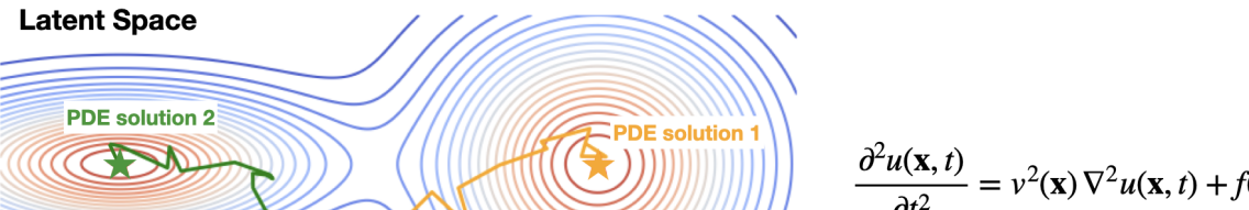
Figure 1: Overview of WaveDiffusion. WaveDiffusion refines the solution space of the governing wave equation by a diffusion process. Each peak (colored stars) corresponds to a PDE solution. The diffusion process transforms latent points in non-solution regions (gray squares) in the valleys toward accurate solutions consistent with the governing PDE.

Subsurface imaging is crucial for addressing many scientific and industrial challenges, such as understanding global earthquakes [1, 2], monitoring greenhouse gas storage [3, 4], improving ultrasound medical imaging [5, 6], and aiding oil and gas exploration [7, 8]. Subsurface structure is typically represented by acoustic wave velocity, which can be inferred from seismic data due to the physical relationship between them governed by a partial differential equation (PDE)—specifically, the acoustic wave equation [9, 10]. Full waveform inversion (FWI) is a powerful technique for reconstructing high-resolution subsurface acoustic velocity maps from seismic data. It is framed as a non-linear optimization problem: given seismic data $s$, the task is to solve for the velocity map $v$ according to the governing wave equation [11, 12].

Recently, machine learning-based approaches have been introduced to solve FWI [13, 14, 15, 16]. These methods typically use neural networks, particularly encoder-decoder architectures, to directly map seismic data to subsurface velocity maps, treating the FWI task as an image-to-image translation problem [17, 18, 19]. A more recent approach introduced generative diffusion models to regularize FWI by generating prior distributions for plausible velocity models, which guide the inversion process [20]. This approach treats FWI as a conditional generation problem, i.e. generating velocity maps using seismic data as condition.

In this paper, we explore a new direction by considering FWI as a joint generative process. In contrast to prior works that treat FWI as a conditional generation problem (where the velocity map is generated for a given seismic waveform), we are curious whether the two modalities—seismic waveform data and velocity map—can be generated simultaneously from a common latent space. Interestingly, we discovered that not only can these two modalities be jointly generated, but the generated seismic data and velocity maps also naturally satisfy the governing PDE without requiring any additional constraints. To achieve this, we propose a method with two key steps: first, we introduce a dual autoencoder architecture where both seismic data and velocity maps are encoded into a shared latent space, capturing the essential relationships between the two modalities. This shared latent space provides a coarse approximation of the wave equation solution space. Second, we apply a diffusion process in their common latent space, progressively refining the latent representations from random initializations. The corresponding decoders then generate seismic data and velocity maps from the refined latent representations. Our experiments on the OpenFWI dataset [15] empirically confirm that the jointly generated pairs satisfy the governing PDE.

This approach provides a new perspective on solving the governing wave equation. Unlike traditional FWI, which solves for one modality given the other, our method demonstrates that both seismic data and velocity maps can be solved simultaneously. This is achieved through a diffusion process within a shared latent space. Each point in this space corresponds to a seismic-velocity pair (after decoding), though not all points inherently satisfy the governing PDE. The diffusion model, however, learns to score each point based on its deviation from the PDE. By following the iterative denoising process, we trace a path from random initialization (with a lower score) to a valid solution (with a higher score) that satisfies both modalities of the PDE, as shown in Figure 1. With each denoising step, the deviation from the PDE decreases, leading to a more accurate solution.

It’s important to note that our goal is not to push the boundaries of FWI performance but to offer a new perspective by extending FWI from a conditional generation problem to a joint generation problem. We hope that this approach will inspire deeper exploration and understanding within the research community, paving the way for new insights in computational imaging.

2 FWI Overview

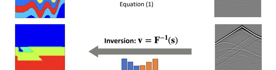
Figure 2: Illustration of data-driven FWI: forward simulation of seismic data $s$ via PDE $\mathbf{F}$ and inversion of $v$ via neural networks.

Full Waveform Inversion (FWI) is a crucial technique for constructing high-resolution velocity maps of the subsurface from seismic data. The fundamental goal of FWI is to recover the velocity model $v(\mathbf{x})$ that governs the propagation of seismic waves, using observed seismic data $s(\mathbf{x_{r}},t)$.

FWI is traditionally framed as an iterative optimization problem, where synthetic seismic data is generated through forward modeling and compared against observed data to update the velocity model iteratively. The synthetic data is typically computed by solving a partial differential equation (PDE) known as the wave equation. For the acoustic wave equation, this can be expressed as:

$$\frac{\partial^{2}u(\mathbf{x},t)}{\partial t^{2}}=v^{2}(\mathbf{x})\nabla^{2}u(\mathbf{x},t)+f(\mathbf{x_{s}},t)$$ (1)

where $u(\mathbf{x},t)$ represents the seismic wavefield, $v(\mathbf{x})$ is the subsurface velocity, $\nabla^{2}$ is the Laplacian operator, and $f(\mathbf{x_{s}},t)$ is the source term. The objective of FWI is to minimize the misfit between observed seismic data $s_{\text{obs}}$ and synthetic data $s_{\text{syn}}$, generated by solving the wave equation. The typical data misfit objective function is:

$$\mathcal{L}_{\text{FWI}}(v)=\frac{1}{2}\sum_{t=1}^{T}\left\|s_{\text{obs}}(\mathbf{x_{r}},t)-s_{\text{syn}}(\mathbf{x_{r}},t;v)\right\|^{2}$$ (2)

where $s_{\text{obs}}$ and $s_{\text{syn}}$ represent the observed and synthetic seismic data at receiver locations $\mathbf{x_{r}}$, respectively. The optimization process involves calculating the gradient of this loss function with respect to the velocity model using methods like the adjoint state method [21]. However, this iterative process is computationally expensive and often suffers from issues related to non-linearity and non-uniqueness in the inversion problem.

Recent advances in machine learning have introduced data-driven approaches for solving the FWI problem. These methods avoid the need for iterative PDE solvers by training neural networks to map seismic data directly to velocity maps. Approaches like InversionNet [13] treat the FWI problem as an image-to-image translation task, where convolutional encoder-decoder architectures are employed to generate velocity maps from seismic data in a single forward pass. This dramatically reduces computational costs compared to traditional methods.

However, while these machine learning-based models provide computational efficiency, they lack the physical grounding of traditional methods and often consider FWI as a conditional generation problem. As a result, they do not guarantee that the generated velocity maps satisfy the governing wave equation, potentially leading to physically inconsistent solutions.

3 WaveDiffusion: Our Method

In this section, we introduce WaveDiffusion, an extension of FWI that moves beyond solving for velocity given seismic data, enabling the simultaneous solution of both modalities. Our approach involves two key steps: (1) a dual autoencoder architecture with vector quantization that maps seismic data and velocity maps into a common latent space, and (2) a diffusion model applied in this common latent space, followed by two decoders that generate both modalities simultaneously. This method provides a new perspective on addressing the underlying PDE.

3.1 Motivation for Joint Generation

Existing machine learning-based approaches typically focus on translating one modality (seismic data) into another (velocity map) using encoder-decoder architectures. Mathematically, these methods provide only a partial solution to the governing PDE, as they rely on the availability of one modality. In contrast, our method tackles the more challenging problem: can both modalities be solved simultaneously?

Inspired by the success of diffusion models in generating multimodal outputs, such as images, audio, and video, we demonstrate that the joint distribution of seismic data and velocity maps can be modeled using a diffusion framework. This allows the two modalities to be generated simultaneously. Following the structure of latent diffusion models [22], our approach involves two main steps: (1) a dual autoencoder with vector quantization and (2) a joint diffusion process for refining the latent representations.

3.2 Dual Autoencoder with Vector Quantization

Figure 3: Dual autoencoder architecture: VQDAE has two branches of encoders-decoders. The blue "VQ" block is the vector quantization layer. The orange block $z$ is the common latent space shared by seismic data and velocity maps, representing the coarse solution space of the PDE.

Shared Latent Space: The first step in the WaveDiffusion framework involves generating a coarse approximation to the PDE solutions using a VQDAE architecture. As shown in Figure 3, the architecture has two parallel encoder-decoder branches, where one is responsible for encoding seismic data and the other for velocity maps. The encoders map the input data into their latent vectors, which are then combined into a shared latent space $z$ using CNN layers. This shared latent space captures the essential relationships between the two modalities and ensures that the generated seismic-velocity pairs are modeled jointly, preserving their dependencies.

Vector Quantization: The vector quantization layer ensures a compact and discrete representation of the latent space. Vector quantization discretizes the continuous latent vectors, enabling the model to capture more structured patterns and long-range dependencies between the two modalities. This step is crucial for ensuring that the latent space contains representative and interpretable features, which are then refined by a diffusion process. The sample outputs from this common latent space generate plausible seismic data and velocity maps, though these pairs are coarse approximations and do not yet fully satisfy the wave equation. The joint diffusion process is then introduced to refine this latent space representation further.

3.3 Joint Diffusion Process

Figure 4: Joint Diffusion architecture: Gaussian noise is gradually added to the shared latent space $z$ for $t$ steps in the forward stage and progressively removed in the backward stage until the seismic-velocity pairs are consistent with the wave equation.

Latent Diffusion: The joint diffusion process refines the coarse approximations produced by the VQDAE model by operating on the shared latent space $z$ of the two modalities. Gaussian noise is added during the forward process, progressively perturbing the latent vector. During the backward process, the noise is removed, guiding the model toward physically valid solutions (Figure 4). This iterative refinement ensures that the generated seismic-velocity pairs satisfy the wave equation.

1. Forward Process: Gaussian noise is added to the latent vector $z$, creating a noisy representation: $z_{t}=z+\epsilon_{t}$, where $\epsilon_{t}$ is the noise applied at step $t$.

2. Backward Process: The noisy latent vector is progressively denoised through $z_{t-1}=\mathcal{L}(z_{t})$. Each backward step removes noise and refines the latent vector toward a valid solution that satisfies the wave equation.

Sampling New Solutions: After learning the backward denoising steps, new seismic-velocity pairs can be generated that satisfy the wave equation by sampling latent vectors from a Gaussian distribution and refining them using the learned backward steps.

1. Sample a latent vector $z_{t}$ from a standard Gaussian distribution: $z_{t}\sim\mathcal{N}(0,I)$.

2. Pass $z_{t}$ through the backward denoising steps: $z_{t-1}=\mathcal{L}(z_{t}),\quad z_{t-2}=\mathcal{L}(z_{t-1}),\dots,z_{0}$.

3. Decode $z_{0}$ back into seismic data and velocity maps: $\hat{x}_{\text{s}}=\mathcal{D}_{\text{s}}(z_{0}),~{}\hat{x}_{\text{v}}=\mathcal{D}_{\text{v}}(z_{0})$.

3.4 Key Insight: From Coarse to Fine Approximation

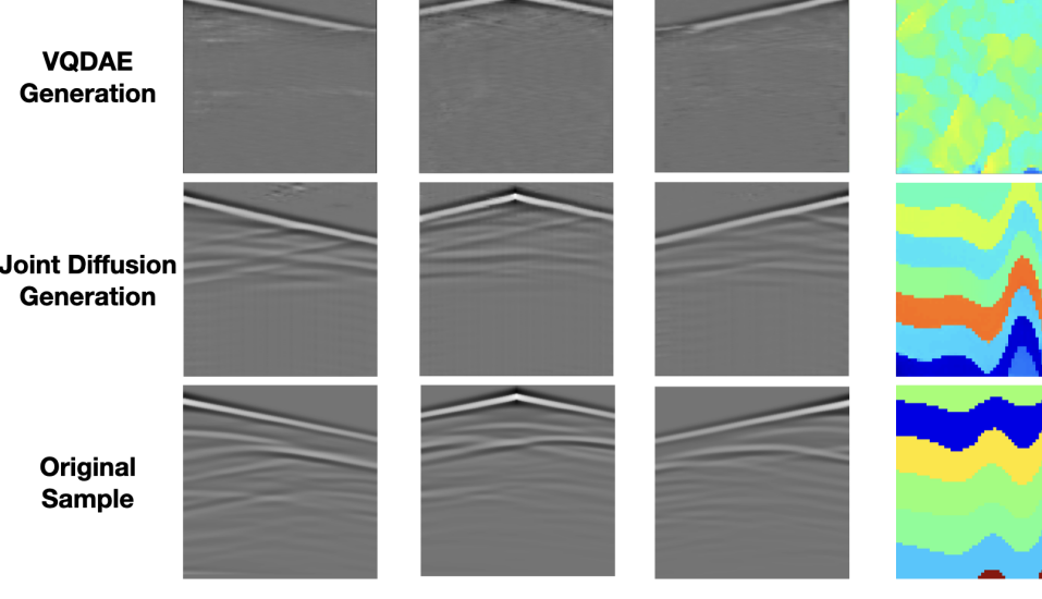
Figure 5: Comparison between generated and original samples: Examples of generated pairs by the (row 1) VQDAE and (row 2) joint diffusion. We visually compare them to (row 3) an original OpenFWI example. The VQDAE-generated samples lack the physical relationship governed by the wave equation, while the joint diffusion generation refines them to better satisfy the PDE.

Coarse and Fine Approximation Discovery: The VQDAE provides coarse approximations of the PDE solutions, producing seismic-velocity pairs that are plausible but do not fully satisfy the wave equation (Figure 5 row 1). In contrast, the joint diffusion process refines these coarse approximations into physically valid solutions (Figure 5 row 2), demonstrating that the VQDAE captures general relationships between the modalities, while the diffusion refines them to satisfy the wave equation.

Deviation Evaluation: To quantitatively assess how well the generated seismic-velocity pairs adhere to the governing wave equation, we evaluate the deviation between the generated seismic data and the synthetic ground truth seismic data simulated using a finite difference (FD) solver using the jointly generated velocity map. Specifically, we analyze the L2 distance at each forward and backward diffusion step.

In diffusion, Gaussian noise is incrementally added to the latent vector $z$ during the forward process, and progressively denoised during the backward process. For each noisy latent vector $z_{t}$ at diffusion step $t$, we decode the seismic data $\hat{x}_{\text{s}}$ and velocity map $\hat{x}_{\text{v}}$ using the respective decoders. We then simulate synthetic seismic data $x_{\text{s}}(\hat{x}_{\text{v}})$ using a finite difference operator on the decoded velocity map $\hat{x}_{\text{v}}$. The L2 distance $\|\hat{x}_{\text{s}}-x_{\text{s}}(\hat{x}_{\text{v}})\|_{2}$ measures the deviation between the generated seismic data $\hat{x}_{\text{s}}$ and the FD-simulated synthetic seismic data $x_{\text{s}}(\hat{x}_{\text{v}})$. This evaluation is repeated for every forward and backward diffusion steps to track how the deviation changes as noise is added and removed.

Figure 6: Deviation from the governing PDE. The L2 distance is calculated between (a) generated seismic data $\hat{x}_{\text{s}}$ and (b) synthetic seismic data $x_{\text{s}}(\hat{x}_{\text{v}})$ simulated from the generated velocity map using a finite difference solver.

As noise is introduced during the forward process, the generated seismic data diverges from the physically valid solutions. Conversely, during the backward diffusion process, the model removes noise, progressively reducing the L2 distance and refining the seismic-velocity pairs toward solutions that better satisfy the wave equation. The statistical evaluation of $10000$ generated pairs is shown in Figure 6, which illustrates how the deviation increases with noise in the forward process and decreases during denoising, confirming that the diffusion process scores the latent space based on how well the generated pairs adhere to the wave equation. Larger deviations from the PDE result in higher loss scores. During the backward diffusion process, these scores decrease as the generated pairs are refined into physically valid solutions (Figure 6 right).

Transforming PDE into SDE: The process of refining the latent space through diffusion can be interpreted as transforming the deterministic task of solving a PDE into a stochastic differential equation (SDE). As in [23], this SDE path allows exploration of a subspace of possible solutions, refining from coarse approximations to fine, physically consistent solutions.

4 Experiments

In this section, we present the experimental evaluation of the proposed WaveDiffusion framework. We conduct experiments on the OpenFWI dataset to evaluate the model’s performance in generating physically consistent seismic data and velocity maps. We assess the model’s FID scores, analyze its ability to generate data that adheres to the governing PDE. Then we compare the results of training the state-of-the-art models such as InversionNet using the jointly generated dataset against the original OpenFWI benchmark. We further introduce an experiment to demonstrate how the joint diffusion model compares to separately trained diffusion models in generating seismic and velocity modalities.

4.1 Dataset and Training Setup

We evaluate the performance of our WaveDiffusion framework using the OpenFWI dataset, a benchmark collection of 10 subsets of realistic synthetic seismic data paired with subsurface velocity maps, specifically designed for FWI tasks. For our experiments, we focus on three representative subsets from the full dataset:

• CurveVel_B (CVB): Subsurface structures with curved velocity layers.

• FlatVel_B (FVB): Subsurface structures with flat velocity layers.

• FlatFault_B (FFB): Flat layers intersected by faults.

We conducted two sets of training experiments:

1. Individual subset training: We trained the VQDAE and joint diffusion models separately on each of the three subsets (CVB, FVB, FFB) to evaluate their performance on individual geological structures.

2. Combined dataset training: We also trained the models on a combination of multiple datasets from OpenFWI to assess the model’s generalization capability across a wider variety of geological structures.

Network details and training hyperparameters can be found in Appendix A.1.

4.2 VQDAE and Joint Diffusion Results

4.2.1 Evaluating VQDAE Results

The VQDAE model serves as the first stage of our WaveDiffusion framework, producing coarse approximations of seismic data and velocity maps. When evaluated on the CVB subset, the VQDAE yielded an FID score of 14,207.14 for the generated velocity maps and 871.31 for the generated seismic data using an Inception-v3 model pre-trained on ImageNet [24]. Similar results were observed for the other VQDAE models trained on the remaining subsets and the combined dataset. Visualization examples are shown in Figure 5 row 1. These high FID scores suggest that the VQDAE, while generating plausible structural shapes, does not adhere closely to the true data distribution. The large disparity between seismic and velocity FID scores indicates that the generated modalities deviate more from the physical relationships governed by the wave equation as coarse approximations of the PDE solutions.

4.2.2 Joint Diffusion Results and Analysis

Table 1: FID scores for various datasets. The FID scores across the two modalities velocity maps $v$ and seismic data $s$ with different training datasets.

Metrics $\backslash$ Dataset	CVB	FVB	FFB	3 sets	10 sets
Velocity FID	186.86	357.74	447.71	612.18	733.00
Seismic FID	30.66	88.01	34.05	74.58	128.64

The joint diffusion model is used to refine the coarse VQDAE generations into physically consistent seismic-velocity pairs. We evaluated the FID scores of both modalities generated by the joint diffusion model across the three individual subsets and combined datasets. As shown in Table 1, the best performance was achieved in the CVB subset, with an FID of 186.86 for velocity and 30.66 for seismic data. As the geological complexity increases (e.g., FFB), the FID scores rise, especially for the velocity modality, indicating the challenges posed by these more complex configurations.

We further evaluated the deviation from the governing PDE by tracking FID scores during the forward diffusion and backward denoising processes (Table 2). As noise is added in the forward process, the FID scores increase significantly, peaking at 1000 timesteps (100% noise). On the other hand, as noise is progressively removed in the backward process, the FID scores decrease accordingly, reaching low values at the final step. This trend demonstrates how noise level is related to the deviation, and shows the model’s ability to refine noisy representations into physically valid solutions through the denoising process.

Table 2: FID score vs. noise level: The FID scores for the two modalities along the forward and backward diffusion processes on the CVB dataset.

Metrics $\backslash$Process	Forward: adding noise				Backward: removing noise
Noise Level (%)	0	20	50	100	100	50	20	0
Velocity FID	30.79	1135.82	3634.96	19393.46	19405.06	3569.01	620.33	186.86
Seismic FID	17.63	23.87	128.98	360.20	359.53	148.07	48.72	30.66

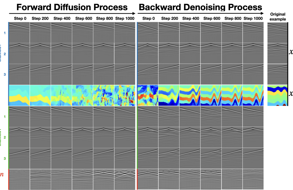
Figure 7: Visualization of deviation from PDE during diffusion: Seismic data comparison of the CVB example at different timesteps during the forward (left half) and backward diffusion processes (right half). The top three rows show seismic channels $\hat{x}_{\text{s}}$ generated by the joint diffusion model, while the fourth row shows the generated velocity map $\hat{x}_{\text{v}}$. Rows 5-7 show the synthetic seismic data $x_{\text{s}}(\hat{x}_{\text{v}})$, simulated using a finite difference PDE solver on the generated $\hat{x}_{\text{v}}$. The last row shows the deviation from the governing PDE, visualized as the channel-stacked difference between $x_{\text{s}}(\hat{x}_{\text{v}})$ and $\hat{x}_{\text{s}}$. Noise increases the deviation from the PDE during the forward diffusion, and the reverse process reduces discrepancies.

Figure 7 presents the results on the CVB dataset during the forward (adding noise) and backward (removing noise) diffusion processes. In the left half of Figure 7, during the forward diffusion process, as noise is added, the seismic data $\hat{x}_{\text{s}}$ generated by the joint diffusion model diverges more from the synthetic seismic data $x_{\text{s}}(\hat{x}_{\text{v}})$, which is simulated using the generated velocity maps $\hat{x}_{\text{v}}$. This divergence, shown as the channel-stacked difference between $x_{\text{s}}(\hat{x}_{\text{v}})$ and $\hat{x}_{\text{s}}$ in the last row, reflects the increasing deviation from the governing PDE as the noise level rises. In contrast, the right half of Figure 7 shows the backward denoising process, where noise is progressively removed, and $\hat{x}_{\text{s}}$ becomes more aligned with $x_{\text{s}}(\hat{x}_{\text{v}})$, confirming the model’s ability to refine the generated samples toward physically consistent solutions.

Similar trends can be observed in the separate FVB and FFB subset experiments and the combined datasets experiments, that in the forward diffusion, the generated modalities diverged from the ground truth, and the backward denoising converged back to PDE solutions. These results are included in the supplementary materials, further demonstrate the effectiveness of the joint diffusion model in generating realistic seismic data and velocity maps that adhere to the wave equation.

Results for the FVB and FFB single subsets can be found in Appendix A.2. Experiments with combined multiple datasets can be found in Appendix A.3.

4.2.3 Comparison with InversionNet

Table 3: Comparison of InversionNet performance across different training scenarios. Performance of three InversionNets trained with different datasets of the jointly generated and original OpenFWI data, and comparison to the benchmarks.

Dataset	Setup	RMSE	MAE	SSIM
CVB	PureGen	0.4798	0.3078	0.5204
	Gen+1%	0.3258	0.1976	0.6293
	1%Only	0.4915	0.3833	0.3625
	OpenFWI	0.2801	0.1624	0.6661
FFB	PureGen	0.2623	0.1825	0.6484
	Gen+1%	0.2396	0.1654	0.6614
	1%Only	0.3191	0.2436	0.5587
	OpenFWI	0.1723	0.1106	0.7186
FVB	PureGen	0.2766	0.1723	0.6895
	Gen+1%	0.1737	0.0893	0.8532
	1%Only	0.4045	0.2884	0.4967
	OpenFWI	0.0909	0.0417	0.9402

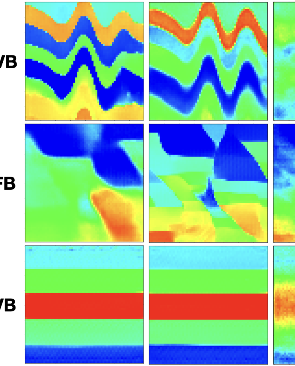
Figure 8: InversionNet performance visualization. The InversionNet predictions using the (column 1) WaveDiffusion generated samples, (column 2) WaveDiffusion generated plus 1% OpenFWI original samples, and (column 3) 1% OpenFWI original samples, compared to ground truth (column 4) across different dataset.

We conducted several experiments to evaluate the performance of InversionNet when trained on samples generated by WaveDiffusion. These experiments compare the effectiveness of generated data with the benchmarks established in the original OpenFWI paper. The following experiments were performed:

1. PureGen: Training on WaveDiffusion-generated samples and testing on the original OpenFWI dataset.

2. Gen+1%: Training on generated samples augmented with 1% of the original OpenFWI dataset and testing on the rest of the OpenFWI dataset.

3. 1%Only: Training on just 1% of the original OpenFWI dataset and testing on the rest.

The results in Table 3 summarizes the statistic metrics of these experiments, showing the performance metrics (RMSE, MAE, SSIM) for each dataset (CVB, FFB, FVB) and each training setting. Visualization comparison of the InversionNet predicted velocity maps under each setting is shown in Figure 8. Below are the key observations from these experiments:

PureGen: When InversionNet is trained on WaveDiffusion-generated samples and tested on the original OpenFWI dataset, we observe a slight drop in performance compared to the OpenFWI baseline. This indicates that although the generated samples are effective for training, they do not fully match the complexity and variability of the real data, leading to marginally lower RMSE, MAE, and SSIM values.

Gen+1%: In this experiment, where WaveDiffusion-generated samples were combined with 1% of the original OpenFWI dataset, we observe an improvement in performance compared to the PureGen setting. This shows that even a small amount of real data can significantly enhance the quality of the generated samples, allowing the model to perform closer to the OpenFWI baseline. However, the performance remains slightly below the baseline, indicating the gap between the original and generated modalities.

1%Only: Training on just 1% of the original OpenFWI dataset resulted in failure across all metrics. Both RMSE and MAE increased significantly, while SSIM dropped, showing that very limited data is insufficient for training InversionNet effectively. This emphasizes the benefit of using generated samples to supplement small datasets, as seen in the Gen+1% experiment.

These results suggest that while WaveDiffusion-generated data can be a useful supplement to real data, the addition of even a small portion of real samples greatly enhances model performance, bringing it closer to the benchmark.

4.2.4 Separate vs. Joint Diffusion

We compared the performance of our joint diffusion model against separate diffusion models, where seismic data and velocity maps were generated independently. The model architectures were kept the same, except that in the separate models, the autoencoders only had a single branch, and the latent space was no longer shared between the two modalities. Both models were trained on the CVB, FFB, and FVB datasets. The results are summarized in Table 4, while Figure 9 provides a visual comparison for the CVB dataset.

The performance, as measured by FID scores, reveals that the joint diffusion model outperforms the separate diffusion models across all datasets. For example, in the CVB subset, the joint diffusion achieves FID scores of 30.66 for seismic data and 186.86 for velocity, compared to 131.48 and 411.40, respectively, for the separate diffusion models. Similar trends are observed in the FFB and FVB datasets, where the joint diffusion consistently produces higher-quality seismic-velocity pairs.

Table 4: FID scores comparison between separate and joint generations. The FID scores comparison of the two modalities velocity maps $v$ and seismic data $s$ generated by separate diffusion models and our joint diffusion model.

Modality	Setup	CVB	FVB	FFB
Velocity	Joint	186.86	357.74	447.71
	Separate	411.40	360.90	385.32
Seismic	Joint	30.66	88.01	34.05
	Separate	131.48	179.69	117.63

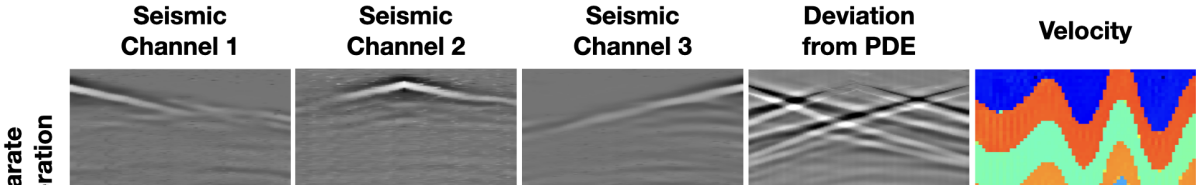
Figure 9: Visualization comparison between separate and joint generation. The comparison between the (row 1) separate generated seismic-velocity pairs using two independent diffusion models and (row 2) joint generated modalities using WaveDiffusion. The deviation from PDE is shown in column 4 as the subtraction between the generated $\hat{x_{s}}$ and the synthetic $x_{s}(\hat{x_{v}})$.

Beyond visual quality, the key distinction lies in physical consistency. While the separate diffusion models generate visually plausible outputs, especially for velocity, they do not adhere to the physical constraints of the wave equation. As shown in Figure 9, the deviation from the governing PDE is noticeable in the outputs from the separate models. In contrast, the joint diffusion model not only produces seismic-velocity pairs that are visually similar, but also ensures that these pairs satisfy the wave equation.

This comparison is visually highlighted in row 4 of Figure 9, where the deviation column illustrates the difference in physical consistency between the two approaches. While the separate diffusion models produce reasonable visual results, only the joint diffusion process generates pairs that both look realistic and meet the requirements of the governing PDE. This underscores the strength of the WaveDiffusion framework in preserving both the visual fidelity and the physical validity of the generated modalities.

5 Related works

In this section, we review three major approaches relevant to our work: traditional physics-based FWI methods, machine-learning-based FWI approaches, and the use of generative models in FWI.

5.1 Traditional Physics-based FWI

Traditional FWI methods aim to reconstruct subsurface velocity models by iteratively minimizing the difference between observed and simulated seismic data, typically using gradient-based optimization methods. The key challenge lies in solving the wave equation, which governs wave propagation through the Earth. While effective, these methods are computationally expensive and sensitive to factors such as the quality of the initial velocity model, noise in the data, and cycle-skipping issues—where the inversion algorithm converges to incorrect solutions due to poor starting models or insufficient low-frequency data [11, 7]. Techniques such as adaptive waveform inversion [12] and multiscale FWI [25] have been developed to reduce the risk of cycle-skipping and improve convergence by progressively introducing higher-frequency data. These techniques remain the treatment of FWI as a conditional generation problem using physical equations as the engine [1, 12].

5.2 Data-Driven Approaches to FWI

In recent years, machine learning approaches have been increasingly explored for FWI. Convolutional Neural Networks (CNNs) have shown promise in learning image-to-image mappings from seismic data to velocity models, bypassing the need for iterative solvers. Encoder-decoder architectures, such as those used in InversionNet [13] and VelocityGAN [26], have demonstrated the ability to predict velocity maps from seismic data while reduces computational costs by learning implicit relationships between the two modalities. Richardson’s work [17] further illustrated that deep learning models could predict velocity models efficiently. However, these approaches are still treating the FWI problem as an image-to-image translation task or a conditional generation problem [27, 20]. Recent work on neural operators [28, 29] offers a more flexible approach by learning operators that map between the two modalities in a revered direction, i.e. predicting seismic data given velocity maps. Though these neural operator methods have shown powerful capacity in mapping the two modalities, they are still constrained by their image-to-image mappings setup and cannot solve for multiple modalities simultaneously that satisfy the governing PDE.

5.3 Generative Models in FWI

Generative models, particularly Generative Adversarial Networks (GANs) and their variants, have emerged as alternatives to traditional CNN-based methods for FWI. These models aim to learn the latent representations of seismic data and velocity models, enabling the generation of synthetic training data or even direct inversion [30]. Vector Quantized Generative Adversarial Networks (VQGANs) [31], in particular, have been explored for their ability to generate high-quality modalities, such as images, audios, videos, etc. Such models can be tuned for imaging one physical modality (e.g. velocity map) given another (e.g. seismic data) [26].

Recent work has focused on Latent Diffusion Models (LDMs) [32, 33, 22], which refine latent space representations through a diffusion process. LDMs iteratively denoise latent variables, progressively improving the quality of generated samples. While these models can produce realistic-looking data, they often generate new samples of one single modality at a time. Thus, it is difficult for them to generate multiple modalities using one generative model as they lack the physical consistency to the governing PDEs that describe the relationship between these modalities. Diffusion models have been applied to FWI by Wang et al. [20], who used them to generate prior distributions for plausible velocity models as a regularization term. Their method still treats seismic data and velocity maps separately, limiting its ability to generate physically consistent seismic-velocity pairs.

6 Conclusion

In this paper, we introduced WaveDiffusion that reformulates FWI as a joint generative process of seismic-velocity pairs within a shared latent space. Unlike existing methods, which solve for one modality given the other, or treat FWI as a conditional generation problem, our method solves for both modalities simultaneously. This is achieved through a dual autoencoder architecture that encodes the two modalities into a common latent space, followed by a diffusion process that progressively refines these latent representations to adhere to the governing PDE. By following the diffusion process, the model traces a path from random initializations to valid PDE solutions, providing a new geometric interpretation of the FWI problem.

Our experiments on the OpenFWI dataset demonstrate that WaveDiffusion generates high-quality seismic-velocity pairs that not only exhibit high fidelity but also satisfy the physical constraints imposed by the wave equation. Additionally, we showed that training an existing FWI model, such as InversionNet, on WaveDiffusion-generated samples improves performance, particularly when limited amount of real data are available.

Appendix A Appendix

A.1 A. 1 Network Details and Training Hyperparameters

In this appendix section, we provide details on the network architectures and training hyperparameters used for the VQDAE and joint diffusion models in our experiments.

A.1.1 VQDAE Model

The VQDAE uses separate convolutional encoder-decoder branches that are constructed by ResNet blocks [34] for seismic and velocity data. The channel multipliers of the ResNet blocks are set to [1, 2, 2, 4, 4] for velocity maps and [1, 2, 2, 4, 4, 4, 4, 8, 8] for seismic data. The resolution for velocity maps is 64, while for seismic data it is [1024, 64]. The latent dimension $z$ is [16, 16], and the number of residual blocks is set to 3. The model was trained with a base learning rate of $4.5\times 10^{-4}$. It uses an embedding dimension of 32 and an embedding codebook size of 8192. The VQDAE employs a perceptual loss combined with a discriminator. The discriminator starts training at step 50001 with a discriminator weight of 0.5 and a perceptual weight of 0.5.

A.1.2 Joint Diffusion Model

The Joint Diffusion model is based on the LatentDiffusion architecture. The backbone network in the Joint Diffusion model is a UNet-based architecture. The UNet takes 32 input and output channels, and the model channels are set to 128. The attention resolutions are [1, 2, 4, 4], corresponding to spatial resolutions of 32, 16, 8, and 4. The model uses 2 residual blocks and channel multipliers of [1, 2, 2, 4, 4]. It also employs 8 attention heads with scale-shift normalization enabled and residual blocks that support upsampling and downsampling. The model is trained with a base learning rate of $5.0\times 10^{-5}$ and uses 1000 diffusion timesteps. The loss function applied is $L_{1}$. The diffusion process is configured with a linear noise schedule, starting from 0.0015 and ending at 0.0155.

A LambdaLinearScheduler is used to control the learning rate, with 10000 warmup steps. The initial learning rate is set to $1.0\times 10^{-6}$, which increases to a maximum of $1.0$ over the course of training.

A.1.3 Training Hyperparameters

Both the VQDAE and Joint Diffusion models were trained using the Adam optimizer, with $\beta_{1}=0.9$ and $\beta_{2}=0.999$. The models were trained with a batch size of 256 for 1000 epochs. The learning rate follows an exponential decay schedule with a decay rate of 0.98. Gradient clipping was applied with a threshold of 1.0. Early stopping was implemented when the validation loss plateaued for 10 consecutive epochs.

A.2 A. 2 FVB and FFB Results

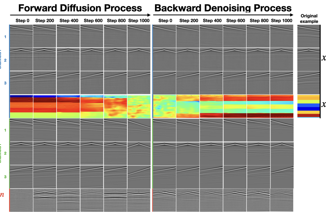
Figure 10: Visualization of deviation from PDE during diffusion on FVB: Seismic data comparison of the FVB example at different timesteps during the forward diffusion (left half) and reverse denoising processes (right half). The top three rows show seismic channels $\hat{x}_{\text{s}}$ generated by the joint diffusion model, while the fourth row shows the generated velocity map $\hat{x}_{\text{v}}$. Rows 5-7 show the synthetic seismic data $x_{\text{s}}(\hat{x}_{\text{v}})$, simulated using a finite difference PDE solver on the generated $\hat{x}_{\text{v}}$. The last row shows the deviation from the governing PDE, visualized as the channel-stacked difference between $x_{\text{s}}(\hat{x}_{\text{v}})$ and $\hat{x}_{\text{s}}$. Noise increases the deviation from the PDE during the forward diffusion, and the reverse process reduces discrepancies.

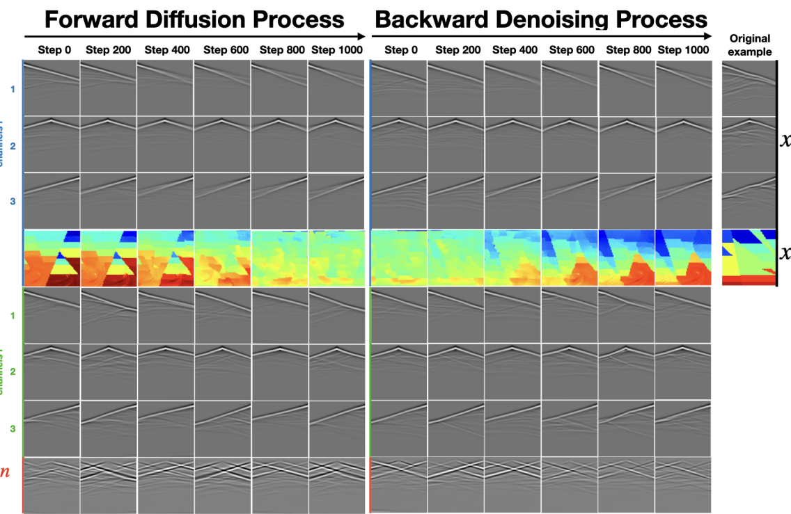
Figure 11: Visualization of deviation from PDE during diffusion on FFB: Seismic data comparison of the FFB example at different timesteps during the forward diffusion (left half) and reverse denoising processes (right half). The top three rows show seismic channels $\hat{x}_{\text{s}}$ generated by the joint diffusion model, while the fourth row shows the generated velocity map $\hat{x}_{\text{v}}$. Rows 5-7 show the synthetic seismic data $x_{\text{s}}(\hat{x}_{\text{v}})$, simulated using a finite difference PDE solver on the generated $\hat{x}_{\text{v}}$. The last row shows the deviation from the governing PDE, visualized as the channel-stacked difference between $x_{\text{s}}(\hat{x}_{\text{v}})$ and $\hat{x}_{\text{s}}$. Noise increases the deviation from the PDE during the forward diffusion, and the reverse process reduces discrepancies.

In addition to the CVB dataset, we conducted similar experiments on the FVB and FFB subsets. These subsets were chosen to evaluate the joint diffusion model’s performance in more straightforward geological scenarios—flat velocity layers and flat layers with faults.

The results from both FVB and FFB mirrored the trends observed with CVB, as shown in Figures 10 and 11, respectively. Specifically, during the forward diffusion process, the seismic data generated by the joint diffusion model increasingly diverged from the finite difference simulation data as noise was introduced. Conversely, during the reverse denoising process, the generated seismic data converged towards the “ground truth" seismic data. This consistent behavior across different geological settings further validates the effectiveness of the joint diffusion in refining the latent space to satisfy the wave equation constraints. Detailed results and visualizations for the FVB and FFB subsets are provided in the supplementary materials.

A.3 A. 3 Combined Dataset Results

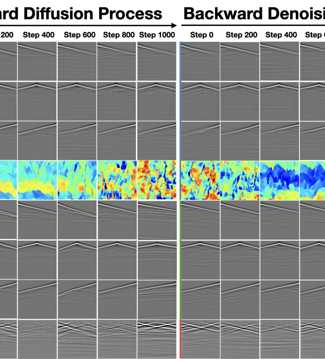
Figure 12: Visualization of deviation from PDE during diffusion on combined datasets: Seismic data comparison of the combined OpenFWI datasets example at different timesteps during the forward diffusion (left half) and reverse denoising processes (right half). The top three rows show seismic channels $\hat{x}_{\text{s}}$ generated by the joint diffusion model, while the fourth row shows the generated velocity map $\hat{x}_{\text{v}}$. Rows 5-7 show the synthetic seismic data $x_{\text{s}}(\hat{x}_{\text{v}})$, simulated using a finite difference PDE solver on the generated $\hat{x}_{\text{v}}$. The last row shows the deviation from the governing PDE, visualized as the channel-stacked difference between $x_{\text{s}}(\hat{x}_{\text{v}})$ and $\hat{x}_{\text{s}}$. Noise increases the deviation from the PDE during the forward diffusion, and the reverse process reduces discrepancies.

To assess the generalization capability of WaveDiffusion model across various geological structures, we trained the VQDAE and joint diffusion on a combined dataset that includes all the subsets.

The results on this combined dataset were consistent with those observed in the individual subsets, shown in Figure 12. The joint diffusion model effectively generated seismic data and velocity maps that adhered to the wave equation, regardless of the underlying geological configuration. The diffusion process successfully captured the shared latent space across different geological settings, though the features of different subsets are fused to some extent due to the shared latent space.

References

- [1] Jean Virieux, Amir Asnaashari, Romain Brossier, Ludovic Métivier, Alessandra Ribodetti, and Wei Zhou. An introduction to full waveform inversion. In Encyclopedia of exploration geophysics, pages R1–1. Society of Exploration Geophysicists, 2017.
- [2] Jeroen Tromp. Seismic wavefield imaging of earth’s interior across scales. Nature Reviews Earth & Environment, 1(1):40–53, 2020.
- [3] Dong Li, Suping Peng, Yinling Guo, Yongxu Lu, and Xiaoqin Cui. Co2 storage monitoring based on time-lapse seismic data via deep learning. International Journal of Greenhouse Gas Control, 108:103336, 2021.
- [4] Hanchen Wang, Yinpeng Chen, Tariq Alkhalifah, Ting Chen, Youzuo Lin, and David Alumbaugh. Default: Deep-learning based fault delineation using the ibdp passive seismic data at the decatur co2 storage site. arXiv preprint arXiv:2311.04361, 2023.
- [5] Lluís Guasch, Oscar Calderón Agudo, Meng-Xing Tang, Parashkev Nachev, and Michael Warner. Full-waveform inversion imaging of the human brain. NPJ digital medicine, 3(1):28, 2020.
- [6] Luke Lozenski, Hanchen Wang, Fu Li, Mark Anastasio, Brendt Wohlberg, Youzuo Lin, and Umberto Villa. Learned full waveform inversion incorporating task information for ultrasound computed tomography. IEEE Transactions on Computational Imaging, 2024.
- [7] Jean Virieux and Stéphane Operto. An overview of full-waveform inversion in exploration geophysics. Geophysics, 74(6):WCC1–WCC26, 2009.
- [8] Hanchen Wang and Tariq Alkhalifah. Microseismic imaging using a source function independent full waveform inversion method. Geophysical Journal International, 214(1):46–57, 2018.
- [9] Robert E Sheriff and Lloyd P Geldart. Exploration seismology. Cambridge university press, 1995.
- [10] Peter M Shearer. Introduction to seismology. Cambridge university press, 2019.
- [11] Albert Tarantola. Inversion of seismic reflection data in the acoustic approximation. Geophysics, 49(8):1259–1266, 1984.
- [12] Michael Warner and Lluís Guasch. Adaptive waveform inversion: Theory. Geophysics, 81(6):R429–R445, 2016.
- [13] Yue Wu and Youzuo Lin. Inversionnet: An efficient and accurate data-driven full waveform inversion. IEEE Transactions on Computational Imaging, 6:419–433, 2019.
- [14] Hongyu Sun and Laurent Demanet. Extrapolated full-waveform inversion with deep learning. Geophysics, 85(3):R275–R288, 2020.
- [15] Chengyuan Deng, Shihang Feng, Hanchen Wang, Xitong Zhang, Peng Jin, Yinan Feng, Qili Zeng, Yinpeng Chen, and Youzuo Lin. Openfwi: Large-scale multi-structural benchmark datasets for full waveform inversion. Advances in Neural Information Processing Systems, 35:6007–6020, 2022.
- [16] S Mostafa Mousavi and Gregory C Beroza. Deep-learning seismology. Science, 377(6607):eabm4470, 2022.
- [17] Alan Richardson. Seismic full-waveform inversion using deep learning tools and techniques. arXiv preprint arXiv:1801.07232, 2018.
- [18] Shihang Feng, Youzuo Lin, and Brendt Wohlberg. Multiscale data-driven seismic full-waveform inversion with field data study. IEEE transactions on geoscience and remote sensing, 60:1–14, 2021.
- [19] Peng Jin, Yinan Feng, Shihang Feng, Hanchen Wang, Yinpeng Chen, Benjamin Consolvo, Zicheng Liu, and Youzuo Lin. An empirical study of large-scale data-driven full waveform inversion. Scientific Reports, 14(1):20034, 2024.
- [20] Fu Wang, Xinquan Huang, and Tariq A Alkhalifah. A prior regularized full waveform inversion using generative diffusion models. IEEE Transactions on Geoscience and Remote Sensing, 61:1–11, 2023.
- [21] R-E Plessix. A review of the adjoint-state method for computing the gradient of a functional with geophysical applications. Geophysical Journal International, 167(2):495–503, 2006.
- [22] Robin Rombach, Andreas Blattmann, Dominik Lorenz, Patrick Esser, and Björn Ommer. High-resolution image synthesis with latent diffusion models. In Proceedings of the IEEE/CVF conference on computer vision and pattern recognition, pages 10684–10695, 2022.
- [23] Yang Song, Jascha Sohl-Dickstein, Diederik P Kingma, Abhishek Kumar, Stefano Ermon, and Ben Poole. Score-based generative modeling through stochastic differential equations. arXiv preprint arXiv:2011.13456, 2020.
- [24] Christian Szegedy, Vincent Vanhoucke, Sergey Ioffe, Jon Shlens, and Zbigniew Wojna. Rethinking the inception architecture for computer vision. In Proceedings of the IEEE conference on computer vision and pattern recognition, pages 2818–2826, 2016.
- [25] C Bunks, FM Saleck, S Zaleski, and G Chavent. Multiscale seismic waveform inversion. Geophysics, 60(5):1457–1473, 1995.
- [26] Zhongping Zhang, Yue Wu, Zheng Zhou, and Youzuo Lin. Velocitygan: Subsurface velocity image estimation using conditional adversarial networks. In 2019 IEEE Winter Conference on Applications of Computer Vision (WACV), pages 705–714. IEEE, 2019.
- [27] Yinhao Zhu, Nicholas Zabaras, Phaedon-Stelios Koutsourelakis, and Paris Perdikaris. Physics-constrained deep learning for high-dimensional surrogate modeling and uncertainty quantification without labeled data. Journal of Computational Physics, 394:56–81, 2019.
- [28] Zongyi Li, Nikola Kovachki, Kamyar Azizzadenesheli, Burigede Liu, Kaushik Bhattacharya, Andrew Stuart, and Anima Anandkumar. Fourier neural operator for parametric partial differential equations. arXiv preprint arXiv:2010.08895, 2020.
- [29] Bian Li, Hanchen Wang, Shihang Feng, Xiu Yang, and Youzuo Lin. Solving seismic wave equations on variable velocity models with fourier neural operator. IEEE Transactions on Geoscience and Remote Sensing, 61:1–18, 2023.
- [30] Ian Goodfellow, Jean Pouget-Abadie, Mehdi Mirza, Bing Xu, David Warde-Farley, Sherjil Ozair, Aaron Courville, and Yoshua Bengio. Generative adversarial networks. Communications of the ACM, 63(11):139–144, 2020.
- [31] Patrick Esser, Robin Rombach, and Björn Ommer. Taming transformers for high-resolution image synthesis, 2021.
- [32] Jonathan Ho, Ajay Jain, and Pieter Abbeel. Denoising diffusion probabilistic models. Advances in neural information processing systems, 33:6840–6851, 2020.
- [33] Prafulla Dhariwal and Alexander Nichol. Diffusion models beat gans on image synthesis. Advances in neural information processing systems, 34:8780–8794, 2021.
- [34] Kaiming He, Xiangyu Zhang, Shaoqing Ren, and Jian Sun. Deep residual learning for image recognition. In Proceedings of the IEEE conference on computer vision and pattern recognition, pages 770–778, 2016.