Hardness-Dependent Adiabatic Schedules
for Analog Quantum Computing

Abstract

We propose a numerical approach to design highly efficient adiabatic schedules for analog quantum computing, focusing on the maximum independent set problem and neutral atom platforms. Based on a representative dataset of small graphs, we present numerical evidences that the optimum schedules depend principally on the hardness of the problem rather than on its size. These schedules perform better than the benchmark protocols and admit a straightforward implementation in the hardware. This allows us to extrapolate the results to larger graphs and to successfully solve moderately hard problems using QuEra’s 256-qubit Aquila computer. We believe that extending our approach to hybrid algorithms could be the key to solve the hardest instances with the current technology, making yet another step toward real-world applications.

1 Introduction

In recent years, quantum computers have emerged as a promising way to solve complex optimization tasks in science and industry [1, 2, 3, 4]. Typically, the problem of interest is encoded in the ground state of a quantum Hamiltonian, which can be reached through adiabatic evolution starting from an easy-to-prepare initial state [5, 6, 7, 8]. Advanced protocols have to be developed to overcome not only the experimental limitations, such as qubit decoherence and control errors, but also the intrinsic complication of vanishing gap in the eigenspectrum during the evolution [9, 10, 11, 12].

Here, we focus on the maximum independent set (MIS) problem, where the task is to find the largest set of vertices that do not share an edge in a graph. Such problems appear naturally in practical applications, for instance while designing resilient communication networks [13], and are known to be NP-hard in general [14]. Finding a MIS is still a difficult task in the particular case of unit disk graphs [15, 16], in which vertices are connected by an edge if they are closer than a fixed distance. This family of graphs admits a direct mapping to arrays of Rydberg atoms, which explains the popularity of the MIS problem in analog quantum computing [17, 18, 19]. In that setting, optical tweezers enable arbitrary arrangements of atoms and controlled laser pulses manipulate the quantum states [20, 21]. The lasers then drive the evolution of the system according to schedules that are specific to the problem to be solved.

The precise description of the adiabatic schedules is of utmost importance since it conditions the success of the quantum algorithm. Many methods have been proposed in this regard: quantum approximate optimization algorithm and variational quantum eigensolver [22, 23, 24], shortcut to adiabadicity and counterdiabatic protocol [25, 26, 27, 28], Bayesian optimization and machine learning [29, 30], to name a few. Most aforementioned methods require multiple iterations to be run on a quantum device and to be updated by a classical optimizer and thus belong to the class of hybrid algorithms [31]. By their very nature, these algorithms cost both time and money as they make intense use of the quantum hardware.

In this study, we show how a precomputation of optimized schedules for small graphs can lead to highly efficient protocols for graphs of larger size on the quantum device. First, we introduce the basic concepts that are used throughout this work. Then, in Sec. 2 we describe how to optimize the schedules based on numerical simulations of small graphs, and in Sec. 3 we present the results obtained in experiments. Detailed information and calculations are available in the appendix.

Rydberg Hamiltonian

The analog quantum dynamics is governed by the Hamiltonian $H=H_{\text{drive}}+H_{\text{cost}}$, where the driving part and the cost function are [19]

$$\frac{H_{\text{drive}}(t)}{\hbar} =\frac{\Omega(t)}{2}\sum_{i}e^{\mathrm{i}\mkern 1.0mu\phi(t)}\ket{0}_{i}\bra{1}+\text{h.c.},$$ (1a)

$$\frac{H_{\text{cost}}(t)}{\hbar} =-\Delta(t)\sum_{i}\hat{n}_{i}+\sum_{i<j}V_{ij}\hat{n}_{i}\hat{n}_{j}.$$ (1b)

In these equations, $\Omega$ is the Rabi drive amplitude, $\phi$ its phase, $\Delta$ the detuning, and $\hat{n}_{i}=\ket{1}_{i}\bra{1}$ detects the Rydberg excitation of the atom $i=1,\ldots,N$. The two-body potential is $V_{ij}=C_{6}/|\textbf{r}_{i}-\textbf{r}_{j}|^{6}$, with $C_{6}$ a constant for the Van der Waals interaction between two Rydberg states at positions $\textbf{r}_{i}$ and $\textbf{r}_{j}$, encoding the unit disk graph of the MIS problem. The boundary conditions at initial and final times $t_{\text{i}}$ and $t_{\text{f}}$ for the adiabatic evolution are usually stated as follows:

$$\Omega_{\text{i}}=\Omega_{\text{f}}=0,$$ (2a)

$$\Delta_{\text{i}}<0<\Delta_{\text{f}}.$$ (2b)

In practice, we implement the first inequality as $\Delta_{\text{i}}\leq-\delta_{\Delta}$, where $\delta_{\Delta}$ is a small positive constant that incorporates the main sources of error in the quantum hardware, so that all atoms are ensured to start in the ground state $\ket{0}$. More importantly, the final detuning should lie in a narrow interval $[\Delta_{\text{LB}},\Delta_{\text{UB}}]$, where the bounds are explicitly given by

$$\frac{C_{6}}{12\,a^{6}}\leq\Delta_{\text{f}}\leq\frac{C_{6}}{8\,a^{6}}$$ (3)

in the case of an underlying square lattice with a distance $a$ between adjacent nodes, see Appendix A. Note that such bounds are not universal, but they are satisfied by the vast majority of unit disk graphs for a given lattice.

Quantum hardware

Throughout this paper, we consider QuEra’s Aquila device, whose experimental capabilities are described in detail in [21] and which is easily accessible through the AWS Braket interface [32]. Of course, all results extend to other devices and frameworks such as Pasqal’s Pulser and also to other types of lattices (e.g., triangular) [33, 34]. The interaction coefficient between two excited states in Aquila is $C_{6}=5\,420\,503\text{\,MHz}(\text{{\textmu}m})^{6}$, and two limitations are particularly important in our study: (1) the maximum duration of the protocol $t_{\text{max}}=4$ µs to ensure a coherent evolution, and (2) the maximum Rabi frequency $\Omega_{\max}=15.8$ MHz due to the limited laser power for driving the ground-Rydberg transition. We neglect the experimental errors in the simulations, but they could be taken into account to fine-tune the results. The only error that we consider here is the noise $\delta_{\Delta}\approx 1$ MHz in the global detuning since it plays a role in the upper bound of $\Delta_{\text{i}}$. Unless otherwise specified, all units are µm and MHz in what follows.

Hardness parameter

A detailed analysis of the classical dynamics of the simulated annealing for MIS reveals that the graphs with many suboptimal solutions are likely to trap the algorithm in local minima, hence missing the global solution [19]. This observation leads to the following definition of the hardness parameter of a graph:

$$\mathcal{HP}=\frac{D_{|\text{MIS}|-1}}{|\text{MIS}|\cdot D_{|\text{MIS}|}},$$ (4)

where $|\text{MIS}|$ is the independence number of the graph (number of vertices in the MIS) and $D_{k}$ is the degeneracy of the independent sets with $k$ vertices. The hardness parameter is shown to play a key role in the quantum algorithms, which suggests that it may also be of importance while designing adiabatic schedules.

2 Numerical optimization

We consider a fixed set of 500 representative graphs of size 8 to 17, which allows us to perform fast numerical simulations and to use efficient deterministic optimization algorithms, see Appendix C. This dataset is such that the correlation between the size of the graphs and their hardness parameter is minimized. Therefore, the results that depend principally on $\mathcal{HP}$ can be extrapolated, to a certain extent, to graphs of any size.

In this work, we focus on the probability to reach a MIS solution at the end of the adiabatic evolution, which we denote by $P_{\text{MIS}}$ and use as the score function to be optimized for some parametrization $\Theta$ of the schedules:

$$P_{\text{MIS}}(\Theta)=\sum_{i=1}^{D_{|\text{MIS}|}}\big{|}\,\braket{\psi(\Theta,t_{\text{f}})\,}{\,\text{MIS}_{i}}\,\big{|}^{2},$$ (5)

where $\ket{\psi(\Theta,t_{\text{f}})}$ is the final quantum state and $\ket{\text{MIS}_{i}}$ is the basis vector that corresponds to the $i$-th solution of the MIS problem. Note that most studies consider the approximation ratio instead (normalized mean energy of the final state), but in our opinion only the lowest energy level and not the full energy spectrum has a practical utility because of the very definition of the hardness parameter in Eq. (4).

Following the “best practices” listed in [21], we consider protocols for which the Rabi amplitude $\Omega(t)$ reaches $\Omega_{\max}$ during the evolution, so that the associated dynamic blockade radius becomes $R_{\text{b}}=(C_{6}/\Omega_{\max})^{1/6}\approx 8.4$. In order to generate a unit disk graph on the nearest and next-nearest neighbors of a square lattice, this radius should satisfy $\sqrt{2}a<R_{\text{b}}<2a$, and consequently $4.2<a<5.9$. We set $a=5$, which is close to the geometric mean of the bounds and which yields good results in preliminary calculations. We consider a fixed evolution time $t_{\text{f}}=1$ so that $P_{\text{MIS}}$ varies as much as possible depending on the various protocols; much smaller or larger times lead to either extremely bad or extremely good results independently of the precise shape of the schedules.

In the following sections, we optimize and compare two paradigmatic protocols based on either piecewise linear or counterdiabatic schedules.

2.1 Piecewise linear protocol

The typical adiabatic protocol is based on piecewise linear schedules, where $\Omega$ is slowly ramped up, then $\Delta$ is ramped from negative to positive, and finally $\Omega$ is ramped down, see [21, Fig. 3.1b] or [35, Fig. 2c]. Usually, these schedules are symmetric in the sense that the initial and final ramp times $\tau_{\text{i}}$ and $\tau_{\text{f}}$ are equal, and that the initial and final detunings $\Delta_{\text{i}}$ and $\Delta_{\text{f}}$ have opposite values.

In our case, we are looking for schedules that are as general as possible, so we keep all parameters independent. Moreover, we consider distinct values of the ramp times for $\Omega$ and $\Delta$. After few optimization steps, it appears that the ramp times of the detuning tend to vanish; we therefore set them to zero. Then, we optimize the four remaining parameters $(\tau_{\text{i}},\tau_{\text{f}},\Delta_{\text{i}},\Delta_{\text{f}})$ for each graph of the dataset. A noticeable observation is that the optimum parameters depend mostly on the hardness parameter and not on the size of the graph, see Fig. 1. The consequence is twofold: first, we can fit these data to generate a model of optimized schedules, as illustrated in Fig. 2. Second, such a model derived from small graphs can be extrapolated to larger graphs, see Sec. 3.2.

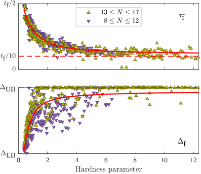
Figure 1: Optimum parameters of the linear schedules for the 500 representative graphs. These values depend on $\mathcal{HP}$ and converge quickly to a constant for sufficiently hard graphs. This behavior is particularly strong for $\tau_{\text{f}}$ (top) and $\Delta_{\text{f}}$ (bottom) at the end of the adiabatic evolution. There is no statistical difference between the smallest graphs (down purple triangles) and the largest ones (up yellow-green triangles).

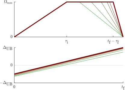
Figure 2: Optimized piecewise linear schedules with 4 free variables. The Rabi amplitude (top) and the detuning (bottom) depend on the hardness of the graph and are illustrated here for $\mathcal{HP}\in\{0.5,1,2,4,8\}$ (thin lines, from green to maroon) and in the limit $\mathcal{HP}\to\infty$ (dark maroon thick line). The optimized values become in this limit $\tau_{\text{i}}\approx t_{\text{f}}/2$, $\tau_{\text{f}}\approx t_{\text{f}}/10$, $\Delta_{\text{i}}\approx-\Delta_{\text{UB}}/2$, and $\Delta_{\text{f}}=\Delta_{\text{UB}}$.

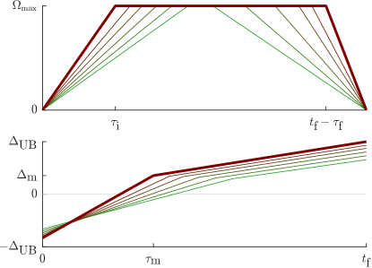
Figure 3: Optimized piecewise linear schedules with 6 free variables. In this case, $\tau_{\text{i}}$ dislays a clear dependence on $\mathcal{HP}$. In the limit of infinite hardness, the optimized values are $\tau_{\text{i}}\approx 0.22\,t_{\text{f}}$ and $\tau_{\text{f}}\approx 0.12\,t_{\text{f}}$ for the Rabi amplitude (top) and $\Delta_{\text{i}}\approx-0.83\,\Delta_{\text{UB}}$, $\tau_{\text{m}}\approx 0.34\,t_{\text{f}}$, $\Delta_{\text{m}}\approx 0.36\,\Delta_{\text{UB}}$, and $\Delta_{\text{f}}=\Delta_{\text{UB}}$ for the detuning (bottom).

The hardness-dependent linear schedules yield very good results compared to existing protocols, which motivates us to go one step further by considering two more degrees of freedom $(\tau_{\text{m}},\Delta_{\text{m}})$ for the detuning, see Fig. 3. The resulting optimized schedules are still easily implementable, yet they perform much better than all benchmark protocols, see Sec. 2.3.

A priori knowledge of the hardness parameter

The aim of the adiabatic evolution is to find the MIS of a graph, which in turn allows one to calculate the hardness of that very graph. In the case of small graphs, since all vertex configurations are enumerated effortlessly, we consider that $\mathcal{HP}$ is a known value that can be used to choose the best schedules from the fitted model. For large graphs, however, the hardness parameter cannot be considered to be known beforehand. In that case, one should either take the schedules in the limit $\mathcal{HP}\to\infty$, which yields quite good results for all graphs, or eventually apply a one-dimensional search on the hardness parameter, which is still much easier than performing a multi-dimensional optimization of all schedule parameters.

2.2 Counterdiabatic protocol

The limited coherence time of the quantum state in experiments is a major source of error in adiabatic computing. Well-established methods to overcome such limitations include the shortcuts to adiabadicity, among which is the counterdiabatic (CD) driving [36]. The idea of the CD driving is to add a gauge potential to the adiabatic Hamiltonian such that the transitions between eigenstates are suppressed during the evolution. However, the calculation of the exact gauge potential is a very difficult task in general, and these mathematical terms may not be always adapted to an experimental implementation. Nevertheless, by neglecting the interactions of the Rydberg Hamiltonian, one is able to find a suitable gauge potential which utilizes the phase of the Rabi drive [28]. In this study, we propose to generalize the adiabatic schedules of this so-called Analog Counterdiabatic Quantum Computing (ACQC) protocol as follows:

$$\Omega_{\text{ad}}(t) =\Omega_{\max}\,\sin\left(\frac{\pi}{2}\,\sin\left(\theta_{\Omega}(t)\right)\right)^{2},$$ (6a)

$$\Delta_{\text{ad}}(t) =\frac{\Delta_{\text{i}}+\Delta_{\text{f}}}{2}+\frac{\Delta_{\text{i}}-\Delta_{\text{f}}}{2}\cos\left(\theta_{\Delta}(t)\right),$$ (6b)

where $\theta(t)$ is any monotonic smooth function that ranges from $0$ to $\pi$; here we set $\theta_{\Omega,\Delta}(t)=\pi\,t/t_{\text{f}}$. Moreover, based on the variational procedure described in [27], we improve on the ACQC protocol by including the Rydberg interactions in the calculation of the CD terms, thus adapting the gauge potential to each different graph, see Appendix B. The detuning is not altered by this operation, whereas the Rabi drive becomes:

$$\Omega =\sqrt{\Omega_{\text{ad}}^{2}+\Omega_{\text{cd}}^{2}},$$ (7a)

$$\phi =\arctan(\Omega_{\text{cd}}/\Omega_{\text{ad}}),$$ (7b)

with

$$\Omega_{\text{cd}}=\frac{\Omega_{\text{ad}}\dot{\Delta}_{\text{ad}}-\dot{\Omega}_{\text{ad}}\Delta_{\text{ad}}+\dot{\Omega}_{\text{ad}}\,T_{1}\,\nu}{\Omega_{\text{ad}}^{2}+\Delta_{\text{ad}}^{2}-2\Delta_{\text{ad}}\,T_{1}\,\nu+T_{2}\,\nu^{2}}$$ (8)

and where $0\leq\nu\leq C_{6}/a^{6}$ is an additional free parameter that interpolates between the standard and the generalized gauge potentials. In the latter equation, the variables $T_{1}$ and $T_{2}$ depend on the interaction terms $V_{ij}$ and are therefore specific to the graph to be solved. As expected, the CD contribution vanishes for $t_{\text{f}}\to\infty$ since $\dot{\Omega}_{\text{ad}}$ and $\dot{\Delta}_{\text{ad}}$ tend to zero in this limit.

Similarly as for the piecewise linear protocol, we optimize the schedule parameters $(\Delta_{\text{i}},\Delta_{\text{f}},\nu)$ for all graphs of the dataset, see Fig. 4. The interpolating coefficient $\nu$ tends to a strictly positive value for the hardest graphs, indicating that the generalized gauge potential plays an important role in the CD protocol. Note that the easy graphs exhibit optimized values of $\Delta_{\text{f}}$ that are smaller than the statistically determined constant $\Delta_{\text{LB}}$. This is due to the fact that the exact lower bounds on the detuning are much smaller in that case, see Fig. 11 in the appendix. The shape of the CD phase is highly nontrivial, and we observe a strong shift toward higher values of the detuning for hard MIS instances, see Fig. 5. Finally, we also tried to further improve the results by considering more evolved $\theta$ functions—in particular, to mimic the skewed shape of the Rabi amplitude in Fig. 2—but no significant gain was found in this case.

Hardware implementation

In Aquila, the Rabi amplitude and the detuning must be defined as piecewise linear and not smooth functions, while the phase must be piecewise constant. However, the step size can be as small as 0.05 µs, which results in 80 intervals for the longest coherent evolution. The schedules are therefore well approximated in the quantum hardware, but one could slightly improve the experimental results by taking into account this hardware capability in the numerical simulations.

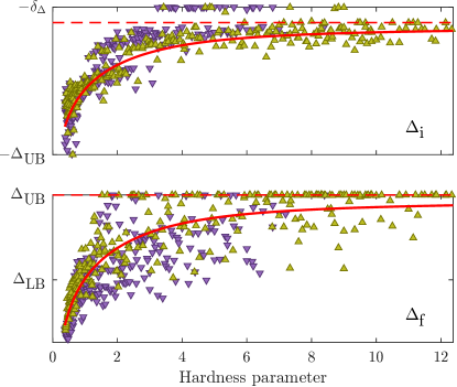
Figure 4: Optimum parameters for the CD schedules. The initial detuning (top) reaches the upper bound $-\delta_{\Delta}$ for several graphs but tends to a lower value $\Delta_{\text{i}}\approx-\Delta_{\text{UB}}/10$ for the hardest graphs. The final detuning (bottom) also increases with the hardness parameter and quickly reaches the limit $\Delta_{\text{UB}}$. The coefficient $\nu$ (not shown) displays a similar behavior and tends to $\nu=4.30$ in the current setting.

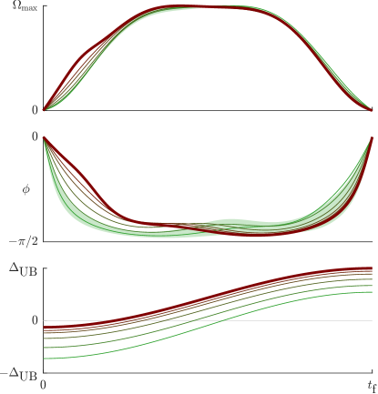
Figure 5: Optimized counterdiabatic schedules with 3 free variables. Unlike the detuning (bottom), the Rabi amplitude (top) and phase (middle) depend not only on $\mathcal{HP}$ but also on $t_{\text{f}}$ and on the graph-dependent variables $T_{1}$ and $T_{2}$. Here, the curves are displayed for $t_{\text{f}}=1$ and for the mean values of the dataset $\overline{T}_{1}\approx 0.93$ and $\overline{T}_{2}\approx 1.46$. The light green area represents the variation due solely to $T_{1}$ and $T_{2}$ for $\mathcal{HP}=0.5$.

2.3 Results

In Fig. 6, we compare the probability $P_{\text{MIS}}$ to reach the solution for 4 protocols: the piecewise linear and ACQC protocols defined in [28] which serve as benchmarks, and their generalized and hardness-dependent counterparts described in the previous sections. Note that $a=5.5$ for the benchmark protocols but $a=5$ in our study. The $\mathcal{HP}$-linear protocol (with 6 degrees of freedom) yields the best results for all graphs, and in particular for the hard ones with a tenfold improvement over the benchmark.

Graph-to-graph comparisons are illustrated in Fig. 7. As for the optimized schedule parameters, we observe that the values of $P_{\text{MIS}}$ depend mostly on the hardness parameter and not on the size of the graphs. For instance, the success probabilities for the $\mathcal{HP}$-linear protocol range from 0.59 ($\mathcal{HP}=4.20$) to 0.99 ($\mathcal{HP}=0.46$) for $N=10$, and from 0.11 ($\mathcal{HP}=9.71$) to 0.98 ($\mathcal{HP}=0.52$) for $N=17$.

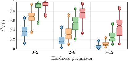
Figure 6: Box plot of the probability to reach the MIS depending on the hardness of the 500 graphs of the dataset. The piecewise linear (blue) and ACQC (orange) protocols serve as benchmarks. For hard graphs, the generalized $\mathcal{HP}$-ACQC (green) and $\mathcal{HP}$-linear (red) protocols developed in this study lead to an average success probability that is improved by approximately 150% and 1 000%, respectively.

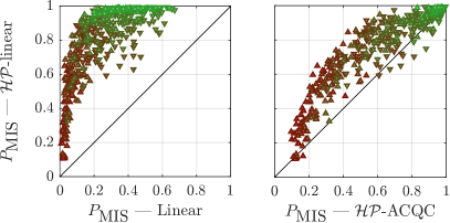
Figure 7: Graph-to-graph comparisons of $P_{\text{MIS}}$. Left: the $\mathcal{HP}$-linear protocol developed in this study leads to a 3.6-fold mean improvement on the linear protocol described in [28]. Right: except for rare instances, the hardness-dependent piecewise linear protocol always beats its ACQC counterpart. Note that $P_{\text{MIS}}$ depends strongly on $\mathcal{HP}$ but not on $N$ (upward or downward triangle), with low sucess probabilities for the hard graphs (maroon) and nearly perfect results for the easy ones (green).

3 Experiments

Based on thorough numerical simulations, we have shown in the previous section that hardness-dependent schedules lead to high probabilities to reach the MIS solution. Now, we extend these results to the hardware and to graphs that are not part of the dataset used in the optimization. First, we consider a small set of “toy graphs” that we can still simulate classically to ensure that the various protocols are correctly run in Aquila. Then, we apply the models to large graphs made up of 137 vertices to verify that the hardness parameter and not the size of the graph is indeed the most relevant property when solving the MIS problem.

Measurement shots

For all examples, we use 720 shots (repetitions of the adiabatic evolution) to get enough data for a statistical comparison of the methods. We choose this specific value because it is a multiple of 9, 12, and 16, which are the maximum number of copies of the small graphs ($3\times 3$ and $3\times 4$ lattices with $a=5$ and $a=5.5$) that fit and can be run simultaneously in the hardware. We consider only the shots in which the lattice is correctly filled by atoms. The typical probability of failing to occupy a site in Aquila is $\epsilon_{\text{fill}}=0.007$ [21, Sec. 1.5], and in practice we get $684\pm 7$ and $380\pm 14$ valid shots for the small and the large graphs, respectively.

3.1 Toy graphs

In Fig. 8, we display the probability to reach the MIS solution for the 11 toy graphs defined in [29]. As in that article, we set $t_{\text{f}}=0.7$ so that the probabilities of success are distributed around 50%. We observe a good agreement between numerical simulations and the corresponding results obtained on hardware, especially for the benchmark protocols. A possible reason for the optimized schedules to yield outcomes that are slightly lower than expected may be the choice of a smaller lattice spacing or the larger gradient of $\Omega$ at the end of the evolution; many other sources of error could explain these differences, see [21, Sec. 1.5] for an exhaustive list. Nevertheless, the $\mathcal{HP}$-linear protocol still performs better on the hardware than the linear and CD benchmarks, with a threefold and a twofold mean improvement, respectively.

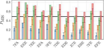
Figure 8: Probability to reach the MIS solution for the 11 toy graphs. The rectangle bars are numerical results and the error bars are experimental results (95% confidence intervals). The ranking of the 4 studied protocols is the same as in Fig. 6, with $\mathcal{HP}\in[2,3]$ here. The black horizontal line represents the average success probability obtained by the Bayesian optimization in [29, Fig. 9], which performs better than the benchmarks (blue and orange) but not as well as the hardness-dependent protocols (green and red).

3.2 Large graphs

We now turn to large graphs, which are of much higher interest in real applications. We consider three of the four graphs studied in [29, Fig. 10], which consist of 137 vertices and whose hardness parameters extend over three orders of magnitude ($\mathcal{HP}\approx$ 14, 126, and 1435). In addition, we generate one very easy graph of the same size to span yet another order of magnitude ($\mathcal{HP}\approx$ 1.4), see Fig. 9. The hardness parameter of these large graphs is efficiently computed by advanced classical algorithms, namely by the GenericTensorNetworks Julia library [37, 38].

Since the MIS solutions and consequently the hardness parameters are not known a priori, we apply our optimized linear schedules in the limit $\mathcal{HP}\to\infty$. Moreover, we set $t_{\text{f}}=t_{\text{max}}=4$ so that the probability to find a MIS solution is as high as possible. Finally, we post-process all experimental data such that the measured outcomes become valid maximal independent sets. To this end, we use the greedy procedure described in [19, Sec. S2.3]: first, we remove any of two neighboring vertices until the sets become independent. Second, we include a vertex at any free site with no neighbor until the sets are maximal. The same procedure applied to an empty configuration is used as a classical benchmark, which highlights the relative gain obtained with the quantum protocols [21, Sec. 6].

The results are summarized in Fig. 9: the MIS solution is never found by the classical greedy algorithm and is obtained by the standard linear protocol only for the easiest graph. On the contrary, the $\mathcal{HP}$-linear protocol leads to the solution for all but the hardest graph, which indicates a clear improvement over the existing protocols.

4 Discussion and outlook

In this work, we have shown how to design the adiabatic schedules of the Rydberg Hamiltonian to efficiently solve the MIS problem on unit disk graphs.

First, a statistical investigation of the conditions for which the final quantum state encodes the MIS solution has revealed that the final detuning should lie in a narrow interval. To our knowledge, these are the tightest bounds ever mentioned. We believe that choosing a final detuning in that interval would improve the results of many other studies, either in terms of success probability or number of optimization steps. In fact, applying adiabatic protocols in which the final ground state does not correspond to the sought solution can only lead to poorly performing algorithms.

Second, the individual optimization of numerous small graphs has shown that the optimum parameters of the schedules depend mostly on the hardness parameter and only marginally on the size of the graph. Through extensive classical simulations of small systems, we have generated adiabatic schedules that perform extremely well also when applied to much larger graphs; only the hardest instances are not solved by our protocol. Obviously, improvements in the hardware would greatly help in this regard, especially if it permits a longer coherent evolution time. Since the quantum technology evolves rapidly, this could be the case soon. However, because of the combinatorial nature of the hardness parameter, very hard MIS problems exist only in sufficiently large graphs, so that our numerical study should be extended to larger graphs to address this issue. We believe that improved schedules could be easily found by considering slightly larger systems, for instance up to about 25 vertices, or even larger ones using tensor network techniques for the simulations whenever appropriate [39].

We have focused our work on two families of schedules, namely piecewise linear and smooth counterdiabatic functions. The phase of the Rabi drive is nonconstant only in the latter case, and we have developed a generalized version of the ACQC protocol [28] to make it specific to each graph. However, when correctly parametrized, the somehow simpler $\mathcal{HP}$-linear protocol performs better in almost all numerical simulations. This difference is even more pronounced in experiments, as the smooth CD schedules have to be converted into piecewise linear or constant functions. We have used a maximum number of 6 free parameters in the optimization, but more general functions may be investigated since the method described in this work applies to any kind of schedules. Moreover, it would be interesting to develop models of optimized schedules that do not depend only on the hardness parameter but also on other global properties of the graphs, e.g., the mean degree or the mean eccentricity of the vertices. Based on machine learning, such additional predictors could in fact improve the fitting of the schedule parameters.

We think that hybrid classical-quantum algorithms could take advantage of our protocols and, more generally, of precomputed optimized schedules: instead of searching in the huge space of all parameters, one could consider lower-dimensional meaningful ansatzes, such as the $\mathcal{HP}$-parametrization of the schedules or the principal component of the residuals of the fitted parameters.

Finally, we believe that the piecewise linear protocols developed in this study should serve as a new benchmark for any future adiabatic algorithm that aims to solve the MIS problem with Rydberg atoms. In particular, the most basic version of this protocol with only 4 free parameters and in the limit of infinite hardness admits a very simple mathematical description, see Fig. 2, and it leads to relatively good results regardless of the specific graph to be solved.

The supporting data for this article are openly available on GitHub [40].

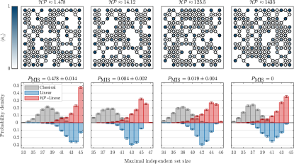
Figure 9: Experiments on large unit disk graphs. Top: four graphs with 137 vertices each and whose hardness parameters span four orders of magnitude; the three hardest graphs are taken from [29]. In shades of blue, the probability $\braket{\hat{n}_{i}}$ to measure the $i$-th atom in the Rydberg state $\ket{1}$ at the end of the $\mathcal{HP}$-linear protocol. Due to the high degeneracy of the MIS, some vertices are equally measured in the ground or excited state. Bottom: experimental results (after a minimal post-processing) to find an independent set of a given size, with the MIS solution at the rightmost bin. The error bars represent the 95% confidence intervals. The classical greedy algorithm (gray) fails to find the solution in all cases. The benchmark linear protocol (blue) reaches the MIS in the easiest case but fails for any harder instance. Finally, the $\mathcal{HP}$-linear protocol is able to find the MIS except for the hardest graph; the corresponding values of $P_{\text{MIS}}$ are indicated in the subtitles. The success probabilities for the two CD protocols (not shown) lie between those of the two linear protocols.

Appendix A Ground state encoding of the maximum independent set problem

Given a simple undirected graph $\mathcal{G}=(V,E)$ with vertex set $V$ and edges set $E$, a subset $S\subseteq V$ is called independent if no pair of vertices in $S$ are connected by an edge in $E$. In the maximum independent set (MIS) problem, we want to find the independent set of largest cardinality. Denoting by $x_{i}\in\{0,1\}$ the absence or the presence of the vertex $i=1,\ldots,N$ in $S$, it is proven that the MIS solution minimizes the cost function [41, 42]

$$\mathcal{C}(x_{1},\ldots,x_{N})=-\sum_{i\in V}\Delta\,x_{i}+\sum_{ij\in E}V_{ij}\,x_{i}x_{j}$$ (9)

if $0<\Delta<V_{ij}$ for all $ij\in E$. In analog quantum computing with arrays of Rydberg atoms, $\mathcal{G}$ is a unit disk graph that connects the nearest and next-nearest neighbors of a square lattice. Neglecting the interactions between farther atoms and for a non-planar graph (i.e., when crossing diagonals belong to it), the MIS condition becomes:

$$0<\Delta_{\text{f}}<\frac{C_{6}}{(\sqrt{2}\,a)^{6}}=\frac{V_{0}}{8},$$ (10)

where $a$ is the lattice spacing, $V_{0}=C_{6}/a^{6}$ is the interaction strength between adjacent atoms, and $\Delta_{\text{f}}=\Delta(t_{\text{f}})$ is the detuning at the final evolution time $t_{\text{f}}$. In several investigations, it is implicitly assumed that the inequalities (10) hold for all unit disk graphs due to the sharp Rydberg blockade transition. However, in what follows we show that the condition $0<\Delta_{\text{f}}$ is necessary but not sufficient.

A.1 Nonexistence of a lower bound on the detuning

The Van der Waals interaction decays quickly with the distance between atoms, but it cannot be neglected for distances close to the blockade radius. As an example, consider the graph that consists of three atoms in a row with a distance $2a$ between its extremities, see Fig. 10(a). In this case, the MIS solution is $(1,0,1)$, which corresponds to an energy $-2\Delta_{\text{f}}+V_{0}/64$. By listing the energy of all other configurations, we find the following conditions on $\Delta_{\text{f}}$ such that $\ket{101}$ is indeed the ground state of the final Rydberg Hamiltonian:

$$V_{0}/64<\Delta_{\text{f}}<2\,V_{0}.$$ (11)

The upper bound is of course already satisfied in Eq. (10) as it is a sufficient condition, but the value $V_{0}/64$ should be considered as a strict lower bound for any protocol; remark that this bound is mentioned in [21]. The question is then to determine if there exists, for unit disk graphs in a square lattice, a finite lower bound on the detuning to ensure the equivalence between the classical MIS solution and the ground state of the quantum Hamiltonian. Unfortunately, the answer is negative. In fact, consider the unit disk graph in Fig. 10(b), and the following two sets of vertices:

• the MIS solution with $m+1$ vertices on the main line (filled circles)

• the $m$ vertices located at the tip of the alternating upward and downward triangles (orange circles)

Taking into account all pairwise interactions, the corresponding energies read:

$$E_{0} =-(m+1)\,\Delta_{\text{f}}+\frac{V_{0}}{64}\sum_{i=1}^{m}\frac{m+1-i}{i^{6}},$$ (12a)

$$E_{1} =-m\,\Delta_{\text{f}}+\frac{V_{0}}{64}\sum_{i=1}^{\lfloor m/2\rfloor}\left(\frac{m+1-2i}{(4i^{2}-4i+2)^{3}}+\frac{m-2i}{(2i)^{6}}\right).$$ (12b)

For the ground state of the Hamiltonian to yield the MIS solution we must have $E_{0}<E_{1}$, i.e., the detuning has to satisfy the inequality

$$\frac{V_{0}}{64}\left(\Sigma_{0}-\Sigma_{1}\right)<\Delta_{\text{f}},$$ (13)

where $\Sigma_{0,1}$ stands for the sums in the r.h.s. of Eq. (12). However, one can check that the difference $\Sigma_{0}-\Sigma_{1}$ is always positive and becomes arbitrarily large for increasing $m$. In particular, this difference is larger than 8 for $m\geq 9$, leading to a contradiction with Eq. (10).

In conclusion, there does not exist a value of the final detuning such that the Rydberg Hamiltonian is ensured to encode the MIS solution of all unit disk graphs.

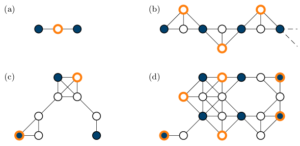
Figure 10: Examples of unit disk graphs to study the lower bound on the final detuning. The MIS solution (filled circles) has a lower energy than the suboptimal configuration (orange circles) iff $\Delta_{\text{f}}>\Delta_{\text{LB}}$. (a) Reference graph used in Eq. (11). (b) Graph with $N=3m+1$ vertices forming $m$ alternating upward and downward triangles. For any $\Delta_{\text{f}}>0$, there exists a value of $m$ such that the suboptimal configuration is energetically favorable. Finally, two non-planar graphs with very different lower bounds: (c) $\Delta_{\text{LB}}\approx V_{0}/1017$ ($\mathcal{HP}\approx 0.42$), and (d) $\Delta_{\text{LB}}\approx V_{0}/11.49$ ($\mathcal{HP}=15$).

A.2 Statistical analysis of the bounds on the detuning

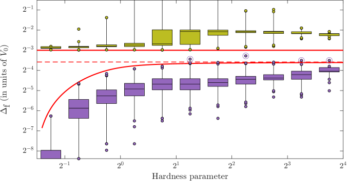
Figure 11: Box plot of the lower bounds $\Delta_{\text{LB}}$ (purple) and upper bounds $\Delta_{\text{UB}}$ (yellow-green) on the detuning $\Delta_{\text{f}}$ such that the ground state of the Hamiltonian encodes the MIS solution. Calculations have been performed on $10\,000$ non-isomorphic unit disk graphs with 8 to 19 vertices. All but 4 graphs satisfy $\Delta_{\text{LB}}\leq V_{0}/12$ (dashed red line) while $\Delta_{\text{UB}}$ is always strictly larger than $V_{0}/8$. It is interesting to note that, in average, easy graphs exhibit much smaller lower bounds than hard graphs (red curve), see also Fig. 10(c-d). Since the average value of $\Delta_{\text{LB}}$ quickly saturates for not-too-easy graphs, we are confident that these bounds can be effectively applied to graphs of any size.

As shown above, the final detuning has to be arbitrarily high if one wants to encode the MIS solution of any graph in the Rydberg Hamiltonian. However, this is not the case in general, as most graphs obey well-defined conditions on $\Delta_{\text{f}}$. Based on an extensive analysis of $10\,000$ graphs, see Fig. 11, we find that more than 99.9% of all graphs satisfy the following bounds:

$$\Delta_{\text{f}}\in[\Delta_{\text{LB}},\Delta_{\text{UB}}]=\left[\frac{V_{0}}{12}\,,\frac{V_{0}}{8}\right].$$ (14)

Interestingly, this interval is very close to the best range of parameters found by a variational optimization, see [21, Fig. 6.1], with $\Delta_{\text{LB}}=28.91$ and $\Delta_{\text{UB}}=43.36$ MHz for QuEra’s Aquila device and $a=5$ µm. Note that a statistical analysis is also performed in [19, Sec. S2], where it is stated that about 99% of the MIS problems can be encoded in the ground state of a Rydberg Hamiltonian for well-chosen fixed experimental parameters. We strongly recommend to consider the interval in Eq. (14) when setting the final detuning of any adiabatic protocol for the MIS problem. A value which lies far outside this interval will likely lead to poor numerical or experimental results simply because the ground state of the Hamiltonian does not correspond to the MIS solution.

Appendix B Graph-dependent counterdiabatic driving

For convenience, we set $\hbar=1$ and $\phi(t)=0$ in what follows, but all results can be extended to the general scenario. In this case, the Rydberg Hamiltonian reads:

$$H(t)=\frac{\Omega(t)}{2}\sum_{i}\hat{X}_{i}-\Delta(t)\sum_{i}\hat{n}_{i}+\sum_{i<j}V_{ij}\hat{n}_{i}\hat{n}_{j}\equiv\frac{\Omega(t)}{2}\ \hat{X}-\Delta(t)\ \hat{n}+\hat{V},$$ (15)

where $\hat{n}_{i}=\ket{1}_{i}\bra{1}$ and $\hat{X}_{i}$ is the Pauli matrix $\ket{0}_{i}\bra{1}+\ket{1}_{i}\bra{0}$ acting on the atom $i=1,\dotsc,N$.

B.1 Approximate adiabatic gauge potential

The idea of the CD driving is to add a gauge potential $\mathcal{A}$ to the Hamiltonian $H$ such that the transitions between eigenstates are suppressed during a shorten adiabatic evolution:

$$\widetilde{H}(t)=H(t)+\mathcal{A}(t),$$ (16)

where $\mathcal{A}$ satisfies the following equation [27, Eq. (2)]:

$$\left[\mathrm{i}\mkern 1.0mu\partial_{t}H-\left[\mathcal{A},H\right],H\right]=0.$$ (17)

Neglecting the interactions $\hat{V}$, it is shown in [28] that a solution of this equation exists:

$$\mathcal{A}_{V\rightarrow 0}=-\frac{1}{2}\ \frac{\Omega\dot{\Delta}-\dot{\Omega}\Delta}{\Omega^{2}+\Delta^{2}}\ \hat{Y}.$$ (18)

This gauge potential leads to improved results compared to a simple adiabatic protocol, but one might expect even better results with a gauge potential that explicitly depends on the coefficients $V_{ij}$, hence being specific to the graph to be solved. In order to find such a generalized gauge potential, we consider the variational procedure that consists in minimizing the action [27, Eq. (8)]

$$\mathcal{S}(\mathcal{A}_{\lambda})=\operatorname{Tr}\left(G^{2}(\mathcal{A}_{\lambda})\right)\quad\text{with}\quad G(\mathcal{A}_{\lambda})=\partial_{t}H+\mathrm{i}\mkern 1.0mu\ [\mathcal{A}_{\lambda},H].$$ (19)

Here, we use the ansatz $\mathcal{A}_{\lambda}=-\hat{Y}\lambda(t)/2$ since the one-body Pauli matrices $\hat{Y}_{i}$ are the only operators that contribute to the action while being experimentally implementable through the phase $\phi$ of the Rabi drive. One easily checks that $\mathcal{S}$ is quadratic in $\lambda$ and that the optimum value of this parameter is:

$$\lambda=2\,\frac{\operatorname{Tr}\left(\partial_{t}H\cdot[\mathrm{i}\mkern 1.0mu\hat{Y},H]\right)}{\operatorname{Tr}\left([\mathrm{i}\mkern 1.0mu\hat{Y},H]^{2}\right)}.$$ (20)

Based on the algebraic properties of the Pauli matrices and the trace operator, this expression can be developed and simplified as follows:

$$\lambda=\frac{\Omega\dot{\Delta}-\dot{\Omega}\Delta+\dot{\Omega}\ T_{1}}{\Omega^{2}+\Delta^{2}-2\Delta\ T_{1}+T_{2}},$$ (21)

where the normalized traces $T_{1}$ and $T_{2}$ are given by:

$$N\cdot T_{1} =2^{-N}\operatorname{Tr}\left(\hat{X}\cdot[\mathrm{i}\mkern 1.0mu\hat{Y},\hat{V}]\right)=\sum_{i<j}V_{ij},$$ (22a)

$$N\cdot T_{2} =2^{-N}\operatorname{Tr}\left([\mathrm{i}\mkern 1.0mu\hat{Y},\hat{V}]^{2}\right)=\frac{1}{2}\sum_{i\leq j}\sum_{k\neq i,j}V_{ik}V_{kj}.$$ (22b)

As expected, the graph-dependent gauge potential $\mathcal{A}_{\lambda}$ is equal to $\mathcal{A}_{V\rightarrow 0}$ in the case of vanishing interactions, with $T_{1}=T_{2}=0$ in this limit. Due to the fast-decaying interaction between distant atoms, $T_{1}$ and $T_{2}$ do not scale with $N$ as they represent average values of (nearly) local functions. For instance, $T_{1}$ is exactly half the mean degree of the underlying graph if ones considers its adjacency matrix instead of the interaction terms in Eq. (22a).

Finally, the driving amplitude and phase of the full Rydberg Hamiltonian $\widetilde{H}$ become:

$$\widetilde{\Omega}=\sqrt{\Omega^{2}+\lambda^{2}},$$ (23a)

$$\widetilde{\phi}=\arctan(\lambda/\Omega).$$ (23b)

Note that $\lambda$ and therefore $\dot{\Omega}$ should be equal to zero at the beginning and at the end of the protocol to satisfy the boundary conditions $\widetilde{\Omega}(t_{\text{i}})=\widetilde{\Omega}(t_{\text{f}})=0$.

B.2 Practical application of the counterdiabatic driving

Hardware implementation

It follows from Eq. (23a) that $\widetilde{\Omega}$ is always larger than $\Omega$, so that it may exceed the maximum Rabi frequency $\Omega_{\max}$ of the quantum computer. In this case, we rescale the adiabatic function $\Omega$ by a factor $0<\kappa<1$ to satisfy the hardware constraint at any time $t$ of the evolution:

$$\max_{t}\left\{\widetilde{\Omega}\big{(}\kappa\,\Omega(t),\Delta,T_{1},T_{2}\big{)}\right\}=\Omega_{\max}.$$

Note that this is slightly different from rescaling $\widetilde{\Omega}$ directly, as the relations (21, 23) would not hold in that case.

Variational parameter

Since Eq. (21) is a generalization of the counterdiabatic term proposed in [28] through the addition of $T_{1}$ and $T_{2}$, it is interesting in an optimization context to consider a continuous interpolation between these two protocols. One possibility is to consider the interaction strength $V_{0}$ as a free parameter in the range $[0,C_{6}/a^{6}]$ when calculating the CD driving. To avoid any confusion with the fixed interactions in the Rydberg Hamiltonian, we denote by $\nu$ this free parameter. Numerically, this is equivalent to replace $T_{1}$ and $T_{2}$ in Eq. (21) by the following expressions:

$$T_{1} =\nu\,T_{1}^{(0)},$$ (24a)

$$T_{2} =\nu^{2}\,T_{2}^{(0)},$$ (24b)

where $T_{1}^{(0)}$ and $T_{2}^{(0)}$ are the traces evaluated at $V_{0}=1$ in Eq. (22). Another possibility would be, e.g., to consider the two-variable parametrization $T_{i}=\nu_{i}\,T_{i}^{(0)}$, with $\nu_{i}\in[0,V_{0}^{i}]$ and $i\in\{1,2\}$.

Appendix C Graph datasets and numerical implementation

In the following sections, we first describe two sets of unit disk graphs $\mathcal{G}=(V,E)$ that are used in this study; the data are available on GitHub [40]. In all examples, we consider an underlying square lattice where the distance between nearest-neighbors is $a=1$ and where any pair of vertices in $V$ is connected by an edge in $E$ if the corresponding distance is smaller than or equal to $\sqrt{2}$. Then, we detail the numerical method that is used to simulate the evolution of the quantum state under the action of the Rydberg Hamiltonian.

C.1 Graph datasets

Small graphs

From $10\,000$ non-isomorphic graphs randomly generated, we choose 500 graphs such that the correlation between their hardness parameter and their order is as small as possible, see Fig. 12. More precisely, we apply the following rules to determine which graphs belong to the dataset:

• there are exactly 50 graphs for each order from 8 to 17

• the hardness parameters are distributed as evenly as possible in a log-scale from 0.375 to 12; in particular, no two graphs share the same hardness parameter, and exactly 100 graphs are contained in each bin $[3\cdot 2^{i-4},3\cdot 2^{i-3})$ with $i=1,\ldots,5$

• the distribution of the graph orders is as uniform as possible within each such bin

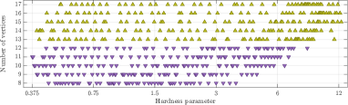
Figure 12: Visualization of the hardness parameters $\mathcal{HP}$ and the orders of the 500 small graphs. Due to the combinatorial definition of the hardness parameter, graphs with fewer vertices (down purple triangles) cannot generate very hard MIS instances. This explains why graphs of order 13 and more (up yellow-green triangles) are overrepresented in the range $\mathcal{HP}\in[6,12]$.

Toy graphs

For completeness, we display in Fig. 13 the 11 “toy graphs” defined in [29, Appendix C]:

• the underlying square lattice has $4\times 3$ sites

• the order of the graphs is 9 or 10

• there is only one MIS solution for each graph

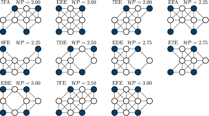
Figure 13: The 11 “toy graphs” sorted by the number of vertices (9 or 10) and by hardness parameter (between 2 and 3). The unique MIS is highlighted with dark blue circles. To refer to a specific graph, we generate the three-nibble identifiers as follows: the $i$-th nibble (four-bit aggregation) is the hexadecimal symbol that represents the absence or presence of a vertex in the 4 sites of the $i$-th row (from top to bottom).

C.2 Numerical implementation

Several software development kits (SDK) exist to simulate the Rydberg evolution: Bloqade [43] and Amazon Braket [32] for QuEra’s hardware, or Pulser [33] based on QuTiP for Pasqal’s technology, just to name a few. Nevertheless, we developed our own routines to get a full control over all parameters and, more importantly, to fit exactly our needs. In fact, optimizing hundreds of graphs for several protocols requires intense (classical) computing power, so that we have to find the perfect balance between accuracy and speed. For example, for each graph of the datasets we precompute all time- and protocol-independent terms in the Hamiltonian, namely the $\hat{X}$, $\hat{Y}$, $\hat{n}$ and $\hat{V}$ operators, see Eq. (15). We also use an explicit Runge-Kutta method of order 2 [44] to integrate the time-dependent Schrödinger equation, which turns out to be sufficiently accurate and much faster than the default order 8 method (DOP853 in Python or Vern8 in Julia). The initial state of this ordinary differential equation is $\ket{0}^{\otimes N}$, which corresponds to the unique ground state of the Rydberg Hamiltonian with $\Omega=0$ and $\Delta<0$.

Blockade subspace

Besides the above-mentioned implementation aspects, a crucial ingredient is the correct use of the blockade subspace: when the interaction energy between Rydberg states is much larger than the Rabi strength, the exact dynamics in the full Hilbert space is well approximated by the dynamics in the subspace where only one Rydberg excitation is allowed between nearby atoms [45]. In numerical simulations, the states $\ket{11}_{ij}$ are therefore neglected if the distance between $i$ and $j$ is smaller than a given subspace radius $R_{\text{s}}$, which results in much faster computations. The default setting in most programs is $R_{\text{s}}=R_{\text{b}}$, so that the quantum evolution is restricted to the independent sets in unit disk graphs. However, this approximation is too coarse to get accurate results, see Fig. 14: neglecting the states $\ket{11}$ for next-nearest neighbors (extremities of a diagonal) leads to success probabilities that are overestimated by up to 50%. Therefore, it is crucial to simulate either the full Hilbert space or the blockade subspace where only nearest neighbor Rydberg states are neglected.

Optimization algorithm

In this study, we focus on the probability to reach a MIS, i.e., we want to maximize the overlap between the quantum state at the end of the evolution and all MIS solutions of the graph under investigation, see Eq. (5). The set of parameters $\Theta$ to be optimized depends on the protocol, e.g., $\Theta=(\tau_{\text{i}},\tau_{\text{f}},\Delta_{\text{i}},\Delta_{\text{f}})$ for the simple linear schedules. Since the Schrödinger evolution is deterministic and that we simulate noiseless systems, any standard optimization algorithm may be applied. We choose the simplex search method [46], which turns out to be robust and very efficient in our setting. Finally, we set $t_{\text{f}}=1$ µs, which leads to success probabilities that are well distributed over the whole unit interval for the 500 graphs of the dataset.

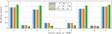
Figure 14: Numerical simulations of the Rydberg Hamiltonian for the toy graph “7DE” and the ACQC protocol defined in [28] with $t_{\text{f}}=1$ µs. The height of the bars represents the probability to find the atom $i$ in the state $\ket{1}$ at the end of the evolution, with $i=1,\ldots,9$ from top to bottom and left to right in the graph. The MIS solution (1, 3, 7, 9) is clearly visible in this bar chart. We verify that our implementation (light colors) is perfectly equivalent to that of Bloqade (dark colors); note that, depending on the SDK, the phase has to be multiplied by minus one in Eq. (23b). We also observe that the simulations in the full Hilbert space (blue bars) match those performed in the blockade subspace of nearest neighbors (orange bars). However, the unit disk subspace approximation $R_{\text{s}}=R_{\text{b}}$ (green bars) is clearly in favor of the MIS solution and thus cannot be considered as satisfactory. This is even more noticeable when comparing the probability to reach the ground state at the end of the evolution for each blockade subspace: 0.49(4), 0.49(6), and 0.70(0) respectively.

References

- [1] Francesco Bova, Avi Goldfarb, and Roger G. Melko. “Commercial applications of quantum computing”. EPJ Quantum Technology 8, 2 (2021).
- [2] Amira Abbas, Andris Ambainis, Brandon Augustino, Andreas Bärtschi, Harry Buhrman, Carleton Coffrin, Giorgio Cortiana, Vedran Dunjko, Daniel J. Egger, Bruce G. Elmegreen, Nicola Franco, Filippo Fratini, Bryce Fuller, Julien Gacon, Constantin Gonciulea, Sander Gribling, Swati Gupta, Stuart Hadfield, Raoul Heese, Gerhard Kircher, Thomas Kleinert, Thorsten Koch, Georgios Korpas, Steve Lenk, Jakub Marecek, Vanio Markov, Guglielmo Mazzola, Stefano Mensa, Naeimeh Mohseni, Giacomo Nannicini, Corey O’Meara, Elena Peña Tapia, Sebastian Pokutta, Manuel Proissl, Patrick Rebentrost, Emre Sahin, Benjamin C. B. Symons, Sabine Tornow, Victor Valls, Stefan Woerner, Mira L. Wolf-Bauwens, Jon Yard, Sheir Yarkoni, Dirk Zechiel, Sergiy Zhuk, and Christa Zoufal. “Quantum optimization: Potential, challenges, and the path forward” (2023). arXiv:2312.02279.
- [3] Rhonda Au-Yeung, Nicholas Chancellor, and Pascal Halffmann. “NP-hard but no longer hard to solve? Using quantum computing to tackle optimization problems”. Frontiers in Quantum Science and Technology2 (2023).
- [4] Karen Wintersperger, Florian Dommert, Thomas Ehmer, Andrey Hoursanov, Johannes Klepsch, Wolfgang Mauerer, Georg Reuber, Thomas Strohm, Ming Yin, and Sebastian Luber. “Neutral atom quantum computing hardware: performance and end-user perspective”. EPJ Quantum Technology 10, 32 (2023).
- [5] Edward Farhi, Jeffrey Goldstone, Sam Gutmann, Joshua Lapan, Andrew Lundgren, and Daniel Preda. “A quantum adiabatic evolution algorithm applied to random instances of an NP-complete problem”. Science 292, 472–475 (2001).
- [6] Andrew Lucas. “Ising formulations of many NP problems”. Frontiers in Physics2 (2014).
- [7] Tameem Albash and Daniel A. Lidar. “Adiabatic quantum computation”. Rev. Mod. Phys. 90, 015002 (2018).
- [8] Erica K. Grant and Travis S. Humble. “Adiabatic quantum computing and quantum annealing”. Oxford University Press (2020).
- [9] Adolfo del Campo. “Shortcuts to adiabaticity by counterdiabatic driving”. Phys. Rev. Lett. 111, 100502 (2013).
- [10] Masaki Ohkuwa, Hidetoshi Nishimori, and Daniel A. Lidar. “Reverse annealing for the fully connected -spin model”. Phys. Rev. A 98, 022314 (2018).
- [11] E. J. Crosson and D. A. Lidar. “Prospects for quantum enhancement with diabatic quantum annealing”. Nature Reviews Physics 3, 466–489 (2021).
- [12] Benjamin F. Schiffer, Jordi Tura, and J. Ignacio Cirac. “Adiabatic spectroscopy and a variational quantum adiabatic algorithm”. PRX Quantum 3, 020347 (2022).
- [13] Jonathan Wurtz, Pedro L. S. Lopes, Christoph Gorgulla, Nathan Gemelke, Alexander Keesling, and Shengtao Wang. “Industry applications of neutral-atom quantum computing solving independent set problems” (2024). arXiv:2205.08500.
- [14] Richard M. Karp. “Reducibility among combinatorial problems”. Pages 85–103. Springer US. Boston, MA (1972).
- [15] Brent N. Clark, Charles J. Colbourn, and David S. Johnson. “Unit disk graphs”. Discrete Mathematics 86, 165–177 (1990).
- [16] Ruben S. Andrist, Martin J. A. Schuetz, Pierre Minssen, Romina Yalovetzky, Shouvanik Chakrabarti, Dylan Herman, Niraj Kumar, Grant Salton, Ruslan Shaydulin, Yue Sun, Marco Pistoia, and Helmut G. Katzgraber. “Hardness of the maximum-independent-set problem on unit-disk graphs and prospects for quantum speedups”. Phys. Rev. Res. 5, 043277 (2023).
- [17] Hannes Pichler, Sheng-Tao Wang, Leo Zhou, Soonwon Choi, and Mikhail D. Lukin. “Quantum optimization for maximum independent set using rydberg atom arrays” (2018). arXiv:1808.10816.
- [18] Loïc Henriet, Lucas Beguin, Adrien Signoles, Thierry Lahaye, Antoine Browaeys, Georges-Olivier Reymond, and Christophe Jurczak. “Quantum computing with neutral atoms”. Quantum 4, 327 (2020).
- [19] S. Ebadi, A. Keesling, M. Cain, T. T. Wang, H. Levine, D. Bluvstein, G. Semeghini, A. Omran, J.-G. Liu, R. Samajdar, X.-Z. Luo, B. Nash, X. Gao, B. Barak, E. Farhi, S. Sachdev, N. Gemelke, L. Zhou, S. Choi, H. Pichler, S.-T. Wang, M. Greiner, V. Vuletić, and M. D. Lukin. “Quantum optimization of maximum independent set using rydberg atom arrays”. Science 376, 1209–1215 (2022).
- [20] M. D. Lukin, M. Fleischhauer, R. Cote, L. M. Duan, D. Jaksch, J. I. Cirac, and P. Zoller. “Dipole blockade and quantum information processing in mesoscopic atomic ensembles”. Phys. Rev. Lett. 87, 037901 (2001).
- [21] Jonathan Wurtz, Alexei Bylinskii, Boris Braverman, Jesse Amato-Grill, Sergio H. Cantu, Florian Huber, Alexander Lukin, Fangli Liu, Phillip Weinberg, John Long, Sheng-Tao Wang, Nathan Gemelke, and Alexander Keesling. “Aquila: Quera’s 256-qubit neutral-atom quantum computer” (2023). arXiv:2306.11727.
- [22] Edward Farhi, Jeffrey Goldstone, and Sam Gutmann. “A quantum approximate optimization algorithm” (2014). arXiv:1411.4028.
- [23] Nikolaj Moll, Panagiotis Barkoutsos, Lev S Bishop, Jerry M Chow, Andrew Cross, Daniel J Egger, Stefan Filipp, Andreas Fuhrer, Jay M Gambetta, Marc Ganzhorn, Abhinav Kandala, Antonio Mezzacapo, Peter Müller, Walter Riess, Gian Salis, John Smolin, Ivano Tavernelli, and Kristan Temme. “Quantum optimization using variational algorithms on near-term quantum devices”. Quantum Science and Technology 3, 030503 (2018).
- [24] M. Cerezo, Andrew Arrasmith, Ryan Babbush, Simon C. Benjamin, Suguru Endo, Keisuke Fujii, Jarrod R. McClean, Kosuke Mitarai, Xiao Yuan, Lukasz Cincio, and Patrick J. Coles. “Variational quantum algorithms”. Nature Reviews Physics 3, 625–644 (2021).
- [25] Mustafa Demirplak and Stuart A. Rice. “Adiabatic population transfer with control fields”. The Journal of Physical Chemistry A 107, 9937–9945 (2003). arXiv:https://doi.org/10.1021/jp030708a.
- [26] M V Berry. “Transitionless quantum driving”. Journal of Physics A: Mathematical and Theoretical 42, 365303 (2009).
- [27] Dries Sels and Anatoli Polkovnikov. “Minimizing irreversible losses in quantum systems by local counterdiabatic driving”. Proceedings of the National Academy of Sciences 114, E3909–E3916 (2017).
- [28] Qi Zhang, Narendra N. Hegade, Alejandro Gomez Cadavid, Lucas Lassablière, Jan Trautmann, Sébastien Perseguers, Enrique Solano, Loïc Henriet, and Eric Michon. “Analog counterdiabatic quantum computing” (2024). arXiv:2405.14829.
- [29] Jernej Rudi Finžgar, Martin J. A. Schuetz, J. Kyle Brubaker, Hidetoshi Nishimori, and Helmut G. Katzgraber. “Designing quantum annealing schedules using bayesian optimization”. Phys. Rev. Res. 6, 023063 (2024).
- [30] Wesley da Silva Coelho, Mauro D’Arcangelo, and Louis-Paul Henry. “Efficient protocol for solving combinatorial graph problems on neutral-atom quantum processors” (2022). arXiv:2207.13030.
- [31] Xiaozhen Ge, Re-Bing Wu, and Herschel Rabitz. “The optimization landscape of hybrid quantum–classical algorithms: From quantum control to nisq applications”. Annual Reviews in Control 54, 314–323 (2022).
- [32] Amazon Web Services. “Quantum computing with neutral atoms”. https://aws.amazon.com/braket/quantum-computers/quera/. Accessed: 2024-09-25.
- [33] Henrique Silvério, Sebastián Grijalva, Constantin Dalyac, Lucas Leclerc, Peter J. Karalekas, Nathan Shammah, Mourad Beji, Louis-Paul Henry, and Loïc Henriet. “Pulser: An open-source package for the design of pulse sequences in programmable neutral-atom arrays”. Quantum 6, 629 (2022).
- [34] Lucas Leclerc. “Quantum computing with Rydberg atoms: control and modelling for quantum simulation and practical algorithms”. Theses. Université Paris-Saclay. (2024). url: https://pastel.hal.science/tel-04745992.
- [35] Kangheun Kim, Minhyuk Kim, Juyoung Park, Andrew Byun, and Jaewook Ahn. “Quantum computing dataset of maximum independent set problem on king lattice of over hundred rydberg atoms”. Scientific Data 11, 111 (2024).
- [36] D. Guéry-Odelin, A. Ruschhaupt, A. Kiely, E. Torrontegui, S. Martínez-Garaot, and J. G. Muga. “Shortcuts to adiabaticity: Concepts, methods, and applications”. Rev. Mod. Phys. 91, 045001 (2019).
- [37] Jin-Guo Liu, Lei Wang, and Pan Zhang. “Tropical tensor network for ground states of spin glasses”. Physical Review Letters126 (2021).
- [38] Jin-Guo Liu, Xun Gao, Madelyn Cain, Mikhail D. Lukin, and Sheng-Tao Wang. “Computing solution space properties of combinatorial optimization problems via generic tensor networks”. SIAM Journal on Scientific Computing 45, A1239–A1270 (2023).
- [39] Román Orús. “Tensor networks for complex quantum systems”. Nature Reviews Physics 1, 538–550 (2019).
- [40] Sébastien Perseguers. “GitHub repository of Gradiom Sàrl”. https://github.com/Gradiom/quantum/ (2024).
- [41] Endre Boros and Peter L. Hammer. “Pseudo-boolean optimization”. Discrete Applied Mathematics 123, 155–225 (2002).
- [42] Vicky Choi. “Minor-embedding in adiabatic quantum computation: I. the parameter setting problem”. Quantum Information Processing 7, 193–209 (2008).
- [43] Phillip Weinberg, Kai-Hsin Wu, John Long, and Xiu-zhe (Roger) Luo. “QuEraComputing/bloqade-python: v0.15.11”. Zenodo (2024).
- [44] P. Bogacki and L.F. Shampine. “A 3(2) pair of Runge–Kutta formulas”. Applied Mathematics Letters 2, 321–325 (1989).
- [45] QuEra Computing. “Tutorials: Rydberg blockade”. https://queracomputing.github.io/Bloqade.jl/stable/tutorials/1.blockade/main/. Accessed: 2024-09-30.
- [46] Jeffrey C. Lagarias, James A. Reeds, Margaret H. Wright, and Paul E. Wright. “Convergence properties of the Nelder-Mead simplex method in low dimensions”. SIAM J. Optim. 9, 112–147 (1998).