Block coupling and rapidly mixing $k$-heights

Abstract

A $k$-height on a graph $G=(V,E)$ is an assignment $V\to\{0,\ldots,k\}$ such that the value on ajacent vertices differs by at most $1$. We study the Markov chain on $k$-heights that in each step selects a vertex at random, and, if admissible, increases or decreases the value at this vertex by one. In the cases of $2$-heights and $3$-heights we show that this Markov chain is rapidly mixing on certain families of grid-like graphs and on planar cubic $3$-connected graphs.

The result is based on a novel technique called block coupling, which is derived from the well-established monotone coupling approach. This technique may also be effective when analyzing other Markov chains that operate on configurations of spin systems that form a distributive lattice. It is therefore of independent interest.

1 Introduction

Markov chains are a generic approach to randomly sample an element from a collection of combinatorial objects. Examples where Markov chains have been proven useful include linear extensions [19, 11, 6, 29, 16], eulerian orientations [23], graph colorings [12] and chambers in hyperplane arrangements [4]. See [18] or [20] for more examples. One is usually interested in rapidly mixing Markov chains, i.e., Markov chains which converge fast towards their stationary distribution. Here we study a natural Markov chain $\mathcal{M}$ that operates on the set of so called $k$-heights of some fixed graph $G$. We identify a condition on a family $\mathcal{G}$ of graphs which implies that $\mathcal{M}$ is rapidly mixing on graphs in $\mathcal{G}$.

For a fixed graph $G=(V,E)$ and a fixed integral upper bound $k\in\mathbb{N}$, a $k$-height is an assignment $\varphi:V\to\{0,\ldots,k\}$ such that $\lvert\varphi(v)-\varphi(w)\rvert\leq 1$ for every edge $\{v,w\}\in E$. See Figure 1 for an example. In the case in which $G$ is a grid-like planar graph one may consider a $k$-height as height values of grid points or as a landscape satisfying a certain smoothness condition. The set of $k$-heights can also be described as feasible configurations of a certain spin system with uniform weights; in Section 5 we discuss this connection.

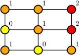
Figure 1: Example of a $2$-height. Colors visualize the values as a heat map.

1.1 Obtaining $k$-heights from $\alpha$-orientations

A motivation for studying $k$-heights stems from their connection to $\alpha$-orientations as studied in [10]. Given an embedded plane graph $G=(V,E)$ and a mapping $\alpha:V\to\mathbb{N}$, an $\alpha$-orientation of $G$ is an orientation of $E$ in which each vertex $v\in V$ has out-degree $\operatorname{outdeg}(v)=\alpha(v)$. In the example shown in Figure 2 we have $\alpha(v):=2$ for all $v\in V$.

The set of all $\alpha$-orientations of a planar graph $G$ forms a distributive lattice. There is a unique minimum $\alpha$-orientation $\overrightarrow{E}_{\text{min}}$ in which there is no bounded face whose bounding edges form a counterclockwise oriented cycle. The minimum $\overrightarrow{E}_{\text{min}}$ can be reached from every $\alpha$-orientation by a sequence of flips. A flip reverts the counterclockwise oriented bounding edges of a face into clockwise orientation, see the example in Figure 2.

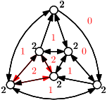
(a)

(b)

(c)

Figure 2: (a) Example of an $\alpha$-orientation $\overrightarrow{E}_{0}$. (b) the $\alpha$-orientation obtained by flipping the face bounded by the red arcs. (c) Minimal $\alpha$-orientation $\overrightarrow{E}_{\text{min}}$. Red numbers record the number of face flips needed to reach $\overrightarrow{E}_{0}$.

The numbers of flips on each bounded face that are necessary to reach $\overrightarrow{E}_{\text{min}}$ from $\overrightarrow{E}_{0}$ are independent of the choice of the flip sequence and uniquely determine $\overrightarrow{E}_{0}$. For a sufficiently large $k\in\mathbb{N}$, they form a $k$-height of the dual graph of $G$, in which the vertex corresponding to the unbounded face has value $0$; see Figure 2(c).

1.2 Rapidly mixing Markov chains on $k$-heights

The state space of the up/down Markov chain $\mathcal{M}$ is the set of $k$-heights of $G$. A transition of $\mathcal{M}$ depends on a vertex $\tilde{v}\in V$ and a direction $\triangle\in\{-1,+1\}$; both are chosen uniformly at random. According to $\triangle$, the value at $\tilde{v}$ is decremented or incremented. If the result is again a valid $k$-height, it is accepted as next state; otherwise, $\mathcal{M}$ stays at the same state. It is easy to see that the up/down Markov chain $\mathcal{M}$ is aperiodic, irreducible and symmetric, hence it converges towards the uniform distribution on the set of $k$-heights of $G$.

We could not prove that $\mathcal{M}$ is rapidly mixing via a direct application of one of the standard methods such as coupling or canonical paths (cf. [13]). Therefore, we introduce an auxiliary Markov chain $\mathcal{M}_{\mathcal{B}}$. It depends on some family $\mathcal{B}\subset\mathcal{P}(V)$ of blocks. A block is a set of vertices; together they cover $V$, i.e., each vertex $v\in V$ is contained in at least one block $B\in\mathcal{B}$. The chain $\mathcal{M}_{\mathcal{B}}$ also operates on the set of $k$-heights, but in each transition it does not just alter the value at a single vertex. Instead, it resamples the assgined values on an entire block at once.

A transition of $\mathcal{M}_{\mathcal{B}}$ can be simulated by a sequence of transitions of $\mathcal{M}$. Therefore, the comparison theorem of Randall and Tetali (2000) can be used to transform an upper bound on the mixing time of $\mathcal{M}_{\mathcal{B}}$ to an upper bound on the mixing time of $\mathcal{M}$. The idea to study a Markov chain $\mathcal{M}$ by first studying a boosted chain $\mathcal{M}_{\mathcal{B}}$ that performs block moves rather than single moves is also known in the context of Glauber dynamics under the term block dynamics; see [7, 22, 28].

Our main result is an upper bound on the mixing time of $\mathcal{M}$ that depends on a careful choice of $\mathcal{B}$. In the statement of the theorem we let $\partial B$ denote the boundary of a block $B\in\mathcal{B}$, i.e., the set of vertices outside of $B$ that are adjacent to $B$. The block divergence $E_{B,v}$ measures the influence of an increment on $v\in\partial B$ when resampling $B$. We will provide a precise definition of $E_{B,v}$ in Subsection 2.4.

Theorem 1.

Let $G=(V,E)$ be a finite graph, and $\mathcal{B}$ be a finite family of blocks, such that for every vertex $v\in V$ there is at least one $B\in\mathcal{B}$ with $v\in B$. If there exists $\beta<1$ such that for all $v\in V$

$$1-\frac{1}{2\lvert\mathcal{B}\rvert}\left(\#\{B\in\mathcal{B}\;\mid\;v\in B\}\hskip 5.69046pt-\sum_{B\in\mathcal{B}\;\mid\;v\in\partial B}(E_{B,v}-1)\right)\leq\beta<1\hskip 2.84544pt,$$

then for the mixing time $\tau(\varepsilon)$ of the up/down Markov chain $\mathcal{M}$ on $k$-heights of $G$ we have

$$\tau(\varepsilon)\leq c_{\mathcal{B},k}\cdot\frac{\left(\left(\log(\frac{1}{\varepsilon})\cdot\lvert V\rvert\right)+{\lvert V\rvert}^{2}\cdot\log(k+1)\right)\cdot\log\left(\frac{k\lvert V\rvert}{\varepsilon}\right)}{\log(\frac{1}{2\varepsilon})}\hskip 2.84544pt,$$

where

$$c_{\mathcal{B},k}:=\frac{8\cdot bmk(k+1)^{b}}{(1-\beta)\lvert\mathcal{B}\rvert}\hskip 2.84544pt$$

with $m:=\max_{v\in V}\#\{B\in\mathcal{B}\;\mid\;v\in B\}$ and $b:=\max_{B\in\mathcal{B}}\;\lvert B\rvert$.

A simplified but weaker version of Theorem 1 is given by its following corollary:

Corollary 1.

Let $G=(V,E)$ be a finite graph, and $\mathcal{B}$ be a finite family of blocks such that each vertex $v\in V$ is contained in at least $\check{m}$ blocks and in at most $s$ boundaries of blocks, and let $E_{\textup{max}}:=\max_{B\in\mathcal{B},v\in\partial B}E_{B,v}$. If there is a $\beta<1$ such that

$$1-\frac{1}{2\lvert\mathcal{B}\rvert}\left(\check{m}-s\cdot(E_{\textup{max}}-1)\right)\leq\beta\hskip 2.84544pt,$$

then the upper bound on $\tau(\varepsilon)$ given in Theorem 1 holds.

Below, we present various applications of Theorem 1 by showing that the assumptions are satisfied for different families of graphs and carefully selected families of blocks $\mathcal{B}$. Due to limited computational power, so far we were able to find appropriate upper bounds on $E_{\text{max}}$ only in the cases $k\in\{2,3\}$. Note that the up/down Markov chain $\mathcal{M}$ is trivially rapidly mixing when $k\in\{0,1\}$.

A bound for the mixing time of the up/down Markov-chain $\mathcal{M}$ operating on $k$-heights of $G$ which is of the form

$$\tau(\varepsilon)<c_{k}\cdot\frac{\left(\left(\log(\frac{1}{\varepsilon})\cdot n\right)+n^{2}\cdot\log(k+1)\right)\cdot\log\left(\frac{kn}{\varepsilon}\right)}{\log(\frac{1}{2\varepsilon})}\in\mathcal{O}\left(n^{2}\log n\right),$$

can be shown for the following pairs of an $n$ vertex graph $G$ and a $k$:

• Graph $G$ is a toroidal hexagonal grid graph and $k\in\{2,3\}$ with corresponding constants $c_{2}=1.747648\cdot 10^{5}$ and $c_{3}=1.052669\cdot 10^{7}$. (This is Theorem 7 in Subsection 4.2.)

• Graph $G$ is a toroidal rectangular grid graph and $k\in\{2,3\}$ with corresponding constants $c_{2}=2.844202\cdot 10^{10}$ and $c_{3}=1.333706\cdot 10^{13}$. (This is Theorem 6 in Subsection 4.1.)

• Graph $G$ is a simple $2$-connected $3$-regular planar graph and $k=2$ with corresponding constants $c_{2}=4.391132\cdot 10^{7}$. (This is Theorem 8 part (1) in Subsection 4.3.)

• Graph $G$ is a simple $3$-connected $3$-regular planar graph and $k\in\{2,3\}$ with corresponding constants $c_{2}=2.195097\cdot 10^{7}$ and $c_{3}=4.852027\cdot 10^{9}$.

  If $G$ is the dual graph of a $4$-connected triangulation, the constant for the case $k=2$ can be improved to $c_{2}=1.489256\cdot 10^{7}$.

  (This is Theorem 8 parts (2) and (3) in Subsection 4.3.)

We conjecture that the up/down Markov-chain is rapidly mixing on the $k$-heights of these graph classes for all $k$.

Our method can be applied to further families of graphs. The crucial step is to find an appropriate family of blocks $\mathcal{B}$ and a sharp analysis of $E_{B,v}$. Moreover, we believe that block coupling can be applied for proving that several other related Markov chains which also operate on a distributive lattice structure are rapidly mixing. An example could be generalized $k$-heights which allow a larger difference between the assigned values of two adjacent vertices.

Preliminary work of this research can be found in a PhD thesis [15].

1.3 Outline

In Section 2 we fix standard terminology related to Markov chains, give formal definitions for both Markov chains $\mathcal{M}$ and $\mathcal{M}_{\mathcal{B}}$ and introduce the proof ingredients for Theorem 1. The proof of Theorem 1 itself is presented in Section 3 and consists mainly of defining and analysing a monotone coupling of the Markov chain $\mathcal{M}_{\mathcal{B}}$. In Section 4 we show how to apply Theorem 1 and Corollary 1 in order to prove Theorem 7, Theorem 6 and Theorem 8. Finally, in Section 5 we relate $k$-heights to spin systems and discuss the applicability of a recent result by Blanca et al. [3] on bounding the mixing time of corresponding Glauber dynamics.

2 Preliminaries

2.1 Markov chains, mixing time and couplings

For a thorough introduction to the theory of discrete-time Markov chains we refer the reader to the recent book by Levin, Peres & Wilmer [20] or to the book by Jerrum [17, ch. 3-5]. Throughout this article, all Markov chains $\mathcal{C}=(X_{t})_{t\in\mathbb{N}}$ are discrete-time Markov chains on some finite state space $\mathcal{X}$. Moreover, they fulfill the following properties:

• Homogeneous: The transition probabilities

  $$\mathcal{C}(x,y):=\operatorname{Prob}[X_{t+1}=y\;\mid\;X_{t}=x]$$

  are constant over time, i.e. independent of $t$.

• Irreducible: Each state can be reached from any other state in a sequence of transitions with non-zero probability.

• Aperiodic: The possible number of steps for returning from a state to the same state again are not only multiples of some period $m\in\mathbb{N},m\geq 2$.

• Symmetric: We have $\mathcal{C}(x,y)=\mathcal{C}(y,x)$ for all $x,y\in\mathcal{X}$.

It is well-known that under these conditions the distribution of $X_{t}$ converges towards the uniform distribution on $\mathcal{X}$, which we denote by $\mathcal{U}(\mathcal{X})$. We want to analyse whether this convergence happens in polynomial time. To make this precise, let

$$\mathcal{C}^{t}(x,y):=\operatorname{Prob}[X_{t}=y\;\mid\;X_{0}=x]$$

and let $\mathcal{C}^{t}(x,\cdot)$ be the distribution of $X_{t}$ when $\mathcal{C}$ starts in state $X_{0}=x$. For any two probability measures $\mu,\mu^{\prime}$ on $\mathcal{X}$ the total variation distance is defined as

$$\lVert\mu-\mu^{\prime}\rVert_{TV}:=\max_{A\subset\mathcal{X}}\;\lvert\mu(A)-\mu^{\prime}(A)\rvert\hskip 2.84544pt.$$

Now,

$$d(t):=\max_{x\in\mathcal{X}}\;\lVert\mathcal{C}^{t}(x,\cdot)-\mathcal{U}(\mathcal{X})\rVert_{TV}$$

measures the worst-case distance of $\mathcal{C}$ to the uniform distribution after $t$ steps. Hence, the mixing time defined as

$$\tau(\varepsilon):=\min\{t\in\mathbb{N}\;\mid\;d(t)<\varepsilon\}\hskip 2.84544pt,$$

measures the number of time steps required for $\mathcal{C}$ to be $\varepsilon$-close to the uniform distribution. We say that $\mathcal{C}$ is rapidly mixing, if $\tau_{\mathcal{C}}(\varepsilon)$ is upper bounded by a polynomial in $\log(\lvert\mathcal{X}\rvert)$ and $\log(\varepsilon^{-1})$.

A common technique to prove that a Markov chain is rapidly mixing is by using a coupling. A coupling of a Markov chain $\mathcal{C}$ is another Markov chain $(X_{t},Y_{t})$ operating on $\mathcal{X}\times\mathcal{X}$ whose components $(X_{t})$ and $(Y_{t})$ are copies of $\mathcal{C}$, i.e., their transition probabilities are the same as those of $\mathcal{C}$. The Markov chains $(X_{t})$ and $(Y_{t})$ are typically not independent though. If there is a partial order $\leq$ defined on $\mathcal{X}$, then we call the coupling a monotone coupling, if

$$\operatorname{Prob}[X_{t+1}\leq Y_{t+1}\;\mid\;X_{t}\leq Y_{t}]=1.$$

If $X_{0}\leq Y_{0}$, this implies $X_{t}\leq Y_{t}$ for all $t$. We use the term (monotone) coupling also to refer to the random transition $(X_{t},Y_{t})\mapsto(X_{t+1},Y_{t+1})$ that defines a (monotone) coupling $(X_{t},Y_{t})_{t\in\mathbb{N}}$.

One usually aims for a monotone coupling in which in each transition $X_{t}$ and $Y_{t}$ get closer in expectation with respect to some distance measure, since then an upper bound on the mixing time of $\mathcal{C}$ is provided by the classical result in Theorem 2.

Theorem 2 (Dyer & Greenhill, Theorem 2.1 in [8]).

Let $(X_{t},Y_{t})\mapsto(X_{t+1},Y_{t+1})$ be a coupling of a Markov chain $\mathcal{C}$ operating on a state space $\mathcal{X}$, let $d:\mathcal{X}\times\mathcal{X}\to\mathbb{N}_{0}$ be any integer value metric and let

$$D:=\max\{d(x,y)\;\mid\;(x,y)\in\mathcal{X}\times\mathcal{X}\}.$$

Suppose there exists $\beta<1$ such that

$$\mathbb{E}[d(X_{t+1},Y_{t+1})]<\beta\cdot d(X_{t},Y_{t})$$

for all $t$. Then the mixing time $\tau_{\mathcal{C}}(\varepsilon)$ is upper bounded by

$$\tau_{\mathcal{C}}(\varepsilon)\leq\frac{\log\left(\frac{D}{\varepsilon}\right)}{1-\beta}\hskip 2.84544pt.$$

For the Markov chain $\mathcal{M}$ on $k$-heights discussed in the introduction we have no monotone coupling for which Theorem 2 can directly be applied. This is the reason for introducing a boosted Markov chain $\mathcal{M}_{\mathcal{B}}$ on $k$-heights, in which a transition is typically changing the values on a larger set of vertices. For finding a monotone coupling, we use the path coupling technique introduced by Bubley and Dyer [5]. That is we define a monotone coupling $(X_{t},Y_{t})\to(X_{t+1},Y_{t+1})$ on pairs of $k$-heights that differ by one on a single vertex. Using the following theorem this coupling can be extended to arbitrary pairs of $k$-heights.

Theorem 3 (Dyer & Greenhill, Theorem 2.2 in [8]).

Suppose $\mathcal{C}$ is a Markov chain operating on $\mathcal{X}$. Let $\delta$ be an integer valued metric defined on $\mathcal{X}\times\mathcal{X}$ which takes values in $\{0,\ldots,D\}$, and let $S$ be a subset of $\mathcal{X}\times\mathcal{X}$ such that for all $(x,y)\in\mathcal{X}\times\mathcal{X}$ there exists a path

$$\gamma_{x,y}:x=x_{0},x_{1},\ldots,x_{r}=y$$

with $(x_{i},x_{i+1})\in S$, that is a shortest path, i.e.,

$$\sum_{l=0}^{r-1}\delta(x_{l},x_{l+1})=\delta(x,y).$$

Let $(x,y)\mapsto(x^{\prime},y^{\prime})$ be a coupling of $\mathcal{C}$ that is defined for all $(x,y)\in S$. For any $(x,y)\in\mathcal{X}\times\mathcal{X}$, apply this coupling along the path $\gamma_{x,y}$ to obtain a new path $x^{\prime}=x_{0}^{\prime},\ldots,x_{r}^{\prime}=y^{\prime}$. Then, $(x,y)\mapsto(x^{\prime},y^{\prime})$ defines a coupling of $\mathcal{C}$ on all tuples $(x,y)\in\mathcal{X}\times\mathcal{X}$. Moreover, if there exists $\beta<1$ so that

$$\mathbb{E}[\delta(x^{\prime},y^{\prime})]<\beta\cdot\delta(x,y)$$

for all $(x,y)\in S$, then the same inequality holds for all $(x,y)\in\mathcal{X}\times\mathcal{X}$ in the extended coupling.

For some families of graphs and choices of blocks this theorem allows to conclude that $\mathcal{M}_{\mathcal{B}}$ is rapidly mixing. A transition of $\mathcal{M}_{\mathcal{B}}$ can be simulated by a sequence of transitions of the original Markov chain $\mathcal{M}$. Using the comparison technique that is manifested in the following theorem we can push a mixing result from $\mathcal{M}_{\mathcal{B}}$ to the original chain $\mathcal{M}$.

Theorem 4 (Randall & Tetali, Theorem 3 in [24]).

Let $\mathcal{C}$ and $\widetilde{\mathcal{C}}$ be two reversible Markov chains on the same state space $\mathcal{X}$ and having the same stationary distribution $\pi$. Let $E(\mathcal{C})$ be the set of transitions of $\mathcal{C}$ and $E(\widetilde{\mathcal{C}})$ be the set of transitions of $\widetilde{\mathcal{C}}$.

Suppose that for each transition $(x,y)\in E(\widetilde{\mathcal{C}})$ there is a path $\gamma_{x,y}:x=x_{0},\ldots,x_{k}=y$ of transitions $(x_{i},x_{i+1})\in E(\mathcal{C})$. For a transition $(u,v)\in E(\mathcal{C})$ let

$$\Gamma(u,v):=\left\{(x,y)\in E(\widetilde{\mathcal{C}})\;\mid\;(u,v)\in\gamma_{x,y}\right\}\hskip 2.84544pt,$$

and let

$$A:=\max_{(u,v)\in E(\mathcal{C})}\left\{\frac{1}{\pi(u)\mathcal{C}(u,v)}\sum_{(x,y)\in\Gamma(u,v)}\lvert\gamma_{x,y}\rvert\hskip 2.84544pt\pi(x)\;\widetilde{\mathcal{C}}(x,y)\hskip 2.84544pt\right\},$$

where $\lvert\gamma_{x,y}\rvert$ denotes the length of $\gamma_{x,y}$ and $\mathcal{C}(u,v):=\operatorname{Prob}_{\mathcal{C}}[X_{t+1}=v\mid X_{t}=u]$ is the probability of the transition $(u,v)$ in $\mathcal{C}$. Then the mixing time $\tau_{\mathcal{C}}$ of $\mathcal{C}$ can be bounded in terms of the mixing time $\tau_{\widetilde{\mathcal{C}}}$ as by

$$\tau_{\mathcal{C}}(\varepsilon)\leq\frac{4\log\left({1}/{(\varepsilon\cdot\pi_{\text{min}})}\right)}{\log\left({1}/{(2\varepsilon)}\right)}\cdot A\cdot\tau_{\widetilde{\mathcal{C}}}(\varepsilon),$$

where $\pi_{\text{min}}:=\min\{\pi(x)\;\mid\;x\in\mathcal{X}\}$.

2.2 The up/down Markov chain

For a graph $G=(V,E)$ let $\Omega_{G}^{k}$ denote the set of $k$-heights of $G$. The up/down Markov chain $\mathcal{M}(G,k)$ operates on $\Omega_{G}^{k}$. It starts with any $k$-height $X_{0}\in\Omega_{G}^{k}$ and its transitions are given by Algorithm 1. We usually consider $G$ and $k$ as fixed parameters, which is why we write just $\Omega$ and $\mathcal{M}$ for simplicity.

Sample $v\in V$, and $\triangle\in\{-1,1\}$, and $p\in[0,1]$ uniformly at random

$\varphi(v):=\begin{cases}X_{t}(v)+\triangle&v=\tilde{v}\\ X_{t}(v)&v\neq\tilde{v}\end{cases}$

if $\varphi$ is a valid $k$-height and $p\leq\frac{1}{2}$ then

       $X_{t+1}\leftarrow\varphi$

      

else

       $X_{t+1}\leftarrow X_{t}$

      

return $X_{t+1}$

Algorithm 1 Transition of up/down Markov chain $\mathcal{M}$: $X_{t}\to X_{t+1}$

Performing a transition only if $p\leq\frac{1}{2}$ is known as making the chain lazy, it ensures aperiodicity of the Markov chain.

For two $k$-heights $X,Y\in\Omega$ we write $X\leq Y$ if $X(v)\leq Y(v)$ for all $v\in V$. This makes $\Omega$ a poset. Furthermore, equipped with the operations

$$(X\land Y)(v):=\min\{X(v),Y(v)\}\textrm{ and }(X\lor Y)(v):=\max\{X(v),Y(v)\}$$

the set $\Omega$ becomes a distributive lattice. The chain $\mathcal{M}$ can be seen as a random walk on the diagram of $\Omega$. For $X,Y\in\Omega$ we introduce the distance between $X$ and $Y$ defined as

$$\delta(X,Y)=\sum_{v\in V}\lvert X(v)-Y(v)\rvert.$$

Lemma 1.

Let $X,Y\in\Omega$. Then $\delta(X,Y)$ is the smallest number of transitions of $\mathcal{M}$ to get from state $X$ to state $Y$.

Proof.

In each step of the Markov chain $\mathcal{M}=(X_{t})$, the value $d(X_{t},Y)$ changes by at most one. Hence, $\mathcal{M}$ cannot reach $Y$ from $X$ in less than $\delta(X,Y)$ steps.

Suppose $X\neq Y$. We claim that there is a $X^{\prime}\in\Omega$, such that $(X,X^{\prime})$ is a transition of $\mathcal{M}$ and $\delta(X^{\prime},Y)<\delta(X,Y)$. By symmetry, we can assume that $S:=\{v\mid X(v)<Y(v)\}$ is nonempty and choose $v_{0}\in S$ with $X(v_{0})$ being minimal. If increasing the value of $X$ at $v_{0}$ results in a valid $k$-height we have found $X^{\prime}$. Otherwise there must be a vertex $v_{1}$ adjacent to $v_{0}$ with $X(v_{1})<X(v_{0})$. Because of this and because $Y$ is a $k$-height,

$$X(v_{1})\leq X(v_{0})-1<Y(v_{0})-1\leq Y(v_{1})\;.$$

Hence, $v_{1}\in S$ and $X(v_{1})<X(v_{0})$. This contradicts the choice of $v_{0}$. ∎

For the Markov chain $\mathcal{M}$ a natural monotone coupling is given by using the same random vertex $v$, random $p$, and offset $\triangle$ for both $X_{t}$ and $Y_{t}$. Unfortunately, this coupling does not satisfy $\mathbb{E}[\delta(X_{t+1},Y_{t+1})]<\delta(X_{t},Y_{t})$. For an example consider a 2-path $a$ — $b$ — $c$ as graph and $k=3$, if $X_{t}(a)=Y_{t}(a)=X_{t}(c)=Y_{t}(c)=1$, $X_{t}(b)=0$, and $Y_{t}(b)=2$, then $\delta(X_{t},Y_{t})=2$ and $\mathbb{E}[\delta(X_{t+1},Y_{t+1})]=\frac{1}{2}2+\frac{1}{2}(\frac{4}{6}3+\frac{2}{6}1)=\frac{13}{6}>2$.

2.3 The block Markov chain

In this section $\mathcal{B}$ will always be a family of blocks of a graph $G$, that is $\mathcal{B}$ is a (multi)set of subsets of the vertices of $G$ which forms a cover, i.e., for each vertex $v\in V$ there is a $B\in\mathcal{B}$ with $v\in B$.

Typically a family of blocks consists of well connected subsets of the graph. For instance, if $G$ is a $a\times b$ grid, then $\mathcal{B}$ could be the family of all $4\times 4$ subgrids.

The boundary of a block $B\in\mathcal{B}$ is the set $\partial B:=\left\{v\in V\setminus B\;\mid\;\{v,w\}\in E\text{ for some }w\in B\right\}$. With $\Omega_{B}$ we denote the set of $k$-heights of the subgraph of $G$ induced by $B$, i.e.,

$$\Omega_{B}:=\left\{\varphi:B\to\{0,\ldots,k\}\;\mid\;\varphi\textit{ }k\text{-height w.r.t. }G[B]\right\}.$$

For $X\in\Omega$ and any $\varphi:B\to\{0,\ldots,k\}$, we define $[X|\varphi]:V\to\{0,\ldots,k\}$ as the assignment which maps a $v\in B$ to $\varphi(v)$ and a $v\in V\setminus B$ to $X(v)$.

With $\Omega_{B|X}$ we denote the set of admissible fillings of $B$ in $X$, this set consists of all $k$-heights in $\Omega_{B}$ which extend $X$, i.e.,

$$\Omega_{B|X}:=\left\{\varphi\in\Omega_{B}\;\mid\;[X|\varphi]\in\Omega\right\}.$$

Note that if two $k$-heights $X,X^{\prime}\in\Omega_{B}$ agree on $\partial B$, i.e., $X(v)=X^{\prime}(v)$ for all $v\in\partial B$, then, $\Omega_{B|X}=\Omega_{B|X^{\prime}}$. This allows us to use the notation $\Omega_{B|X}$ also in the case where the $k$-height $X$ is only defined on $\partial B$, we call such a $X\in\Omega_{\partial B}$ a boundary constraint. A boundary constraint $X\in\Omega_{\partial B}$ is called extensible, if $\Omega_{B|X}\neq\emptyset$.

For a fixed family of blocks $\mathcal{B}$ the block Markov chain $\mathcal{M}_{\mathcal{B}}$ operates on the set of $k$-heights $\Omega$. A transition depends on a block $B\in\mathcal{B}$ and an admissible filling $\varphi\in\Omega_{B|X_{t}}$ chosen at random:

Sample $B\in\mathcal{B}$, and $\varphi\in\Omega_{B|X_{t}}$, and $p\in[0,1]$ uniformly at random

if $p\leq\frac{1}{2}$ then

       $X_{t+1}\leftarrow[X_{t}|\varphi]$

      

else

       $X_{t+1}\leftarrow X_{t}$

      

return $X_{t+1}$

Algorithm 2 Transition of block Markov chain $\mathcal{M}_{\mathcal{B}}$: $X_{t}\to X_{t+1}$

Chain $\mathcal{M}_{\mathcal{B}}$ can be seen as a boosted version of the up/down chain $\mathcal{M}$, as in each transition the values of an entire block are updated. Assuming that all blocks of $\mathcal{B}$ are of constant small size, one can implement a computer simulation of $\mathcal{M}_{\mathcal{B}}$ efficiently by preprocessing all sets $\Omega_{B\lvert X}$. Hence, the mixing behaviour of $\mathcal{M}_{\mathcal{B}}$ is a problem of independent interest. For us, however, $\mathcal{M}_{\mathcal{B}}$ will mainly serve as an auxiliary tool for proving that the up/down chain $\mathcal{M}$ is rapidly mixing.

The existence of a monotone coupling of $\mathcal{M}_{\mathcal{B}}$ is non-trivial, it will be the main part of our proof in Section 3. The fact that monotone couplings exist for $\mathcal{M}$ as well as for $\mathcal{M}_{\mathcal{B}}$ enables us to directly apply coupling from the past introduced by Propp and Wilson (see [20]) for uniform sampling from $\Omega$ and for empirically estimating the mixing times $\tau_{\mathcal{M}}(\varepsilon)$ and $\tau_{\mathcal{M}_{\mathcal{B}}}(\varepsilon)$.

2.4 A discrete version of a theorem by Strassen and the block divergence

Let $P$ be a finite partially ordered set and $\mu_{1},\mu_{2}:P\to[0,1]$ probability distributions on the elements of $P$. A set $U\subset P$ is an upset of $P$ if $x\in U$ and $x\leq y$ implies $y\in U$. We say $\mu_{1}$ is stochastically dominated by $\mu_{2}$, if $\mu_{1}(U)\leq\mu_{2}(U)$ for all upsets $U\subset P$.

The following theorem is a discrete application of a theorem by Strassen [27, Theorem 11]. Its application to Markov chains is also covered in a very accessible way in [21]. In the problem set [26] a purely discrete proof using a MinFlow-MaxCut argument is suggested.

Theorem 5.

Let $\mu_{1}$ and $\mu_{2}$ be probability distributions on a finite partially ordered set $P$ such that $\mu_{1}$ is stochastically dominated by $\mu_{2}$. Then there exists a probability distribution $\lambda$ on $P\times P$ with the following properties:

• $\lambda$ is a joint distribution of $\mu_{1}$ and $\mu_{2}$, i.e.,

  $$\forall x\in P:\sum_{y\in P}\lambda(x,y) =\mu_{1}(x)\text{,\hskip 2.84544pt and}$$

  $$\forall y\in P:\sum_{x\in P}\lambda(x,y) =\mu_{2}(y)\hskip 1.42262pt.$$

• If $\lambda(x,y)>0$, then $x\leq y$ in $P$.

We will make use of Theorem 5 later when constructing a monotone coupling $(X_{t},Y_{t})$ of $\mathcal{M}_{\mathcal{B}}$. For the rapid convergence between $X_{t}$ and $Y_{t}$, the block divergence, as introduced in the following, plays a key role.

We call a pair $(X,Y)\in\Omega\times\Omega$ of $k$-heights a cover pair, if $X\leq Y$ and $\delta(X,Y)=1$, i.e., $X$ and $Y$ differ at a single vertex $v$ where $Y(v)=X(v)+1$. Let $B\in\mathcal{B}$ be some block. If $v\in\partial B$, then the sets of admissible fillings $\Omega_{X|B}$ and $\Omega_{Y|B}$ may differ. Let $\mathcal{U}(\Omega_{B|X})$ and $\mathcal{U}(\Omega_{B|Y})$ denote the uniform distributions on $\Omega_{B|X}$ and $\Omega_{B|Y}$, respectively. We can view $\mathcal{U}(\Omega_{B|X})$ and $\mathcal{U}(\Omega_{B|Y})$ as distributions on the partially ordered set $\Omega_{B}$. Later we will see that $\mathcal{U}(\Omega_{B|X})$ is stochastically dominated by $\mathcal{U}(\Omega_{B|Y})$. Hence, Theorem 5 provides a distribution $\lambda_{B,X,Y}$ on $\Omega_{B}\times\Omega_{B}$, which in fact is a distribution on $\Omega_{B|X}\times\Omega_{B|Y}$, as other elements of $\Omega_{B}\times\Omega_{B}$ have zero probability.

When constructing the monotone coupling of $\mathcal{M}_{\mathcal{B}}$ we aim for a rapid convergence of $X_{t}$ and $Y_{t}$. For this it will turn out to be crucial that when $(X^{\prime},Y^{\prime})$ is drawn from $\lambda_{B,X,Y}$, then the distance $\delta(X^{\prime},Y^{\prime}):=\sum_{v\in B}Y^{\prime}(v)-X^{\prime}(v)$ is small in expectation. We call this quantity

$$E_{B,v}:=\max\left\{\mathbb{E}_{\lambda_{B,X,Y}}[\delta(X^{\prime},Y^{\prime})]\;\middle|\;\begin{aligned} &(X,Y)\in\Omega\times\Omega\text{ cover pair},\\ &Y(v)=X(v)+1\end{aligned}\right\}$$

the block divergence for block $B\in\mathcal{B}$ and boundary vertex $v\in\partial B$.

The distribution $\lambda_{B,X,Y}$ only depends on the values that $X$ and $Y$ take on $\partial B$; so for computing $E_{B,v}$, we only need to maximize over pairs $(X,Y)\in\Omega_{\partial B}\times\Omega_{\partial B}$ of extensible boundary constraints that are cover relations on $\partial B$. But how can we compute $\mathbb{E}_{\lambda_{B,X,Y}}[d(X^{\prime},Y^{\prime})]$? Lemma 2 gives an answer.

For an admissible filling $\varphi\in\Omega_{B}$, let $w(\varphi):=\sum_{v\in V}\varphi(v)$ be its weight.

Lemma 2.

Let $(X,Y)\in\Omega\times\Omega$ be a cover relation and $B\in\mathcal{B}$ some block. Let $\varphi_{1}\sim\mathcal{U}(\Omega_{B|X})$ and $\varphi_{2}\sim\mathcal{U}(\Omega_{B|Y})$ be random variables drawn uniformly from the admissible fillings of $B$ with respect to $X$ and $Y$, and $k$. Then it holds:

$$\mathbb{E}_{\lambda_{B,X,Y}}[\delta(X^{\prime},Y^{\prime})]=\mathbb{E}[w(\varphi_{2})]-\mathbb{E}[w(\varphi_{1})]\hskip 2.84544pt$$

Proof.

In the calculation we use that $(X^{\prime},Y^{\prime})$ is a pair drawn from the distribution $\lambda_{B,X,Y}$ with marginals $\Omega_{B|X}$ and $\Omega_{B|Y}$ provided by Theorem 5. In particular $X^{\prime}\leq Y^{\prime}$, i.e., $X^{\prime}(v)\leq Y^{\prime}(v)$ for all $v$.

$$\mathbb{E}_{\lambda_{B,X,Y}}[d(X^{\prime},Y^{\prime})] =\sum_{v\in B}\mathbb{E}_{\lambda_{B,X,Y}}[Y^{\prime}(v)]-\mathbb{E}_{\lambda_{B,X,Y}}[X^{\prime}(v)]$$

$$=\sum_{v\in B}\mathbb{E}_{\mathcal{U}(\Omega_{B|Y})}[Y^{\prime}(v)]-\mathbb{E}_{\mathcal{U}(\Omega_{B|X})}[X^{\prime}(v)]$$

$$=\mathbb{E}[w(\varphi_{2})]-\mathbb{E}[w(\varphi_{1})].$$

∎

3 Mixing time of up/down and block Markov chain

3.1 Stochastic dominance in block Markov chain

To apply Theorem 5 in our context we need to verify stochastic dominance between $\mathcal{U}(\Omega_{B|X})$ and $\mathcal{U}(\Omega_{B|Y})$. This will be done in Proposition 1. In the proof we make use of the Ahlswede–Daykin 4 Functions Theorem.

Lemma 3 (4 Functions Theorem).

Let $D$ be a distributive lattice and $f_{1},f_{2},f_{3},f_{4}:D\to\mathbb{R}_{\geq 0}$, such that for all $a,b\in D$:

$$f_{1}(a)f_{2}(b)\leq f_{3}(a\lor b)f_{4}(a\land b).$$

Then for all $A,B\subset D$:

$$f_{1}(A)f_{2}(B)\leq f_{3}(A\lor B)f_{4}(A\land B),$$

where $f_{i}(A)=\sum_{a\in A}f_{i}(a)$, $A\lor B=\{a\lor b\;\mid\;a\in A,b\in B\}$ and $A\land B=\{a\land b\;\mid\;a\in A,b\in B\}$.

The original proof of the 4 Functions Theorem can be found in Ahlswede and Daykin [1], another source is The Probabilistic Method by Alon and Spencer [2].

Lemma 4.

Let $X,Y\in\Omega$, $X\leq Y$ be $k$-heights of $G=(V,E)$, and let $B\subset V$ be a block. Let $D$ be the smallest distributive sublattice of $\Omega_{B}$ containing $\Omega_{B|X}\cup\Omega_{B|Y}$. Then $\Omega_{B|X}$ forms a downset and $\Omega_{B|Y}$ forms an upset in $D$.

Proof.

By symmetry, it suffices to show that $\Omega_{B|X}$ is a downset in $D$. So let $g,h\in D$, with $g\leq h$ and $h\in\Omega_{B|X}$. We have to show $g\in\Omega_{B|X}$.

Suppose $g\notin\Omega_{B|X}$, then since $g\in\Omega_{B}$, we must have $\lvert g(v)-X(v^{\prime})\rvert>1$ for two adjacent vertices $v\in B$ and $v^{\prime}\in\partial B$. With $h\in\Omega_{B|X}$ we conclude $g(v)\leq h(v)\leq X(v^{\prime})+1$ so that

$$g(v)<X(v^{\prime})-1\hskip 1.42271pt.$$

For all $f\in\Omega_{B|X}$ we have $f(v)\geq X(v^{\prime})-1$ by definition. Also for all $f\in\Omega_{B|Y}$ we have $f(v)\geq Y(v^{\prime})-1$ and using $Y\geq X$ we get $f(v)\geq X(v^{\prime})-1$ as well. Therefore,

$$(\min D)(v)=\min\{f(v)\;\mid\;f\in\Omega_{B|X}\cup\Omega_{B|Y}\}\geq X(v^{\prime})-1>g(v).$$

This is a contradiction to $g\in D$. ∎

Proposition 1.

Let $X,Y\in\Omega$, with $X\leq Y$ be $k$-heights of $G=(V,E)$, and let $B\subset V$ be a block. Then on $\Omega_{B}$, $\mathcal{U}(\Omega_{B|X})$ is stochastically dominated by $\mathcal{U}(\Omega_{B|Y})$.

Proof.

Let $D$ be the smallest distributive sublattice of $\Omega_{B}$ containing $\Omega_{B|X}\cup\Omega_{B|Y}$, and consider $\mathcal{U}(\Omega_{B|X})$ and $\mathcal{U}(\Omega_{B|Y})$ as distributions on $D$ with zero probability outside of $\Omega_{B|X}$ and $\Omega_{B|Y}$, respectively. In particular, $\Omega_{B|X}$ and $\Omega_{B|Y}$ have zero probability on $\Omega_{B}\setminus D$. Therefore, it suffices to show that $\Omega_{B|X}(U)\leq\Omega_{B|Y}(U)$ for any upset $U$ in $D$. This is equivalent to

$$0\leq\mathcal{U}(\Omega_{B|Y})(U)-\mathcal{U}(\Omega_{B|X})(U)=\frac{\lvert U\cap\Omega_{B|Y}\rvert}{\lvert\Omega_{B|Y}\rvert}-\frac{\lvert U\cap\Omega_{B|X}\rvert}{\lvert\Omega_{B|X}\rvert}\hskip 1.42271pt.$$

Define four functions $f_{1},f_{2},f_{3},f_{4}:D\to\mathbb{R}_{\geq 0}$ as

$$f_{1}(h) :=\chi_{U\cap\Omega_{B|X}}(h)$$

$$f_{3}(h) :=\chi_{U\cap\Omega_{B|Y}}(h)$$

$$f_{2}(h) :=\chi_{\Omega_{B|Y}}(h)$$

$$f_{4}(h) :=\chi_{\Omega_{B|X}}(h)$$

for all $h\in D$, where $\chi_{S}$ denotes the characteristic function of the set $S$. By Lemma 4, $\Omega_{B|X}$ forms a downset and $\Omega_{B|Y}$ forms an upset in $D$. Aiming for an application of Lemma 3, we have to verify that

$$f_{1}(h)f_{2}(g)\leq f_{3}(h\lor g)f_{4}(h\land g)$$

for all $h,g\in D$. If $f_{1}(h)f_{2}(g)=0$, this holds trivially, so we assume $f_{1}(h)=f_{2}(g)=1$. This implies $h\in U\cap\Omega_{B|X}$ and $g\in\Omega_{B|Y}$. Because $h\lor g\geq g$ and $\Omega_{B|Y}$ is an upset, $h\lor g\in\Omega_{B|Y}$, and because $h\lor g\geq h$ and $U$ is an upset, $h\lor g\in U$. Hence, $h\lor g\in U\cap\Omega_{B|Y}$ and $f_{3}(h\lor g)=1$. Moreover, $h\land g\leq h\in\Omega_{B|X}$ implies $h\land g\in\Omega_{B|X}$, because $\Omega_{B|X}$ is a downset. Hence, we also get $f_{4}(h\land g)=1$. Therefore, $f_{3}(h\lor g)f_{4}(h\land g)=1$ and the assumption of Lemma 3 holds. Lemma 3 applied on $A=B=D$ yields

$$0 \leq f_{3}(D)f_{4}(D)-f_{1}(D)f_{2}(D)=\lvert U\cap\Omega_{B|Y}\rvert\cdot\lvert\Omega_{B|X}\rvert-\lvert U\cap\Omega_{B|X}\rvert\cdot\lvert\Omega_{B|Y}\rvert,$$

division by $\lvert\Omega_{B|X}\rvert\cdot\lvert\Omega_{B|Y}\rvert$ yields the inequality we need. ∎

3.2 Block coupling

We are now ready to define the block coupling, which is a monotone coupling $(X_{t},Y_{t})$ of the block Markov chain $\mathcal{M}_{\mathcal{B}}$. Recall that $X_{t}\leq Y_{t}$ is a cover relation if $d(X_{t},Y_{t})=1$. In this situation, we will randomly select a block $B\in\mathcal{B}$ and compute the joint distribution of $\mathcal{U}(\Omega_{B|X_{t}})$ and $\mathcal{U}(\Omega_{B|Y_{t}})$ as described in Theorem 5. A sample from this joint distribution yields $k$-heights $X_{t+1}$, $Y_{t+1}$ which also satisfy $X_{t+1}\leq Y_{t+1}$. Hence, we have a monotone coupling $(X_{t},Y_{t})\mapsto(X_{t+1},Y_{t+1})$ on the set

$$S:=\{(X,Y)\in\Omega\times\Omega\;\mid\;(X,Y)\text{ is a cover relation}\}$$

By Theorem 3 the coupling defined on $S\times S$ can be extended to a coupling defined on $\Omega\times\Omega$. From the construction of the extended coupling it follows that the monotonicity of the coupling on $S\times S$ is inherited by the extended coupling. The transition $(X_{t},Y_{t})\mapsto(X_{t+1},Y_{t+1})$ is detailed in Algorithm 3.

Sample $p\in[0,1]$ uniform at random

if $p\leq\frac{1}{2}$ then

       if $d(X_{t},Y_{t})\leq 1$ then

             Sample $B\in\mathcal{B}$ uniformly at random

             if $X_{t}(v)=Y_{t}(v)$ for all $v\in\partial B$ then

                   Sample $\varphi$ from $\mathcal{U}(\Omega_{B|X_{t}})$

                    /* Note that $\mathcal{U}(\Omega_{B|X_{t}})=\mathcal{U}(\Omega_{B|Y_{t}})$ */

                   $(X_{t+1},Y_{t+1})\leftarrow([X_{t}|\varphi],[Y_{t}|\varphi])$

                  

             else

                   Apply Strassen’s Theorem on $\mathcal{U}(\Omega_{B|X_{t}})$ and $\mathcal{U}(\Omega_{B|Y_{t}})$

                   Sample $(\varphi_{X},\varphi_{Y})$ from the joint distribution $\lambda_{B,X_{t},Y_{t}}$ on $\Omega_{B|X_{t}}\times\Omega_{B|Y_{t}}$

                   $(X_{t+1},Y_{t+1})\leftarrow([X_{t}|\varphi_{X}],[Y_{t}|\varphi_{Y}])$

                  

       else

             Define $(X_{t+1},Y_{t+1})$ using path coupling (Theorem 3)

else

       $(X_{t+1},Y_{t+1})\leftarrow(X_{t},Y_{t})$

return $(X_{t+1},Y_{t+1})$

Algorithm 3 Monotone coupling $(X_{t}\leq Y_{t})\mapsto(X_{t+1}\leq Y_{t+1})$ of $\mathcal{M}_{\mathcal{B}}$

The intermediate step of first defining a coupling on cover relations before extending it via path coupling is for the sake of the analysis of the mixing time. In fact, as we have stochastic dominance between $\mathcal{U}(\Omega_{B|X_{t}})$ and $\mathcal{U}(\Omega_{B|Y_{t}})$ for any $X_{t}\leq Y_{t}$, not just for cover relations, so we could use Strassen’s Theorem (Theorem 5) directly to define a monotone coupling on $\Omega\times\Omega$. However, it is easier to analyse $\mathbb{E}[d(X_{t+1},Y_{t+1})]$ when $X_{t}\leq Y_{t}$ is a cover relation and to rely on path coupling (Theorem 3) for the general case.

Lemma 5.

If $\beta$ is chosen such that

$$1-\frac{1}{2\lvert\mathcal{B}\rvert}\left(\#\{B\in\mathcal{B}\mid v\in B\}\hskip 5.69046pt-\sum_{B\in\mathcal{B}\hskip 2.84544pt\mid\hskip 2.84544ptv\in\partial B}(E_{B,v}-1)\right)\leq\beta\hskip 2.84544pt$$

for all vertices $v\in V$, and $X\leq Y$ is a cover relation in $\Omega\times\Omega$, and $(X,Y)\mapsto(X^{\prime},Y^{\prime})$ is a transition of the block coupling (Algorithm 3), then the expected distance of $X^{\prime}$ and $Y^{\prime}$ satisfies

$$\mathbb{E}[d(X^{\prime},Y^{\prime})]\leq\beta.$$

Proof.

Let $Y(v)=X(v)+1$, hence, $Y(w)=X(w)$ for all $w\neq v$. Either the coupling is inactive due to $p>\frac{1}{2}$ or some block $B\in\mathcal{B}$ is chosen at random. The probabilities in the following three cases are conditioned on $p\leq\frac{1}{2}$.

Case I: $v\in B$. Then, $X$ and $Y$ are equal on $V\setminus B$, in particular on $\partial B$. So the same admissible filling $\varphi\in\Omega_{B}$ is chosen for both $X$ and $Y$. Then $X^{\prime}=[X|\varphi]$ and $Y^{\prime}=[Y|\varphi]$ are identical and $d(X^{\prime},Y^{\prime})=0$. This case happens with probability $\#\{B\in\mathcal{B}\;\mid\;v\in B\}/\lvert\mathcal{B}\rvert$.

Case II: $v\in\partial B$. For each block $B\in\mathcal{B}$ with $v\in\partial B$, the probability for this to happen is ${1}/{\lvert\mathcal{B}\rvert}$, and by definition of the block divergence $\mathbb{E}[d(X^{\prime},Y^{\prime})]\leq E_{B,v}$.

Case III: $v\notin(B\cup\partial B)$. As in case I, the same admissible filling $\varphi$ is sampled uniformly from $\Omega_{B|X}=\Omega_{B|Y}$, but $Y^{\prime}(v)=X^{\prime}(v)+1$ is being preserved, so $d(X^{\prime},Y^{\prime})=1$.

Putting all cases together gives

$$\mathbb{E}[d(X^{\prime},Y^{\prime})] \leq\frac{1}{2}+\frac{1}{2}\Bigg{[}\frac{\#\{B\in\mathcal{B}\mid v\in B\}}{\lvert\mathcal{B}\rvert}\cdot 0+\frac{1}{\lvert\mathcal{B}\rvert}\sum_{B\in\mathcal{B}\hskip 2.84544pt\mid\hskip 2.84544ptv\in\partial B}E_{B,v}$$

$$+\left(1-\frac{\#\{B\in\mathcal{B}\mid v\in B\}}{\lvert\mathcal{B}\rvert}-\frac{\#\{B\in\mathcal{B}\mid v\in\partial B\}}{\lvert\mathcal{B}\rvert}\right)\Bigg{]}$$

$$=1-\frac{1}{2\lvert\mathcal{B}\rvert}\left(\#\{B\in\mathcal{B}\hskip 2.84544pt\mid\hskip 2.84544ptv\in B\}\hskip 5.69046pt-\sum_{B\in\mathcal{B}\hskip 2.84544pt\mid\hskip 2.84544ptv\in\partial B}(E_{B,v}-1)\right)$$

$$\leq\beta$$

∎

Proof of Theorem 1.

We bound the mixing time of $\mathcal{M}_{\mathcal{B}}$ using block coupling. Lemma 5 together with the assumptions in the theorem imply

$$\mathbb{E}[d(X_{t+1},Y_{t+1})]\leq\beta\cdot\mathbb{E}[d(X_{t},Y_{t})]$$

when $(X_{t},Y_{t})$ is a cover relation. For a pair $(X,Y)\in\Omega\times\Omega$ with $X\leq Y$ one can find a path $X=x_{0},\ldots,x_{r}=Y$, where each $(x_{i},x_{i+1})$ is a cover relation. Therefore, path coupling (Theorem 3) yields a coupling of $\mathcal{M}_{\mathcal{B}}$ on all such pairs with the property

$$\mathbb{E}[d(X_{t+1},Y_{t+1})]\leq\beta\cdot\mathbb{E}[d(X_{t},Y_{t})]\hskip 2.84544pt.$$

With Theorem 2 we then get

$$\tau_{\mathcal{M}_{\mathcal{B}}}(\varepsilon)\leq\frac{\log\left(\frac{D}{\varepsilon}\right)}{1-\beta}\hskip 2.84544pt.$$

To bound the mixing time of the up/down Markov chain $\mathcal{M}$, we want to use the comparison technique from Theorem 4. Hence, we need a bound on the value of the $A$ in the theorem.

Let $b:=\max\{\lvert B\rvert\mid B\in\mathcal{B}\}$ and let $X\mapsto Y$ be a transition of the block Markov chain, i.e., $(X,Y)\in E(\mathcal{M}_{\mathcal{B}})$. There is a block $B$ so that the $k$-heights $X$ and $Y$ differ only on $B$. By Lemma 1, there is a path $\gamma_{X,Y}$ from $X$ to $Y$ of length $\lvert\gamma_{X,Y}\rvert=d(X,Y)\leq k\cdot\lvert B\rvert\leq k\cdot b$ consisting of transitions in $E(\mathcal{M})$. Choosing $\gamma_{X,Y}$ as paths of length $d(X,Y)$ guarantees that along $\gamma_{X,Y}$ only values of vertices in $B$ are changed.

For $X,Y\in\Omega$ and $B\in\mathcal{B}$, let $\mathcal{M}_{\mathcal{B}}(X,Y|B)$ denote the transition probability of $\mathcal{M}_{\mathcal{B}}$ for moving from state $X$ to state $Y$ given that in the first line of Algorithm 2 block $B$ is chosen and $p\leq\frac{1}{2}$. For $X\neq Y$ by the law of total probability we have

$$\mathcal{M}_{\mathcal{B}}(X,Y)=\frac{1}{2\lvert\mathcal{B}\rvert}\sum_{B\in\mathcal{B}}\mathcal{M}_{\mathcal{B}}(X,Y|B)\hskip 2.84544pt.$$ (1)

Now, fix some $(Q,R)\in E(\mathcal{M})$ which is not a loop and let $v$ be the vertex on which $Q$ and $R$ differ. The probability of this transition is

$$\mathcal{M}(Q,R)=\frac{1}{4\lvert V\rvert}\hskip 2.84544pt.$$

As in the statement of Theorem 4, consider the set

$$\Gamma(Q,R):=\left\{(X,Y)\in E(\mathcal{M}_{\mathcal{B}})\hskip 2.84544pt|\hskip 2.84544pt(Q,R)\in\gamma_{X,Y}\right\}$$

of transitions in $\mathcal{M}_{\mathcal{B}}$ whose path in $\mathcal{M}$ uses $(Q,R)$. Let $(X,Y)\in\Gamma(Q,R)$ and let $B$ be a block for which $\mathcal{M}_{\mathcal{B}}(X,Y|B)>0$. Then the $k$-heights $X$ and $Y$ can only differ on vertices in $B$. Moreover, since $\gamma_{X,Y}$ uses $(Q,R)$, we must have $X(v)\neq Y(v)$ and therefore $v\in B$. For an arbitrary block $B\in\mathcal{B}$ observe

$$\sum_{(X,Y)\in\Gamma(Q,R)}\mathcal{M}_{\mathcal{B}}(X,Y|B)\leq\sum_{X^{\prime},Y^{\prime}\in\Omega_{B}}\frac{1}{\lvert\Omega_{B}\rvert}=\lvert\Omega_{B}\rvert\leq(k+1)^{b},$$ (2)

and the left hand side of (2) equals zero if $v\notin B$. By (1) and (2) we get

$$\sum_{(X,Y)\in\Gamma(Q,R)}\mathcal{M}_{\mathcal{B}}(X,Y) \leq\frac{1}{2\lvert\mathcal{B}\rvert}\sum_{B\in\mathcal{B},v\in B}\sum_{(X,Y)\in\Gamma(Q,R)}\mathcal{M}_{\mathcal{B}}(X,Y|B)$$ (3)

$$\leq\frac{1}{2\lvert\mathcal{B}\rvert}\#\{B\in\mathcal{B}\;\mid\;v\in B\}(k+1)^{b}\;.$$ (4)

Now consider

$$A_{Q,R} :=\frac{1}{\pi(Q)\mathcal{M}(Q,R)}\sum_{(X,Y)\in\Gamma(Q,R)}\lvert\gamma_{X,Y}\rvert\cdot\pi(X)\cdot\mathcal{M}_{\mathcal{B}}(X,Y)\;.$$

Since $\pi(Q)=\pi(X)$, and $\mathcal{M}(Q,R)=1/(4\lvert V\rvert)$ and $\lvert\gamma_{X,Y}\rvert\leq kb$ we get

$$A_{Q,R} \leq 4kb\lvert V\rvert\sum_{(X,Y)\in\Gamma(Q,R)}\mathcal{M}_{\mathcal{B}}(X,Y)$$

$$\leq\frac{2bk(k+1)^{b}\cdot\lvert V\rvert}{\lvert\mathcal{B}\rvert}\cdot\#\{B\in\mathcal{B}\;\mid\;v\in B\}$$

By using $\pi_{\text{min}}=\frac{1}{\lvert\Omega\rvert}\geq\frac{1}{(k+1)^{\lvert V\rvert}}$ and $A:=\max_{(Q,R)\in E(\mathcal{M})}A_{Q,R}$ in Theorem 4, as well as $m=\max\#\{B\in\mathcal{B}\;\mid\;v\in B\}$ and $D=\max d(X,Y)\leq k\lvert V\rvert$ we obtain the result:

$$\tau_{\mathcal{M}}(\varepsilon) \leq\frac{4\log\left(\frac{1}{\varepsilon\cdot\pi_{\text{min}}}\right)}{\log\left(\frac{1}{2\varepsilon}\right)}\cdot A\cdot\tau_{\mathcal{M}_{\mathcal{B}}}(\varepsilon)$$

$$\leq\frac{4\log\left(\frac{(k+1)^{\lvert V\rvert}}{\varepsilon}\right)}{\log\left(\frac{1}{2\varepsilon}\right)}\cdot\frac{2bk(k+1)^{b}\cdot\lvert V\rvert}{\lvert\mathcal{B}\rvert}\cdot\#\{B\in\mathcal{B}\;\mid\;v\in B\}\cdot\frac{\log\left(\frac{D}{\varepsilon}\right)}{1-\beta}$$

$$\leq\underbrace{\frac{8bmk(k+1)^{b}}{(1-\beta)\lvert\mathcal{B}\rvert}}_{c_{\mathcal{B},k}}\cdot\frac{\left(\left(\log(\frac{1}{\varepsilon})\cdot\lvert V\rvert\right)+{\lvert V\rvert}^{2}\cdot\log(k+1)\right)\cdot\log\left(\frac{k\lvert V\rvert}{\varepsilon}\right)}{\log(\frac{1}{2\varepsilon})}$$

∎

4 Applications

In this section we will present how Theorem 1 and Corollary 1 can be applied on grid like graphs and $3$-regular graphs. The results are based on computations of the block divergence. The relevant data for $3$-regular graphs (Subsection 4.3) can be found in Table 3 and Table 4 in Appendix A. The code used for all computations is available in [25].

4.1 $k$-heights on toroidal rectangular grid graphs

For fixed $g,h\in\mathbb{N}$ we consider the toroidal rectangular grid graph $G\sim(\mathbb{Z}/g\mathbb{Z})\times(\mathbb{Z}/h\mathbb{Z})$, i.e., the vertices are integer points $(x,y)$ with horizontal edges $\left\{(x,y),(x+1,y)\right\}$ and vertical edges $\left\{(x,y),(x,y+1)\right\}$, where we take the $x$- and the $y$-coordinate modulo $g$ and modulo $h$, respectively; see Figure 3.

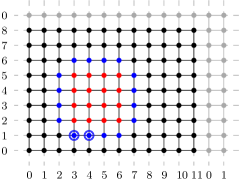
Figure 3: Toroidal rectangular grid graph of size $12\times 9$.

For showing that the up/down Markov chain on $2$-heights or $3$-heights of $G$ is rapidly mixing, we use the family $\mathcal{B}$ consisting of all contiguous $4\times 4$ blocks. In Figure 3, such a block is highlighted in red. Assuming that $g,h$ are sufficiently large, there are exactly $\lvert\mathcal{B}\rvert=g\cdot h$ such blocks, each vertex is contained in exactly $16$ blocks and forms part of $16$ block boundaries. Aiming for an application of Corollary 1, we have to bound the block divergence. We do this on the basis of of massive computations.

The boundary $\partial B$ consists of four paths of length $4$ (blue vertices in Figure 3). In every boundary constraint $X\in\Omega_{\partial B}$, the values of two successive vertices on one of these paths can differ by at most $1$. Further, in an extensible boundary constraint, the values of the last vertex of one path and the first vertex of the next path differ by at most $2$, because otherwise there is no possible value for the vertex in the corner of $B$.

If we consider the boundary as a chain of $16$ transitions, we can compute the number of the extensible boundary constraints as

$$\operatorname{tr}(Q_{k}P_{k}^{3}Q_{k}P_{k}^{3}Q_{k}P_{k}^{3}Q_{k}P_{k}^{3})=\operatorname{tr}\left((Q_{k}P_{k}^{3})^{4}\right),$$

where $P_{k}$ and $Q_{k}$ are both matrices of size $k\times k$ with

$$(P_{k})_{i,j}:=\begin{cases}1&\text{if }\lvert i-j\rvert\leq 1\\ 0&\text{otherwise}\end{cases}\text{ \hskip 31.2982pt }(Q_{k})_{i,j}:=\begin{cases}1&\text{if }\lvert i-j\rvert\leq 2\\ 0&\text{otherwise}\end{cases}.$$

If $k=2$ this gives $2.825.761$ extensible boundary constraints; if $k=3$ we get $15.784.802$ extensible boundary constraints. For any block $B\in\mathcal{B}$ and $v\in\partial B$, when we want to compute $E_{B,v}$, Lemma 2 tells us that this is the maximum of $\mathbb{E}[w(u)]-\mathbb{E}[w(\ell)]$ with random admissible fillings $\ell\sim\mathcal{U}(\Omega_{B|X})$ and $u\sim\mathcal{U}(\Omega_{B|Y})$ for two $k$-heights $X,Y$ that differ in a single vertex $v\in\partial B$, $X(v)=Y(v)-1$. For symmetry reasons, it is sufficient for the maximization to compute $E_{B,v}$ for the two vertices $v\in\partial B$ which are encircled in Figure 3.

Given a boundary constraint $X\in\Omega_{\partial B}$ we compute $\mathbb{E}[w(\ell)]$ for $\ell\sim\mathcal{U}(\Omega_{B|X})$ with a dynamic programming approach. For each row of the block we consider all the fillings consistent with the boundary conditions as vectors. By going from row to row we compute for each vector the number and total weight of all consistent assignments of vectors to previous rows. This then allows to compute the total weight $\sum_{\ell\in\Omega_{B|X}}w(\ell)$ of all admissible fillings and their number $\lvert\Omega_{B|X}\rvert$. The value of $\mathbb{E}[w(\ell)]$ is the quotient of the two numbers.

We do this computation for each boundary constraint $X\in\Omega_{\partial B}$ and store the result. Next, we iterate over all cover relations $X,Y\in\Omega_{\partial B}$ (up to symmetry) in order to compute $\max\{E_{B,v}:v\in\partial B\}$. The results are shown in Table 1. In the case $k=4$, we interrupted the execution but had already found a cover relation that gives the lower bound in the table.

$k$	$\max\{E_{B,v}:v\in\partial B\}$
$2$	$\approx 1.225092$
$3$	$\approx 1.752678$
$4$	$>2.27$

Table 1: Block divergence for blocks of size $4\times 4$ in rectangular grid.

Theorem 6.

Let $G=(V,E)$ be a toroidal rectangular grid graph, $n=\lvert V\rvert$. For $k\in\{2,3\}$ the up/down Markov-chain $\mathcal{M}$ operating on $k$-heights of $G$ is rapidly mixing. More precisely, the mixing time is upper bounded by

$$\tau(\varepsilon)<c_{k}\cdot\frac{\left(\left(\log(\frac{1}{\varepsilon})\cdot n\right)+n^{2}\cdot\log(k+1)\right)\cdot\log\left(\frac{kn}{\varepsilon}\right)}{\log(\frac{1}{2\varepsilon})}\in\mathcal{O}\left(n^{2}\log n\right),$$

where $c_{2}=2.844202\cdot 10^{10}$ and $c_{3}=1.333706\cdot 10^{13}$.

Proof.

In the notation of Corollary 1, for the family $\mathcal{B}$ of all contiguous blocks of size $4\times 4$ we have $\check{m}=s=16$. We obtain

$$1-\frac{1}{2\lvert\mathcal{B}\rvert}\left(\check{m}-s\cdot(E_{\text{max}}-1)\right)=:\beta_{k}<1$$

if and only if $E_{\text{max}}<2$. This holds for $k\in\{2,3\}$ as seen by the computational results in Table 1. Hence, Corollary 1 implies that the up/down Markov chain is rapidly mixing in these two cases and that the mixing times are upper bounded as in Theorem 1.

In the case $k=3$, we know $E_{\text{max}}<1.752678$, from which we get

$$\beta_{3}=1-\frac{1}{2\lvert\mathcal{B}\rvert}\left(\check{m}-s\cdot(E_{\text{max}}-1)\right)<1-\frac{1.978576}{\lvert\mathcal{B}\rvert},$$

and in the notation as in Theorem 1, using $b=m=16$, we obtain

$$c_{\mathcal{B},3}=\frac{8\cdot bmk(k+1)^{b}}{(1-\beta_{3})\lvert\mathcal{B}\rvert}<\frac{8\cdot bmk(k+1)^{b}}{1.978568}<1.333706\cdot 10^{13}.$$

In the case $k=2$, we do the same calculation based on $E_{\text{max}}<1.225093$ and obtain $c_{\mathcal{B},2}<2.844202\cdot 10^{10}$. ∎

For $k=4$ our computation shows $E_{\text{max}}>2$ (Table 1), which means that in Corollary 1 we cannot find such a $\beta_{4}<1$. We believe that the up/down Markov chain is rapidly mixing independently of $k$. We tried to use larger blocks for $\mathcal{B}$ but ran out of computational power.

4.2 $k$-heights on toroidal hexagonal grid graphs

For fixed $g,h\in\mathbb{N}$ we consider the triangular grid graph on $(\mathbb{Z}/g\mathbb{Z})\times(\mathbb{Z}/h\mathbb{Z})$, i.e., the vertices are points $(x,y)\in\mathbb{Z}\times\mathbb{Z}$ with horizontal edges $\left\{(x,y),(x+1,y)\right\}$, vertical edges $\left\{(x,y),(x,y+1)\right\}$ and diagonal edges $\left\{(x,y),(x+1,y+1)\right\}$, and we consider the $x$- and $y$-coordinates modulo $g$ and modulo $h$; respectively. Of the so obtained plane graph we take the dual graph $G$, whose vertices correspond to the $2\cdot g\cdot h$ triangular faces and edges in $G$ correspond to pairs of triangles that share a side; see Figure 4. The graph $G$ is a hexagonal grid.

(a)

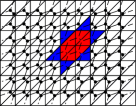
(b)

Figure 4: Hexagonal grid (a) or dual (b) of toroidal triangle grid of size $10\times 8$. Red vertices or faces form a block; blue vertices or faces are part of the boundary $\partial B$.

Every point $(x,y)\in\mathbb{Z}\times\mathbb{Z}$ defines a block $B_{x,y}$ consisting of $6$ vertices that correspond to the triangular faces incident to the vertex $(x,y)$; one such block is indicated in red in Figure 4. We use the family $\mathcal{B}:=\{B_{x,y}:x,y\in\mathbb{Z}\}$, which for sufficiently large $g,h$ has $g\cdot h$ blocks, each vertex is contained in $3$ blocks and $3$ block boundaries. Using the matrix $P_{k}$ defined in Section 4.1, we can compute the number of $k$-heights on a block as $\lvert\Omega_{B}\rvert=\operatorname{tr}(P_{k}^{6})$.

For every block $B$, the boundary $\partial B$ consists of $6$ isolated vertices. Therefore, there are exactly $\lvert\Omega_{\partial B}\rvert=(k+1)^{6}$ legal boundary constraints. If $k\geq 4$, some of them are not extensible, hence we could skip them in our computation. We iterated over all boundary constraints $\Omega_{\partial B}$ and fillings $\Omega_{B}$, as their cardinalities are small; see Table 2. The computation detects non extensible boundary constraints and simply ignores them. For symmetry reasons, when computing $\mathbb{E}[w(u)]-\mathbb{E}[w(\ell)]$ where $\ell\sim\mathcal{U}(\Omega_{B|X})$ and $u\sim\mathcal{U}(\Omega_{B|Y})$, we only need to do this for cover relations $(X,Y)$ on $\partial B$ that differ in a fixed vertex $v\in\partial B$.

$k$	$\lvert\Omega_{B}\rvert$	$\lvert\Omega_{\partial B}\rvert$	$\max\{E_{B,v}:v\in\partial B\}$
$2$	199	729	$\approx$ 0.798658
$3$	340	4096	$\approx$ 1.831905
$4$	481	15625	$\approx$ 2.892857
$5$	622	46656	3.0
$6$	763	117649	3.0

Table 2: Block divergence for blocks of $6$ hexagonal shaped vertices.

Theorem 7.

Let $G=(V,E)$ be a toroidal hexagonal grid graph, $n=\lvert V\rvert$. For $k\in\{2,3\}$ the up/down Markov-chain $\mathcal{M}$ operating on $k$-heights of $G$ is rapidly mixing. More precisely, the mixing time is upper bounded by

$$\tau(\varepsilon)<c_{k}\cdot\frac{\left(\left(\log(\frac{1}{\varepsilon})\cdot n\right)+n^{2}\cdot\log(k+1)\right)\cdot\log\left(\frac{kn}{\varepsilon}\right)}{\log(\frac{1}{2\varepsilon})}\in\mathcal{O}\left(n^{2}\log n\right),$$

where $c_{2}=1.165099\cdot 10^{5}$ and $c_{3}=7.017788\cdot 10^{6}$.

Proof.

In the notation of Corollary 1, for the family of blocks $\mathcal{B}$ that we have described above we have $\check{m}=s=3$. We obtain

$$1-\frac{1}{2\lvert\mathcal{B}\rvert}\left(\check{m}-s\cdot(E_{\text{max}}-1)\right)=:\beta_{k}<1$$

if and only if $E_{\text{max}}<2$. This holds for $k\in\{2,3\}$ as seen by the computational results in Table 1. Hence, Corollary 1 implies that the up/down Markov chain is rapidly mixing in these two cases and that the mixing times are upper bounded as in Theorem 1.

In the case $k=3$, we know $E_{\text{max}}<1.831906$, from which we get

$$\beta_{3}=1-\frac{1}{2\lvert\mathcal{B}\rvert}\left(\check{m}-s\cdot(E_{\text{max}}-1)\right)<1-\frac{0.252141}{\lvert\mathcal{B}\rvert},$$

and in the notation as in Theorem 1, using $b=6$ and $m=3$ we obtain

$$c_{\mathcal{B},3}=\frac{8\cdot bmk(k+1)^{b}}{(1-\beta_{3})\lvert\mathcal{B}\rvert}<\frac{8\cdot bmk(k+1)^{b}}{0.252141}<7.017788\cdot 10^{6}.$$

In the case $k=2$, we do the same calculation based on $E_{\text{max}}<0.798659$ and obtain the bound $c_{\mathcal{B},2}<1.165099\cdot 10^{5}$. ∎

Again, for $k=4$ our computation shows $E_{\text{max}}>2$ (Table 2), which means that in Corollary 1 we cannot find such a $\beta_{4}<1$.

4.3 $k$-heights on planar $3$-regular graphs

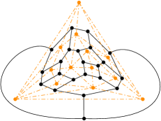
Figure 5: Example of a dual graph (black, solid) of a $4$-connected triangulation (orange, dashed)

Theorem 8.

Let $G=(V,E)$ be a simple $2$-connected $3$-regular planar graph, and let $n=\lvert V\rvert$.

• The mixing time $\tau(\varepsilon)$ of the up/down Markov chain $\mathcal{M}$ operating on $2$-heights is upper bounded by

  $$\tau(\varepsilon)<c_{k}\cdot\frac{\left(\left(\log(\frac{1}{\varepsilon})\cdot n\right)+n^{2}\cdot\log(k+1)\right)\cdot\log\left(\frac{kn}{\varepsilon}\right)}{\log(\frac{1}{2\varepsilon})}\in\mathcal{O}\left(n^{2}\log n\right)\;,$$

  where $c_{2}=4.391132\cdot 10^{7}$.

• If $G$ is even $3$-connected, then, for $k\in\{2,3\}$, the mixing time $\tau(\varepsilon)$ of the up/down Markov chain $\mathcal{M}$ operating on $k$-heights is upper bounded by the same expression as in (1) with constants $c_{2}=2.195097\cdot 10^{7}$ and $c_{3}=4.852027\cdot 10^{9}$.

• If $G$ is the dual graph of a $4$-connected triangulation, then, for $k\in\{2,3\}$, the mixing time $\tau(\varepsilon)$ of the up/down Markov chain $\mathcal{M}$ operating on $k$-heights is upper bounded by the same expression as in (1) with constants $c_{2}=1.489256\cdot 10^{7}$ and $c_{3}=4.852027\cdot 10^{9}$.

For a fixed plane embedding of $G$ we construct a family $\mathcal{B}$ of blocks of the following two types. For every face $F$ of degree $d\leq 10$ we consider the block consisting of all $d$ boundary vertices and call it a block of type $1$, or, more specifically, a block of type $1_{d}$; see Figure 6(a). In $\mathcal{B}$ we include $8$ identical copies of each such block. For every face $F$ of degree $d>10$, we consider all sets of $8$ successive vertices on the boundary of $F$ and call them blocks of type $2$. We include each of these $d$ blocks (a single time) in $\mathcal{B}$; see Figure 6(b) for an example.

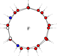
(a)

(b)

Figure 6: Red vertices form a block of type $1_{9}$ in (a) and a block of type $2$ in (b). Blue vertices are part of the boundary $\partial B$.

As a first consequence of this construction, each vertex $v$ is contained in exactly $24$ blocks in $\mathcal{B}$: As $\operatorname{deg}(v)=3$ and $G$ is $2$-connected, vertex $v$ belongs to $3$ distinct faces, each of which contributes $8$ blocks containing $v$.

When computing the block divergence $E_{B,v}$ for some $v\in\partial B$, we distinguish different cases depending on the type of $B$ and the adjacency relations between $B$ and $v$. If $B$ is of type $1_{d}$, we label the vertices in clockwise order around $F$ as $1,\ldots,d$. In fact, due to symmetry, it will not be relevant at which vertex the numbering starts. If $B$ is of type $2$, we label its vertices in clockwise order as $1,\ldots,8$.

Note that $v\in\partial B$ can be adjacent to one, two or three vertices of $B$. The cases in the following case distinction will be tagged by the type of $B$ followed by the labels of the neighbors of $v$ in square brackets. For instance, Case $1_{5}[1]$ describes the scenario in which $v$ is adjacent to a single vertex of a block of type $1_{5}$. Due to symmetry, the cases $1_{5}[x]$ with $x\in\{1,\ldots,5\}$ are all equivalent to Case $1_{5}[1]$; they result in the same block divergence $E_{B,v}$. As another example, Figure 7 shows Case $2[2,5]$, i.e., $v$ is adjacent to vertices $2$ and $5$ of a block of type $2$. This case is symmetrical to Case $2[4,7]$, both result in the same block divergence $E_{B,v}$.

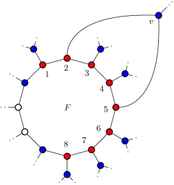
Figure 7: Case $2[2,5]$: Vertex $v$ is adjacent to vertices $2$ and $5$ from a block $B$ which is of type $2$. The block divergence $E_{B,v}$ is the same as in Case $2[4,7]$.

In a block $B$ of type $2$, vertices $1$ and $8$ have two neighbors in $\partial B$. Note that when $v$ is one of these two neighbors, our tag will not tell whether $v$ belongs to the boundary of $F$. This information would not affect $E_{B,v}$.

Further, note that for a block $B$ of any type, so far we did not consider the cases in which some boundary vertex other than $v$ is adjacent to multiple vertices in $B$. For instance, in the example in Figure 7, vertices $3$ and $4$ or some of the vertices $1$, $6$, $7$, $8$ could be adjacent to a common boundary vertex. However, these cases are already covered in our computation of $E_{B,v}$, where we consider all boundary constraints $\Omega_{\partial B}$, including those where some of the boundary vertices are assigned the same value. Hence, these further cases can only have a smaller block divergence.

For $k=2$ and $k=3$, we used a computer program to compute $E_{B,v}$ for all cases described above; see Table 3 for cases where $B$ is of type $1$ and Table 4 for cases where $B$ is of type $2$. Whenever multiple cases result in the same block divergence $E_{B,v}$ for symmetry reasons, the tables contain only one of them.

It turns out that in this setting Corollary 1 is not strong enough for proving that $\mathcal{M}$ is rapidly mixing: Each vertex is contained in exactly $\check{m}=24$ blocks and in at most $s=30$ boundaries of blocks; and even in the case $k=2$ we have $E_{\textup{max}}\approx 2.367241$ (with Case $1_{10}[1,3,7]$ being the extremal case; see Table 3 and Table 4), which gives $m-s(E_{\text{max}}-1)<-17.0172<0$. Therefore, instead of applying Corollary 1, we will apply Theorem 1 directly.

Lemma 6.

If $G=(V,E)$ is a simple $2$-connected $3$-regular planar graph, then, with the family $\mathcal{B}$ of blocks described above and $k=2$, we have

$$\#\{B\in\mathcal{B}\;\mid\;v\in B\}\hskip 5.69046pt-\sum_{B\in\mathcal{B}\;\mid\;v\in\partial B}(E_{B,v}-1)\hskip 2.84544pt>\hskip 2.84544pt10.32755$$

for all $v\in V$.

Proof.

We have already observed $\#\left\{B\in\mathcal{B}\;\mid\;v\in B\right\}=24$. For analysing the sum on the right hand side, we have to consider all blocks $B\in\mathcal{B}$ with $v\in\partial B$ and look up the corresponding cases in Table 3 and Table 4. As $v$ has degree $3$ and $G$ is $2$-connected, $v$ is incident to exactly three pairwise distinct faces $H_{1}$, $H_{2}$ and $H_{3}$. Its three neighbors $w_{1}$, $w_{2}$ and $w_{3}$ are incident to three further faces $F_{1}$, $F_{2}$ and $F3$, as shown in Figure 8.

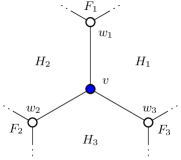
Figure 8: A vertex $v$ can only be in the boundary of a block induced from any of the faces $H_{1}$, $H_{2}$, $H_{3}$, $F_{1}$, $F_{2}$ and $F_{3}$.

There are at most $30$ blocks $B\in\mathcal{B}$ with $v\in\partial B$: At most $8$ induced by each of the faces $F_{1}$, $F_{2}$ and $F_{3}$, and at most $2$ induced by each of the faces $H_{1}$, $H_{2}$ and $H_{3}$.

In the case in which the faces $H_{1}$, $H_{2}$, $H_{3}$, $F_{1}$, $F_{2}$, $F_{3}$ are pairwise distinct, every block $B\in\mathcal{B}$ contains at most one vertex adjacent to $v$. In the corresponding cases in Table 3 and Table 4, we have $E_{B,v}<0.80456$, with $1_{10}[1]$ being the extremal case. Moreover, there are at least $24$ blocks $B\in\mathcal{B}$ with $v\in\partial B$, namely the $8$ blocks induced by each of the faces $F_{1}$, $F_{2}$ and $F_{3}$. From this we directly get

$$\#\{B\in\mathcal{B}\;\mid\;v\in B\}\hskip 5.69046pt-\sum_{B\in\mathcal{B}\;\mid\;v\in\partial B}(E_{B,v}-1)\quad>\quad 24+24\cdot 0.19544\quad>\quad 28.$$

However, the faces $F_{1}$, $F_{2}$ and $F_{3}$ do not need to be pairwise distinct, and they can be identical to a face $H_{1}$, $H_{2}$ or $H_{3}$. In such cases, blocks may occur that contain two or three vertices adjacent to $v$, which requires a refined analysis.

From the data in Table 3 and Table 4 we get

$$E^{*}:=\max_{B\in\mathcal{B}\;\mid\;v\in\partial B}\hskip 5.69046pt\frac{E_{B,v}-1}{\#\left\{w\in B\;:\;\{v,w\}\in E\right\}}<0.455748,$$

with Case $1_{10}[1,3,7]$ being the extremal case. Now we have:

$$\sum_{B\in\mathcal{B}\;\mid\;v\in\partial B}E_{B,v}-1 =\sum_{B\in\mathcal{B}\;\mid\;v\in\partial B}\#\left\{w\in B:\{v,w\}\in E\right\}\frac{E_{B,v}-1}{\#\left\{w\in B:\{v,w\}\in E\right\}}$$

$$\leq\hskip 2.84544ptE^{*}\cdot\sum_{i=1}^{3}\#\left\{B\in\mathcal{B}:w_{i}\in B,v\notin B\right\}$$

$$<\hskip 2.84544pt0.455748\cdot 30=13.67245$$

In the last inequality we used that there are at most $10$ blocks $B\in\mathcal{B}$ with $w_{i}\in B$ and $v\notin B$: At most $8$ induced by $F_{i}$ and at most one induced by each of the two faces $H_{j}$ that are incident to $w_{i}$. Finally, we obtain

$$\#\{B\in\mathcal{B}\;\mid\;v\in B\}\hskip 5.69046pt-\sum_{B\in\mathcal{B}\;\mid\;v\in\partial B}(E_{B,v}-1)$$

$$>\hskip 5.69046pt24-13.67245\;=\;10.32755\hskip 2.84544pt.$$

∎

Lemma 7.

If $G=(V,E)$ is a $3$-connected $3$-regular planar graph, then, with the family $\mathcal{B}$ of blocks constructed above and in the case $k\in\{2,3\}$, we have

$$\#\{B\in\mathcal{B}\;\mid\;v\in B\}\hskip 5.69046pt-\sum_{B\in\mathcal{B}\;\mid\;v\in\partial B}(E_{B,v}-1)\hskip 2.84544pt>\hskip 2.84544pt\begin{cases}20.659512&k=2\\ 2.489598&k=3\end{cases}$$

for all $v\in V$.

Proof.

The proof is similar to the proof of Lemma 6, but the $3$-connectivity allows us to exclude cases that would imply a $2$-separator. For instance, in Case $2[2,5]$, depicted in Figure 7, the vertices $2$ and $5$ form a $2$-separator, hence, it cannot occur in $G$. Indeed, we can exclude all cases in which $v$ is adjacent to two non-consecutive vertices on $B$ (For example, Case $2[2,5]$) or adjacent to three vertices on $B$ (For example, Case $2[2,4,5]$). The remaining cases are those in which $v$ has only one neighbor in $B$ (For example, Case $2[3]$) or exactly two neighbors that lie consecutively on $B$ (For example, Case $2[3,4]$).

First, we treat the case $k=3$. For upper bounding $E^{*}$ as in the proof of Lemma 6, we maximize over the cases that we did not exclude. Using the values from Table 3 and Table 4, we obtain $E^{*}<0.848707$ with Case $1_{10}[1]$ being the extremal case.

Recall the notation from Figure 8. From the $3$-connectivity of $G$ it follows that each of the faces $F_{1}$, $F_{2}$ and $F_{3}$ is distinct to the faces $\{H_{1},H_{2},H_{3}\}$: Clearly, $F_{1}$ is distinct to $H_{1}$ and $H_{2}$, since otherwise, the vertex $w_{1}$ would be a separator. Further, $F_{1}$ is distinct to $H_{3}$, as otherwise, the vertices $\{v,w_{1}\}$ would separate $w_{3}$ from $w_{2}$. The statement for $F_{2}$ and $F_{3}$ follows by symmetry.

Let $\mathcal{B}_{F}\subset\mathcal{B}$ be the set of blocks that are induced by the faces $\{F_{1},F_{2},F_{3}\}$, and let $\mathcal{B}_{H}\subset\mathcal{B}$ be the set of blocks that are induced by the faces $\{H_{1},H_{2},H_{3}\}$. Using the fact that $\{H_{1},H_{2},H_{3}\}$ are distinct from $\{F_{1},F_{2},F_{3}\}$, we can get the following: The only way in which $v$ can be in the boundary of a block $B$ induced by $H_{i}$ is when $H_{i}$ has degree larger than $10$ and $B$ is of type $2$ consisting of the $8$ consecutive vertices either before or behind $v$ on the boundary of $H_{i}$. These are Case $2[8]$ and Case $2[1]$, which lead to the same block divergence $E_{B,v}\approx 1.190238$; see Table 4.

This allows us to refine the analysis that we already did in the proof of Lemma 6:

$$\sum_{B\in\mathcal{B}\;\mid\;v\in\partial B}E_{B,v}-1$$

$$=\left(\sum_{B\in\mathcal{B}_{H}\;\mid\;v\in\partial B}E_{B,v}-1\right)+\left(\sum_{B\in\mathcal{B}_{F}\;\mid\;v\in\partial B}E_{B,v}-1\right)$$

$$<\hskip 2.84544pt6\cdot(1.190239-1)+E^{*}\cdot\sum_{i=1}^{3}\#\left\{B\in\mathcal{B}_{F}:w_{i}\in B,v\notin B\right\}$$

$$<\hskip 2.84544pt6\cdot 0.190239+0.848707\cdot 24=21.510402$$

From this we obtain our result for the case $k=3$:

$$\#\{B\in\mathcal{B}\;\mid\;v\in B\}\hskip 5.69046pt-\sum_{B\in\mathcal{B}\;\mid\;v\in\partial B}(E_{B,v}-1)$$

$$>\hskip 5.69046pt24-21.510402\;=\;2.489598$$

The result for $k=2$ is obtained using the very same calculations. From Table 3 and Table 4 we get $E^{*}<0.212547$ (with Case $1_{10}[1,2]$ being the extremal case), for Case 2[8] and Case 2[1] we have $E_{B,v}\approx 0.706599$ and obtain

$$\#\{B\in\mathcal{B}\;\mid\;v\in B\}\hskip 5.69046pt-\sum_{B\in\mathcal{B}\;\mid\;v\in\partial B}(E_{B,v}-1)$$

$$>\hskip 5.69046pt24-(6\cdot(0.706560-1)+0.212547\cdot 24)\;=\;20.659512$$

∎

Lemma 8.

If $G=(V,E)$ is the dual graph of a $4$-connected triangulation, then, with the family $\mathcal{B}$ of blocks constructed above and in the case $k\in\{2,3\}$, we have

$$\#\{B\in\mathcal{B}\;\mid\;v\in B\}\hskip 5.69046pt-\sum_{B\in\mathcal{B}\;\mid\;v\in\partial B}(E_{B,v}-1)\hskip 2.84544pt>\hskip 2.84544pt\begin{cases}30.4512&k=2\\ 2.489598&k=3\end{cases}$$

for all $v\in V$.

Proof.

We know that $G$ is $3$-connected as the dual of a $4$-connected triangulation, so we could directly refer to Lemma 7. However, the fact that $G$ is the dual of a $4$-connected triangulation allows to exclude further cases, namely all cases in which $v$ has more than one neighbor in $B$. Apart from this further restriction, the proof is exactly the same. We just mention the relevant data: From Table 3 and Table 4 we get for $k=2$ the bound $E^{*}<-0.195440$ and for $k=3$ the bound $E^{*}<0.848707$ (with Case $1_{10}[1]$ being the extremal case for both $k\in\{2,3\}$). ∎

Proof of Theorem 8.

We apply Theorem 1. In the case of planar $2$-heights on $2$-connected $3$-regular graphs, by Lemma 6, we have

$$\beta_{2} :=1-\frac{1}{2\lvert\mathcal{B}\rvert}\left(\#\{B\in\mathcal{B}\;\mid\;v\in B\}\hskip 5.69046pt-\sum_{B\in\mathcal{B}\;\mid\;v\in\partial B}(E_{B,v}-1)\right)$$

$$<\hskip 2.84544pt1-\frac{5.163775}{\lvert\mathcal{B}\rvert},$$

and in the notation as in Theorem 1, using $b=10$ and $m=24$, we obtain

$$c_{\mathcal{B},2}=\frac{8\cdot bmk(k+1)^{b}}{(1-\beta_{2})\lvert\mathcal{B}\rvert}<\frac{8\cdot bmk(k+1)^{b}}{5.163775}<4.391132\cdot 10^{7}.$$

Part (2) and (3) follow using the same calculation and Lemma 7 and Lemma 8. ∎

5 Glauber dynamics

A spin system consists of a graph $G=(V,E)$, where the vertices $V$ are also called sites, a finite set $Q=\{1,\ldots,q\}$ of possible spins and a set of feasible configurations $\Omega\subset Q^{V}$, where $Q^{V}:=\{\varphi:V\to Q\}$. Examples include proper $q$-colorings, independent sets (hardcore model) and magnetic states (Ising model); see [3], from which we take the following notation.

Spin systems are inspired by physics; in a configuration $\varphi\in Q^{V}$ there are interacting forces between neighbor sites depending on their spins, making some of the configurations less likely or infeasible. This is expressed by a weight or "inverse energy" function $w:Q^{V}\to\mathbb{R}_{\geq 0}$,

$$w(\varphi)=\prod_{\{v,w\}\in E}A_{vw}(\varphi(v),\varphi(w))\hskip 5.69046pt\prod_{v\in V}B_{v}(\varphi(v))\;,$$

where $A_{vw}:Q\times Q\to\mathbb{R}_{\geq 0}$ are symmetric functions that represent the interaction between any two neighbor sites, and $B_{v}:Q\to\mathbb{R}_{\geq 0}$ measures the influence of an "external field" on $v$. Then, typically, one chooses $\Omega:=\{\varphi\in Q^{V}:w(\varphi)>0\}$. The Gibbs distribution $\mu$ is the probability distribution on $\Omega$ in which the probability of an element $\varphi$ is proportional to its weight, i.e., $\mu(\varphi)=w(\varphi)/Z_{w}$, where $Z_{w}=\sum_{\phi\in\Omega}w(\phi)$.

In general, sampling from $\mu$ is hard; in most cases, computing $Z_{w}$ is already as hard as counting $\Omega$. This is where Glauber dynamics come into play. These are Markov chains $(\varphi_{t})$ that operate on $\Omega$ an converge towards $\mu$. In each step, they randomly select a site $v$ (or traverse all sites in some order) and randomly update its spin $\varphi_{t}(v)$ according to a distribution $\nu_{\varphi_{t},v}:Q\to[0,1]$, which is called update rule. A remarkable result due to Hayes and Sinclair [14] is that for any Glauber dynamics that is based on a local and reversible update rule, $\Omega(n\log n)$ is a lower bound on the mixing time on graphs of bounded degree. Local means that $\nu_{\varphi,v}$ may only depend on the current spins of $v$ and its neighbors. An update rule is reversible if $\mu(\varphi)\cdot\nu_{\varphi,v}(q^{\prime})=\mu(\varphi^{\prime})\cdot\nu_{\varphi^{\prime}\kern-2.0pt,v}(q)$ whenever $\varphi(v)=q$ and $\varphi^{\prime}$ is obtained from $\varphi$ by changing the spin at $v$ to $q^{\prime}$.

Clearly, by setting $Q=\{0,\ldots,k\}$ and with

$$A_{vw}(q_{1},q_{2}):=\begin{cases}1&\text{if }\lvert q_{1}-q_{2}\rvert\leq 1\\ 0&\text{otherwise}\end{cases}\;,\text{ \hskip 19.91684pt }B_{v}:\equiv 1\;,$$

the set of feasible configurations $\Omega$ coincides exactly with the set of $k$-heights, each element has the same weight, and hence, the Gibbs distribution equals the uniform distribution $\mathcal{U}(\Omega)$. The up/down Markov chain $\mathcal{M}=(X_{t})$ selects in each iteration uniformly a site $v$ and updates its spin $X_{t}(v)$ depending on a coin flip and depending on the spins of the neighbors of $v$. Clearly, this up/down update rule is local and also symmetric, hence reversible. This implies an $\Omega(n\log n)$ lower bound on its mixing time for all classes of graphs that we studied in Section 4, because their vertex degree is bounded.

In [3] they study heat-bath update rules and conditions that imply that the asymptotic lower bound is tight, i.e., the mixing time is $\Theta(n\log n)$. An update rule is a heat-bath update rule, if the updated spin for $v$ is sampled according to $\mu$ conditioned on the spins of all other vertices; more precisely,

$$\nu_{\varphi,v}(q)=\operatorname{Prob}_{\mu}[\phi(v)=q\;|\;\phi(w)=\varphi(w)\text{ for all }w\neq v]\;.$$

It is easy to see that the heat-bath update rule coincides exactly with the block Markov chain $\mathcal{M}_{\mathcal{B}}$ for a family of singleton blocks $\mathcal{B}=\left\{\{v\}\;:\;v\in V\right\}$. In fact, the authors in [3] also generalize their results to so called block dynamics, i.e., to resampling larger blocks, just as $\mathcal{M}_{\mathcal{B}}$ does.

Theorem 9 (Blanca et al., Theorem 1.6 in [3]).

For an arbirary spin system on a graph of maximum degree $\Delta$, if the system is $\eta$-spectrally independent and $b$-marginally bounded, then there exists a constant $C=C(b,\eta,\Delta)$ such that the mixing time of the Glauber dynamics is upper bounded by $\tau(\varepsilon)<C\cdot n\log n$, where $C=\left(\frac{\Delta}{b}\right)^{\mathcal{O}(1+\frac{\eta}{b})}$.

With the next lemma we show that the spin system of $k$-heights is $b$-marginally bounded. After that we comment on the other condition of Theorem 9: spectral independence.

Recall the definitions of $\Omega_{B}$ and $\Omega_{B|X}$ in Subsection 2.3. They naturally generalize to spin systems other than $k$-heights. Let $\mu_{B|X}$ denote the distribution on $\Omega_{B|X}$ which is the Gibbs distribution conditioned on the spin values of $X$ in the set $V\setminus B$. In the case of $k$-heights, $\mu_{B|X}=\mathcal{U}(\Omega_{B})$. A spin system is called $b$-marginally bounded, if for every $X\in\Omega$, for every $B\subset V$, for every site $v\in B$ and for any spin $q$ for which there exists a $\varphi\in\Omega_{B|X}$ with $\varphi(v)=q$, the probability under $\mu_{B|X}$ of seeing spin $q$ at site $v$ is lower bounded by $b$, i.e., $\operatorname{Prob}_{\mu_{B|X}}[\phi(v)=q]\geq b$.

In a graph $G$ we let $B_{r}(v):=\{w\in V:\operatorname{dist}(v,w)<r\}\hskip 2.84544pt$ be the ball of radius $r$ around $v$.

Lemma 9.

With respect to the spin system of $k$-heights on $G$, the Gibbs distribution $\mu=\mathcal{U}(\Omega)$ is $b$-marginally bounded with

$$b:=\frac{1}{(k+1)^{(\Delta-1)^{k-1}}}\;,$$

where $\Delta$ denotes the maximum degree of $G$.

Proof.

Fix $X\in\Omega$, a set $B\subset V$, a site $v\in B$ and spin $q\in Q$. Define $k$-heights $L,U\in\Omega_{B}$ by

$$L(w) :=\max\{q-\operatorname{dist}(v,w),0\}$$

$$U(w) :=\min\{q+\operatorname{dist}(v,w),k\}$$

for any $w\in B$, where $\operatorname{dist}(v,w)=\infty$ if there is no $v-w$ path in $B$. Let

$$f:\Omega_{B}\to\Omega_{B},\hskip 14.22636ptY\mapsto(Y\lor U)\land L\;,$$

where $\lor$ resp. $\land$ denotes the pointwise minimum resp. maximum of two $k$-heights. Indeed, $f$ is well defined, as $\Omega_{B}$ is closed under these operations. Note that $f(Y)(v)=q$, and $Y$ and $f(Y)$ can only differ on sites in the ball $B_{k}(v)$.

We will now show that $Y\in\Omega_{B|X}$ implies $f(Y)\in\Omega_{B|X}$. Let $(w,w^{\prime})$ be an edge with $w\in B$ and $w^{\prime}\not\in B$, i.e., $w^{\prime}\in\partial B$. The claim is that $X(w^{\prime})-1\leq f(Y)(w)\leq X(w^{\prime})+1$. By assumption, there exists $\varphi\in\Omega_{B|X}$ with $\varphi(v)=q$. We know $\varphi(w)\geq q-\operatorname{dist}(v,w)$ by the $k$-height property, hence, $L(w)\leq\varphi(w)\leq X(w^{\prime})+1$. Since $Y\in\Omega_{B|X}$ we have $Y(w)\leq X(w^{\prime})+1$, and we obtain

$$f(Y)(w) =((Y\lor U)\land L)(w)\leq(L\land Y)(w)$$

$$=\max\{L(w),Y(w)\}\leq X(w^{\prime})+1\;.$$

A similar argument shows $f(Y)(w)\geq X(w^{\prime})-1$: first show that $Y(w)$ and $U(w)$ and hence also $(Y\lor U)(w)$ are lower bounded by $X(w^{\prime})-1$, therefore, $X(w^{\prime})-1$ is also a lower bound for the pointwise maximum $((Y\lor U)\land L)(w)=f(Y)(w)$. This completes the proof of $f(Y)\in\Omega_{B|X}$.

Let $W:=B\setminus B_{k}(v)$. For an admissible filling $\varphi\in\Omega_{B|X}$, let ${\left.\kern-1.2pt\varphi\mathchoice{\vphantom{\big{|}}}{}{}{}\right|_{W}}\in\Omega_{W}$ be the restriction on $W$ and let $\Omega_{W}^{*}:=\{\phi\in\Omega_{W}\;|\;\exists\varphi\in\Omega_{B|X}:{\left.\kern-1.2pt\varphi\mathchoice{\vphantom{\big{|}}}{}{}{}\right|_{W}}=\phi\}$. By definition, every $\phi\in\Omega_{W}^{*}$ can be extended to an admissible filling $\varphi\in\Omega_{B|X}$, but by applying $f$ on any such extension, it can be even extended to an admissible filling $\varphi\in\Omega_{B|X}$ with $\varphi(v)=q$. In other words, out of at most

$$(k+1)^{\lvert B\cap B_{k}(x)\rvert}\leq(k+1)^{\lvert B_{k}(x)\rvert}\leq(k+1)^{(\Delta-1)^{k-1}}=b^{-1}$$

ways to extend $\phi\in\Omega_{W}^{*}$ to an admissible filling $\varphi\in\Omega_{B|X}$, there exists at least one which fulfills $\varphi(v)=q$. For a random admissible filling $\varphi\sim\mathcal{U}(\Omega_{B|X})$ we conclude:

$$\operatorname{Prob}[\varphi(v)=q]\geq b\;.$$

∎

The second condition of Theorem 9 requires the spin system to be $\eta$-spectrally independent. This is defined in [3] in terms of the ALO influence matrix. Let $B\subset V$, $X\in\Omega$, let $T=V\times Q$ and let $J_{B|X}\in\mathbb{R}^{\mathcal{T}\times\mathcal{T}}$ be the ALO influence matrix defined as

$$J_{B|X}(v,q,v^{\prime},q^{\prime}):=\operatorname{Prob}_{\mu_{B|X}}[\varphi(v)=q\;|\;\varphi(v^{\prime})=q^{\prime}]-\operatorname{Prob}_{\mu_{B|X}}[\varphi(v)=q]\;.$$

Now, the spin system is said to be $\eta$-spectrally independent if for all $B\subset V$ and $X\in\Omega$ the largest eigenvalue $\lambda_{1}$ of $J_{B|X}$ satisfies $\lambda_{1}<\eta$.

Blanca et al. [3] relate $\eta$-spectral independence with the existence of contracting couplings as in Theorem 2. Let $U\subset V$. For a so called pinning $\tau:U\to Q$, the restricted Glauber dynamics $(\varphi_{t}^{\tau})$ operates on the set $\Omega_{V\setminus U|\tau}$; in each step it updates a site in $V\setminus U$ using the heat bath update rule w.r.t. the distribution $\mu_{V\setminus U|\tau}$. They prove the following result:

Theorem 10 (Blanca et al., Theorem 1.10 in [3]).

If for every pinning $\tau:U\to Q$ there is a coupling $(X_{t},Y_{t})$ of the restricted Glauber dynamics $(\phi_{t}^{\tau})$ and a $\beta<1$ such that

$$\mathbb{E}[d(X_{t+1},Y_{t+1})]<\beta\cdot d(X_{t},Y_{t})\;,$$

where $d(X,Y):=\#\{v\in\Omega_{V\setminus U}:X(v)\neq Y(v)\}$, then the spin system is $\eta$-spectrally independent with constant $\eta=\frac{2}{(1-\beta)n}$.

This result can be extended to block dynamics operating on $\Omega_{V\setminus U|\tau}$ using an arbitrary family of blocks $\mathcal{B}\subset\mathcal{P}(V\setminus U)$; see Theorem 1.11 in [3]. Under the conditions of Theorem 1 the block coupling that we constructed in Algorithm 3 is a contracting coupling as required by Theorem 10 in the absence of any pinning ($U=\emptyset$). However, it seems difficult for us to establish a contracting block coupling that is compatible with the restriction under an arbitrary pinning $\tau:U\to V$.

We leave it as an open question in which cases the spin system of $k$-heights satisfies $\eta$-spectral independence. This would imply an optimal mixing time of $\Theta(n\log n)$ for $\mathcal{M}_{\mathcal{B}}$ using singleton blocks $\mathcal{B}=\left\{\{v\}\;:\;v\in V\right\}$.

6 Conclusion

In this work we studied a natural up/down Markov chain $\mathcal{M}$ operating on $k$-heights, which can also be considered as valid configurations $\sigma:V\to\{0,\cdots,k\}$ of a spin systems with hard constraints $\lvert\sigma(v)-\sigma(w)\rvert\leq 1$ for all $\{v,w\}\in E$. We established a criterion for the boosted block Markov chain $\mathcal{M}_{\mathcal{B}}$ to be rapidly mixing, which implies that $\mathcal{M}$ is rapidly mixing as well, and showed several examples of graph classes to which it applies.

Question 1.

Is the up/down Markov chain $\mathcal{M}$ on the graph classes discussed in Theorem 6, Theorem 7 and Theorem 8 rapidly mixing for all values of $k$?

For some smaller values of $k$, using larger blocks $\mathcal{B}$ and more computational power, one might be able to show that Theorem 1 can still be applied, hence, $\mathcal{M}$ mixes rapidly. A completely affirmative answer of Question 1, i.e. for arbitrary large values of $k$, could consist of an argument which guarantees that one can always choose the blocks large enough so that the conditions of Theorem 1 are satisfied.

Intuitively, for a vertex $v\in\partial B$ and a vertex $w\in B$ with large distance $\operatorname{dist}(v,w)$, an increase of $X(v)$ should not greatly affect the distribution of $X^{\prime}(w)$ when $X^{\prime}\sim\mathcal{U}(\Omega_{B|X})$. This intuition is captured by the concept of spatial mixing. The spin system of $k$-heights has strong spatial mixing, if there exist constants $\beta$ and $\alpha>0$ so that for all $B^{\prime}\subset B\subset V$ and for any pair of boundary constraints $X,Y\in\partial B$ that differ only in a single vertex $v\in\partial B$ we have

$$\lVert\mathcal{U}(\Omega_{B|X})-\mathcal{U}(\Omega_{B|Y})\rVert_{B^{\prime}}<\beta\cdot\lvert B^{\prime}\rvert\cdot\operatorname{exp}(-\alpha\cdot\operatorname{dist}(v,B^{\prime}))\;,$$

where $\lVert\mu-\mu^{\prime}\rVert_{B^{\prime}}$ denotes the total variation distance of the projections of $\mu,\mu^{\prime}$ on $B^{\prime}$. Dyer, Sinclair, Vigoda and Weitz [9] have shown that spatial mixing implies a mixing time of $\mathcal{O}(n\log n)$ if the system is monotone. In fact, the system of $k$-heights is monotone by Proposition 1. Hence, the following question becomes relevant:

Question 2.

For which classes of graphs and for which values of $k$ does the system of $k$-heights have strong spatial mixing with respect to the uniform distribution?

Finally, we want to mention that $\mathcal{M}$ is clearly not rapidly mixing on any graph. The easiest example is the complete graph $K_{n}$ on $n$ vertices and $k=2$. There are three disjoint classes of $k$-heights which form a partition of $\Omega$:

$$\Omega_{>} :=\{X\in\Omega\;|\;\exists v\in V:X(v)=0\} \lvert\Omega_{>}\rvert =2^{n}-1$$

$$\Omega_{<} :=\{X\in\Omega\;|\;\exists v\in V:X(v)=2\} \lvert\Omega_{<}\rvert =2^{n}-1$$

$$\Omega_{=} :=\{X_{1}\equiv 1\} \lvert\Omega_{=}\rvert =1$$

Every sequence of transitions between $\Omega_{<}$ and $\Omega_{>}$ must contain $X_{1}$, and $X_{1}$ is incident to exactly $n$ transitions to each of the other two classes. Clearly, this is a bottleneck which shows that $\mathcal{M}$ is not rapidly mixing; see [20, Theorem 7.4].

Question 3.

Is the up/down Markov chain $\mathcal{M}$ on $k$-heights rapidly mixing on all graphs of maximum degree bounded by $\Delta$, for some or arbitrary values $\Delta\geq 2$?

Appendix A Block divergence on $3$-regular graphs

Table 3: Block divergence for blocks of type $1$.

$k$	Case	$\lvert\Omega_{B}\rvert$	$\lvert\Omega_{\partial B}\rvert$	$\max E_{B,v}$
2	$1_{3}[1]$	15	27	$\approx$ 0.727273
2	$1_{4}[1]$	35	81	$\approx$ 0.769231
2	$1_{5}[1]$	83	243	$\approx$ 0.790323
2	$1_{6}[1]$	199	729	$\approx$ 0.798658
2	$1_{7}[1]$	479	2187	$\approx$ 0.802228
2	$1_{8}[1]$	1155	6561	$\approx$ 0.803695
2	$1_{9}[1]$	2787	19683	$\approx$ 0.804306
2	$1_{10}[1]$	6727	59049	$\approx$ 0.804559
2	$1_{3}[1,2]$	15	9	$\approx$ 1.327273
2	$1_{4}[1,2]$	35	27	$\approx$ 1.384615
2	$1_{4}[1,3]$	35	27	$\approx$ 1.435897
2	$1_{5}[1,2]$	83	81	$\approx$ 1.415323
2	$1_{5}[1,3]$	83	81	$\approx$ 1.540323
2	$1_{6}[1,2]$	199	243	$\approx$ 1.426863
2	$1_{6}[1,3]$	199	243	$\approx$ 1.574777
2	$1_{6}[1,4]$	199	243	$\approx$ 1.552082
2	$1_{7}[1,2]$	479	729	$\approx$ 1.431858
2	$1_{7}[1,3]$	479	729	$\approx$ 1.591048
2	$1_{7}[1,4]$	479	729	$\approx$ 1.579371
2	$1_{8}[1,2]$	1155	2187	$\approx$ 1.433892
2	$1_{8}[1,3]$	1155	2187	$\approx$ 1.597510
2	$1_{8}[1,4]$	1155	2187	$\approx$ 1.592294
2	$1_{8}[1,5]$	1155	2187	$\approx$ 1.586912
2	$1_{9}[1,2]$	2787	6561	$\approx$ 1.434741
2	$1_{9}[1,3]$	2787	6561	$\approx$ 1.600246
2	$1_{9}[1,4]$	2787	6561	$\approx$ 1.597410
2	$1_{9}[1,5]$	2787	6561	$\approx$ 1.598880
2	$1_{10}[1,2]$	6727	19683	$\approx$ 1.435092
2	$1_{10}[1,3]$	6727	19683	$\approx$ 1.601372
2	$1_{10}[1,4]$	6727	19683	$\approx$ 1.599577
2	$1_{10}[1,5]$	6727	19683	$\approx$ 1.603594
2	$1_{10}[1,6]$	6727	19683	$\approx$ 1.600502
2	$1_{3}[1,2,3]$	15	3	$\approx$ 1.500000
2	$1_{4}[1,2,3]$	35	9	$\approx$ 1.869231
2	$1_{5}[1,2,3]$	83	27	$\approx$ 1.905707
2	$1_{5}[1,2,4]$	83	27	$\approx$ 2.051192
2	$1_{6}[1,2,3]$	199	81	$\approx$ 1.923658
2	$1_{6}[1,2,4]$	199	81	$\approx$ 2.150510
2	$1_{6}[1,3,5]$	199	81	$\approx$ 2.150510
2	$1_{7}[1,2,3]$	479	243	$\approx$ 1.930434
2	$1_{7}[1,2,4]$	479	243	$\approx$ 2.189825
2	$1_{7}[1,2,5]$	479	243	$\approx$ 2.159796
2	$1_{7}[1,3,5]$	479	243	$\approx$ 2.235299
2	$1_{8}[1,2,3]$	1155	729	$\approx$ 1.933325
2	$1_{8}[1,2,4]$	1155	729	$\approx$ 2.206921
2	$1_{8}[1,2,5]$	1155	729	$\approx$ 2.195117
2	$1_{8}[1,3,5]$	1155	729	$\approx$ 2.264221
2	$1_{8}[1,3,6]$	1155	729	$\approx$ 2.315401
2	$1_{9}[1,2,3]$	2787	2187	$\approx$ 1.935014
2	$1_{9}[1,2,4]$	2787	2187	$\approx$ 2.213945
2	$1_{9}[1,2,5]$	2787	2187	$\approx$ 2.209698
2	$1_{9}[1,2,6]$	2787	2187	$\approx$ 2.207776
2	$1_{9}[1,3,5]$	2787	2187	$\approx$ 2.277630
2	$1_{9}[1,3,6]$	2787	2187	$\approx$ 2.342016
2	$1_{9}[1,4,7]$	2787	2187	$\approx$ 2.334910
2	$1_{10}[1,2,3]$	6727	6561	$\approx$ 1.936494
2	$1_{10}[1,2,4]$	6727	6561	$\approx$ 2.216879
2	$1_{10}[1,2,5]$	6727	6561	$\approx$ 2.215781
2	$1_{10}[1,2,6]$	6727	6561	$\approx$ 2.222741
2	$1_{10}[1,3,5]$	6727	6561	$\approx$ 2.282993
2	$1_{10}[1,3,6]$	6727	6561	$\approx$ 2.354501
2	$1_{10}[1,3,7]$	6727	6561	$\approx$ 2.367241
2	$1_{10}[1,4,7]$	6727	6561	$\approx$ 2.363205

$k$	Case	$\lvert\Omega_{B}\rvert$	$\lvert\Omega_{\partial B}\rvert$	$\max E_{B,v}$
3	$1_{3}[1]$	22	64	$\approx$ 1.600000
3	$1_{4}[1]$	54	256	$\approx$ 1.789474
3	$1_{5}[1]$	134	1024	$\approx$ 1.804348
3	$1_{6}[1]$	340	4096	$\approx$ 1.831905
3	$1_{7}[1]$	872	16384	$\approx$ 1.840096
3	$1_{8}[1]$	2254	65536	$\approx$ 1.845752
3	$1_{9}[1]$	5854	262144	$\approx$ 1.847792
3	$1_{10}[1]$	15250	1048576	$\approx$ 1.848706
3	$1_{3}[1,2]$	22	16	$\approx$ 2.000000
3	$1_{4}[1,2]$	54	64	$\approx$ 2.142857
3	$1_{4}[1,3]$	54	64	$\approx$ 2.000000
3	$1_{5}[1,2]$	134	256	$\approx$ 2.546154
3	$1_{5}[1,3]$	134	256	$\approx$ 2.615385
3	$1_{6}[1,2]$	340	1024	$\approx$ 2.577465
3	$1_{6}[1,3]$	340	1024	$\approx$ 2.826087
3	$1_{6}[1,4]$	340	1024	$\approx$ 3.216327
3	$1_{7}[1,2]$	872	4096	$\approx$ 2.624362
3	$1_{7}[1,3]$	872	4096	$\approx$ 2.818584
3	$1_{7}[1,4]$	872	4096	$\approx$ 3.324534
3	$1_{8}[1,2]$	2254	16384	$\approx$ 2.635011
3	$1_{8}[1,3]$	2254	16384	$\approx$ 2.856485
3	$1_{8}[1,4]$	2254	16384	$\approx$ 3.403828
3	$1_{8}[1,5]$	2254	16384	$\approx$ 3.633238
3	$1_{9}[1,2]$	5854	65536	$\approx$ 2.641197
3	$1_{9}[1,3]$	5854	65536	$\approx$ 2.863505
3	$1_{9}[1,4]$	5854	65536	$\approx$ 3.426333
3	$1_{9}[1,5]$	5854	65536	$\approx$ 3.626901
3	$1_{10}[1,2]$	15250	262144	$\approx$ 2.643553
3	$1_{10}[1,3]$	15250	262144	$\approx$ 2.868846
3	$1_{10}[1,4]$	15250	262144	$\approx$ 3.438075
3	$1_{10}[1,5]$	15250	262144	$\approx$ 3.651213
3	$1_{10}[1,6]$	15250	262144	$\approx$ 3.620821
3	$1_{3}[1,2,3]$	22	4	$\approx$ 3.000000
3	$1_{4}[1,2,3]$	54	16	$\approx$ 2.964286
3	$1_{5}[1,2,3]$	134	64	$\approx$ 2.966667
3	$1_{5}[1,2,4]$	134	64	$\approx$ 2.982759
3	$1_{6}[1,2,3]$	340	256	$\approx$ 3.110112
3	$1_{6}[1,2,4]$	340	256	$\approx$ 3.200000
3	$1_{6}[1,3,5]$	340	256	$\approx$ 3.000000
3	$1_{7}[1,2,3]$	872	1024	$\approx$ 3.164596
3	$1_{7}[1,2,4]$	872	1024	$\approx$ 3.525963
3	$1_{7}[1,2,5]$	872	1024	$\approx$ 3.871287
3	$1_{7}[1,3,5]$	872	1024	$\approx$ 3.617647
3	$1_{8}[1,2,3]$	2254	4096	$\approx$ 3.194189
3	$1_{8}[1,2,4]$	2254	4096	$\approx$ 3.535367
3	$1_{8}[1,2,5]$	2254	4096	$\approx$ 4.042553
3	$1_{8}[1,3,5]$	2254	4096	$\approx$ 3.831169
3	$1_{8}[1,3,6]$	2254	4096	$\approx$ 4.222115
3	$1_{9}[1,2,3]$	5854	16384	$\approx$ 3.202434
3	$1_{9}[1,2,4]$	5854	16384	$\approx$ 3.578054
3	$1_{9}[1,2,5]$	5854	16384	$\approx$ 4.114039
3	$1_{9}[1,2,6]$	5854	16384	$\approx$ 4.387895
3	$1_{9}[1,3,5]$	5854	16384	$\approx$ 3.820580
3	$1_{9}[1,3,6]$	5854	16384	$\approx$ 4.332220
3	$1_{9}[1,4,7]$	5854	16384	$\approx$ 4.846281
3	$1_{10}[1,2,3]$	15250	65536	$\approx$ 3.206722
3	$1_{10}[1,2,4]$	15250	65536	$\approx$ 3.585695
3	$1_{10}[1,2,5]$	15250	65536	$\approx$ 4.139175
3	$1_{10}[1,2,6]$	15250	65536	$\approx$ 4.390973
3	$1_{10}[1,3,5]$	15250	65536	$\approx$ 3.859528
3	$1_{10}[1,3,6]$	15250	65536	$\approx$ 4.408656
3	$1_{10}[1,3,7]$	15250	65536	$\approx$ 4.648191
3	$1_{10}[1,4,7]$	15250	65536	$\approx$ 5.051252

Table 4: Block divergence for blocks of type $2$.

$k$	Type	$\lvert\Omega_{B}\rvert$	$\lvert\Omega_{\partial B}\rvert$	$\max E_{B,v}$
2	$2[1]$	1393	59049	$\approx$ 0.706599
2	$2[2]$	1393	59049	$\approx$ 0.782333
2	$2[3]$	1393	59049	$\approx$ 0.792046
2	$2[4]$	1393	59049	$\approx$ 0.797591
2	$2[1,2]$	1393	19683	$\approx$ 1.412481
2	$2[1,3]$	1393	19683	$\approx$ 1.411765
2	$2[1,4]$	1393	19683	$\approx$ 1.477771
2	$2[1,5]$	1393	19683	$\approx$ 1.491765
2	$2[1,6]$	1393	19683	$\approx$ 1.493956
2	$2[1,7]$	1393	19683	$\approx$ 1.486392
2	$2[1,8]$	1393	19683	$\approx$ 1.412481
2	$2[2,3]$	1393	19683	$\approx$ 1.411765
2	$2[2,4]$	1393	19683	$\approx$ 1.473715
2	$2[2,5]$	1393	19683	$\approx$ 1.541176
2	$2[2,6]$	1393	19683	$\approx$ 1.557661
2	$2[2,7]$	1393	19683	$\approx$ 1.557944
2	$2[3,4]$	1393	19683	$\approx$ 1.411765
2	$2[3,5]$	1393	19683	$\approx$ 1.540578
2	$2[3,6]$	1393	19683	$\approx$ 1.544729
2	$2[4,5]$	1393	19683	$\approx$ 1.417639
2	$2[1,2,3]$	1393	6561	$\approx$ 1.911765
2	$2[1,2,4]$	1393	6561	$\approx$ 2.065098
2	$2[1,2,5]$	1393	6561	$\approx$ 2.152505
2	$2[1,2,6]$	1393	6561	$\approx$ 2.180995
2	$2[1,2,7]$	1393	6561	$\approx$ 2.185449
2	$2[1,2,8]$	1393	6561	$\approx$ 2.115907
2	$2[1,3,4]$	1393	6561	$\approx$ 2.011765
2	$2[1,3,5]$	1393	6561	$\approx$ 2.138765
2	$2[1,3,6]$	1393	6561	$\approx$ 2.161765
2	$2[1,3,7]$	1393	6561	$\approx$ 2.176471
2	$2[1,3,8]$	1393	6561	$\approx$ 2.113422
2	$2[1,4,5]$	1393	6561	$\approx$ 2.085655
2	$2[1,4,6]$	1393	6561	$\approx$ 2.212074
2	$2[1,4,7]$	1393	6561	$\approx$ 2.219646
2	$2[1,4,8]$	1393	6561	$\approx$ 2.171541
2	$2[1,5,6]$	1393	6561	$\approx$ 2.101420
2	$2[1,5,7]$	1393	6561	$\approx$ 2.164148
2	$2[1,5,8]$	1393	6561	$\approx$ 2.171541
2	$2[1,6,7]$	1393	6561	$\approx$ 2.111765
2	$2[1,6,8]$	1393	6561	$\approx$ 2.113422
2	$2[1,7,8]$	1393	6561	$\approx$ 2.115907
2	$2[2,3,4]$	1393	6561	$\approx$ 1.911765
2	$2[2,3,5]$	1393	6561	$\approx$ 2.138220
2	$2[2,3,6]$	1393	6561	$\approx$ 2.150153
2	$2[2,3,7]$	1393	6561	$\approx$ 2.171258
2	$2[2,4,5]$	1393	6561	$\approx$ 2.085655
2	$2[2,4,6]$	1393	6561	$\approx$ 2.203284
2	$2[2,4,7]$	1393	6561	$\approx$ 2.213514
2	$2[2,5,6]$	1393	6561	$\approx$ 2.139037
2	$2[2,5,7]$	1393	6561	$\approx$ 2.213514
2	$2[2,6,7]$	1393	6561	$\approx$ 2.171258
2	$2[3,4,5]$	1393	6561	$\approx$ 1.917639
2	$2[3,4,6]$	1393	6561	$\approx$ 2.148560
2	$2[3,5,6]$	1393	6561	$\approx$ 2.148560

$k$	Type	$\lvert\Omega_{B}\rvert$	$\lvert\Omega_{\partial B}\rvert$	$\max E_{B,v}$
3	$2[1]$	3194	1048576	$\approx$ 1.190238
3	$2[2]$	3194	1048576	$\approx$ 1.704828
3	$2[3]$	3194	1048576	$\approx$ 1.814364
3	$2[4]$	3194	1048576	$\approx$ 1.826600
3	$2[1,2]$	3194	262144	$\approx$ 1.834042
3	$2[1,3]$	3194	262144	$\approx$ 2.169631
3	$2[1,4]$	3194	262144	$\approx$ 2.726797
3	$2[1,5]$	3194	262144	$\approx$ 2.971795
3	$2[1,6]$	3194	262144	$\approx$ 2.961434
3	$2[1,7]$	3194	262144	$\approx$ 2.881866
3	$2[1,8]$	3194	262144	$\approx$ 2.374306
3	$2[2,3]$	3194	262144	$\approx$ 2.417989
3	$2[2,4]$	3194	262144	$\approx$ 2.702039
3	$2[2,5]$	3194	262144	$\approx$ 3.341018
3	$2[2,6]$	3194	262144	$\approx$ 3.484726
3	$2[2,7]$	3194	262144	$\approx$ 3.368019
3	$2[3,4]$	3194	262144	$\approx$ 2.604027
3	$2[3,5]$	3194	262144	$\approx$ 2.822416
3	$2[3,6]$	3194	262144	$\approx$ 3.324534
3	$2[4,5]$	3194	262144	$\approx$ 2.596933
3	$2[1,2,3]$	3194	65536	$\approx$ 2.470549
3	$2[1,2,4]$	3194	65536	$\approx$ 2.825476
3	$2[1,2,5]$	3194	65536	$\approx$ 3.323843
3	$2[1,2,6]$	3194	65536	$\approx$ 3.603125
3	$2[1,2,7]$	3194	65536	$\approx$ 3.491267
3	$2[1,2,8]$	3194	65536	$\approx$ 3.008458
3	$2[1,3,4]$	3194	65536	$\approx$ 2.860181
3	$2[1,3,5]$	3194	65536	$\approx$ 3.149485
3	$2[1,3,6]$	3194	65536	$\approx$ 3.702780
3	$2[1,3,7]$	3194	65536	$\approx$ 3.832265
3	$2[1,3,8]$	3194	65536	$\approx$ 3.308712
3	$2[1,4,5]$	3194	65536	$\approx$ 3.422874
3	$2[1,4,6]$	3194	65536	$\approx$ 3.704301
3	$2[1,4,7]$	3194	65536	$\approx$ 4.225000
3	$2[1,4,8]$	3194	65536	$\approx$ 3.865275
3	$2[1,5,6]$	3194	65536	$\approx$ 3.721368
3	$2[1,5,7]$	3194	65536	$\approx$ 3.838751
3	$2[1,5,8]$	3194	65536	$\approx$ 3.865275
3	$2[1,6,7]$	3194	65536	$\approx$ 3.557971
3	$2[1,6,8]$	3194	65536	$\approx$ 3.308712
3	$2[1,7,8]$	3194	65536	$\approx$ 3.008458
3	$2[2,3,4]$	3194	65536	$\approx$ 3.040346
3	$2[2,3,5]$	3194	65536	$\approx$ 3.373874
3	$2[2,3,6]$	3194	65536	$\approx$ 3.853886
3	$2[2,3,7]$	3194	65536	$\approx$ 4.066123
3	$2[2,4,5]$	3194	65536	$\approx$ 3.396416
3	$2[2,4,6]$	3194	65536	$\approx$ 3.676782
3	$2[2,4,7]$	3194	65536	$\approx$ 4.215385
3	$2[2,5,6]$	3194	65536	$\approx$ 4.042553
3	$2[2,5,7]$	3194	65536	$\approx$ 4.215385
3	$2[2,6,7]$	3194	65536	$\approx$ 4.066123
3	$2[3,4,5]$	3194	65536	$\approx$ 3.164613
3	$2[3,4,6]$	3194	65536	$\approx$ 3.535367
3	$2[3,5,6]$	3194	65536	$\approx$ 3.535367

References

- [1] Rudolf Ahlswede and David E. Daykin. An inequality for the weights of two families of sets, their unions and intersections. Z. Wahrscheinlichkeitstheor. Verw. Geb., 43:183–185, 1978. doi:10.1007/BF00536201.
- [2] Noga Alon and Joel H. Spencer. The probabilistic method. Wiley, 4th edition, 2016.
- [3] Antonio Blanca, Pietro Caputo, Zongchen Chen, Daniel Parisi, Daniel Štefankovič, and Eric Vigoda. On mixing of Markov chains: coupling, spectral independence, and entropy factorization. Electron. J. Probab., 27(142):1–42, 2022. doi:10.1214/22-EJP867.
- [4] Kenneth S. Brown and Persi Diaconis. Random walks and hyperplane arrangements. Ann. Probab., 26:1813–1854, 1998. doi:10.1214/aop/1022855884.
- [5] Russ Bubley and Martin E. Dyer. Path coupling: a technique for proving rapid mixing in Markov chains. In Proc. FOCS ’97, pages 223–231. IEEE, 1997. doi:10.1109/SFCS.1997.646111.
- [6] Russ Bubley and Martin E. Dyer. Faster random generation of linear extensions. Discret. Math., 201:81–88, 1999. doi:10.1016/S0012-365X(98)00333-1.
- [7] Roland L. Dobrushin and Senya B. Shlosman. Constructive criterion for the uniqueness of Gibbs field. In Statistical Physics and Dynamical Systems., volume 10 of Progress in Physics, pages 347–370. Birkhäuser, 1985.
- [8] Martin Dyer and Catherine Greenhill. A more rapidly mixing Markov chain for graph colorings. Random Struct. Algorithms, 13(3-4):285–317, 1998. doi:10.1002/(SICI)1098-2418(199810/12)13:3/4<285::AID-RSA6>3.0.CO;2-R.
- [9] Martin Dyer, Alistair Sinclair, Eric Vigoda, and Dror Weitz. Mixing in time and space for lattice spin systems: a combinatorial view. Random Struct. Algorithms, 24(4):461–479, 2004. doi:10.1002/rsa.20004.
- [10] Stefan Felsner. Lattice structures from planar graphs. Electron. J. Comb., 11(1, R15):24 pages, 2004. doi:10.37236/1768.
- [11] Stefan Felsner and Lorenz Wernisch. Markov chains for linear extensions: the two-dimensional case. In Proc. SODA ’97, pages 239–247. SIAM and ACM, 1997.
- [12] Alan Frieze and Eric Vigoda. A survey on the use of Markov chains to randomly sample colorings. In Combinatorics, Complexity, and Chance: A Tribute to Dominic Welsh. Oxford Univ. Press, 2007.
- [13] Venkatesan Guruswami. Rapidly mixing markov chains: A comparison of techniques (A survey). ArXiv, 2016. URL: http://arxiv.org/abs/1603.01512.
- [14] Thomas P. Hayes and Alistair Sinclair. A general lower bound for mixing of single-site dynamics on graphs. Ann. Appl. Probab., 17, 2007. doi:10.1214/105051607000000104.
- [15] Daniel Heldt. On the mixing time of the face flip– and up/down Markov chain for some families of graphs. PhD thesis, Technische Universität Berlin, 2016. doi:10.14279/depositonce-5182.
- [16] Mark Huber. Fast perfect sampling from linear extensions. Discrete Math., 306(4):420–428, 2006. doi:10.1016/j.disc.2006.01.003.
- [17] Mark Jerrum. Counting, sampling and integrating: algorithms and complexity. Lectures in Mathematics. ETH Zürich. Birkhäuser, 2003.
- [18] Ravi Kannan. Markov chains and polynomial time algorithms. In Proc. FOCS ’94, pages 656–671. IEEE, 1994. doi:10.1109/SFCS.1994.365726.
- [19] Alexander Karzanov and Leonid Khachiyan. On the conductance of order Markov chains. Order, 8:7–15, 1991. doi:10.1007/BF00385809.
- [20] David A. Levin, Yuval Peres, and Elizabeth L. Wilmer. Markov chains and mixing times. With a chapter on “Coupling from the past” by James G. Propp and David B. Wilson. AMS, 2nd ed. edition, 2017.
- [21] Torgny Lindvall. On Strassen’s theorem on stochastic domination. Electron. Commun. Probab., 4:51–59, 1999. doi:10.1214/ECP.v4-1005.
- [22] Fabio Martinelli. Lectures on Glauber dynamics for discrete spin models. In Lectures on probability theory and statistics. Ecole d’eté de Probabilités de Saint-Flour XXVII–1997, pages 93–191. Berlin: Springer, 1999.
- [23] Milena Mihail and Peter Winkler. On the number of eulerian orientations of a graph. Algorithmica, 16:402–414, 1996. doi:10.1007/BF01940872.
- [24] Dana Randall and Prasad Tetali. Analyzing Glauber dynamics by comparison of Markov chains. J. Math. Phys., 41(3):1598–1615, 2000. doi:10.1063/1.533199.
- [25] Sandro M. Roch. Block coupling and rapidly mixing k-heights: supplemental code, oct 2024. doi:10.5281/zenodo.13912818.
- [26] Steven Lalley. Columbia university summer course: Stochastic interacting particle systems, problem set a: Monotone coupling. http://galton.uchicago.edu/~lalley/Courses/Columbia/HWA.pdf, 2007. Accessed: 2024-09-06.
- [27] Volker Strassen. The existence of probability measures with given marginals. Ann. Math. Stat., 36:423–439, 1965. doi:10.1214/aoms/1177700153.
- [28] Dror Weitz. Combinatorial criteria for uniqueness of Gibbs measures. Random Struct. Algorithms, 27(4):445–475, 2005. doi:10.1002/rsa.20073.
- [29] David B. Wilson. Mixing times of lozenge tiling and card shuffling Markov chains. Ann. Appl. Probab., 14:274–325, 2004. doi:10.1214/aoap/1075828054.