Overcoming Slow Decision Frequencies in Continuous Control: Model-Based Sequence Reinforcement Learning for Model-Free
Control

Abstract

Reinforcement learning (RL) is rapidly reaching and surpassing human-level control capabilities. However, state-of-the-art RL algorithms often require timesteps and reaction times significantly faster than human capabilities, which is impractical in real-world settings and typically necessitates specialized hardware. Such speeds are difficult to achieve in the real world and often requires specialized hardware. We introduce Sequence Reinforcement Learning (SRL), an RL algorithm designed to produce a sequence of actions for a given input state, enabling effective control at lower decision frequencies. SRL addresses the challenges of learning action sequences by employing both a model and an actor-critic architecture operating at different temporal scales. We propose a ”temporal recall” mechanism, where the critic uses the model to estimate intermediate states between primitive actions, providing a learning signal for each individual action within the sequence. Once training is complete, the actor can generate action sequences independently of the model, achieving model-free control at a slower frequency. We evaluate SRL on a suite of continuous control tasks, demonstrating that it achieves performance comparable to state-of-the-art algorithms while significantly reducing actor sample complexity. To better assess performance across varying decision frequencies, we introduce the Frequency-Averaged Score (FAS) metric. Our results show that SRL significantly outperforms traditional RL algorithms in terms of FAS, making it particularly suitable for applications requiring variable decision frequencies. Additionally, we compare SRL with model-based online planning, showing that SRL achieves superior FAS while leveraging the same model during training that online planners use for planning. Lastly, we highlight the biological relevance of SRL, showing that it replicates the ”action chunking” behavior observed in the basal ganglia, offering insights into brain-inspired control mechanisms.

Keywords Decision Frequency $\cdot$ Action Sequence Generation $\cdot$ Model-Based Training $\cdot$ Model-Free Control $\cdot$ Efficient Learning  $\cdot$ Reinforcement Learning

1 Introduction

Biological and artificial agents must learn behaviors that maximize rewards to thrive in complex environments. Reinforcement learning (RL), a class of algorithms inspired by animal behavior, facilitates this learning process (Sutton and Barto, 2018). The connection between neuroscience and RL is profound. The Temporal Difference (TD) error, a key concept in RL, effectively models the firing patterns of dopamine neurons in the midbrain (Schultz et al., 1997; Schultz, 2015; Cohen et al., 2012). Additionally, a longstanding goal of RL algorithms is to match and surpass human performance in control tasks (OpenAI et al., 2019; Schrittwieser et al., 2020; Kaufmann et al., 2023a; Wurman et al., 2022a; Vinyals et al., 2019; Mnih et al., 2015)

However, most of these successes are achieved by leveraging large amounts of data in simulated environments and operating at speeds orders of magnitude faster than biological neurons. For example, the default timestep for the Humanoid task in the MuJoCo environment (Todorov et al., 2012) in OpenAI Gym (Towers et al., 2023) is 15 milliseconds. In contrast, human reaction times range from 150 milliseconds (Jain et al., 2015) to several seconds for complex tasks (Limpert, 2011). Table 1 shows the shows the significant gap between AI and humans in terms of timestep and reaction times. When RL agents are constrained to human-like reaction times, even state-of-the-art algorithms struggle to perform in simple environments.

Environment / Task	Timestep / Reaction Time
Inverted Pendulum	40ms
Walker 2d	8ms
Hopper	8ms
Ant	50ms
Half Cheetah	50ms
Dota 2 1v1 (Berner et al., 2019)	67ms
Dota 2 5v5(Berner et al., 2019)	80ms
GT Sophy(Wurman et al., 2022b)	23-30ms
Drone Racing (Kaufmann et al., 2023b)	10ms
Humans	$<150$ms

Table 1: Timestep / reaction times for various benchmark environments and popular works that pit humans vs. AI.

The primary reason for this difficulty is the implicit assumption in RL that the environment and the agent operate at a constant timestep. Consequently, in embodied agents, all components—sensors, compute units, and actuators—are synchronized to operate at the same frequency. Typically, this frequency is limited by the speed of computation in artificial agents (Katz et al., 2019). As a result, robots often require fast onboard computing hardware (CPU or GPU) to achieve higher control frequencies (Margolis et al., 2024; Li et al., 2022; Haarnoja et al., 2023).

In contrast, biological agents achieve precise and seemingly fast control using much slower hardware (biological neurons). This is possible because biological agents effectively decouple the computation frequency from the actuation frequency, allowing them to achieve high actuation frequencies even with slow computational speeds. Consequently, biological agents demonstrate robust, adaptive, and efficient control.

To allow the RL agent to observe and react to changes in the environment quickly, RL algorithms are forced to set a high frequency. Even in completely predictable environments, when the agent learns to walk or move, a small timestep is required to account for the actuation frequency required for the task, but it is not necessary to observe the environment as often or compute new actions as frequently. RL algorithms suffer from many problems such as low sample efficiency, failure to learn tasks with sparse rewards, jerky control, high compute cost, and catastrophic failure due to missing inputs. We hypothesize that this behavior level gap between RL and humans can be bridged by bridging the gap in the underlying process.

Towards that end, we propose Sequence Reinforcement Learning (SRL), a model for action sequence learning based on the role of the basal ganglia (BG) and the prefrontal cortex (PFC). Our model learns open-loop control utilizing a slow hardware and low attention, and hence also low energy. Additionally, the algorithm utilizes a simultaneously learned model of the environment during its training but can act without it for fast and cheap inference. We demonstrate the algorithm achieves competitive performance on difficult continuous control tasks while utilizing a fraction of observations and calls to the policy. To the best of our knowledge, SRL is the first to achieve this feat. To further quantify this result and set a benchmark for control at slow frequencies, we introduce the Frequency Averaged Score (FAS) and demonstrates that SRL achieves significantly higher FAS than Soft-actor-critic (SAC) (Haarnoja et al., 2018). Additionally, we demonstrate that on complex environments (with high state and action dimensions), SRL also beats model-based online planning on FAS. Finally, we discuss the available evidence in neuroscience that has inspired our biologically plausible algorithm.

2 Necessity of Sequence Learning: Frequency, Delay and Response Time

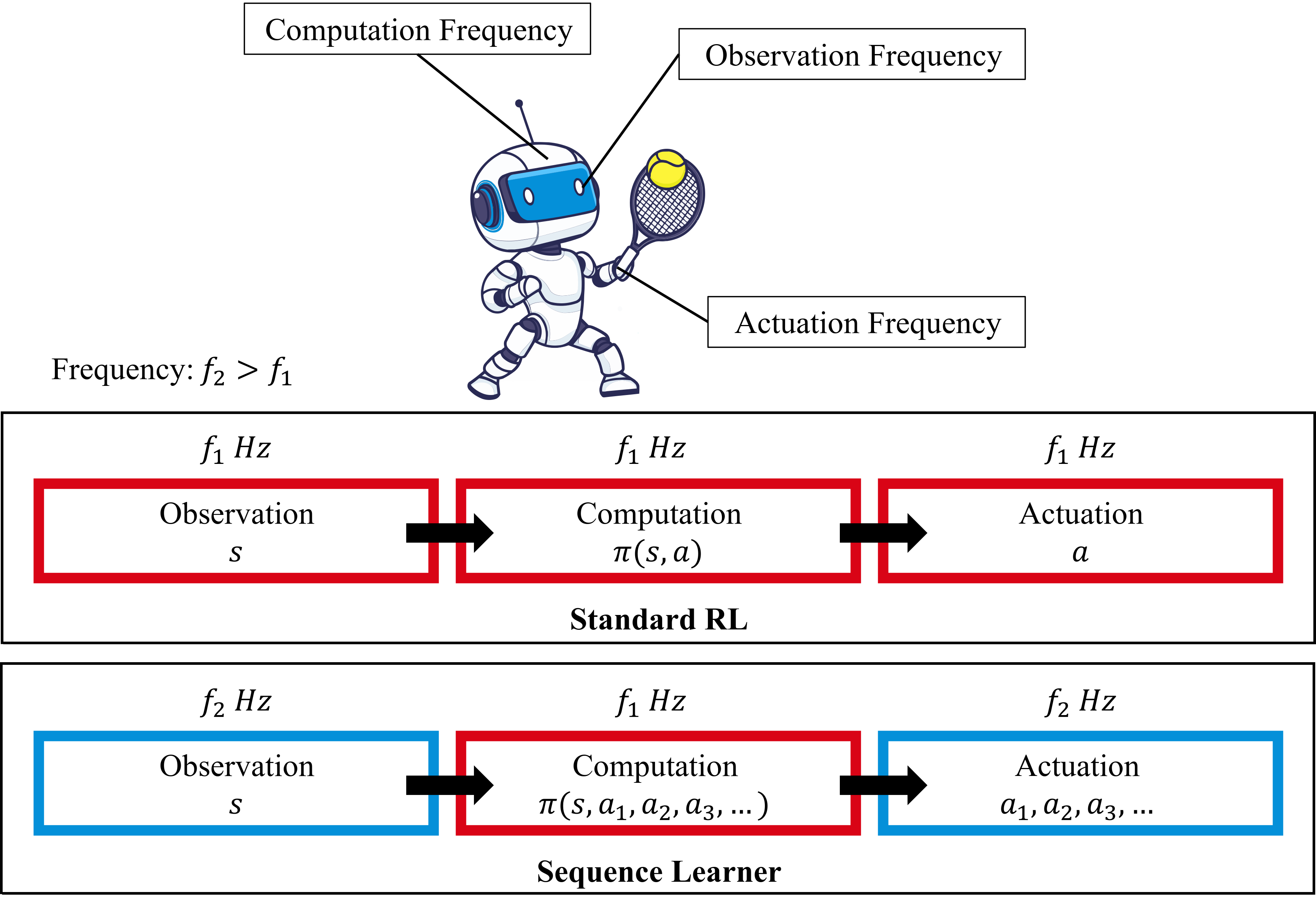
Figure 9: Illustration of the control process in an RL agent, comprising three key components: observation, computation, and actuation. In a standard RL framework, these components typically operate at the same frequency, with each observation leading to a single action after a computation pass. However, the sequence learner can achieve faster actuation by generating multiple primitive actions per observation. It’s important to note that during training, the observation frequency must be at least equal to the actuation frequency and, after training, must match the computation frequency.

To perform any control task, the agent requires the following three components: Sensor, Processor/Computer, Actuator. In the traditional RL framework, all three components act at the same frequency due to the common timestep. However, this is not the case in biological agents that have different sensors of varying frequencies that are often faster than the compute frequency or the speed at which the brain can process the information (Borghuis et al., 2019). Additionally, in order to afford fast and precise control, the actuator frequency is also much faster than the compute frequency (see Figure 9 in Appendix).

It is difficult to exactly measure the speed of computation of the brain. However, one clue lies in the reaction time of humans. The reaction time is the sum of the amount of compute time and the signal transmission delay from the sensor to the processor and the processor to the actuator. It should be noted that delay and the speed/frequency of compute are independent of each other and require different solutions. For example, the brain uses predictive behavior instead of a reactive behavior. However, even with predictive behavior, it is imperative that brain has the ability to actuate at high-frequency with a neurons. This requires a different solution: muscle memory or action chunking described in Section 6. In artificial agents, implementing a similar solution will allow RL algorithms to be deployed into edge devices and cheaper and slower hardware with minimal impact on performance. Delay has been the focus of many previous works (Chen et al., 2020, 2021; Derman et al., 2021), however, adapting to low frequency compute remains an open problem.

3 Related Work

3.1 Model-Based Reinforcement Learning

Model-Based Reinforcement Learning (MBRL) algorithms leverage a model of the environment, which can be either learned or known, to enhance RL performance (Moerland et al., 2023). Broadly, MBRL algorithms have been utilized to:

1. Improve Data Efficiency: By augmenting real-world data with model-generated data, MBRL can significantly enhance data efficiency (Yarats et al., 2021; Janner et al., 2019; Wang et al., 2021).

2. Enhance Exploration: MBRL aids in exploration by using models to identify potential or unexplored states (Pathak et al., 2017; Stadie et al., 2015; Savinov et al., 2018).

3. Boost Performance: Better learned representations from MBRL can lead to improved asymptotic performance (Silver et al., 2017; Levine and Koltun, 2013).

4. Transfer Learning: MBRL supports transfer learning, enabling knowledge transfer across different tasks or environments (Zhang et al., 2018; Sasso et al., 2022).

5. Online Planning: Models can be used for online planning with a single-step policy (Fickinger et al., 2021). However, this approach increases model complexity as each online planning step requires an additional call to the model, making it nonviable for energy and computationally constrained agents like the brain and robots.

Compared to online planning, our algorithm maintains a model complexity of zero after training, eliminating the need for any model calls post-training. This significantly reduces the computational and energy requirements, making it more suitable for practical applications in constrained environments. Additionally, model-based online planning is less biologically plausible than SRL. Wiestler and Diedrichsen (2013) demonstrated that the activations in the motor cortex reduce after skill learning, suggesting that the brain gets more efficient at performing the task after learning. In contrast, model-based online planning does not reduce in the compute and model complexity, but rather might increase in complexity as we perform longer sequences. SRL, on the other hand, has a model complexity of zero after training and thus is biologically plausible based on this observed phenomenon.

3.2 Model Predictive Control

Similar to model-based reinforcement learning, Model Predictive Control (MPC) utilizes a model of the system to predict and optimize future behavior. In the context of modern robotics, MPC has been effectively applied to trajectory planning and real-time control for both ground and aerial vehicles. MPC has been applied to problems like autonomous driving (Gray et al., 2013) and bipedal control (Galliker et al., 2022). However, MPC requires an accurate dynamics model of the system. This limits its practicality to systems that have already been sufficiently modeled. In contrast, SRL does not start with any knowledge of the environment.

Additionally, similar to current RL, MPC requires very fast operational timesteps for practical application. For example, Galliker et al. (2022) implemented walker at 10 ms, Farshidian et al. (2017) implemented a four legged robot at 4 ms and Di Carlo et al. (2018) implemented the MIT Cheetah 3 at 33.33 ms.

3.3 Macro-Actions

Reinforcement Learning (RL) algorithms that utilize macro-actions demonstrate many benefits, including improved exploration and faster learning (McGovern et al., 1997). However, identifying effective macro-actions is a challenging problem due to the curse of dimensionality, which arises from large action spaces. To address this issue, some approaches have employed genetic algorithms (Chang et al., 2022) or relied on expert demonstrations to extract macro-actions (Kim et al., 2020). However, these methods are not scalable and lack biological plausibility.

In contrast, our approach learns macro-actions using the principles of RL, thus requiring little overhead while combining the flexibility of primitive actions with the efficiency of macro-actions.

3.4 Action Repetition and Frame-skipping

To overcome the curse of dimensionality while gaining the benefits of macro-actions, many approaches utilize frame-skipping and action repetition, where macro-actions are restricted to a single primitive action that is repeated. Frame-skipping and action repetition serve as a form of partial open-loop control, where the agent selects a sequence of actions to be executed without considering the intermediate states. Consequently, the number of actions is linear in the number of time steps (Kalyanakrishnan et al., 2021; Srinivas et al., 2017; Biedenkapp et al., 2021; Sharma et al., 2017; Yu et al., 2021).

For instance, FiGaR (Sharma et al., 2017) shifts the problem of macro-action learning to predicting the number of steps that the outputted action can be repeated. TempoRL (Biedenkapp et al., 2021) improved upon FiGaR by conditioning the number of repetitions on the selected actions. However, none of these algorithms can scale to continuous control tasks with multiple action dimensions, as action repetition forces all actuators and joints to be synchronized in their repetitions, leading to poor performance for longer action sequences.

4 Sequence Reinforcement Learning

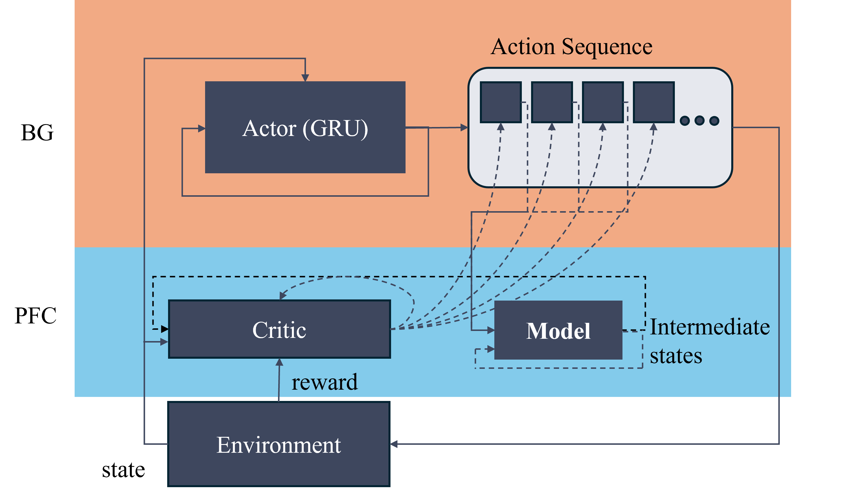
Figure 1: The Sequence Reinforcement Learning (SRL) model. The SRL takes inspiration from the function of the basal ganglia (BG) (Top/Orange) and the prefrontal cortex (PFC) (Bottom/Blue). We train an actor with a gated recurrent unit that can produce sequences of arbitrary lengths given a single state. This is achieved by utilizing a critic and a model that acts at a finer temporal resolution during training/replay to provide an error signal to each primitive action of the action sequence.

Based on the insights presented in Section 6, we introduce a novel reinforcement learning model capable of learning sequences of actions (macro-actions) by replaying memories at a finer temporal resolution than the action generation, utilizing a model of the environment during training.

Components

The Sequence Reinforcement Learning (SRL) algorithm learns to plan ”in-the-mind” using a model during training, allowing the learned action-sequences to be executed without the need for model-based online planning. This is achieved using an actor-critic setting where the actor and critic operate at different frequencies, representing the observation/computation and actuation frequencies, respectively. Essentially, the critic is only used during training/replay and can operate at any temporal resolution, while the actor is constrained to the temporal resolution of the slowest component in the sensing-compute-actuation loop. Denoting the actor’s timestep as $t^{\prime}$ and the critic’s timestep as $t$, our algorithm includes three components:

$$\begin{split}\text{Model }&:s_{t+1}=\textbf{m}_{\phi}(s_{t},a_{t})\\ \text{Critic }&:q_{t}=\textbf{q}_{\psi}(s_{t},a_{t})\\ \text{Actor }&:a_{t^{\prime}}=a_{t^{\prime}},a_{t^{\prime}+t},a_{t^{\prime}+2t}..\sim\pi_{\omega}(s_{t^{\prime}})\end{split}$$ (1)

We denote individual actions in the action sequence generated by actor using the notation $\pi_{\omega}(s_{t^{\prime}})_{t}$ to represent the action $a_{t^{\prime}+t}$

1. Model: Learns the dynamics of the environment, predicting the next state $s_{t+1}$ given the current state $s_{t}$ and primitive action $a_{t}$.

2. Critic: Takes the same input as the model but predicts the Q-value of the state-action pair.

3. Actor: Produces a sequence of actions given an observation at time $t^{\prime}$. Observations from the environment can occur at any timestep $t$ or $t^{\prime}$, where we assume $t^{\prime}>t$. Specifically, in our algorithm, $t^{\prime}=Jt$ where $J>1;J\in\mathbb{Z}$.

Each component of our algorithm is trained in parallel, demonstrating competitive learning speeds.

We follow the Soft-Actor-Critic (SAC) algorithm (Haarnoja et al., 2018) for learning the actor-critic. Exploration and uncertainty are critical factors heavily influenced by timestep size and planning horizon. Many model-free algorithms like DDPG (Lillicrap et al., 2015) and TD3 (Fujimoto et al., 2018) explore by adding random noise to each action during training. However, planning a sequence of actions over a longer timestep can result in additive noise, leading to poor performance during training and exploration. The SAC algorithm addresses this by maximizing the entropy of each action in addition to the expected return, allowing our algorithm to automatically lower entropy for deeper actions farther from the observation.

Learning the Model

The model is trained to minimize the Mean Squared Error of the predicted states. For a trajectory $\tau=(s_{t},a_{t},s_{t+1})$ drawn from the replay buffer $\mathcal{D}$, the predicted state is taken from $\tilde{s}_{t+1}\sim\textbf{m}\phi(s_{t},a_{t})$. The loss function is:

$$\mathcal{L}_{\phi}=\mathbb{E}_{\tau\sim\mathcal{D}}(\tilde{s}_{t+1}-s_{t+1})^{2}$$ (2)

For this work, the model is a feed-forward neural network with two hidden layers. In addition to the current model $\textbf{m}_{\phi}$, we also maintain a target model $\textbf{m}_{\phi^{-}}$ that is the exponential moving average of the current model.

Learning Critic

The critic is trained to predict the Q-value of a given state-action pair $\tilde{q}_{t}=\textbf{q}_{\psi}(s_{t},a_{t})$ using the target value from the modified Bellman equation:

$$\hat{q}_{t}=r_{t}+\gamma\mathbb{E}_{a_{t+1}\sim\pi_{\omega}(s_{t+1})_{0}}[\textbf{q}_{\psi^{-}}(s_{t+1},a_{t+1})-\alpha\log\pi_{\omega}(a_{t+1}|s_{t+1})]$$ (3)

Here, $\textbf{q}_{\psi^{-}}$ is the target critic, which is the exponential moving average of the critic. Following the SAC algorithm, we train two critics and use the minimum of the two $\textbf{q}_{\psi^{-}}$ values to train the current critics. The loss function is:

$$\mathcal{L_{\psi}}=\mathbb{E}_{\tau\sim\mathcal{D}}[(\tilde{q_{t}}_{k}-\hat{q}_{t})^{2}]\forall k\in 1,2$$ (4)

Both critics are feed-forward neural networks with two hidden layers. It should be noted that while the actor utilizes the model during training, the critic does not train on any data generated by the model, thus the critic training is model-free and grounded on the real environment states.

Learning Policy

The SRL policy utilizes two hidden layers followed by a Gated-Recurrent-Unit (GRU) (Cho et al., 2014) that takes as input the previous action in the action sequence, followed by two linear layers that output the mean and standard deviation of the Gaussian distribution of the action. This design allows the policy to produce action sequences of arbitrary length given a single state and the last action.

A naive approach to training a sequence of actions would be to augment the action space to include all possible actions of the sequence length. However, this quickly leads to the curse of dimensionality, as each sequence is considered a unique action, dramatically increasing the policy’s complexity. Additionally, such an approach ignores the temporal information of the action sequence and faces the difficult problem of credit assignment, with only a single scalar reward for the entire action sequence.

To address these problems, we use different temporal scales for the actor and critic. The critic assigns value to each primitive action of the action sequence, bypassing the credit assignment problem caused by the single scalar reward. However, using collected state-action transitions to train the action sequence is impractical, as changing the first action in the sequence would render all future states inaccurate. Thus, the model populates intermediate states, which the critic then uses to assign value to each primitive action in the sequence.

Therefore, given a trajectory $\tau=(a_{t-1},s_{t},a_{t},s_{t+1})$, we first produce the $J$-step action sequence using the policy: $\tilde{a}_{t:t+J}\sim\pi_{\omega}(s_{t})$. We then iteratively apply the target model to get the intermediate states $\tilde{s}_{t+1:t+J-1}$. Finally, we use the critic to calculate the loss for the actor as follows:

$$\mathcal{L}_{\omega}=\mathbb{E}_{\tau\sim\mathcal{D}}\bigg{[}\alpha\log\pi_{\omega}(\tilde{a}_{t}|s_{t})-\textbf{q}_{\psi}(s_{t},\tilde{a}_{t})+\sum_{j=1}^{J}\alpha\log\pi_{\omega}(\tilde{a}_{t+j}|\tilde{s}_{t+j})-\textbf{q}_{\psi}(\tilde{s}_{t+j},\tilde{a}_{t+j})\bigg{]}$$ (5)

5 Experiments

Overview

We evaluate our SRL approach on several continuous control tasks, comparing it against the SAC baseline. Our focus is on environments with multi-dimensional actions, ranging from the simple LunarLanderContinuous (2 action dimensions) to the complex Humanoid environment (17 action dimensions). This allows us to highlight the benefits of SRL over traditional action repetition approaches. We utilize the OpenAI gym (Brockman et al., 2016) implementation of the MuJoCo environments (Todorov et al., 2012).

Experiemental Setup

We train SRL with four different action sequence lengths (ASL), $J={2,4,8,16}$, referred to as SRL-$J$. During training, SRL is evaluated based on its $J$ value, processing states only after every $J$ actions. All hyperparameters are identical between SRL and SAC, except for the actor update frequency: SRL updates the actor every 4 steps, while SAC updates every step. Thus, SAC has four more actor update steps compared to SRL. Additionally, SRL learns a model in parallel with the actor and critic.

We presents the learning curves of SRL and SAC across 10 continuous control tasks in the appendix. We observe that SRL outperforms SAC in six out of ten tasks. Notably, SRL-16 achieves competitive performance on LunarLander, Hopper, Reacher and Swimmer tasks, showcasing the algorithm’s capability to learn long action sequences from scratch. Surprisingly, SRL also outperforms SAC in the Humanoid environment with fewer inputs and actor updates while concurrently learning a model, demonstrating the efficacy of the algorithm on environments with higher action dimensions. It should be noted that the learning curves presented for SRL-$J$ take in states every $J$ steps, thus SRL is evaluated on a disadvantage in the learning curves.

Frequency-Averaged Score

Figure 2: Performance of SRL and SAC at different Action Sequence Lengths (ASL) for the Hopper environment. All markers are averaged over 5 trials, with the error bars representing standard error. The Frequency-Averaged Score (FAS) is calculated as the area under the curve of this plot.

Transitioning from simulation to real-world implementation (Sim2Real) in control systems is challenging because deployment introduces computational stochasticity, leading to variable sensor sampling rates and inconsistent end-to-end delays from sensing to actuation (Sandha et al., 2021). This gap is not captured by the mean reward or return that is the norm in current RL literature. To address this, we introduce Frequency-Averaged Score (FAS) that is the normalized area under the curve (AUC) of the performance vs. decision frequency plot. Figure 2 demonstrates the plot over which FAS is calculated for the Hopper environment. We provide similar plots for all environments in the Appendix. The FAS captures the overall performance of the policy at different decision frequencies, timesteps or macro-action lengths. A High FAS indicates that the policy performance generalizes across:

1. Decision frequencies

2. Observation frequencies

3. Timestep sizes

The Frequency Averaged Score (FAS) is developed to assess the overall performance of a single policy across multiple frequency settings, rather than evaluating algorithmic efficacy by training and testing separate policies for each individual frequency. A high FAS reflects a policy’s robustness and adaptability, indicating that it can be effectively deployed across varying frequencies without the need for retraining.

Environment	SAC	SRL-2	SRL-4	SRL-8	SRL-16
Lunar Lander	0.20 $\pm$ 0.09	0.12 $\pm$ 0.09	0.52 $\pm$ 0.11	0.63 $\pm$ 0.21	0.89 $\pm$ 0.05
Hopper	0.04 $\pm$ 0.02	0.09 $\pm$ 0.02	0.21 $\pm$ 0.04	0.36 $\pm$ 0.06	0.44 $\pm$ 0.04
Walker2d	0.07 $\pm$ 0.01	0.11 $\pm$ 0.02	0.24 $\pm$ 0.05	0.26 $\pm$ 0.06	0.21 $\pm$ 0.10
Ant	-0.05 $\pm$ 0.04	0.05 $\pm$ 0.01	0.26 $\pm$ 0.09	0.38 $\pm$ 0.14	0.47 $\pm$ 0.11
HalfCheetah	0.01 $\pm$ 0.01	0.05 $\pm$ 0.01	0.12 $\pm$ 0.02	0.20 $\pm$ 0.01	0.25 $\pm$ 0.01
Humanoid	0.06 $\pm$ 0.01	0.07 $\pm$ 0.00	0.17 $\pm$ 0.02	0.27 $\pm$ 0.04	0.38 $\pm$ 0.05
InvPendulum	0.05 $\pm$ 0.02	0.08 $\pm$ 0.01	0.16 $\pm$ 0.04	0.18 $\pm$ 0.04	0.23 $\pm$ 0.06
InvDPendulum	0.02 $\pm$ 0.00	0.04 $\pm$ 0.01	0.05 $\pm$ 0.02	0.02 $\pm$ 0.02	0.02 $\pm$ 0.00
Reacher	0.65 $\pm$ 0.07	0.87 $\pm$ 0.01	0.89 $\pm$ 0.00	0.91 $\pm$ 0.00	0.92 $\pm$ 0.00
Swimmer	0.19 $\pm$ 0.05	0.32 $\pm$ 0.05	0.37 $\pm$ 0.18	0.31 $\pm$ 0.03	0.39 $\pm$ 0.16

Table 2: Mean Frequency-Averaged Score (FAS) and standard deviation for different environments with SAC and various SRL configurations (rounded to two decimals, highest value highlighted). Each value is averaged over 5 trials. We see that SRL provides a significant improvement over SAC.

Table 2 presents the Frequency Averaged Score (FAS) metric for SAC and SRL across varying action lengths. In most environments, SRL-16 demonstrates strong and consistent performance across a broad range of frequencies. However, in the Walker2d-v2 and InvertedDoublePendulum-v2 environments, SRL struggles with learning longer action sequences. We hypothesize that this challenge arises from higher modeling errors in these environments, and believe that improved environmental models could enhance these results—a direction we leave for future exploration. Notably, SAC performed poorly across all environments, underscoring the limitations of traditional RL methods in adapting to frequency changes and reinforcing the importance of our approach.

In order to further validate the utility of FAS, we test all the policies (SAC and SRL) in a stochastic timestep environment. The timestep (time until next input) is randomly chosen from a uniform distribution of integers in [1,16] after each decision. This is a more realistic setting as it tests the performance of the policy in when the frequency is not constant. Each policy is evaluated over 10 episodes with stochastic timesteps.

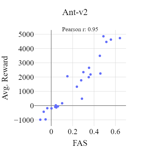
Figure 3: Avg. Reward vs FAS of different policies on stochastic timestep evaluations. Each marker is averaged over 10 episodes.

Figure 3 plots the performance of each policy vs. its individual FAS. As shown, FAS and the performance on a stochastic timestep environment has a high Pearson correlation ratio of 0.95, thus validating the utility of FAS as a metric to measure generalized performance of a policy across timesteps and frequencies. We provide similar plots for all environments in the appendix.

Comparison to Model-based Online Planning

In addition to action repetition, model-based online planning is another approach that allows the RL agent to reduce its observational frequency. However, it often requires a highly accurate model of the environment and incurs increased model complexity due to the use of the model during control. Despite these challenges, comparing SRL to model-based online planning is essential since it is useful when the actor cannot produce long sequences of actions and does not require the hyper-parameter $J$. With access to an accurate model of the environment, the agent’s performance might generalize to arbitrary ASL.

Since SRL incorporates a model of the environment that is learned in parallel, we compare the performance of the SRL actor utilizing the actor-generated action sequences against model-based online planning, where the actor produces only a single action between each simulated state.

Environment	SRL	Online Planning	State Space	Action Space
Lunar Lander	0.89 $\pm$ 0.05	0.79 $\pm$ 0.08	8	2
Hopper	0.44 $\pm$ 0.04	0.59 $\pm$ 0.19	11	3
Walker2d	0.26 $\pm$ 0.06	0.20 $\pm$ 0.05	17	6
Ant	0.47 $\pm$ 0.11	0.34 $\pm$ 0.08	27	8
HalfCheetah	0.25 $\pm$ 0.01	0.19 $\pm$ 0.02	17	6
Humanoid	0.38 $\pm$ 0.05	0.18 $\pm$ 0.03	376	17
InvPendulum	0.23 $\pm$ 0.06	0.63 $\pm$ 0.10	4	1
InvDPendulum	0.04 $\pm$ 0.01	0.10 $\pm$ 0.07	11	1
Reacher	0.92 $\pm$ 0.00	0.95 $\pm$ 0.00	11	2
Swimmer	0.39 $\pm$ 0.16	0.43 $\pm$ 0.14	8	2

Table 3: Comparison of the FAS of SRL and corresponding model-based online planning policies across different environments.

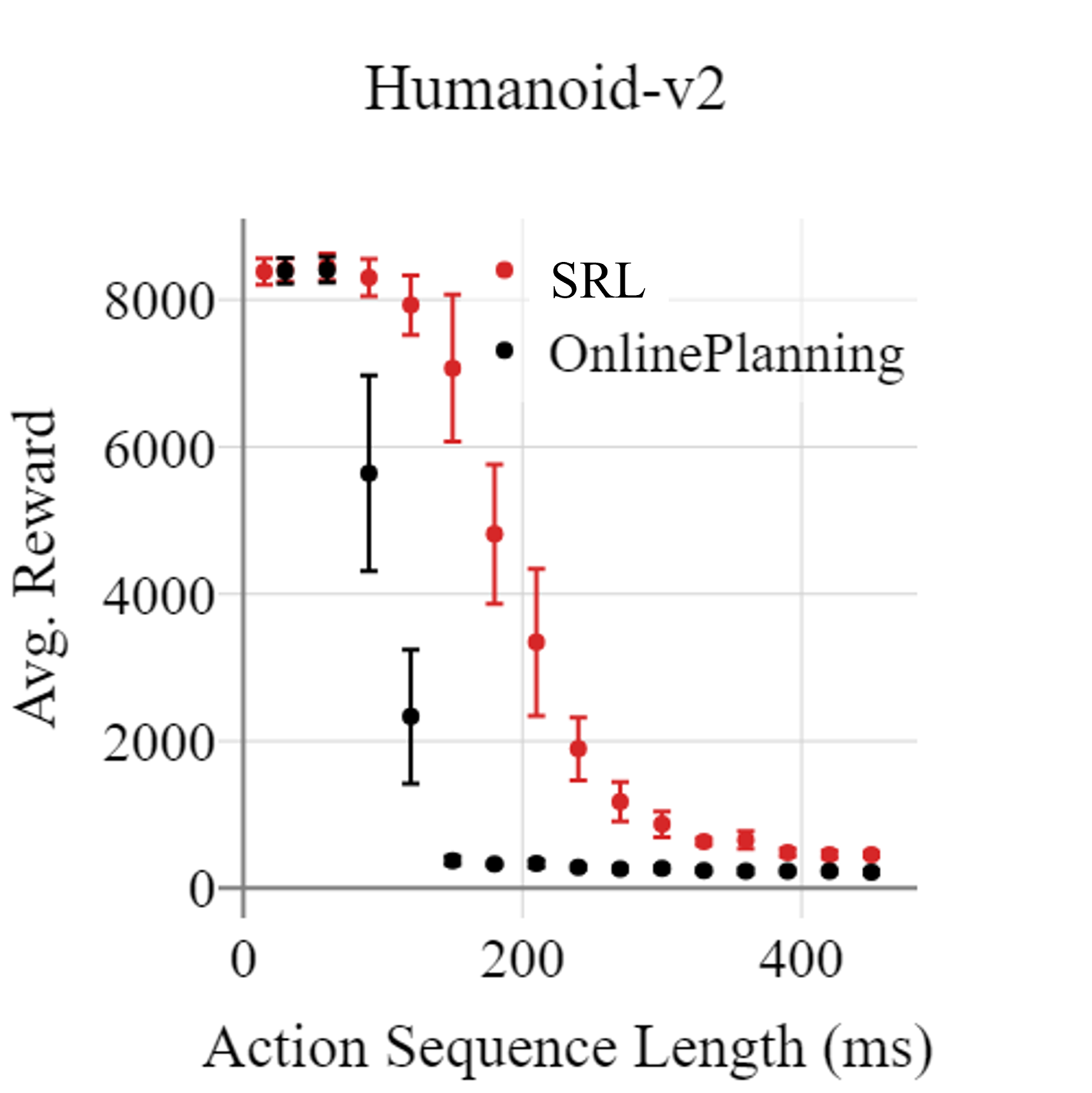
Figure 4: Performance of SRL and model based online planning on different ASL. All markers are averaged over 5 trials. The error bars show standard error.

Table 3 compares the FAS score SRL to online planning using the same model in online planning versus the action sequences generated by the SRL policy. We see that SRL can learn action sequences that perform better than model-based online planning in many environments. Notably, SRL performs better in environments with larger action and state space dimensions (See Figure 4 for example of Humanoid). Such environments are harder to model. Thus, SRL can leverage inaccurate models to learn accurate action sequences, further reducing the required computational complexity during training. We hypothesize that this superior performance is due to the fact that the actor learns a $J$-step action sequence concurrently, while online planning only produces one action at a time. Consequently, SRL is able to learn and produce long, coherent action sequences, whereas single-step predictions tend to drift, similar to the ”hallucination” phenomenon observed in transformer-based language models.

6 Neural Basis for Sequence Learning

Unlike artificial RL agents, learning in the brain does not stop once an optimal solution has been found. During initial task learning, brain activity increases as expected, reflecting neural recruitment. However, after training and repetition, activity decreases as the brain develops more efficient representations of the action sequence, commonly referred to as muscle memory (Wiestler and Diedrichsen, 2013). This phenomenon is further supported by findings that sequence-specific activity in motor regions evolves based on the amount of training, demonstrating skill-specific efficiency and specialization over time (Wymbs and Grafton, 2015).

The neural basis for action sequence learning involves a sophisticated interconnection of different brain regions, each making a distinct contribution:

1. Basal ganglia (BG): Action chunking is a cognitive process by which individual actions are grouped into larger, more manageable units or ”chunks,” facilitating more efficient storage, retrieval, and execution with reduced cognitive load (Favila et al., 2024). Importantly, this mechanism allows the brain to perform extremely fast and precise sequences of actions that would be impossible if produced individually. The BG plays a crucial role in chunking, encoding entire behavioral action sequences as a single action (Jin et al., 2014; Favila et al., 2024; Jin and Costa, 2015; Berns and Sejnowski, 1996, 1998; Garr, 2019). Dysfunction in the BG is associated with deficits in action sequences and chunking in both animals (Doupe et al., 2005; Jin and Costa, 2010; Matamales et al., 2017) and humans (Phillips et al., 1995; Boyd et al., 2009; Favila et al., 2024). However, the neural basis for the compression of individual actions into sequences remains poorly understood.

2. Prefrontal cortex (PFC): The PFC is critical for the active unbinding and dismantling of action sequences to ensure behavioral flexibility and adaptability (Geissler et al., 2021). This suggests that action sequences are not merely learned through repetition; the PFC modifies these sequences based on context and task requirements. Recent research indicates that the PFC supports memory elaboration (Immink et al., 2021) and maintains temporal context information (Shahnazian et al., 2022) in action sequences. The prefrontal cortex receives inputs from the hippocampus.

3. Hippocampus (HC) replays neuronal activations of tasks during subsequent sleep at speeds six to seven times faster. This memory replay may explain the compression of slow actions into fast chunks. The replayed trajectories from the HC are consolidated into long-term cortical memories (Zielinski et al., 2020; Malerba et al., 2018). This phenomenon extends to the motor cortex, which replays motor patterns at accelerated speeds during sleep (Rubin et al., 2022).

7 Discussion, Limitations and Future Work

We introduce the Sequence Reinforcement Learning (SRL) algorithm, a biologically plausible model for sequence learning. It represents a significant step towards achieving robust control at brain-like speeds. The key contributions of SRL include its ability to generate long sequences of actions from a single state, its resilience to reduced input frequency, and its lower computational complexity per primitive action.

The current RL framework encourages synchrony between the environment and the components of the agent. However, the brain utilizes components that act at different frequencies and yet is capable of robust and accurate control. SRL provides an approach to reconcile this difference between neuroscience and RL, while remaining competitive on current RL benchmarks. SRL offers substantial benefits over traditional RL algorithms, particularly in the context of autonomous agents such as self-driving cars and robots. By enabling operation at slower observational frequencies and providing a gradual decay in performance with reduced input frequency, SRL addresses critical issues related to sensor failure and occlusion, and energy consumption. Additionally, SRL generates long sequences of actions from a single state, which can enhance the explainability of the policy and provide opportunities to override the policy early in case of safety concerns. SRL also learns a latent representation of the action sequence, which could be used in the future to interface with large language models for multimodal explainability and even hierarchical reinforcement learning and transfer learning.

Future Work

We believe the SRL model contributes to both artificial agents and the study of biological control. Future work will incorporate biological features like attention mechanisms and knowledge transfer. Additionally, SRL can benefit from existing Model-Based RL approaches as it naturally learns a model of the world. In the Appendix, we demonstrate preliminary results of generative replay in the latent space. We believe that this is a promising direction to significantly improve upon the results in the paper.

In deterministic environments, a capable agent should achieve infinite horizon control for tasks like walking and hopping from a single state. This is an important research direction that is currently underexplored, as many environments are partially observable or have some degree of stochasticity. Current approaches rely on external information at every state, which increases energy consumption and vulnerability to adversarial or missing inputs. Truly autonomous agents will need to implement multiple policies simultaneously, and simple tasks like walking can be performed without input states if learned properly. Our future work will focus on extending the action sequence horizon until deterministic tasks can be performed using a single state and implementing a mechanism to dynamically pick the action sequence horizon based on context and predictability of the state. Serotonin is an important neuromodulator that has been demonstrated to signal the availability of time and resources in the brain to enable the decision on the planning horizon and the use of compute (Doya et al., 2021). In the future, we hope to introduce a mechanism to replicate the effect of serotonin in SRL to modulate the sequence length automatically based on context.

8 Conclusion

In this paper, we introduced Sequence Reinforcement Learning (SRL): a model based action sequence learning algorithm for model free control. We demonstrated the improvement of SRL over existing framework by testing it over various control frequencies. Furthermore, we introduces the Frequency-Averaged-Score (FAS) metric to measure the robustness of a policy across different frequencies. Our work is the first to achieve competitive results on continuous control environments at low control frequencies and serves as a benchmark for future work in this direction. Finally, we demonstrated directions for future works including comparison to model-based planning, generative replay and connections to neuroscience.

Appendix A Appendix

A.1 SRL Algorithm

Input: $\phi,\psi_{1},\psi_{2},\omega$. Initial parameters

$\bar{\phi}\leftarrow\phi,\bar{\psi}_{1}\leftarrow\psi_{1}$, $\bar{\psi}_{2}\leftarrow\psi_{2}$ ;

  // Initialize target network weights

$D\leftarrow\emptyset$ ;

  // Initialize an empty replay pool

1 for each iteration do

       $\{a_{t},a_{t+1},\ldots,a_{t+J-1}\}\sim\pi_{\omega}(\{a_{t},a_{t+1},\ldots,a_{t+J-1}\}|s_{t})$ ;

        // Sample action sequence from the policy

2      

3      for each action $a_{t}$ in the sequence do

             $s_{t+1}\sim p(s_{t+1}|s_{t},a_{t})$ ;

              // Sample transition from the environment

             $D\leftarrow D\cup\{(s_{t},a_{t},r(s_{t},a_{t}),s_{t+1})\}$ ;

              // Store transition in the replay pool

4            

5       end for

6      for each gradient step do

             $\phi\leftarrow\phi-\lambda_{\textbf{m}}\nabla_{\phi}\mathcal{L}_{\phi}$ ;

              // Update the model parameters

7            

8            for $i\in\{1,2\}$ do

                   $\psi_{i}\leftarrow\psi_{i}-\lambda_{Q}\nabla_{\psi_{i}}\mathcal{L}_{\psi_{i}}$ ;

                    // Update the Q-function parameters

9                  

10             end for

            $\{a_{t},a_{t+1},\ldots,a_{t+J-1}\}\sim\pi_{\omega}(\{a_{t},a_{t+1},\ldots,a_{t+J-1}\}|s_{t})$ ;

              // Sample action sequence from the policy

11            

12            if iteration mod actor_update_frequency == 0 then

13                   for $j\in\{1,\ldots,J\}$ do

14                        

                        $s_{j+1}\sim\textbf{m}_{\bar{\phi}}(s_{j+1}|s_{j},a_{j})$ ;

                          // Sample transition from the target model

15                        

16                   end for

                  $\phi\leftarrow\omega-\lambda_{\pi}\nabla_{\omega}L_{\omega}$ ;

                    // Update policy weights

17                  

18             end if

19            

            $\alpha\leftarrow\alpha-\lambda\nabla_{\hat{\alpha}}\mathcal{L}(\alpha)$ ;

              // Adjust temperature

20             for $i\in\{1,2\}$ do

                   $\bar{\psi}_{i}\leftarrow\tau\psi_{i}+(1-\tau)\bar{\psi}_{i}$ ;

                    // Update target network weights

21                  

22             end for

            $\bar{\phi}\leftarrow\tau\phi+(1-\tau)\bar{\phi}$ ;

              // Update target model weights

23            

24       end for

25      

26 end for

Output: $\phi,\psi_{1},\psi_{2},\omega$;

  // Optimized parameters

27

Algorithm 1 Sequence Reinforcement Learning

Hyperparameters

The table below lists the hyperparameters that are common between every environment used for all our experiments for the SAC and SRL algorithms:

Hyperparameter	Value	description
Hidden Layer Size	256	Size of the hidden layers in the feed forward networks of Actor, Critic, Model and Encoder networks
Updates per step	1	Number of learning updates per one step in the environment
Target Update Interval	1	Inverval between each target update
$\gamma$	0.99	Discount Factor
$\tau$	0.005	Update rate for the target networks (Critic and Model)
Learning Rate	0.0003	Learning rate for all neural networks
Replay Buffer Size	$10^{6}$	Size of the replay buffer
Batch Size	256	Batch size for learning
Start Time-steps	10000	Initial number of steps where random policy is followed

Table 4: List of Common hyperparameters

Environment	max Timestep	Eval frequency
LunarLanderContinuous-v2	500000	2500
Hopper-v2	1000000	5000
Walker2d-v2	1000000	5000
Ant-v2	5000000	5000
HalfCheetah-v2	5000000	5000
Humanoid-v2	10000000	5000

Table 5: List of environment-specific hyperparameters

A.2 Implementation Details

Due to its added complexity during training, SRL requires longer wall clock time for training when compared to SAC. We performed a minimal hyperparameter search over the actor update frequency parameter on the Hopper environment (tested values: 1, 2, 4, 8, 16). All the other hyperparamters were picked to be equal to the SAC implementation. We also did not perform a hyerparameter search over the size of GRU for the actor. It was picked to have the same size as the hidden layers of the feed forward network of the actor in SAC. The neural network for the model was also picked to have the same architecture as the actor from SAC, thus it has two hidden layers with 256 neurons. Similarly the encoder for the latent SRL implementation was also picked to have the same architecture. For the latent SRL implementation we also add an additional replay buffer to store transitions of length 5, to implement the temporal consistency training for the model. This was done for simplicity of the implementation, and it can be removed since it is redundant to save memory.

All experiments were performed on a GPU cluster the Nvidia 1080ti GPUs. Each run was performed using a single GPU, utilizing 8 CPU cores of Intel(R) Xeon(R) Silver 4116 (24 core) and 16GB of memory.

We utilize the pytorch implementation of SAC (https://github.com/denisyarats/pytorch_sac) [Yarats and Kostrikov, 2020].

Learning Curves

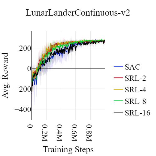
(a)

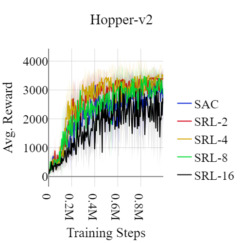
(b)

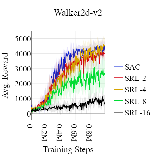
(c)

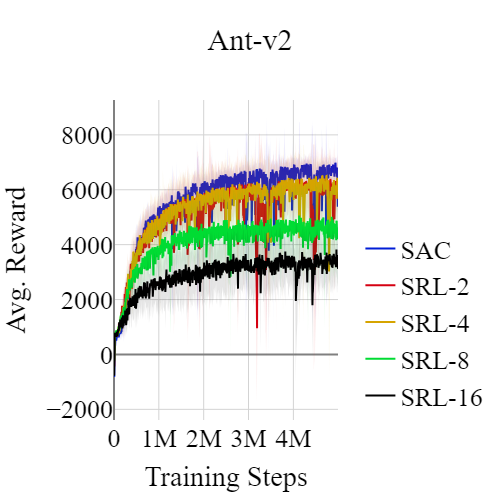
(d)

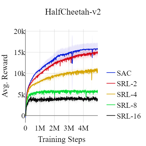
(e)

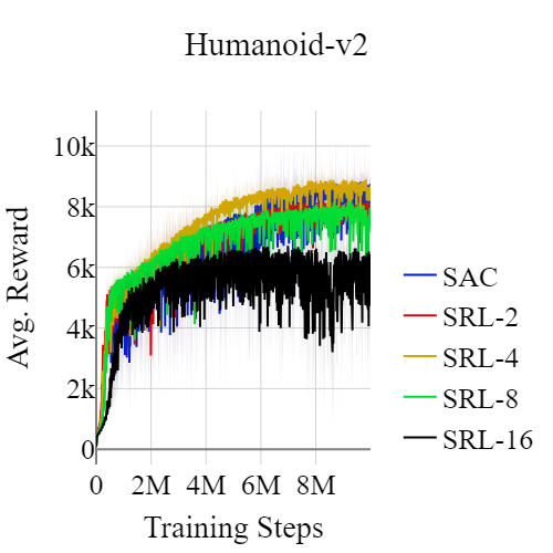
(f)

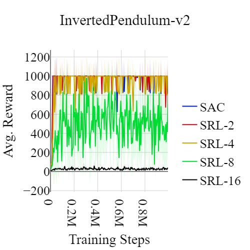
(g)

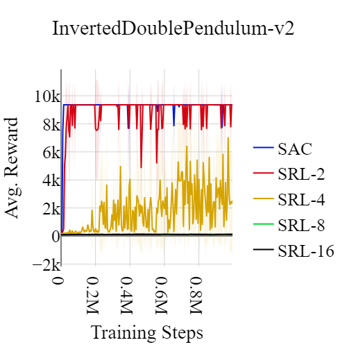
(h)

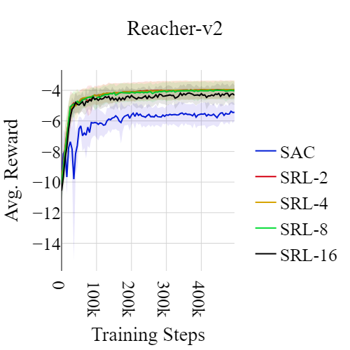
(i)

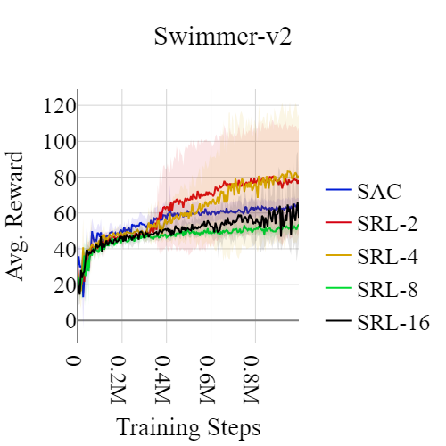
(j)

Figure 5: Learning curves of SRL-$J$ and Soft-Actor Critic (SAC) [Haarnoja et al., 2018] over continuous control tasks. SRL and SAC are evaluated under different settings: SAC receives input after every primitive action, while SRL receives input after $J$ primitive actions. Yet it demonstrates competitive performance on all environments, even outperforming SAC on LunarLander, Hopper, Walker, Humanoid, Reacher and Swimmer environments. SRL demonstrates stable learning even with the added model and generative replay training. All curves are averaged over 5 trials, with shaded regions representing standard deviation.

A.3 Plots for Frequency Averaged Scores

Figure 6 shows the plots for FAS. The ASL of 1 in the figure represents the performance of each policy in the standard reinforcement learning setting. We can see that SRL is competitive with SAC on ASL of 1 on all environments tested. Larger $H$ results in better robustness at longer ASLs but it often comes at the cost of lower performance at shorter ASLs.

Additionally, as the FAS reflects, SRL is also significantly more robust across different frequencies than standard RL (SAC).

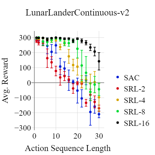
(a)

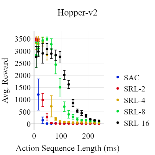
(b)

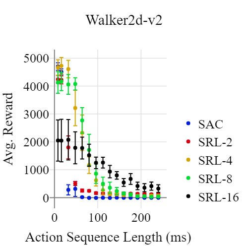
(c)

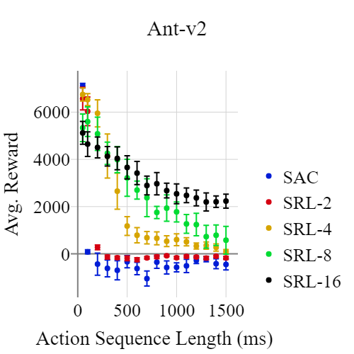
(d)

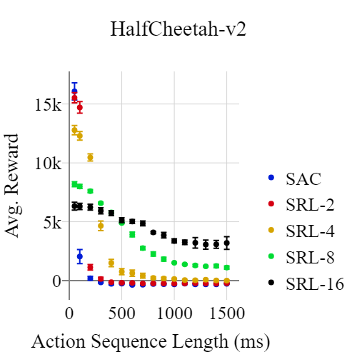
(e)

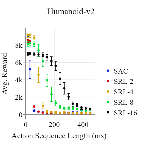
(f)

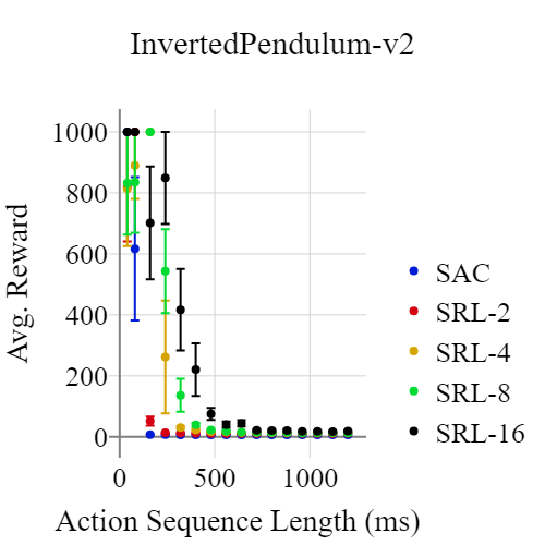
(g)

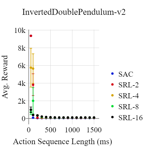
(h)

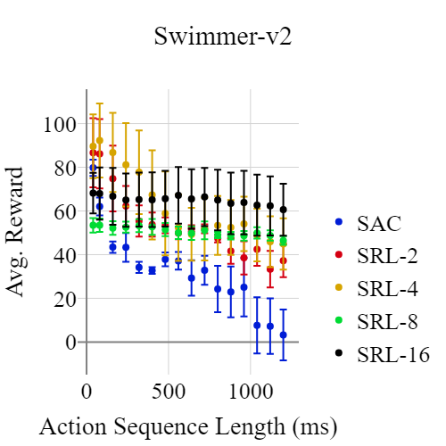
(i)

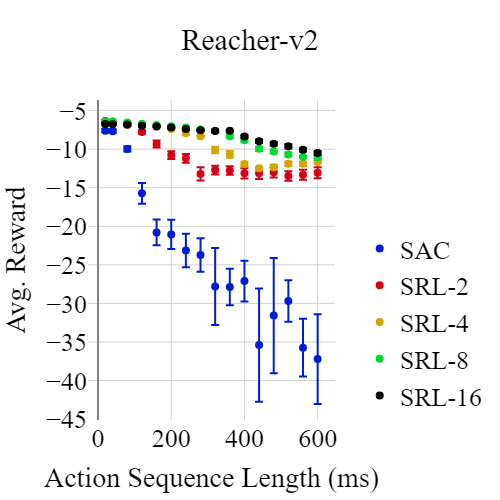
(j)

Figure 6: Performance of SRL and SAC at different Action Sequence Lengths (ASL). SAC repeats the same action for the duration, while SRL can perform a sequence of actions. All policies were tested on ASL of 1, 2, 4, 8 … 30. All markers are averaged over 5 trials, with the error bars representing standard error.

A.4 Plots for FAS vs. Stochastic Timestep Performance

In Figure 7, we present the plots for FAS vs performance for all environments. For all environments except InvertedDoublePendulum-v2, we see a high correlation. InvertedDoublePendulum-v2 is a difficult problem at slow frequency and demonstrates poor performance of less than 200, thus it does not correlate to FAS.

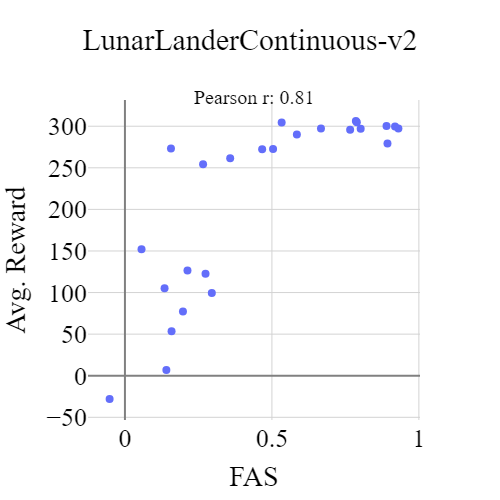
(a)

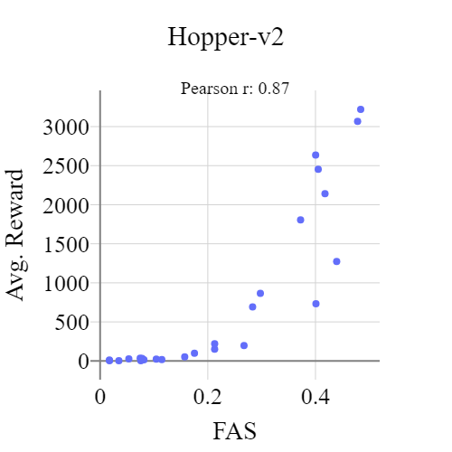
(b)

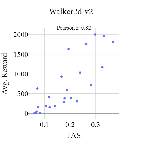
(c)

(d)

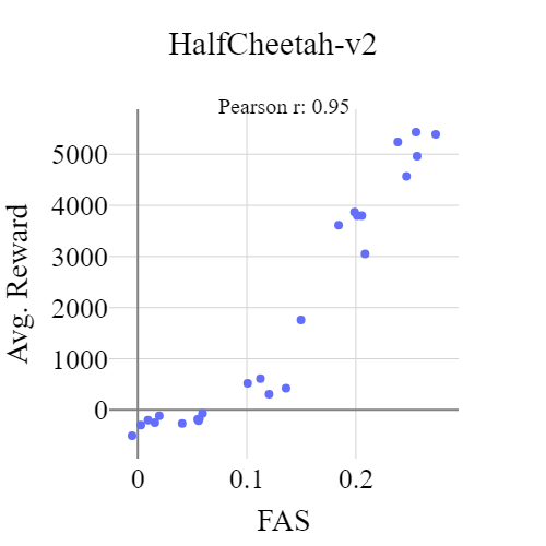
(e)

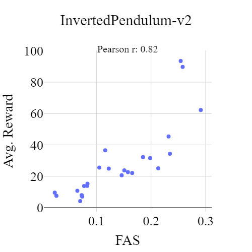
(f)

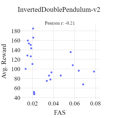
(g)

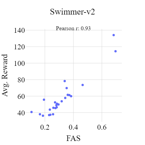
(h)

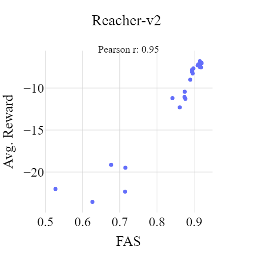
(i)

Figure 7: Performance vs. FAS of different policies (SAC, SRL-2, SRL-4, SRL-8, SRL-16). For each algorithm, we test 5 policies over 10 episodes.

A.5 Generative Replay in Latent Space

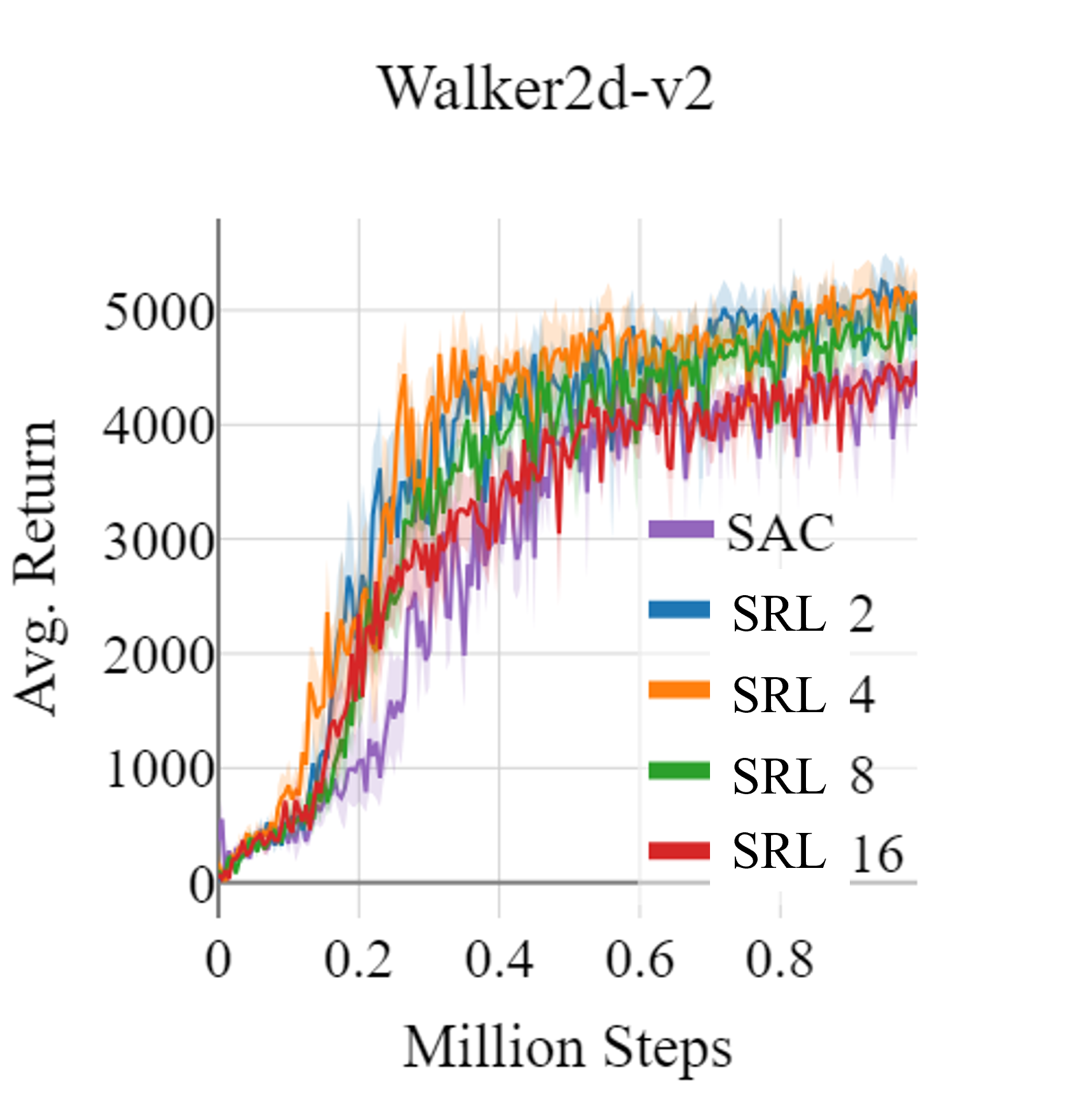
(a)

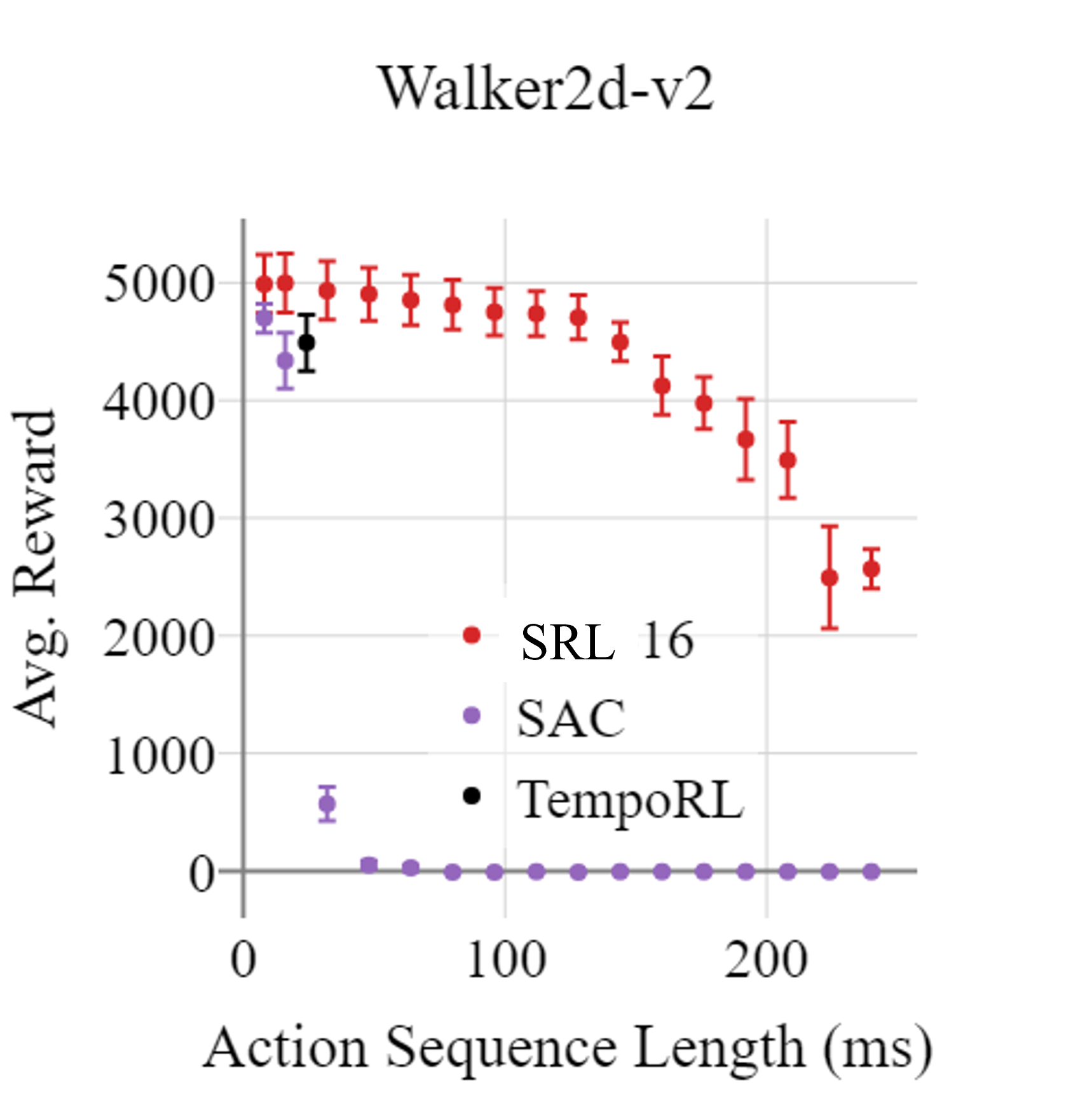
(b)

Figure 8: Left: Learning curve of SRL with latent state-space on the Walker2d-v2 environment. Right: Performance of latent SRL-16 on different ASL, compared to SAC and TempoRL. Utilizing a latent representation for state space is especially beneficial for the Walker2d environment so that it outperforms SAC even when training upto sequence lengths of $J=16$.

Previous studies have shown that generative replay benefits greatly from latent representations [Van de Ven et al., 2020]. Recently, Simplified Temporal Consistency Reinforcement Learning (TCRL) [Zhao et al., 2023] demonstrated that learning a latent state-space improves not only model-based planning but also model-free RL algorithms. Building on this insight, we introduced an encoder to encode the observations in our algorithm.

Following the TCRL implementation, we use two encoders: an online encoder $\textbf{e}_{\theta}$ and a target encoder $\textbf{e}_{\theta^{-}}$, which is the exponential moving average of the online encoder:

$$\begin{split}\text{Encoder}&:e_{t}=\textbf{e}_{\theta}(s_{t})\end{split}$$ (6)

Thus, the model predicts the next state in the latent space. Additionally, we introduce multi-step model prediction for temporal consistency. Following the TCRL work, we use a cosine loss for model prediction. The model itself predicts only a single step forward, but we enforce temporal consistency by rolling out the model $H$-steps forward to predict $\tilde{e}_{t+1:t+1+H}$.

Specifically, for an $H$-step trajectory $\tau=(z_{t},a_{t},z_{t+1})_{t:t+H}$ drawn from the replay buffer $\mathcal{D}$, we use the online encoder to get the first latent state $e_{t}=\textbf{e}_{\theta}(o_{t})$. Then conditioning on the sequence of actions $a_{t:t+H}$, the model is applied iteratively to predict the latent states $\tilde{e}_{t+1}=\textbf{m}_{\phi}(\tilde{e}_{t},a_{t})$. Finally, we use the target encoder to calculate the target latent states $\hat{e}_{t+1:t+H+1}=\textbf{e}_{\theta^{-}}(o_{t+1:t+1+H})$. The Loss function is defined as:

$$\mathcal{L}_{\theta,\phi}=\mathbb{E}_{\tau\sim\mathcal{D}}\bigg{[}\sum_{h=0}^{H}-\gamma^{h}\bigg{(}\frac{\tilde{e}_{t+h}}{||\tilde{e}_{t+h}||_{2}}\bigg{)}^{T}\bigg{(}\frac{\hat{e}_{t+h}}{||\hat{e}_{t+h}||_{2}}\bigg{)}\bigg{]}$$ (7)

We set $H=5$ for our experiments. Both the encoder and the model are feed-forward neural networks with two hidden layers.

We provide preliminary results for the Walker environment. Utilizing the latent space for generative replay significantly improved performance, making it competitive even at 16 steps (128ms) (Figure 8).

We also provide the TempoRL [Biedenkapp et al., 2021] algorithm as a benchmark as it is an algorithm that successfully reduces the number of decisions per episodes. TempoRL is designed to dynamically pick the best frameskip (for performance), therefore we report the avg. action sequence length for TempoRL.

A.6 Clarification Figure

References

- Sutton and Barto [2018] Richard S Sutton and Andrew G Barto. Reinforcement learning: An introduction. MIT press, 2018.
- Schultz et al. [1997] W. Schultz, P. Dayan, and P. R. Montague. A neural substrate of prediction and reward. Science, 275:1593–1599, 1997. ISSN 00368075. doi: 10.1126/SCIENCE.275.5306.1593/ASSET/6CC77AD2-EA4B-4861-A4ED-A076123F94E0/ASSETS/GRAPHIC/SE1174905004.JPEG. URL https://www.science.org/doi/10.1126/science.275.5306.1593.
- Schultz [2015] Wolfram Schultz. Neuronal reward and decision signals: From theories to data. Physiological Reviews, 95:853–951, 7 2015. ISSN 15221210. doi: 10.1152/PHYSREV.00023.2014/ASSET/IMAGES/LARGE/Z9J0031527320049.JPEG. URL https://journals.physiology.org/doi/10.1152/physrev.00023.2014.
- Cohen et al. [2012] Jeremiah Y. Cohen, Sebastian Haesler, Linh Vong, Bradford B. Lowell, and Naoshige Uchida. Neuron-type-specific signals for reward and punishment in the ventral tegmental area. Nature 2012 482:7383, 482:85–88, 1 2012. ISSN 1476-4687. doi: 10.1038/nature10754. URL https://www.nature.com/articles/nature10754.
- OpenAI et al. [2019] OpenAI, Christopher Berner, Greg Brockman, Brooke Chan, Vicki Cheung, Przemysław Debiak, Christy Dennison, David Farhi, Quirin Fischer, Shariq Hashme, Chris Hesse, Rafal Józefowicz, Scott Gray, Catherine Olsson, Jakub Pachocki, Michael Petrov, Henrique P. d. O. Pinto, Jonathan Raiman, Tim Salimans, Jeremy Schlatter, Jonas Schneider, Szymon Sidor, Ilya Sutskever, Jie Tang, Filip Wolski, and Susan Zhang. Dota 2 with large scale deep reinforcement learning. 12 2019. URL https://arxiv.org/abs/1912.06680v1.
- Schrittwieser et al. [2020] Julian Schrittwieser, Ioannis Antonoglou, Thomas Hubert, Karen Simonyan, Laurent Sifre, Simon Schmitt, Arthur Guez, Edward Lockhart, Demis Hassabis, Thore Graepel, Timothy Lillicrap, and David Silver. Mastering atari, go, chess and shogi by planning with a learned model. Nature 2020 588:7839, 588:604–609, 12 2020. ISSN 1476-4687. doi: 10.1038/s41586-020-03051-4. URL https://www.nature.com/articles/s41586-020-03051-4.
- Kaufmann et al. [2023a] Elia Kaufmann, Leonard Bauersfeld, Antonio Loquercio, Matthias Müller, Vladlen Koltun, and Davide Scaramuzza. Champion-level drone racing using deep reinforcement learning. Nature 2023 620:7976, 620:982–987, 8 2023a. ISSN 1476-4687. doi: 10.1038/s41586-023-06419-4. URL https://www.nature.com/articles/s41586-023-06419-4.
- Wurman et al. [2022a] Peter R. Wurman, Samuel Barrett, Kenta Kawamoto, James MacGlashan, Kaushik Subramanian, Thomas J. Walsh, Roberto Capobianco, Alisa Devlic, Franziska Eckert, Florian Fuchs, Leilani Gilpin, Piyush Khandelwal, Varun Kompella, Hao Chih Lin, Patrick MacAlpine, Declan Oller, Takuma Seno, Craig Sherstan, Michael D. Thomure, Houmehr Aghabozorgi, Leon Barrett, Rory Douglas, Dion Whitehead, Peter Dürr, Peter Stone, Michael Spranger, and Hiroaki Kitano. Outracing champion gran turismo drivers with deep reinforcement learning. Nature 2022 602:7896, 602:223–228, 2 2022a. ISSN 1476-4687. doi: 10.1038/s41586-021-04357-7. URL https://www.nature.com/articles/s41586-021-04357-7.
- Vinyals et al. [2019] Oriol Vinyals, Igor Babuschkin, Wojciech M. Czarnecki, Michaël Mathieu, Andrew Dudzik, Junyoung Chung, David H. Choi, Richard Powell, Timo Ewalds, Petko Georgiev, Junhyuk Oh, Dan Horgan, Manuel Kroiss, Ivo Danihelka, Aja Huang, Laurent Sifre, Trevor Cai, John P. Agapiou, Max Jaderberg, Alexander S. Vezhnevets, Rémi Leblond, Tobias Pohlen, Valentin Dalibard, David Budden, Yury Sulsky, James Molloy, Tom L. Paine, Caglar Gulcehre, Ziyu Wang, Tobias Pfaff, Yuhuai Wu, Roman Ring, Dani Yogatama, Dario Wünsch, Katrina McKinney, Oliver Smith, Tom Schaul, Timothy Lillicrap, Koray Kavukcuoglu, Demis Hassabis, Chris Apps, and David Silver. Grandmaster level in starcraft ii using multi-agent reinforcement learning. Nature 2019 575:7782, 575:350–354, 10 2019. ISSN 1476-4687. doi: 10.1038/s41586-019-1724-z. URL https://www.nature.com/articles/s41586-019-1724-z.
- Mnih et al. [2015] Volodymyr Mnih, Koray Kavukcuoglu, David Silver, Andrei A. Rusu, Joel Veness, Marc G. Bellemare, Alex Graves, Martin Riedmiller, Andreas K. Fidjeland, Georg Ostrovski, Stig Petersen, Charles Beattie, Amir Sadik, Ioannis Antonoglou, Helen King, Dharshan Kumaran, Daan Wierstra, Shane Legg, and Demis Hassabis. Human-level control through deep reinforcement learning. Nature 2015 518:7540, 518:529–533, 2 2015. ISSN 1476-4687. doi: 10.1038/nature14236. URL https://www.nature.com/articles/nature14236.
- Todorov et al. [2012] Emanuel Todorov, Tom Erez, and Yuval Tassa. Mujoco: A physics engine for model-based control. In 2012 IEEE/RSJ International Conference on Intelligent Robots and Systems, pages 5026–5033. IEEE, 2012. doi: 10.1109/IROS.2012.6386109.
- Towers et al. [2023] Mark Towers, Jordan K. Terry, Ariel Kwiatkowski, John U. Balis, Gianluca de Cola, Tristan Deleu, Manuel Goulão, Andreas Kallinteris, Arjun KG, Markus Krimmel, Rodrigo Perez-Vicente, Andrea Pierré, Sander Schulhoff, Jun Jet Tai, Andrew Tan Jin Shen, and Omar G. Younis. Gymnasium, March 2023. URL https://zenodo.org/record/8127025.
- Jain et al. [2015] Aditya Jain, Ramta Bansal, Avnish Kumar, and KD Singh. A comparative study of visual and auditory reaction times on the basis of gender and physical activity levels of medical first year students. International journal of applied and basic medical research, 5(2):124–127, 2015.
- Limpert [2011] Rudolf Limpert. Brake design and safety. SAE international, 2011.
- Berner et al. [2019] Christopher Berner, Greg Brockman, Brooke Chan, Vicki Cheung, Przemysław Debiak, Christy Dennison, David Farhi, Quirin Fischer, Shariq Hashme, Chris Hesse, et al. Dota 2 with large scale deep reinforcement learning. arXiv preprint arXiv:1912.06680, 2019.
- Wurman et al. [2022b] Peter R Wurman, Samuel Barrett, Kenta Kawamoto, James MacGlashan, Kaushik Subramanian, Thomas J Walsh, Roberto Capobianco, Alisa Devlic, Franziska Eckert, Florian Fuchs, et al. Outracing champion gran turismo drivers with deep reinforcement learning. Nature, 602(7896):223–228, 2022b.
- Kaufmann et al. [2023b] Elia Kaufmann, Leonard Bauersfeld, Antonio Loquercio, Matthias Müller, Vladlen Koltun, and Davide Scaramuzza. Champion-level drone racing using deep reinforcement learning. Nature, 620(7976):982–987, 2023b.
- Katz et al. [2019] Benjamin Katz, Jared DI Carlo, and Sangbae Kim. Mini cheetah: A platform for pushing the limits of dynamic quadruped control. Proceedings - IEEE International Conference on Robotics and Automation, 2019-May:6295–6301, 5 2019. ISSN 10504729. doi: 10.1109/ICRA.2019.8793865.
- Margolis et al. [2024] Gabriel B. Margolis, Ge Yang, Kartik Paigwar, Tao Chen, and Pulkit Agrawal. Rapid locomotion via reinforcement learning. International Journal of Robotics Research, 43:572–587, 4 2024. ISSN 17413176. doi: 10.1177/02783649231224053/ASSET/IMAGES/LARGE/10.1177˙02783649231224053-FIG10.JPEG. URL https://journals.sagepub.com/doi/full/10.1177/02783649231224053.
- Li et al. [2022] Qikai Li, Guiyu Dong, Ripeng Qin, Jiawei Chen, Kun Xu, and Xilun Ding. Quadruped reinforcement learning without explicit state estimation. In 2022 IEEE International Conference on Robotics and Biomimetics (ROBIO), pages 1989–1994. IEEE, 2022.
- Haarnoja et al. [2023] Tuomas Haarnoja, Ben Moran, Guy Lever, Sandy H Huang, Dhruva Tirumala, Jan Humplik, Markus Wulfmeier, Saran Tunyasuvunakool, Noah Y Siegel, Roland Hafner, et al. Learning agile soccer skills for a bipedal robot with deep reinforcement learning. arXiv preprint arXiv:2304.13653, 2023.
- Haarnoja et al. [2018] Tuomas Haarnoja, Aurick Zhou, Kristian Hartikainen, George Tucker, Sehoon Ha, Jie Tan, Vikash Kumar, Henry Zhu, Abhishek Gupta, Pieter Abbeel, et al. Soft actor-critic algorithms and applications. arXiv preprint arXiv:1812.05905, 2018.
- Borghuis et al. [2019] Bart G Borghuis, Duje Tadin, Martin JM Lankheet, Joseph S Lappin, and Wim A van de Grind. Temporal limits of visual motion processing: psychophysics and neurophysiology. Vision, 3(1):5, 2019.
- Chen et al. [2020] Baiming Chen, Mengdi Xu, Zuxin Liu, Liang Li, and Ding Zhao. Delay-aware multi-agent reinforcement learning for cooperative and competitive environments. arXiv preprint arXiv:2005.05441, 2020.
- Chen et al. [2021] Baiming Chen, Mengdi Xu, Liang Li, and Ding Zhao. Delay-aware model-based reinforcement learning for continuous control. Neurocomputing, 450:119–128, 2021.
- Derman et al. [2021] Esther Derman, Gal Dalal, and Shie Mannor. Acting in delayed environments with non-stationary markov policies. arXiv preprint arXiv:2101.11992, 2021.
- Moerland et al. [2023] Thomas M Moerland, Joost Broekens, Aske Plaat, Catholijn M Jonker, et al. Model-based reinforcement learning: A survey. Foundations and Trends® in Machine Learning, 16(1):1–118, 2023.
- Yarats et al. [2021] Denis Yarats, Amy Zhang, Ilya Kostrikov, Brandon Amos, Joelle Pineau, and Rob Fergus. Improving sample efficiency in model-free reinforcement learning from images. In Proceedings of the AAAI Conference on Artificial Intelligence, volume 35, pages 10674–10681, 2021.
- Janner et al. [2019] Michael Janner, Justin Fu, Marvin Zhang, and Sergey Levine. When to trust your model: Model-based policy optimization. Advances in neural information processing systems, 32, 2019.
- Wang et al. [2021] Jianhao Wang, Wenzhe Li, Haozhe Jiang, Guangxiang Zhu, Siyuan Li, and Chongjie Zhang. Offline reinforcement learning with reverse model-based imagination. Advances in Neural Information Processing Systems, 34:29420–29432, 2021.
- Pathak et al. [2017] Deepak Pathak, Pulkit Agrawal, Alexei A Efros, and Trevor Darrell. Curiosity-driven exploration by self-supervised prediction. In International conference on machine learning, pages 2778–2787. PMLR, 2017.
- Stadie et al. [2015] Bradly C Stadie, Sergey Levine, and Pieter Abbeel. Incentivizing exploration in reinforcement learning with deep predictive models. arXiv preprint arXiv:1507.00814, 2015.
- Savinov et al. [2018] Nikolay Savinov, Anton Raichuk, Raphaël Marinier, Damien Vincent, Marc Pollefeys, Timothy Lillicrap, and Sylvain Gelly. Episodic curiosity through reachability. arXiv preprint arXiv:1810.02274, 2018.
- Silver et al. [2017] David Silver, Julian Schrittwieser, Karen Simonyan, Ioannis Antonoglou, Aja Huang, Arthur Guez, Thomas Hubert, Lucas Baker, Matthew Lai, Adrian Bolton, et al. Mastering the game of go without human knowledge. nature, 550(7676):354–359, 2017.
- Levine and Koltun [2013] Sergey Levine and Vladlen Koltun. Guided policy search. In International conference on machine learning, pages 1–9. PMLR, 2013.
- Zhang et al. [2018] Amy Zhang, Harsh Satija, and Joelle Pineau. Decoupling dynamics and reward for transfer learning. arXiv preprint arXiv:1804.10689, 2018.
- Sasso et al. [2022] Remo Sasso, Matthia Sabatelli, and Marco A Wiering. Multi-source transfer learning for deep model-based reinforcement learning. arXiv preprint arXiv:2205.14410, 2022.
- Fickinger et al. [2021] Arnaud Fickinger, Hengyuan Hu, Brandon Amos, Stuart Russell, and Noam Brown. Scalable online planning via reinforcement learning fine-tuning. Advances in Neural Information Processing Systems, 34:16951–16963, 2021.
- Wiestler and Diedrichsen [2013] Tobias Wiestler and Jörn Diedrichsen. Skill learning strengthens cortical representations of motor sequences. Elife, 2:e00801, 2013.
- Gray et al. [2013] Andrew Gray, Yiqi Gao, J Karl Hedrick, and Francesco Borrelli. Robust predictive control for semi-autonomous vehicles with an uncertain driver model. In 2013 IEEE intelligent vehicles symposium (IV), pages 208–213. IEEE, 2013.
- Galliker et al. [2022] Manuel Y Galliker, Noel Csomay-Shanklin, Ruben Grandia, Andrew J Taylor, Farbod Farshidian, Marco Hutter, and Aaron D Ames. Planar bipedal locomotion with nonlinear model predictive control: Online gait generation using whole-body dynamics. In 2022 IEEE-RAS 21st International Conference on Humanoid Robots (Humanoids), pages 622–629. IEEE, 2022.
- Farshidian et al. [2017] Farbod Farshidian, Michael Neunert, Alexander W Winkler, Gonzalo Rey, and Jonas Buchli. An efficient optimal planning and control framework for quadrupedal locomotion. In 2017 IEEE International Conference on Robotics and Automation (ICRA), pages 93–100. IEEE, 2017.
- Di Carlo et al. [2018] Jared Di Carlo, Patrick M Wensing, Benjamin Katz, Gerardo Bledt, and Sangbae Kim. Dynamic locomotion in the mit cheetah 3 through convex model-predictive control. In 2018 IEEE/RSJ international conference on intelligent robots and systems (IROS), pages 1–9. IEEE, 2018.
- McGovern et al. [1997] Amy McGovern, Richard S. Sutton, and Andrew H. Fagg. Roles of macro-actions in accelerating reinforcement learning. 1997.
- Chang et al. [2022] Yi-Hsiang Chang, Kuan-Yu Chang, Henry Kuo, and Chun-Yi Lee. Reusability and transferability of macro actions for reinforcement learning. ACM Transactions on Evolutionary Learning and Optimization, 2(1):1–16, 2022.
- Kim et al. [2020] Heecheol Kim, Masanori Yamada, Kosuke Miyoshi, Tomoharu Iwata, and Hiroshi Yamakawa. Reinforcement learning in latent action sequence space. In 2020 IEEE/RSJ International Conference on Intelligent Robots and Systems (IROS), pages 5497–5503. IEEE, 2020.
- Kalyanakrishnan et al. [2021] Shivaram Kalyanakrishnan, Siddharth Aravindan, Vishwajeet Bagdawat, Varun Bhatt, Harshith Goka, Archit Gupta, Kalpesh Krishna, and Vihari Piratla. An analysis of frame-skipping in reinforcement learning. ArXiv, abs/2102.03718, 2021.
- Srinivas et al. [2017] A. Srinivas, Sahil Sharma, and Balaraman Ravindran. Dynamic action repetition for deep reinforcement learning. In AAAI, 2017.
- Biedenkapp et al. [2021] André Biedenkapp, Raghu Rajan, Frank Hutter, and Marius Lindauer. Temporl: Learning when to act. In International Conference on Machine Learning, pages 914–924. PMLR, 2021.
- Sharma et al. [2017] Sahil Sharma, A. Srinivas, and Balaraman Ravindran. Learning to repeat: Fine grained action repetition for deep reinforcement learning. ArXiv, abs/1702.06054, 2017.
- Yu et al. [2021] Haonan Yu, Wei Xu, and Haichao Zhang. Taac: Temporally abstract actor-critic for continuous control. Advances in Neural Information Processing Systems, 34:29021–29033, 2021.
- Lillicrap et al. [2015] Timothy P Lillicrap, Jonathan J Hunt, Alexander Pritzel, Nicolas Heess, Tom Erez, Yuval Tassa, David Silver, and Daan Wierstra. Continuous control with deep reinforcement learning. arXiv preprint arXiv:1509.02971, 2015.
- Fujimoto et al. [2018] Scott Fujimoto, Herke Hoof, and David Meger. Addressing function approximation error in actor-critic methods. In International conference on machine learning, pages 1587–1596. PMLR, 2018.
- Cho et al. [2014] Kyunghyun Cho, Bart Van Merriënboer, Caglar Gulcehre, Dzmitry Bahdanau, Fethi Bougares, Holger Schwenk, and Yoshua Bengio. Learning phrase representations using rnn encoder-decoder for statistical machine translation. arXiv preprint arXiv:1406.1078, 2014.
- Brockman et al. [2016] Greg Brockman, Vicki Cheung, Ludwig Pettersson, Jonas Schneider, John Schulman, Jie Tang, and Wojciech Zaremba. Openai gym, 2016.
- Sandha et al. [2021] Sandeep Singh Sandha, Luis Garcia, Bharathan Balaji, Fatima Anwar, and Mani Srivastava. Sim2real transfer for deep reinforcement learning with stochastic state transition delays. In Conference on Robot Learning, pages 1066–1083. PMLR, 2021.
- Wymbs and Grafton [2015] Nicholas F Wymbs and Scott T Grafton. The human motor system supports sequence-specific representations over multiple training-dependent timescales. Cerebral cortex, 25(11):4213–4225, 2015.
- Favila et al. [2024] Natalia Favila, Kevin Gurney, and Paul G Overton. Role of the basal ganglia in innate and learned behavioural sequences. Reviews in the Neurosciences, 35(1):35–55, 2024.
- Jin et al. [2014] Xin Jin, Fatuel Tecuapetla, and Rui M Costa. Basal ganglia subcircuits distinctively encode the parsing and concatenation of action sequences. Nature neuroscience, 17(3):423–430, 2014.
- Jin and Costa [2015] Xin Jin and Rui M Costa. Shaping action sequences in basal ganglia circuits. Current opinion in neurobiology, 33:188–196, 2015.
- Berns and Sejnowski [1996] Gregory S Berns and Terrence J Sejnowski. How the basal ganglia make decisions. In Neurobiology of decision-making, pages 101–113. Springer, 1996.
- Berns and Sejnowski [1998] Gregory S Berns and Terrence J Sejnowski. A computational model of how the basal ganglia produce sequences. Journal of cognitive neuroscience, 10(1):108–121, 1998.
- Garr [2019] Eric Garr. Contributions of the basal ganglia to action sequence learning and performance. Neuroscience & Biobehavioral Reviews, 107:279–295, 2019.
- Doupe et al. [2005] Allison J Doupe, David J Perkel, Anton Reiner, and Edward A Stern. Birdbrains could teach basal ganglia research a new song. Trends in neurosciences, 28(7):353–363, 2005.
- Jin and Costa [2010] Xin Jin and Rui M Costa. Start/stop signals emerge in nigrostriatal circuits during sequence learning. Nature, 466(7305):457–462, 2010.
- Matamales et al. [2017] Miriam Matamales, Zala Skrbis, Matthew R Bailey, Peter D Balsam, Bernard W Balleine, Jürgen Götz, and Jesus Bertran-Gonzalez. A corticostriatal deficit promotes temporal distortion of automatic action in ageing. ELife, 6:e29908, 2017.
- Phillips et al. [1995] James G Phillips, Ed Chiu, John L Bradshaw, and Robert Iansek. Impaired movement sequencing in patients with huntington’s disease: a kinematic analysis. Neuropsychologia, 33(3):365–369, 1995.
- Boyd et al. [2009] LA Boyd, JD Edwards, CS Siengsukon, ED Vidoni, BD Wessel, and MA Linsdell. Motor sequence chunking is impaired by basal ganglia stroke. Neurobiology of learning and memory, 92(1):35–44, 2009.
- Geissler et al. [2021] Christoph F Geissler, Christian Frings, and Birte Moeller. Illuminating the prefrontal neural correlates of action sequence disassembling in response–response binding. Scientific Reports, 11(1):22856, 2021.
- Immink et al. [2021] Maarten A Immink, Monique Pointon, David L Wright, and Frank E Marino. Prefrontal cortex activation during motor sequence learning under interleaved and repetitive practice: a two-channel near-infrared spectroscopy study. Frontiers in Human Neuroscience, 15:644968, 2021.
- Shahnazian et al. [2022] Danesh Shahnazian, Mehdi Senoussi, Ruth M Krebs, Tom Verguts, and Clay B Holroyd. Neural representations of task context and temporal order during action sequence execution. Topics in Cognitive Science, 14(2):223–240, 2022.
- Zielinski et al. [2020] Mark C Zielinski, Wenbo Tang, and Shantanu P Jadhav. The role of replay and theta sequences in mediating hippocampal-prefrontal interactions for memory and cognition. Hippocampus, 30(1):60–72, 2020.
- Malerba et al. [2018] Paola Malerba, Katya Tsimring, and Maxim Bazhenov. Learning-induced sequence reactivation during sharp-wave ripples: a computational study. In Advances in the Mathematical Sciences: AWM Research Symposium, Los Angeles, CA, April 2017, pages 173–204. Springer, 2018.
- Rubin et al. [2022] Daniel B Rubin, Tommy Hosman, Jessica N Kelemen, Anastasia Kapitonava, Francis R Willett, Brian F Coughlin, Eric Halgren, Eyal Y Kimchi, Ziv M Williams, John D Simeral, et al. Learned motor patterns are replayed in human motor cortex during sleep. Journal of Neuroscience, 42(25):5007–5020, 2022.
- Doya et al. [2021] Kenji Doya, Kayoko W Miyazaki, and Katsuhiko Miyazaki. Serotonergic modulation of cognitive computations. Current Opinion in Behavioral Sciences, 38:116–123, 2021.
- Yarats and Kostrikov [2020] Denis Yarats and Ilya Kostrikov. Soft actor-critic (sac) implementation in pytorch. https://github.com/denisyarats/pytorch_sac, 2020.
- Van de Ven et al. [2020] Gido M Van de Ven, Hava T Siegelmann, and Andreas S Tolias. Brain-inspired replay for continual learning with artificial neural networks. Nature communications, 11(1):4069, 2020.
- Zhao et al. [2023] Yi Zhao, Wenshuai Zhao, Rinu Boney, Juho Kannala, and Joni Pajarinen. Simplified temporal consistency reinforcement learning. In International Conference on Machine Learning, pages 42227–42246. PMLR, 2023.