Simulating anisotropic diffusion processes with smoothed particle hydrodynamics

Abstract

Diffusion problems with anisotropic features arise in the various areas of science and engineering fields. However, the description of these processes has posed a challenge for many numerical methods because of the appearance of spurious oscillations and negative concentrations. As a Lagrangian mesh-less method, SPH has a special advantage in addressing the diffusion problems due to the the benefit of dealing with the advection term. But its application to solving anisotropic diffusion is still limited since a robust and general SPH formulation is required to obtain accurate approximations of second derivatives. In this paper, we modify a second derivatives model based on the SPH formulation to obtain a full version of Hessian matrix consisting of the Laplacian operator elements. For solving diffusion with the diffusion coefficient being a second order tensor, a coordinate transformation, is applied to conclude the anisotropic Laplacian operator. For solving diffusion in thin structure using the anisotropic kernel, the anisotropic kernel and corresponding gradient functions are considered when employing the Taylor series expansion.

To verify the proposed SPH scheme, firstly, the diffusion of a scalar which distributes following a pre-function within a thin structure is performed by using anisotropic resolution coupling anisotropic kernel. With various anisotropic ratios, excellent agreements with the theoretical solution are achieved. Then, the anisotropic diffusion of a contaminant in fluid is simulated. The simulation results are very consistent with corresponding analytical solutions, showing that the present algorithm can obtain smooth solution without the spurious oscillations for contaminant transport problems with discontinuities, and achieve second-order accuracy. Subsequently, we utilize this newly developed SPH formulation to tackle the problem of the fluid diffusion through a thin porous membrane and the anisotropic transport of transmembrane potential within the left ventricle, demonstrating the capabilities of the proposed SPH framework in solving the complex anisotropic problems.

1 introduction

Anisotropic diffusion problems, where the diffusion of some scalar quantity is direction dependent, are widely exists in the various areas of science and engineering fields. Examples include the heat conduction [1, 2], transport in porous media [3, 4, 5], plasma physics in fusion experiments and astrophysics [6, 7, 8], petroleum engineering [9, 10, 11, 12], and image processing [13, 14, 15, 16]. This directionally dependent or anisotropic diffusion may due to the heterogeneity of the porous media, the turbulence in fluid, the property of materials and so on [17]. Addressing scenarios involve the anisotropic diffusion remains a significant challenge since accurate expression of second derivative is required to achieve satisfying solutions.

As a mesh-free method, the smoothed particle hydrodynamics (SPH) method has gained increasing interest in solving various problems [18, 19, 20, 21]. Based on the principle of using particles to discretize the computation domain, SPH has emerged as a versatile and robust method for simulating fluid dynamics [21, 22, 23, 24], solid mechanics [25, 26, 27, 28, 29], fluid-solid interaction [30, 31, 32], and diffusion problems [33, 19, 3, 4, 34] in recent years.

The application of SPH to diffusion problem to calculate the second derivative is developed from Brookshaw [35], Cleary and Monaghan [33], referring to isotropic heat conduction problems. Espa$\tilde{n}$ol and Revenga [34] generalized the Brookshaw method to the anisotropic case considering the diffusivity coefficient as a tensor, which has been the common choice in studies assessing anisotropic dispersion with SPH [36, 37, 38]. However, at least 50 neighbours in 2D is required to achieve the accuracy to within a few percent, which is rather time consuming [2]. In recent decades, different SPH schemes for the anisotropic dispersive transport have been proposed [36, 4, 38, 39], but independently of the schemes employed, unphysical oscillations and negative values of the concentrations are exhibited in the numerical results when the off-diagonal terms of the tensorial dispersion coefficient are nonzero, even with large numbers of neighbors coupled to small kernel supports. To minimize this effect, Avesani et al. [37] developed the Moving-Least-Squares Weighted-Essentially Non-Oscillatory (MWSPH) method, which reduces the negative concentrations to limited values even with a high anisotropic dispersion tensor. However, the considerable gain of accuracy is at the expense of an increase of the computational cost due to the intermediate steps involved in the MLSWENO reconstruction and stencils construction. Tran-Duc et al. [17] proposed an anisotropic SPH approximation for anisotropic diffusion (ASPHAD), which first approximates the diffusion operator as an integral in a coordinate system where it is isotropic. An inverse transformation is then applied to render the diffusion operator anisotropic. Although ASPHAD preserves the main diffusing directions, it is rather sensitive to particle disorder and reduces the degree of anisotropy in cases of anisotropic dispersion. Another approach performs double SPH integration, known as two first derivative method [2]. Even it is claimed that this TFD is mass-conservative and stable, non-physical oscillations may occur in the vicinity of sharp gradients [40]. Consequently, mathematically reliable and accurate approximations of second derivative are necessary when solving the anisotropic diffusion process.

Our research introduces an innovative application of the second derivative models, including the cross-derivatives, from reference [41], to anisotropic diffusion within the SPH framework. This full expression of Hessian matrix allows for the accurate incorporation of the anisotropic diffusion tensor, ensuring second-order accuracy in Laplacian computations. By approximating the diffusion operator initially in a coordinate system where the diffusion operator is isotropic, the transformation tensor representing a coordinate rotation and a coordinate scaling, which associated with the positive diffusion coefficient tensor, is applied to achieve the final form of anisotropic SPH approximation. Furthermore, anisotropic characteristics also exist in diffusion problems within thin structures modeling by utilizing anisotropic kernel within the SPH framework, since anisotropic resolution coupling anisotropic kernel can effectively reduce the computation time. In addressing this kind of problem, the full representation of the second-derivative model allows for a clear expression of the anisotropic kernel and gradient function in the formalism, providing an enhanced accuracy with efficiency guaranteed.

In this paper, we detail the theoretical underpinnings of our method, its implementation within the SPH framework. The accuracy is examined in relation to the truncation error in pre-set function. Through a series of benchmark tests and practical applications, we demonstrate the reliable application of this approach in simulating anisotropic diffusion process and diffusion in thin structure problems using anisotropic kernels.

2 Kinematics and governing equations

2.1 Fluid diffusion coupling elastic film deformation

Considering a fluid-structure interaction model accounting for the simultaneous diffusion of fluid through a thin porous solid, resulting in heightened fluid pressure and deformation of the solid structure [42].

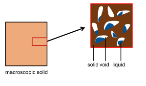
Figure 2.1: Partially saturated porous medium.

In this model, the heterogeneous body is considered as a continuous solid medium containing uniformly distributed small voids with a homogeneous porosity denoted by ${c}$. Upon interaction with a fluid, the fluid permeates into these small pores and diffuses within the medium, driven by the fluid concentration gradient, resulting in the creation of a mixture consisting of solid and fluid components, as illustrated in Figure 2.1.

2.1.1 Mass and momentum equations

With a porosity ${c}$ and fluid saturation level $\widetilde{c}$, as defined in reference [42], the locally effective fluid density $\rho^{l}$ can be expressed as

$$\rho^{l}=\rho^{L}\widetilde{c},$$ (1)

where $\rho^{L}$ is the fluid density. For a porous solid partially-saturated by fluid, the total linear momentum $\mathbf{M}$ in the region $\mathcal{R}$ is the sum of fluid momentum and solid momentum

$$\mathbf{M}=\rho\mathbf{v}=\rho^{l}\mathbf{v}^{l}+\rho^{s}\mathbf{v}^{s},$$ (2)

where $\rho$ and $\mathbf{v}$ are the total density and velocity respectively, $\mathbf{v}^{l}$ the velocity of fluid, $\rho^{s}$ and $\mathbf{v}^{s}$ the density and velocity of dry porous solid. Due to the difference between $\mathbf{v}^{l}$ and $\mathbf{v}^{s}$, the fluid flux $\mathbf{q}$ on the element boundary $\partial V$, considering a representative volume element $dV$, can then be expressed as

$$\mathbf{q}={\rho^{l}}(\mathbf{v}^{l}-\mathbf{v}^{s}).$$ (3)

Within an element $dV$ of the mixture, the momentum $\mathbf{M}$ is determined by both the stress exerted on the element and the fluid flux of linear momentum $\mathbf{v}^{l}\otimes\mathbf{q}$ on the boundary $\partial V$, where the symbol $\otimes$ means the outer product of two vectors or tensors. It follows that the conservation of total linear momentum of the mixture can be expressed as

$$\frac{d\mathbf{M}}{dt}=\nabla\cdot\bm{\sigma}-\nabla\cdot\left(\mathbf{v}^{l}\otimes\mathbf{q}\right),$$ (4)

where $\bm{\sigma}$ represents the Cauchy stress in the mixture acting on the solid. $\bm{\sigma}$ is determined by Cauchy stress $\bm{\sigma}^{s}$ due to deformation and the pressure stress $\bm{\sigma}^{l}$ resulting from the presence of the fluid phase, which is elaborated in Appendix A.2.

2.1.2 Fick’s law

In a partially saturated solid, variations in fluid saturation drive fluid movement regions with higher fluid fraction to those with lower fractions, and the resulting flux follows the Fick’s law as

$$\mathbf{q}=-D\rho^{l}\nabla\widetilde{c},$$ (5)

indicating that the fluid flux is proportional to the diffusivity $D$, the effective fluid density $\rho^{l}$, as well as the gradient of the fluid saturation $\widetilde{c}$. Consequently, the time derivative of fluid mass within an element $dV$ is attributed to the fluid flux $\mathbf{q}$ across the element boundary $\partial V$, considering Eq. (1), written as

$$\frac{d\rho^{l}}{dt}=-\nabla\cdot\mathbf{q}=D\rho^{L}\nabla\cdot(\widetilde{c}\leavevmode\nobreak\ \nabla\widetilde{c})=\frac{1}{2}D\rho^{L}\nabla^{2}\widetilde{c}^{2}.$$ (6)

where the second-derivative operator $\nabla^{2}$ defines the time derivative of fluid density.

2.2 Cardiac function

Following Chi’s algorithm [43], a model for simulating the principle aspects of cardiac function, including cardiac electrophysiology, passive mechanical response and electromechanical coupling is proposed. In this scenario, the anisotropic transmembrane potential propagation behavior of the myocardium is simulated by using our present anisotropic SPH diffusion discretization algorithm to achieve higher accuracy.

2.2.1 Kinematics and governing equations

In this section, we firstly concisely introduce the fundamental physical concepts of solid deformation, along with the relevant notations and symbols within the total Lagrange framework. Our analysis considers a solid body $\mathcal{B}$ that occupies two regions: $\mathcal{R}_{0}$ and $\mathcal{R}$, representing the body configurations at time $t_{0}$ (where $t=0$) and $t$, respectively. In the initial configuration $\mathcal{R}_{0}$, the position vector of a material point is denoted by $\mathbf{X}\in\mathcal{R}_{0}$, while in the current configuration $\mathbf{x}\in\mathcal{R}$. The motion of the solid body, represented by the invertible mapping $\phi$, transforms a material point $\mathbf{X}$ to its corresponding vector $\mathbf{x}=\phi(\mathbf{X},t)$, as shown in Figure 2.2. Accordingly, the Lagrangian velocity of a material point is given by $\mathbf{v}(\mathbf{X},t)=\frac{d\phi(\mathbf{X},t)}{dt}$. The deformation gradient $\mathbf{F}$, which characterizes the deviation of a material point from its initially undeformed position to its deformed position, can be calculated from the displacement vector $\mathbf{u}=\mathbf{x}-\mathbf{X}$ by the following equation:

$$\mathbf{F}=\frac{d\mathbf{x}}{d\mathbf{X}}=\nabla^{0}{\mathbf{u}}+\mathbf{I},$$ (7)

where $\nabla^{0}$ denotes the gradient operator defined in the initial reference configuration, $\mathbf{I}$ the unit matrix. The corresponding Jacobian determinant term $J=$ det($\mathbf{F}$) indicates the local volume gain $J>1$ or loss $J<1$.

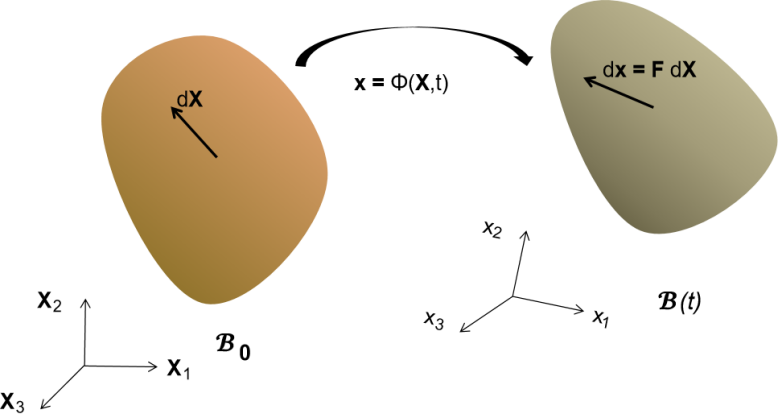
Figure 2.2: Finite deformation process on a body $\mathcal{B}$.

The governing equations of solid deformation within the total Lagrange framework are derived as

$$\begin{cases}\rho={\rho^{0}}\frac{1}{J}\\ \rho^{0}\frac{\text{d}\mathbf{v}}{\text{d}t}=\nabla^{0}\cdot\mathbf{P}^{T}\end{cases},$$ (8)

where $\rho$ and $\rho_{0}$ are the densities in the current configuration $\mathcal{R}$ and the initial configuration $\mathcal{R}_{0}$, respectively, $\mathbf{v}$ the velocity and $\mathbf{P}$ the first Piola-Kirchhoff stress tensor.

Considering a coupled system of cardiac electrophysiology and microelectronics following the total Lagrangian formulations [43]. The cardiac electrophysiology runs the principle of the evolution of the transmembrane potential $V_{m}$, expressed as

$$C_{m}\frac{dV_{m}}{dt}=\nabla^{0}\cdot(\mathbf{D}\nabla^{0}V_{m})+I_{ion},$$ (9)

where $C_{m}$ is the capacity of the membrane cell and $I_{ion}$ the ionic current. The conductivity tensor is defined by

$$\mathbf{D}=d^{iso}\mathbf{I}+d^{ani}\mathbf{f^{0}}\otimes\mathbf{f^{0}}$$ (10)

where $d^{iso}$ represents the isotropic contribution and $d^{ani}$ the anisotropic contribution to account for conductivity along the fiber direction $\mathbf{f^{0}}$. To close equations, the constitutive laws for the ionic current $I_{ion}$ and the first Piola–Kirchhoff stress $\mathbf{P}$ are required.

2.2.2 Constitutive equations

Referring to the approaches described in Refs.[44, 45], a so-called reduced-ionic model is implemented for the ionic current. Specifically, we utilize the Aliev–Panfilov model, where $I_{ion}(V_{m},w)$ is considered as a function of the transmembrane potential $V_{m}$ and the gating variable $w$, which indicates the percentage of open channels per unit area of the membrane. Particularly suitable for applications where electrical activity of the heart is the main interest, the Aliev–Panfilov model reads [45]

$$\left\{\begin{array}[]{l}I_{ion}\left(V_{m},w\right)=-kV_{m}\left(V_{m}-a\right)\left(V_{m}-1\right)-wV_{m}\\ \frac{\mathrm{d}w}{\mathrm{\leavevmode\nobreak\ d}t}=g\left(V_{m},w\right)=\epsilon\left(V_{m},w\right)\left(-kV_{m}\left(V_{m}-b-1\right)-w\right)\end{array},\right.$$ (11)

where $\epsilon\left(V_{m},w\right)=\epsilon_{0}+\mu_{1}w/\left(\mu_{2}+V_{m}\right)\text{ and }k,a,b,\epsilon_{0},\mu_{1}\text{ and }\mu_{2}$ are constant parameters. Note that dimensionless variables are employed here. The actual transmembrane potential $\tilde{V}_{m}$ measured in millivolts (mV) and time measured in milliseconds (ms) can be derived through scaling transformations, expressed as follows

$$\tilde{V}_{m}=100V_{m}-80.$$ (12)

2.2.3 Cardiac electromechanics

The first Piola–Kirchhoff stress $\mathbf{P}$ in Eq. (8) can be decomposed into passive $\mathbf{P}_{passive}$ and active response $\mathbf{P}_{active}$, expressed as [46]

$$\mathbf{P}=\mathbf{P}_{passive}+\mathbf{P}_{active}.$$ (13)

The passive first Piola–Kirchhoff stress $\mathbf{P}_{passive}$, characterizes the stress necessary to achieve a specified deformation of the passive myocardium, computed as

$$\mathbf{P}_{passive}=\mathbf{F}\mathbf{S},$$ (14)

where by adopting the Holzapfel–Ogden model [47] and incorporating the anisotropic characteristics of the myocardium, the second Piola–Kirchhoff stress $\mathbf{S}$ is defined as

$$\mathbf{S} =a\exp\left[b\left(I_{1}-3\right)\right]\mathbf{I}+\{\lambda\ln J-a\}\mathbf{C}^{-1}$$ (15)

$$+2a_{f}\left(I_{ff}-1\right)\exp\left[b_{f}\left(I_{ff}-1\right)^{2}\right]\mathbf{f}^{0}\otimes\mathbf{f}^{0}$$

$$+2a_{s}\left(I_{ss}-1\right)\exp\left[b_{s}\left(I_{ss}-1\right)^{2}\right]\mathbf{s}^{0}\otimes\mathbf{s}^{0}$$

$$+a_{fs}I_{fs}\exp\left[b_{fs}\left(I_{fs}\right)^{2}\right]\left(\mathbf{f}^{0}\otimes\mathbf{s}^{0}+\mathbf{s}^{0}\otimes\mathbf{f}^{0}\right)$$

where a, b, $a_{f}$, $b_{f},a_{s},b_{s},a_{fs}$ and $b_{fs}$ are eight positive material constants, with the $a$ parameters having dimension of stress and $b$ parameters being dimensionless. Here, $\lambda$ is Lamé parameter and $\mathbf{C}$ the left Cauchy–Green deformation tensor, expressed as

$$\mathbf{C}=\mathbf{F}^{T}\cdot\mathbf{F}$$ (16)

which possesses principal invariants, given by

$$I_{1}=\operatorname{tr}(\mathbf{C}),\quad I_{2}=\frac{1}{2}\left[I_{1}^{2}-\operatorname{tr}\left(\mathbf{C}^{2}\right)\right],\quad I_{3}=\operatorname{det}(\mathbf{C})=J^{2}.$$ (17)

Additionally, there are three other independent invariants that account for directional preferences:

$$I_{ff}=\mathbf{C}:\mathbf{f}^{0}\otimes\mathbf{f}^{0},\quad I_{ss}=\mathbf{C}:\mathbf{s}^{0}\otimes\mathbf{s}^{0},\quad I_{fs}=\mathbf{C}:\mathbf{f}^{0}\otimes\mathbf{s}^{0},$$ (18)

where $\mathbf{f}^{0}$ and $\mathbf{s}^{0}$ represent the undeformed myocardial fiber and sheet unit directions, respectively. The structure-based invariants $I_{ff}$ and $I_{ss}$ correspond to the isochoric fiber and sheet stretch squared, representing the squared lengths of the deformed fiber and sheet vectors, i.e., $\mathbf{f}=\mathbf{F}\mathbf{f}^{0}$ and $\mathbf{s}=\mathbf{F}\mathbf{s}^{0}$, and $I_{fs}$ signifies the fiber-sheet shear [47].

The active component $\mathbf{P}_{active}$, represents the tension produced by the depolarization associated with the propagating transmembrane potential, which is aligned with the fiber direction and is represented mathematically as [46]

$$\mathbf{P}_{active}={T}_{a}\mathbf{F}\mathbf{f}^{0}\otimes\mathbf{f}^{0},$$ (19)

with ${T}_{a}$ being the active cardiomyocite contraction stress, which evolves according to an ordinary differential equation (ODE) given by

$$\frac{\mathrm{d}T_{a}}{\mathrm{\leavevmode\nobreak\ d}t}=\epsilon\left(V_{m}\right)\left[k_{a}\left(V_{m}-V_{r}\right)-T_{a}\right],$$ (20)

where parameters $k_{a}$ and $V_{r}$ control the maximum active force, the resting transmembrane potential and the activation function [48]

$$\epsilon\left(V_{m}\right)=\epsilon_{0}+\left(\epsilon_{\infty}-\epsilon_{-\infty}\right)\exp\left\{-\exp\left[-\xi\left(V_{m}-\bar{V}_{m}\right)\right]\right\},$$ (21)

where $\epsilon_{-\infty}$ and $\epsilon_{\infty}$ are the limiting values as $V_{m}\rightarrow-\infty$ and $V_{m}\rightarrow\infty$. The parameters $\bar{V}_{m}$ and $\xi$ represent the phase shift and the transition slope, respectively, ensuring a smooth activation of the muscle contraction.

3 Theory of ASPH

Derived from smoothed particle hydrodynamics (SPH) method, the adaptive smoothed particle hydrodynamics (ASPH) method is predicated on an integral formulation, wherein pertinent physical quantities are approximated via the integration of neighboring particles, but the kernel function being evolved is adaptive. Spherical kernels of radius given by a scalar smoothing length in SPH is replaced by an anisotropic smoothing involving ellipsoidal kernels in ASPH. The real position vector is generalized to a normalized vector. This can be portrayed as a localized, linear shift of coordinates, which is described by a transformation tensor $\mathbf{G}$. This shift transforms the coordinates to a system where the anisotropic volume changes appear uniform in all directions.

3.1 Fundamental and theory of ASPH

Following Ref. [49], the real position vector $\bm{r}$, is generalized to a normalized form $\bm{\eta}$ in ASPH through a linear coordinate transformation tensor $\mathbf{G}$. This transformation is expressed as $\bm{\eta}=\mathbf{G}\bm{r}$, resulting in the representation of the kernel function $W(\bm{\eta})=W(\mathbf{G}\bm{r})$. In contrast to the isotropic kernel, the normalization undergoes a change: SPH: $\bm{\eta}=\bm{r}/h\rightarrow$ ASPH: $\bm{\eta}=\mathbf{G}\bm{r}$. It is evident that SPH can be regarded as a degenerate case of ASPH, where the tensor $\mathbf{G}$ becomes diagonal with a constant component of $1/h$.

Under such notations, the gradient of the kernel function $\nabla W(\bm{\eta})$ can be expressed as [49]

$$\nabla W(\bm{\eta})=\nabla W^{\prime}(\mathbf{G}\bm{r})=\dfrac{\partial W(\mathbf{G}\bm{r})}{\partial\bm{r}}=\dfrac{\partial\bm{\eta}}{\partial\bm{r}}\dfrac{\partial W}{\partial\bm{\eta}}=\mathbf{G}\frac{\bm{\eta}}{\eta}\dfrac{\partial W}{\partial\bm{\eta}},$$ (22)

Incorporating the particle summation, one has the approximation of derivative of a variable field $f$ at particle $i$ in a weak form by

$$\nabla f_{i}=\nabla f_{i}-f_{i}\nabla 1\approx-2\sum_{j}||\mathbf{G}||V_{j}\widetilde{f}_{ij}\nabla_{i}W_{ij},$$ (23)

and a strong form as

$$\nabla f_{i}=f_{i}\nabla 1+\nabla f_{i}\approx\sum_{j}||\mathbf{G}||V_{j}{f}_{ij}\nabla_{i}W_{ij},$$ (24)

where $V_{j}$ is the volume of the $j$-th neighboring particle, $\widetilde{f}_{ij}=(f_{i}+f_{j})/2$ is the inter-particle average value, $f_{ij}=f_{i}-f_{j}$ is the inter-particle difference value.

Considering a spatially varying smoothing tensor, the kernel function needs to be symmetrized to ensure the conservation of quantities such as linear momentum. The symmetrization of kernel function $W_{ij}$ and the gradient of which between two particles $i$ and $j$ can be implemented as the averaged formalism as

$$W_{ij}=\frac{1}{2}(W(\bm{\eta}_{i,ij})+W(\bm{\eta}_{j,ij})),\quad\nabla W_{ij}=\frac{1}{2}(\nabla W(\bm{\eta}_{i,ij})+\nabla W(\bm{\eta}_{j,ij})),$$ (25)

where

$$\bm{\eta}_{i,ij}=\mathbf{G}_{i}\bm{r}_{ij},\quad\bm{\eta}_{j,ij}=\mathbf{G}_{j}\bm{r}_{ij}.$$ (26)

3.2 Kernel function with nonisotropic smoothing

In the following cases, we use the Wenland kernel function and its first derivative which can be further written to match the nonisotropic ellipsoidal smoothing kernel as

$$W^{v-D}(\eta)=A^{v-D}\left\{\begin{array}[]{ll}(1-\frac{\eta}{2})^{4}(1+2\eta),&0\leq\eta\leq 2\\ 0,&\eta>2\end{array}\right.$$ (27)

$$\nabla W^{v-D}(\eta)=A^{v-D}\mathbf{G}\frac{\bm{\eta}}{\eta}\left\{\begin{array}[]{ll}-5\eta(1-\frac{\eta}{2})^{3},&0\leq\eta\leq 2\\ 0,&\eta>2\end{array}\right.$$ (28)

where $v$ means the dimension and

$$A^{1-D}=\frac{3}{4}||\mathbf{G}||,\quad A^{2-D}=\frac{7}{4\pi}||\mathbf{G}||,\quad A^{3-D}=\frac{21}{16\pi}||\mathbf{G}||.$$ (29)

Benefiting from the tensor $\mathbf{G}$, the displacement between two particles is mapped to the generalized position vector $\bm{\eta}$, the norm of which is compared with the cutoff radius to calculate the kernel function and kernel gradient value. Using normalized position vector $\bm{\eta}$ rather than $\mathbf{r}/h$ in the discretization of quantities, the expression of dynamic equations in SPH and ASPH are identical.

3.2.1 Transformation tensor $\mathbf{G}$

Defined as a linear transformation that maps from real position space ($\mathbf{r}$) to normalized position space ($\bm{\eta}$), $\mathbf{G}$ is determined by the coupling of the geometrically scaling transformation and the rotational transformation, involving the smoothing lengths in different directions and the rotation angle of the axes deviated from the real frame. Detailed information can be found in B and the reference paper [49].

4 First and second derivatives in ASPH

4.1 Correction of the first derivatives

To discretize the solid mechanics, we employ the initial undeformed configuration as the reference. First, aiming to restore the 1st-order consistency, the configuration of particle $i$ is corrected with a tensor $\mathbf{B}$ in the total Lagrangian formalism, expressed as [50, 51]

$$\mathbf{F}^{0}_{i}=\left(\sum_{j}V_{j}\left(\mathbf{r}^{0}_{j}-\mathbf{r}^{0}_{i}\right)\otimes\nabla^{0}_{i}W_{ij}\right)\mathbf{B}^{0}_{i}=\mathbf{I},$$ (30)

where $\bm{r}^{0}_{i}$ and $\bm{r}^{0}_{j}$ denote the positions of particles $i$ and $j$ in the reference configuration. Equivalently,

$$\mathbf{I}=\sum_{j}V_{j}\left(\mathbf{r}^{0}_{j}-\mathbf{r}^{0}_{i}\right)\otimes(\nabla^{0^{T}}_{i}W_{ij}\mathbf{B}^{0}_{i})=\sum_{j}V_{j}\left(\mathbf{r}^{0}_{j}-\mathbf{r}^{0}_{i}\right)\otimes(\mathbf{B}^{0^{T}}_{i}\nabla^{0}_{i}W_{ij})^{T}.$$ (31)

The gradient correction $\mathbf{B}$ is operated over $\nabla^{0}$ to correct the kernel. We define

$$\tilde{\nabla}^{0}=\mathbf{B}^{0^{T}}_{i}\nabla^{0},$$ (32)

where the symbol $\tilde{\nabla}^{0}_{i}$ represents the corrected approximation of the differential operator with respect to the initial material coordinates. From Eq. 30, involving the tensor $\mathbf{G}$, the correction matrix $\mathbf{B}^{0}$ of particle $i$ in ASPH can be consequently calculated as:

$$\mathbf{B}^{0}_{i}=\left(\sum_{j}V_{j}\left(\bm{r}^{0}_{j}-\bm{r}^{0}_{i}\right)\otimes\nabla^{0}_{i}W_{ij}\right)^{-1}=\left(\sum_{j}V_{j}\left(\bm{r}^{0}_{j}-\bm{r}^{0}_{i}\right)\otimes(\mathbf{G}_{i}\frac{\bm{\eta_{ij}}}{\eta_{ij}}\frac{\partial W}{\partial\eta_{ij}})\right)^{-1}.$$ (33)

In total Lagrangian formulation, the neighborhood of particle $i$ is defined in the initial configuration, and this set of neighboring particles remains fixed throughout the entire simulation. Therefore, $\mathbf{B}^{0}_{i}$ is computed only once under the initial reference configuration.

4.2 Second derivatives coupling with nonisotropic resolution

Considering the diffusion in a thin structure, with large aspect ratio, it is favorable to discretize the computation domain with nonisotropic resolution to reduce total particle number, as shown in Figure. 4.1. To cope with this nonisotropic resolution, we apply a nonisotropic kernel, where an ellipsoid smoothing replaces the normal sphere one, as shown in Figure. 1(b).

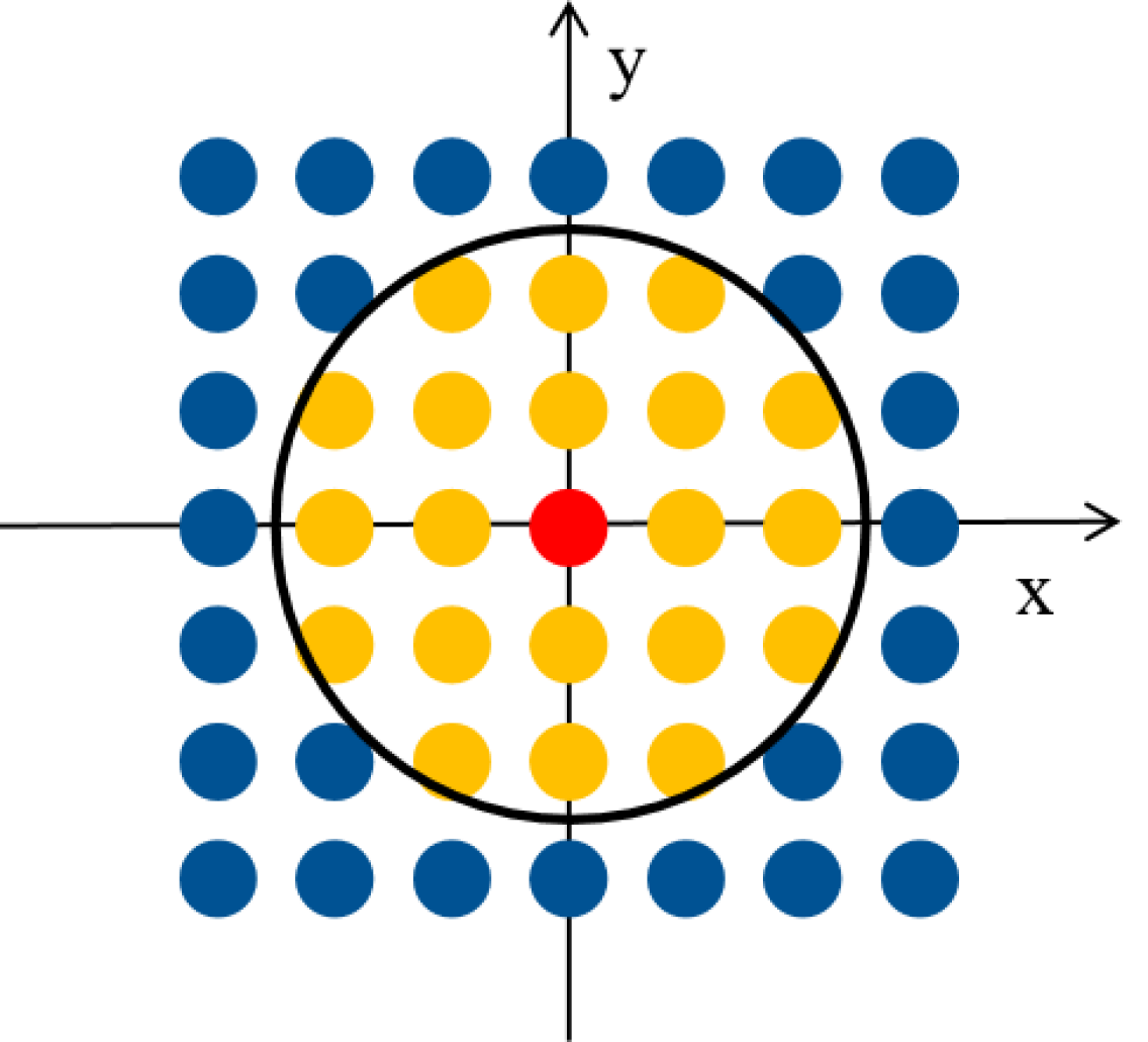
(a)

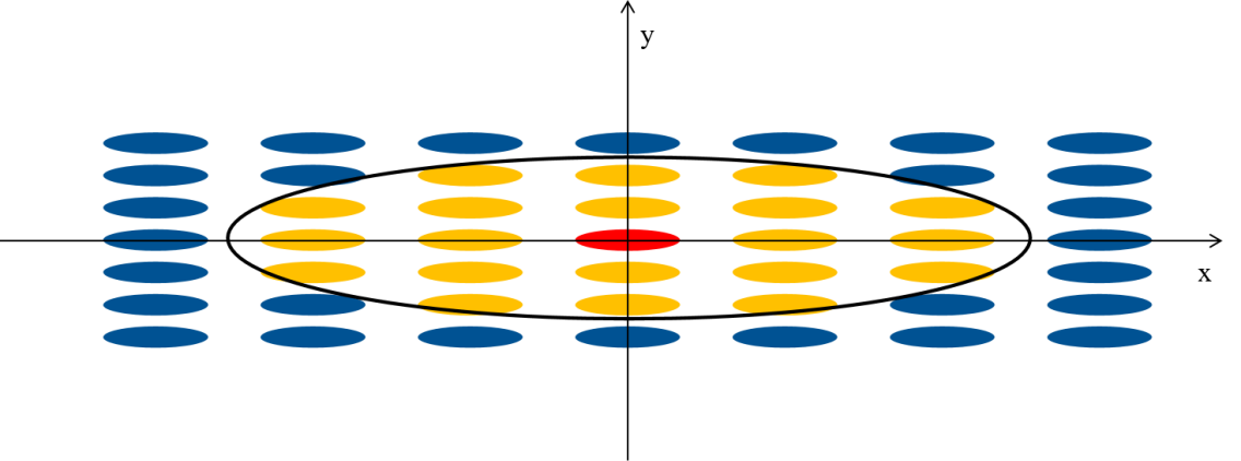
(b)

Figure 4.1: (a) Isotropic with spherical smoothing kernel and (b) anisotropic resolutions with elliptical smoothing kernel.

With the nonisotropic resolution, presenting the Taylor series expansion of function at $x_{i}$ in $\bm{x}$-coordinate which is nonisotropic, there is

$$\phi_{i}=\phi_{j}+\frac{\partial\phi}{\partial\bm{x}}\cdot\bm{r}_{ij}+\frac{1}{2}\bm{r}_{ij}\cdot\frac{\partial^{2}\phi_{i}}{\partial\bm{x}^{2}}\bm{r}_{ij}+R_{(3)}=\phi_{j}+\frac{\partial\phi}{\partial\bm{x}}\cdot\bm{r}_{ij}+R_{(2)},$$ (34)

where $\phi_{j}$ means the value of $\phi$ at particle $j$ and $\bm{r}_{ij}$ means the particle distance vector between particle $i$ and particle $j$, the $R_{(2)}$ and $R_{(3)}$ represent the truncation error of first and second order, respectively. Consequently,

$$\phi_{ij}:=\phi_{i}-\phi_{j}=\nabla\phi_{i}\cdot\bm{r}_{ij}+R_{(2)},$$ (35)

where

$$R_{(2)} \approx\frac{1}{2}r_{ij}\cdot\frac{\partial^{2}\phi_{i}}{\partial x^{2}}r_{ij}$$ (36)

$$=\frac{1}{2}\sum_{{\mathrm{i}}=1}^{\text{ndim }}\sum_{{\mathrm{j}}=1}^{\text{ndim}}r^{\mathrm{i}}_{ij}r^{\mathrm{j}}_{ij}\frac{\partial^{2}\phi_{i}}{\partial x^{\mathrm{i}}\partial x^{\mathrm{j}}}.$$

where the term with superscript $r^{\mathrm{i}}_{ij}$ and $r^{\mathrm{j}}_{ij}$ mean the components of the vector $\bm{r}_{ij}$.

Following Asai Mitsuteru [41], in total Lagrangian formulation, the term $\nabla\phi$ in the right hand of Eq. (35) at particle $i$ can be approximated in SPH as

$$\langle\nabla\phi_{i}\rangle_{(2)} =\bigcup_{j\in\mathbb{S}^{i}}\frac{m_{j}}{\rho_{j}}\tilde{\nabla}^{0}_{i(\bm{x})}W_{ij}\left(\phi_{i}-\phi_{j}-R_{(2)}\right)$$ (37)

$$\approx\bigcup_{j\in\mathbb{S}^{i}}\frac{m_{j}}{\rho_{j}}\tilde{\nabla}^{0}_{i(\bm{x})}W_{ij}\left(\phi_{i}-\phi_{j}-\frac{1}{2}\sum_{{\mathrm{i}}=1}^{\text{ndim }}\sum_{{\mathrm{j}}=1}^{\text{ndim}}r^{\mathrm{i}}_{ij}r^{\mathrm{j}}_{ij}\frac{\partial^{2}\phi_{i}}{\partial x^{\mathrm{i}}\partial x^{\mathrm{j}}}\right),$$

satisfying the second order accuracy. Note that $\tilde{\nabla}^{0}_{i(\bm{x})}W_{ij}$ is the gradient kernel approximated in the nonisotropic ${\bm{x}}$-coordinate with kernel correction matrix $\mathbf{B}^{0}$ applied, written as $\tilde{\nabla}^{0}_{i(\bm{x})}W_{ij}=\mathbf{B}^{0^{T}}\mathbf{G}_{i}\frac{\bm{\eta_{ij}}}{\eta_{ij}}\frac{\partial W}{\partial\eta_{ij}}$. Consequently, by applying Eq. (37) and Eq. (36) to Eq. (35),

$$\phi_{i}-\phi_{j} \approx\bm{r}_{ij}\cdot\langle\nabla\phi_{i}\rangle_{(2)}+\frac{1}{2}\sum_{{\mathrm{i}}=1}^{\text{ndim }}\sum_{{\mathrm{j}}=1}^{\text{ndim}}r^{\mathrm{i}}_{ij}r^{\mathrm{j}}_{ij}\frac{\partial^{2}\phi_{i}}{\partial x^{\mathrm{i}}\partial x^{\mathrm{j}}}$$ (38)

$$\approx\bm{r}_{ij}\cdot\left\{\bigcup_{k\in\mathbb{S}^{i}}\frac{m_{k}}{\rho_{k}}\tilde{\nabla}^{0}_{i(\bm{x})}W_{ik}\left(\phi_{i}-\phi_{k}-\frac{1}{2}\sum_{{\mathrm{i}}=1}^{\text{ndim }}\sum_{{\mathrm{j}}=1}^{\text{ndim}}r^{\mathrm{i}}_{ik}r^{\mathrm{j}}_{ik}\frac{\partial^{2}\phi_{i}}{\partial x^{\mathrm{i}}\partial x^{\mathrm{j}}}\right)\right\}$$

$$\ \qquad\qquad\qquad\qquad+\frac{1}{2}\sum_{{\mathrm{i}}=1}^{\text{ndim }}\sum_{{\mathrm{j}}=1}^{\text{ndim}}r^{\mathrm{i}}_{ij}r^{\mathrm{j}}_{ij}\frac{\partial^{2}\phi_{i}}{\partial x^{\mathrm{i}}\partial x^{\mathrm{j}}}.$$

It can be transformed to

$$\left[\begin{array}[]{l}\left\langle\frac{\partial^{2}\phi_{i}}{\left(\partial x^{1}\right)^{2}}\right\rangle_{(2)}\\ \left\langle\frac{\partial^{2}\phi_{i}}{\left(\partial x^{2}\right)^{2}}\right\rangle_{(2)}\\ \left\langle\frac{\partial^{2}\phi_{i}}{\left(\partial x^{3}\right)^{2}}\right\rangle_{(2)}\\ 2\left\langle\frac{\partial^{2}\phi_{i}}{\partial x^{1}\partial x^{2}}\right\rangle_{(2)}\\ 2\left\langle\frac{\partial^{2}\phi_{i}}{\partial x^{2}\partial x^{3}}\right\rangle_{(2)}\\ 2\left\langle\frac{\partial^{2}\phi_{i}}{\partial x^{3}\partial x^{1}}\right\rangle_{(2)}\end{array}\right]=2\mathbf{M}^{-1}\ \bigcup_{j\in\mathbb{S}^{i}}\left[\frac{m_{j}}{\rho_{j}}\frac{\bm{r}_{ij}\cdot\tilde{\nabla}^{0}_{\bm{x}}W_{ij}}{\left|\bm{r}_{ij}\right|^{4}}\left\{\phi_{ij}-\bm{r}_{ij}\cdot\left(\bigcup_{k\in\mathbb{S}^{i}}\frac{m_{k}}{\rho_{k}}\phi_{ik}\tilde{\nabla}^{0}_{\bm{x}}W_{ik}\right)\right\}\mathbf{s}_{ij}\right],$$ (39)

where $\mathbf{s}_{ij}=[({r^{1}_{ij}})^{2},\ ({r^{2}_{ij}})^{2},\ ({r^{3}_{ij}})^{2},\ r^{1}_{ij}r^{2}_{ij},\ r^{2}_{ij}r^{3}_{ij},\ r^{3}_{ij}r^{1}_{ij}]^{T}$, and

$$\mathbf{M}_{i}^{\mathrm{(i,j,k,l)}}=\bigcup_{j\in\mathbb{S}^{i}}\frac{m_{j}}{\rho_{j}}\frac{\bm{r}_{ij}\cdot\tilde{\nabla}^{0}_{\bm{x}}W_{ij}}{\left|\bm{r}_{ij}\right|^{4}}\left\{(r_{ij}^{\mathrm{i}}\ r_{ij}^{\mathrm{j}}\ r_{ij}^{\mathrm{k}}\ r_{ij}^{\mathrm{l}})-(r_{ij}^{\mathrm{i}}\ r_{ij}^{\mathrm{j}})\bm{r}_{ij}\cdot\bigcup_{k\in\mathbb{S}^{i}}\frac{m_{k}}{\rho_{k}}(r_{ik}^{\mathrm{k}}\ r_{ik}^{\mathrm{l}})\tilde{\nabla}^{0}_{\bm{x}}W_{ik}\right\}$$ (40)

Accordingly, the diffusion rate of $\phi$ at particle $i$ is obtained by

$$\langle\frac{\partial\phi_{i}}{\partial t}\rangle_{(2)}=\left\langle\frac{\partial^{2}\phi_{i}}{\left(\partial x^{1}\right)^{2}}\right\rangle_{(2)}+\left\langle\frac{\partial^{2}\phi_{i}}{\left(\partial x^{2}\right)^{2}}\right\rangle_{(2)}+\left\langle\frac{\partial^{2}\phi_{i}}{\left(\partial x^{3}\right)^{2}}\right\rangle_{(2)},$$ (41)

which has the second order accuracy, while in two dimensional case, it is simplified to

$$\langle\frac{\partial\phi_{i}}{\partial t}\rangle_{(2)}=\left\langle\frac{\partial^{2}\phi_{i}}{\left(\partial x^{1}\right)^{2}}\right\rangle_{(2)}+\left\langle\frac{\partial^{2}\phi_{i}}{\left(\partial x^{2}\right)^{2}}\right\rangle_{(2)}.$$ (42)

4.3 Nonisotropic diffusion with nonisotropic diffusion coefficients

Considering the diffusion equation

$$\frac{\partial c}{\partial t}=\nabla\cdot(\mathbf{D}\nabla c),$$ (43)

where $c$ is the concentration function and $\mathbf{D}$ is the diffusion coefficient tensor, which is commonly influenced by the material properties or the geometry of the computational domain and so on, behaving nonisotropic features, expressed by a symmetric positive-definite tensor. In the case, the $\mathbf{D}$ is written as

$$\mathbf{D}=\begin{bmatrix}D_{11}&D_{12}&D_{13}\\ D_{21}&D_{22}&D_{23}\\ D_{31}&D_{32}&D_{33}\end{bmatrix}.$$ (44)

Usually, in an isotropic diffusion case, $\mathbf{D}$ is considered to be a scalar diffusion coeffici ent as [33]

$$(\nabla\cdot(\mathbf{D}\nabla c))_{i}=2\sum_{j}V_{j}{D}\frac{c_{ij}}{r_{ij}}\frac{\partial W_{ij}}{\partial r_{ij}},$$ (45)

where $c_{ij}=c_{i}-c_{j}$. In anisotropic cases, $\mathbf{D}$ is considered to be a symmetric positive-definite matrix and can be decomposed by Cholesky decomposition as [17],

$$\mathbf{D}=\mathbf{L}\mathbf{L}^{\mathbf{T}}.$$ (46)

By changing the coordinate

$$\mathbf{X}=\mathbf{L}^{-1}\mathbf{x},$$ (47)

the original nonisotropic diffusion operator is transformed to be isotropic in $\mathbf{X}$-coordinate system as

$$\nabla\cdot(\mathbf{D}\nabla c)=\nabla_{\mathbf{X}}\cdot(\nabla_{\mathbf{X}}c)=(\nabla\cdot\nabla)_{\mathbf{X}}c.$$ (48)

Since there is a Hessian matrix formulation as

$$\mathbf{H}_{X}=\begin{bmatrix}\vspace{1.3ex}\frac{\partial^{2}\phi_{i}}{\left(\partial X^{1}\right)^{2}}&\frac{\partial^{2}\phi_{i}}{\partial X^{1}\partial X^{2}}&\frac{\partial^{2}\phi_{i}}{\partial X^{1}\partial X^{3}}\\ \vspace{1.3ex}\frac{\partial^{2}\phi_{i}}{\partial X^{2}\partial X^{1}}&\frac{\partial^{2}\phi_{i}}{\left(\partial X^{2}\right)^{2}}&\frac{\partial^{2}\phi_{i}}{\partial X^{2}\partial X^{3}}\\ \vspace{1.3ex}\frac{\partial^{2}\phi_{i}}{\partial X^{3}\partial X^{1}}&\frac{\partial^{2}\phi_{i}}{\partial X^{3}\partial X^{2}}&\frac{\partial^{2}\phi_{i}}{\partial X^{3}\partial X^{2}}\end{bmatrix},\leavevmode\nobreak\ \leavevmode\nobreak\ \mathbf{H}_{x}=\begin{bmatrix}\vspace{1.3ex}\frac{\partial^{2}\phi_{i}}{\left(\partial x^{1}\right)^{2}}&\frac{\partial^{2}\phi_{i}}{\partial x^{1}\partial x^{2}}&\frac{\partial^{2}\phi_{i}}{\partial x^{1}\partial x^{3}}\\ \vspace{1.3ex}\frac{\partial^{2}\phi_{i}}{\partial x^{2}\partial x^{1}}&\frac{\partial^{2}\phi_{i}}{\left(\partial x^{2}\right)^{2}}&\frac{\partial^{2}\phi_{i}}{\partial x^{2}\partial x^{3}}\\ \vspace{1.3ex}\frac{\partial^{2}\phi_{i}}{\partial x^{3}\partial x^{1}}&\frac{\partial^{2}\phi_{i}}{\partial x^{3}\partial x^{2}}&\frac{\partial^{2}\phi_{i}}{\partial x^{3}\partial x^{2}}\end{bmatrix},$$ (49)

while obviously $\mathbf{H}_{X}=\mathbf{L}\leavevmode\nobreak\ \mathbf{H}_{x}\leavevmode\nobreak\ \mathbf{L}^{T}$. According to Eq. (80) in C, the elements of Hessian matrix $\mathbf{H}_{x}$ can be concluded from the full expression of the second derivative model. Therefore, applying the relation of $\mathbf{H}_{X}=\mathbf{L}\leavevmode\nobreak\ \mathbf{H}_{x}\leavevmode\nobreak\ \mathbf{L}^{T}$, the Laplacian with nonisotropic diffusion tensor coefficient can be obtained by

$$\nabla\cdot(\mathbf{D}\nabla c)=(\nabla\cdot\nabla c)_{\mathbf{X}}=\frac{\partial^{2}\phi_{i}}{\left(\partial X^{1}\right)^{2}}+\frac{\partial^{2}\phi_{i}}{\left(\partial X^{2}\right)^{2}}+\frac{\partial^{2}\phi_{i}}{\left(\partial X^{3}\right)^{2}}.$$ (50)

5 ASPH discretization

5.1 ASPH discretization for fluid-structure interaction

In the fluid-structure interaction model discretization, each particle carries the location $\mathbf{x}_{n}=\phi(\mathbf{X},t_{n})$ at time $t_{n}$, along with an initial representative volume $V^{0}$ that partitions the initial domain of the macroscopic solid. The deformation gradient $\mathbf{F}_{n}$ of the solid phase is stored to update the solid current volume $V_{n}$ and density $\rho^{s}_{n}$. Additionally, the fluid mass $m_{n}^{l}$, saturation $\widetilde{a}_{n}$, and density-weighted velocity of the fluid relative to solid $\mathbf{q}_{n}$ are stored. The fluid mass equation Eq. (6) of particle $i$ is discretized as

$$\frac{\text{d}m_{i}^{l}}{\text{d}t}=2V_{i}\sum_{j}\frac{m_{j}}{\rho_{j}}(\mathbf{q}_{i}-\mathbf{q}_{j})\tilde{\nabla_{i}}W_{ij}.$$ (51)

Note that with the Eq (7), we have the relation of gradient kernel function in the total Lagrangian and updated Lagrangian $\tilde{\nabla_{i}}W_{ij}=\mathbf{B}^{0^{T}}_{i}\mathbf{F}^{-1}\nabla_{i}^{0}W_{ij}$. Once fluid mass is updated, the locally effective fluid density $\rho^{l}$ is obtained subsequently. According to Eq. (1) and Eq. (5), we update the fluid saturation $\widetilde{a}$ and the fluid flux $\mathbf{q}$ in the particle form

$$\mathbf{q}_{i}=-K\rho^{l}V_{i}\sum_{j}\frac{m_{j}}{\rho_{j}}(\widetilde{c}_{i}-\widetilde{c}_{j})\tilde{\nabla_{i}}W_{ij}.$$ (52)

With the fluid flux and the stress in hand, we obtain discrete formulations for the momentum balance Eq. (4) as

$$\frac{d\mathbf{M}_{i}}{dt}=2\sum_{j}V_{j}(\bm{\sigma}_{i}+\bm{\sigma}_{j})\tilde{\nabla_{i}}W_{ij}-2\sum_{j}V_{j}({\mathbf{v}_{i}^{l}\otimes\mathbf{q}_{i}}+{\mathbf{v}_{j}^{l}\otimes\mathbf{q}_{j}})\tilde{\nabla_{i}}W_{ij},$$ (53)

where $\bm{\sigma}_{i}$ and $\bm{\sigma}_{j}$ are the stress tensors of particles $i$ and $j$. We then compute the updated solid velocity $\mathbf{v}^{s}$ using the total momentum definition Eq. (2), where the total density of the mixture is the sum of the solid and fluid densities $\rho=\rho^{s}+\rho^{l}$, written as

$$\mathbf{v}^{s}=\frac{\mathbf{M}-\mathbf{q}}{\rho}=\frac{\mathbf{M}-\mathbf{q}}{\rho^{s}+\rho^{l}}.$$ (54)

Subsequently, the fluid velocity $\mathbf{v}^{l}$ is calculated using Eq. (3) as

$$\mathbf{v}^{l}=\mathbf{v}^{s}-\frac{\mathbf{q}}{\rho^{l}}.$$ (55)

5.2 ASPH discretization of cardiac function

The anisotropic ASPH discretization of diffusion is given in section 4.3. For the discretization of momentum equation, considering the kernel correction, Eq. (8) can be approximated in the weak form as

$$\frac{d\mathbf{v}_{i}}{{d}t}=\frac{2}{\rho_{i}}\sum_{j}V_{j}\tilde{\mathbf{P}}_{ij}{\nabla}^{0}_{i}W_{ij},$$ (56)

where $\rho_{i}$ represents the density of particle $i$, $\tilde{\mathbf{P}}_{ij}$ is the averaged first Piola-Kirchhoff stress of the particle pair $(i,j)$, and to keep the conservative of particles, the correction matrix $\mathbf{B}^{0^{T}}$ is performed on each particle, thus $\tilde{\mathbf{P}}_{ij}$ is stated as

$$\tilde{\mathbf{P}}_{ij}=\frac{1}{2}\left(\mathbf{P}_{i}\mathbf{B}^{0^{T}}_{i}+\mathbf{P}_{j}\mathbf{B}^{0^{T}}_{j}\right).$$ (57)

The first Piola-Kirchhoff stress tensor is dependent on the deformation tensor $\mathbf{F}$, referring to Eq. (30), the time derivative of which is computed from

$$\frac{d\mathbf{F}_{i}}{dt}=\left(\sum_{j}V_{j}\left(\mathbf{v}_{j}-\mathbf{v}_{i}\right)\otimes\nabla^{0}_{i}W_{ij}\right)\mathbf{B}^{0}_{i}.$$ (58)

6 Numerical examples

6.1 Diffusion with nonisotropic resolution

In this section, we discretize the computation with different anisotropic ratios to form nonisotropic resolutions. Firstly, the second-order accuracy of the algorithm is verified by comparing the result generated by the current method with the analytical solution. Subsequently, a block diffusion coupling with periodic boundary conditions is tested. Finally, the fluid-solid interaction model is simulated to show the applicability of this algorithm.

6.1.1 Verification of second-derivative operator in a square patch

Considering a square patch composed of a number of SPH particles, and according to its position, each particle receives the values of the following function

$$\phi(x,y)=x^{2}+y^{2},\leavevmode\nobreak\ \leavevmode\nobreak\ 0\leq x,\leavevmode\nobreak\ y\leq 1$$ (59)

and the analytical solution of this function is

$$\frac{d\phi(x,y)}{dt}=\frac{\partial^{2}\phi}{\partial x^{2}}+\frac{\partial^{2}\phi}{\partial y^{2}}=4.$$ (60)

The numerical value $\frac{d\phi}{dt}$ is evaluated on the particles that compose the square patch. Figure. LABEL: shows the contour obtained from the analytical solution and the present ASPH method with different ratios $r$ = 1.0, 2.0, 4.0, 8.0. Regardless of the anisotropic ratios, all results precisely correspond to the analytical solution, demonstrating the algorithm’s accuracy.

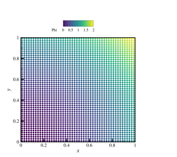
(a) $\phi$ distribution.

(b) The analytical solution of $\frac{d\phi}{dt}$ .

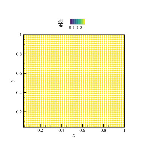
(c) The ASPH method with r = 1.0.

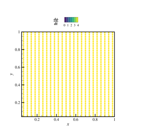
(d) The ASPH method with r = 2.0.

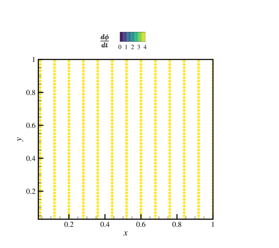
(e) The ASPH method with r = 4.0.

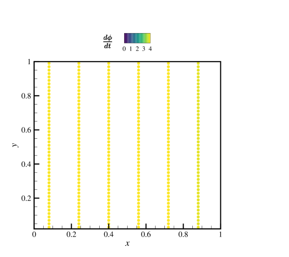
(f) The ASPH method with r = 8.0.

Figure 6.1: 2D nonoisotropic diffusion: comparisons of the $\frac{d\phi}{dt}$ contour obtained from (a) the analytical solution and (b)-(f) the present ASPH method with different anisotropic ratios.

6.1.2 Diffusion in a rectangle

For a more complex initial condition, Considering the a two-dimensional rectangle with a dimensionless length of 1 and width of 0.1, with a initial physical parameter $\phi$ setup as

$$\phi=\{\begin{array}[]{ll}1.0,&0.4\leq x\leq 0.6\\ 0,&\rm else\end{array}$$ (61)

The dimensionless diffusion coefficient $D$ is set as 1.0. Neumann boundary conditions are applied. The diffusion is simulated by the present ASPH algorithm and various anisotropic ratios are settled to compare the efficiency.

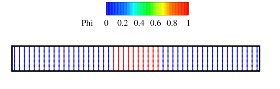
(a) t = 0.

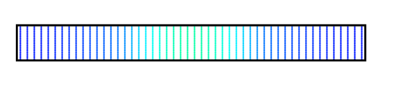
(b) t = 0.02.

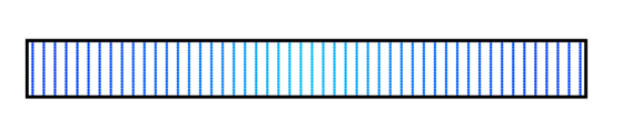
(c) t = 0.04.

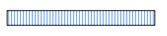
(d) t = 0.2.

Figure 6.2: Diffusion in a rectangle: the time evolution of $\phi$ contour at different time instants using ASPH with anisotropic ratio r = 4.0, $N_{y}$ = 20.

Using the ASPH method with anisotropic ratio $r$ = 4.0, particle number in $y$ direction (the vertical direction) $N_{y}$ = 20, Figure 6.2 illustrates snapshots of the diffusion at different time instances. We record the $\phi$ value across the horizontal line of $y$ = 0.05, and diffusion process at different time instances yielded by the ASPH algorithm with different $r$ are depicted in Figure. 6.3. With the analytical solution being $\phi$ = 0.1 throughout the domain at the final stable state, very close results are obtained by using SPH and ASPH algorithm with various anisotropic ratios. The convergence study is performed, taking r = 4.0 as example, as particle number increases, the final stable result of $\phi$ are converged to the analytical solution being 0.1 throughout the domain. To quantitatively verify the accuracy, the normalized root mean square error (RMSE) is evaluated between the analytical solution and the numerical values computed by the second-derivative operator, defined as

$$\rm{RMSE}\leavevmode\nobreak\ (\left<\phi\right>^{i})=\frac{\sqrt{\sum_{i}(\phi^{i}-\left<\phi\right>^{i})^{2}}}{\sqrt{\sum_{i}(\phi^{i})^{2}}},$$ (62)

where $\phi^{i}$ indicates the analytical solution of these test functions, and $\left<\phi\right>^{i}$ is the numerical value derived from ASPH method. The normalized RMSE error comparison is shown in Figure. 6.4.

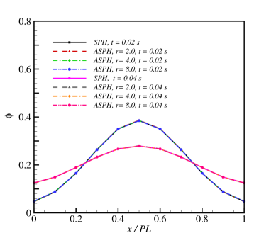
Figure 6.3: Diffusion in a rectangle: the $\phi$ variation on the horizontal line of the

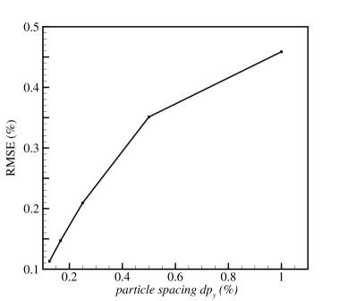
Figure 6.4: Diffusion in a rectangle: the RMSE error under different resolution with anisotropic ratio = 4.0.

6.1.3 Two dimensional fluid diffusion coupling solid deformation

In this section, we perform a two-dimensional simulation of fluid diffusion coupling with porous solid deformation to validate the efficiency of the presented method. As illustrated in Figure. 6.5, a thin porous beam with a length of $L$ = 5.0 mm and width of $W$ = 0.125 mm is considered. The left and right sides are constrained to prevent any curling or movement. The simulation starts with a fluid droplet contacting the center part of the beam, extending to a length of $0.3L$. The total physical time is set to 500 seconds. Given the slender nature of the beam, we assume that initially, all pores in the upper half part are filled with fluid. As mentioned earlier, the relationship between fluid saturation $\widetilde{c}$ and solid porosity ${c}$ is $0\leq\widetilde{c}\leq{c}<1$. For this 2D and 3D cases discussed later, we assume a solid porosity of ${c}=0.4$, implying that the fluid saturation $\widetilde{c}$ in the central part($0.5W\times 0.3L$) is constrained to $\widetilde{c}={c}=0.4$ initially, while in other regions $\widetilde{c}_{0}=0.0$.

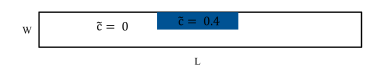
Figure 6.5: 2D fluid-structure interaction: physical configuration of the thin porous beam.

In alignment with the experimental setup, the solid material is modeled as a porous and elastic Nafion membrane, with water serving as the fluid. The physical properties and material parameters of this membrane are listed in Table 6.1. The pressure coefficient C has been calibrated to fit the experimentally measured flexure curves, while other parameters are obtained from previous research papers [52, 53].

Table 6.1: Fluid-structure interaction: physical material parameters value of Nafion film. Data estimated from Motupally and Goswami [52, 53].

Parameters	$\rho$ ${\rm(kg/m^{3})}$	$D$ ${\rm(m^{2}/s)}$	Pressure coefficient C ${\rm(MPa)}$	Young modulus ${\rm(MPa)}$	Poisson ratio
Value	2000	$1.0\times 10^{-10}$	$3.0$	$8.242$	0.2631

In the simulation, considering the thin nature, the anisotropic resolution is applied when discretizing the computation domain. Firstly, four particles are placed in the vertical direction, with a vertical particle spacing of $dp_{y}=W/6=2.08\times 10^{-2}$ mm. Different anisotropic ratios $r=2.0,\leavevmode\nobreak\ 4.0,\leavevmode\nobreak\ 6.0$ are applied, resulting in the horizontal particle spacing as $dp_{x}=2.0\leavevmode\nobreak\ dp_{y},\leavevmode\nobreak\ 4.0\leavevmode\nobreak\ dp_{y},\leavevmode\nobreak\ 6.0\leavevmode\nobreak\ dp_{y}$.

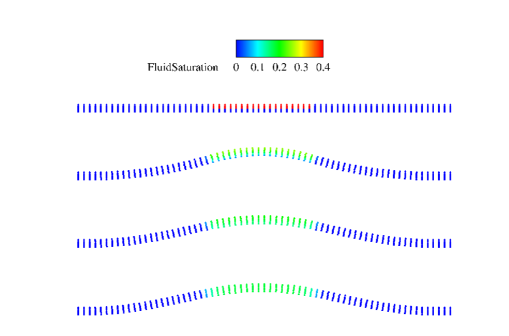
Figure 6.6: 2D fluid-structure interaction: the physical configuration with anisotropic ratio = 4.0 colored by the fluid saturation at different time instants, from up to down, $t=0,\leavevmode\nobreak\ 100\leavevmode\nobreak\ 200,\leavevmode\nobreak\ 500$ s.

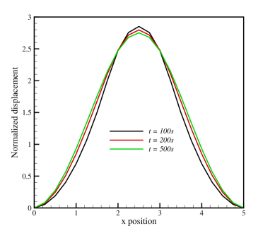
Figure 6.7: 2D fluid-structure interaction: the vertical normalized displacement $y/PH$ versus the horizontal $x$ position with anisotropic ratio = 4.0 at different time instants, from up to down, $t=0,\leavevmode\nobreak\ 100\leavevmode\nobreak\ 200,\leavevmode\nobreak\ 500$ s.

With the specified conditions, the simulation produces a deformed configuration colored by fluid saturation, illustrated in Figure. 6.6. Initially, the presence of a water droplet in the upper central region induces fluid pressure, as explained in Eq. 6.7, leading to a localized bending in the central region. As time progresses, the saturation difference drives continuous water diffusion, showing a smooth transition from the center to the surrounding area. Figure. 6.7 depicts the vertical normalized displacement $y/PH$ versus the horizontal $x$ position of the beam at different time instants. As a more uniform pressure distribution develops, a smoother flexure of the beam is obtained in the later period.

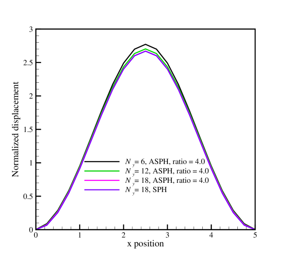
(a) The comparison of normalized displacement.

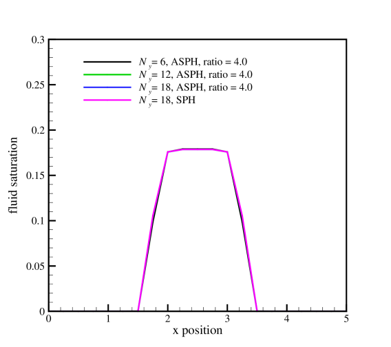
(b) The comparison of saturation $\widetilde{c}$.

Figure 6.8: 2D fluid-structure interaction: comparisons of the vertical normalized displacement $y/PH$ (a) and the saturation (b) versus the horizontal $x$ position obtained from the ASPH solution with anisotropic ratio = 4.0 under different resolutions to the converged results from SPH method.

To test the accuracy, we refine the particle resolution to perform the convergence test. Taking the anisotropic ratio r = 4.0 as an example, we maintain $r$ constant while varying the total particle with different particle distribution densities $N_{y}$ = H/$dp_{y}$ = 6, 12, 18, with $dp_{x}$ = 4$dp_{y}$. Figure. 6.8 shows the final vertical normalized displacement $y/PH$ and the saturation $\widetilde{c}$ distributions versus the horizontal $x$ position of the beam by applying the isotropic SPH method and the present ASPH with ratio = 4.0 under different resolutions. With increasing particle density, the disparity in $y/PH$ and $\widetilde{c}$ between different resolutions using ASPH method diminishes, indicating a convergence pattern. Additionally, the converged outcomes derived from ASPH with $r$ being 4.0 and SPH are visually indistinguishable in both the final vertical normalized displacement $y/PH$ and $\widetilde{c}$ distribution of the beam, validating the reliability of the ASPH method in simulating diffusion problems in thin structures.

The efficiency of the proposed approach is demonstrated through Table 6.2, providing a quantitative comparison of the present ASPH method against the SPH approach in terms of particle number N, computation time t as well as the normalized root mean square error (RMSE) of saturation $\widetilde{c}$ at the final time instant. The root mean square error (RMSE) is defined as

$$\rm{RMSE}\leavevmode\nobreak\ (\left<\widetilde{c}\right>^{i})=\frac{\sqrt{\sum_{i}(\widetilde{c}^{i}-\left<\widetilde{c}\right>^{i})^{2}}}{\sqrt{\sum_{i}(\widetilde{c}^{i})^{2}}},$$ (63)

where $\widetilde{c}^{i}$ indicates the converged solution, and $\left<\widetilde{c}\right>^{i}$ is a numerical value related to $\widetilde{c}$ evaluated by SPH and ASPH methods. From this table, it can be inferred that the present ASPH method reduces both the number of particles and the computational time. Despite small deviations existing among different ASPH ratios, the results from ASPH are all very close to the converged results from SPH method, with the difference no exceeding 4%, while achieving notable time savings.

Table 6.2: 2D fluid-structure interaction: quantitative comparison of the accuracy and efficiency of this present ASPH algorithm with different anisotropic ratios.

Method	$N$	$t\leavevmode\nobreak\ (s)$	Time saved	$\rm{RMSE}\leavevmode\nobreak\ (\left<\widetilde{c}\right>^{i})$
SPH	1482	$655.5$	-	$0.00388$
ASPH ratio = 2.0	761	$398.1$	39.2%	$0.00985$
ASPH ratio = 4.0	402	$233.9$	64.2%	$0.02267$
ASPH ratio = 6.0	282	$147.7$	77.5%	$0.03847$

6.1.4 Three dimensional fluid diffusion coupling solid deformation

Next, we explore fluid diffusion coupling swelling in a three-dimensional film, specifically the diffusion of water within a porous Nafion membrane. This system has been previously investigated numerically by Zhao [42] and experimentally by Goswami [53]. This reference thin porous body takes the form of a polymer film with an x-y plane of dimensions $L_{x}=10.0$ mm, $L_{y}=10.0$ mm and a height of $L_{z}=0.125$ mm. Four boundary sides are constrained to prevent any curling or movement. The physical parameters are consistent with those listed in Table 6.1, and the initial conditions resemble those employed in the two-dimensional case. The central square part of the membrane in contact with water occupies a region of dimensions $0.3L_{x}\times 0.3L_{y}\times 0.5L_{z}$, and this contact lasts for 450 seconds, with the total physical time set to 2500 seconds. No fluid is allowed to diffuse out from the membrane. The fluid saturation $\widetilde{c}$ in the central square part is constrained to $\widetilde{c}={c}=0.4$ for the initial 450 seconds, while in other regions $\widetilde{c}_{0}=0$. In order to provide a more accurate representation of the experiment, the evaporation process is taken into consideration, acknowledging the gradual loss of water over time. During the initial period, deformation and flexure manifest, and subsequently, as the fluid mass diminishes from the membrane, a gradual restoration of the original shape is observed.

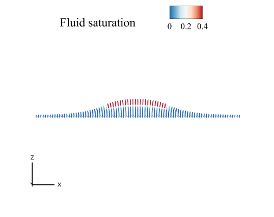
(a) t = 450s, front view

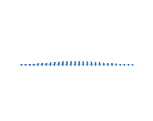
(b) t = 1500s, front view

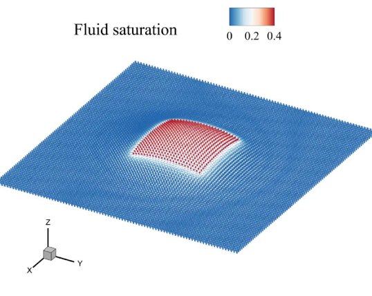
(c) t = 450s, top side view

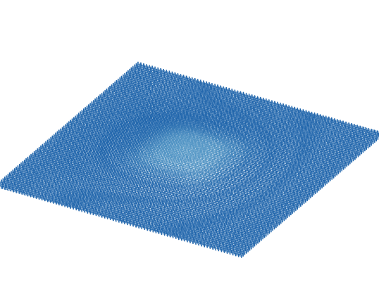
(d) t = 1500s, top side view

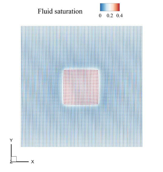
(e) t = 450s, top view

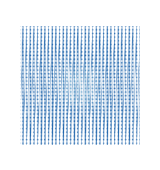
(f) t = 1500s, top view

Figure 6.9: 3D fluid-structure interaction: the deformation colored by fluid saturation at different time instants.

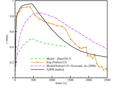
Figure 6.10: 3D fluid-structure interaction: bending amplitude of the center point compared with experimental data and results from other numerical models.

Figure 6.9 illustrates membrane deformation colored by water saturation at different time instants, indicating the diffusion evolution within the membrane. Figure 6.10 depicts the swelling degree $z$ of the central point versus different time instants, which are derived from the present method as well as other numerical models and the corresponding data points from Goswami’s experimental measurements [53]. The numerical simulation results obtained from the present ASPH method exhibit good agreement with experimental results, capturing the deformation amplitude pattern, reproducing the increasing flexure during the water contact period and the subsequent decrease after the contact phase, consistent with saturation variations.

6.2 Nonisotropic diffusion with anisotropic diffusion tensor

In many cases, diffusion processes in the real problems are directionally dependent or anisotropic. In this section, simulations for a contaminant source diffusing in water are firstly carried out, and the results are compared with the corresponding analytical solutions to demonstrate the accuracy. Then the cardiac function coupling with nonisotropic diffusion is simulated to verify the application of this method to complex biological problems.

6.2.1 2d source diffusion

In this section, we consider a contaminant source in water, which has been studied by Tran-Duc et al. [17] with numerical and analytical results available to compare with. The contaminant source is located in the center of a square computation domain spanning dimensions of 200 m × 200 m. Throughout the simulation, the initial contaminant spatial distributions are generated utilizing analytical solutions detailed as

$$C(x,t)=\frac{1}{4\pi t\prod_{\alpha=1}^{2}\sqrt{\mathbf{D}_{\alpha\alpha}}}\prod_{\alpha=1}^{2}\exp\left[-\frac{\left(x_{\alpha}-x_{\alpha,0}\right)^{2}}{4t\mathbf{D}_{\alpha\alpha}}\right],$$ (64)

at a temporal instance of t = 120 s (2 min). Subsequently, the contaminant distributions following 30 minutes of diffusion are juxtaposed against corresponding analytical solutions. Spatial resolution, denoted as the particle spacing, is set at x= 0.5 m. Consequently, the respective quantities of SPH particles are determined to be 160,000. In the first case, the anisotropic diffusion tensor is

$$\mathbf{D}=\begin{bmatrix}0.1&0.0\\ 0.0&0.01\end{bmatrix}\rm{(m^{2}\leavevmode\nobreak\ s^{-1})},$$ (65)

in which diffusion rates in the x-direction surpasses that in the y-direction.

Figure 6.11 illustrates both the numerical and analytical distributions of time t = 1920 s. Generally, the concentration distributions exhibit elliptical shapes with the major axis aligned in the x-direction and the minor axis in the y-direction, which arises from the inherent discrepancy in diffusion rates between the x and y directions. Notably, a notable concordance is observed between the numerical solution and the analytical counterpart in both their shapes and value profiles.

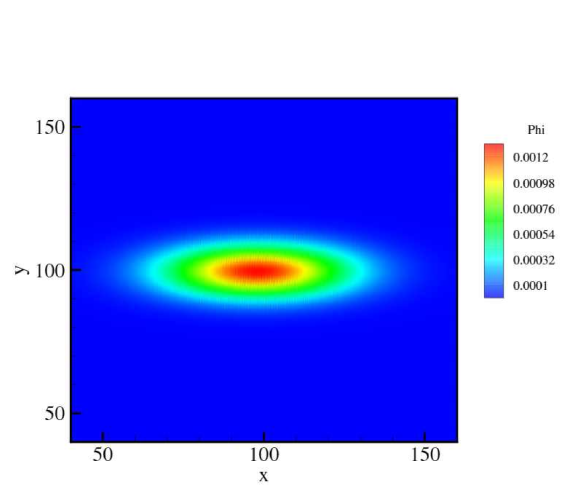
(a) The present ASPH method.

(b) The analytical solution.

Figure 6.11: 2D anisotropic diffusion: comparisons of the concentration distribution obtained from (a)the present ASPH method and (b) the analytical solution.

For a more rigorous comparison, the current numerical concentration distributions at a horizontal cross-section at y = 100 m (Figure. 12(a)) and a vertical cross-section at x = 100 m (Figure. 12(b)) are depicted, alongside a comparative analysis with analytical solutions and the results by Tran-Duc et al. [17] in Figure 4. The concentration profiles approximated through ASPHAD in the refer [17] is thinner in x-direction and more stretched in y-direction, while the current ASPH distribution demonstrate a more commendable agreement with the analytical solution. The current results mitigate the level of anisotropy inherent in the diffusion process, displaying an agreed anisotropy in comparison to the analytical solution.

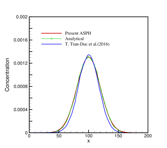
(a)

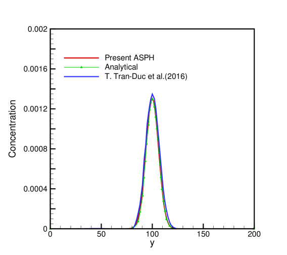
(b)

Figure 6.12: 2D anisotropic diffusion: comparisons of the concentration distribution of (a) a horizontal cross-section at y = 100 m (b) a vertical cross-section at x = 100 m.

In the subsequent test, we consider a more general case with a full diffusion tensor

$$\mathbf{D}=\begin{bmatrix}0.1&0.03\\ 0.03&0.03\end{bmatrix}\rm{(m^{2}\leavevmode\nobreak\ s^{-1})}.$$ (66)

The simulated concentration distribution portrayed in Figure. 6.13 exhibits a notable coherence with the analytical solution, evident in both shape and concentration values at time t = 1920 s. As anticipated, the concentration distributions of present ASPH has orientation but maintain an elliptical form as similar as the analytical distribution, which means that ASPH conserves the principal diffusing directions.

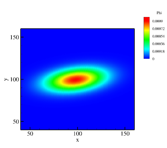
(a) The present ASPH method.

(b) The analytical solution.

Figure 6.13: 2D anisotropic diffusion: comparisons of the concentration distribution obtained from (a)the present ASPH method and (b) the analytical solution.

Figures. 14(a) and 14(b) present the current numerical concentration distributions as well as the analytical solution at the horizontal cross-section, specifically at x = 100 m, and the vertical cross-section at y = 100 m, respectively. Again, the ASPH demonstrates enhanced computational accuracy. while discernible reduction in the level of anisotropy is observed in the ASPHAD distribution when juxtaposed with previous findings.

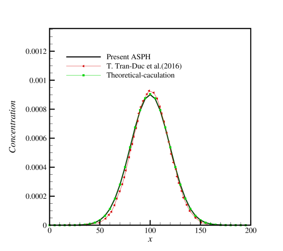
(a)

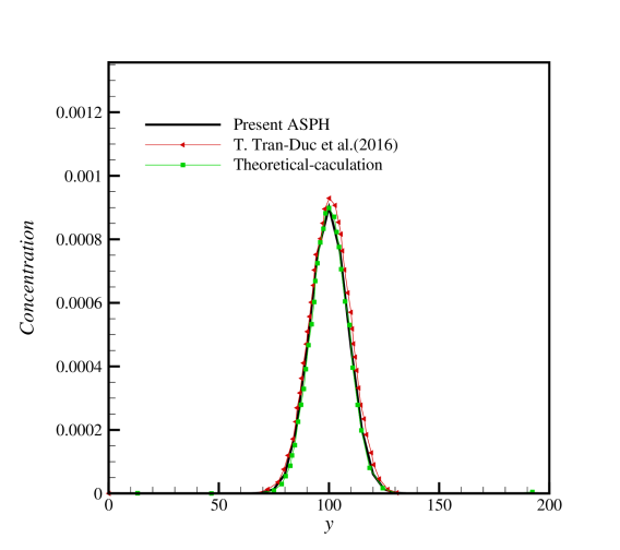
(b)

Figure 6.14: 2D anisotropic diffusion: comparisons of the concentration distribution of (a) a horizontal cross-section at y = 100 m (b) a vertical cross-section at x = 100 m.

6.2.2 Simulation of transmembrane potential propagation

The application of the present method is verified by a comprehensive example of heart, encompassing electrophysiology, passive mechanical response, and electromechanical coupling. Initially, we conduct benchmarking on the electrical activity of the heart.

Table 6.3: Transmembrane potential propagation: parameters in Aliev-Panfilov model.

k = 8.0	a = 0.15	b = 0.15	$\epsilon_{0}=0.034$	$\mu_{1}=0.2$	$\mu_{2}=0.3$

Using the work of Ratti and Verani [54] as our baseline, we consider a problem on the propagation of transmembrane potential to validate the accuracy of our method in solving the diffusion-reaction equations that describe electrophysiology. Assuming a two dimensional square domain of $(0,1)^{2}$ being isotropic, the nondimensional time interval is set equal to (0, 16). Being isotropic tissue, the nondimensional diffusion coefficients are $d_{iso}$ = 1.0 and $d_{ani}$ = 0.0. The transmembrane potential and gating variable are initialized by Eq. (67), where we apply the Aliev–Panfilov model with the constant parameters given in Table 6.3.

$$\begin{cases}V_{m}=\rm exp[-\frac{(x-1)^{2}+y^{2}}{0.25}]\\ w=0\end{cases}.$$ (67)

The sequential progression of the potential is displayed in Figure. 6.15. Figure. 6.16 reports the predicted evolution profile of the transmembrane potential at point (0.3, 0.7), and compares it values with the work of Ratti and Verani [54] and Rui et al. [55]. In accordance with the previous numerical estimation and experimental observation [44], our implementation accurately replicates the quick propagation of the stimulus in the tissue and the gradual decrease in transmembrane potential following a plateau phase.

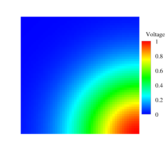
(a) t = 0.

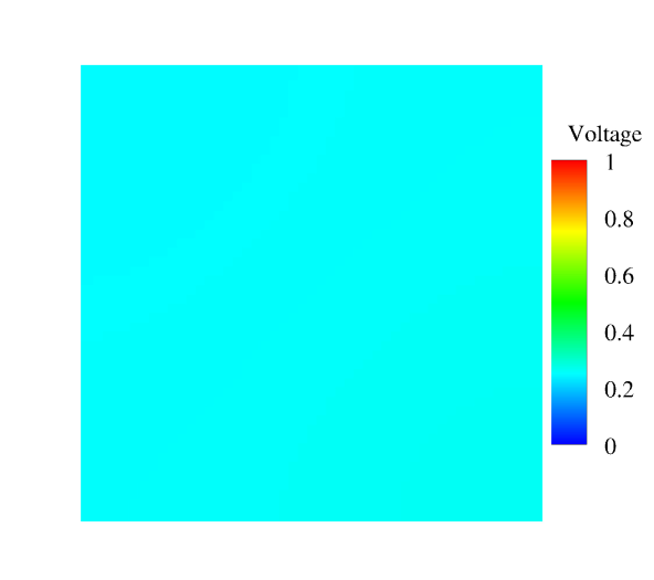
(b) t = 0.5.

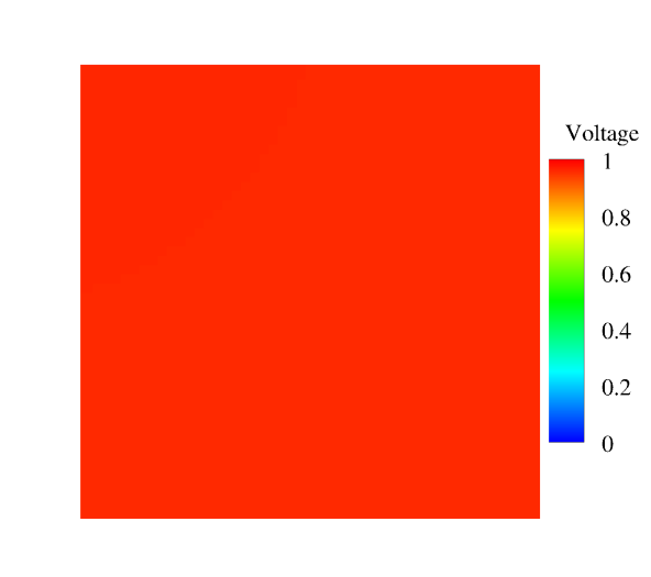
(c) t = 2.5.

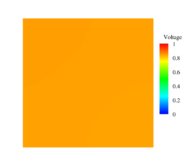
(d) t = 7.

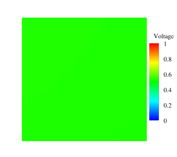
(e) t = 10.

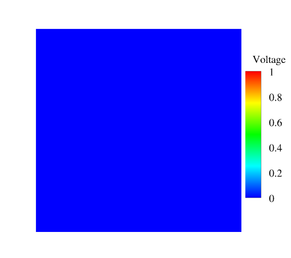
(f) t = 14.

Figure 6.15: Snapshots of the transmembrane potential evolution simulation.

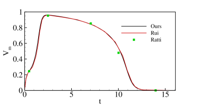
Figure 6.16: The time evolution of the transmembrane potential at point (0.3, 0.7), compared with the simulation results reported by Ratti and Verani [54] and Rui et al. [55].

6.2.3 3d cardiac function coupling with nonisotropic diffusion

To illustrate the capabilities of the current ASPH method in comprehensive cardiac simulations, we examine the propagation of transmembrane potentials as free pulses, along with the associated excitation-contraction dynamics within a three-dimensional left ventricle model. Building upon the work of [56, 57], the ionic current is modeled using the Aliev–Panfilow model with constant parameters given in Table. 6.5 and the diffusion coefficients are set as $d_{iso}$ = 0.8 mm²/ms and d_ani = 1.2 mm²/ms. For the momentum equation, Holzapfel–Ogden constitution model is employed, with parameters listed in Table. 6.4.

Table 6.4: 3d cardiac function: parameters in Holzapfel–Ogden constitution model.

$a=0.059$ kPa	$a_{f}=18.472$ kPa	$a_{s}=2.841$ kPa	$a_{fs}=0.216$ kPa
$b$ = 8.023	$b_{f}$ = 16.026	$b_{s}$ = 11.12	$b_{fs}$ = 11.436

Table 6.5: 3d cardiac function: parameters in the Aliev–Panfilov model.

$k$	$a$	$b$	$\epsilon_{0}$	$\mu_{1}$	$\mu_{2}$
8.0	0.01	$0.15$	0.002	0.2	0.23

The transmembrane potential travels in the left ventricle from the base to the apex, with a free-pulse stimulus applied at the muscular source for time interval $t\in[0,0.5]$ ms with a stimulation $V_{m}$ = 20 mV and the potential evolution is depicted in Figure. 6.17. It can be observed that the transmembrane potential propagates in the similar pattern for both iso- and anisotropic material model. Figure. 6.18 and Figure. 6.19 report the time evolution of the transmembrane potentials and the $z$ components of the displacements at the apex separately for both isotropic and anisotropic material models. Compared with the isotropic condition, the anisotropic one induces slightly slower propagation of the transmembrane potential in the ventricle and corresponding different mechanical response. For both isotropic and anisotropic materials, the transmembrane potential profiles show similar pattern to the results reported by Zhang et al. [56].

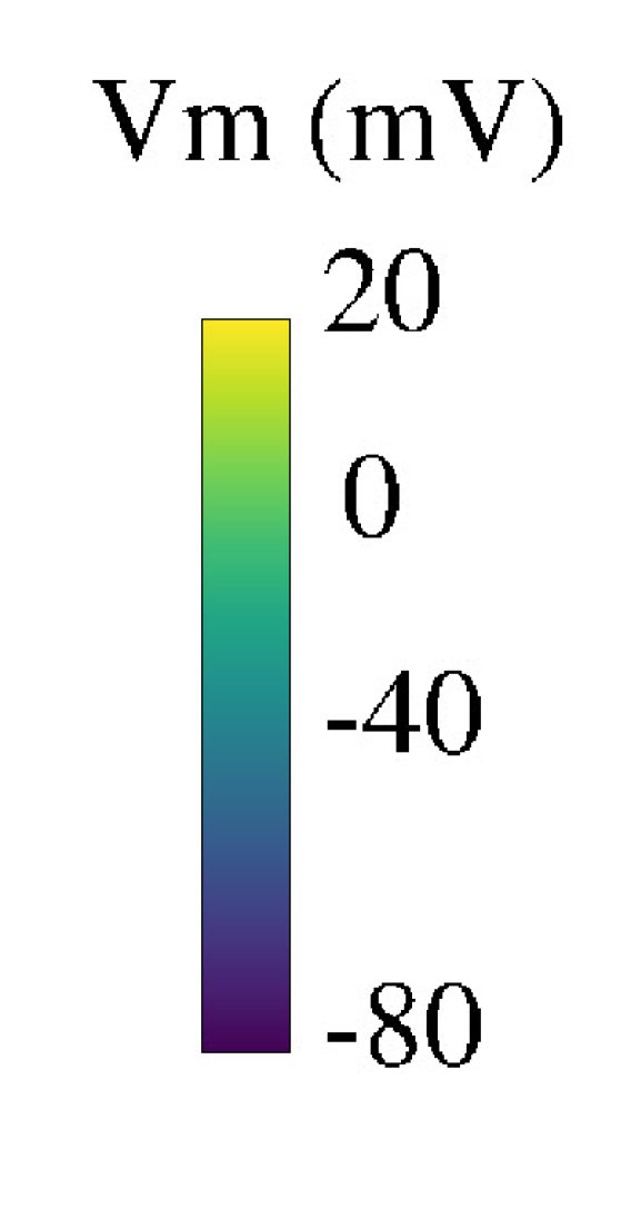
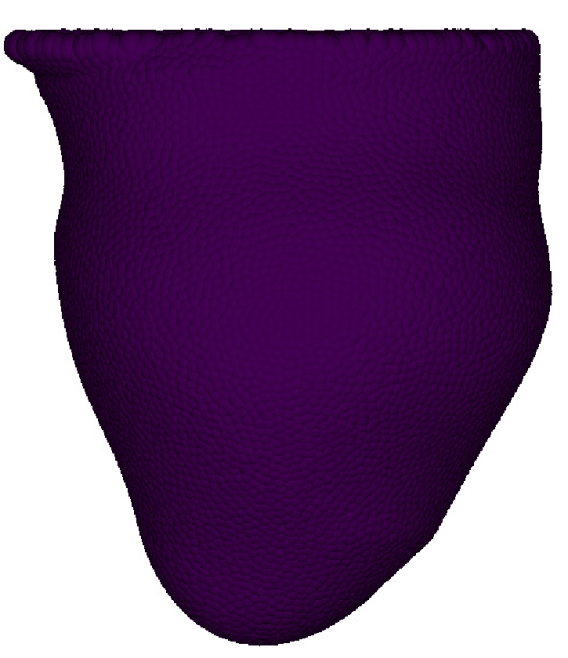
(a) t = 0 ms.

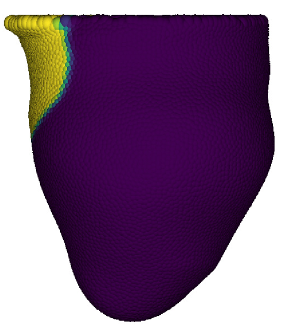
(b) t = 130 ms.

(c) t = 387 ms.

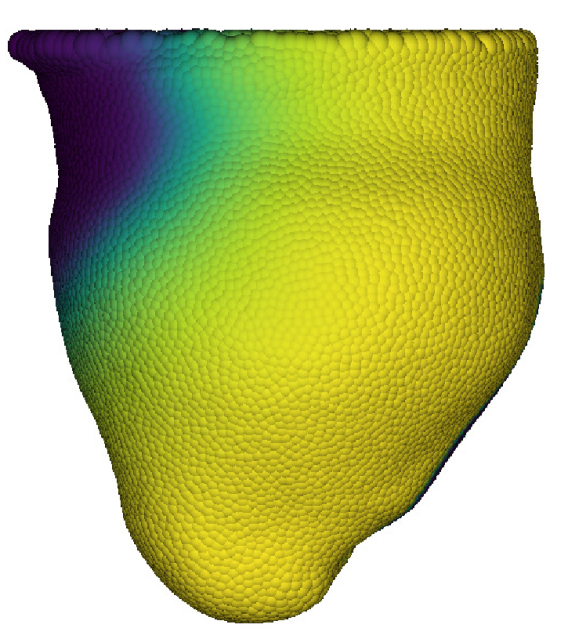
(d) t = 516 ms.

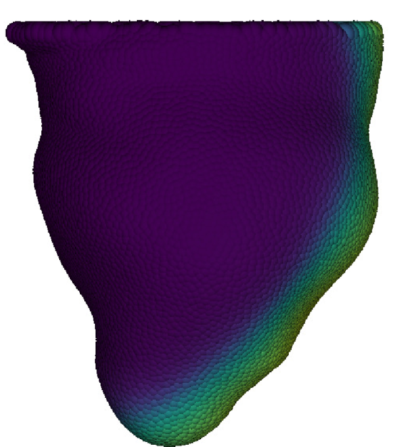
(e) t = 774 ms.

(f) t = 0 ms.

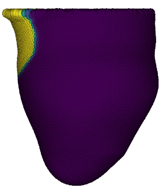
(g) t = 130 ms.

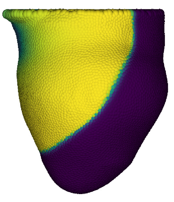
(h) t = 387 ms.

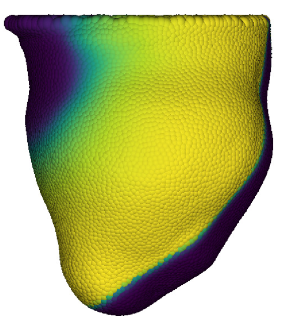
(i) t = 516 ms.

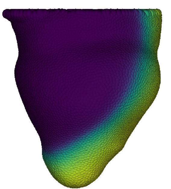
(j) t = 774 ms.

Figure 6.17: Left ventricle model: The propagation of the transmembrane potential in the heart triggering by a free-pulse pattern. The snapshots depict contours of the transmembrane potential $V_{m}$.

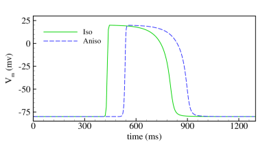
Figure 6.18: Left ventricle model: the time history of the transmembrane potential recorded on the apex.

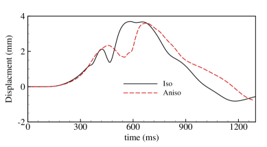
Figure 6.19: Generic biventricluar heart: the time history of displacement recorded on the apex.

7 Conclusion

In this study, we incorporate a second derivative model based on smooth particle hydrodynamics (SPH) to solve the diffusion process with anisotropic characteristics. A full-version formulation with second order accuracy that contains the elements of the hessian matrix is applied to deduce the diffusion operator. With the Hessian matrix in hand, a coordinate transformation tensor is applied to obtain the anisotropic diffusion operator. For diffusion in thin structures, anisotropic resolution coupling anisotropic kernel are employed to enhance the computation efficiency. Anisotropic kernel and gradient functions are considered when applying the Taylor series expansion to the second derivative model, producing the Laplacian operators.

The behavior of the present scheme was analyzed by applying it to typical diffusion problems with analytical solution, including the diffusion of scalar with pre-function within a thin structure and anisotropic diffusion of a contaminant contaminant in fluid. In both cases, the comparison with the theoretical solution demonstrating the present scheme can achieve the second order accuracy. Even with large ansiotropic characteristic,   the present method perfectly reproduces the analytical result. Convergence tests in terms of spatial resolution are also examined. Furthermore,  the application of the proposed SPH second derivative model to the diffusion in thin membrane and the anisotropic transport of transmembrane potential within the left ventricle have been conducted with promising results. Generally, the introduced ASPH formulations of the anisotropic Laplacian show improved performance when compared to classical SPH formulations, in terms of better approximation accuracy and higher stability. The non-physical values of the scalar quantities which are usually occur in other methods are effectively avoided, and the oscillations are eliminated. More comprehensive studies and detailed comparisons with traditional SPH method are needed to fully explore the advantages of present ASPH algorithm.

Appendix A Fluid-structure interaction model

In this appendix, we reference Zhao’s algorithm [42] to provide a concise overview of the porosity assumption for porous media model and its associated relations, including porosity and fluid saturation (A.1), as well as stress relations (A.2). In this mixture model, the definition of state variables including solid density $\rho^{s}$, locally fluid density $\rho^{l}$, solid velocity $\mathbf{v}^{s}$, and fluid saturation $\widetilde{c}$ enables the fluid velocity to be calculated with reference to the solid velocity. This simplified approach is practically significant, notably reducing the system complexity by eliminating the necessity for two separate sets of equations to describe the fluid and solid separately.

A.1 Porosity and fluid saturation

Considering a representative volume element $dV$, the macroscopic porosity $c$ is defined as the ratio of the total volume of the pores $dV^{p}$ to $dV$, yielding $c=\frac{dV^{p}}{dV}$. Note that $0<{c}<1$ holds for all cases. When the porous solid is partially saturated by fluid, the fluid saturation level $\widetilde{c}$ can be defined as

$$\widetilde{c}=\frac{dV^{l}}{dV},$$ (68)

where $dV^{l}$ denotes the fluid volume in the representative element $dV$. Clearly, $\widetilde{c}$ is always less than or equal to the maximum possible saturation ${c}$, i.e., $\widetilde{c}\leq{c}$. The locally effective fluid density $\rho^{l}$, defined as the mass of the fluid per unit volume, varies depending on the extent of fluid saturation and can be expressed as

$$\rho^{l}=\frac{dm^{l}}{dV}=\frac{dm^{l}}{dV^{l}}\frac{dV^{l}}{dV}=\rho^{L}\widetilde{c},$$ (69)

where $dm^{l}$ represents the mass of the fluid within $dV$, ${\rho}^{L}$ the fluid density which is assumed to be a constant for incompressible fluids.

A.2 Effective stress on solid

Following [58, 59, 60, 61], the total stress acting on the solid is the sum of Cauchy stress $\bm{\sigma}^{s}$ due to deformation and the pressure stress $\bm{\sigma}^{l}$ due to the presence of the fluid phase, written as:

$$\bm{\sigma}=\bm{\sigma}^{s}+\bm{\sigma}^{l}=\bm{\sigma}^{s}-p^{l}\mathbf{I}.$$ (70)

where $p^{l}$ is fluid pressure. For a hyper-elastic material, the constitutive equation for the solid component is given by

$$\bm{\sigma}^{s}=2\mu\mathbf{e}+\lambda\text{tr}(\mathbf{e})\mathbf{I},$$ (71)

where the Eulerian-Almansi finite strain tensor $\mathbf{e}$ can be evaluated by

$$\mathbf{e}=\frac{1}{2}(\mathbf{I}-\mathbf{F}^{T}\mathbf{F}).$$ (72)

The Lam$\acute{e}$ parameter $\lambda$ can be calculated via shear modulus $\mu$ and bulk modulus $K$ as $\lambda=K-\frac{2\mu}{3}$.

The fluid pressure solely depends on the fluid saturation level within the porous solid element, represented by a function $p^{l}=p^{l}(\widetilde{c})$. In the present model, this behavior is described mathematically by applying a linear relation, taking the form

$$p^{l}=C(\widetilde{c}-\widetilde{c}_{0}),$$ (73)

where $C$ is a material constant, $\widetilde{c}_{0}$ the initial saturation. Details can be referred to [61].

Appendix B Transformation tensor $\mathbf{G}$

For a two-dimensional case, with $h_{1}$ denoting the length in semimajor axis direction and $h_{2}$ in the semiminor axis in an ellipse, $\theta$ being the rotation angle of the semimajor axis compared to the real frame, $\mathbf{G}$ is given by,

$$\mathbf{G}=\begin{bmatrix}h_{1}^{-1}\cos^{2}\theta+h_{2}^{-1}\sin^{2}\theta&(h_{1}^{-1}-h_{2}^{-1})\cos\theta\sin\theta\\ (h_{1}^{-1}-h_{2}^{-1})\cos\theta\sin\theta&h_{1}^{-1}\sin^{2}\theta+h_{2}^{-1}\cos^{2}\theta\\ \end{bmatrix}.$$ (74)

If a kernel frame is consistent with the real frame, in other words, rotation angle $\theta=0$, $\mathbf{G}$ can be simplified into

$$\mathbf{G}=\begin{pmatrix}h_{1}^{-1}&0\\ 0&h_{2}^{-1}\\ \end{pmatrix}.$$ (75)

While for a more complex three-dimensional case, with a vector $(h_{1},h_{2},h_{3})$ representing the smoothing lengths along different axes in the kernel frame, and the rotation angle $(\omega,\psi,\chi)$ between the kernel frame and the real $(x,y,z)$ frames, $\mathbf{G}$ can be expressed as

$$\mathbf{G}=\begin{pmatrix}G_{11}&G_{21}&G_{31}\\ G_{21}&G_{22}&G_{32}\\ G_{31}&G_{32}&G_{33}\end{pmatrix},$$ (76)

where the six elements are defined as

$$\begin{array}[]{l}G_{11}=h_{1}^{-1}\omega_{1}^{2}\psi_{1}^{2}+h_{2}^{-1}\left(\omega_{1}\psi_{2}\chi_{2}-\omega_{2}\chi_{1}\right)^{2}+h_{3}^{-1}\left(\omega_{1}\psi_{2}\chi_{1}+\omega_{2}\chi_{2}\right)^{2},\\ \begin{split}G_{21}&=h_{1}^{-1}\omega_{1}\omega_{2}\psi_{1}^{2}+h_{2}^{-1}\left(\omega_{1}\psi_{2}\chi_{2}-\omega_{2}\chi_{1}\right)\left(\omega_{2}\psi_{2}\chi_{2}+\omega_{1}\chi_{1}\right)\\ &+h_{3}^{-1}\left(\omega_{2}\psi_{2}\chi_{1}-\omega_{1}\chi_{2}\right)\left(\omega_{1}\psi_{2}\chi_{1}+\omega_{2}\chi_{2}\right),\\ \end{split}\\ G_{31}=-h_{1}^{-1}\omega_{1}\psi_{1}\psi_{2}+h_{2}^{-1}\psi_{1}\chi_{2}\left(\omega_{1}\psi_{2}\chi_{2}-\omega_{2}\chi_{1}\right)+h_{3}^{-1}\psi_{1}\chi_{1}\left(\omega_{1}\psi_{2}\chi_{1}+\omega_{2}\chi_{2}\right),\\ G_{22}=h_{1}^{-1}\omega_{2}^{2}\psi_{1}^{2}+h_{2}^{-1}\left(\omega_{2}\psi_{2}\chi_{2}+\omega_{1}\chi_{1}\right)^{2}+h_{3}^{-1}\left(\omega_{2}\psi_{2}\chi_{1}-\omega_{1}\chi_{2}\right)^{2},\\ G_{32}=-h_{1}^{-1}\omega_{2}\psi_{1}\psi_{2}+h_{2}^{-1}\psi_{1}\chi_{2}\left(\omega_{2}\psi_{2}\chi_{2}+\omega_{1}\chi_{1}\right)+h_{3}^{-1}\psi_{1}\chi_{1}\left(\omega_{2}\psi_{2}\chi_{1}-\omega_{1}\chi_{2}\right),\\ G_{33}=h_{1}^{-1}\psi_{2}^{2}+h_{2}^{-1}\psi_{1}^{2}\chi_{2}^{2}+h_{3}^{-1}\psi_{1}^{2}\chi_{1}^{2}.\end{array}$$ (77)

Here, for a angle $a$ ($a=\omega,\psi\leavevmode\nobreak\ \text{or}\leavevmode\nobreak\ \chi$), $a_{1}=\cos a$ and $a_{2}=\sin a$. When $\omega=\psi=\chi=0$,

$$\mathbf{G}=\begin{pmatrix}h_{1}^{-1}&0&0\\ 0&h_{2}^{-1}&0\\ 0&0&h_{3}^{-1}\\ \end{pmatrix}.$$ (78)

Clearly, SPH can be considered as a special case of ASPH with $h_{1}=h_{2}=h_{3}=h$ and $\omega=\psi=\chi=0$. Tensor $\mathbf{G}$ is only needed to be calculated once. After $\mathbf{G}$ is initialized, the kernel expressions are accordingly determined.

Appendix C The second derivative model

Following Ref .[41], the full expression of the second derivative model with the second order accuracy in 2D case is written as

$$\begin{split}\begin{bmatrix}\vspace{1.3ex}({r^{1}_{ij}})^{2}\\ \vspace{1.3ex}({r^{2}_{ij}})^{2}\\ \vspace{1.3ex}r^{1}_{ij}r^{2}_{ij}\end{bmatrix}&\left[\begin{array}[]{c}\vspace{1.1ex}\left(r^{1}_{ij}\right)^{2}-\bm{r}_{ij}\cdot\bigcup_{k\in\mathbb{S}^{i}}\frac{m_{k}}{\rho_{k}}\left(r^{1}_{ik}\right)^{2}\widetilde{\nabla}^{0}W_{ik}\\ \vspace{1.1ex}\left(r^{2}_{ij}\right)^{2}-\bm{r}_{ij}\cdot\bigcup_{k\in\mathbb{S}^{i}}\frac{m_{k}}{\rho_{k}}\left(r^{2}_{ik}\right)^{2}\widetilde{\nabla}^{0}W_{ik}\\ \vspace{1.1ex}r^{1}_{ij}r^{2}_{ij}-\bm{r}_{ij}\cdot\bigcup_{k\in\mathbb{S}^{i}}\frac{m_{k}}{\rho_{k}}r^{1}_{ik}r^{2}_{ik}\widetilde{\nabla}^{0}W_{ik}\end{array}\right]^{T}\left[\begin{array}[]{c}\vspace{1.1ex}\frac{\partial^{2}\phi_{i}}{\left(\partial x^{1}\right)^{2}}\\ \vspace{1.1ex}\frac{\partial^{2}\phi_{i}}{\left(\partial x^{2}\right)^{2}}\\ \vspace{1.1ex}2\frac{\partial^{2}\phi_{i}}{\partial x^{1}\partial x^{2}}\end{array}\right]_{2\mathrm{D}}\\ &=2\begin{bmatrix}\vspace{1.3ex}({r^{1}_{ij}})^{2}\\ \vspace{1.3ex}({r^{2}_{ij}})^{2}\\ \vspace{1.3ex}r^{1}_{ij}r^{2}_{ij}\end{bmatrix}\left\{\phi_{ij}-\bm{r}_{ij}\cdot\left(\bigcup_{k\in\mathbb{S}^{i}}\frac{m_{k}}{\rho_{k}}\phi_{ik}\widetilde{\nabla}^{0}W_{ik}\right)\right\},\end{split}$$ (79)

while in 3D cases, the equation is expressed as

$$\begin{split}\begin{bmatrix}\vspace{1.3ex}({r^{1}_{ij}})^{2}\\ \vspace{1.3ex}({r^{2}_{ij}})^{2}\\ \vspace{1.3ex}({r^{3}_{ij}})^{2}\\ \vspace{1.3ex}r^{1}_{ij}r^{2}_{ij}\\ \vspace{1.3ex}r^{2}_{ij}r^{3}_{ij}\\ \vspace{1.3ex}r^{3}_{ij}r^{1}_{ij}\end{bmatrix}&\left[\begin{array}[]{c}\vspace{1.1ex}\left(r^{1}_{ij}\right)^{2}-\bm{r}_{ij}\cdot\bigcup_{k\in\mathbb{S}^{i}}\frac{m_{k}}{\rho_{k}}\left(r^{1}_{ik}\right)^{2}\widetilde{\nabla}^{0}W_{ik}\\ \vspace{1.1ex}\left(r^{2}_{ij}\right)^{2}-\bm{r}_{ij}\cdot\bigcup_{k\in\mathbb{S}^{i}}\frac{m_{k}}{\rho_{k}}\left(r^{2}_{ik}\right)^{2}\widetilde{\nabla}^{0}W_{ik}\\ \vspace{1.1ex}\left(r^{3}_{ij}\right)^{2}-\bm{r}_{ij}\cdot\bigcup_{k\in\mathbb{S}^{i}}\frac{m_{k}}{\rho_{k}}\left(r^{3}_{ik}\right)^{2}\widetilde{\nabla}^{0}W_{ik}\\ \vspace{1.1ex}r^{1}_{ij}r^{2}_{ij}-\bm{r}_{ij}\cdot\bigcup_{k\in\mathbb{S}^{i}}\frac{m_{k}}{\rho_{k}}r^{1}_{ik}r^{2}_{ik}\widetilde{\nabla}^{0}W_{ik}\\ \vspace{1.1ex}r^{2}_{ij}r^{3}_{ij}-\bm{r}_{ij}\cdot\bigcup_{k\in\mathbb{S}^{i}}\frac{m_{k}}{\rho_{k}}r^{2}_{ik}r^{3}_{ik}\widetilde{\nabla}^{0}W_{ik}\\ \vspace{1.1ex}r^{3}_{ij}r^{1}_{ij}-\bm{r}_{ij}\cdot\bigcup_{k\in\mathbb{S}^{i}}\frac{m_{k}}{\rho_{k}}r^{3}_{ik}r^{1}_{ik}\widetilde{\nabla}^{0}W_{ik}\end{array}\right]^{T}\begin{bmatrix}\vspace{1.1ex}\frac{\partial^{2}\phi_{i}}{\left(\partial x^{1}\right)^{2}}\\ \vspace{1.1ex}\frac{\partial^{2}\phi_{i}}{\left(\partial x^{2}\right)^{2}}\\ \vspace{1.1ex}\frac{\partial^{2}\phi_{i}}{\left(\partial x^{3}\right)^{2}}\\ \vspace{1.1ex}2\frac{\partial^{2}\phi_{i}}{\partial x^{1}\partial x^{2}}\\ \vspace{1.1ex}2\frac{\partial^{2}\phi_{i}}{\partial x^{2}\partial x^{3}}\\ \vspace{1.1ex}2\frac{\partial^{2}\phi_{i}}{\partial x^{3}\partial x^{1}}\end{bmatrix}_{3\mathrm{D}}\\ &=2\begin{bmatrix}\vspace{1.3ex}({r^{1}_{ij}})^{2}\\ \vspace{1.3ex}({r^{2}_{ij}})^{2}\\ \vspace{1.3ex}({r^{3}_{ij}})^{2}\\ \vspace{1.3ex}r^{1}_{ij}r^{2}_{ij}\\ \vspace{1.3ex}r^{2}_{ij}r^{3}_{ij}\\ \vspace{1.3ex}r^{3}_{ij}r^{1}_{ij}\end{bmatrix}\left\{\phi_{ij}-\bm{r}_{ij}\cdot\left(\bigcup_{k\in\mathbb{S}^{i}}\frac{m_{k}}{\rho_{k}}\phi_{ik}\widetilde{\nabla}^{0}W_{ik}\right)\right\},\end{split}$$ (80)

where $\tilde{\nabla}^{0}W_{ik}$ can be obtained by applying matrix $\mathbf{B}^{0^{T}}$ as $\tilde{\nabla}^{0}W_{ik}=\mathbf{B}^{0^{T}}{\nabla}^{0}W_{ik}$ . Note that a scalar function $F_{ij}=(:\bm{r}_{ij})\cdot\tilde{\nabla}W_{ij}/|r_{ij}|^{4}$ is multiplied both sides in Eq. (79) and Eq. (80) and the volume integral using the particle summation is token. Subsequently, the elements ${\frac{\partial^{2}\phi_{i}}{(\partial x^{1})^{2}}},\leavevmode\nobreak\ {\frac{\partial^{2}\phi_{i}}{(\partial x^{2})^{2}}},\leavevmode\nobreak\ 2{\frac{\partial^{2}\phi_{i}}{\partial x^{1}\partial x^{2}}}$ in Hessian matrix $\mathbf{H}_{x}$ are obtained.

References

- [1] B. van Es, B. Koren, and H. J. de Blank, “Finite-difference schemes for anisotropic diffusion,” Journal of Computational Physics, vol. 272, pp. 526–549, 2014.
- [2] S. Biriukov and D. J. Price, “Stable anisotropic heat conduction in smoothed particle hydrodynamics,” Monthly Notices of the Royal Astronomical Society, vol. 483, no. 4, pp. 4901–4909, 2019.
- [3] P. A. Herrera, A. J. Valocchi, and R. D. Beckie, “A multidimensional streamline-based method to simulate reactive solute transport in heterogeneous porous media,” Advances in water resources, vol. 33, no. 7, pp. 711–727, 2010.
- [4] P. A. Herrera, M. Massabó, and R. D. Beckie, “A meshless method to simulate solute transport in heterogeneous porous media,” Advances in Water Resources, vol. 32, no. 3, pp. 413–429, 2009.
- [5] Y. Lian, H. H. Bui, G. D. Nguyen, H. T. Tran, and A. Haque, “A general sph framework for transient seepage flows through unsaturated porous media considering anisotropic diffusion,” Computer Methods in Applied Mechanics and Engineering, vol. 387, p. 114169, 2021.
- [6] S. Günter and K. Lackner, “A mixed implicit–explicit finite difference scheme for heat transport in magnetised plasmas,” Journal of Computational Physics, vol. 228, no. 2, pp. 282–293, 2009.
- [7] P. Sharma and G. W. Hammett, “Preserving monotonicity in anisotropic diffusion,” Journal of Computational Physics, vol. 227, no. 1, pp. 123–142, 2007.
- [8] K. Nishikawa and M. Wakatani, Plasma physics. Springer Science & Business Media, 2000, vol. 8.
- [9] I. Aavatsmark, T. Barkve, O. Bøe, and T. Mannseth, “Discretization on unstructured grids for inhomogeneous, anisotropic media. part i: Derivation of the methods,” SIAM Journal on Scientific Computing, vol. 19, no. 5, pp. 1700–1716, 1998.
- [10] P. Crumpton, G. Shaw, and A. Ware, “Discretisation and multigrid solution of elliptic equations with mixed derivative terms and strongly discontinuous coefficients,” Journal of Computational Physics, vol. 116, no. 2, pp. 343–358, 1995.
- [11] T. Ertekin, J. H. Abou-Kassem, and G. R. King, “Basic applied reservoir simulation,” (No Title), 2001.
- [12] M. J. Mlacnik and L. J. Durlofsky, “Unstructured grid optimization for improved monotonicity of discrete solutions of elliptic equations with highly anisotropic coefficients,” Journal of Computational Physics, vol. 216, no. 1, pp. 337–361, 2006.
- [13] T. F. Chan and J. Shen, “Nontexture inpainting by curvature-driven diffusions,” Journal of visual communication and image representation, vol. 12, no. 4, pp. 436–449, 2001.
- [14] T. F. Chan, J. Shen, and L. Vese, “Variational pde models in image processing,” Notices AMS, vol. 50, no. 1, pp. 14–26, 2003.
- [15] D. Karras and G. Mertzios, “New pde-based methods for image enhancement using som and bayesian inference in various discretization schemes,” Measurement Science and Technology, vol. 20, no. 10, p. 104012, 2009.
- [16] J. Weickert et al., Anisotropic diffusion in image processing. Teubner Stuttgart, 1998, vol. 1.
- [17] T. Tran-Duc, E. Bertevas, N. Phan-Thien, and B. C. Khoo, “Simulation of anisotropic diffusion processes in fluids with smoothed particle hydrodynamics,” International Journal for Numerical Methods in Fluids, vol. 82, no. 11, pp. 730–747, 2016.
- [18] M. Liu and G. Liu, “Smoothed particle hydrodynamics (SPH): an overview and recent developments,” Archives of computational methods in engineering, vol. 17, no. 1, pp. 25–76, 2010.
- [19] J. J. Monaghan, “Smoothed particle hydrodynamics and its diverse applications,” Annual Review of Fluid Mechanics, vol. 44, pp. 323–346, 2012.
- [20] M. Luo, A. Khayyer, and P. Lin, “Particle methods in ocean and coastal engineering,” Applied Ocean Research, vol. 114, p. 102734, 2021.
- [21] H. Gotoh and A. Khayyer, “On the state-of-the-art of particle methods for coastal and ocean engineering,” Coastal Engineering Journal, vol. 60, no. 1, pp. 79–103, 2018.
- [22] J. J. Monaghan, “Simulating free surface flows with SPH,” Journal of Computational Physics, vol. 110, no. 2, pp. 399–406, 1994.
- [23] S. Shao, C. Ji, D. I. Graham, D. E. Reeve, P. W. James, and A. J. Chadwick, “Simulation of wave overtopping by an incompressible SPH model,” Coastal engineering, vol. 53, no. 9, pp. 723–735, 2006.
- [24] C. Huang, T. Long, S. Li, and M. Liu, “A kernel gradient-free sph method with iterative particle shifting technology for modeling low-reynolds flows around airfoils,” Engineering Analysis with Boundary Elements, vol. 106, pp. 571–587, 2019.
- [25] L. D. Libersky and A. G. Petschek, “Smooth particle hydrodynamics with strength of materials,” in Advances in the free-Lagrange method including contributions on adaptive gridding and the smooth particle hydrodynamics method. Springer, 1991, pp. 248–257.
- [26] L. D. Libersky, A. G. Petschek, T. C. Carney, J. R. Hipp, and F. A. Allahdadi, “High strain lagrangian hydrodynamics: a three-dimensional sph code for dynamic material response,” Journal of computational physics, vol. 109, no. 1, pp. 67–75, 1993.
- [27] D. Wu, C. Zhang, and X. Hu, “An sph formulation for general plate and shell structures with finite deformation and large rotation,” arXiv preprint arXiv:2309.02838, 2023.
- [28] L. Wang, F. Xu, and Y. Yang, “An improved total lagrangian sph method for modeling solid deformation and damage,” Engineering Analysis with Boundary Elements, vol. 133, pp. 286–302, 2021.
- [29] J. Lin, H. Naceur, D. Coutellier, and A. Laksimi, “Efficient meshless sph method for the numerical modeling of thick shell structures undergoing large deformations,” International Journal of Non-Linear Mechanics, vol. 65, pp. 1–13, 2014.
- [30] C. Antoci, M. Gallati, and S. Sibilla, “Numerical simulation of fluid–structure interaction by SPH,” Computers and Structures, vol. 85, no. 11-14, pp. 879–890, 2007.
- [31] L. Han and X. Hu, “SPH modeling of fluid-structure interaction,” Journal of Hydrodynamics, vol. 30, no. 1, pp. 62–69, 2018.
- [32] P. Sun, D. Le Touzé, and A.-M. Zhang, “Study of a complex fluid-structure dam-breaking benchmark problem using a multi-phase sph method with apr,” Engineering Analysis with Boundary Elements, vol. 104, pp. 240–258, 2019.
- [33] P. W. Cleary and J. J. Monaghan, “Conduction modelling using smoothed particle hydrodynamics,” Journal of Computational Physics, vol. 148, no. 1, pp. 227–264, 1999.
- [34] P. Espanol and M. Revenga, “Smoothed dissipative particle dynamics,” Physical Review E, vol. 67, no. 2, p. 026705, 2003.
- [35] L. Brookshaw, “A method of calculating radiative heat diffusion in particle simulations,” Publications of the Astronomical Society of Australia, vol. 6, no. 2, pp. 207–210, 1985.
- [36] P. A. Herrera and R. D. Beckie, “An assessment of particle methods for approximating anisotropic dispersion,” International Journal for Numerical Methods in Fluids, vol. 71, no. 5, pp. 634–651, 2013.
- [37] D. Avesani, P. Herrera, G. Chiogna, A. Bellin, and M. Dumbser, “Smooth particle hydrodynamics with nonlinear moving-least-squares weno reconstruction to model anisotropic dispersion in porous media,” Advances in Water Resources, vol. 80, pp. 43–59, 2015.
- [38] C. E. Alvarado-Rodríguez, L. D. G. Sigalotti, and J. Klapp, “Anisotropic dispersion with a consistent smoothed particle hydrodynamics scheme,” Advances in Water Resources, vol. 131, p. 103374, 2019.
- [39] J. Klapp, L. D. G. Sigalotti, C. E. Alvarado-Rodríguez, O. Rendón, and L. Díaz-Damacillo, “Approximately consistent sph simulations of the anisotropic dispersion of a contaminant plume,” Computational Particle Mechanics, vol. 9, no. 5, pp. 987–1002, 2022.
- [40] R. Pérez-Illanes, G. Sole-Mari, and D. Fernàndez-Garcia, “Smoothed particle hydrodynamics for anisotropic dispersion in heterogeneous porous media,” Advances in Water Resources, vol. 183, p. 104601, 2024.
- [41] M. Asai, S. Fujioka, Y. Saeki, D. S. Morikawa, and K. Tsuji, “A class of second-derivatives in the smoothed particle hydrodynamics with 2nd-order accuracy and its application to incompressible flow simulations,” Computer Methods in Applied Mechanics and Engineering, vol. 415, p. 116203, 2023.
- [42] Q. Zhao and P. Papadopoulos, “Modeling and simulation of liquid diffusion through a porous finitely elastic solid,” Computational Mechanics, vol. 52, no. 3, pp. 553–562, 2013.
- [43] C. Zhang, J. Wang, M. Rezavand, D. Wu, and X. Hu, “An integrative smoothed particle hydrodynamics method for modeling cardiac function,” Computer Methods in Applied Mechanics and Engineering, vol. 381, p. 113847, 2021.
- [44] P. C. Franzone, L. F. Pavarino, and S. Scacchi, Mathematical cardiac electrophysiology. Springer, 2014, vol. 13.
- [45] R. R. Aliev and A. V. Panfilov, “A simple two-variable model of cardiac excitation,” Chaos, Solitons & Fractals, vol. 7, no. 3, pp. 293–301, 1996.
- [46] M. P. Nash and A. V. Panfilov, “Electromechanical model of excitable tissue to study reentrant cardiac arrhythmias,” Progress in biophysics and molecular biology, vol. 85, no. 2-3, pp. 501–522, 2004.
- [47] G. A. Holzapfel and R. W. Ogden, “Constitutive modelling of passive myocardium: a structurally based framework for material characterization,” Philosophical Transactions of the Royal Society A: Mathematical, Physical and Engineering Sciences, vol. 367, no. 1902, pp. 3445–3475, 2009.
- [48] J. Wong, S. Göktepe, and E. Kuhl, “Computational modeling of electrochemical coupling: a novel finite element approach towards ionic models for cardiac electrophysiology,” Computer methods in applied mechanics and engineering, vol. 200, no. 45-46, pp. 3139–3158, 2011.
- [49] J. M. Owen, J. V. Villumsen, P. R. Shapiro, and H. Martel, “Adaptive smoothed particle hydrodynamics: Methodology. ii.” The Astrophysical Journal Supplement Series, vol. 116, no. 2, p. 155, 1998.
- [50] R. Vignjevic, J. R. Reveles, and J. Campbell, “SPH in a total Lagrangian formalism,” CMC-Tech Science Press-, vol. 4, no. 3, p. 181, 2006.
- [51] P. Randles and L. D. Libersky, “Smoothed particle hydrodynamics: Some recent improvements and applications,” Computer Methods in Applied Mechanics and Engineering, vol. 139, no. 1-4, pp. 375–408, 1996.
- [52] S. Motupally, A. J. Becker, and J. W. Weidner, “Diffusion of water in nafion 115 membranes,” Journal of The Electrochemical Society, vol. 147, no. 9, p. 3171, 2000.
- [53] S. Goswami, S. Klaus, and J. Benziger, “Wetting and absorption of water drops on nafion films,” Langmuir, vol. 24, no. 16, pp. 8627–8633, 2008.
- [54] L. Ratti and M. Verani, “A posteriori error estimates for the monodomain model in cardiac electrophysiology,” Calcolo, vol. 56, no. 3, p. 33, 2019.
- [55] R. Chen, J. Cui, S. Li, and A. Hao, “A coupling physics model for real-time 4d simulation of cardiac electromechanics,” Computer-Aided Design, p. 103747, 2024.
- [56] C. Zhang, H. Gao, and X. Hu, “A multi-order smoothed particle hydrodynamics method for cardiac electromechanics with the purkinje network,” Computer Methods in Applied Mechanics and Engineering, vol. 407, p. 115885, 2023.
- [57] A. S. Patelli, L. Dedè, T. Lassila, A. Bartezzaghi, and A. Quarteroni, “Isogeometric approximation of cardiac electrophysiology models on surfaces: an accuracy study with application to the human left atrium,” Computer Methods in Applied Mechanics and Engineering, vol. 317, pp. 248–273, 2017.
- [58] D. Gawin, P. Baggio, and B. A. Schrefler, “Coupled heat, water and gas flow in deformable porous media,” International Journal for numerical methods in fluids, vol. 20, no. 8-9, pp. 969–987, 1995.
- [59] J. Korsawe, G. Starke, W. Wang, and O. Kolditz, “Finite element analysis of poro-elastic consolidation in porous media: Standard and mixed approaches,” Computer Methods in Applied Mechanics and Engineering, vol. 195, no. 9-12, pp. 1096–1115, 2006.
- [60] J. Ghaboussi and E. L. Wilson, “Flow of compressible fluid in porous elastic media,” International Journal for Numerical Methods in Engineering, vol. 5, no. 3, pp. 419–442, 1973.
- [61] R. J. Atkin and R. Craine, “Continuum theories of mixtures: basic theory and historical development,” The Quarterly Journal of Mechanics and Applied Mathematics, vol. 29, no. 2, pp. 209–244, 1976.