A unified quantum framework for electrons and ions:
The self-consistent harmonic approximation on a neural network curved manifold.

Abstract

The numerical solution of the many-body problem of interacting electrons and ions beyond the adiabatic approximation is a key challenge in condensed matter physics, chemistry, and materials science. Traditional methods to solve the multi-component quantum Hamiltonian tend to be specialized electrons or ions and can suffer from a methodological gap when applied to both electrons and ions simultaneously. In addition, ionic techniques often limited as $T\to$0\text{\,}\mathrm{K}$$, whereas electronic methods are designed for $0\text{\,}\mathrm{K}$. Thus, efficient strategies that simultaneously address the thermal fluctuations of ions at ambient temperature without struggling to describe the electronic quantum state from first principles are missing.

This work extends the self-consistent harmonic approximation for the ions to include also the electrons. The approach minimizes the total free energy by optimizing an ansatz density matrix, solving a fermionic self-consistent harmonic Hamiltonian on a curved manifold, which is parametrized through a neural network. We demonstrate that this approach, designed initially for a flat Cartesian space to treat quantum nuclei at finite temperatures, can efficiently tackle both the ground and excited state properties of electronic systems, thus paving the way to a unified quantum description for electrons and atomic nuclei. Importantly, this approach preserves an analytical expression for entropy, enabling the direct computation of free energies and phase diagrams of materials.

We benchmark the numerical implementation in several prototypical cases, proving that it captures quantum tunneling, electron-ion cusps, and static electronic correlations in the dissociation of H₂, where other mean-field approaches fail.

I Introduction

Modeling materials from first principles requires the numerical solution of the fundamental equations of quantum mechanics for coupled electrons and ions. This is challenging if more than a few particles are involved. Thus, many approximations are typically employed to perform computational simulations and make predictionsmarzari_electronic-structure_2021 . The most common is treating electrons within a mean-field approach, like in density-functional theory (DFT)hohenberg_inhomogeneous_1964 ; burke_dft_2013 , simplifying the electron-electron interaction and significantly reducing complexity. Moreover, the quantum nature of atomic nuclei is usually neglected, as deviations from the classical behavior typically occur only at cryogenic temperatures. Finally, nuclei and electrons are mostly treated adiabatically, i.e., electrons remain in the ground state during the ionic dynamics. However, there are many materials in which these approximations fail, sometimes quite spectacularly. The mean-field approach to the electron-electron interaction is unsuitable in strongly correlated materialsGeorges1996 . Nuclear quantum effects play a significant role in the thermodynamic phase stability at high pressure or when the atomic mass is small, as is the case for hydrogenMonacelli2020_NatPhys ; Monacelli2023_hydro , hydridesErrea2016_H3S ; Errea2020_Nature and waterMorrone2008 ; Cherubini2021 ; Ranieri2023 ; Cherubini2024 . The limits of computer simulations become even more severe when energy flows between electronic and nuclear excitations, leading to the breakdown of the adiabatic approximation. This is relevant, e.g., when a system is near a conical intersection between electronic states, in metals with a low Fermi velocityBinci2021 ; Marchese2023 ; Girotto2023 , or in nonradiative electron-hole recombinationTong2022 . The complexity in modeling nonadiabatic phenomena hinders impactful technological advancements in materials design, like unconventional high-temperature superconductors, where low Fermi temperature coexists with a high superconductive critical temperatureUemura1989 , or preventing the nonradiative electron-hole recombination in metal-halide solar cellsTong2022 .

The most common approach to address nonadiabaticity is accounting for multiple electronic excited states as different potential energy landscapes (PES) for nucleiTully1990 . The Ehrenfest dynamics is a mean-field approach to the electron-ion interactions, where ions move according to average forces on the different PES whose weights are evaluated by projecting the electronic dynamics within a time-dependent framework like TD-DFT. However, it has been shown that the Ehrenfest dynamic does not satisfy the detailed balance and leads to a wrong thermal stateNijjar2019 , thus being ineffective for simulating thermal equilibrium. The solution to this problem is achieved by the so-called “surface hopping” methodsTully1990 , in which each ionic trajectory evolves on a single PES with a probability of swapping electronic state during the dynamicsCraig2005 . Final observables are then evaluated by averaging many different trajectories. However, these calculations are very expensive, requiring a dynamic treatment of multiple electronic excited states, and do not take into account intrinsically quantum nuclear effectsWang2016 , for which a path-integral reformulation is neededShushkov2012 that further increases computational complexity. Moreover, these methods are explicitly devised for insulators or molecules. Their application is problematic in metallic systems where there is an infinite number of electronic excited states accessible by ionic excitations.

The opposite approach, which does not assume a multiple PES, is to treat electrons and nuclei within the same theory and solve the complete quantum problem. However, this poses essential challenges as methods traditionally tackling electrons and ions follow opposite strategies. While a mean-field approach is often enough for electrons, ions are intrinsically strongly correlated even in the simplest harmonic crystals; in fact, the lattice excited states, the phonons, are collective excitations where the ionic motion is correlated. Thus, one must choose methods capable of accounting for correlations, like Quantum Monte Carlo (QMC) or post-Hartre-Fock. However, these methods were devised to solve pure quantum states at $T=$0\text{\,}\mathrm{K}$$, as thermal excitations are not so relevant in electronic systems at room temperature; in fact, a temperature of $300\text{\,}\mathrm{K}$ correspond approximately to $0.026\text{\,}\mathrm{eV}$, which is usually small compared to the typical electronic excitation energies. In contrast, temperature heavily affects ions. The thermal excitations of nuclei trigger most of the physically relevant phenomena for materials, like phase transitions and thermal expansion. Path-integral molecular dynamics (PIMD) is the state-of-art for nuclei when quantum effects are relevantCeperley_path_1995 . The computational complexity required to converge PIMD calculations depends on the temperature, diverging for $T\to$0\text{\,}\mathrm{K}$$. This makes PIMD suitable for studying high-temperature states near the limit where particles behave classically, and it is ideal for nuclei. However, electrons at room temperature are very far from the classical limit. For these reasons, path-integral Monte Carlo simulations have been applied to the electrons-ion plasma far above room temperature Ceperley_path_1995 ; Driver2012 , in the range of $10^{4}-10^{9}$ K. Moreover, all the aforementioned methods suffer from the complexity arising when computing the phase diagram of materials. No direct computable expression for the entropy exists in these methods, and differences between the free energy of the structures need to be evaluated through thermodynamic integration, which is often out of reach even when fast potentials are available within the BO approximation.

In this work, we introduce a new framework to simultaneously simulate electrons and ions at room temperature. To this aim, we extend the self-consistent harmonic approximationErrea2014 ; Monacelli2021 ; miotto_fast_2024 (SCHA), a technique devised initially to solve the adiabatic quantum nuclear problem, to electrons. The SCHA was successfully employed to study many equilibrium properties of matter where quantum atomic effects are dominant, like the phase diagram of high-pressure hydrogenBorinaga2016mol ; Borinaga2016atom ; Monacelli2020_NatPhys ; Monacelli2023_hydro , hydrides superconductorsErrea2016_H3S ; Errea2020_Nature , hydrate clathratesRanieri2023 , metal-halide perovskite solar cellsMonacelli2023 , and the emergency of charge-density waves in 2D and bulk transition metal dichalcogenidesSkyZhou2020 ; Bianco2019NbS2 ; Bianco2020_NbSe2 ; Diego2021 . The original method approximates the quantum density matrix of nuclei as the Gaussian equilibrium state of a trial quantum harmonic Hamiltonian. Gaussian density matrices provide an appropriate description for nuclei in a crystal as they oscillate around fixed equilibrium positions. However, they are not suited to describe electronic wavefunctions, as the lighter mass of electrons produces delocalized states where deviations from the Gaussian shape become much more relevant, leading to the breakdown of the SCHA in electronic systems. Besides, while the indistinguishability of nuclei plays a negligible part in thermodynamics, electronic exchange gives rise to the Pauli exclusion principle, which plays a dominant role in atomic physics.

Here, we extend the SCHA framework to handle indistinguishable particles with spin. Our novel approach also enhances the density matrix beyond the Gaussian approximation, but it keeps a computational cost comparable to the original SCHA. This is achieved thanks to the recently developed Nonlinear SCHAsiciliano_beyond_2024 ; siciliano_beyond_2024-1 , where the degrees of freedom of the trial density matrix are augmented by introducing a curved manifold on which the Gaussian density matrix is defined. The curved manifold deforms the density matrix, increasing the variational space available beyond Gaussians for optimizing the density matrix to minimize the free energy. To parameterize and optimize also the curved manifold, we introduce a neural network representation, where the systematic addition of hidden layers further improves the variational space of the density matrix. The core of the approach is illustrated in Fig. 1, where the original Gaussian density matrix is deformed through the transformation encoded by the neural network.

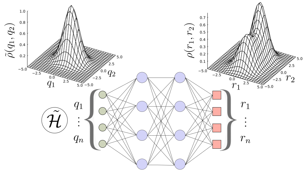
Fig. 1: Schematic representation of the SCHA on a neural network curved manifold. The Gaussian density matrix $\tilde{\rho}$, solution of the trial harmonic Hamiltonian $\tilde{\mathcal{H}}$ in an auxiliary space $\bm{q}$ (the curved manifold) is transformed into real space thanks to the transformation ${\bm{r}}(\bm{q})$ defined through a neural network. The nonlinearity of the transformation deforms the Gaussian shape and introduces new features on the final density matrix, including correlations beyond the original distribution.

We start briefly reviewing the SCHA in Sec. II, extending the theory in the case of indistinguishable particles, with particular care to the case of fermions (Sec. III). Then, we introduce the curved manifold that allows the wavefunction to deviate from the original Gaussian shape (Sec. IV). We discuss the neural network parametrization of the curved manifold (Sec. V) and how to encode crystal symmetries within it. Sec. VI discusses the specific requirements of the neural network parametrization to deal with fermionic degrees of freedom. In Sec. VII, we apply the new theory to study several challenging cases where the SCHA fails, such as the profound double-well potential (to model quantum tunneling), the hydrogen atom (to model the electron-ion cusp), and the H2 dissociation (to model electron-electron correlations), both in the ground bonding state (singlet) and in the excited antibonding one (triplet) (Sec. VII.4).

II Self-Consistent Harmonic Approximation

The self-consistent harmonic approximation is a variational approach to the solution of the time-independent Schrödinger equation:

$$\hat{H}\ket{\psi}=E\ket{\psi},$$ (1)

where $\ket{\psi}$ is the ground-state wave-function of a generic Hamiltonian operator $\hat{H}$, and $E$ is its associated energy. We indicate with a hat $\hat{\cdot}$ an operator in the Hilbert space. The SCHA was successfully employed to solve the nuclear quantum problem, where $\hat{H}$ depends only on atomic coordinates, and the electrons’ degrees of freedom are integrated out within the Born-Oppenheimer approximation. Here, we extend the formalism to electrons. Thus, $\hat{H}$ depends on the position operators $\hat{R}_{i}$ of both nuclei and electrons, overcoming the Born-Oppenheimer approximation. We neglect the role of spin interactions, such as spin-orbit coupling, and assume that the total spin operator $\hat{S^{2}}$ and its projection on one axis $\hat{S_{z}}$ commute with the Hamiltonian $\hat{H}$. The SCHA constrains the wavefunction $\ket{{\tilde{\psi}}}$ to the ground state of an auxiliary harmonic Hamiltonian ${\hat{\mathcal{H}}}[\bm{\mathcal{R}},\bm{\Phi}]$ depending on the parameters $\bm{\mathcal{R}}$ and $\bm{\Phi}$ as

$${\hat{\mathcal{H}}}[\bm{\mathcal{R}},\bm{\Phi}]=\hat{K}+\frac{1}{2}\sum_{ij}(\hat{R}_{i}-\mathcal{R}_{i})\Phi_{ij}(\hat{R}_{j}-\mathcal{R}_{h}),$$ (2)

$${\hat{\mathcal{H}}}[\bm{\mathcal{R}},\bm{\Phi}]\ket{{\tilde{\psi}}[\bm{\mathcal{R}},\bm{\Phi}]}={\mathcal{E}}\ket{{\tilde{\psi}}[\bm{\mathcal{R}},\bm{\Phi}]},$$ (3)

where $\hat{K}$ is the kinetic energy operator, $\hat{R}_{i}$ is the position operator of the $i$-th particle (electron or nucleus). Latin indices indicate both the particle and the Cartesian component, and bold symbols represent tensorial quantities (e.g., vectors and matrices). The vector $\mathcal{R}_{i}$ indicates the average position of particle $i$ (centroids), while $\bm{\Phi}$ are auxiliary force constant matrices encoding the quantum fluctuations and the correlations between different particles. These parameters must minimize the total energy within the Rayleigh-Ritz variational principle

$$E^{\text{(SCHA)}}=\min_{\bm{\mathcal{R}},\bm{\Phi}}\braket{{\tilde{\psi}}[\bm{\mathcal{R}},\bm{\Phi}]}{\hat{H}}{{\tilde{\psi}}[\bm{\mathcal{R}},\bm{\Phi}]}.$$ (4)

The minimum of Eq. (4) is satisfied by the self-consistent equationsSSCHA

$$\braket{{\tilde{\psi}}[\bm{\mathcal{R}},\bm{\Phi}]}{\frac{d\hat{V}}{dR_{i}}}{{\tilde{\psi}}[\bm{\mathcal{R}},\bm{\Phi}]}=0,$$ (5)

$$\braket{{\tilde{\psi}}[\bm{\mathcal{R}},\bm{\Phi}]}{\frac{d^{2}\hat{V}}{dR_{i}dR_{j}}}{{\tilde{\psi}}[\bm{\mathcal{R}},\bm{\Phi}]}=\Phi_{ij},$$ (6)

where $\hat{V}=V(\hat{\bm{R}})$ is the interaction potential as a function of the position operators of the particles. By solving Eq. (5) and Eq. (6) $\bm{\mathcal{R}}$ and $\bm{\Phi}$ are updated to get a new auxiliary Hamiltonian ${\hat{\mathcal{H}}}[\bm{\mathcal{R}}^{\text{(next)}},\bm{\Phi}^{\text{(next)}}]$, defining a ground state $\ket{{\tilde{\psi}}^{\text{(next)}}}$ for the next iteration. The process is repeated until convergence of Eq. (5) and Eq. (6).

The SCHA works at finite temperature by replacing the wavefunction with the density matrix $\hat{\rho}$ and the averages as traces. In this case, the auxiliary Hamiltonian defines the density matrix through the usual equilibrium relationship

$$\hat{\rho}[\bm{\mathcal{R}},\bm{\Phi}]=\frac{\exp\left(-\beta{\hat{\mathcal{H}}}[\bm{\mathcal{R}},\bm{\Phi}]\right)}{\mathcal{Z}},$$ (7)

$${\mathcal{Z}}=\textup{Tr}\left[\exp\left(-\beta{\hat{\mathcal{H}}}[\bm{\mathcal{R}},\bm{\Phi}]\right)\right].$$ (8)

We omit the explicit dependence of $\hat{\rho}$ from the $\bm{\mathcal{R}}$ and $\bm{\Phi}$ in the following equations. Indeed, the equilibrium solution is obtained by minimizing the free energy functional $\mathcal{F}[\hat{\rho}]$SSCHA

$$\mathcal{F}[\hat{\rho}]=\left\langle\hat{H}\right\rangle_{\hat{\rho}}-TS\left[\hat{\rho}\right],$$ (9)

where $T$ is the temperature and $S[\hat{\rho}]$ is the entropy functional, defined as

$$S[\hat{\rho}]=-k_{b}\left\langle\ln\hat{\rho}\right\rangle_{\hat{\rho}},$$ (10)

where the quantum averages are

$$\left\langle\hat{H}\right\rangle_{\hat{\rho}}=\textup{Tr}\left[\hat{\rho}\hat{H}\right],$$ (11)

and $k_{b}$ is the Boltzmann constant. The equilibrium free energy $F$ is always lower than the free energy functional $\mathcal{F}[\hat{\rho}]$ for any $\hat{\rho}$ that is not the exact equilibrium one. Thus, the self-consistent equations to update $\bm{\mathcal{R}}$ and $\bm{\Phi}$ are obtained by minimizing Eq. (9)

$$\left\langle\frac{dV}{dR_{i}}\right\rangle_{\hat{\rho}}=\textup{Tr}\left[\hat{\rho}\frac{dV}{dR_{i}}\right]=0,$$ (12)

$$\left\langle\frac{d^{2}V}{dR_{i}dR_{j}}\right\rangle_{\hat{\rho}}=\textup{Tr}\left[\hat{\rho}\frac{d^{2}V}{dR_{i}dR_{j}}\right]=\Phi_{ij}[\hat{\rho}].$$ (13)

III SCHA for electrons

In this section, we apply the SCHA to electrons, showing how it is possible to deal with a system of indistinguishable fermions within the SCHA framework. To describe a fermionic (or bosonic) system, the auxiliary harmonic Hamiltonian must commute with the operator $\bm{S}_{ij}$ that swaps the position of particle $i$ with $j$, for any $i$ and $j$. This imposes the constraints on $\bm{\mathcal{R}}$ and $\bm{\Phi}$

$$\forall i,j\qquad\bm{S}_{ij}\bm{\mathcal{R}}=\bm{\mathcal{R}},\qquad\bm{S}_{ij}\bm{\Phi}\bm{S}_{ij}^{\dagger}=\bm{\Phi}.$$ (14)

The result is that the centroid position must be the same for all electrons, reducing its independent components from $3N$ to $3$. The only surviving elements of the $\bm{\Phi}$ are the 6 independent degrees of freedom that encode the coupling between an electron with itself ($\bm{\Phi}^{\text{(same)}}$) and the 9 degrees of freedom that couple two different electrons ($\bm{\Phi}^{\text{(diff)}}$), for a total of 15 degrees of freedom (versus $3N(3N+1)/2$ for distinguishable particles)

$${\hat{\mathcal{H}}}=\hat{K} +\frac{1}{2}\sum_{i\alpha\beta}(\hat{R}_{i\alpha}-\mathcal{R}_{\alpha})\Phi^{\text{(same)}}_{\alpha\beta}(\hat{R}_{i\beta}-\mathcal{R}_{\beta})+$$

$$+\frac{1}{2}\sum_{\begin{subarray}{c}i\neq j\\ \alpha\beta\end{subarray}}(\hat{R}_{i\alpha}-\mathcal{R}_{\alpha})\Phi^{\text{(diff)}}_{\alpha\beta}(\hat{R}_{j\beta}-\mathcal{R}_{\beta}).$$ (15)

In this section, we explicitly encode with $i\alpha$ and $j\beta$ the index of the particle and the cartesian coordinate. While $\bm{\Phi}^{\text{(same)}}$ is hermitian, the same is not necessarily valid for $\bm{\Phi}^{\text{(diff)}}$. Notably, $\bm{\Phi}^{\text{(diff)}}$ is a coupling term between electrons. Therefore, the SCHA differs from other mean-field approaches like Hartree-Fock (HF) and density-functional theory (DFT) because the auxiliary Hamiltonian already accounts for a certain degree of electronic correlation. Eq. (15) can be diagonalized exactly, and the resulting eigenstates cannot be separated into products of independent particle wave functions. However, it is challenging to disentangle the bosonic-fermionic statistics of the states. Also, we prove in Appendix E that $\bm{\Phi}^{\text{(diff)}}\to 0$ in the $N\to\infty$ limit. For these reasons, we further restrict the problem to noninteracting fermions in a harmonic potential, neglecting the correlations in the harmonic Hamiltonian. We show in Sec. V that this correlation can be restored on the density matrix a posteriori with a linear deformation of the curved manifold.

Without $\bm{\Phi}^{\text{(diff)}}$, the Hamiltonian Eq. (15) is noninteracting, and it can be diagonalized by identifying the three eigenvectors of $\bm{\Phi}^{\text{(same)}}$. Introducing the standard creation $a_{\mu}^{\dagger}$ and annihilation $a_{\mu}$ operators of the harmonic oscillator along each of these three modes $\mu$, we have

$${\hat{\mathcal{H}}}=\frac{1}{2}\sum_{\mu=1}^{3}\omega_{\mu}\left(2a_{\mu}^{\dagger}a_{\mu}+1\right).$$ (16)

A 3-state vector $\ket{n_{1}n_{2}n_{3}}$ uniquely identifies the state, encoding the excited level on each polarization mode. The overall fermionic wavefunction is obtained by constructing a Slater determinant with these orbitals similar to standard mean-field approaches, constraining the rules for populating states given by the Pauli exclusion principle, as shown in Fig. 2.

Fig. 2: States of the noninteracting fermionic oscillator in 3D. Electrons populate the excited states of the harmonic Hamiltonian $\ket{n_{1}n_{2}n_{3}}$ according to the Fermi-Dirac statistics and the spin multiplicity.

Notably, the electronic oscillator’s ground state is a Gaussian only up to 2 electrons. Excited orbitals are occupied for more than two electrons, and the many-body ground state acquires the nodes typical of fermionic wavefunctions. In the variational frameworks of the SCHA, the nodes are not fixed and depend on the parameters $\bm{\mathcal{R}}$ e $\bm{\Phi}^{\text{(same)}}$. Thus, the electronic SCHA does not rely on any fixed-node approximation necessary for applying path-integral Monte Carlo or diffusion Monte Carlo to fermionsfoulkes_quantum_2001 .

IV SCHA in a curved manifold

While the SCHA has been shown to work exceptionally well in investigating the anharmonic quantum motion of nuclei in crystalsErrea2016_H3S ; Aseginolaza2019 ; verdi_quantum_2023 ; Romanin2021 ; ranalli_temperature-dependent_2023 ; Pedrielli2022 ; Monacelli2020_NatPhys ; Monacelli2023_hydro ; Errea2020_Nature , its limitations arise from constraining the density matrix to solve a harmonic Hamiltonian. In the case of distinguishable particles like atomic nuclei, the real-space expression $\rho(\bm{R},\bm{R}^{\prime})=\braket{\bm{R}^{\prime}}{\hat{\rho}}{\bm{R}}$ of the SCHA density matrix is a GaussianMonacelli2021 . A Gaussian distribution fits the fluctuations of nuclei vibrating in a solid lattice. Still, it fails to capture ionic diffusion, molecular rotations, quantum tunneling, or cases where the wave function extends beyond the interatomic distance. These cases are significant for electrons, where their lighter mass by at least 3 orders of magnitude causes a quantum delocalization across a broad region of space, often encompassing many atoms by forming chemical bonds.

Overcoming the SCHA has proven more difficult than expected: any attempt to augment the auxiliary harmonic Hamiltonian with extra anharmonic terms prevents the analytical solvability of the auxiliary system. This results in the loss of many of the technique’s advantages, among which is the analytical expression for the entropySSCHA , fundamental to computing the phase diagram of materials. An alternative strategy consists of maintaining the auxiliary Hamiltonian harmonic, introducing a nonlinear change of variables between the Cartesian positions $\bm{R}$ and the degrees of freedom of the auxiliary Hamiltonian $\bm{q}$siciliano_beyond_2024 ; siciliano_beyond_2024-1 . This defines the auxiliary harmonic Hamiltonian on a manifold whose curvature is parametrized by the invertible transformation $\bm{R}(\bm{q})$. The expression of physical observables must be the same on the curved manifold $\bm{q}$ and real space $\bm{R}$.

$$\left\langle\hat{O}\right\rangle_{\hat{\rho}}=\textup{Tr}\left[\hat{\tilde{\rho}}\hat{O}\right]$$ (17)

$$\left\langle\hat{O}\right\rangle_{\hat{\rho}}=\int d\bm{R}d\bm{R}^{\prime}O(\bm{R},\bm{R}^{\prime})\rho(\bm{R}^{\prime},\bm{R}),$$ (18)

$$\left\langle\hat{O}\right\rangle_{\hat{\rho}}=\int d\bm{q}d\bm{q}^{\prime}\tilde{O}(\bm{q},\bm{q}^{\prime})\tilde{\rho}(\bm{q}^{\prime},\bm{q}),$$ (19)

where we indicated with a tilde $\tilde{\cdot}$ quantities evaluated on the curved manifold. By imposing that the density matrix conserves the probability density in the position space, we can prove that diagonal observables like $O(\bm{R},\bm{R}^{\prime})\propto\delta(\bm{R}-\bm{R}^{\prime})$ transform like

$$\tilde{O}(\hat{\bm{q}})=O(\bm{R}(\hat{\bm{q}})),$$ (20)

and the density matrix as

$$\tilde{\rho}(\bm{q},\bm{q}^{\prime})=\rho(\bm{R}(\bm{q}),\bm{R}(\bm{q}^{\prime}))\sqrt{\det\bm{{\mathcal{J}}}(\bm{R}(\bm{q}))\det\bm{{\mathcal{J}}}(\bm{R}(\bm{q}^{\prime}))},$$ (21)

where $\bm{{\mathcal{J}}}$ is the jacobian of the transformation

$${\mathcal{J}}_{ab}(\bm{q})=\frac{\partial R_{a}}{\partial q_{b}}.$$ (22)

The transformation of Eq. (21) preserves the probability density in the position space. A more complex transformation for the observable needs to be derived if $O(\bm{R},\bm{R}^{\prime})$ is not diagonal in the position basis, e.g., for the kinetic energy.

We have, thus, two different density matrices: $\tilde{\rho}(\bm{q},\bm{q}^{\prime})$, defined on the curved manifold and solution of the auxiliary harmonic Hamiltonian (Eq. 8), and $\rho(\bm{R},\bm{R}^{\prime})$, the transformed density matrix in Cartesian space. Notably, $\rho(\bm{R},\bm{R}^{\prime})$ is the real density matrix of our solution, which depends on the parameters that define the auxiliary Hamiltonian ($\bm{\mathcal{R}}$ and $\bm{\Phi}$) and on the curvature of the manifold, defined by the metric tensor $g_{ab}$ as

$$g_{ab}(\bm{q})=\sum_{c}\frac{\partial R_{c}}{\partial q_{a}}\frac{\partial R_{c}}{\partial q_{b}}=\sum_{c}{\mathcal{J}}_{ca}{\mathcal{J}}_{cb},$$ (23)

$$\sqrt{\det{\bm{g}}}=\sqrt{\det\bm{{\mathcal{J}}}(\bm{R}(\bm{q}))\det\bm{{\mathcal{J}}}(\bm{R}(\bm{q}^{\prime}))}.$$ (24)

This allows us to increase the degrees of freedom of the ansatz density matrix thanks to the metric tensor $\bm{g}$ while keeping the auxiliary system harmonic. This approach maintains all the advantages of the original SCHA. In fact, all observables can be evaluated in the curved manifold, where the density matrix is harmonic.

IV.1 Free energy in the curved manifold

The target of the SCHA as a variational theory is to optimize the trial density matrix $\rho(\bm{R},\bm{R}^{\prime})$ to minimize the free energy. The free energy $F[\hat{\rho}]$ is a functional of the density matrix comprising the internal energy $U[\hat{\rho}]=\left\langle\hat{H}\right\rangle_{\hat{\rho}}$ and the entropy $S[\hat{\rho}]$. The most complex part of the free energy is the entropy, for which the expression is challenging to be converged numerically

$$S[\hat{\rho}]=-k_{b}\braket{\ln\hat{\rho}}.$$ (25)

In fact, due to the logarithm, even very high energy states are important in the average of Eq. (25), and it cannot be computed as an average on the sampled configurations. However, if the nonlinear transformation $\bm{R}(\bm{q})$ is bijective on $\mathbb{R}^{3N}\to\mathbb{R}^{3N}$, the entropy of $\rho(\bm{R},\bm{R}^{\prime})$ coincides with the one of $\tilde{\rho}(\bm{q},\bm{q}^{\prime})$siciliano_beyond_2024 . Thus, $S[\hat{\rho}]$ can be evaluated conveniently on the curved manifold, where the density matrix solves the auxiliary harmonic Hamiltonian ${\hat{\mathcal{H}}}[\bm{\mathcal{R}},\bm{\Phi}]$ for which the energy levels are known analytically. In the case of distinguishable particles, like atomic nuclei, the entropy has a simple expression depending on the frequencies $\omega_{\mu}$ of the auxiliary Hamiltonian

$$\sum_{b}\frac{\Phi_{ab}}{\sqrt{m_{a}m_{b}}}e_{\mu}^{a}=\omega_{\mu}^{2}e_{\mu}^{b},$$ (26)

$$S[\rho(\bm{R},\bm{R}^{\prime})]=\frac{k_{b}}{2}\sum_{\mu}\left[\frac{\beta\hbar\omega_{\mu}}{\tanh\frac{\beta\hbar\omega_{\mu}}{2}}-2\log\left(\sinh\frac{\beta\hbar\omega_{\mu}}{2}\right)\right],$$ (27)

where $m_{a}$ is the mass of the $a$ particle, $\beta=(k_{b}T)^{-1}$ is the Boltzmann factor. In the more general case of mixtures between distinguishable and indistinguishable particles, the energy levels of the auxiliary harmonic Hamiltonian must be appropriately populated, accounting for the specific Fermi-Dirac or Bose-Einstein statistic and the particles’ spin. Thankfully, the auxiliary harmonic Hamiltonian can be decoupled between each different kind of particle, separating the indistinguishable fermions (electrons) and the distinguishable ions. The electronic entropy is thus evaluated in a noninteracting harmonic system, as discussed in Sec. III. Let $f_{i}$ be the occupation number of the $i$ state of the auxiliary harmonic Hamiltonian, the resulting electronic entropy is

$$S[\hat{\rho}]=-k_{b}\sum_{i}\left[f_{i}\ln(f_{i})+(1-f_{i})\ln(1-f_{i})\right].$$ (28)

The internal energy $U[\hat{\rho}]$ accounts for kinetic and potential energy. The potential energy is a diagonal operator in the position of the particles $\hat{R}$, and can be evaluated on the curved manifold following Eq. (20)

$$\left\langle\hat{V}\right\rangle_{\hat{\rho}}=\int d\bm{q}\;V\left(\bm{R}(\bm{q})\right)\tilde{\rho}(\bm{q}).$$ (29)

Eq. (29) is the average interacting potential in the curved manifold. The practical computation of $\left\langle\hat{V}\right\rangle_{\hat{\rho}}$ through Monte Carlo consists of generating a random ensemble of particles on the positions $\bm{q}$ in the manifold exploiting the Gaussian shape of the auxiliary probability distribution given by $\tilde{\rho}(\bm{q})$, transforming the coordinates from the manifold $\bm{q}$ to Cartesian space $\bm{R}$ with the transformation $\bm{R}(\bm{q})$, and averaging the values of the potential $V(\bm{R})$ in Cartesian space. Compared with other approaches like PIMD or QMC, the generation of the ensemble is faster and does not require any Metropolis algorithm or thermalization process, as it occurs on a Gaussian distribution in the curved manifold.

The kinetic energy is more complex as it is nondiagonal in position space. Its expression $\tilde{K}(\bm{q},\bm{q}^{\prime})$ on the curved manifold is derived by transforming the integration variables from Cartesian space

$$\left\langle K\right\rangle_{\hat{\rho}}=-\sum_{i}\frac{\hbar^{2}}{2m_{i}}\int d\bm{R}d\bm{R}^{\prime}\delta(\bm{R}-\bm{R}^{\prime})\frac{\partial^{2}}{\partial R^{\prime}_{i}}\rho(\bm{R},\bm{R}^{\prime})$$ (30)

$$\left\langle K\right\rangle_{\hat{\rho}}=\int d\bm{q}d\bm{q}^{\prime}\tilde{K}(\bm{q},\bm{q}^{\prime})\tilde{\rho}(\bm{q},\bm{q}^{\prime})$$ (31)

In Appendix A we derive the explicit expression of $\tilde{K}(\bm{q},\bm{q}^{\prime})$, which is

$$\tilde{K}(\bm{q}, \bm{q}^{\prime})=-\sum_{i}\frac{\hbar^{2}}{2m_{i}}\delta(\bm{q}-\bm{q}^{\prime})\cdot$$

$$\left[\alpha^{i}(\bm{q})+\sum_{a}\beta_{a}^{i}(\bm{q})\frac{\partial}{\partial q_{a}^{\prime}}+\sum_{ab}\gamma^{i}_{ab}(\bm{q})\frac{\partial^{2}}{\partial q^{\prime}_{a}\partial q^{\prime}_{b}}\right].$$ (32)

Here, $\bm{\alpha}(\bm{q})$, $\bm{\beta}(\bm{q})$ and $\bm{\gamma}(\bm{q})$ are operators that depend on the local curvature of the manifold. Their explicit expression is reported in Appendix A. Indeed, in the case of a flat manifold, we recover $\bm{\alpha}=\bm{\beta}=0$, $\gamma^{i}_{ab}(\bm{q})=\delta_{ab}$ and $\tilde{K}(\bm{q},\bm{q}^{\prime})$ matches the definition of the kinetic energy on a flat space (Eq. 30). Interestingly, the kinetic energy comprises a diagonal operator in the positions resembling a potential energy term, the $\bm{\alpha}(\bm{q})$, similar to the correlation potential defined within DFT. The second term, $\bm{\beta}(\bm{q})$, mixes momentum and position operators, generating a similar effect to a magnetic field. The last term is the classical kinetic energy transformed, where the position dependency of the $\gamma_{ab}^{i}(\bm{q})$, as well as the mixed second derivative, can be interpreted as the mass of particles acquiring a dependency on the space due to the curvature (more details in Appendix F). Notably, Eq. (31) differs from the equation presented in Ref.siciliano_beyond_2024 , as here we do not perform any hypothesis on the Gaussian shape of the auxiliary density matrix $\tilde{\rho}(\bm{q},\bm{q}^{\prime})$. This way, Eq. (31) can also be applied to electrons, excited states, or any nonharmonic auxiliary Hamiltonian.

V Neural network parametrization of the curved manifold

In Sec. IV.1, we derived the free energy expression on the curved manifold, where the density matrix is the ground state of an auxiliary harmonic Hamiltonian, and the free energy can be computed efficiently. To solve the quantum problem beyond the SCHA, we need to minimize the free energy by optimizing the parameters defining the auxiliary Hamiltonian and the manifold. The auxiliary Hamiltonian depends on the centroids $\bm{\mathcal{R}}$ and the effective force constants $\bm{\Phi}$. Ref. siciliano_beyond_2024-1 devised a specific manifold from a cartographic representation of spherical coordinates to describe molecular rotations. While it provides an excellent solution to enhance the SCHA by enabling molecules to rotate thanks to the manifold’s curvature, it is too restrictive to capture the complex features of the electronic wavefunction. Here, we introduce a general transformation that can be systematically improved to parameterize any possible curved manifold, thus significantly enhancing the variational space of density matrices.

The manifold is defined through the transformation $\bm{R}(\bm{q})$. This function maps $\mathbb{R}^{N}\to\mathbb{R}^{N}$, is bijective, continuous, and differentiable. We define the Gaussian stretchers as the class of manifolds parametrized by the transformation

$$\bm{R}(\bm{q})=\bm{{\mathcal{Q}}}+\tilde{\bm{q}}\left[1+(e^{\zeta}-1)\exp\left(-\frac{1}{2}\sum_{cd}\tilde{q}_{c}\Gamma_{cd}\tilde{q}_{d}\right)\right],$$ (33)

where

$$\tilde{\bm{q}}=\bm{q}-\bm{{\mathcal{Q}}},$$ (34)

and $\bm{\Gamma}$ is positive definite. As the name suggests, this transformation stretches the space, deforming the density matrix in the position identified by $\bm{{\mathcal{Q}}}$ along the principal axis of the $\bm{\Gamma}^{-1}$ covariance matrix, with intensity $\zeta$. Outside the central position $\bm{{\mathcal{Q}}}$ and the range of the covariance matrix $\bm{\Gamma}^{-1}$, the exponential of Eq. (33) becomes small and the manifold flat ($\bm{R}=\bm{q}$). Therefore, the Gaussian stretcher only warps the space inside the Gaussian by stretching the density matrix with a positive curvature if $\zeta>0$ (reducing the probability distribution at the center and accumulating it on the edges) or compressing it with a negative curvature if $\zeta<0$ (reducing the probability on the edges to accumulate it on the center). The parameterization of the Gaussian stretcher is only valid for $\zeta<\zeta_{c}\approx 1.1$, above which the transformation defined in Eq. (33) is no longer bijective.

Each Gaussian stretcher has the same number of degrees of freedom as the original SCHA algorithm plus $\zeta$ (the $\bm{\Gamma}$ symmetric 2-rank tensor is equivalent to the auxiliary force constant matrix $\bm{\Phi}$, and the $\bm{{\mathcal{Q}}}$ vector has the same length as the centroids $\bm{\mathcal{R}}$). Moreover, multiple Gaussian stretchers can be stacked together in layers as in neural networks:

$$\bm{q}_{n+1}=\bm{{\mathcal{Q}}}_{n}+\tilde{\bm{q}}_{n}\left[1+(e^{\zeta_{n}}-1)\exp\left(-\frac{1}{2}\sum_{cd}\tilde{q_{n}}_{c}\Gamma^{(n)}_{cd}\tilde{q_{n}}_{d}\right)\right],$$ (35)

$$\bm{q}_{0}=\bm{R}\qquad\bm{{\mathcal{Q}}}_{0}=\bm{\mathcal{R}}.$$ (36)

Each new layer introduces three new parameters: $\zeta_{n}$, $\bm{{\mathcal{Q}}}_{n}$, and $\bm{\Gamma}^{(n)}$. In the case of concatenated Gaussian stretchers, the resulting manifold exhibits a complex curvature that is fine-tuned in any position by a layer with a nearby centroid $\bm{{\mathcal{Q}}}_{n}$. The transformation resembles a neural network where the activation function for each neuron is given by Eq. (33). In Appendix C, we evaluate the metric tensor and the expression of the kinetic energy $\tilde{K}(\bm{q},\bm{q}^{\prime})$ defined in Eq. (32). The manifold parameters are optimized through a standard ADAM algorithmADAM , where the gradient of the quantum free energy is evaluated with back-propagation, a technique commonly employed in neural networks.

Equivariance under specific symmetries can be enforced on the Gaussian stretcher manifold. This is pivotal for ensuring compliance with fundamental laws of physics, like the acoustic sum rule (equivariance with respect to global translations) and the permutation of indistinguishable particles. Moreover, this characteristic extends to any symmetry operation commuting with the original Hamiltonian as the crystallographic symmetry group. In particular, let $\bm{S}$ be the symmetry operator; the manifold is equivariant under $\bm{S}$ if

$$\bm{R}(\bm{S}\bm{q})=\bm{S}\bm{R}(\bm{q}).$$ (37)

This condition can be applied layer by layer on the Gaussian stretcher as

$$\bm{S}\bm{q}_{n+1}=\bm{{\mathcal{Q}}}_{n}+(\bm{S}\bm{q}_{n}-\bm{{\mathcal{Q}}}_{n})f_{n}(\bm{S}\bm{q}_{n}),$$ (38)

where

$$f_{n}(\bm{q})=1+\left(e^{\zeta_{n}}-1\right)\exp\left[-\frac{1}{2}(\bm{q}-\bm{{\mathcal{Q}}}_{n})\bm{\Gamma}^{(n)}(\bm{q}-\bm{{\mathcal{Q}}}_{n})\right],$$ (39)

resulting in the following conditions that restrict the degrees of freedom of $\bm{{\mathcal{Q}}}_{n}$ and $\bm{\Gamma}^{(n)}$

$$\bm{S}\bm{{\mathcal{Q}}}_{n}=\bm{{\mathcal{Q}}}_{n},\qquad f_{n}(\bm{q})=f_{n}(\bm{S}\bm{q}).$$ (40)

The constraint on $\bm{{\mathcal{Q}}}_{n}$ enforces the centroid of the network to be a high-symmetry point of the crystal (Wyckoff position), while the constraint on $f_{n}$ enforces the symmetry on the $\bm{\Gamma}$ matrix as

$${\bm{S}}{}^{\dagger}\bm{\Gamma}_{n}\bm{S}=\bm{\Gamma}_{n}.$$ (41)

These conditions coincide with the ones complied by $\bm{\mathcal{R}}$ and $\bm{\Phi}$ in the standard harmonic Hamiltonian to preserve the symmetry of the density matrix. Therefore, imposing symmetries on the Gaussian stretchers is equivalent to constraining symmetries of positions and dynamical matrices.

Imposing crystal symmetries by constraining each layer of the nonlinear transformation suppresses the size of the variational space spanned by the Gaussian stretchers. Therefore, we resort to this scheme only for symmetries that preserve the physical meaning of the resulting density matrix, like the exchange between indistinguishable particles and the total translational symmetry. Any further symmetry constraint is imposed a posteriori throughout a Lagrange multiplier like

$$\mathcal{L}=\sum_{i=1}^{N}\left\|\bm{S}\bm{q}^{(n)}(\bm{q}^{(1)}_{i})-\bm{q}^{(n)}(\bm{S}\bm{q}^{(1)}_{i})\right\|^{2}.$$ (42)

By including $\mathcal{L}$ in the cost function to minimize the free energy, symmetries can be imposed a posteriori only between the first and the last layer of the Gaussia stretcher, thus increasing the variational degrees of freedom of the solution.

Since multiple transformations can be stacked layer-by-layer, it is also convenient to employ a linear transformation. In normal circumstances, this is redundant with the SCHA itself. the SCHA centroids $\bm{\mathcal{R}}$ and auxiliary force constant matrix $\bm{\Phi}$ act as a linear transformation on an uncorrelated ensemble of normalized Gaussians. The transformation reads as

$$\bm{q}^{(1)}=\bm{\mathcal{R}}+\bm{L}\bm{q}^{(0)},$$ (43)

$$\bm{L}\bm{L}^{\dagger}=\bm{\Upsilon}^{-1},$$ (44)

where $\bm{\Upsilon}^{-1}$ is the covariance matrix of the SCHA distribution

$$\Upsilon_{ab}=\sqrt{m_{a}m_{b}}\sum_{\mu}\frac{2\omega_{\mu}}{2n_{\mu}+1}e_{\mu}^{a}e_{\mu}^{b}.$$ (45)

Using a first (or last) linear layer is a feature familiar to standard machine learning neural networks. Besides the resemblance with machine learning, using the linear transformation matrix $\bm{L}$ as a variational degree of freedom instead of the auxiliary force constant matrix $\bm{\Phi}$ ensures the continuity of the transformation of the ensemble even in the presence of mode crossing and degeneracies if the original ensemble $q^{(0)}$ is kept fixed. This is essential to have a smooth and differentiable energy landscape (cost function). Moreover, in the case of indistinguishable particles, this linear transformation can restore the harmonic correlation lost by considering $\bm{\Phi}^{\text{(diff)}}\to 0$ in Eq. (15) to simplify the population of fermionic degrees of freedom. Without loss of generality, $\bm{L}$ can be written as

$$L_{ab}=\frac{1}{\sqrt{m}_{a}}\sum_{\mu}\sqrt{\frac{2\omega_{\mu}}{2n_{\mu}+1}}e_{\mu}^{a}e_{\mu}^{b},$$ (46)

thus satisfying Eq. (44).

VI Fermionic states

In this section, we present the constraints that the Gaussian stretcher have to satisfy to preserve the fermionic (or bosonic) character of the auxiliary density matrix $\tilde{\rho}(\bm{q},\bm{q}^{\prime})$ when it is transformed into the real space density matrix $\hat{\rho}(\bm{R},\bm{R}^{\prime})$. This is the fundamental requirement to treat indistinguishable particles within the formalism presented in this work. In Sec. III, we introduced the noninteracting fermionic wavefunction solving the auxiliary harmonic Hamiltonian. The manifold curvature mixes the degrees of freedom of different particles, leading to a correlated state. To preserve the antisymmetric characteristic of the underlying density matrix across the nonlinear transformation $\bm{R}(\bm{q})$, the manifold should preserve the exchange operation between different particles. It is trivial to show that $\rho(\bm{R},\bm{R}^{\prime})$ is a antisymmetric if $\tilde{\rho}(\bm{q},\bm{q}^{\prime})$ is antisymmetric and $\bm{R}(q)$ satisfies the condition

$${\bm{R}}_{1}(\bm{q}_{1},\bm{q}_{2},\cdots)={\bm{R}}_{2}(\bm{q}_{2},\bm{q}_{1},\cdots),$$ (47)

where with $\bm{q}_{1}$ (and $\bm{R}_{1}$) we indicate the components of $\bm{q}$ (and $\bm{R}$) on particle $1$, $1$ and $2$ are any two fermions, and the $\cdots$ indicates that the $\bm{q}$ vectors of the other particles have not been exchanged. Eq. (47) is fulfilled by a transformation of the kind:

$$\bm{R}(\bm{q})=\left\{\begin{array}[]{l}\displaystyle\bm{R}_{1}(\bm{q})=f(\bm{q})\bm{q}_{1}\\ \\ \displaystyle\bm{R}_{2}(\bm{q})=f(\bm{q})\bm{q}_{2}\\ \\ \qquad\;\;\,\vdots\end{array}\right.$$ (48)

where $f(\bm{q})$ is a generic symmetric function with respect to particle changes. The Gaussian stretchers meet this condition if ${\mathcal{Q}}$ is the same for all electrons and most of $\bm{\Gamma}$ parameters are constrained so that

$${\mathcal{Q}}_{(i,\alpha)}={\mathcal{Q}}_{(j,\alpha)},$$ (49)

$$\Gamma_{(i,\alpha)(i,\beta)}=\Gamma_{(j,\alpha)(j,\beta)},$$ (50)

$$\Gamma_{(i,\alpha)(j,\beta)}=\Gamma_{(j,\alpha)(k,\beta)},$$ (51)

where the index $(i,\alpha)$ indicates atom $i$ and Cartesian coordinate $\alpha$, for any choice of the atoms $i,j,k$. These are the same conditions as the $\bm{\mathcal{R}}$ and $\bm{\Phi}$ matrix of the auxiliary harmonic Hamiltonian for fermions we derived in Sec. III. Thanks to the cross diagonal terms of $\bm{\Gamma}$ (Eq. 51), the transformation can still couple different particles, introducing correlations at each layer of the nonlinear transformation defining the curved manifold. Another consequence of the exchange symmetry of the manifold is the combinatorial number of constraints imposed on the degrees of freedom that counterbalance their growth when the number of particles increases: above two electrons, the degrees of freedom do not increase with the number of particles on each layer of the Gaussian stretcher.

VII Applications and examples

In this section, we illustrate some applications to show how the Gaussian stretcher manifold systematically improves the SCHA result. We start with a one-particle problem, where deviations from the Gaussian ground state are significant, like in the case of a profound double-well potential in Sec. VII.1, a Coulomb potential (hydrogen atom) in Sec. VII.3, and finally for interacting electrons in the dissociation of the H2 molecule (Sec. VII.4). We discuss and display also the capabilities of the method to capture excited states by exciting electrons in the auxiliary harmonic Hamiltonian for the 1D double potential and the H2 dissociation in the antibonding triplet electronic configuration.

VII.1 Double well potential

The double well potential is a classic example of a strongly anharmonic system. It is also a good prototype for testing quantum tunneling, a regime in which the SCHA is known to fail. We represent the double well potential of a 1D particle as

$$V(R)=aR^{4}-bR^{2}.$$ (52)

For values of $b>0$, the harmonic approximation presents an imaginary frequency in $R=0$, and the system becomes highly anharmonic. Here, we compare the performances of the standard SCHA and the SCHA in the multi-layer Gaussian stretcher manifold introduced in this work against the exact (numerical) solution.

The double well potential has three regimes as $b$ varies. When $b^{3}\gg\frac{2a^{2}}{m^{2}}$ (in Hartree atomic units), the two wells are far apart, the energy barrier is too high, and the solution localizes into one of the minima (broken symmetry solution). The standard SCHA describes this regime well as the system becomes locally harmonic. The opposite occurs when the barrier is small ($b^{3}\ll\frac{2a^{2}}{m^{2}}$); in this case, quantum/thermal fluctuations entirely overcome the energy barrier, and the probability density is located in the saddle point $R=0$. This phase is also well captured by the standard SCHA. However, when the energy barrier is comparable with the quantum/thermal fluctuations ($b^{3}\approx\frac{2a^{2}}{m^{2}}$), tunneling or thermal hopping between the two minima occur on the same timescale as the lattice vibrations. This is the regime where we expect the SCHA to fail. Fig. 3(a) reports the error on the ground state energy versus the exact diagonalization of the potential in Eq. (52) as a function of the $b$ parameter (anharmonicity), comparing the standard SCHA and the generalized SCHA on a single-layer Gaussian stretcher manifold.

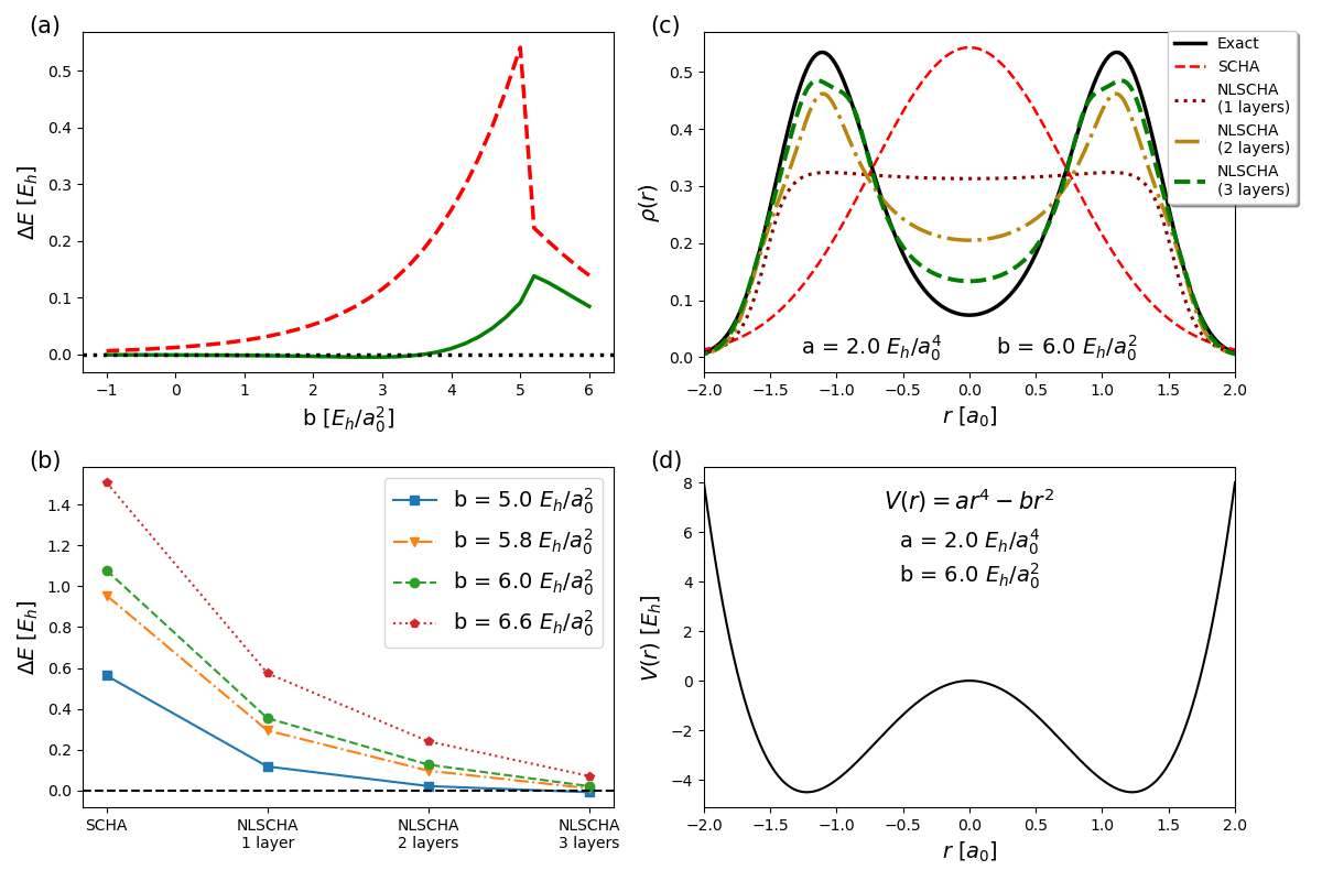
Fig. 3: Comparison between the SCHA, SCHA on the Gaussian stretcher manifold (here nonlinear SCHA, or NLSCHA), and exact (numerical) solution for a double well potential. (a) Error on the ground state energy of the potential Eq. (52) as a function of the $b$ parameter (anharmonicity). For $b>\sqrt[3]{\frac{2a^{2}}{m^{2}}}=$2\text{\,}\mathrm{\text{ $E_{\textup{ h }}$ }}\mathrm{/}\mathrm{\text{ $a_{0}$ }}^{2}$$, the system enters the quantum tunneling regime, where the zero-point energy of the wave function is below the barrier dividing the two minima of the potential. (b) The energy error at several values of $b$ and varying the number of layers. All the values are in the deep quantum regime $b>$2\text{\,}\mathrm{\text{ $E_{\textup{ h }}$ }}\mathrm{/}\mathrm{\text{ $a_{0}$ }}^{2}$$. The wavefunction is constrained to keep the inversion symmetry (inhibiting the transition into the localized state). (c) Modulus squared of the ground state wavefunction at $b=$6.0\text{\,}\mathrm{\text{ $E_{\textup{ h }}$ }}\mathrm{/}\mathrm{\text{ $a_{0}$ }}^{2}$$ by varying the number of layers of the nonlinear transformation (d) Potential energy landscape of the double well. The exact result has been evaluated numerically with the implicitly restarted Lanczos algorithmLanczos as implemented in Scipyscipy .

The improvement provided by the curved manifold is excellent, even with a single layer. As noted analytically, with $a=$2\text{\,}\mathrm{\text{ $E_{\textup{ h }}$ }}\mathrm{/}\mathrm{\text{ $a_{0}$ }}^{4}$$, the values for which we expect the SCHA failing are $b\geq\sqrt[3]{\frac{2a^{2}}{m^{2}}}=$2\text{\,}\mathrm{\text{ $E_{\textup{ h }}$ }}\mathrm{/}\mathrm{\text{ $a_{0}$ }}^{2}$$, which are well displayed in Fig. 3(a). Above $b=$2\text{\,}\mathrm{\text{ $E_{\textup{ h }}$ }}\mathrm{/}\mathrm{\text{ $a_{0}$ }}^{2}$$, the system enters the quantum tunneling regime, where the barrier is slightly above the zero-point energy, but the wavefunction manages to trespass the saddle point. The error of the SCHA quickly increases in this regime until $b\approx$5\text{\,}\mathrm{\text{ $E_{\textup{ h }}$ }}\mathrm{/}\mathrm{\text{ $a_{0}$ }}^{2}$$, where the system collapses in the broken symmetry solution around one of the two minima. From there, further increasing $b$ leads to a progressive suppression of the tunneling and, therefore, the improvement of the SCHA solution. The sudden collapse of the SCHA triggers a first-order-like phase transition, which is completely absent in the exact solution, as the system smoothly transits between these regimes without any divergence or discontinuity. When we employ a single layer Gaussian stretcher curved manifold, indicated as non-linear SCHA (NLSCHA), the solution preserves an excellent agreement with the exact result up to $b=$4\text{\,}\mathrm{\text{ $E_{\textup{ h }}$ }}\mathrm{/}\mathrm{\text{ $a_{0}$ }}^{2}$$, well within the tunneling regime. Also, NLSCHA suppresses the strong discontinuity observed within the SCHA between the tunneling and broken symmetry solution, even if a corner point is still evident in the energy.

Applying multiple layers of the Gaussian stretcher further reduces the error. In Fig. 3(b), we show the error as a function of the number of layers. Here, we constrain the inversion symmetry and prevent the solution from falling into the broken symmetry phase.

We report the comparison of the wave-function modulus with the exact solution in Fig. 3(c) in the deep tunneling regime, where the wavefunction is almost completely localized across the minima ($b=$6\text{\,}\mathrm{\text{ $E_{\textup{ h }}$ }}\mathrm{/}\mathrm{\text{ $a_{0}$ }}^{2}$)$. One layer of Gaussian stretcher is not enough to split the wavefunction in the two peaks around the minima of the potential, as it is energetically more convenient to reproduce the distribution’s tails due to the fast rise of the quartic potential. However, adding extra layers enables the separation of the peaks. As with SCHA, NLSCHA is a method that does not target reproducing the correct wave function but rather the total energy. The slight deviation between the exact wavefunction and the NLSCHA with three layers translates into total energy (and the thermodynamic properties) that depends quadratically on it.

The NLSCHA’s capability to reproduce the splitting between the wavefunction peaks and minimize the error in the non-broken symmetry solution has essential repercussions in the simulation of quantum tunneling, which was previously impossible within the standard SCHA or other harmonic-based approaches.

VII.2 Excited states

The new formalism introduced in this work also allows populating excited states in the auxiliary harmonic Hamiltonian, enabling the simulation of wavefunctions with nodes to optimize the total energy. This approach has already been successfully employed in VMC to study optical gaps in solid state systemsCuzzocrea2020 ; Dash2019 , and transfers naturally to SCHA. As a simple benchmark, we apply the NLSCHA to unveil the wavefunction of the first excited state of the double well potential in the strongly anharmonic regime. The comparison with the exact diagonalization is reported in Fig. 4.

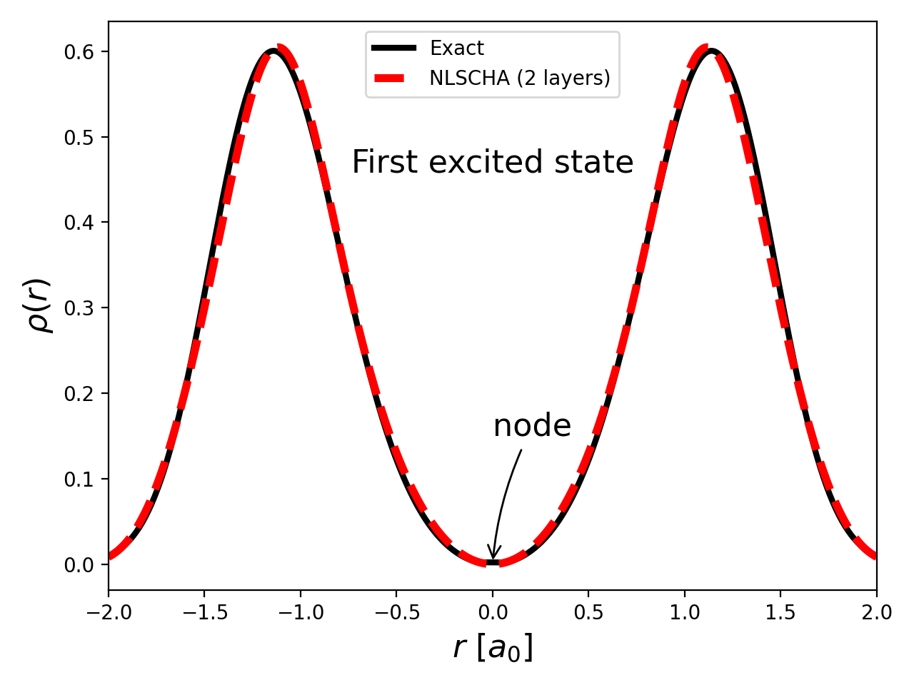
Fig. 4: Comparison between the exact and NeuroSCHA (2 layers) excited state density. The potential is a double well of the form $V(r)=ar^{4}-br^{2}$, where $a=$2\text{\,}\mathrm{\text{ $E_{\textup{ h }}$ }}\mathrm{/}\mathrm{\text{ $a_{0}$ }}^{4}$$ and $b=$-6\text{\,}\mathrm{\text{ $E_{\textup{ h }}$ }}\mathrm{/}\mathrm{\text{ $a_{0}$ }}^{2}$$, as in Fig. 3(c). We highlight the position of the node of the wavefunction in the origin.

The wavefunction agrees exceptionally well with the exact result already with just two layers of Gaussian stretcher manifold, outmatching even the precision in the ground state thanks to the presence of a node in the original wavefunction.

VII.3 Hydrogen atom

While the SCHA on a multilayer Gaussian stretcher manifold performs exceptionally well on ionic systems and solves many issues of the standard SCHA, like molecular rotations, delocalization, and tunneling, its applicability in the electronic problem has to be proven. Electronic correlated wavefunctions are strongly non-Gaussian, with cusps in the overlap between different electrons and electron-ion due to the divergence of the Coulomb potentialkato1957eigenfunctions . While some of the problems could be accounted for with the use of pseudo-potential like done in mean-field approaches with plane-wave basis set, in this section, we benchmark the expressibility of the transformed wavefunction on the hydrogen atom, a prototypical system with an electron-ion cusp that is highly challenging to all methods that do not explicitly account for the cusp in the wave-function (as it occurs in plane-wave codes).

We constrain the wavefunction for the hydrogen atom potential with a fully rotational symmetry group centered around the origin and the potential $V(r)=-1/r$, as discussed in Sec. V. We solve the system by progressively increasing the number of layers of the Gaussian stretchers. Thanks to the spherical symmetry constraints, each layer has only 2 degrees of freedom ($\zeta$ is free, $\Gamma$ is proportional to the identity matrix, and $\bm{{\mathcal{Q}}}=0$). The final wave functions and energies are reported in Fig. 5. Already with one layer, the long-range behavior of the wavefunction is very good ($r>$0.5\text{\,}\mathrm{\text{ $a_{0}$ }}$$), while increasing the number of layers further improves the $r\to 0$ limit (the cusp).

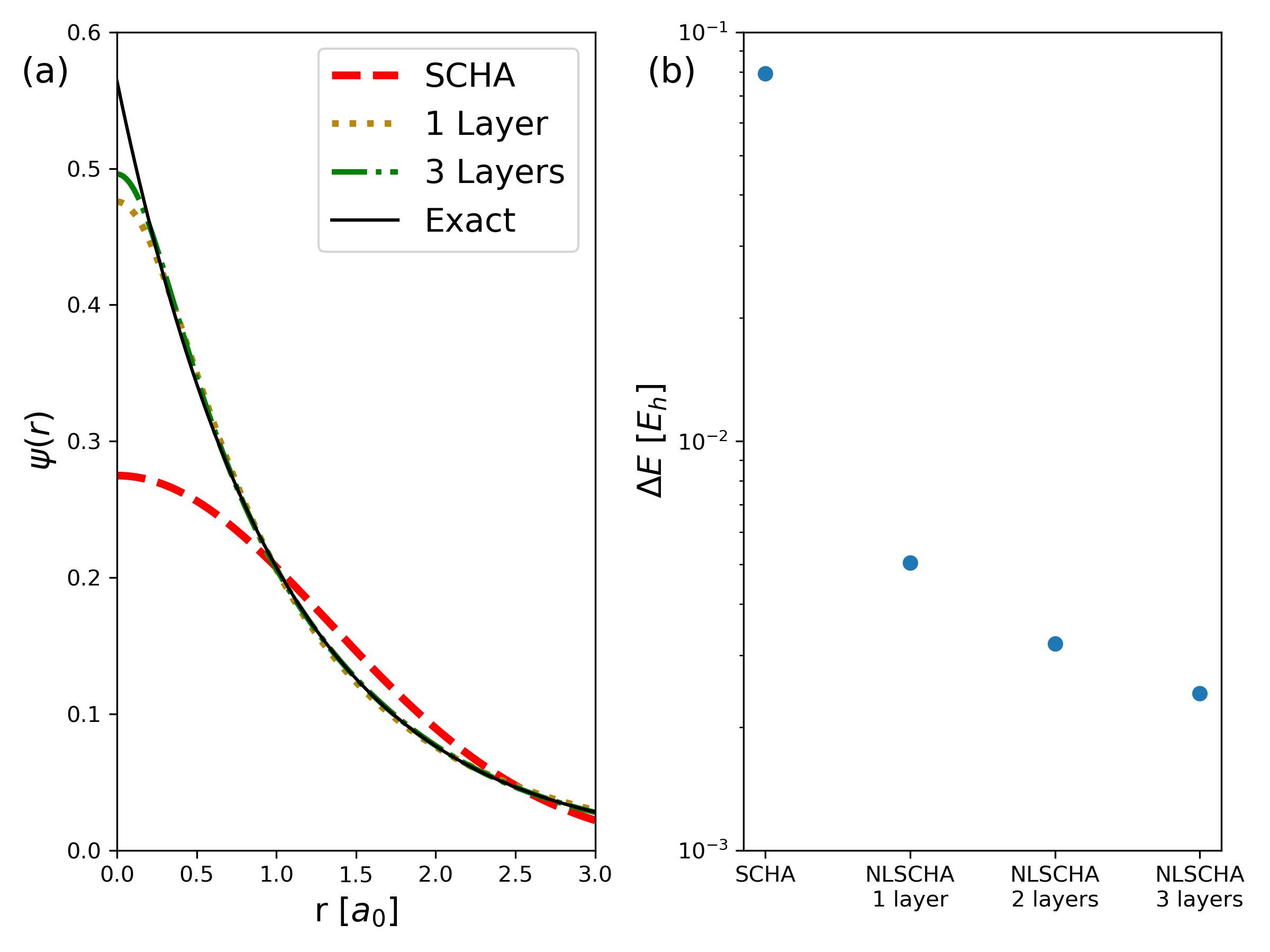
Fig. 5: Hydrogen atom, comparison between the SCHA, nonlinear SCHA (NLSCHA), and exact (analytical) solution. (a) Comparison between the radial wavefunction of the $1s$ orbital around the electron-ion cusp in the origin. (b) Error on the ground state energy compared to the analytical result (log scale).

VII.4 H2 dissociation

We have tested the NLSCHA on problems with only one electron, where mean-field approaches are exact. Here, we tackle the H2 molecule under dissociation, a fully interacting many-body system, and one of the most challenging problems for mean-field approaches like Hartree-Fock, DFT, or many-body diagrammatic expansions is the solution of the H2 molecule in the dissociation regimeOlsen2014 ; Giesbertz2018 . H2 is one of the few systems with strong electron-electron correlation that can be efficiently solved numerically, thus being the best benchmark for new methods. When the two H nuclei are far apart, the trivial solution (2 hydrogen atoms with electrons localized on different nuclei) is correlated, as one electron’s location on an atom determines the atom on which the other electron must be. Thus, the ground state is composed of a linear combination of two Slater determinants. Here, we benchmark the ground and the first excited state of the H2 during dissociation, preserving the correct spin state (singlet and triplet) along the process.

To model the H2 molecule, we employ a soft-core Coulomb potential that alleviates the electron-ion cusp and admits a nontrivial solution in one dimension while keeping all the essential correlation properties of the original Hamiltonian. The H2 soft-core Coulomb potential is composed of the one particle electron-ion interaction $V(r)$, the electron-electron interaction, and the ion-ion interaction (which is constant):

$$V(r_{1},r_{2})=V(r_{1})+V(r_{2})+\frac{1}{\sqrt{(r_{1}-r_{2})^{2}+\eta^{2}}}+\frac{1}{\sqrt{d^{2}+\eta^{2}}}$$ (53)

$$V(r)=-\frac{1}{\sqrt{(r-d/2)^{2}+\eta^{2}}}-\frac{1}{\sqrt{(r+d/2)^{2}+\eta^{2}}}$$ (54)

where $d$ is the inter-atomic distance, $\eta$ the softening factor of the Coulomb potential, and $r_{1},r_{2}$ are the coordinates of the two electrons. It is known that the soft-Coulomb potential fundamentally changes the chemistry of bonding, as it affects the Coulomb potential even for $r\gg\eta$ SoftCoulomb2009 ; Iarrea2019 ; however, in production simulations, this problem can be efficiently dealt with proper treatment of pseudo-potentials, and allows us to separate the numerical instabilities originating from the electron-ion cusp (treated explicitly in Sec. VII.3) with the error of the method in describing electronic correlations.

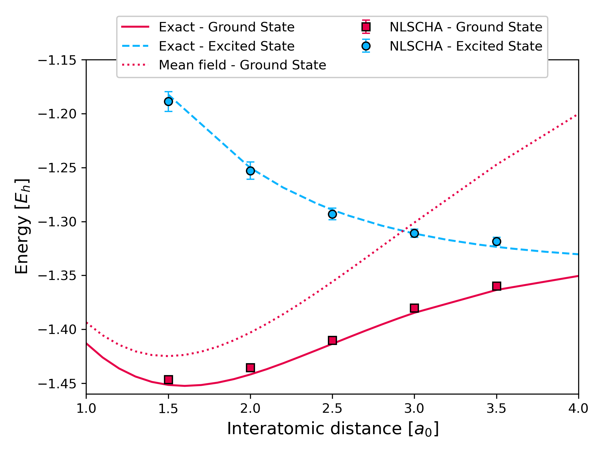
Fig. 6: Dissociation energies of H2. We compare the exact results obtained with numerical diagonalization of the Hamiltonian with the NLSCHA. The ground state is obtained in the singlet wave function, where both electrons have opposite spin in the ground state of the auxiliary harmonic oscillator. The excited state is the anti-bonding triplet solution, where one electron is in the ground state of the auxiliary harmonic Hamiltonian while the other is in the first excited state. The ground state’s mean-field energy (Hartree-Fock) is also reported as a reference.

The results are reported in Fig. 6, where we compare in red the NLSCHA with a six-layer transformation to the numerical exact diagonalization and the mean-field Hartree-Fock (HF) solution. As expected, HF reflects the problem of all mean-field approaches (as density functional theory) suffering from the static correlation error arising when the electrons localize on the atoms. The NLSCHA delivers an excellent agreement with the exact (numerical) result within the stochastic accuracy of the averages ($0.001\text{\,}\mathrm{\text{ $E_{\textup{ h }}$ }}$ in the ground state).

We benchmarked the antibonding excited state solution by promoting an electron to the first excited state of the auxiliary harmonic Hamiltonian in a triplet spin configuration. Notably, the H2 anti-bonding state is strongly affected by electron-hole interactions, as after the promotion of the electron in the excited state of the auxiliary Hamiltonian, the system significantly relaxes with dynamics similar to the one giving rise to excitonic states in condensed matter system. This state is challenging to capture even within GW: our method shows precision in the excitation gap within $0.2\text{\,}\mathrm{eV}$ across the whole dissociation curve, overcoming GW-BSE, which retains a similar accuracy only for $R<$2.3\text{\,}\mathrm{\text{ $a_{0}$ }}$$ Jing2021 . Therefore, the method displays promising potential for applications in materials with excitonic effects.

As the method is based on a first-principles quantization with a wavefunction approach, like VMC, we have an analytical expression for the resulting many-body wavefunction that we compare in Fig. 7 with the exact (full diagonalization) solution. The absence of spots in the principal diagonal of the colormaps (two electrons on the same atoms) indicates that the NLSCHA correctly accounts for correlation thanks to the off-diagonal elements in the $\bm{\Gamma}$ matrix of the Gaussian stretcher that couple the wavefunction of different electrons (Sec. VI), like a backflow transformation employed in Variational Monte Carlo (VMC).

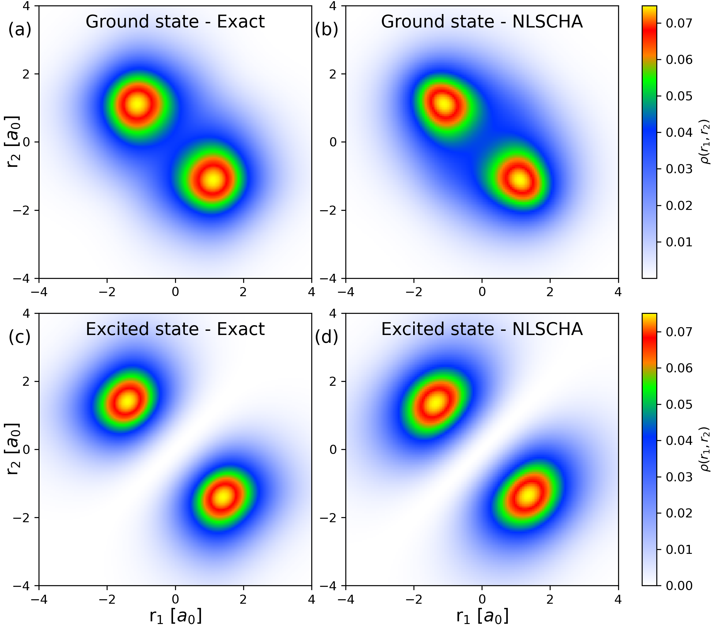
Fig. 7: 2-body electron density $\rho(r_{1},r_{2})$ for the H2 in dissociation ($d=$2.5\text{\,}\mathrm{\text{ $a_{0}$ }}$$) in the 1D soft-core Coulomb potential. (a) The ground state density evaluated with exact (numerical) diagonalization. (b) Ground state density evaluated within the NLSCHA, employing 6 layers in the nonlinear transformation from the Gaussian. (c) First excited state with exact (numerical) diagonalization. This is an anti-bonding state with the spins in the triplet configuration. (d) Excited state density computed with the NLSCHA, employing 2 layers in the nonlinear transformation from the Gaussian.

VIII Limits of the current implementation

In this section, we present the limits of the current implementation and discuss how they could be overcome.

As shown in Sec. VII.3, the method struggles to reproduce the electron-ion cusp, especially when large unscreened nuclear charges are in play (like for the case of core electrons), requiring a diverging number of hidden layers in the curved manifold. However, this is a common problem in electronic-structure simulations, e.g., in plane-wave basis sets, and has been solved a posteriori by employing pseudo potentials that smear out the electron-ion cusp near the nucleus. Also, the electron-electron cusp is likely to lead to numerical instabilities, and it is less clear how to fix it. However, due to its repulsive nature, the contribution of the exact wavefunction shape impacts the total energy much less as the many-body electron density goes to zero on the cusp.

The free energy minimization becomes more difficult as the number of layers in the neural network transformation increases. This is associated with the correlation between the parameters of the nested transformation performed by the multilayer Gaussian stretcher. A slight variation of parameters in some layers may cause a significative rearrangement of parameters in other layers, making it difficult to minimize the free energy efficiently. These limitations are in common with the standard Variational Monte Carlo (VMC) approaches, where they are overcome by preconditioning the algorithmSorella1998 . Preconditioning was also found to largely improve convergence in FermiNETPfau2020 , and it is currently employed in the stochastic implementation of the SCHA algorithmMonacelli2018 ; SSCHA , which is at the root of the recent success of the theory. Both VMC and SSCHA implementations also usually exploit a zero-variance principleAssaraf1999 for the free energy. In fact, already the use of a rescaled mass in the calculation of the kinetic energy improves the efficiency in the kinetic energy evaluation by order of magnitudes (see Appendix F). Exploring novel expressions for the kinetic and potential energy is expected to further improve the algorithm by strongly reducing the number of configurations required to converge. Last, different network architectures can be used to parameterize the curved manifold, like the Neural Ordinary Differential Equations (NODEs)NODEs and eventually stacked on top of the Gaussian stretchers.

IX Conclusions

The introduction of the SCHA in a curved manifold paved the way to systematically improve the variational solution of the SCHA while preserving the analytical solution of the auxiliary Harmonic system. In this work, we demonstrated how to build a curved manifold that can be iteratively improved by adding multiple hidden layers, like in a deep neural network. We also demonstrated how, thanks to this systematic improvement of the variational space, the SCHA can now tackle electrons in strongly correlated situations, like in the dissociation of H2. Even if the method shares a lot of similarities with other wavefunction approaches like the variational quantum Montecarlo, it remains a mean-field approach, as the interacting many-body Hamiltonian is mapped into a curved space where the wavefunction solves a noninteracting set of self-consistent harmonic oscillators. Since the standard SCHA can be derived in second quantizationALAMODE ; Tadano2022 ; Lihm2021 , and its self-energy is rigorously defined as an infinite resummation of Feynman diagramsMonacelli2021 ; SicilianoTSCHA2023 , the extension of this analysis to the SCHA within the curved manifold could pave the way for a systematic improvement of other mean-field approaches and the design of new exchange-correlation functional able to capture both the bounded and dissociated regimeGiesbertz2018 .

We not only introduced a new method to simulate both electrons and ions within the same theoretical framework, thus paving the way for fully nonadiabatic simulations, but we also unveiled its promising perspective in an only electron case. Indeed, we show how the Gaussian stretcher NLSCHA outperforms other mean-field approaches in describing strongly correlated systems, both in the ground and the excited state, thus providing a solid ground to investigate electron-phonon coupling beyond the Born-Oppenheimer approximation in correlated and magnetic materials.

Appendix A Kinetic energy

Here, we derive the kinetic energy:

$$K=-\sum_{i=1}^{N}\int\prod_{j}dR_{j}\psi^{\dagger}(\bm{R})\frac{\partial^{2}\psi}{\partial R_{i}^{2}}$$ (55)

Integrating by parts, we get

$$K=\sum_{i=1}^{N}\int\prod_{j}dR_{j}\frac{\partial\psi^{\dagger}}{\partial R_{i}}\frac{\partial\psi}{\partial R_{i}}$$ (56)

We can bring the density outside as

$$K=\sum_{i=1}^{N}\frac{1}{2m_{i}}\int\prod_{j}dR_{j}\rho(R)\frac{\partial\ln\psi^{\dagger}}{\partial R_{i}}\frac{\partial\ln\psi}{\partial R_{i}}$$ (57)

From which we have

$$\ln\psi=\ln\tilde{\psi}+\frac{1}{2}\ln\det\bm{J}$$ (58)

$$\frac{d\ln\psi}{dR_{a}} =\sum_{b}\frac{d\ln\tilde{\psi}}{dq_{b}}\frac{dq_{b}}{dR_{a}}+\frac{1}{2}\frac{d\ln\det\bm{J}}{dR_{a}}=$$

$$=\sum_{b}\frac{d\ln\tilde{\psi}}{dq_{b}}J_{ba}+\frac{1}{2}\sum_{cd}{\mathcal{J}}_{cd}J^{d}_{ca}$$ (59)

The overall kinetic energy is:

$$K=\sum_{i=1}^{N}\frac{1}{2m_{i}} \bigg{[}\sum_{bc}\left<J_{bi}J_{ci}\frac{d\ln{\tilde{\psi}}^{\dagger}}{dq_{b}}\frac{d\ln\tilde{\psi}}{dq_{c}}\right>$$

$$+\left<\left(\sum_{cd}{\mathcal{J}}_{cd}J^{d}_{ci}\right)\sum_{e}\frac{d\ln\tilde{\psi}}{dq_{e}}J_{ei}\right>$$

$$+\frac{1}{4}\left<\left(\sum_{cd}{\mathcal{J}}_{cd}J^{d}_{ci}\right)^{2}\right>\bigg{]},$$ (60)

from which we get the three observables:

$$\alpha_{i}(\bm{q})=\frac{1}{4}\left[\sum_{cd}{\mathcal{J}}_{cd}(\bm{q})J^{d}_{ci}(\bm{q})\right]^{2}$$ (61)

$$\beta_{i}^{e}(\bm{q})=J_{ei}(\bm{q})\left[\sum_{cd}{\mathcal{J}}_{cd}(\bm{q})J^{d}_{ci}(\bm{q})\right]$$ (62)

$$\gamma^{bc}_{i}(\bm{q})=J_{bi}(\bm{q})J_{ci}(\bm{q})$$ (63)

by exploiting the relation Eq. (86), we get:

$$\sum_{cd}{\mathcal{J}}_{cd}J^{d}_{ci}=-\sum_{ahk}J_{ha}J_{ki}{\mathcal{J}}^{a}_{kh}$$ (64)

This, indeed, works only for T = $0\text{\,}\mathrm{K}$; however, a similar approach can be derived also at finite temperature recognizing that:

$$K=-\sum_{i}\frac{1}{2m_{i}}\int\prod_{j}dR_{j}dR_{j}^{\prime}\delta(\bm{R}-\bm{R}^{\prime})\frac{\partial^{2}\rho(\bm{R},\bm{R}^{\prime})}{\partial{R^{\prime}}_{i}^{2}}$$ (65)

We can then exploit the integration by parts so that

$$K=\sum_{i}\frac{1}{2m_{i}}\int\prod_{j}dR_{j}dR_{j}^{\prime}\frac{\partial\delta(\bm{R}-\bm{R}^{\prime})}{\partial R^{\prime}_{i}}\frac{\partial\rho(\bm{R},\bm{R}^{\prime})}{\partial R^{\prime}_{i}}$$ (66)

Now we can exchange the derivative in the Dirac $\delta$ with $R$:

$$K=-\sum_{i}\frac{1}{2m_{i}}\int\prod_{j}dR_{j}dR_{j}^{\prime}\frac{\partial\delta(\bm{R}-\bm{R}^{\prime})}{\partial R_{i}}\frac{\partial\rho(\bm{R},\bm{R}^{\prime})}{\partial R^{\prime}_{i}}$$ (67)

And integrating back by parts

$$K=\sum_{i}\frac{1}{2m_{i}}\int\prod_{j}dR_{j}dR_{j}^{\prime}\delta(\bm{R}-\bm{R}^{\prime})\frac{\partial^{2}\rho(\bm{R},\bm{R}^{\prime})}{\partial R^{\prime}_{i}\partial R_{i}}.$$ (68)

This expression allows us to recover a symmetry and a single derivative on each variable that we can exploit:

$$\frac{\partial^{2}\rho(\bm{R},\bm{R}^{\prime})}{\partial R^{\prime}_{i}\partial R_{i}} =\sum_{h}\lambda_{h}\frac{\partial\psi_{h}}{\partial R_{i}}(\bm{R})\frac{\partial\psi_{h}^{\dagger}}{\partial R_{i}}(\bm{R}^{\prime})$$

$$=\sum_{h}\lambda_{h}\left|\psi_{h}\right|^{2}\frac{\partial\ln\psi_{h}}{\partial R_{i}}(\bm{R})\frac{\partial\ln\psi_{h}^{\dagger}}{\partial R_{i}}(\bm{R}^{\prime})$$ (69)

Now, the same procedure as in Eq. (59) can be exploited, where we end up with the same integrals as in Eq. (74), but where the averages are taken over each state in the mixture defined by the density matrix.

$$K=\sum_{i=1}^{N}\frac{1}{2m_{i}} \bigg{[}\sum_{bc}\int d\bm{q}J_{bi}J_{ci}\sum_{h}\lambda_{h}|\tilde{\psi}_{h}|^{2}\frac{d\ln{\tilde{\psi}_{h}}^{\dagger}}{dq_{b}}\frac{d\ln\tilde{\psi}_{h}}{dq_{c}}$$

$$+\int\left(\sum_{cd}{\mathcal{J}}_{cd}J^{d}_{ci}\right)\sum_{e}J_{ei}\sum_{h}\lambda_{h}|\tilde{\psi}_{h}|^{2}\frac{d\ln\tilde{\psi}_{h}}{dq_{e}}$$

$$+\frac{1}{4}\int\sum_{h}\lambda_{h}|\tilde{\psi}_{h}|^{2}\left(\sum_{cd}{\mathcal{J}}_{cd}J^{d}_{ci}\right)^{2}\bigg{]},$$ (70)

where

$$\sum_{h}\lambda_{h}|\tilde{\psi}_{h}|^{2}\frac{d\ln{\tilde{\psi}_{h}}^{\dagger}}{dq_{b}}\frac{d\ln\tilde{\psi}_{h}}{dq_{c}}=\int d\bm{q}^{\prime}\delta(\bm{q}-\bm{q}^{\prime})\frac{\partial^{2}\tilde{\rho}(\bm{q},\bm{q}^{\prime})}{\partial q_{b}\partial q_{c}^{\prime}}$$ (71)

$$\sum_{h}\lambda_{h}|\tilde{\psi}_{h}|^{2}\frac{d\ln\tilde{\psi}_{h}}{dq_{e}}=\int d\bm{q}^{\prime}\delta(\bm{q}-\bm{q}^{\prime})\frac{\partial\tilde{\rho}(\bm{q},\bm{q}^{\prime})}{\partial q_{e}^{\prime}}$$ (72)

$$\sum_{h}\lambda_{h}|\tilde{\psi}_{h}|^{2}=\tilde{\rho}(\bm{q})$$ (73)

$$K=\sum_{i=1}^{N}\frac{1}{2m_{i}} \bigg{[}\sum_{bc}\int d\bm{q}J_{bi}J_{ci}\int d\bm{q}^{\prime}\delta(\bm{q}-\bm{q}^{\prime})\frac{\partial^{2}\tilde{\rho}(\bm{q},\bm{q}^{\prime})}{\partial q_{b}\partial q_{c}^{\prime}}$$

$$+\int d\bm{q}\left(\sum_{cd}{\mathcal{J}}_{cd}J^{d}_{ci}\right)\sum_{e}J_{ei}\int d\bm{q}^{\prime}\delta(\bm{q}-\bm{q}^{\prime})\frac{\partial\tilde{\rho}(\bm{q},\bm{q}^{\prime})}{\partial q_{e}^{\prime}}$$

$$+\frac{1}{4}\left<\left(\sum_{cd}{\mathcal{J}}_{cd}J^{d}_{ci}\right)^{2}\right>\bigg{]},$$ (74)

Eq. (74) is the complete expression for the free energy, regardless of the auxiliary density matrix of choice $\tilde{\rho}(\bm{q},\bm{q}^{\prime})$. In the particular case of the Gaussian density matrix

$$\int d\bm{q}^{\prime}\delta(\bm{q}-\bm{q}^{\prime}) \frac{\partial^{2}\tilde{\rho}(\bm{q},\bm{q}^{\prime})}{\partial q_{a}\partial q_{b}}=\tilde{\rho}(\bm{q})\bigg{(}A_{ab}+$$

$$+\sum_{cd}\frac{\Upsilon_{ac}\Upsilon_{bd}}{4}(q_{c}-\mathcal{Q}_{c})(q_{d}-\mathcal{Q}_{d})\bigg{)},$$ (75)

$$\int d\bm{q}^{\prime}\delta(\bm{q}-\bm{q}^{\prime})\frac{\partial\tilde{\rho}(\bm{q},\bm{q}^{\prime})}{\partial q_{e}^{\prime}}=-\tilde{\rho}(\bm{q})\sum_{b}\frac{\Upsilon_{eb}}{2}(q_{b}-\mathcal{Q}_{b}),$$ (76)

that can be fit into the expression of Eq. (74) to evaluate numerically the kinetic energy.

Appendix B High-order jacobians of the single layer Gaussian Stretcher

To compute explicitly all the expression for the kinetic energy and the free energy gradients in the specific case of the Gaussian Stretcher transformation, we need to compute the Jacobian matrix up to the fourth order. We start with the single Gaussian stretcher

$${\mathcal{J}}_{ab}=\frac{dR_{a}}{dq_{b}}$$ (77)

$${\mathcal{J}}_{ab} =\delta_{ab}\left[1+(e^{\zeta}-1)e^{-\frac{1}{2}\tilde{\bm{q}}\bm{\Gamma}\tilde{\bm{q}}}\right]$$

$$-(e^{\zeta}-1)e^{-\frac{1}{2}\tilde{\bm{q}}\bm{\Gamma}\tilde{\bm{q}}}\sum_{c}\Gamma_{bc}(q_{c}-{\mathcal{Q}}_{c})(q_{a}-{\mathcal{Q}}_{a})$$ (78)

We can go on with further derivatives.

$${\mathcal{J}}^{a}_{bc}=\frac{dR_{a}}{dq_{b}dq_{c}}$$ (79)

$$\frac{{\mathcal{J}}^{a}_{bc}e^{\frac{1}{2}\tilde{\bm{q}}\bm{\Gamma}\tilde{\bm{q}}}}{(e^{\zeta}-1)} =-\delta_{ab}\sum_{h}\Gamma_{ch}(q_{h}-{\mathcal{Q}}_{h})-\delta_{ac}\sum_{h}\Gamma_{bh}(q_{h}-{\mathcal{Q}}_{h})$$

$$+\sum_{h}\Gamma_{bh}(q_{h}-{\mathcal{Q}}_{h})\sum_{k}\Gamma_{ck}(q_{k}-{\mathcal{Q}}_{k})(q_{a}-{\mathcal{Q}}_{a})$$

$$-\Gamma_{bc}(q_{a}-{\mathcal{Q}}_{a})$$ (80)

$$\frac{J^{a}_{bcd}e^{\frac{1}{2}\tilde{\bm{R}}\bm{\Gamma}\tilde{\bm{R}}}}{(e^{\zeta}-1)} =-\delta_{ab}\Gamma_{cd}-\delta_{ac}\Gamma_{bd}$$

$$-\delta_{ad}\Gamma_{bc}+\delta_{ad}(\bm{\Gamma}\tilde{\bm{q}})_{b}(\bm{\Gamma}\tilde{\bm{q}})_{c}$$

$$+\tilde{q}_{a}\Gamma_{bd}(\bm{\Gamma}\tilde{\bm{q}})_{c}+\tilde{q}_{a}\Gamma_{cd}(\bm{\Gamma}\tilde{\bm{q}})_{b}$$

$$+\delta_{ab}(\bm{\Gamma}\tilde{\bm{q}})_{d}(\bm{\Gamma}\tilde{\bm{q}})_{c}+\delta_{ac}(\bm{\Gamma}\tilde{\bm{q}})_{b}(\bm{\Gamma}\tilde{\bm{q}})_{d}$$

$$+\tilde{q}_{a}\Gamma_{bc}(\bm{\Gamma}\tilde{\bm{q}})_{d}-\tilde{q}_{a}(\bm{\Gamma}\tilde{\bm{q}})_{b}(\bm{\Gamma}\tilde{\bm{q}})_{c}(\bm{\Gamma}\tilde{\bm{q}})_{d}$$ (81)

Appendix C high-order jacobians of the multilayer Gaussian stretcher

As suggested in the main text, nonlinear transformations can be concatenated to form more complex transformations. We can derive the jacobian by using the composite transformation:

$$\frac{d}{dq_{j}}q^{(m)}_{i}(q_{1}^{(m-1)},\cdots,q_{n}^{(m-1)})=\sum_{a=1}^{n}\frac{dq^{(m)}_{i}}{dq_{a}^{(m-1)}}\frac{dq_{a}^{(m-1)}}{dq_{j}}$$ (82)

From which we get a recursive equation

$${\mathcal{J}}_{ij}^{(m)}=\sum_{a}{\mathcal{J}}_{ia}(\bm{q}^{(m-1)}){\mathcal{J}}_{aj}^{(m-1)}(\bm{q}^{(1)})$$ (83)

Which means that the jacobian is the matrix product of the jacobians after each iteration. The second order jacobian becomes

$$({\mathcal{J}}^{(m)})^{i}_{jk}= \sum_{ab}{\mathcal{J}}^{i}_{ab}(\bm{q}^{(m-1)}){\mathcal{J}}^{(m-1)}_{aj}{\mathcal{J}}^{(m-1)}_{bk}+$$

$$\sum_{a}{\mathcal{J}}_{ia}(\bm{q}^{(m-1)})({\mathcal{J}}^{(m-1)})^{a}_{jk}$$ (84)

And the higher-order derivative becomes

$$({\mathcal{J}}^{(m)})^{i}_{jkh}= \sum_{abc}{\mathcal{J}}^{i}_{abc}(\bm{q}^{(m-1)}){\mathcal{J}}^{(m-1)}_{aj}{\mathcal{J}}^{(m-1)}_{bk}{\mathcal{J}}^{(m-1)}_{ch}+$$

$$\sum_{ab}{\mathcal{J}}^{i}_{ab}(\bm{q}^{(m-1)})\left({\mathcal{J}}^{(m-1)}\right)^{a}_{jh}{\mathcal{J}}^{(m-1)}_{bk}+$$

$$\sum_{ab}{\mathcal{J}}^{i}_{ab}(\bm{q}^{(m-1)}){\mathcal{J}}^{(m-1)}_{aj}\left({\mathcal{J}}^{(m-1)}\right)^{b}_{kh}+$$

$$\sum_{ab}{\mathcal{J}}^{i}_{ab}(\bm{q}^{(m-1)}){\mathcal{J}}^{(m-1)}_{bh}({\mathcal{J}}^{(m-1)})^{a}_{jk}+$$

$$\sum_{a}{\mathcal{J}}_{ia}(\bm{q}^{(m-1)})\left({\mathcal{J}}^{(m-1)}\right)^{a}_{jkh}$$ (85)

This chain rule allows the computation of all the jacobians as a forward propagation algorithm. This scheme can be seen as a neural network with a gaussian activation function.

Appendix D Some useful relations

We simplify some explicit multiplication between Jacobians that often appear in the derivations. For example, in the expression for $\beta^{i}_{a}(\bm{q})$ we find the multiplication:

$$\sum_{cd}{\mathcal{J}}_{cd}J^{d}_{ca}=-\sum_{hkl}J_{kh}J_{la}{\mathcal{J}}^{h}_{kl}$$ (86)

In the same way, for $\alpha$ is important the following multiplication

$$\sum_{bc}{\mathcal{J}}_{bc}J^{c}_{baa}=-\sum_{hkl} \bigg{[}J_{kh}J_{la}\sum_{m}{\mathcal{J}}^{h}_{lkm}J_{ma}+$$

$$+2J^{k}_{ha}J_{la}{\mathcal{J}}^{h}_{lk}+J_{kh}J^{l}_{aa}{\mathcal{J}}^{h}_{lk}\bigg{]}$$ (87)

Appendix E Harmonic oscillator of Fermions

Here, we report the solution of the harmonic Hamiltonian for fermions. The system is composed of $N$ fermions interacting within a harmonic potential. For simplicity, we consider a one-dimensional space. Due to the exchange symmetry, in 1D there are only 2 degrees of freedom: the self-interaction $a$ and electronic repulsion $b$

$$V(q_{1},\cdots,q_{N})=\frac{1}{2}a\sum_{i=1}^{N}q_{i}^{2}-\frac{1}{2}b\sum_{ij}(q_{i}-q_{j})^{2}.$$ (88)

Reorganizing the terms of the equation, we get

$$V(q_{1},\cdots,q_{N})=\frac{1}{2}\left(a-b\right)\sum_{i=1}^{N}q_{i}^{2}-b\sum_{i\neq j}q_{i}q_{j},$$ (89)

$$V(\bm{q})=\frac{1}{2}\begin{pmatrix}q_{1}&\cdots&q_{N}\end{pmatrix}\begin{pmatrix}(a-b)&-b&\cdots&-b\\ -b&(a-b)&\cdots&-b\\ \vdots&\vdots&\ddots&\vdots\\ -b&\cdots&-b&(a-b)\end{pmatrix}\begin{pmatrix}q_{1}\\ \vdots\\ q_{N}\end{pmatrix}$$ (90)

This is an interacting problem that can be trivially solved by diagonalizing the matrix. The solution have 2 eigenvalues

$$\lambda_{1}=a-Nb\qquad\bm{e_{1}}=\begin{pmatrix}1\\ \vdots\\ 1\end{pmatrix},$$ (91)

$$\lambda_{2},\cdots,\lambda_{n}=a\qquad\bm{e_{2}}=\begin{pmatrix}1\\ -1\\ 0\\ \vdots\\ 0\end{pmatrix},\cdots,\bm{e_{N}}=\begin{pmatrix}1\\ 0\\ \vdots\\ 0\\ -1\end{pmatrix}.$$ (92)

The eigenvector $\bm{e_{1}}$ is already symmetric under the exchange of any couple of particles, each $\bm{e_{i}}$ with $i\geq 2$ is antisymmetric for exchanging two specific particles and symmetric for exchanging any other 2. Unfortunately, for more than 2 particles, it is impossible to build a basis from $\bm{e_{2}},\cdots,\bm{e_{n}}$ that commutes with all the exchange operators $\bm{S_{ij}}$. While we know the spectrum of the problem, this makes it very difficult to find exact selection rules to populate states in the case of fermions and bosons for more than 2 particles, in particular, if we also account for the spin degrees of freedom. Another problem arises in the thermodynamic limit $N\rightarrow\infty$. In this case, the spectrum, and in particular $\lambda_{1}$ (Eq. 91), becomes not positive definite for any small positive value of $b$. Thus, even if the Harmonic Hamiltonian may describe the correlation of molecules or systems with a finite number of electrons, $b\rightarrow 0$ in the thermodynamic limit, we recover a noninteracting Hamiltonian. For this reason, in the main text, we restrict to the noninteracting case where $b=0$.

Appendix F Position dependent effective mass tensor

As in classical Lagrange equations, the constrained motion on a curved manifold affects the effective masses of the systems. In classical mechanics, the kinetic energy after the change of variable is obtained as:

$$K_{\text{cl}}=\sum_{i}\frac{1}{2m_{i}}\left<J_{ai}J_{bi}p_{a}p_{b}\right>$$ (93)

where $p_{a}$ is the $a$-th component of the moment of the auxiliary variable $q_{a}$. The transformation of the variable thus can be seen as a mass that depends on the metric tensor:

$$M^{-1}_{ab}=\sum_{i}\frac{J_{ai}J_{bi}}{m_{i}}$$ (94)

$$K_{\text{cl}}=\frac{1}{2}\sum_{ab}\left<p_{a}M^{-1}_{ab}p_{b}\right>.$$ (95)

Unfortunately, in quantum mechanics, it is not possible to quantize directly the auxiliary variables and thus express everything as a simple change of masses. However, we can always write the kinetic energy as

$$K=K_{\text{cl}}+K_{\text{cor}}$$ (96)

where $K_{\text{cor}}$ is the quantum correction to the kinetic energy. In particular, from Eq. (31), the term that contains Eq. (95) is the one that multiplies the $\bm{\gamma}$ tensor.

$$K_{\text{cor}}=-\sum_{a=1}^{3N} \frac{\hbar^{2}}{2m_{a}}\left<\alpha^{a}(\bm{q})+\sum_{i}\beta^{a}_{i}(\bm{q})\hat{P}_{i}\right>$$ (97)

Since in practice, the classical kinetic energy is both the biggest part of the kinetic energy and the one with the highest noise, it is convenient to rewrite it as the masses are constant (linear transformation) and average only the curvature:

$$\bar{M}^{-1}_{ab}=\left<M^{-1}_{ab}(\bm{q})\right>\qquad\Delta M^{-1}_{ab}(\bm{q})=M^{-1}_{ab}(\bm{q})-\bar{M}^{-1}_{ab}$$ (98)

$$K_{\text{cl}}=\frac{1}{2}\sum_{ab}\bar{M}^{-1}_{ab}\left<p_{a}p_{b}\right>+\frac{1}{2}\sum_{ab}\left<p_{a}\Delta M^{-1}_{ab}(\bm{q})p_{b}\right>.$$ (99)

where the first term is analytical when for Gaussian wavefunctions in the auxiliary system. The evaluation of the classical kinetic energy through Eq. (99) strongly suppresses the stochastic noise compared with Eq. (93), but it has the same expected value.

Appendix G Fermionic and bosonic wavefunction

Up to two electrons, the wave function remains symmetric as it can be described by a singlet state, where the antisymmetric part of the wave function is trivially encoded by their opposed spin. However, the factorization of space and spin for the exchange symmetry is only possible for two electrons. Therefore, to solve a realistic system beyond the Helium atom or the H2 molecule it is necessary to devise a new strategy to encode the antisymmetry of the wavefunction.

In the opening of Sec. VI, we derived the constraint on the nonlinear transformation to keep the exchange symmetry of the wavefunction in the auxiliary variables throughout the nonlinear transformation operated by the neural network. Here, we devise a way to account for a fermionic (or bosonic) wavefunction directly in the auxiliary space.

The only requirements is to be able to:

• Extract random configurations according to the correct statistics.

• Evaluate the modified kinetic energy average in the auxiliary space (Eq. 97 and 95)

To extract random configurations distributed according to the Fermi-Dirac, we employ a standard quantum Monte Carlo algorithm sampling the wavefunction $\Psi(q)$ as the Slater determinant of the harmonic eigenfunctions.

Storing for each configuration in $q$ space the gradient of the wavefunction, we can easily compute the averages of kinetic operators that depends on both $P$ and $q$:

$$i\hbar\left<\beta_{a}(\bm{q})P_{a}\right>=-\hbar^{2}\left<\beta_{a}(\bm{q})\frac{\partial\ln\Psi}{\partial q_{a}}\right>$$ (100)

$$\left<P_{a}\gamma_{ab}(q)P_{b}\right>=\hbar^{2}\left<\gamma_{ab}(\bm{q})\frac{\partial\ln\Psi^{*}}{\partial q_{a}}\frac{\partial\ln\Psi}{\partial q_{b}}\right>$$ (101)

Which is equivalent to substituting the ${\bm{\Upsilon}}\bm{q}$ with $\nabla_{\bm{q}}\ln\Psi$ from the equations of the standard SSCHA. Interestingly, the derivative of the logarithm of the wavefunction is independent on its global phase, thus, Eq. (100) satisfies the Gauge invariance. Indeed, if the global phase depends on the position, care must be taken as Eq. (100) could be related to topological phenomena. Therefore, we must store, for each point in the auxiliary ensemble, the value of the gradient of the logarithm of the slater determinant, which can be evaluated efficiently using algorithmic differentiation. The analytical value of the kinetic energy in a pure state can be evaluated as

$$\braket{P_{a}P_{b}}=\frac{1}{N_{e}}\delta_{ab}\frac{\hbar}{2}\sum_{\mu=0}^{\infty}\left[2n_{\mu}+1\right]f_{\mu}$$ (102)

where $f_{\mu}$ now indicate the number of electrons occupying the $n_{\mu}$ state of the auxiliary harmonic Hamiltonian along the $a$ or $b$ direction.

References

- (1) N. Marzari, A. Ferretti, and C. Wolverton, “Electronic-structure methods for materials design,” vol. 20, no. 6, pp. 736–749. Publisher: Nature Publishing Group.
- (2) P. Hohenberg and W. Kohn, “Inhomogeneous electron gas,” vol. 136, no. 3, pp. B864–B871. Publisher: American Physical Society.
- (3) K. Burke and L. O. Wagner, “DFT in a nutshell,” vol. 113, no. 2, pp. 96–101.
- (4) A. Georges, G. Kotliar, W. Krauth, and M. J. Rozenberg, “Dynamical mean-field theory of strongly correlated fermion systems and the limit of infinite dimensions,” Rev. Mod. Phys., vol. 68, pp. 13–125, Jan 1996.
- (5) L. Monacelli, I. Errea, M. Calandra, and F. Mauri, “Black metal hydrogen above 360 GPa driven by proton quantum fluctuations,” Nat. Phys., vol. 17, pp. 63–67, sep 2020.
- (6) L. Monacelli, M. Casula, K. Nakano, S. Sorella, and F. Mauri, “Quantum phase diagram of high-pressure hydrogen,” Nature Physics, vol. 19, p. 845–850, Mar. 2023.
- (7) I. Errea, M. Calandra, C. J. Pickard, J. R. Nelson, R. J. Needs, Y. Li, H. Liu, Y. Zhang, Y. Ma, and F. Mauri, “Quantum hydrogen-bond symmetrization in the superconducting hydrogen sulfide system,” Nature, vol. 532, pp. 81–84, mar 2016.
- (8) I. Errea, F. Belli, L. Monacelli, A. Sanna, T. Koretsune, T. Tadano, R. Bianco, M. Calandra, R. Arita, F. Mauri, and J. A. Flores-Livas, “Quantum crystal structure in the 250-kelvin superconducting lanthanum hydride,” Nature, vol. 578, pp. 66–69, feb 2020.
- (9) J. A. Morrone and R. Car, “Nuclear quantum effects in water,” Phys. Rev. Lett., vol. 101, p. 017801, Jul 2008.
- (10) M. Cherubini, L. Monacelli, and F. Mauri, “The microscopic origin of the anomalous isotopic properties of ice relies on the strong quantum anharmonic regime of atomic vibration,” J. Chem. Phys., vol. 155, p. 184502, nov 2021.
- (11) U. Ranieri, S. Di Cataldo, M. Rescigno, L. Monacelli, R. Gaal, M. Santoro, L. Andriambariarijaona, P. Parisiades, C. De Michele, and L. E. Bove, “Observation of the most h 2 -dense filled ice under high pressure,” Proceedings of the National Academy of Sciences, vol. 120, Dec. 2023.
- (12) M. Cherubini, L. Monacelli, B. Yang, R. Car, M. Casula, and F. Mauri, “Quantum effects in the h-bond symmetrization and in the thermodynamic properties of high pressure ice,” arXiv preprint arXiv:2403.09238, 2024.
- (13) L. Binci, P. Barone, and F. Mauri, “First-principles theory of infrared vibrational spectroscopy of metals and semimetals: Application to graphite,” Phys. Rev. B, vol. 103, p. 134304, Apr 2021.
- (14) G. Marchese, F. Macheda, L. Binci, M. Calandra, P. Barone, and F. Mauri, “Born effective charges and vibrational spectra in superconducting and bad conducting metals,” Nature Physics, vol. 20, p. 88–94, Oct. 2023.
- (15) N. Girotto and D. Novko, “Dynamical renormalization of electron-phonon coupling in conventional superconductors,” Phys. Rev. B, vol. 107, p. 064310, Feb 2023.
- (16) C.-J. Tong, X. Cai, A.-Y. Zhu, L.-M. Liu, and O. V. Prezhdo, “How hole injection accelerates both ion migration and nonradiative recombination in metal halide perovskites,” Journal of the American Chemical Society, vol. 144, p. 6604–6612, Apr. 2022.
- (17) Y. J. Uemura, G. M. Luke, B. J. Sternlieb, J. H. Brewer, J. F. Carolan, W. N. Hardy, R. Kadono, J. R. Kempton, R. F. Kiefl, S. R. Kreitzman, P. Mulhern, T. M. Riseman, D. L. Williams, B. X. Yang, S. Uchida, H. Takagi, J. Gopalakrishnan, A. W. Sleight, M. A. Subramanian, C. L. Chien, M. Z. Cieplak, G. Xiao, V. Y. Lee, B. W. Statt, C. E. Stronach, W. J. Kossler, and X. H. Yu, “Universal correlations between and (carrier density over effective mass) in high- cuprate superconductors,” Phys. Rev. Lett., vol. 62, pp. 2317–2320, May 1989.
- (18) J. C. Tully, “Molecular dynamics with electronic transitions,” The Journal of Chemical Physics, vol. 93, p. 1061–1071, July 1990.
- (19) P. Nijjar, J. Jankowska, and O. V. Prezhdo, “Ehrenfest and classical path dynamics with decoherence and detailed balance,” The Journal of Chemical Physics, vol. 150, May 2019.
- (20) C. F. Craig, W. R. Duncan, and O. V. Prezhdo, “Trajectory surface hopping in the time-dependent kohn-sham approach for electron-nuclear dynamics,” Phys. Rev. Lett., vol. 95, p. 163001, Oct 2005.
- (21) L. Wang, A. Akimov, and O. V. Prezhdo, “Recent progress in surface hopping: 2011–2015,” The Journal of Physical Chemistry Letters, vol. 7, p. 2100–2112, May 2016.
- (22) P. Shushkov, R. Li, and J. C. Tully, “Ring polymer molecular dynamics with surface hopping,” The Journal of Chemical Physics, vol. 137, Nov. 2012.
- (23) D. M. Ceperley, “Path integrals in the theory of condensed helium,” Reviews of Modern Physics, vol. 67, no. 2, pp. 279–355, 1995.
- (24) K. P. Driver and B. Militzer, “All-electron path integral monte carlo simulations of warm dense matter: Application to water and carbon plasmas,” Phys. Rev. Lett., vol. 108, p. 115502, Mar 2012.
- (25) I. Errea, M. Calandra, and F. Mauri, “Anharmonic free energies and phonon dispersions from the stochastic self-consistent harmonic approximation: Application to platinum and palladium hydrides,” Physical Review B, vol. 89, p. 064302, Feb. 2014.
- (26) L. Monacelli and F. Mauri, “Time-dependent self-consistent harmonic approximation: Anharmonic nuclear quantum dynamics and time correlation functions,” Physical Review B, vol. 103, p. 104305, Mar. 2021.
- (27) M. Miotto and L. Monacelli, “Fast prediction of anharmonic vibrational spectra for complex organic molecules,” vol. 10, no. 1, pp. 1–9. Publisher: Nature Publishing Group.
- (28) M. Borinaga, P. Riego, A. Leonardo, M. Calandra, F. Mauri, A. Bergara, and I. Errea, “Anharmonic enhancement of superconductivity in metallic molecular cmca4 hydrogen at high pressure: a first-principles study,” Journal of Physics: Condensed Matter, vol. 28, p. 494001, Oct. 2016.
- (29) M. Borinaga, I. Errea, M. Calandra, F. Mauri, and A. Bergara, “Anharmonic effects in atomic hydrogen: Superconductivity and lattice dynamical stability,” Phys. Rev. B, vol. 93, p. 174308, May 2016.
- (30) L. Monacelli and N. Marzari, “First-principles thermodynamics of cssni3,” Chemistry of Materials, vol. 35, p. 1702–1709, Feb. 2023.
- (31) J. S. Zhou, R. Bianco, L. Monacelli, I. Errea, F. Mauri, and M. Calandra, “Theory of the thickness dependence of the charge density wave transition in 1 t-TiTe2,” 2D Mater., vol. 7, p. 045032, sep 2020.
- (32) R. Bianco, I. Errea, L. Monacelli, M. Calandra, and F. Mauri, “Quantum enhancement of charge density wave in NbS2 in the two-dimensional limit,” Nano Lett., vol. 19, pp. 3098–3103, apr 2019.
- (33) R. Bianco, L. Monacelli, M. Calandra, F. Mauri, and I. Errea, “Weak dimensionality dependence and dominant role of ionic fluctuations in the charge-density-wave transition of ,” Phys. Rev. Lett., vol. 125, p. 106101, Sep 2020.
- (34) J. Diego, A. H. Said, S. K. Mahatha, R. Bianco, L. Monacelli, M. Calandra, F. Mauri, K. Rossnagel, I. Errea, and S. Blanco-Canosa, “van der waals driven anharmonic melting of the 3d charge density wave in VSe2,” Nature Communications, vol. 12, p. 598, jan 2021.
- (35) A. Siciliano, L. Monacelli, and F. Mauri, “Beyond gaussian fluctuations of quantum anharmonic nuclei.”
- (36) A. Siciliano, L. Monacelli, and F. Mauri, “Beyond gaussian fluctuations of quantum anharmonic nuclei: The case of rotational degrees of freedom,” vol. 110, no. 14, p. 144101.
- (37) L. Monacelli, R. Bianco, M. Cherubini, M. Calandra, I. Errea, and F. Mauri, “The stochastic self-consistent harmonic approximation: calculating vibrational properties of materials with full quantum and anharmonic effects,” Journal of Physics: Condensed Matter, vol. 33, p. 363001, July 2021.
- (38) W. M. C. Foulkes, L. Mitas, R. J. Needs, and G. Rajagopal, “Quantum monte carlo simulations of solids,” vol. 73, no. 1, pp. 33–83.
- (39) U. Aseginolaza, R. Bianco, L. Monacelli, L. Paulatto, M. Calandra, F. Mauri, A. Bergara, and I. Errea, “Phonon collapse and second-order phase transition in thermoelectric SnSe,” Physical Review Letters, vol. 122, p. 075901, Feb. 2019.
- (40) C. Verdi, L. Ranalli, C. Franchini, and G. Kresse, “Quantum paraelectricity and structural phase transitions in strontium titanate beyond density functional theory,” vol. 7, no. 3, p. L030801.
- (41) D. Romanin, L. Monacelli, R. Bianco, I. Errea, F. Mauri, and M. Calandra, “Dominant role of quantum anharmonicity in the stability and optical properties of infinite linear acetylenic carbon chains,” J. Phys. Chem. Lett., vol. 12, pp. 10339–10345, oct 2021.
- (42) L. Ranalli, C. Verdi, L. Monacelli, G. Kresse, M. Calandra, and C. Franchini, “Temperature-dependent anharmonic phonons in quantum paraelectric KTaO3 by first principles and machine-learned force fields,” vol. 6, no. 4, p. 2200131. _eprint: https://onlinelibrary.wiley.com/doi/pdf/10.1002/qute.202200131.
- (43) A. Pedrielli, P. E. Trevisanutto, L. Monacelli, G. Garberoglio, N. M. Pugno, and S. Taioli, “Understanding anharmonic effects on hydrogen desorption characteristics of mgnh2 nanoclusters by ab initio trained deep neural network,” Nanoscale, vol. 14, no. 14, pp. 5589–5599, 2022.
- (44) D. P. Kingma and J. Ba, “Adam: A method for stochastic optimization,” CoRR, vol. abs/1412.6980, 2014.
- (45) D. C. S. R. B. Lehoucq and C. Yang, ARPACK USERS GUIDE: Solution of Large Scale Eigenvalue Problems by Implicitly Restarted Arnoldi Methods. SIAM, Philadelphia, PA, 1998.
- (46) P. Virtanen, R. Gommers, T. E. Oliphant, M. Haberland, T. Reddy, D. Cournapeau, E. Burovski, P. Peterson, W. Weckesser, J. Bright, S. J. van der Walt, M. Brett, J. Wilson, K. J. Millman, N. Mayorov, A. R. J. Nelson, E. Jones, R. Kern, E. Larson, C. J. Carey, İ. Polat, Y. Feng, E. W. Moore, J. VanderPlas, D. Laxalde, J. Perktold, R. Cimrman, I. Henriksen, E. A. Quintero, C. R. Harris, A. M. Archibald, A. H. Ribeiro, F. Pedregosa, P. van Mulbregt, and SciPy 1.0 Contributors, “SciPy 1.0: Fundamental Algorithms for Scientific Computing in Python,” Nature Methods, vol. 17, pp. 261–272, 2020.
- (47) A. Cuzzocrea, A. Scemama, W. J. Briels, S. Moroni, and C. Filippi, “Variational principles in quantum monte carlo: The troubled story of variance minimization,” Journal of Chemical Theory and Computation, vol. 16, pp. 4203–4212, May 2020.
- (48) M. Dash, J. Feldt, S. Moroni, A. Scemama, and C. Filippi, “Excited states with selected configuration interaction-quantum monte carlo: Chemically accurate excitation energies and geometries,” Journal of Chemical Theory and Computation, vol. 15, pp. 4896–4906, July 2019.
- (49) T. Kato, “On the eigenfunctions of many-particle systems in quantum mechanics,” Communications on Pure and Applied Mathematics, vol. 10, no. 2, pp. 151–177, 1957.
- (50) T. Olsen and K. S. Thygesen, “Static correlation beyond the random phase approximation: Dissociating h2 with the bethe-salpeter equation and time-dependent gw,” The Journal of Chemical Physics, vol. 140, Apr. 2014.
- (51) K. J. H. Giesbertz, A.-M. Uimonen, and R. van Leeuwen, “Approximate energy functionals for one-body reduced density matrix functional theory from many-body perturbation theory,” The European Physical Journal B, vol. 91, Nov. 2018.
- (52) R. L. Hall, N. Saad, K. D. Sen, and H. Ciftci, “Energies and wave functions for a soft-core coulomb potential,” Phys. Rev. A, vol. 80, p. 032507, Sep 2009.
- (53) M. Iñarrea, V. Lanchares, J. F. Palacián, A. I. Pascual, J. P. Salas, and P. Yanguas, “Effects of a soft-core coulomb potential on the dynamics of a hydrogen atom near a metal surface,” Communications in Nonlinear Science and Numerical Simulation, vol. 68, pp. 94–105, Mar. 2019.
- (54) J. Li and V. Olevano, “Hydrogen-molecule spectrum by the many-body approximation and the bethe-salpeter equation,” Phys. Rev. A, vol. 103, p. 012809, Jan 2021.
- (55) S. Sorella, “Green function monte carlo with stochastic reconfiguration,” Phys. Rev. Lett., vol. 80, pp. 4558–4561, May 1998.
- (56) D. Pfau, J. S. Spencer, A. G. D. G. Matthews, and W. M. C. Foulkes, “Ab initio solution of the many-electron schrödinger equation with deep neural networks,” Phys. Rev. Res., vol. 2, p. 033429, Sep 2020.
- (57) L. Monacelli, I. Errea, M. Calandra, and F. Mauri, “Pressure and stress tensor of complex anharmonic crystals within the stochastic self-consistent harmonic approximation,” Physical Review B, vol. 98, p. 024106, July 2018.
- (58) R. Assaraf and M. Caffarel, “Zero-variance principle for monte carlo algorithms,” Physical Review Letters, vol. 83, p. 4682–4685, Dec. 1999.
- (59) R. T. Q. Chen, Y. Rubanova, J. Bettencourt, and D. K. Duvenaud, “Neural ordinary differential equations,” Advances in Neural Information Processing Systems, vol. 31, pp. 6571–6583, 2018.
- (60) T. Tadano, Y. Gohda, and S. Tsuneyuki, “Anharmonic force constants extracted from first-principles molecular dynamics: applications to heat transfer simulations,” J. Phys.: Condens. Matter, vol. 26, p. 225402, may 2014.
- (61) T. Tadano and W. A. Saidi, “First-principles phonon quasiparticle theory applied to a strongly anharmonic halide perovskite,” Physical Review Letters, vol. 129, p. 185901, Oct. 2022.
- (62) J.-M. Lihm and C.-H. Park, “Gaussian time-dependent variational principle for the finite-temperature anharmonic lattice dynamics,” Phys. Rev. Res., vol. 3, p. L032017, Jul 2021.
- (63) A. Siciliano, L. Monacelli, G. Caldarelli, and F. Mauri, “Wigner gaussian dynamics: Simulating the anharmonic and quantum ionic motion,” Phys. Rev. B, vol. 107, p. 174307, May 2023.