Online design of dynamic networks

Abstract

Designing a network (e.g., a telecommunication or transport network) is mainly done offline, in a planning phase, prior to the operation of the network. On the other hand, a massive effort has been devoted to characterizing dynamic networks, i.e., those that evolve over time. The novelty of this paper is that we introduce a method for the online design of dynamic networks. The need to do so emerges when a network needs to operate in a dynamic and stochastic environment. In this case, one may wish to build a network over time, on the fly, in order to react to the changes of the environment and to keep certain performance targets. We tackle this online design problem with a rolling horizon optimization based on Monte Carlo Tree Search. The potential of online network design is showcased for the design of a futuristic dynamic public transport network, where bus lines are constructed on the fly to better adapt to a stochastic user demand. In such a scenario, we compare our results with state-of-the-art dynamic vehicle routing problem (VRP) resolution methods, simulating requests from a New York City taxi dataset. Differently from classic VRP methods, that extend vehicle trajectories in isolation, our method enables us to build a structured network of line buses, where complex user journeys are possible, thus increasing system performance.

Keywords Dynamic Network  $\cdot$ Design  $\cdot$ Online Design Problem  $\cdot$ Monte Carlo Tree Search  $\cdot$ Public Transport Network

1 Introduction

Methods for network designs are generally only aimed at static networks [1, 2]. They usually assume a fixed structure of graphs. However, these graphs are far from the real world. However, real-world networks are dynamic. For example, friend relationships in social networks are added or deleted over time, and transport systems often change over time. These dynamics can be captured by Temporal Graphs (TGs), which can change over time. TGs have been adopted to model transport systems [3, 4], social networks [5], recommendation systems [6] and many others [7, 8, 9].

Previous works focus on analyzing TGs, or on solving problems on top of a TG with exogenous time-evolution. To the best of our knowledge, this paper is the first to tackle the design of TGs. Differently from previous work, where dynamics are exogenous, we wish instead to determine such dynamics to optimize some objective function, faced with some random and time-varying environment. We focus in particular on a particular class of TGs, namely Time-Expanded Graphs.

Our main contributions are the following:

• We introduce the problem of designing dynamic graphs, while previous work has focused only on their analysis.

• We propose an online decision process to perform such a design task, based on a rolling horizon approach.

• We adapt Monte Carlo Tree Search (MCTS) to the case of building Time-Expanded Graphs (TEGs) to maximize reward in a stochastic environment. Our method relies on a model of the environment, which predicts, online, the impact of certain design actions. This allows to build a TEG, online, that adapts to the environment.

• We apply our approach to the transport domain, where a stochastic sequence of trip requests need to be served by a fleet of buses and we show we outperform the state of the art (SOTA).

As for the transport application, the SOTA relies in Vehicle Routing Problem (VRP) methods, which route vehicles one by one. Resulting vehicle trajectories thus lack structure. On the contrary, our method enables us to build a network of bus lines, which features a structure. Therefore, users can navigate such a network and make transfers from a line to another. Thanks to structure, our system is able to serve more requests with a smaller fleet. Results are obtained on a dataset of trip requests in New York.

We believe that our approach provides inspiration for designing dynamic networks performing in a stochastic environment without a-priori knowledge. Our code is available as open source [10].

2 Related Work

We first frame our approach in the context of the research work on Temporal Graphs. Since we also apply our method to a transport case, we also briefly review the related literature.

2.1 Dynamic graphs

Temporal Graphs (TGs) are graphs that evolve over time. Several types of temporal graphs exist. Two main types of evolution have been mainly considered. (1) Label evolution refers to changes of attributes associated to edges and/or vertices. (2) Topological evolution refers to changes in a graph topology (for instance, nodes and edges appear or disappear over time). We focus on the latter category in this paper and whenever we write Temporal Graph (TG), we refer just to this latter category.

A review of the literature on TGs is provided in [11]. Currently, the main research tasks considered for TGs are mining frequent subgraphs [12, 13], mining periodic patterns [14], finding association rules [15], mining motifs [16] and temporal link prediction [17]. Temporal Graph Neural Networks (TGNNs) have achieved state-of-the-art results in the above problems [17]. The main purpose of the above studies is “observation”, i.e., to learn some common patterns, for example common frequent subgraphs, in TGs or analyze some statistical properties. More precisely, given a TG $\pazocal G=\{\pazocal G_{t-N},\pazocal G_{t-N+1},\dots,\pazocal G_{t}\}$, they try to find some common patterns in the current state and then verify these patterns in the next state $\pazocal G=\{\pazocal G_{t-N},\pazocal G_{t-N+1},\dots,\pazocal G_{t+1}\}$. These studies attempt to observe some common characteristics in the evolution of TGs without such an evolution.

In other work, on top of an evolving network modeled via TG, a certain optimization problem is solved [18, 19]. In this case, the decision variables of such problems do not impact network evolution, rather they have to “cope with” network evolution. In other words, in such work, network evolution is exogenous. In this paper, we are interested instead in designing network evolution ourselves. In other words, we do not perform some tasks on a network that is evolving out of our control, but we instead construct a temporal network. To emphasize the idea of construction over time, we will say that we grow a TG. This case is particularly important when dealing with dynamic networks such as communication or transport networks. In such cases, we may not be content with analyzing them, rather we may need to design them.

Temporal Graphs can be represented in many ways. The most common representation methods for a TG are (1) using a sequence of snapshots (static graphs) [20, 21] and (2) using a Time-Expanded Graph representation, which replicates every node at each time instant to expand the time dimension, e.g. [22, Fig. 3]. A sequence of snapshots represents discrete moments, and changes occurring between such moments might be missed. A TEG can instead capture the evolution of the network over time in a single graph, allowing for continuous representation of changes. While the “observing” problems, mentioned above, can rely on a sequence of snapshots to represent a dynamic network, in our design problem, it is preferable to be able to make the graph evolve at any moment. This is why we concentrate on TEGs here.

We now review work solving some optimization problems on top of TEGs. In [23], the shortest paths are computed on a TEG. Since TEGs could be in theory extended up to infinity, the question of how to efficiently “unroll” a TEG over time and up to which moment is studied in [23], so as to enable exact computation of shortest paths. The method is applied to a train schedule problem. In [24], the possibility to travel from a node to another at a certain time and to store products in service points is represented as a TEG. On top of this TEG, variables such as the number of parcels to be routed along the edges of the TEG are optimized. In [25], different configurations of a complex system are given. All the possible trajectories of system evolution under a certain configuration and several operational scenarios are then represented as TEGs. In each TEG, the least cost path is computed to get what is the best performance a system may have under a certain configuration and certain operational scenarios. The results of such simulation, can then guide the system designer in choosing the best configuration or modifying it. In [26], periodic routes of delivery vehicles are represented as a multi-graph, which is designed assuming known demand. Then, such periodic routes are represented via a TEG, on top of which shortest paths are computed to route parcels. Therefore, the authors of [26] do not design a dynamic network. They rather design a static multi-graph, and then compute the shortest paths on top of its “unrolled” time-expanded version. Note that designing periodic routes under an assumed demand pattern is a problem similar to the design of conventional bus lines. It does not allow the network to react, by redesigning it to adapt to the actual demand experienced during operation.

We are different from the papers discussed in the preiovus paragraph in two aspects. First, in their work, the evolution of the TEG is exogenous, and some path is computed on top of the TEG. We aim instead to design the TEG itself. Second, such previous methods are offline, i.e., all computations are done in a planning phase, before the system is in operations. Our method is instead online, determining the development of the TEG representing the network while the network system is running.

2.2 Dynamic Vehicle Routing Problem (DVRP)

In §4, we apply our generic method to a transport problem, which could also be framed as a Dynamic Vehicle Routing Problem (DVRP). DVRP is reviewed in [27] and [28]. In DVRP, trip requests arrive over time and the route of a fleet of vehicles is dynamically adjusted to serve those trips. Heuristics such as insertion methods [29, 30] or reoptimization methods [31] are the most popular. The optimization method of [32] is considered by many the state of the art. DVRP methods generally suffer from the following limitations: (1) each vehicle is routed independently and (2) a user can only use one vehicle, no transfers are allowed. These characteristics are typical of shared-taxis systems and limit their capacity, far below conventional public transport. Our method allows instead to design a novel type of system, which is in-between a shared-taxi and a conventional public transport system. As the former, it can change vehicle routes dynamically, to adapt to the arriving requests. As the latter, it creates a structured network of bus lines, with the possibility of transfers, with the difference that our lines change continuously over time. In a certain sense, we invert the logic of DVRP: while in DVRP vehicle routes change upon request arrival, in our system, instead, bus lines are proactively modified, in order to create a rich graph ahead of time, on which future requests can be efficiently routed. To adapt to the changes in request arrival, our design actions are evaluated against a prediction model of future requests.

3 Model

3.1 Time-expanded Graph

Let $\pazocal{G}_{\text{substr}}=(\pazocal{V},\pazocal{E}_{\text{substr}})$ a graph, which we call substrate graph, where $\pazocal{V}$ is the set of nodes and $\pazocal{E}_{\text{substr}}\subseteq\pazocal{V}\times\pazocal{V}$ the set of edges. Each node $v\in\pazocal{V}$ represents a bus stop $v$. If there exists edge $(v,v^{\prime})\in\pazocal{E}_{\text{substr}}$, then it is possible to go directly from node $v$ to node $v^{\prime}$, taking a certain time $w_{u,u^{\prime}}\geq 0$.

A time-expanded edge is a tuple $e=(v,v^{\prime},t)$ to describe that it is possible to transition from node $v$ to $v^{\prime}$, leaving at time instant $t$ and arriving at time $t^{\prime}=t+w_{v,v^{\prime}}$, which we call departure time and arrival time of $e$, respectively. Let $\pazocal{E}$ be a set of time expanded edges. We define $\pazocal{G}=(\pazocal{V},\pazocal{E}_{\text{substr}},\pazocal{E})$ a Time-Expanded Graph (TEG). TEG $\pazocal{G}$ represents the entire set of possible transitions from a node to another, together with the time instants in which they are possible.

3.2 Decision Process

Let Env be a marked point process [33, Def. 2.1.2], which we call the environment, generates events over time. Env may, for instance, generate perturbations of weights $w_{v,v^{\prime}}$ of the substrate graph. Or Env may generate requests. A context $cx(t)$ evolves over time, which may contain, for instance, the values of the weights of the substrate graph or the set of unserved requests. Finally, let $\pazocal G(t)$ denote the Time-Expanded Graph (TEG) constructed at time $t$. The state is a pair $st(t)=(cx(t),\pazocal G(t))$. We impose a look-ahead buffer $B\geq 0$, i.e., graph $\pazocal G(t)$ should already contain all the evolution of the TEG until instant $t+B$. In other words, in any other graph $\pazocal G(t+\epsilon),\forall\epsilon>0$, there will not be any edge $e=(v_{e},v_{e}^{\prime},t_{e})$ with $t_{e}<t+B$ that was not already present in $\pazocal G(t)$. The look-ahead buffer represents some real system constraint. For instance, in the transport system case that we analyze later (§4), it is important to build the TEG representing bus routes in advance, so that the journeys planned by users can be actually performed according to their plan, without imposing en-route modifications of such journeys. When no such constraints exist in a system, we can also set $B=0$.

Let $ev(t)$ be the event generated at instant $t$. Such an event generates a change in context $cx(t)$. This event also generates a reward $r(ev(t),cx(t),\pazocal G(t))$, which depends on the currently constructed TEG. An action $a(t)$ can be taken at instant $t$, which consists in modifying TEG $\pazocal G(t)$. Such a modification generates a reward $r(a(t),cx(t),\pazocal G(t))$. Actions cannot be taken at any instants, but only in some action instants. Action instants may simply be discretized time instants determined a-priori, as in standard Markov Decision Processes. Or they can depend on the current state. The action we consider here consists in adding a time-expanded edge. The look-ahead buffer imposes that an action at time $t$ can only add a time-expanded edge whose departure is after $t+B$. Let $\pazocal A(t,\pazocal G(t)$, the set of possible actions at instant $t$. Such a set generally depends on time $t$ in which we take actions and current TEG $\pazocal G(t)$. Observe that $\pazocal A(t,\pazocal G(t))$ does not generally contain all the possible time-expanded edges having departure after $t+B$, but a subset of it, depending on the problem at hand.

Our goal is to take a sequence of actions, at the available instants, so as to maximize the cumulative reward.

Observe that the setting we are describing is a Time-Dependent Markov Decision Process. Indeed, at time $t$ the possible actions only consist of adding time-expanded edges whose departure is later than $t+B$. Therefore, set $\pazocal A(t,st(t))$ of possible actions depends on the time in which the actions are to be taken. Different from standard Markov Decision Processes (MDP), in which, in general, actions are taken at time instants regularly stated, in our case instead we allow the next instant where an action can be taken to depend on current state, as in semi-Markov Decision Models [34].

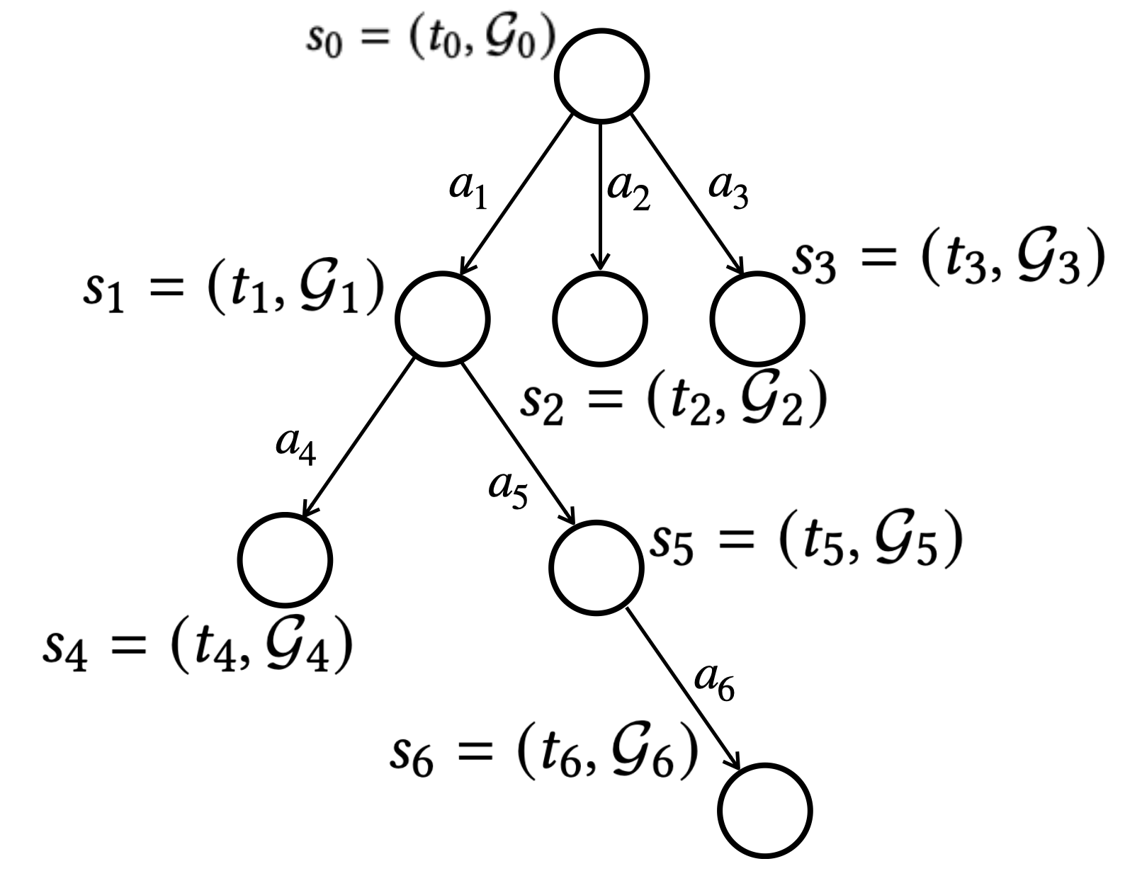
Figure 1: An example of search tree $Tree(s)$.

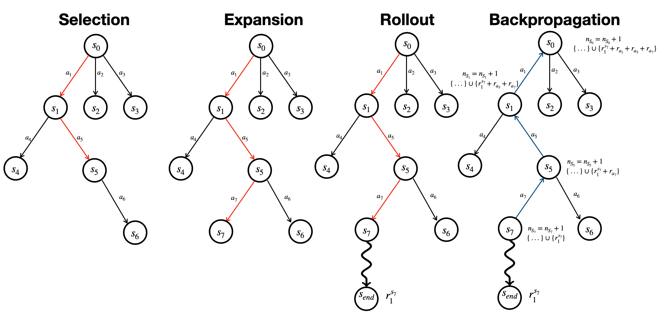
Figure 2: Perform a new simulation on search tree $Tree(s)$ in Fig. 1.

3.3 Monte Carlo Online Planning

Since random events arrive over time, our goal is to build a TEG online in order to adapt to such events, with the aim to maximize collected rewards. Action space $\pazocal A(t,st(t))$ consisting of the possible time-expanded edges that can be added might be too big for Q-learning methods. In such cases, Monte Carlo Tree Search (MCTS) is preferable. MCTS converges to the optimal policy (i.e., the sequence of action which collects the most reward) as the agent collects more and more experience [35, Theorem 6].

MCTS constructs a search tree $\textit{Tree}(s)$, starting from current state $st(t)=(cx(t),\pazocal G(t))$ as root. $\textit{Tree(}s)$ is a decision tree, each node represents a new state resulting from an action. $\textit{Tree}(s)$ is created by running $n$ simulations. In each simulation, a sequence of random events is generated randomly, trying to mimic the statistical characteristics of the environment. Moreover, time advancement is also simulated. Fig. 1 shows an example of $\textit{Tree}(s)$. Each node on the tree is identified by pair $s_{k}=(t_{k},\pazocal G_{k})$.

Suppose we are at time $t$ and we need to take an action, guided by MCTS. To do so, we have to construct a tree via simulation. We set the root as $(t_{0},\pazocal G_{0})$, where $t_{0}=t$ and $\pazocal G_{0}=\pazocal G(t)$. We also consider context $cx_{0}=cx(t)$. We then start a simulation. An action is chosen in $\pazocal A(t_{0},\pazocal G_{0})$, which deterministically induces another node $(t_{1},\pazocal G_{1})$, where $\pazocal G_{1}$ is the graph obtained after the chosen action and $t_{1}$ is the next time instant in which it would be possible to take an action. In the meantime, the reward that would be collected if such an action was really put in place is estimated, based on a simulated sequence of events between $t_{0}$ and $t_{1}$, together with the modifications induced on the context, which would thus go from $cx_{0}$ to $cx_{1}$. We continue the simulation: from node $(t_{1},\pazocal G_{1})$, we choose another action, and we repeat the same reasoning as before, going, for instance, to node $(t_{4},\pazocal G_{4})$ of the tree (Fig. 1). We end the simulation after a certain number of actions (which must be decided as a hyperparameter). We repeat $n$ simulations, similarly.

After those simulations, we can estimate how promising each sequence of actions is. Indeed, we can associate to node $(t_{k},\pazocal G_{k})$ of the tree, number $n_{s_{k}}$ of simulations that have passed through node $(t_{k},\pazocal G_{k})$, and set $\{r^{(t_{k},\pazocal G_{k})}_{1},r^{(t_{k},\pazocal G_{k})}_{2},...,r^{(t_{k},\pazocal G_{k})}_{n_{t_{k},\pazocal G_{k}}}\}$ of cumulative rewards collected in those simulations, counting rewards only starting from $t_{k},\pazocal G_{k}$. We now detail better the aforementioned simulations.

Each simulation includes the following four steps (selection, expansion, rollout, backpropagation). A simulation is a complete path from the root to a leaf in Fig. 1.

Step one: selection. We start from the root $t_{0},\pazocal G_{0}$, and select the child node on the tree with the largest Upper Confidence Bound applied to trees (UCT) [36, Figure 1]. The UCT of node $(t_{k},\pazocal G_{k})$ is:

$$UCT(t_{k},\pazocal G_{k})=\frac{1}{n_{t_{k},\pazocal G_{k}}}\sum_{i=1}^{n_{t_{k},\pazocal G_{k}}}r_{i}^{{t_{k},\pazocal G_{k}}}+c\sqrt{\frac{\ln n_{t_{0},\pazocal G_{0}}}{n_{t_{k},\pazocal G_{k}}}}$$ (1)

where $c$ is a constant, e.g., $c=2$. The selection process ends until that it finds a node which can be expanded. For example, The selection process of Fig. 2 finds the expandable node is node $s_{5}$.

Step two: expansion. The expandable node usually has some actions that have never been selected in previous simulations, so the expansion process will randomly select one of the actions and initialize the child node accordingly. In Fig. 2, action $a_{7}$ has never been selected before, so this time the simulation will first select action $a_{7}$, and then initialize the child node $s_{7}$ with a triple $(s_{7},n_{s_{7}}=0,\emptyset$).

Step three: rollout. After the expansion process, we reach a new leaf node. Starting from this leaf node, we select a sequence of actions uniformly at random, for $N_{\text{end}}$ (hyperparameter) times. At the same time, we record the sum of simulated rewards in rollout process as the cumulative reward starting from the leaf node. For example, in Fig. 2, rollout process starts from leaf node $s_{7}$, after a series of actions, finally reach to the node $s_{end}$. Accumulated reward $r^{s_{7}}_{1}$ in the process is calculated.

Step four: backpropagation. For all nodes passed by the selection process and expansion process, their number of visits will be increased by one, and their new cumulative rewards are recorded. For example, in Fig. 2, node $s_{5}$ is visited. Therefore, we update node $s_{5}$:

$$n_{s_{5}}\leftarrow n_{s_{5}}+1$$ (2)

and

$$\{r^{s_{5}}_{1},r^{s_{5}}_{2},...,r^{s_{5}}_{n_{s_{5}}}\}\leftarrow\{r^{s_{5}}_{1},r^{s_{5}}_{2},...,r^{s_{5}}_{n_{s_{5}}}\}\cup\{r^{s_{7}}_{1}+r_{a_{7}}\}$$ (3)

where reward $r_{a_{7}}$ is the reward of taking action $a_{7}$ in this simulation. Other nodes are updated according to the same method.

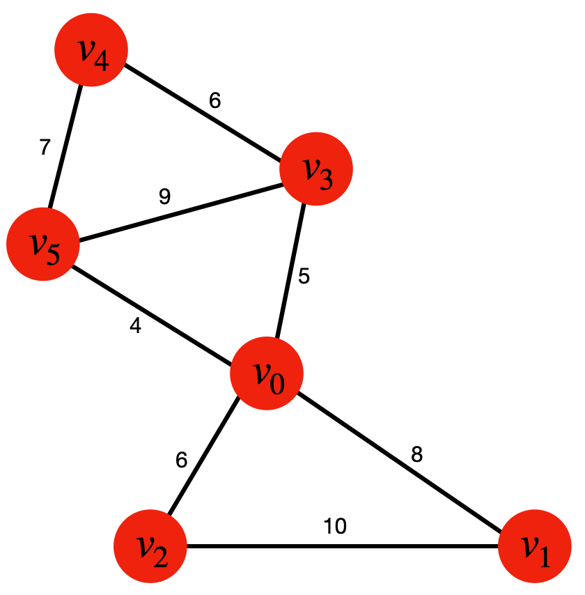
(a) Substrate graph $\pazocal{G}_{\text{substr}}=(\pazocal{V},\pazocal{E}_{\text{substr}})$

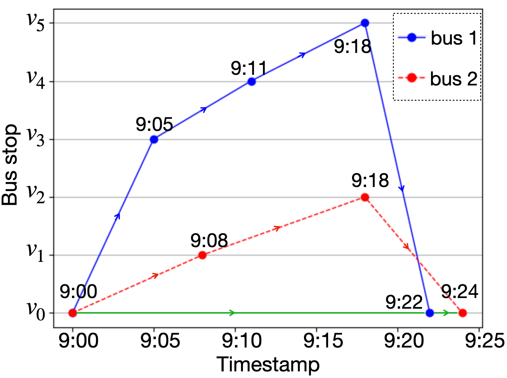
(b) TEG of bus schedule (2 buses)

Figure 3: A toy-example of TEG $\pazocal{G}$ of the bus network.

($\pazocal{G}=(\pazocal{V},\pazocal{E}_{\text{substr}},\pazocal{E})$ where $\pazocal{V}$ and $\pazocal{E}_{\text{substr}}$ are shown in (a), $\pazocal{B}=\{1,2\}$, and $\pazocal{E}$ is shown in (b).)

Suppose, in the real system, we are at time $t$ and state $st(t)=(cx(t),\pazocal G(t))$ and we wish to use MCTS to help us make the next decision. MCTS will start from root node $s_{0}=(t_{0}=t,\pazocal G_{0}=\pazocal G(t))$ and perform the simulations explained above. Note that the actions taken in the simulations have no effect in the real system: the graph in the real system remains $\pazocal G(t)$ although during simulation many other graphs are evaluated. After MCTS finishes, we can apply in the real system the most promising action, which is the one corresponding to a child of the root associated with the highest simulated reward.

Since we do not advance the actual time during the MCTS simulations, we cannot get new events from the real environment Env. Therefore, we need to generate a virtual environment Env’ based on the historical data of environment Env. The events required for the MCTS simulations process all come from this virtual environment Env’.

Algorithm 1 Online Design of Dynamic Networks (OD²N)

1:  Input Substrate graph $\pazocal{G}_{\text{substr}}=(\pazocal{V},\pazocal{E}_{\text{substr}})$                Starting time $t_{0}$.                Ending time $t_{1}$.                Look-ahead buffer $B$.

2:  Initialization

3:  Current time $t=t_{0}$.

4:  Initial context $cx(t)=\emptyset$.

5:  Initial TEG $\pazocal G(t)=(\pazocal{V},\pazocal{E}_{\text{substr}},\pazocal{E}(t)=\emptyset)$.

6:  Initial state $st(t)=(cx(t),\pazocal G(t))$.

7:  Initialize $\pazocal{E}(t)$ by adding random edges (while satisfying system constraints)

8:  repeat

9:     Let real world time $t$ advance.

10:     if Environment Ev generates event $ev$ in $t$ then

11:        Update context $cx(t)$

12:        Collect corresponding reward $r(ev(t),cx(t),\pazocal G(t))$.

13:     end if

14:     if Time instant $t$ is an action instant (§3.2) then

15:        Evaluate available actions $\pazocal A(t,s(t))$, which consist of adding time-expanded edges with departure later than $t+B$.

16:        Choose action $a(t)\in\pazocal A(t,s(t)))$ by running MCTS (§ 3.3).

17:        Apply action $a(t)$, i.e., add the corresponding edge to $\pazocal G(t)$.

18:        Evaluate reward $r(a(t),cx(t),\pazocal G(t))$ obtained via action $a(t)$.

19:     end if

20:  until $t>t_{1}$.

21:  Return contexts $cx(t)$ or data required for different problems.

3.4 Online Design of Dynamic Networks (OD²N) Algorithm

We propose Algorithm 1 to design the reactive networks. Our basic idea is to use MCTS introduced in Section 3.3 to choose actions, then update the state of the network based on these actions, and record changes during state transitions. It should be noted that Algorithm 1 is an online method, and we can set ending time $t_{1}=\infty$, which means that we will never terminate the algorithm to provide network designing plans in real time.

3.5 Application to Configuration of Complex Systems

Before delving into our main application (§4), we provide here briefly some high-level thoughts on how our method could be applied for deciding switching among configurations of a complex system [25]. In this case, substrate graph $\pazocal{G}_{\text{substr}}=(\pazocal{V},\pazocal{E}_{\text{substr}})$ consists of sets $\pazocal{V}$ of potential configurations and $\pazocal{E}_{\text{substr}}\subseteq\pazocal{V}\times\pazocal{V}$ of edges. An edge represents the possibility to switch between two configurations. When we decide on an action, which is to switch configurations, the environment Env gives us a certain cost suffered from the system (opposite of reward $r$), which depends on its current configuration. Contest $cx(t)$ is the accumulated cost up to $t$. Having defined states, actions and reward, we can use our method to design the evolution of configuration switches of the complex system, in real time, with the aim to minimize accumulated stochastic cost.

4 Specialization of the method for the Online Bus Network Design

We now apply our general framework to design a futuristic public transport system, in which a network of bus lines is designed online and dynamically evolves, to adapt to a stochastic sequence of user trip requests. This problem can be also framed as a Dynamic Vehicle Routing Problem (DVRP), where incoming requests are associated to vehicles, whose routes are adjusted on the fly. DVRP is a solution to route a fleet of shared taxis for low density demand, whose vehicle routes are extended independently. We tackle instead a system comparable with conventional public transport, which can achieve similar high capacity via building a structured network of bus lines, where transfers are possible. The difference with conventional public transport is that bus lines evolve over time.

4.1 Time-Expanded Graph of a Bus Network

In the case considered here, substrate graph $\pazocal{G}_{\text{substr}}=(\pazocal{V},\pazocal{E}_{\text{substr}})$ consists of sets $\pazocal{V}$ of potential bus stops and $\pazocal{E}_{\text{substr}}\subseteq\pazocal{V}\times\pazocal{V}$ of edges (Fig. 3-(a)). Edge $(v,v^{\prime})\in\pazocal{E}_{\text{substr}}$ indicates that a bus can travel directly from stop $v$ to stop $v^{\prime}$, taking time $w_{v,v^{\prime}}$. We further introduce a set $\pazocal{B}$ of $N$ buses.

A Time-Expanded Graph (TEG) is a tuple $\pazocal{G}(t)=(\pazocal{V},\pazocal{E}_{\text{substr}},\pazocal{E}(t))$ in our case. Set $\pazocal{E}(t)$ contains all the possible transitions that users can choose before time $t+B$. To be more precise, time-expanded edge $e=(v,v^{\prime},t)\in\pazocal{E}(t)$ means the following: if $v^{\prime}\neq v$, edge $e$ represents that there is a bus departing from bus stop $v$ to bus stop $v^{\prime}$ at time $t$ (red lines and blues lines in Fig. 3 (b)); if $v^{\prime}=v$, edge $e$ represents that a user begin to wait in a bus stop $v$ at time $t$ until a bus arrives (green lines in Fig. 3 (b)). For example, in Fig. 3 (b), when we schedule that bus $1$ to arrive at stop $v_{0}$ at 9:22 and bus $2$ to arrive at $v_{0}$ at 9:24, we automatically add an edge (green line) from (9:22,$v_{0}$) to (9:24,$v_{0}$), which allows users us to transfer from bus $1$ to bus $2$, waiting for $2$ minutes.

An Event $ev(t)$ is a request $d=(v,v^{\prime},t)$, where $v,v^{\prime}\in\pazocal{V}$ are the origin and destination nodes respectively, $t$ is the departure time of a passenger. Routing request $d$ into TEG $\pazocal G(t)$ means to calculate a time-expanded path, defined as $p=(v,t,e_{1},\dots,e_{n},v^{\prime})$, where $e_{1},\dots,e_{n}$ is a set of time-expanded edges in $\pazocal G(t)$. Path $p$ must satisfy the following conditions:

$$t+w_{v,v_{1}} \leq t_{1}$$ (4)

$$e_{j} =(v_{j},v_{j+1},t_{j})\in\pazocal{E}, \forall j=1,\dots,n$$ (5)

$$t_{j}+w_{v_{j},v_{j+1}} \leq t_{j+1}, \forall j=1,\dots,n-1$$ (6)

$$v_{1}=v, \,\,\,\ v_{n+1}=v^{\prime}$$ (7)

The arrival time of $p$ is $t^{\prime}(p)=t_{n}^{\prime}+w_{v_{n}^{\prime},v^{\prime}}$. Let $\pazocal{P}(v,v^{\prime},t,\pazocal{G})$ be the set of paths in $\pazocal{G}$ starting at node $v\in\pazocal{V}$ at time $t$ and arriving at node $v^{\prime}\in\pazocal{V}$. The shortest path is $p^{*}(v,v^{\prime},t)\in\arg\min_{p\in\pazocal{P}(v,v^{\prime},t,\pazocal{G})}t_{p}^{\prime}.$

We associate to request $d=(v,v^{\prime},t)$ the shortest path $p^{*}(d)=p^{*}(v,v^{\prime},t)$. TEG $\pazocal G(t)$ is composed of a set of time-expanded subgraphs, each representing the movement of a bus. Time-expanded subgraph $\pazocal{SG}_{i}(t)$ of bus $i\in\pazocal B$ is composed of a sequence of edges, describing its movement. Designing a bus network amounts to design such subgraphs, by taking actions, consisting in adding time-expanded edges to each subgraph, over time. Such time-expanded subgraphs are however not extended in isolation, as the quality of a sequence of actions is measured against the user requests served collectively by the entire network. Differently from the classic DVRP approach, a vehicle route is not modified in order to accommodate one request in particular. Each modification is aimed at making the entire graph more capable of serving future requests, by creating relevant connections between time-expanded subgraphs that allow transfers.

4.2 Online bus network design process

We here adapt our generic decision process (§3.2) to the online bus network design task. Let $t$ denote the current real-world time and $\pazocal G(t)$ the TEG available at time $t$. All edges departing before $t+B$ must be already present in $\pazocal G(t)$. In other words, the schedule in the interval $[t,t+B]$ of all buses has been already planned at time $t$ and is modeled by $\pazocal G(t)$. Environment Env is in this case a process that generates user requests. Context $cx(t)$ is the list of requests not yet served at time $t$. The state is $st(t)=(cx(t),\pazocal G(t))$. Considering a request $d$ that arrives at $t$, or is in list $cx(t)$, it is served if there exists a path (and thus shortest path $p^{*}(d)$) inside TEG $\pazocal G(t)$.

For bus $i\in\pazocal B$, let $e_{i}^{\text{last}}(t)=(v,v^{\prime},t^{\prime})$ the last edge, i.e., the edge of subgraph $\pazocal{SG}_{i}$ with the latest departure time. Let $\tau_{i}(t)$ the arrival time of such an edge. Observe that, by construction, $\tau_{i}(t)\geq t+B$. Bus $i^{*}(t)=\arg\min_{i\in\pazocal B}\tau_{i}(t)$ is thus the bus whose line requires to be extended before the others. If $\arg\min_{i\in\pazocal B}\tau_{i}(t)$ does not return a single bus, we break ties choosing $i^{*}(t)$ randomly among them. Observe also that at real-world time $t$, the entire schedule of the bus lines is already planned in interval $[t,\tau_{i^{*}(t)}(t)]$ and will never be changed. At current real-world time $t$, if $\tau_{i^{*}(t)}>t+B$, we do nothing and let real world time $t$ advance until $\tau_{i^{*}}(t)=t+B$, which we set as action instant. At this moment, we take an action. As introduced in the generic description in Sec. 3.2, this is an example of action instants being determined by the state in which we are (in this case, in particular, it is the last edge of bus $i^{*}(t)$ that determine the action instant).

An action $a(t)\in\pazocal A(t,st(t))$ available at time $t$ consists in extending $\pazocal{SG}_{i^{*}(t)}$ by adding a time-expanded edge $e_{a(t)}=(v^{\prime},v^{\prime\prime},t+B)$, where $v^{\prime}$ is the arriving stop of the last edge of bus $i$. After action $a(t)\in\pazocal A(t,st(t))$ is taken, and the subgraph of bus $i^{*}(t)$ expanded, we let the real world time advance and we repeat the process. In order to select which of the actions available in $\pazocal A(t,st(t))$ should be taken, we ran MCTS, as explained in §3.3.

In parallel, new requests arrive. If request $d$ arrives at time $t$, we check immediately if it can be served (see first paragraph of this subsection). If yes, we increase the collected reward by $1$. If not, the request is put in the unserved request list $cx(t)$. Every time instant $t$ in which we take an action, we check if some of the unserved requests in $cx(t)$ can be served with the new expanded graph. If yes, we increase the reward accordingly and remove those requests from $cx(t)$.

4.3 Requests Generation Model

As explained in §3.3, MCTS simulates future possible evolution trajectories of the system, so that one can choose the next action that will likely induce the most desirable evolution. To perform such simulation, we need a model Env’ of the environment, which generates events (requests in this case) that are statistically similar to those generated by the real environment Env. We can build from historical data of real-world environment Env. In the transport case we are tackling here, model $\textit{Env}^{\prime}$ can be trained on historical dataset $\pazocal D$ of previously observed trips. Requests are a spatial-temporal marked point process [37]. Therefore, $\textit{Env}^{\prime}$ must be able to mimic the spatial patterns (where origins and destinations of trips are distributed) and temporal patterns (rate of requests).

1. Learning temporal patterns. For each day in the past, we first count the number of requests generated at different timeslots. We train a support-vector machine (SVM) so that it predicts sufficiently well the request counts of all timeslots in the next day.

2. Learning spatial patterns. We count the origin and destination of all past requests and build an OD matrix $M=\{a_{uv}\}_{u,v\in\pazocal V}$ where $a_{uv}$ is the fraction of observed trips that went from origin $u$ to destination $v$. The value of $a_{ij}$ can be interpreted as the probability that, given any trip request, its origin will be $u$ and its destination $v$.

When, within MCTS, we use $\textit{Env}^{\prime}$ to generate simulated requests, we do as follows. We first predict the number of future requests via the SVM at each timeslot. For each of them, we randomly select the origin and the destination based on probabilities $a_{u,v}$. Note that, instead of this very simple $\textit{Env}^{\prime}$, one may pick any of the advanced demand prediction models available in the literature, which is however outside the scope of this work.

5 Experimental Results

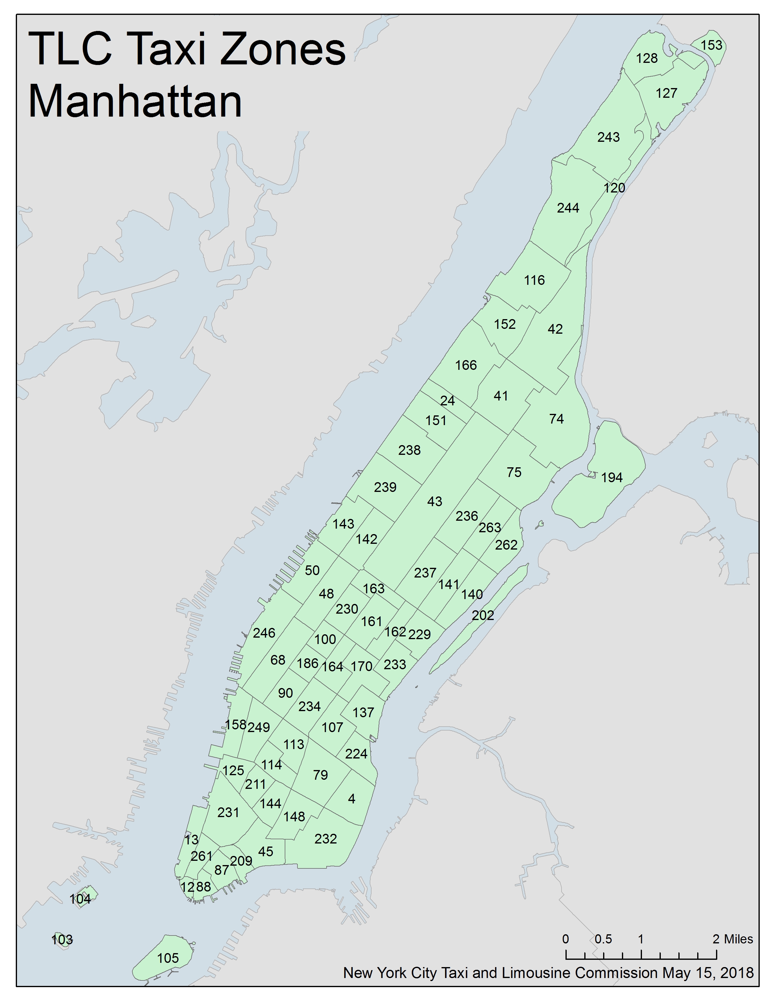
Figure 4: Taxi zones in Manhattan.

5.1 Considered scenario

We apply our method to design a bus network online in a scenario in Manhattan (Table 1), where the environment consists of a sequence of trip requests from end-users. To test our method, we replay a randomly selected subset of real taxi requests from a public dataset [38]. Taxi zones are shown in Fig. 4. Manhattan has 67 taxis zones. We find the centroid of each taxi zone, and use these centroids as candidate bus stops. In this case, substrate graph $\pazocal{G}_{\text{substr}}=(\pazocal{V},\pazocal{E}_{\text{substr}})$, where $\pazocal{V}$ is the set of all centroids. Graph $\pazocal{G}_{\text{substr}}$ is a fully connected graph. Weight $w_{u,v}$ of edge $(u,v)\in\pazocal{G}_{\text{substr}}$ is the time (in minutes) to travel between nodes, i.e., $w_{u,v}=d(u,v)/v_{\text{bus}}$, where $d_{u,v}$ is the distance between $u,v\in\pazocal V$ and $v_{\text{bus}}$ is the average speed of the bus. We introduce set $\pazocal{B}$ of $N$ buses, with random initial positions.

Table 1: Scenario parameters

Parameter	Value
Number of candidate bus stops	67
Fleet size $N$	5, 10, 20, 30, 40, 50
Speed of a bus $v_{\text{bus}}$	17.3 km/h [39]
Speed of a private car $v_{\text{car}}$	11.4 km/h [39]
Walking speed $v_{\text{walk}}$	4.3 km/h [40]
Rollout termination number $N_{end}$	5
Look-ahead buffer $B$ of Algorithm 1	30 mins
Timeslot for training model $\textit{Env}^{\prime}$ (§4.3)	1 minute
Training set $\pazocal{D}$ (§4.3)	All request data from [38]
	in February 2024
Tested scenario (§4.3)	20% of request data from [38]
	(to get faster results)
	March 1, 2024, 9:00-13:00

5.2 Performance

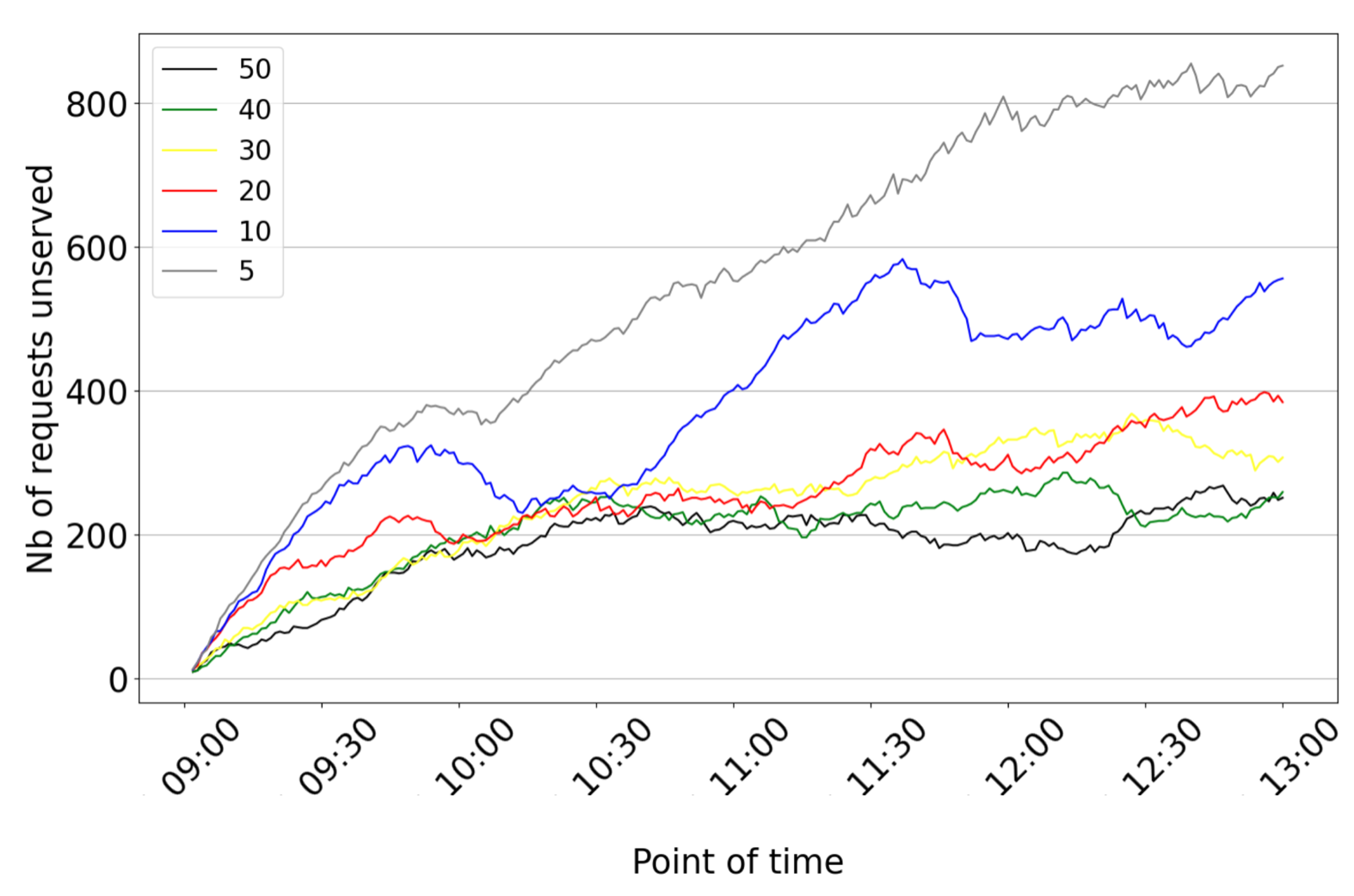
(a) Number of unserved requests.

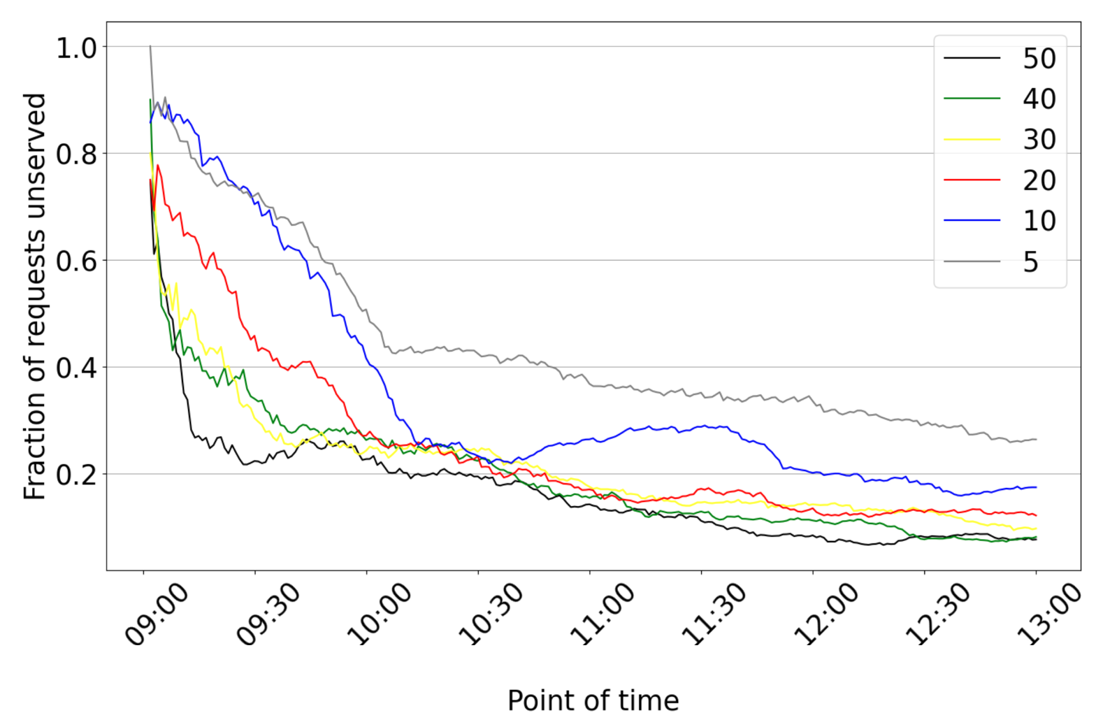
(b) Fraction of requests unserved.

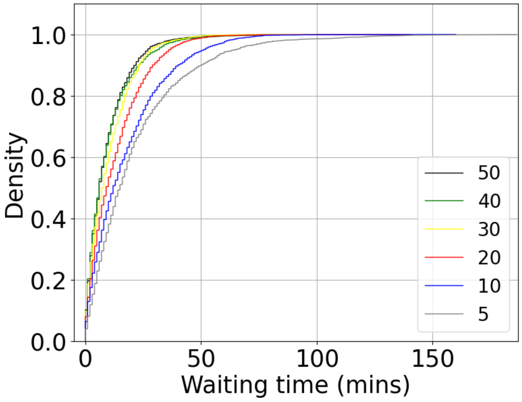
(c) ECDF of the waiting time.

Figure 5: Real-time MCTS results with different fleet sizes from 9:00 to 13:00.

Upon arrival, a request is placed in a list of unserved requests. Figure 5-(a) shows the number of such requests over time. For any fleet size, the number of unserved requests increased significantly in the period starting at 9:00. This is because our system has just started, and at $t=$9:00 we initialize TEG $\pazocal G(t)$ randomly (Alg. 1), which means that bus schedule is randomly planned in until time $t+B=9:30$. After the simulation runs for a period of time, the real-time number of unserved requests no longer increases significantly. Figure 5 (b) shows the percentage of unserved requests out of all requests received so far. Unserved requests go below 8% with a sufficiently large fleet size. It should be noted that, in any dynamic bus system, it is impossible to serve all requests. There can be requests whose origin and destination are very far or in remote places. This kind of trips might be rejected also in current real transport system (and the user would be better-off taking their car). Public transport needs indeed to balance user satisfaction and efficiency, and it cannot thus provide a service tightly tailored to very specific user needs. Differently from [32], which sets a maximum waiting time after which users are rejected, we count all unserved requests in Fig. 5, no matter their waiting time.

Table 2: Comparison with SOTA (40 buses)

	SOTA (Max. waiting time 20 mins)	SOTA (Max. waiting time 30 mins)	Our method (Max. waiting time 20 mins)	Our method (Max. waiting time 30 mins)
Service rate	34.37%	49.70%	84.01%	90.66 %
Average Waiting time (mins)	4.16	4.73	6.49	7.93

In Table 2, we instead test two values of maximum waiting time and compare our results with an algorithm [32] largely known as state-of-the-art (SOTA), of which we run an open source implementation [41]. We run both algorithms with a fleet size of 40 and infinite seat capacity. We wish indeed to first evaluate the level of sharing the system can obtain and choose the appropriate seat capacity a-posteriori. Observe that the goal of SOTA is to optimize an on-demand “high-capacity” ride-sharing, in which the route of each vehicle is adjusted independently, by adding some new requests as they come. In such a system, vehicle routes are not structured and users cannot perform transfers from a vehicle to another. Our method allows instead to run a public transport system that does not exist yet, which is dynamic, as ride-sharing, but at the same time builds a structured network of bus lines, where transfers from a line to another are enabled. In this sense, our system is similar to conventional public transport, and offers much more capacity (higher service rate) than SOTA ride-sharing. The difference with respect to conventional public transport is that the network of lines evolves over time. As expected, higher capacity is achieved by increasing waiting times, but this increase is however under a completely acceptable level (Table 2). Consider also that, in case a user transfers over multiple lines, the waiting time to board all these lines is recorded, and the sum is presented in Table 2.

Table 3: Comparison of results with different fleet sizes

Fleet size	Average occupation	Average Waiting time	Average in-vehicle time	Average stretch (taxi)	Average stretch (walking)	Average number of transfers
5	27.49	21.57	13.90	1.80	0.68	1.24
10	16.64	17.22	15.18	1.56	0.61	1.79
20	10.44	12.86	18.18	1.90	0.72	1.85
30	8.15	10.20	20.65	2.35	0.89	1.59
40	6.68	9.57	22.03	2.62	0.99	1.68
50	6.00	9.11	23.91	2.83	1.07	1.50

Table 3 further shows the difference in performance of our method with different fleet sizes. The average occupation of a bus is computed in the appendix A. The stretch is defined as $\frac{t_{\text{in-vehicle}}\cdot v_{\text{car or walking}}}{O-D\,\text{distance}}$. It is interesting to note that our method adapts to a small fleet, as it is able to increase the level of sharing, i.e., more users share a bus trip. As fleet sizes increases, the average occupation decreases, which suggests that the kind of vehicles that should be adopted might change (from large buses to minibuses). As expected, a larger fleet size reduces waiting time (Table 3 and Fig. 5 (c)), but after a certain fleet size (30 buses), we already achieve good performance (60% of trips have a waiting time within 10 minutes).

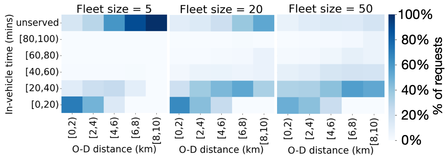
Figure 6: Fraction of requests served with a certain in-vehicle time over total requests, per each O-D distance interval.

In Figure 6 we study how our system serves trips of different length. We divide both O-D distance and in-vehicle time into five intervals. For each O-D distance interval, we count how many requests were issued by users, and we then calculate the fraction of such requests served with an in-vehicle time between 0 and 20 minutes, between 20 and 40 minutes, etc. The color scale indicates such fraction. for example, the bottom left square color represents

$$\frac{\text{served requests with OD dist.}\in[0,2\text{km})\text{ and in-veh trav.time}\in[0,20\text{min})}{\text{All requests issued with O-D distance}\in\,[0,2\text{km})}.$$

Fig. 6 shows that more trips are served with higher fleet size, in particular “long” trips (high O-D distance), which are all unserved with 5 buses. Unserved long trips might require paths longer than $B=$30 minutes (which is the maximum path allowed into the system), and might be served with higher look-ahead buffer $B$.

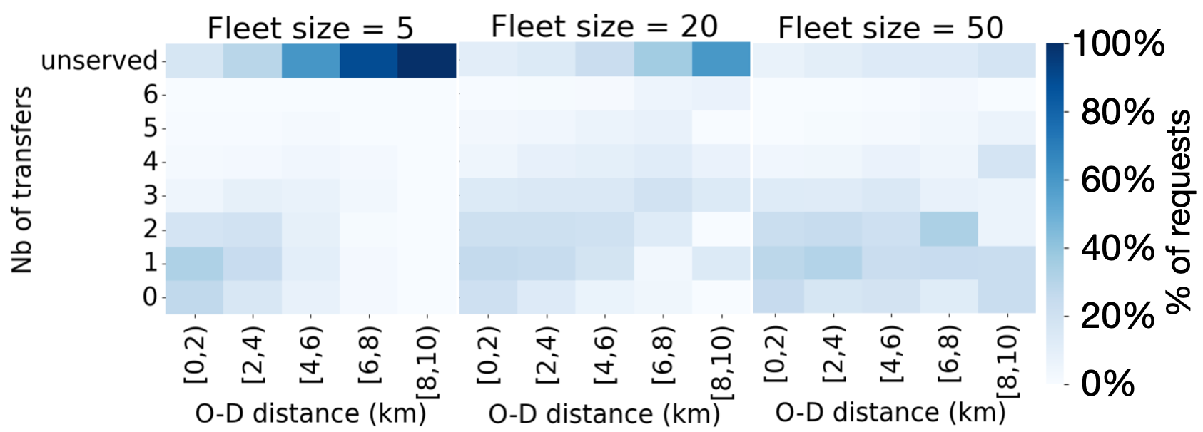
Figure 7: Fraction of requests experiencing certain number of transfers over total requests, per each O-D distance interval.

Figure 7 represents the number of transfers per trip and is obtained in the same way as Figure 6. We observe that, with a larger fleet size, more transfers are possible, as the network of bus lines is denser. In a real system, it would be reasonable to limit the number of transfers, which negatively impact user experience. We could easily adapt our MCTS approach to the case in which users accept to do at most 1 or 2 transfers: it would suffice to consider as “served” users that can go from origin to destination with no more than those transfers and keep in the “unserved” list all the other users. In this way, the MCTS algorithm would collect rewards only for the trips respecting the “maximum transfers constraint” and would learn to adjust bus lines accordingly.

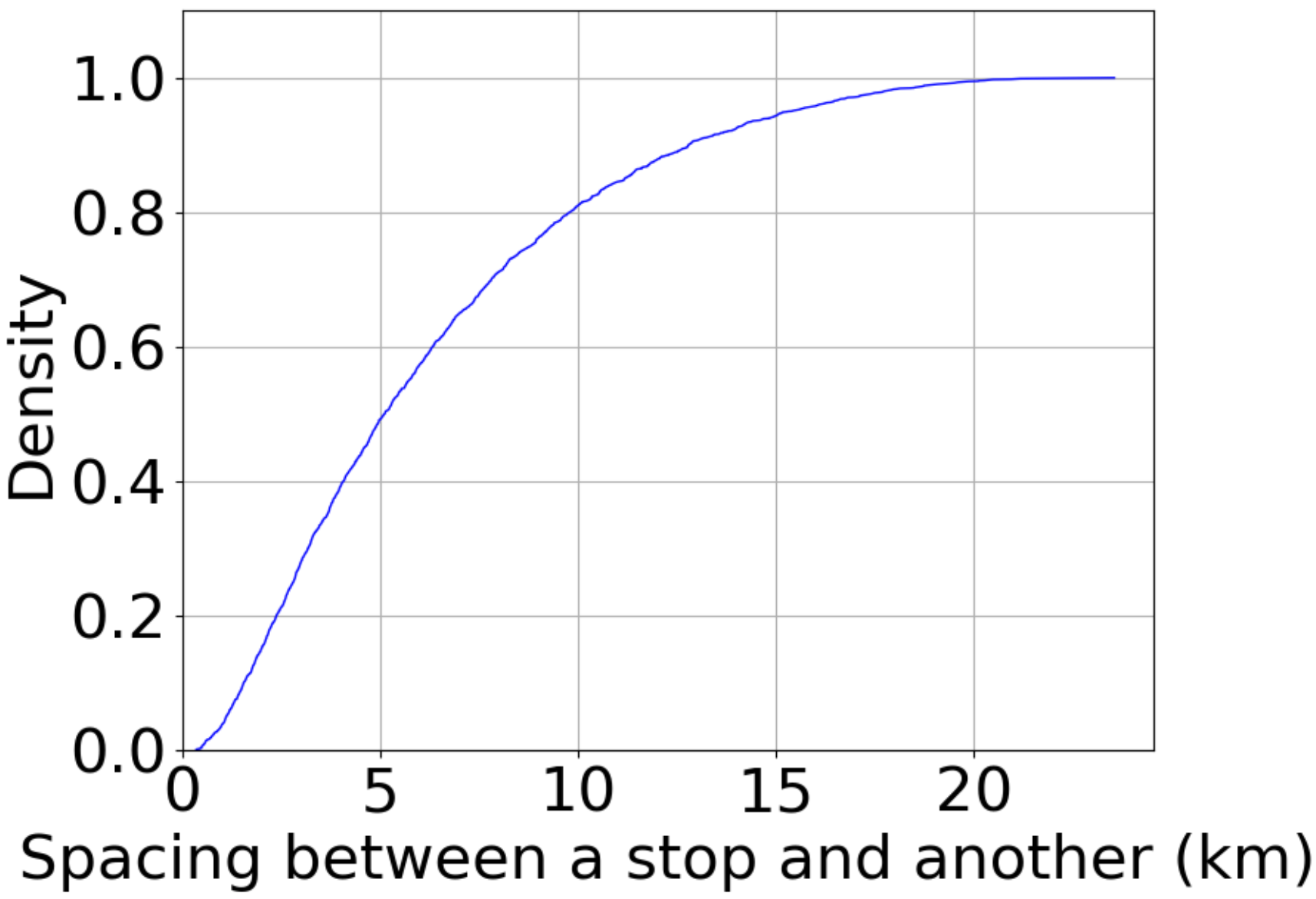
Figure 8: ECDF of the spacing between a stop and another.

Finally, Fig. 8 shows that the distance between two consecutive stops served by a bus is higher than in conventional bus services. Our service thus resembles an express service. This is coherent with the observation that humanly designed stop spacing of real bus services is too large and inefficient [42].

6 Conclusion

In this paper, we introduced the novel problem of designing temporal graphs. Our framework allows building networks able to react to a stochastic environment and adjust their evolution in order to keep satisfying performance. We formalized a general rolling horizon decision process and a Monte Carlo Tree Search-based solution method. We showcased the potential of our approach in a transport context, by designing a futuristic fully dynamic network of bus lines that is able to adapt to a stochastic and unknown request arrival. Our designed network outperforms state-of-the-art Dynamic Vehicle Routing Problem (DVRP) algorithms. This work opens new research avenues on the design of dynamic networks, whose application can go far beyond the transport context showcased here.

Appendix A Average occupation of a bus

We measure the average in-vehicle time $t_{\text{in-vehicle}}$, total number of served request $N_{\text{served}}$ and the considered time interval $t_{\text{simulation}}=t_{1}-t_{0}$. We also know fleet size $N$. The Average occupation of a bus is:

$$N_{\text{occupation}}=\frac{N_{\text{served}}}{N\cdot t_{\text{simulation}}}\cdot t_{\text{in-vehicle}}.$$

Factor $\frac{N_{\text{served}}}{t_{\text{simulation}}}$ represents the rate of requests (req/min) the system is supposed to pickup. The average rate of requests picked up by one bus is thus $\frac{N_{\text{served}}}{N\cdot t_{\text{simulation}}}$. Requests $\frac{N_{\text{served}}}{N\cdot t_{\text{simulation}}}$ picked up at $t$ will leave at $t+t_{\text{in-vehicle}}$ on average, but the bus can also pick up the same number $\frac{N_{\text{served}}}{N\cdot t_{\text{simulation}}}$ of requests at $t+t_{\text{in-vehicle}}$ on average. If a bus starts running at time $t_{0}$, during this time interval [$t_{0}$,$t_{0}+t_{\text{in-vehicle}}$], a bus can generally pick up $\frac{N_{\text{served}}}{N\cdot t_{\text{simulation}}}\cdot t_{\text{in-vehicle}}$ requests, and after $t_{0}+t_{\text{in-vehicle}}$, the number of pickup requests and dropoff requests is equal on average, so the occupation of the bus will remain the same on average.

References

- [1] Feng Xia, Ke Sun, Shuo Yu, Abdul Aziz, Liangtian Wan, Shirui Pan, and Huan Liu. Graph learning: A survey. IEEE Transactions on Artificial Intelligence, 2(2):109–127, 2021.
- [2] Ziwei Zhang, Peng Cui, and Wenwu Zhu. Deep learning on graphs: A survey. IEEE Transactions on Knowledge and Data Engineering, 34(1):249–270, 2020.
- [3] Bing Yu, Haoteng Yin, and Zhanxing Zhu. Spatio-temporal graph convolutional networks: A deep learning framework for traffic forecasting. arXiv preprint arXiv:1709.04875, 2017.
- [4] Weiwei Jiang and Jiayun Luo. Graph neural network for traffic forecasting: A survey. Expert Systems with Applications, 207:117921, 2022.
- [5] Songgaojun Deng, Huzefa Rangwala, and Yue Ning. Learning dynamic context graphs for predicting social events. In Proceedings of the 25th ACM SIGKDD International Conference on Knowledge Discovery & Data Mining, pages 1007–1016, 2019.
- [6] Chen Gao, Xiang Wang, Xiangnan He, and Yong Li. Graph neural networks for recommender system. In Proceedings of the Fifteenth ACM International Conference on Web Search and Data Mining, pages 1623–1625, 2022.
- [7] Giovanni Mauro, Massimiliano Luca, Antonio Longa, Bruno Lepri, and Luca Pappalardo. Generating mobility networks with generative adversarial networks. EPJ data science, 11(1):58, 2022.
- [8] Antonio Longa, Giulia Cencetti, Bruno Lepri, and Andrea Passerini. An efficient procedure for mining egocentric temporal motifs. Data Mining and Knowledge Discovery, 36(1):355–378, 2022.
- [9] Mike KP So, Agnes Tiwari, Amanda MY Chu, Jenny TY Tsang, and Jacky NL Chan. Visualizing covid-19 pandemic risk through network connectedness. International Journal of Infectious Diseases, 96:558–561, 2020.
- [10] xxx. Our repository: the url will be provided after acceptance, to comply to double-blind policy. xxxxx, 2025.
- [11] Philippe Fournier-Viger, Ganghuan He, Chao Cheng, Jiaxuan Li, Min Zhou, Jerry Chun-Wei Lin, and Unil Yun. A survey of pattern mining in dynamic graphs. Wiley Interdisciplinary Reviews: Data Mining and Knowledge Discovery, 10(6):e1372, 2020.
- [12] Jinghan Meng and Yi-cheng Tu. Flexible and feasible support measures for mining frequent patterns in large labeled graphs. In Proceedings of the 2017 ACM International Conference on Management of Data, pages 391–402, 2017.
- [13] Mathias Fiedler and Christian Borgelt. Support computation for mining frequent subgraphs in a single graph. In MLG, 2007.
- [14] Sajal Halder, Md Samiullah, and Young-Koo Lee. Supergraph based periodic pattern mining in dynamic social networks. Expert Systems with Applications, 72:430–442, 2017.
- [15] Michele Berlingerio, Francesco Bonchi, Björn Bringmann, and Aristides Gionis. Mining graph evolution rules. In Machine Learning and Knowledge Discovery in Databases: European Conference, ECML PKDD 2009, Bled, Slovenia, September 7-11, 2009, Proceedings, Part I 20, pages 115–130. Springer, 2009.
- [16] Ruoming Jin, Scott McCallen, and Eivind Almaas. Trend motif: A graph mining approach for analysis of dynamic complex networks. In Seventh IEEE International Conference on Data Mining (ICDM 2007), pages 541–546. IEEE, 2007.
- [17] Aravind Sankar, Yanhong Wu, Liang Gou, Wei Zhang, and Hao Yang. Dysat: Deep neural representation learning on dynamic graphs via self-attention networks. In Proceedings of the 13th international conference on web search and data mining, pages 519–527, 2020.
- [18] Alireza Shams Shafigh, Beatriz Lorenzo, Savo Glisic, Jordi Pérez-Romero, Luiz A DaSilva, Allen B MacKenzie, and Juha Röning. A framework for dynamic network architecture and topology optimization. IEEE/ACM Transactions on Networking, 24(2):717–730, 2015.
- [19] Saghar Hosseini, Airlie Chapman, and Mehran Mesbahi. Online distributed convex optimization on dynamic networks. IEEE Transactions on Automatic Control, 61(11):3545–3550, 2016.
- [20] Purnamrita Sarkar, Deepayan Chakrabarti, and Michael Jordan. Nonparametric link prediction in dynamic networks. arXiv preprint arXiv:1206.6394, 2012.
- [21] Xiaoyi Li, Nan Du, Hui Li, Kang Li, Jing Gao, and Aidong Zhang. A deep learning approach to link prediction in dynamic networks. In Proceedings of the 2014 SIAM international conference on data mining, pages 289–297. SIAM, 2014.
- [22] Akif Rehman, Masab Ahmad, and Omer Khan. Exploring accelerator and parallel graph algorithmic choices for temporal graphs. In Proceedings of the Eleventh International Workshop on Programming Models and Applications for Multicores and Manycores, pages 1–10, 2020.
- [23] Frank Fischer and Christoph Helmberg. Dynamic graph generation for the shortest path problem in time expanded networks. Mathematical Programming, 143(1-2):257–297, 2014.
- [24] Simon Belieres, Mike Hewitt, Nicolas Jozefowiez, Frédéric Semet, and Tom Van Woensel. A benders decomposition-based approach for logistics service network design. European Journal of Operational Research, 286(2):523–537, 2020.
- [25] Matthew R Silver and Olivier L De Weck. Time-expanded decision networks: A framework for designing evolvable complex systems. Systems Engineering, 10(2):167–188, 2007.
- [26] Ido Orenstein and Tal Raviv. Parcel delivery using the hyperconnected service network. Transportation Research Part E: Logistics and Transportation Review, 161:102716, 2022.
- [27] Victor Pillac, Michel Gendreau, Christelle Guéret, and Andrés L Medaglia. A review of dynamic vehicle routing problems. European Journal of Operational Research, 225(1):1–11, 2013.
- [28] Brenner Humberto Ojeda Rios, Eduardo C Xavier, Flávio K Miyazawa, Pedro Amorim, Eduardo Curcio, and Maria João Santos. Recent dynamic vehicle routing problems: A survey. Computers & Industrial Engineering, 160:107604, 2021.
- [29] Marlin Ulmer. Delivery deadlines in same-day delivery. Logistics Research, 10(3):1–15, 2017.
- [30] Marlin W Ulmer. Anticipation versus reactive reoptimization for dynamic vehicle routing with stochastic requests. Networks, 73(3):277–291, 2019.
- [31] Warren B Powell, Hugo P Simao, and Belgacem Bouzaiene-Ayari. Approximate dynamic programming in transportation and logistics: a unified framework. EURO Journal on Transportation and Logistics, 1(3):237–284, 2012.
- [32] Javier Alonso-Mora, Samitha Samaranayake, Alex Wallar, Emilio Frazzoli, and Daniela Rus. On-demand high-capacity ride-sharing via dynamic trip-vehicle assignment. Proceedings of the National Academy of Sciences, 114(3):462–467, 2017.
- [33] Martin Jacobsen and Joseph Gani. Point process theory and applications: marked point and piecewise deterministic processes. 2006.
- [34] Melike Baykal-Gürsoy and K Gürsoy. Semi-markov decision processes. Wiley Encyclopedia of Operations Research and Management Sciences, 10:9780470400531, 2010.
- [35] Levente Kocsis and Csaba Szepesvári. Bandit based monte-carlo planning. In European conference on machine learning, pages 282–293. Springer, 2006.
- [36] Peter Auer, Nicolo Cesa-Bianchi, and Paul Fischer. Finite-time analysis of the multiarmed bandit problem. Machine learning, 47:235–256, 2002.
- [37] Mark S Handcock and James R Wallis. An approach to statistical spatial-temporal modeling of meteorological fields. Journal of the American Statistical Association, 89(426):368–378, 1994.
- [38] Tlc trip record data. https://www.nyc.gov/site/tlc/about/tlc-trip-record-data.page. Accessed: 2024.
- [39] New york city mobility report. https://www.nyc.gov/html/dot/downloads/pdf/mobility-report-2018-screen-optimized.pdf. Accessed: 2018.
- [40] Google map. https://www.google.com/maps. Accessed: 2024.
- [41] MetaZuo. Ride sharing. https://github.com/MetaZuo/RideSharing, 2017.
- [42] Peter G Furth and Adam B Rahbee. Optimal bus stop spacing through dynamic programming and geographic modeling. Transportation Research Record, 1731(1):15–22, 2000.