Domain decomposition for entropic unbalanced optimal transport
Abstract
Solving large scale entropic optimal transport problems with the Sinkhorn algorithm remains challenging, and domain decomposition has been shown to be an efficient strategy for problems on large grids. Unbalanced optimal transport is a versatile variant of the balanced transport problem and its entropic regularization can be solved with an adapted Sinkhorn algorithm. However, it is a priori unclear how to apply domain decomposition to unbalanced problems since the independence of the cell problems is lost. In this article we show how this difficulty can be overcome at a theoretical and practical level and demonstrate with experiments that domain decomposition is also viable and efficient on large unbalanced entropic transport problems.
1 Introduction
1.1 Motivation
(Computational) optimal transport
Optimal transport (OT) is concerned with finding the most cost-efficient way of transforming one probability measure into another. For a measurable cost function and two probability measures and on and the Kantorovich OT problem is given by
| (1) |
where denotes the set of couplings between and , and denotes integration of measurable functions against measures. Thorough introductions to the topic can be found in [16] and [15].
An overview on computational methods can be found in [14]. A common variant of (1) is the addition of entropic regularization:
| (2) |
where is the Kullback-Leibler diveregence and is a positive regularization parameter. This modification has several theoretical and computational advantages with respect to (1). For instance, the optimization problem becomes strictly convex, the optimal value becomes differentiable with respect to the marginals , and (2) can be solved with the Sinkhorn algorithm, which is simple and apt for GPU implementation, see [8, 9, 14] and references therein.
Unbalanced optimal transport
One limitation of problems (1) and (2) is that they can only be applied to positive measures and of equal mass, and that they can be quite susceptible to additive noise. As a remedy, a general framework for unbalanced optimal transport between measures of (possibly) different mass has been proposed, see for instance [10, 7, 12] and references therein. In [12] the constraint that the marginals of must be exactly equal to and is relaxed through entropy functions (also known as divergence functionals) that penalize the deviations from and . The general form of the unbalanced optimal transport (UOT) problem becomes
| (3) |
where and are convex functionals satisfying some properties to be specified in Section 2. It is natural to also consider the entropy regularized variant of (3):
| (4) |
and it is shown in [6] that such problems can be solved with a generalized version of the Sinkhorn algorithm, which preserves its favorable computational properties.
Domain decomposition for optimal transport
Despite its general efficiency, the Sinkhorn algorithm struggles to solve large problems with high precision. One way to address this is domain decomposition [5], originally proposed for unregularized optimal transport in [2]. The strategy of the algorithm is as follows: Let and be two partitions of , and let be an initial feasible coupling. Alternating between and , one optimizes the restriction of to each set of the form , where are the subdomains in the current partition, leaving the marginals on each of the restrictions fixed (a more detailed description of the algorithm is given in Section 2.2). This can be done independently for each subdomain in the partition, so the algorithm can be easily parallelized.
[2] and [3] show convergence of domain decomposition for unregularized optimal transport (1) with the squared Euclidean distance, under different assumptions on the overlap between the partition cells. [5] observes that much weaker assumptions are sufficient when adding entropic regularization and shows linear convergence for more general costs, marginals, and partitions. [5] and [13] also describe details of efficient implementations with a multiscale strategy and CPU or GPU parallelization, respectively, and demonstrate that domain decomposition clearly outperforms state-of-the-art implementations of the Sinkhorn algorithm on large problems, in terms of runtime, memory footprint, and solution precision.
1.2 Outline
This article generalizes domain decomposition to unbalanced entropic optimal transport. The main difficulty compared to the balanced version is that the sub-problems on the partition cells for (4) are no longer independent of each other, since they interact through the flexible penalty on the -marginal, and can therefore not naively be solved in parallel. We will show that this issue can be overcome by suitable post-processing of the parallel iterations.
Our analysis is structured as follows: The mathematical assumptions and basic prerequisites on unbalanced entropic optimal transport and domain decomposition are collected in Section 2.
Domain decomposition for unbalanced optimal transport
Section 3 studies the adaptation of domain decomposition to unbalanced entropic optimal transport. Section 3.1 describes the main difficulties imposed by the soft marginal constraints and provides new sequential and parallel algorithms. Section 3.2 establishes relevant properties of the cell subproblems, while Section 3.3 shows convergence of the sequential algorithm.
Parallelization of the domain decomposition iterations
In Section 3.4 we show that using a convex combination between the previous iterate and the minimizer of each cell subproblem yields a globally convergent algorithm. Subsequently we show that greedier update rules also provide global convergence, as long as their score decrement is not worse than that of the convex combination.
Implementation details and numerical experiments
Section 4.1 describes some details of an efficient implementation, focusing on the -divergence as soft-marginal constraint. The different parallelization strategies proposed in Section 3.4 are compared experimentally in Section 4.2. Numerical results on large-scale experiments are presented in Section 4.3. While unbalanced domain decomposition is more involved than the balanced variant, we still observe a considerable gain of performance relative to a single global unbalanced Sinkhorn solver on large problems.
2 Background
The general notation is described in Table 1.
| Symbol | Description |
|---|---|
| , , | Compact metric spaces |
| Set of continuous functions on | |
| Set of finite signed Radon measures on | |
| Set of non-negative Radon measures on | |
| Set of probability measures on | |
| , | Radon norm of a measure |
| is absolutely continuous with respect to | |
| Space of -integrable functions on | |
| Space of -essentially bounded functions on | |
| , | norm with respect to |
| , | norm with respect to |
| Integration of a function against a measure | |
| Restriction of to | |
| , | Projections of measures on to their marginals |
| Function sum: | |
| Function product: | |
| Product measure on | |
| Convex conjugate of the function | |
| Kullback-Leibler divergence between and |
For , we define the Kullback-Leibler divergence as
| (5) |
whenever , and otherwise.
2.1 Entropic unbalanced optimal transport
The Kantorovich optimal transport problem for , and a bounded, lower-semicontinuous cost function is given by
| (6) |
Existence of minimizers is covered for example in [16, Theorem 4.1]. A common approach for numerically solving the optimal transport problem is to add entropic regularization, i.e., consider the modified problem
| (7) |
where is the regularization strength.
Unbalanced optimal transport is a generalization of optimal transport to positive measures with different total masses. A canonical approach [12] is to relax the marginal constraint by a softer penalty that allows for localized creation and destruction of mass. Statistical divergences constitute a flexible framework to implement such soft-marginal constraints:
Definition 2.1 (Entropy function and divergence).
A function is called entropy function if it is lower semicontinuous, convex, , and the set is non-empty.
The speed of growth of at is described by If , is said to be superlinear as it grows faster than any linear function.
Let be an entropy function. For , let be the Lebesgue decomposition of with respect to . Then the (-) divergence of with respect to is defined as
Proposition 2.2 ([6], Proposition 2.3).
Let be an entropy function. Then the divergence functional is convex and weakly* lower semicontinuous in .
The convex indicator function (returning 0 if equals and otherwise) is a divergence functional, associated to the convex indicator function of the real set . Likewise, the KL divergence 5 is the divergence functional associated to the entropy function . Its convex conjugate is given by .
Definition 2.3 (Unbalanced optimal transport [12]).
For divergence functionals and and a lower-semicontinuous cost function , the unbalanced optimal transport problem is defined as
| (8) |
In [6] it is shown that, analogous to the balanced case, entropic regularization is an efficient method for approximately solving unbalanced optimal transport problems numerically via generalized Sinkhorn algorithms. In preparation of our subsequent analysis, in the following formulation of the unbalanced entropic problem below we add an auxiliary background measure in the definition of the second marginal penalty.
Definition 2.4 (Unbalanced entropic optimal transport with background measure ).
Given some entropy functions , (and their associated divergences and ), measures , , a cost function , and a regularization strength , the unbalanced entropic transport problem is given by:
| (9) | ||||
The dual problem reads:
| (10) | ||||
Theorem 2.5 ([6, Theorem 3.2 and Proposition 3.6] Solutions to entropic UOT).
2.2 Domain decomposition for optimal transport
Domain decomposition for optimal transport was introduced in [2] for unregularized transport with the squared Euclidean distance cost and in [5] for entropic transport for general costs.
Here we briefly recall the main definitions. From now on, will be two positive measures on and , respectively.
Definition 2.6 (Basic and composite partitions).
For some finite index set , let be partition of into closed, -essentially disjoint subsets, were is positive for all . We call the basic partition, and the basic cell masses. The restriction of to basic cells, i.e. for , are called the basic cell -marginals.
A composite partition is a partition of . For each in a composite partition , we define the composite cells, and the composite cell -marginals respectively by
| (11) |
For simplicity we will consider two composite partitions and .
The balanced domain decomposition algorithm for solving (7) is stated in Algorithms 1 and 2. Convergence of domain decomposition to the optimal coupling hinges on some form of connectivity property of these partitions, see [2, 3, 5].
As we shall see, domain decomposition for unbalanced transport does not require such connectivity since the cell subproblems communicate through the shared marginal.
Input: current coupling and partition
Output: new coupling
Input: an initial coupling
Output: a sequence in
Given a feasible plan , we call the basic cell -marginals of cell . For a performant implementation one should merely store instead of the full , since they require less memory and are sufficient to compute in line 3 of Algorithm 1, and the full iterates can be reconstructed efficiently from the basic cell -marginals when necessary. For more details on the implementation of the domain decomposition algorithm we refer to [5, Section 6].
3 Domain decomposition for unbalanced optimal transport
3.1 Formulation of sequential and parallel versions
Now we want to consider domain decomposition for an unbalanced entropy regularized optimal transport problem. That is, we want to adapt Algorithm 2 to solve
| (12) |
Naively, it is sufficient to simply replace the balanced cell problem in line 4 of Algorithm 1 by an appropriate unbalanced counterpart of the form (9). Let be the coupling iterate input of Algorithm 1 and let be a partition cell considered in the subsequent for loop in line 1. In the spirit of domain decomposition we now try to optimize over the part of that is concentrated on . For this we decompose , and we optimize :
| (13) | ||||
One of the keys for the efficiency of domain decomposition for balanced optimal transport is the parallel computation of local updates, i.e. the for loop starting in line 1 of Algorithm 1 can be parallelized. This is possible, since the marginals of the local restricted couplings (see lines 2 and 3) can be fixed in each cell problem, such that the different cell problems are independent from each other, and one still obtains convergence to a global minimizer. This does not transfer directly to unbalanced transport, where the marginal of the candidate plan is expected to change during optimization and thus cell problems interact with each other via in the -marginal penalty in (13). The pointwise character of the first three terms involving , and means that the contributions of yield a constant that we can ignore. However, in the support of the projection of will in general overlap with that of and therefore we cannot separate the -term.
For convenience, the cell problem for a fixed is denoted in Definition 3.1. The naive unbalanced adaptation of Algorithm 1 is then given by Algorithm 3 with a sequential for loop.
Definition 3.1 (Unbalanced cell subproblem).
For a composite cell and some (which represents our knowledge of the marginal outside of cell ), the unbalanced cell subproblem is given by
| (14) |
The dual problem is given by
| (15) |
We will refer to as the cell -submarginal because it is the remainder of once is subtracted.
Input: current coupling and partition
Output: new coupling
Remark 3.2.
Convergence of Algorithm 3 will be proved in Section 3.3. Deriving a parallel version is far from straightforward, since when several cells are updated simultaneously, the information in is no longer reliable. In particular, several subproblems may compete to create (or destroy) mass at the same positions in , which may appear to be optimal from each problems’ perspective but is actually globally detrimental. If unaddressed, these dynamics can grow into a feedback loop with diverging iterates, as exemplified later in Section 4.3.
Fortunately, it is possible to combine independent local updates with guaranteed global score decrement and convergence. Algorithm 4 gives a general method for parallelizing unbalanced domain decomposition updates. The subproblems are solved in parallel, using the previous iterate for computing . Subsequently, each cell is updated with a convex combination of the previous and the new coupling for that cell. The weights are determined by an auxiliary function GetWeights, Algorithm 4, line 6. Convergence of the algorithm now hinges on properties of this function. In Section 3.4 we give sufficient conditions for convergence, as well as several examples of GetWeights satisfying these conditions.
Input: current coupling and partition
Output: new coupling
3.2 Properties of the cell subproblem
In this section we establish properties of the unbalanced cell problem (Definition 3.1) that are required for the convergence analysis of the sequential and parallel domain decomposition algorithms.
We focus on entropy functionals (in the sense of Definition 2.1) with the following properties:
-
1.
is non-negative.
-
2.
is finite on .
-
3.
is continuously differentiable on the interior of its domain.
The first two assumption ensure that the infimum in (15) is not or , respectively. The third assumption is sufficient for uniqueness of the optimal dual potentials, which simplifies their convergence analysis.
Moreover, in the following we will assume that and are finite. This is sufficient to show that the solution to the cell problem (14) is stable with respect to the input data (Lemma 3.6). For general and the cell problem (14) is in general not stable, as illustrated in Remark 3.8. For simplicity we also assume that and have full support. Otherwise we can simply drop points with zero mass from and . {assumption} The spaces and are finite. and have full support.
The following properties of directly follow from Assumption 3.2. The proofs can be found in any convex analysis textbook, for example [11, Chapter X].
Lemma 3.3 (Properties of ).
For satisfying Assumption 3.2, has the following properties:
-
1.
is finite.
-
2.
is bounded from below by .
-
3.
is superlinear, i.e., .
The following result gives existence and uniqueness of optimizers for finite spaces.
Lemma 3.4 (Properties of cell optimizers on finite spaces).
Proof 3.5.
With finite support and the assumption that is finite on , the minimal value of (14) is finite (for instance, the zero measure yields a finite objective). Therefore Theorem 2.5 can be applied. This yields Statement 1 and the optimality condition (16) (if dual maximizers exist) where we use that since by Assumption 3.2 and are differentiable, the subdifferential in the optimality condition of Theorem 2.5 only contains one element, and that -almost every is every on a finite space with fully supported (and likewise for ).
By construction the dual objective , (15), is upper semi-continuous, by finiteness of there are feasible dual candidates. To establish existence of dual maximizers we need to show that the superlevel sets of are bounded. Given existence, the left side of (16) then shows strict positivity of the primal minimizer on the support of . The right side then gives uniqueness of the dual maximizers.
Boundedness of the superlevel sets of is a rather simple consequence of the superlinearity of . We still describe the argument in detail, since it provides the bounds for Statement 3.
Let and assume that are dual candidates in the corresponding superlevel set, i.e. . Then for any ,
where we use Lemma 3.3 to bound the contribution of the remaining terms. Further, using that is non-negative and bounded by some , and that convex functions assume their maximum on the boundary of their domain, the integrand of the last term must be bounded by the maximum of and . Collecting the terms , and in a constant we obtain:
We now show how the lower bounds and superlinearity of the entropy functions allow to bound and from below. Let us outline the argument in detail for : assume that is negative and use the bound from below of the exponential term and of :
Then, the superlinearity of implies a lower bound on that does not depend on nor . Likewise, using the uniform lower bound for the term yields a lower bound on , that does not depend on and . Finally, by the superlinearity of , the total lower boundedness of , once more the bound , and by the individual lower bounds on and , we obtain similar upper bounds on and . Taking now the extrema over these bounds with respect to , we obtain existence of some that only depends on , , , , , and but not on , such that , and . This implies boundedness of the superlevel sets.
Lemma 3.6 (Continuity of the solve map).
Proof 3.7 (Proof).
Let be sequence converging to some limit , such that is finite on the whole sequence and similarly for the limit, where as above, we define the -submarginals
Since is finite, we may invoke item 2 of Lemma 3.4 to obtain
with being the unique maximizers of . Since is a convergent sequence, and the restriction operator is continuous on finite spaces, the -submarginals converge as well to some , and by sheer finiteness the density with respect to is equibounded along the sequence by some constant . Using item 3 of Lemma 3.4 we obtain that the respective cell duals are equibounded and thus we can extract a cluster point and a corresponding convergent subsequence (not relabeled). Since the optimality conditions of the cell problem are continuous (from (16), and the fact that are continuously differentiable) and the sequences , and converge, their limits must verify the optimality conditions of the limit problem and thus are the optimal duals for . Since these dual optimizers are unique, the whole sequence indeed converges to . This means, by item 2 of Lemma 3.4 that the minimizer of (or, equivalently, the plan ) is given by
and we have
Remark 3.8.
The solve map (17) is not continuous for general . When is a converging sequence such that the sequence oscillates strongly, the limit of the cell optimizers might be suboptimal for the limit problem , when is the weak* limit of . As an example, consider the following setting:
| (18) |
The example is easier with but, as will be seen, the argument can be generalized to . Since is just a single point, can be identified with its -marginal . For this we pick an oscillating square wave pattern with frequency :
so that is the complementary square wave. The weak* limit of is clearly . The optimizer for then must feature a similar oscillation, being of the form ; one can show that the optimal parameters are . The weak* limit of these couplings is then given by , which does not constitute the optimizer for the limit problem, which can be shown to be .
This lack of stability is a result of the strict lower-semicontinuity of the soft-marginal in the continuous setting. Intuitively, this kind of wildly oscillating sequences seems unlikely to arise in iterations of the domain decomposition algorithm due to the monotonous character of the score. Unfortunately, previous attempts to bound oscillations in a similar context only covered some simple special cases [3, Section 4.3].
3.3 Convergence of the sequential algorithm for finitely supported measures
Proposition 3.9.
Proof 3.10.
The iterates of Algorithm 3 have non-increasing score in (12) by virtue of line 5 (see also Remark 3.2). Therefore, by using finiteness of and , we can bound the density of with respect to uniformly in by using the score of the initial plan. This means, there exists such that
| (19) |
This uniform bound on the entries of allows to extract cluster points. Since the global score (12) is (in the finite support setting) a continuous function on its domain, all cluster points share the same score.
Consider the iteration maps and , which apply an (resp. ) iteration to a coupling (i.e. they map to ). They are a composition of restriction, projection, solve maps (cf. Lemma 3.6), and a sum of measures, all of which are continuous in our setting. Now choose a cluster point of the iterates. By continuity of the iteration maps, is also a cluster point, therefore it has the same score as . By strict convexity of the cell problems, this means that does not change when applying or (otherwise the score would have decreased). Hence, is optimal for each cell problem, which by item 2 of Lemma 3.4 means that it features the diagonal scaling form
| (20) |
where the cell duals satisfy
| (21) | ||||
The latter condition implies that is actually identical on all cell problems, so we can drop the index and rename it to . One can also construct a global dual potential on by choosing a partition and, for every , defining , where the only composite cell such that . In view of this, (20) and (21) become
and by applying Theorem 2.5 we conclude optimality of for the primal problem (9) and for the dual problem (10). This argument can be made for any cluster point , which therefore all must coincide, and thus the whole sequence of iterates converges to this limit.
Remark 3.11 (Unbalanced domain decomposition needs just one partition).
In domain decomposition for balanced optimal transport, the two partitions and are required to satisfy a certain joint connectivity property to guarantee convergence (see e.g. [5, Definition 4.10]). No such property is required for the unbalanced variant, since the -submarginal allows communication between the different subproblems, ensuring the consistency of the -cell duals upon convergence (cf. (21)). However, numerically we still observe a benefit of using two staggered partitions as in [5].
3.4 Parallelization and convergence of parallel algorithm
One of the key advantages of balanced domain decomposition is the partitioning of the transport problem into a collection of subproblems that can be solved in parallel. However, as anticipated in Section 3.1, parallelizing unbalanced domain decomposition is more challenging, since the subproblem are linked by the soft -marginal penalty.
In this Section we show how to overcome this issue. We will prove convergence of Algorithm 4 to the globally optimal coupling, assuming that the function GetWeights guarantees decrement on each update (if decrement is possible for the sequential algorithm) and that it enjoys a certain regularity, for which we offer several variants.
Proposition 3.12 shows that a continuous GetWeights that consistently decreases the score leads to a parallel algorithm. However, continuity is too restrictive for several interesting choices of GetWeights. Therefore, Proposition 3.14 proves convergence with an alternative comparison argument: if the considered GetWeights performs consistently better than a second GetWeights, and the latter satisfies the assumptions of Proposition 3.12, the former also yields a convergent algorithm. Finally, Proposition 3.16 outlines several possible choices of GetWeights satisfying the required properties. These choices will be compared numerically in Section 4.2.
Proposition 3.12.
Proof 3.13.
First note that item 2 grants that the sequence of plans has a non-increasing score. Thus, analogously to the proof of Proposition 3.9, we can uniformly bound the density of , extract cluster points, and show that all cluster points share the same score.
The next step is to show continuity of the iterations maps and . Now they are a composition of restriction, projection, solve maps, the function GetWeights, and sum of measures. All of these functions are continuous in our setting (GetWeights by item 1), so and are continuous as well. As in the proof of Proposition 3.9 this continuity implies that, for any cluster point of the iterates , is again a cluster point. This in turn implies that and have the same score, which by item 2 can only happen if all cell subproblems are locally optimal.
The proof then concludes as in Proposition 3.9: local optimality implies that cell couplings are diagonal scalings of their respective cell duals; -cell duals are all identical and -cell duals can be ‘stitched’ to form a global dual. The cluster point is thus a diagonal scaling of the resulting global duals, which satisfy the global optimality conditions, and therefore also the limit of the whole sequence.
The continuity condition required by Proposition 3.12 is rather restrictive and does not allow many interesting choices for the GetWeights function. In the next proposition we show that we can also use non-continuous GetWeights functions, as long as they perform better (or equal) than some continuous one.
Proposition 3.14.
Let GetWeights be a function satisfying the assumptions of Proposition 3.12, and GetWeights a different function performing better than or as well as the former, i.e., such that for every given plan , partition , current cell plans and new cell plans , it holds , with
| (22) |
Then, under the same conditions as in Proposition 3.9, Algorithm 4 yields a convergent domain decomposition algorithm.
Proof 3.15.
Once again the iterates have a non-increasing score by assumption, so we can bound the density of the iterates uniformly in , extract cluster points, and show that all cluster points share the same score.
Now let and be the maps that perform an and iteration with the GetWeights auxiliary function, and and those based on GetWeights. Of course this time and cannot be guaranteed to be continuous because GetWeights might not be. On the other hand, thanks to the continuity of , it turns out that and are continuous, and by the assumption that GetWeights performs better or equal than we are guaranteed that, for a converging subsequence,
| (23) |
where stands for the partition corresponding to iteration and denotes the objective of (12). Up to the extraction of a subsequence we can assume that all iterations are either or iterations; let us assume without loss of generality that they are iterations. Then, taking limits (and using that is continuous and the score is monotonously decreasing) we conclude that
| (24) |
which can only hold if is already optimal on each cell of partition . The rest of the proof follows analogously to that of Proposition 3.9, noting that optimality on one partition is enough for showing global optimality (cf. Remark 3.11).
There are several canonical choices to build the function GetWeights that fulfill the assumptions imposed by either Proposition 3.12 or 3.14:
Proposition 3.16.
Consider the following choices for GetWeights:
-
1.
GetWeights , regardless of the input.
-
2.
GetWeights: Choose between and the one that produces the larger decrement of the score.
-
3.
GetWeights: Optimize over all convex combination weights to produce the best possible decrement.
Then, GetWeights satisfies the assumptions of Proposition 3.12, whileGetWeights and GetWeights satisfy those of Proposition 3.14 (taking GetWeights). As a consequence, any of these choices makes Algorithm 4 convergent.
Proof 3.17.
Since GetWeights is trivially continuous, and the other two functions by construction perform at least as well as GetWeights, all that remains to be shown is that GetWeights induces a decrement (item 2 of the assumptions in Proposition 3.12).
Let be a given plan, , be a partition and for each in . The updated plan according to GetWeights is given by
Let us show that unless all cell plans are locally optimal, has a strictly lower score than . First we perform the trivial manipulation (below is the objective in (12)):
| Now by Jensen’s inequality, and then the optimality of on its subproblem: | ||||
Crucially, by strict convexity of each cell subproblem, the last inequality can only turn into an equality if is already optimal for each subproblem. Thus, the update given by GetWeights fulfills the assumptions of Proposition 3.12.
4 Numerical experiments
4.1 Implementation details
Choice of cost and divergence
In our experiments we let , which is by far the most relevant choice. Adaptation to other costs is straight-forward. Moreover, we choose , which is one of the most common divergences for unbalanced transport [10, 6, 12] and satisfies Assumption 3.2. (We expect that the steps described below can easily be adapted to other appropriate entropy functions.) For primal and dual candidates the optimality conditions (16) become
| (25) |
It can be shown that for this problem acts as characteristic length-scale: for distances much smaller than the problem behaves similar to a balanced transport problem, for much larger distances virtually no transport occurs and it is cheaper to accept the marginal penalty instead. In the following experiments we will therefore mostly give the value of for better interpretability.
Solving cell subproblems
We solve the dual cell subproblems with the Sinkhorn algorithm for unbalanced transport [6]. For a given initialization , the Sinkhorn iterations are given as the solutions to the following equations for :
| (26) |
and
| (27) |
With these we associate the primal iterates for :
| (28) |
The -half iteration (26) is straightforward to solve and yields the classical Sinkhorn iteration for -regularized unbalanced transport [6, Table 1]. Unfortunately, due to the -submarginal term involving , the -half iteration (27) cannot be solved in closed form. Nevertheless, since for each (27) corresponds to the minimization of a one-dimensional convex function, it can be solved efficiently with the Newton algorithm. To avoid numerical over- and underflow it is convenient to reformulate the problem in the log-domain. Introducing , we can rewrite (27) as
| (29) |
which can be computed in a log-stabilized way.
Computing and handling
For a given plan , the -submarginal at cell is given by . This can be computed efficiently if our implementation stores the basic cell -marginals (cf. Section 2.2, since
Therefore it is sufficient to compute the global marginal once per iteration. In practice we represent the marginals as measures with sparse support by truncating very small values as described in [5]. This implies that equals outside of a sparse set. When we are close to optimality (as for example in a coarse-to-fine algorithm), then we expect that changes to are confined to the support of . (Other changes to can still occur by mass traveling between cells when alternating between the composite partitions.) In this case it then suffices to only consider the restriction of to the sparse support of in the cell problem. The validity of this strategy is confirmed by the numerical experiments in Section 4.3.
Stopping criterion for the Sinkhorn algorithm on the cell problems
The Sinkhorn algorithm will usually not terminate with an exact solution after a finite number of iterations. An approximate stopping criterion has to be chosen. In the case of unbalanced transport the primal dual gap between , (28) and can be used (this does not work in the balanced case, since the primal iterate will typically not be a feasible coupling).
Using the identities (26) to (28) one finds (after a lengthy computation):
| (30) | ||||
| (31) |
We will use for some tolerance threshold as stopping criterion, which is appealing for several reasons. First, by (31), it measures how far and are from verifying their primal-dual optimality condition (25). Second, it does not blow up in the limit , but tends to , which quantifies the -marginal constraint violation. Finally, by letting and (i.e. there is only a single partition cell), (31) also applies to the global problem.
We found that the choice of the tolerance is a delicate question, especially for intermediate values of . Figure 1 shows the evolution of the marginal error for a global (i.e. no domain decomposition is involved in this plot) unbalanced problem with soft marginal. We observe two stages of convergence. First, the error (31) decreases at a linear rate, which roughly matches that of the balanced problem (). However, once a certain threshold (which decreases as increases) is reached, the convergence rate deteriorates noticeably. The effect is more pronounced for larger . As a result, the number of iterations needed for achieving a given tolerance (shown in Figure 1, right) depends non-trivially on .
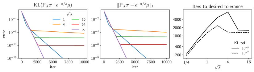
We emphasize that his behavior concerns both the global unbalanced problem (corresponding to ) as well as the domain decomposition cell problems. It was already observed in [6, Figure 5] for a fixed value of . Therefore, understanding the cause of this behavior remains an interesting topic for future investigations. In the meantime, as a practical remedy we recommend to numerically explore the position of the plateau in a given set of problems and then choose in a compromise of acceptable precision and fast convergence.
Balancing
In balanced domain decomposition [5], the Sinkhorn algorithm for the cell problems is terminated after a -half iteration, which guarantees that and thus the global -marginal is preserved during the execution of the algorithm. But some marginal error occurs on the -marginal, which means that in general and these errors will accumulate over time. In [5] a balancing step is introduced to correct this marginal error by transferring a small amount of mass between basic cells within a composite cell, in such a way that is preserved but also for each at the end of every domain decomposition iteration.
In unbalanced transport, since the marginal constraint is replaced by a more flexible marginal penalty, one might hope that such balancing procedure were unnecessary. However, as the problem will behave increasingly similar to the balanced limit, which means that it becomes increasingly sensitive to small mass fluctuations in the basic cells. Indeed we found that in practice an adapted balancing step also improves convergence of unbalanced domain decomposition.
We chose the following adaptation. For cell , let be the final Sinkhorn iterates and let be the basic cell marginals. Then perform an additional Sinkhorn half-iteration to get the marginal of the subsequent plan, that we denote by . Next, for each introduce
| (32) |
The balancing step now shifts mass horizontally (i.e., without changing its -coordinate) between the basic cells in such that for all . This is possible since . For balanced transport this reduces to the scheme of [5], since in this case and therefore . The intuition for unbalanced transport is that , obtained after an -half iteration, is a better estimate of the (unknown) optimal -marginal than , which was obtained after a -half iteration. Hence, adjusting the basic cell masses to agree with yields faster convergence. This intuition is confirmed by numerical experiments, especially for large .
4.2 Different parallelization weight functions
In this section we compare different ways and weight functions to parallelize the partition for loop in Algorithm 4. The methods and their shorthands are as follows:
sequential: The sequential Algorithm 3.
safe: The parallel algorithm with GetWeights. This is straightforward to implement but the stepsize becomes impractically small as the partition size increases.
fast: The parallel algorithm with the naive greedy choice that GetWeights always returns . This is not guaranteed to converge according to our theory and it will also frequently not converge in practice.
swift: The parallel algorithm with GetWeights, which allows a greedy update whenever it is beneficial, and falls back to GetWeights otherwise.
opt: The parallel algorithm with GetWeights. This is guaranteed to yield the largest possible instantaneous decrement, but it can become computationally expensive to solve the weight optimization problem.
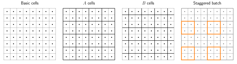
staggered: Subdivide each partition into batches of staggered cells, in such a way that neither partition contains adjacent composite cells (see Figure 5). Then apply the swift strategy to each of the subpartitions. Intuitively, for small values of the regularization and close to convergence, very little overlap between the -marginals in each of the subpartitions is expected, and thus the cell problems become approximately independent, i.e. the probability for triggering the GetWeights fallback is small and the greedy update will be applied more often.
According to Propositions 3.12, 3.14, and 3.16 all strategies (except for fast) are guaranteed to converge.
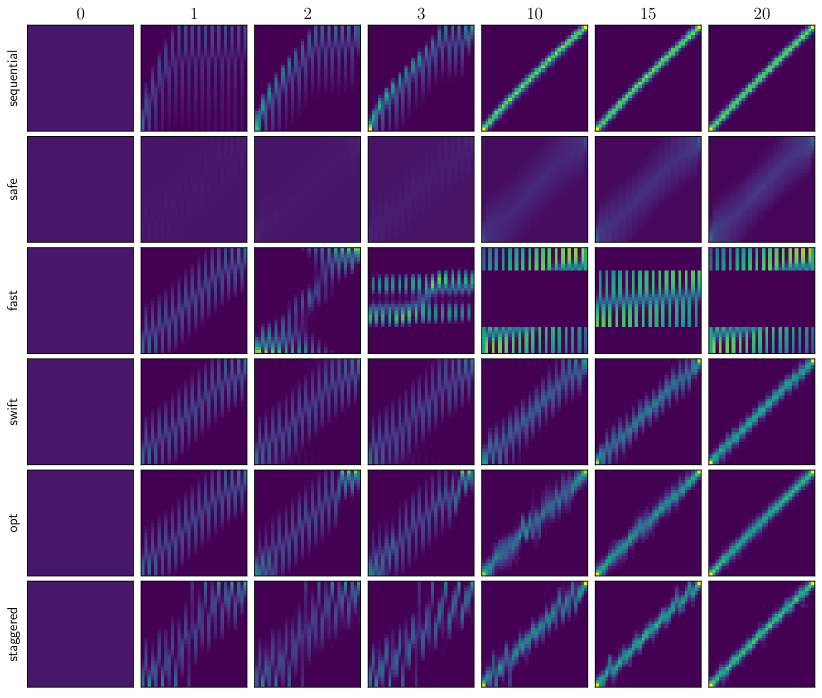
In Figures 2 and 3 we compare the different proposed strategies on a toy problem with being a homogenous discrete measure on the equispaced grid , for . The composite partition is obtained by aggregating neighboring pairs of points into composite cells, is the staggered partition with two singletons and at the beginning and the end. We set , and (i.e. the blur scale is on the order of the grid resolution). The optimal plan will be approximately concentrated along the diagonal with a blur width of a few pixels. As initial iterate we choose the product measure .
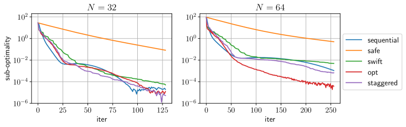
Figure 2 shows both the short and long term behavior of the domain decomposition iterations, while 3 compares the sub-optimality of the objective over time, where a reference solution was computed with a global Sinkhorn algorithm with very small tolerance. In the following we briefly discuss the behavior of each strategy.
sequential
In Figure 2 we observe a rapid formation of the diagonal structure, much faster than what we would expect in the balanced case (where we need approximately iterations, see [4]). Also unlike in the balanced case, the evolution is not symmetrical, which comes from the order in which the cell problems are solved and their interdependence. In terms of iterations, the global score is decreased in a way that is comparable with the best parallel approaches (see Figure 3), which makes sense since each cell problem can already react to the changes by the previous cells. Of course, due to the sequential nature, a single iteration will require much more time. We attribute the slight increment of the score around iteration to the inexact solution of the Sinkhorn subproblem.
safe
The small step size imposed by the safe approach leads to a very slow evolution of the iterates (see both figures) On larger problems this will become even worse, since the step size scales like . This renders the safe approach impractical for an efficient, large-scale solver.
fast
The greedy fast scheme leads to non-convergent behavior due to a lack of coordination between the cells. In the first domain decomposition iteration the cells create a surplus of mass in the central region of . The next iteration compensates for this imbalance, but since each subproblem acts on its own, they overshoot and create a new accumulation of mass at the extremes of . This oscillation pattern somewhat stabilizes into a cycle. Hence, without an additional safeguard, the fast approach fails to provide a convergent algorithm.
swift
The swift approach is a simple way to add a safeguard to the fast approach. By switching between the fast and safe strategies based on their decrements, the algorithm becomes convergent. However, the fallback to safe is rather inefficient, as can be inferred from Figure 3. Especially during the early iterations, a sharp decrement of the score (corresponding to a fast iteration) is followed by several iterations with slow decrement (corresponding to safe iterations).
opt
As shown in Figures 2 and 3, the opt strategy is among the fastest in terms of iteration numbers. Its main drawback is that computing its convex combination weights hinges on the solution of the auxiliary optimization problem
| (33) |
Although (33) is a convex optimization problem, solving it in every iteration adds considerable overhead due to the need to instantiate the global plan for different choices of .
staggered
As exemplified by Figures 2 and 3, the staggered strategy achieves fast, consistent decrements without relying on auxiliary optimization problems nor excessive calls to the safe strategy. This is achieved by the division of each partition into staggered batches, which in practice greatly reduce the overlap between cell -marginals (after some initial iterations). Although the opt strategy may provide faster decrements in terms of iteration numbers, due to its simplicity we consider the staggered strategy to be preferable, in particular on larger problems.
4.3 Large scale examples
4.3.1 Setup
Compared algorithms, implementations, and hardware
In this Section we compare unbalanced domain decomposition to the global unbalanced Sinkhorn algorithm. Our implementation for unbalanced domain decomposition is based on the GPU implementation of balanced domain decomposition described in [13, Appendix A]111Code available at https://github.com/OTGroupGoe/DomainDecomposition.. Its main features are sparse storage of cell marginals in a geometric ‘bounding box structure’, and a Sinkhorn cell solver that is tailored specifically for handling a large number of small problems in parallel. For the global Sinkhorn solver we also use the implementation discussed in [13], which compares favorably to keops/geomloss [9] in the range of problem sizes considered (see [13, Figure 10]). In the following we will refer to these two algorithms as DomDec and Sinkhorn, respectively.
The experiments were run on an Intel Xeon Gold 6252 CPU with 24 cores (we use 1) and an NVIDIA V100 GPU with 32 GB of memory.
Stopping criterion and measure truncation
We use (31) divided by (see discussion above) to measure the suboptimality error of the Sinkhorn iterations. As error threshold we use , where for DomDec is the collection of the -marginals of the cell problems the cell Sinkhorn solver is handling simultaneously, and for Sinkhorn is simply . We use , which yields a good balance between accuracy and speed.
In DomDec, the basic cell marginals are truncated at and stored in bounding box structures (see [13, Appendix] for more details).
Test data
We use the same problem data as in [5] and [13, Appendix]: images with dimensions , with and ranging from to , i.e. images between the sizes to . The images are Gaussian mixtures supported on with random variances, means, and magnitudes. For each problem size we generated 10 test images, i.e. 45 pairwise transport problems, and average the results. An example of the problem data is shown in Figure 4.
Multi-scale and -scaling
All algorithms implement the same strategy for multi-scale and -scaling as in [5, Section 6.4]. At every multiscale layer, the initial regularization strength is , where stands for the pixel size, and the final value is . In this way, the final regularization strength on a given multiscale layer coincides with the initial one in the next layer. On the finest layer is decreased further to the value implying a relatively small residual entropic blur.
Double precision
All algorithms use double floating-point precision, since single precision causes a degradation in the accuracy for problems with and small . For more details see [13, Appendix], where this behavior was originally reported.
Basic and composite partitions
We generate basic and composite partitions as in [5]: for the basic partition we divide each image into blocks of pixels (where is a divisor of the image size), while composite cells are obtained by grouping cells of the same size, as shown in Figure 5. For the cells we pad the image boundary with a region of zero density, such that all composite cells have the same size, to simplify batching. As in [5] and [13], we observe experimentally that the choice of cell size yields the best results.
staggered strategy and batching
Based on Section 4.2 we use the staggered strategy for parallelizing the unbalanced cell problems. Parallelizing the cell problems in batches of four staggered grids (see Figure 5) reduces the overlap between their -marginal supports and thus increases the chances of accepting the greedy iteration. In practice we are somewhat lenient when accepting the greedy solution, since the finite error in the cell Sinkhorn stopping criterion can sometimes lead to small increases in the objective. We allow for an increase of up to 0.5% in the primal score without triggering the safeguard. For large values of it might be practical to further increase this threshold since small deviations in the marginal lead to strong increases in the score (see also the discussion on the balancing step in Section 4.1).
Sinkhorn warm start
A drawback of the staggered strategy is that one is forced to use at least batches, which causes considerable overhead on small problems. For this reason, even in DomDec we solve the first multiscale layers with the global Sinkhorn solver, and only switch to domain decomposition starting at layer (for ), or (for ) (i.e., for small problems only the last layer is solved with domain decomposition). This combines the efficiency of GPU Sinkhorn solvers in small-to-medium sized problems with the better time complexity of domain decomposition for larger problems. The tolerance of the lower resolution Sinkhorn solver is set to one forth of the domain decomposition tolerance, with the objective of minimizing the mismatch between and the optimal first marginal, since as explained in [5] and Section 4.1 domain decomposition suffers from balancing problems when the first marginal is not kept close to optimal.
4.3.2 Results
Influence of
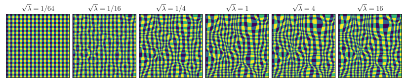
Figure 6 illustrates the influence of on the optimal transport map for an example problem. For very small mass is barely transported since the marginal discrepancy in the -terms is very cheap. As increases, more transport occurs and we asymptotically approach the balanced problem.
Runtime
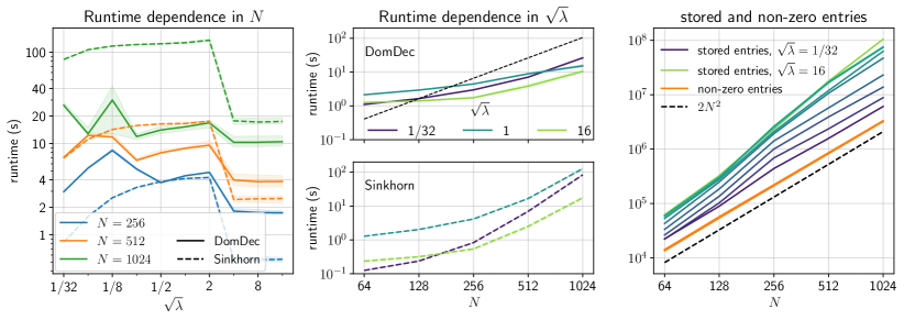
Figure 7 shows the runtime of the numerical experiments, while Table 2 reports subroutine runtime and solution quality for . We summarize the performance over all test problems by the median, since it is more robust to a few outliers where we observed convergence issues (see paragraph further below).
In Figure 7, left we can observe a steady increase in runtime for the Sinkhorn solver, followed by a sharp decline when certain value of is crossed. This is consistent with the behavior shown in Figure 1; the slightly different dependence in is due to the fact that we are now using a multiscale solver with -scaling, instead of the fixed scale and used in Figure 1. The runtime for DomDec is more consistent, with small values of appearing to be the most challenging regime. This can be explained by the fact that for small we expect more non-local changes in mass, for which domain decomposition is not as well-suited as a global Sinkhorn solver. Intermediate values of show the largest benefit of using DomDec instead of Sinkhorn.
For very large we are essentially solving a balanced problem (as exemplified by Figure 6). In this regime DomDec outperforms Sinkhorn on large problems, although it does not match the speed-up reported for balanced transport in [13]. This is mainly due to two reasons: First, the unbalanced algorithm requires several steps that cause additional overhead, such as the Newton iteration in the Sinkhorn subsolver (see (27) and discussion below), and the calculation of the global -marginal and (we will comment on this further below). Besides, the balanced problem allows for a series of performance tricks (e.g. batches of arbitrary size, clustering of the composite cells’ sizes to maximize the efficiency of the Sinkhorn iteration) that are hard to adapt to unbalanced DomDec when employing the staggered parallelization strategy.
Figure 7 shows the runtime in terms of for fixed . The scaling in of DomDec and Sinkhorn agrees well with that reported in [13] for the balanced case, with DomDec featuring a larger constant overhead for the reasons commented above, but a slower increase with . Hence for large DomDec is faster than Sinkhorn.
In Table 2 we report more detailed statistics about the runtime and solution quality for . We observe that the Sinkhorn warm start —used to solve the first multiscale layers— claims a sizable share of the total runtime. Of the remaining time (when domain decomposition is running) about 60% corresponds to the subproblem solving, 10% to the computation of , about 8% for manipulation of the sparse structure containing the cell -marginals , and another 8% to the balancing procedure. Refinement, batching and other minor operations only account for a negligible fraction. Within the solution of the cell subproblems, the Newton subroutine required to compute the -iteration (cf. (27) and discussion below) claims 47% of the subproblem solving time, even after implementing it directly in CUDA. It would be interesting to investigate if this routine can be improved further.
Issues with non-convergence
In about 1% of cell problems the subsolver in DomDec failed to reach the prescribed error goal and terminated before convergence. This happened in cases where was large and it is connected to the issue described in Figure 1. It was possible to restore convergence by further decreasing the tolerance of the warm start Sinkhorn, which indicates that the problem is connected to mass discrepancies in the initial plan.
The safe safeguard was only triggered in the 1% of failing instances mentioned above. In the other cases the greedy stage of the staggered strategy worked without issues. If the threshold for the safe method is lowered (which increases the frequency of its calls) more problems outside this 1% cohort invoke the safe method at some stage. This does not hinder the Sinkhorn subsolver, but causes that more domain decomposition iterations are needed for convergence, since the safe method imposes a rather small step size. Therefore, we recommend to use the algorithm with the settings described above and to only increase the precision goal for the Sinkhorn warm start when a problem with convergence occurs.
| image size | 6464 | 128128 | 256256 | 512512 | 10241024 |
|---|---|---|---|---|---|
| total runtime (seconds) | |||||
| DomDec | 2.14 | 2.94 | 4.44 | 8.88 | 15.3 |
| Sinkhorn | 1.28 | 2.03 | 4.14 | 16.6 | 127 |
| time spent in DomDec’s subroutines (seconds) | |||||
| warm up Sinkhorn | 0.915 | 1.78 | 3.06 | 6.14 | 6.21 |
| Sinkhorn subsolver | 0.675 | 0.552 | 0.642 | 1.45 | 5.45 |
| bounding box processing | 0.225 | 0.235 | 0.250 | 0.307 | 0.770 |
| compute | 0.120 | 0.121 | 0.128 | 0.183 | 0.883 |
| DomDec solution quality | |||||
| marginal error | 2.1e-04 | 8.6e-05 | 1.9e-05 | 4.2e-06 | 4.7e-06 |
| marginal error | 5.5e-03 | 3.9e-03 | 3.4e-03 | 3.2e-03 | 3.2e-03 |
| relative primal-dual gap | 1.0e-03 | 2.1e-03 | 3.7e-03 | 2.4e-03 | 3.5e-03 |
| Sinkhorn solution quality | |||||
| marginal error | 6.3e-03 | 6.3e-03 | 6.3e-03 | 6.3e-03 | 6.3e-03 |
| relative primal-dual gap | 1.1e-03 | 2.4e-03 | 4.5e-03 | 2.7e-03 | 3.7e-03 |
Solution quality
Since the unbalanced optimality conditions (25) tend to the balanced optimality conditions as , we call the difference between and the -marginal error, and define the -marginal error analogously. Table 2 gives the -marginal error for DomDec and Sinkhorn and the -marginal error for DomDec (since Sinkhorn ends in a -iteration, its -marginal error is zero). We observe a similar -marginal error for DomDec and Sinkhorn, with DomDec being slightly better. The -marginal error for DomDec is typically several orders of magnitude smaller than the -marginal error.
Sparsity
As shown in Figure 7, right, the number of non-zero entries grows approximately linearly with the image resolution , with an essentially identical behavior for all values of . This is similar to the balanced case as reported in [5, 13].
On the other hand, the required memory increases with up to the level reported in [13] for balanced domain decomposition on GPUs. This can be understood with the help of Figure 6: for small there is little actual transport happening and the support of the basic cell -marginals is close to that of the -marginals . As a result, the bounding box structure stores the cell -marginals quite efficiently, since their support is close to being square-shaped. As increases, the shapes of the cell -marginals become more complex and diverse as in the balanced problem, and the bounding box storage becomes less efficient.
This trend is currently the limiting factor for further increasing the problem size in DomDec. We expect that this could be improved by more sophisticated storage methods for the cell -marginals, such as alternating between a box-based representation for the subproblem solving (enhancing the efficiency of the Sinkhorn iterations) and a more classical sparse representation for storage between iterations.
Conclusion
Previous work has demonstrated the efficiency of domain decomposition for balanced optimal transport. Generalizing domain decomposition to unbalanced transport involved addressing both theoretical and numerical challenges. Our numerical experiments show that unbalanced domain decomposition compares favorably to a global Sinkhorn solver for a wide range of values of in medium to large problems. An important task for future work is an improved memory efficiency for the bounding box data structure and a faster inner Newton step in the Sinkhorn iteration.
References
- [1] Florian Beier, Johannes von Lindheim, Sebastian Neumayer, and Gabriele Steidl. Unbalanced multi-marginal optimal transport. Journal of Mathematical Imaging and Vision, 65(3):394–413, Jun 2023.
- [2] Jean-David Benamou. A domain decomposition method for the polar factorization of vector-valued mappings. SIAM J. Numer. Anal., 32(6):1808–1838, 1994.
- [3] Mauro Bonafini, Ismael Medina, and Bernhard Schmitzer. Asymptotic analysis of domain decomposition for optimal transport (arxiv v1 version), 2021.
- [4] Mauro Bonafini, Ismael Medina, and Bernhard Schmitzer. Asymptotic analysis of domain decomposition for optimal transport. Numerische Mathematik, 153:451–492, 2023.
- [5] Mauro Bonafini and Bernhard Schmitzer. Domain decomposition for entropy regularized optimal transport. Numerische Mathematik, 149:819–870, 2021.
- [6] Lenaic Chizat, Gabriel Peyré, Bernhard Schmitzer, and François-Xavier Vialard. Scaling algorithms for unbalanced transport problems. Mathematics of Computation, 87, 07 2016.
- [7] Lénaïc Chizat, Gabriel Peyré, Bernhard Schmitzer, and François-Xavier Vialard. Unbalanced optimal transport: Dynamic and Kantorovich formulations. Journal of Functional Analysis, 274(11):3090–3123, 2018.
- [8] M. Cuturi. Sinkhorn distances: Lightspeed computation of optimal transportation distances. In Advances in Neural Information Processing Systems 26 (NIPS 2013), pages 2292–2300, 2013.
- [9] Jean Feydy. Geometric data analysis, beyond convolutions. PhD thesis, Université Paris-Saclay, 2020.
- [10] Charlie Frogner, Chiyuan Zhang, Hossein Mobahi, Mauricio Araya-Polo, and Tomaso Poggio. Learning with a Wasserstein loss. Advances in Neural Information Processing Systems 28 (NIPS 2015), 2015.
- [11] Jean-Baptiste Hiriart-Urruty and Claude Lemaréchal. Convex Analysis and Minimization Algorithms II. Springer-Verlag Berlin Heidelberg, 1993.
- [12] Matthias Liero, Alexander Mielke, and Giuseppe Savaré. Optimal entropy-transport problems and a new Hellinger–Kantorovich distance between positive measures. Inventiones mathematicae, 211(3):969–1117, 2018.
- [13] Ismael Medina and Bernhard Schmitzer. Flow updates for domain decomposition of entropic optimal transport. arXiv:2405.09400, 2024.
- [14] Gabriel Peyré and Marco Cuturi. Computational optimal transport. Foundations and Trends in Machine Learning, 11(5–6):355–607, 2019.
- [15] Filippo Santambrogio. Optimal Transport for Applied Mathematicians, volume 87 of Progress in Nonlinear Differential Equations and Their Applications. Birkhäuser Boston, 2015.
- [16] C. Villani. Optimal Transport: Old and New, volume 338 of Grundlehren der mathematischen Wissenschaften. Springer, 2009.