FlowMRI-Net: A generalizable self-supervised physics-driven 4D Flow MRI reconstruction network for aortic and cerebrovascular applications

Abstract

In this work, we propose FlowMRI-Net, a novel deep learning-based framework for fast reconstruction of accelerated 4D flow magnetic resonance imaging (MRI) using physics-driven unrolled optimization and a complex-valued convolutional recurrent neural network trained in a self-supervised manner. The generalizability of the framework is evaluated using aortic and cerebrovascular 4D flow MRI acquisitions acquired on systems from two different vendors for various undersampling factors (R=8,16,24) and compared to state-of-the-art compressed sensing (CS-LLR) and deep learning-based (FlowVN) reconstructions. Evaluation includes quantitative analysis of image magnitudes, velocity magnitudes, and peak velocity curves. FlowMRI-Net outperforms CS-LLR and FlowVN for aortic 4D flow MRI reconstruction, resulting in vectorial normalized root mean square errors of $0.239\pm 0.055$, $0.308\pm 0.066$, and $0.302\pm 0.085$ and mean directional errors of $0.023\pm 0.015$, $0.036\pm 0.018$, and $0.039\pm 0.025$ for velocities in the thoracic aorta for R=16, respectively. Furthermore, FlowMRI-Net outperforms CS-LLR for cerebrovascular 4D flow MRI reconstruction, where no FlowVN can be trained due to the lack of a high-quality reference, resulting in a consistent increase in SNR of around $6~{}dB$ and more accurate peak velocity curves for R=8,16,24. Reconstruction times ranged from 1 to 7 minutes on commodity CPU/GPU hardware. FlowMRI-Net enables fast and accurate quantification of aortic and cerebrovascular flow dynamics, with possible applications to other vascular territories. This will improve clinical adaptation of 4D flow MRI and hence may aid in the diagnosis and therapeutic management of cardiovascular diseases. The implementation code, data, and pre-trained weights will be made available at gitlab.ethz.ch/ibt-cmr/publications/flowmri_net.

4D flow MRI, aortic and cerebrovascular flow, deep learning, reconstruction

1 Introduction

Cardiovascular diseases remain a leading cause of morbidity and mortality worldwide, necessitating effective diagnostic tools for early detection and management. Flow magnetic resonance imaging (MRI) is a non-invasive and non-ionizing imaging technique capable of quantifying 4D (3D+time) blood flow dynamics [1], from which various hemodynamic parameters can be inferred such as wall shear stress [2], pressure gradients [3], and pulse wave velocity [4], with applications including the cardiovascular system (aorta, pulmonary arteries, abdomen, and liver), heart (atria, ventricles, and coronary arteries), and head/neck (carotid arteries and cerebral arteries and veins) [5]. However, clinical adaptation of 4D flow MRI [6, 7] has been hampered by its long scan time, particularly for smaller vasculatures that require higher spatial resolutions for accurate flow quantification. Historically, scan times of MRI acquisitions have been successfully reduced by undersampling the acquired data and resolving the resulting aliasing artifacts using traditional reconstruction algorithms such as parallel imaging (PI) [8, 9, 10] and compressed sensing (CS) [11] methods, which exploit redundancies among multi-channel coils and compressibility of images, respectively. Although these methods could be used for frame-by-frame reconstruction of dynamic MRI, methods that also exploit temporal redundancies such as k-t BLAST (Broad-use Linear Acquisition Speed-up Technique) [12] and it temporally constrained extension k-t PCA (Principal Component Analysis) [13] have been shown to improve reconstruction performance, including for 4D flow MRI [14, 15]. More recently, deep learning (DL)-based reconstructions have been demonstrated to enable even higher undersampling rates and/or faster reconstruction times, by exploiting redundancies that are implicitly learned from the acquired data [14]. Although a conceptually straightforward end-to-end mapping between undersampled k-space and fully-sampled image could be learned, this requires large amounts of paired data for training and does not take the known imaging physics into account [15]. Currently, the state-of-the-art is defined by unrolled optimization algorithms using physics-driven DL, pioneered by the variational network (VN) approach [16], which combine the expressiveness of DL with the robustness of traditional optimization algorithms [17]. Similar success has been achieved for 4D flow MRI by FlowVN, which trains an improved VN in a supervised manner using PI-reconstructed images as reference [18]. For aortic stenosis patients, it was shown that the relative error of peak velocity magnitudes for 10-fold retrospectively undersampled data was lower for FlowVN (19.7%) than CS (22.1%), with reconstruction times of 21 s and 10 min, respectively. For 13-fold prospectively undersampled data, FlowVN and CS resulted in peak velocity/flow deviations from reference of -1.59/-0.05% and -1.18/0.36%, respectively. However, FlowVN’s high graphical processing unit (GPU) memory demands and its reliance on reference data may limit its applications to relatively small k-space matrices, such as the demonstrated aortic Cartesian 4D flow MRI use case. Self-supervised learning strategies can aid to generalize to applications where high-quality reference data are impractical or even infeasible to acquire, for example due to higher spatial and/or temporal resolution or multiple velocity encodings [19, 20, 21]. The recently proposed training strategy called self-supervised learning via data undersampling (SSDU) [22] splits the undersampled data into two disjoint sets, one for network input and one for defining the training loss. SSDU has been successfully applied for reconstructions of various cardiac MRI applications [23, 24, 25, 26]. In the present work we propose FlowMRI-Net, facilitating reconstruction from highly undersampled data within clinically feasible time budgets and with improved velocity quantification relative to state-of-the-art CS and FlowVN by efficiently exploiting redundancies in spatiotemporal and velocity-encoding dimensions using a complex-valued multi-coil unrolled network. It is demonstrated that FlowMRI-Net’s memory-efficient self-supervised learning strategy allows for generalizability to different 4D flow MRI applications. We demonstrate this generalizability for aortic and cerebrovascular 4D flow MRI, where no high-quality fully sampled data is available.

2 Methods

The standard way to encode a time-resolved three-dimensional velocity-vector field is using a four-point referenced encoding scheme, with three scans encoding the velocity of each Cartesian direction independently in the phase of the signal using a bipolar gradient and one non-velocity-encoding scan measuring the background phase (number of velocity-encodings $N_{V}=4$) [27]. The velocity field can then be extracted from the phase difference of these resulting complex-valued MR images $\boldsymbol{x}\in\mathbb{C}^{P}(P=N_{V}\times N_{T}\times N_{X}\times N_{Y}\times N_{Z})$), with number of cardiac bins $N_{T}$ and number of sampling points in $x,y,$ and $z$ direction $N_{X}$, $N_{Y}$, and $N_{Z}$, respectively. Because of the high dimensionality of $\boldsymbol{x}$, undersampling in k-space is required to make the acquisition time clinically feasible. Let $\boldsymbol{y_{i}}\in\mathbb{C}^{Q}(i\in\{1,...,N_{C}\},Q\ll P)$ represent the undersampled k-space measured by the $i$-th out of $N_{C}$ receiver coils. The forward MRI acquisition process can then be modelled as

$$\boldsymbol{y}_{i}=\boldsymbol{E_{i}}\boldsymbol{x}=\boldsymbol{D}\mathcal{\boldsymbol{F}}\boldsymbol{S}_{i}\boldsymbol{x},$$ (1)

with forward encoding operator $\boldsymbol{E_{i}}$, consisting of the $i$-th coil sensitivity maps $\boldsymbol{S}_{i}\in\mathbb{C}^{N_{X}\times N_{Y}\times N_{Z}}$, spatial Fourier transform $\mathcal{\boldsymbol{F}}$, and undersampling mask given by the diagonal matrix $\boldsymbol{D}$. To reconstruct $\boldsymbol{x}$ from $\boldsymbol{y}$, the resulting ill-posed inverse problem can be solved using the following unconstrained optimization:

$$\underset{\boldsymbol{x}}{\operatorname{argmin}}\frac{\lambda}{2}\sum_{i=1}^{N_{c}}\left\|\boldsymbol{D}\mathcal{\boldsymbol{F}}\boldsymbol{S_{i}}\boldsymbol{x}-\boldsymbol{y}_{\boldsymbol{i}}\right\|_{2}^{2}+\mathcal{R}(\boldsymbol{x}),$$ (2)

with weight $\lambda$ balancing the data consistency (DC) and regularization $\mathcal{R}$.

2.1 MR image reconstruction using unrolled network

To solve (2) we use the variable splitting algorithm with quadratic penalties as proposed for VS-Net (variable splitting network) [28] by introducing two auxiliary variables $\boldsymbol{w_{i}}$ and $\boldsymbol{z}$ with quadratic penalty weights $\alpha$ and $\beta$, respectively:

$$\underset{\boldsymbol{x},\boldsymbol{z},\boldsymbol{w_{i}}}{\operatorname{argmin}}\frac{\lambda}{2}\sum_{i=1}^{N_{c}}\left\|\boldsymbol{D}\mathcal{\boldsymbol{F}}\boldsymbol{w_{i}}-\boldsymbol{y_{i}}\right\|_{2}^{2}+\mathcal{R}(\boldsymbol{z})+\frac{\alpha}{2}\sum_{i=1}^{N_{c}}\left\|\boldsymbol{w_{i}}-\boldsymbol{S_{i}x}\right\|_{2}^{2}+\frac{\beta}{2}\left\|\boldsymbol{x}-\boldsymbol{z}\right\|_{2}^{2}.$$ (3)

This formulation decouples the regularization from the DC term and prevents any dense matrix inversions later on. To solve this multivariable optimization problem, alternate minimization over $\boldsymbol{x}$, $\boldsymbol{w_{i}}$, and $\boldsymbol{z}$ is performed:

$$\boldsymbol{z^{n}} =\underset{\boldsymbol{z}}{\operatorname{argmin}}\frac{\beta}{2}\left\|\boldsymbol{x^{n-1}}-\boldsymbol{z}\right\|_{2}^{2}+\mathcal{R}(\boldsymbol{z}),$$ (4a)

$$\boldsymbol{w^{n}_{i}} =\underset{\boldsymbol{w_{i}}}{\operatorname{argmin}}\frac{\lambda}{2}\sum_{i=1}^{N_{c}}\left\|\boldsymbol{D}\mathcal{\boldsymbol{F}}\boldsymbol{w_{i}}-\boldsymbol{y_{i}}\right\|_{2}^{2}+\frac{\alpha}{2}\sum_{i=1}^{N_{c}}\left\|\boldsymbol{w_{i}}-\boldsymbol{S_{i}x^{n-1}}\right\|_{2}^{2},$$ (4b)

$$\boldsymbol{x^{n}} =\underset{\boldsymbol{x}}{\operatorname{argmin}}\frac{\alpha}{2}\sum_{i=1}^{N_{c}}\left\|\boldsymbol{w_{i}^{n}}-\boldsymbol{S_{i}x}\right\|_{2}^{2}+\frac{\beta}{2}\left\|\boldsymbol{x}-\boldsymbol{z^{n}}\right\|_{2}^{2},$$ (4c)

with $n\in\{1,...,N\}$ denoting the $m$-th iteration and $\boldsymbol{x^{0}}$ being initialized as a zero-filled reconstruction, where (4a) is the proximal operator of the prior $\mathcal{R}$ and (4b) and (4c) have closed-form solutions:

$$\boldsymbol{z^{n}} =\operatorname{prox}_{\mathcal{R}}(\boldsymbol{x^{n-1}}),$$ (5a)

$$\boldsymbol{w^{n}_{i}} =\boldsymbol{\mathcal{F}^{-1}}\left(\left(\lambda\boldsymbol{D^{T}D}+\alpha\boldsymbol{I}\right)^{-1}\left(\lambda\boldsymbol{D^{T}y_{i}}+\alpha\boldsymbol{\mathcal{F}S_{i}x^{n-1}}\right)\right),$$ (5b)

$$\boldsymbol{x^{n}} =\left(\alpha\sum_{i=1}^{N_{c}}\boldsymbol{S_{i}^{H}}\boldsymbol{S_{i}}+\beta\boldsymbol{I}\right)^{-1}\left(\alpha\sum_{i=1}^{N_{c}}\boldsymbol{S_{i}^{H}}\boldsymbol{w_{i}^{k}}+\beta\boldsymbol{z^{n}}\right).$$ (5c)

Here, (5a) can be defined as a learnable denoising operation using a neural network (denoising block). Note that the inversions in (5b) and (5c) are performed on diagonal matrices, making them element-wise operations. When defining noise level $\nu^{n}=\frac{\lambda}{\lambda+\alpha}$ per iteration $n$, (5b) turns into a coil-wise weighting averaging that sums the measured k-space $\nu^{n}\boldsymbol{y_{i}}$ and reconstructed k-space $(1-\nu^{n})\boldsymbol{\mathcal{F}S_{i}x^{n-1}}$ for sampled ($\boldsymbol{D_{jj}}=1$) points and copies the reconstructed k-space $\boldsymbol{\mathcal{F}S_{i}x^{n-1}}$ for unsampled ($\boldsymbol{D_{jj}}=0$) points (DC block). Similarly, when defining weighting $\mu^{n}=\frac{\alpha}{\alpha+\beta}$ per iteration $n$ and assuming normalized $\boldsymbol{S_{i}}$, (5c) turns into a weighted averaging that sums the output of the denoising block $\mu^{n}\sum_{i=1}^{N_{C}}\boldsymbol{S_{i}^{H}}\boldsymbol{w_{i}^{n}}$ and DC block $(1-\mu^{n})\boldsymbol{z}^{n}$ (weighted-averaging (WA) block). The denoising, DC, and WA blocks are repeated for a fixed number of $N$ units in the unrolled network, where both $\nu^{n}$ and $\mu^{n}$ are learnable parameters per unit $n$ and are passed through a Sigmoid function $\sigma$ to guarantee proper averaging.

2.2 Data acquisition

Aortic data were acquired in 15 volunteers (age=28.1$\pm$3.9 years, m/f=2/3 after written informed consent and according to institutional and ethical guidelines on a Philips Ambition 1.5T system (Philips Healthcare, Best, the Netherlands) with a 28-channel cardiac coil using a retrospectively electrocardiogram (ECG)-triggered four-point referenced phase-contrast gradient-echo sequence during free breathing. The sagittal oblique field-of-view (FOV) = 360 mm $\times$ 228-298 mm $\times$ 60 mm (minimized in phase-encoding direction to maximize scan efficiency whilst preventing fold-over) covered the thoracic aorta, using an acquired spatial resolution of 2.5 mm $\times$ 2.5 mm $\times$ 2.5 mm, an acquired temporal resolution of 48.9 ms, velocity encoding (venc) = 150 cm/s, echo time (TE) = 3.1 ms, repetition time (TR) = 5.4 ms, and flip angle (FA) = 15^∘. Cartesian elliptical pseudo-spiral Golden angle data were acquired for approximately one hour per volunteer, from which four equally populated respiratory bins were extracted using the Philips VitalEye camera [29], where only the end-expiratory bin was considered in this work, resulting in an effective undersampling factor between 3 and 4, depending on the heartrate and FOV. A CS-based reconstruction (please refer to Experiment and evaluation for more details) of these relatively densely sampled data were used for evaluation. Due to the Golden angle sampling, paired prospectively-undersampled scans could be extracted from the acquisition by omitting the last number of readouts, depending on the desired undersampling factor. As an additional reference, a fully sampled two-point 2D referenced phase-contrast gradient-echo was acquired for each of the Cartesian directions during breath-holding. The axial slice with a FOV = 350 mm $\times$ 200-425 mm (maximized in phase-encoding direction to maximize the signal-to-noise ratio (SNR) for the longest possible breath-hold per subject) cut the ascending and descending aorta at the level of the right pulmonary trunk, using an acquired spatial resolution of 2.5 mm $\times$ 2.5 mm $\times$ 8 mm, an a temporal resolution of 45.8 ms, venc = 150 cm/s, TE = 2.6 ms, TR = 4.5 ms, and FA = 15^∘.

Cerebrovascular data were acquired in 10 volunteers (age = 25.2 $\pm$ 3.1 years, m/f = 3/2) after written informed consent and according to institutional and ethical guidelines on a Siemens Vida 3T system (Siemens Healthineers, Erlangen, Germany) with a 64-channel head-neck coil using a retrospectively peripheral pulse unit (PPU)-triggered four-point referenced phase-contrast gradient-echo sequence. The axially oblique FOV = 240 mm $\times$ 183 mm $\times$ 64 mm covered the circle of Willis (CoW) and the confluence of sinuses, using an acquired spatial resolution of 0.8 mm $\times$ 0.8 mm $\times$ 0.8 mm, an acquired temporal resolution of 55.8 ms, venc = 100 cm/s, TE = 4.14 ms, TR = 6.98 ms, and FA = 13^∘. Each volunteer was scanned using a Cartesian 8-fold pseudo-random sampling pattern and one volunteer was also scanned using a 2-fold generalized autocalibrating partial parallel acquisition (GRAPPA) [9] with 54 reference lines and a reduced FOV = 240 mm $\times$ 171 mm $\times$ 48 mm used as a reference to test reconstruction fidelity.

2.3 Data pre-processing

The raw aortic and cerebrovascular data were parsed using PRecon (GyroTools LLC, Zurich, Switzerland) and twixtools [30], respectively. The complex-valued Cartesian k-space data $\boldsymbol{y}$ were acquired with a fully sampled readout dimension, allowing the k-space to be split into $N_{X}$ subvolumes. Estimation of coil sensitivities $\boldsymbol{S}$ from the time-averaged k-space data and subsequent compression into $N_{C}=10$ virtual coils were performed using the Berkeley Advanced Reconstruction Toolbox (BART) [31]. All velocity-encodings were acquired in an interleaved manner and jointly reconstructed by using them as feature channels of the network input, which allows their redundancies to be exploited [32]. Note that the real and imaginary components do not need to be separated in the feature channel dimension because FlowMRI-Net is complex-valued. Because only a small subset of each cerebrovascular volume contains voxels with motion/flow, an automatic sliding threshold segmentation [33] was performed on the time-averaged complex difference volumes [34] and only slices with more than 0.2% vessel content were considered for training.

2.4 Network architecture and training

The proposed unrolled network architecture and its self-supervised training scheme can be seen in Fig. 1a (see section 2.1). For the denoising block we adopted a variation of the convolutional recurrent neural network (CRNN)-MRI [35], with four bidirectional CRNN layers that evolve recurrence over both temporal and iteration dimensions and one CNN layer. We used 2D complex-valued convolutions applied over spatial $y,z$ dimensions with kernel size $k=3$, number of filters $f=25$, and $N=10$ unrolling units that share their weights and biases. The complex-valued phase-preserving modReLU, a modified rectified linear unit (ReLU) [36] proposed for complex-valued RNNs, is used as activation function [37]:

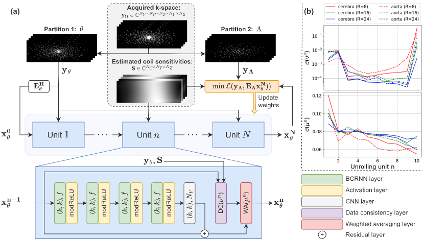
Figure 1: An overview of the self-supervised learning scheme of FlowMRI-Net. (a) The acquired k-space data $\boldsymbol{y_{\Omega}}$ are randomly partitioned into disjoint sets $\Theta$ and $\Lambda$. Partition $\Theta$ is used as input for the neural network with $N$ unrolling units, exploiting spatiotemporal redundancies in BCRNN and CNN layers (with kernel size k and number of filters $f$ or $N_{V}$) and enforcing point-wise data consistency in DC layers, which are combined in the WA layer. The resulting reconstruction $\boldsymbol{x^{N}_{\Theta}}$ is transformed to k-space and compared to the heldout second partition $\boldsymbol{y_{\Lambda}}$ using a normalized L1-L2 loss. (b) The Sigmoid $\sigma(.)$ of the learnable noise level $\nu^{n}$ (for DC layers) and learnable weight $\mu^{n}$ (for WA layers) are shown for each of the $N=10$ unrolling units trained using aortic and cerebrovascular data for different undersampling factors (R).

$$\operatorname{modReLU}(z)=\left\{\begin{aligned} (|z|+b)\frac{s}{|z|},&\text{ if }|z|+b\geq 0\\ 0,&\text{ if }|z|+b<0\end{aligned}\right.,$$ (6)

where $b$ is a real-valued bias parameter learnable for each feature map. The input of this denoising block is summed with its output by a residual connection. In parallel, the input is fed to the DC block, whose output is merged with the output of the denoising block in the WA block. The learnable noise $\nu^{n}$ (for DC layers) and learnable weights $\mu^{n}$ (for WA layers) for each unrolling unit n can be seen in Fig. 1b. Similar patterns can be seen for aortic and cerebrovascular reconstructions at different undersampling factors: an initial decrease in $\nu^{n}$ with every unrolling unit resulting in an increased weight of the acquired samples during DC, with more weight on the predicted samples for the final layers, and a gradual decrease of $\mu^{n}$ in the WA layers resulting in increasingly more weight on the DC output compared to the denoising block output.

To lower GPU memory demands at the cost of training time, gradient checkpointing was used per unrolling unit to recompute intermediate activations during backpropagation rather than saving them all during the forward pass [38]. Furthermore, tensors that were saved in the forward pass can be offloaded and stored on the central processing units (CPUs) [39].

Given the acquired k-space $\boldsymbol{y_{\Omega}}$ and estimated coil sensitivities $\boldsymbol{S}$, the sampled locations $\Omega$ are partitioned into two disjoint sets $\Theta$ and $\Lambda$. The zero-filled image of the first set, computed using the adjoint $\boldsymbol{E^{H}_{\Theta}}$ of the forward operator $\boldsymbol{E_{\Theta}}$, was used as network input and its k-space $\boldsymbol{y_{\Theta}}$ was used for DC. The k-space of the second set $\boldsymbol{y_{\Lambda}}$ was used for defining the loss. The partitioning was performed using uniform random sampling with an 80/20 split, where set $\Theta$ always contained the circular center of k-space with radius 3 for training stability. Note that during inference, no partitioning is necessary and $\boldsymbol{y_{\Omega}}$ can be used as network input. In the original multi-mask SSDU setup [40], each partition was randomly repeated for a fixed number of times per measurement, where too many partitions (considered to be data augmentations) resulted in overfitting [41]. However, such overfitting was never observed in any of our experiments, attributable to the relatively small number of learnable parameters ($\sim 10^{4}$) compared to the number of data samples per measurement ($\sim 10^{6}$). Accordingly, the partitioning was randomized for each iteration. For the training loss, reconstructed image $\boldsymbol{x^{N}_{\Theta}}$ was converted to k-space $\boldsymbol{y^{N}_{\Theta}}=\boldsymbol{E_{\Lambda}}\boldsymbol{x^{N}_{\Theta}}=\boldsymbol{D_{\Lambda}\mathcal{F}}\boldsymbol{Sx^{N}_{\Theta}}$ and compared to the left-out set $\boldsymbol{y_{\Lambda}}$ using a point-wise normalized L1-L2 loss [22]:

$$\mathcal{L}\left(\boldsymbol{y_{\Lambda}},\boldsymbol{y_{\Theta}^{N}}\right)=\frac{\left\|\boldsymbol{y_{\Lambda}}-\boldsymbol{y_{\Theta}^{N}}\right\|_{2}}{\left\|\boldsymbol{y_{\Lambda}}\right\|_{2}}+\frac{\left\|\boldsymbol{y_{\Lambda}}-\boldsymbol{y_{\Theta}^{N}}\right\|_{1}}{\left\|\boldsymbol{y_{\Lambda}}\right\|_{1}}.$$ (7)

This self-supervised loss was optimized using the Adam algorithm [42] with a batch size of 1 and a learning rate of $5\times 10^{-4}$ with a cosine annealing to 0 over 50 epochs (equivalent to $5.9\times 10^{4}$ and $6.5\times 10^{4}$ iterations for aortic and cerebrovascular data, respectively). All training was performed using Pytorch 2.3.1 [43] with Pytorch Lightning 2.2.0 [44] on an Nvidia Titan RTX GPU with 24GB memory and a 32-core Intel Xeon Gold 6130 CPU running at 2.10 GHz with 188GB memory. For the aortic data, the 15 volunteers were split into 9, 1, and 5 for training, validation, and testing, respectively. All hyperparameter were optimized using the validation set of the aortic data and were kept the same for reconstructions of the cerebrovascular data, where only 1 of the 10 volunteers had a reference acquisition (see section 2.2). Consequently, its 10 volunteers were split into 9 for training and 1 for testing.

2.5 Experiments and evaluation

The aortic data were reconstructed for two prospective undersampling factors (R=8,16) using FlowMRI-Net, FlowVN, and a GPU-accelerated CS using locally low rank (LLR) [45] regularization (CS-LLR). The hyperparameters of FlowVN and CS-LLR were optimized using the validation set. FlowVN was trained in the end-to-end fashion using the CS-LLR reconstruction of the relatively densely sampled (R=4) acquisition for the loss calculations of its supervised training. Although the original FlowVN implementation used retrospectively-undersampled data from its reference scans with additional k-space noise as network input during training, we directly input the prospectively-undersampled scans, resulting in less overfitting and a fairer comparison to CS-LLR and FlowMRI-Net. For testing, all aortic reconstructions were compared relative to CS-LLR (R=4). Quantitative metrics included the normalized peak-systolic root-mean-square error (nRMSE) of the image magnitude:

$$\operatorname{nRMSE}_{m}\left(a,a^{*}\right)=\sqrt{\frac{\sum\left|a-a^{*}\right|^{2}}{\sum\left|a^{*}\right|^{2}}},$$ (8)

for magnitude images $a$ and $a^{*}$, the vectorial nRMSE of velocities inside the region of interest (ROI) in the thoracic aorta:

$$\operatorname{nRMSE}_{v}(\boldsymbol{u},\boldsymbol{v})=\sqrt{\frac{\sum_{i\in ROI}\left\|\boldsymbol{u}_{\boldsymbol{i}}-\boldsymbol{v}_{\boldsymbol{i}}\right\|^{2}}{\sum_{i\in ROI}\left\|\boldsymbol{v}_{i}\right\|^{2}}},$$ (9)

for vector fields $\boldsymbol{u}$ and $\boldsymbol{v}$, and the mean directional error (mDirErr) [46] of velocities in the ROI:

$$\operatorname{mDirErr}(\boldsymbol{u},\boldsymbol{v})=\frac{1}{|ROI|}\sum_{i\in ROI}1-\frac{\left|\boldsymbol{u}_{\boldsymbol{i}}\cdot\boldsymbol{v}_{\boldsymbol{i}}\right|}{\left\|\boldsymbol{u}_{\boldsymbol{i}}\right\|\left\|\boldsymbol{v}_{\boldsymbol{i}}\right\|}.$$ (10)

Furthermore, the velocity curves during peak systole and peak velocity magnitude in the ascending aorta of the reconstructions were compared to the fully sampled 2D breath-hold reference (2D REF) acquisitions in feet-head (FH), right-left (RL), and anterior-posterior (AP) direction. The peak velocity magnitude was computed by determining the spatiotemporal coordinate with the highest velocity in FH direction within the eroded ROI and extracting the velocities in RL and AP direction at that same coordinate. Velocity curves were determined by tracing that coordinate over time for each encoding direction. The time-dependent 2D cross-sections of the ascending aorta were semi-automatically segmented using ITK-SNAP’s snake evolution algorithm [47] and the time-dependent 3D intra-vessel volumes of the thoracic aorta were automatically segmented using an in-house 3D nnU-net [48], starting at the sinotubular junction and excluding the brachiocephalic, left common carotid, and left subclavian arteries [49].

The 8-fold prospectively undersampled cerebrovascular data were further undersampled retrospectively using random Gaussian sampling (R=16,24) and were reconstructed using FlowMRI-Net and CS-LLR. Because high-quality reference data are unavailable, no FlowVN could be trained and reconstructions were predominantly qualitatively compared to the 2-fold undersampling GRAPPA reconstruction for the testing set, where the SNR was quantitatively compared for patches placed in homogeneous parts of the brainstem and white matter of the image magnitude ($a_{patch}$), assuming Gaussian noise:

$$\operatorname{SNR}(a_{patch})=20\operatorname{log}_{10}\frac{\operatorname{mean}(a_{patch})}{\operatorname{std}(a_{patch})},$$ (11)

where $\operatorname{std}(.)$ computes the standard deviation. The GRAPPA reconstruction was rigidly registered to the FlowMRI-Net reconstruction using SimpleITK’s 3D Euler transform [50]. The 3D segmentations for the velocity curves of the left and right middle cerebral arteries (LMCA/RMCA) at the M1 level, left and right internal carotid arteries (LICA/RICA) at C3-C4 level, and left and right posterior cerebral arteries (LPCA/RPCA) at the P2b level were semi-automatically segmented using ITK-SNAP’s snake evolution algorithm [47].

After all reconstructions, magnitude inhomogeneities were corrected using N4ITK bias field correction [51], concomitant fields for the aortic data were corrected according to [52], eddy currents were corrected using a third-order polynomial fitting to a stationary tissue volume or slice using M-estimate SAmple Consensus (MSAC) [53], and velocity aliasings were corrected using 4D Laplacian phase unwrapping [54, 55].

3 Results

Since both FlowVN and FlowMRI-Net are unrolled networks with shared weights between unrolling iterations, the total number of learnable parameters is relatively low, which is why little data is needed for training (Table 1). Although training times are high for these DL-based reconstructions, training had to be performed only once per undersampling factor. Inference times for FlowMRI-Net ranged between 1 (aorta) and 7 minutes (cerebrovascular) on commodity hardware. Note that the exact inference times depend on the number of cardiac bins ($N_{T}$), which depend on the heart rate during acquisition, and, for aortic data, also on the variable number of phase-encodes in AP direction ($N_{Y}$).

Table 1: Model complexities, training times, and typical inference times for reconstruction of a $N_{V}\times N_{T}\times N_{X}\times N_{Y}\times N_{Z}$ dataset

Anatomy	Method	Number of	Training	Inference
		parameters	time	time
Aorta	CS-LLR	2	-	1 min
	FlowVN	63460	27.5 h	1 min
	FlowMRI-Net	64099	100.6 h	3 min
Cerebrovasvular	CS-LLR	2	-	8 min*
	FlowMRI-Net	64099	129.2 h	7 min

*Velocity-encodings were reconstructed separately due to memory limitations

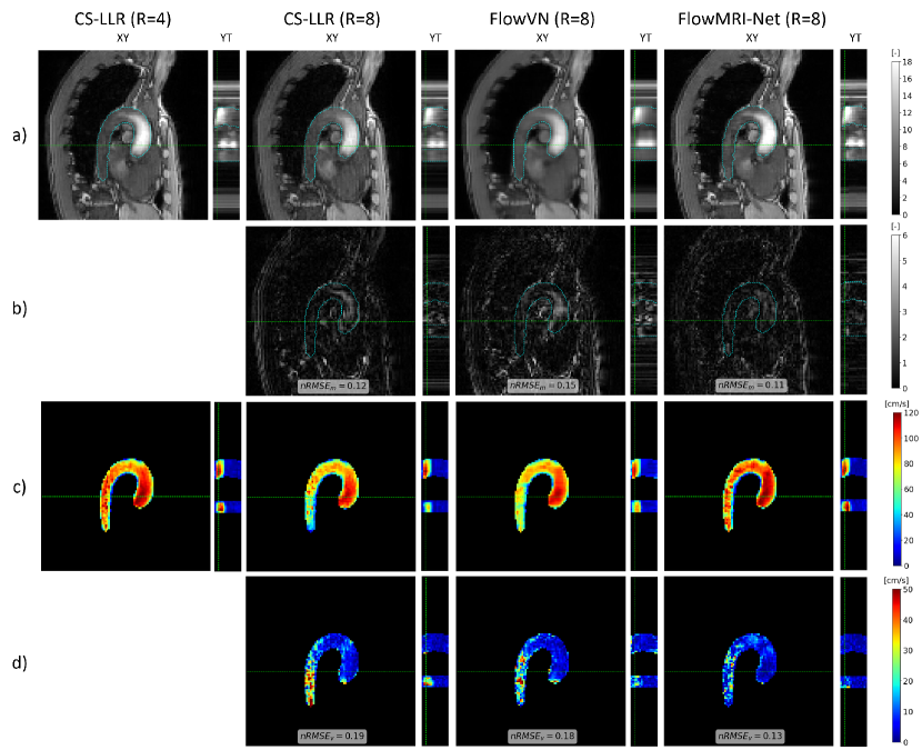
Figure 2: Comparison of reconstruction methods for 8-fold prospectively undersampled aortic data. Image magnitudes (a), absolute image magnitude differences with CS-LLR (R=4) reconstruction (b), velocity magnitudes (c), and velocity magnitude differences with CS-LLR (R=4) reconstruction (d) are shown for a sagittal slice (XY) at peak systole and an AP column over time (YT). Corresponding slice locations and delineation of the aorta are illustrated with green and blue dashed lines, respectively.

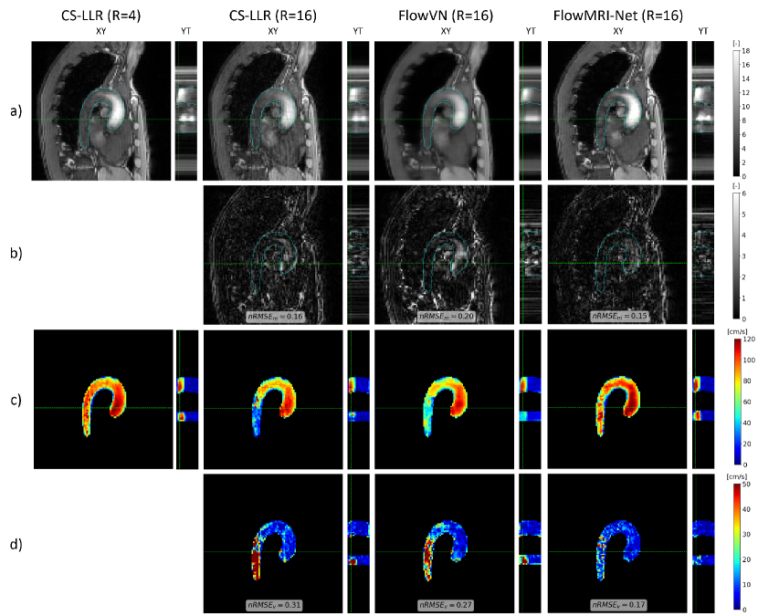
Figure 3: Comparison of reconstruction methods for 16-fold prospectively undersampled aortic data. Image magnitudes (a), absolute image magnitude differences with CS-LLR (R=4) reconstruction (b), velocity magnitudes (c), and velocity magnitude differences with CS-LLR (R=4) reconstruction (d) are shown for a sagittal slice (XY) at peak systole and an AP column over time (YT). Corresponding slice locations and delineation of the aorta are illustrated with green and blue dashed lines, respectively.

The quantitative metrics for aortic reconstructions using CS-LLR, FlowVN, and FlowMRI-Net are summarized in Table 2, with the image magnitudes, velocity magnitudes, and their errors of an exemplary healthy volunteer shown in Fig. 2 and 3 for 8-fold and 16-fold prospective undersampling, respectively. Visual image magnitude quality and $\operatorname{nRMSE_{m}}$ values are similar for CS-LLR and FlowMRI-Net reconstructions for both undersampling factors, whereas FlowVN shows increased spatial and temporal blurring in the image magnitudes. Velocity magnitudes during peak systole are generally underestimated by CS-LLR and FlowVN, particularly in the descending aorta where SNR is lower due to the higher distance to the coils. This underestimation of velocity magnitude is reflected by the inferior $\operatorname{nRMSE_{v}}$ and $\operatorname{mDirErr}$ values of CS-LLR and FlowVN compared to FlowMRI-Net for both undersampling factors.

Table 2: Quantitative metrics for prospectively undersampled aortic reconstructions

Metric	R	CS-LLR	FlowVN	FlowMRI-Net
$\operatorname{nRMSE_{m}}$	8	$\boldsymbol{0.097\pm 0.012}$	$0.148\pm 0.008$	$\boldsymbol{0.097\pm 0.011}$
	16	$\boldsymbol{0.142\pm 0.008}$	$0.193\pm 0.007$	$\boldsymbol{0.142\pm 0.020}$
$\operatorname{nRMSE_{v}}$	8	$0.273\pm 0.080$	$0.244\pm 0.089$	$\boldsymbol{0.189\pm 0.045}$
	16	$0.308\pm 0.066$	$0.302\pm 0.085$	$\boldsymbol{0.239\pm 0.055}$
$\operatorname{mDirErr}$	8	$0.032\pm 0.020$	$0.024\pm 0.016$	$\boldsymbol{0.016\pm 0.008}$
	16	$0.036\pm 0.018$	$0.039\pm 0.025$	$\boldsymbol{0.023\pm 0.015}$

All values are shown as the mean $\pm$ standard deviation, with the lowest
(best) mean values stated in bold

A comparison of peak velocities in the ascending aorta at the level of the right pulmonary artery center between the fully sampled 2D REF and CS-LLR, FlowVN, and FlowMRI-Net reconstructions can be seen in Fig. 4 for undersampling factors R=8 (upper row) and R=16 (bottom row). In FH direction, an underestimation is observed for CS-LLR and FlowVN reconstructions at both undersampling factors whereas FlowMRI-Net accurately captures peak flow. In RL and AP directions, all three reconstruction methods showcase the correct velocity profile, but are relatively noisy.

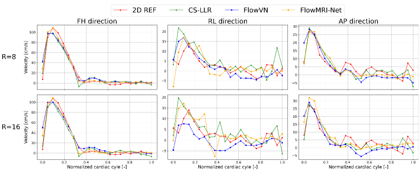
Figure 4: Comparison of peak velocity curves in the ascending aorta. CS-LLR, FlowVN, and FlowMRI-Net reconstructions of prospectively undersampled data, and 2D reference (REF) from fully sampled data acquired during breath-hold.

Reconstructions of a cerebrovascular acquisition at undersampling factors R=8,16, and 24 can be seen in Fig. 5. Visually, the image magnitude of the frame-by-frame reconstructed GRAPPA reference is noisier than the CS-LLR and FlowMRI-Net reconstruction at higher undersampling factors, which is reflected by the lower SNR, particularly in the brain stem furthest away from the coils. Undersampling artifacts appear in the image magnitude for the CS-LLR reconstruction at R=24, with visible underestimation of velocity magnitudes at all undersampling factors, particularly in the left and right internal carotid arteries (ICA) and middle cerebral arteries (MCA). Contrarily, the proposed FlowMRI-Net demonstrates better agreement of velocity magnitudes with the reference GRAPPA reconstruction, even up to the highest undersampling factor (R=24). These observations extend to the peak velocity curves for the left and right MCA and ICA, as seen in Fig. 6, where FlowMRI-Net shows superior agreement with the GRAPPA reconstruction compared to CS-LLR, which tends to underestimate peak velocity magnitudes. CS-LLR underestimates and FlowMRI-Net overestimates the peak velocity in the left and right PCA at all undersampling factors.

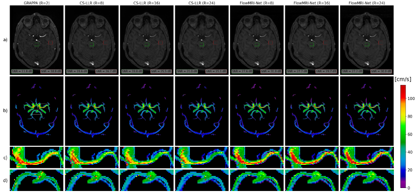
Figure 5: Comparison of reconstruction methods for cerebrovascular data for various undersampling factors. Image magnitudes (a) and maximum intensity projections of velocity magnitudes (b) with zoomed-in sections on the LMCA (c) and LPCA/RPCA (d) are shown, where the SNR has been computed for image magnitude patches in the brain stem (green) and white matter (red).

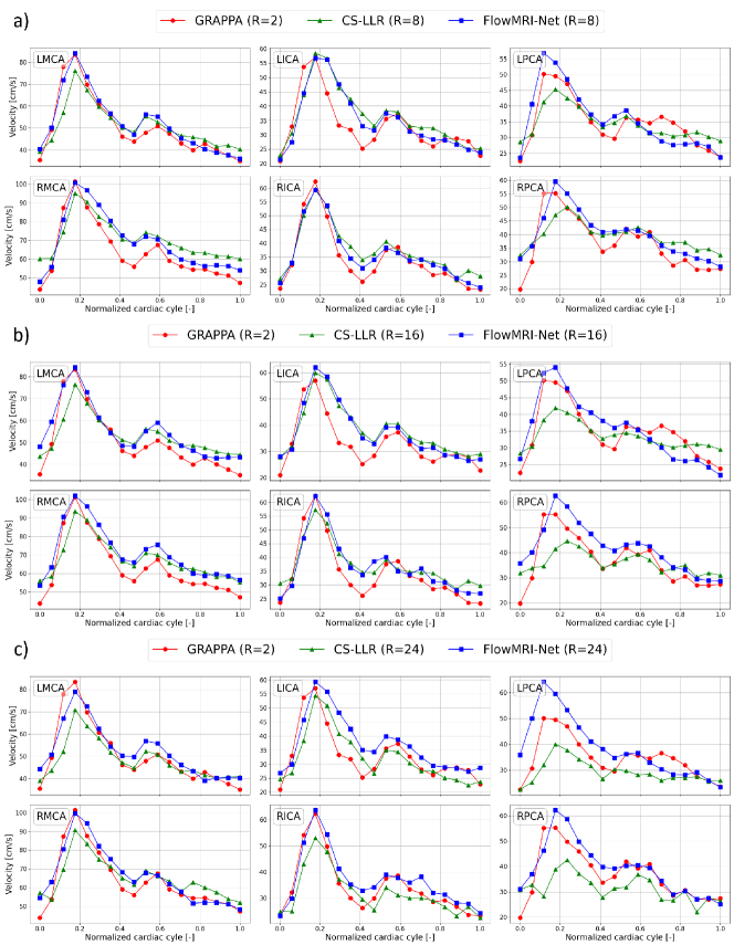
Figure 6: Comparison of peak velocity curves for different vessels in cerebrovascular reconstructions. The spatial coordinate with peak velocity magnitude is determined based on R=8 (a) and is traced for R=16 (b) and R=24 (c), all showing the left and right MCA, ICA, and PCA.

4 Discussion

In this work FlowMRI-Net has been proposed, improving the reconstruction quality over FlowVN and CS-LLR for aortic and cerebrovascular 4D flow MRI and demonstrating its generalizability for cerebrovascular 4D flow MRI, all whilst ensuring clinically feasible reconstruction times. With FlowMRI-Net several improvements compared to FlowVN are introduced: 1) joint reconstruction of all velocity encodings, 2) preservation of the complex representation of the MRI data using a complex-valued network, which was found to be particularly beneficial for phase-focused applications [56], 3) recurrent convolutions that effectively propagate information across unrolling iterations and time, requiring fewer learnable parameters than corresponding 3D convolutions [35], 4) computationally-efficient exact point-wise DC based on unrolled variable splitting optimization [28], and 5) a self-supervised learning strategy that does not rely on the availability or quality of an acquired reference [40].

The superior reconstruction quality of prospectively undersampled aortic 4D flow MRI for R = 8 and 16 was demonstrated both qualitatively (Fig. 2 and 3) and quantitatively (Table 2), with FlowMRI-Net recovering more accurate structural details and hemodynamic features in the image magnitudes and velocity magnitudes compared to CS-LLR and FlowVN reconstructions, resulting in lower $\operatorname{nRMSE_{m}}$ and $\operatorname{mDirErr}$ values. Compared to the fully sampled 2D breath-hold scans, FlowMRI-Net accurately captures peak velocity in FH direction, as opposed to CS-LLR and FlowVN, which both underestimate peak velocity (Fig. 4). Velocities in RL and AP direction remain noisy, which can be explained by the relatively high venc = 150 cm/s compared to the maximum velocities that occur in those two directions for non-pathological flow (vmax ¡ 50 cm/s). The spatiotemporal blurring of FlowVN reconstructions in the work was not observed in the original paper [18], which may be explained by the change in training data and the switch from retrospectively-undersampled data with additional noise as input to prospectively-undersampled data. Also note that in the original paper the CS-LLR was not GPU-accelerated, hence the reported 30-fold increase in reconstruction speed, which does not hold anymore in this work as CS-LLR was also run on a GPU.

In the present study, breathing motion during aortic acquisitions was tracked using the Philips VitalEye camera [29] and only the end-expiration state was considered, which reduces imaging efficiency and prohibits measurement of respiration-resolved flow dynamics (5D flow MRI) [57, 58]. Although the respiratory bins can be reconstructed separately, future work should investigate motion-informed reconstruction to exploit redundancies between breathing states, using learning-based [59] or conventional registration-based [60, 61] motion estimation. Finally, the generalizability to pathological flow dynamics, such as for aortic stenoses, should be investigated.

For cerebrovascular reconstructions, using a two-fold GRAPPA reconstruction as reference, we showed that FlowMRI-Net resulted in improved noise reduction in images magnitudes compared to CS-LLR (Fig. 5), whilst accurately capturing peak velocity magnitudes in the left and right MCA and ICA, even up to an undersampling factor of R=24 (Fig. 6). The velocities in the left and right PCA remain challenging to recover for both CS-LLR and FlowMRI-Net even at R=8 due to the relatively small vessel diameter (2.7 $\pm$ 0.04 mm for the P2 segment that we considered) [62] compared to the spatial acquisition resolution of 0.8 mm $\times$ 0.8 mm $\times$ 0.8 mm. The CS-like k-space sampling implemented on the Siemens system for the cerebrovascular acquisitions was not optimized and may be suboptimal for FlowMRI-Net. In brief, the sampling pattern has non-random patterns that cause higher lateral peaks in the corresponding point-spread function (i.e. higher coherence) compared to truly pseudo-random sampling, resulting in structured undersampling artifacts that are undesirable in our context [11]. Moreover, the corners of k-space, which are less critical, were sampled relatively densely; a proper elliptical shutter can increase imaging efficiency. Furthermore, it is currently unclear whether incoherent/complementary sampling between velocity-encodings is desirable for FlowMRI-Net reconstructions. Namely, such incoherence may be beneficial when exploiting redundancies between velocity encodings for the joint reconstruction [32]. On the other hand, coherence may be beneficial because any undersampling artifacts that remain after reconstruction would be the same for the velocity encodings and hence would disappear when computing phase differences. Future work should investigate a more optimal sampling pattern, possibly incorporating it in the optimization loop for an anatomy-specific sampling [63, 64]. Finally, a larger cohort including patients should be considered for further validation and proof of generalizability to pathological flow dynamics, such as an intracranial aneurysm, should be investigated.

5 Conclusion

This paper presented FlowMRI-Net, a generalizable deep learning-based physics-driven reconstruction network for reconstructing from highly undersampled 4D flow MRI in clinically feasible reconstruction times as exemplarily demonstrated for aortic and cerebrovascular applications. Since FlowMRI-Net is computationally efficient and does not require a reference for training, it can easily be extended to other applications where reference data is not available. It is anticipated that FlowMRI-Net conduces the use of accelerated 4D flow MRI in a clinical setting.

References

- [1] M. Markl, A. Frydrychowicz, S. Kozerke, M. Hope, and O. Wieben, “4d flow mri,” Journal of Magnetic Resonance Imaging, vol. 36, no. 5, pp. 1015–1036, 2012.
- [2] A. Frydrychowicz, A. F. Stalder, M. F. Russe, J. Bock, S. Bauer, A. Harloff, A. Berger, M. Langer, J. Hennig, and M. Markl, “Three-dimensional analysis of segmental wall shear stress in the aorta by flow-sensitive four-dimensional-MRI,” Journal of Magnetic Resonance Imaging, vol. 30, no. 1, pp. 77–84, 2009.
- [3] J. Bock, A. Frydrychowicz, R. Lorenz, D. Hirtler, A. J. Barker, K. M. Johnson, R. Arnold, H. Burkhardt, J. Hennig, and M. Markl, “In vivo noninvasive 4D pressure difference mapping in the human aorta: Phantom comparison and application in healthy volunteers and patients,” Magnetic Resonance in Medicine, vol. 66, no. 4, pp. 1079–1088, 2011.
- [4] M. Markl, W. Wallis, S. Brendecke, J. Simon, A. Frydrychowicz, and A. Harloff, “Estimation of global aortic pulse wave velocity by flow-sensitive 4D MRI,” Magnetic Resonance in Medicine, vol. 63, no. 6, pp. 1575–1582, 2010.
- [5] M. Markl, S. Schnell, C. Wu, E. Bollache, K. Jarvis, A. J. Barker, J. D. Robinson, and C. K. Rigsby, “Advanced flow MRI: emerging techniques and applications,” Clinical Radiology, vol. 71, no. 8, pp. 779–795, Aug. 2016.
- [6] P. Dyverfeldt, M. Bissell, A. J. Barker, A. F. Bolger, C.-J. Carlhäll, T. Ebbers, C. J. Francios, A. Frydrychowicz, J. Geiger, D. Giese et al., “4d flow cardiovascular magnetic resonance consensus statement,” Journal of Cardiovascular Magnetic Resonance, vol. 17, no. 1, p. 72, 2015.
- [7] M. M. Bissell, F. Raimondi, L. Ait Ali, B. D. Allen, A. J. Barker, A. Bolger, N. Burris, C.-J. Carhäll, J. D. Collins, T. Ebbers, C. J. Francois, A. Frydrychowicz, P. Garg, J. Geiger, H. Ha, A. Hennemuth, M. D. Hope, A. Hsiao, K. Johnson, S. Kozerke, L. E. Ma, M. Markl, D. Martins, M. Messina, T. H. Oechtering, P. van Ooij, C. Rigsby, J. Rodriguez-Palomares, A. A. W. Roest, A. Roldán-Alzate, S. Schnell, J. Sotelo, M. Stuber, A. B. Syed, J. Töger, R. van der Geest, J. Westenberg, L. Zhong, Y. Zhong, O. Wieben, and P. Dyverfeldt, “4D Flow cardiovascular magnetic resonance consensus statement: 2023 update,” Journal of Cardiovascular Magnetic Resonance, vol. 25, no. 1, p. 40, Feb. 2023.
- [8] K. P. Pruessmann, M. Weiger, M. B. Scheidegger, and P. Boesiger, “Sense: sensitivity encoding for fast mri,” Magnetic Resonance in Medicine: An Official Journal of the International Society for Magnetic Resonance in Medicine, vol. 42, no. 5, pp. 952–962, 1999.
- [9] M. A. Griswold, P. M. Jakob, R. M. Heidemann, M. Nittka, V. Jellus, J. Wang, B. Kiefer, and A. Haase, “Generalized autocalibrating partially parallel acquisitions (GRAPPA),” Magnetic Resonance in Medicine, vol. 47, no. 6, pp. 1202–1210, 2002.
- [10] D. K. Sodickson and W. J. Manning, “Simultaneous acquisition of spatial harmonics (SMASH): Fast imaging with radiofrequency coil arrays,” Magnetic Resonance in Medicine, vol. 38, no. 4, pp. 591–603, 1997.
- [11] M. Lustig, D. Donoho, and J. M. Pauly, “Sparse MRI: The application of compressed sensing for rapid MR imaging,” Magnetic Resonance in Medicine, vol. 58, no. 6, pp. 1182–1195, 2007.
- [12] J. Tsao, P. Boesiger, and K. P. Pruessmann, “k-t BLAST and k-t SENSE: Dynamic MRI with high frame rate exploiting spatiotemporal correlations,” Magnetic Resonance in Medicine, vol. 50, no. 5, pp. 1031–1042, 2003.
- [13] H. Pedersen, S. Kozerke, S. Ringgaard, K. Nehrke, and W. Y. Kim, “k-t PCA: Temporally constrained k-t BLAST reconstruction using principal component analysis,” Magnetic Resonance in Medicine, vol. 62, no. 3, pp. 706–716, 2009.
- [14] D. Liang, J. Cheng, Z. Ke, and L. Ying, “Deep MRI Reconstruction: Unrolled Optimization Algorithms Meet Neural Networks,” Jul. 2019.
- [15] B. Zhu, J. Z. Liu, S. F. Cauley, B. R. Rosen, and M. S. Rosen, “Image reconstruction by domain-transform manifold learning,” Nature, vol. 555, no. 7697, pp. 487–492, Mar. 2018.
- [16] K. Hammernik, T. Klatzer, E. Kobler, M. P. Recht, D. K. Sodickson, T. Pock, and F. Knoll, “Learning a Variational Network for Reconstruction of Accelerated MRI Data,” Apr. 2017.
- [17] K. Hammernik, T. Küstner, B. Yaman, Z. Huang, D. Rueckert, F. Knoll, and M. Akçakaya, “Physics-Driven Deep Learning for Computational Magnetic Resonance Imaging: Combining physics and machine learning for improved medical imaging,” IEEE Signal Processing Magazine, vol. 40, no. 1, pp. 98–114, Jan. 2023.
- [18] V. Vishnevskiy, J. Walheim, and S. Kozerke, “Deep variational network for rapid 4D flow MRI reconstruction,” Nature Machine Intelligence, vol. 2, no. 4, pp. 228–235, Apr. 2020.
- [19] F. M. Callaghan, R. Kozor, A. G. Sherrah, M. Vallely, D. Celermajer, G. A. Figtree, and S. M. Grieve, “Use of multi-velocity encoding 4D flow MRI to improve quantification of flow patterns in the aorta,” Journal of Magnetic Resonance Imaging, vol. 43, no. 2, pp. 352–363, 2016.
- [20] S. Schnell, S. A. Ansari, C. Wu, J. Garcia, I. G. Murphy, O. A. Rahman, A. A. Rahsepar, M. Aristova, J. D. Collins, J. C. Carr, and M. Markl, “Accelerated dual-venc 4D flow MRI for neurovascular applications,” Journal of Magnetic Resonance Imaging, vol. 46, no. 1, pp. 102–114, 2017.
- [21] J. Walheim, H. Dillinger, and S. Kozerke, “Multipoint 5D flow cardiovascular magnetic resonance - accelerated cardiac- and respiratory-motion resolved mapping of mean and turbulent velocities,” Journal of Cardiovascular Magnetic Resonance, vol. 21, no. 1, p. 42, Jul. 2019.
- [22] B. Yaman, S. A. H. Hosseini, S. Moeller, J. Ellermann, K. Uğurbil, and M. Akçakaya, “Self-supervised learning of physics-guided reconstruction neural networks without fully sampled reference data,” Magnetic Resonance in Medicine, vol. 84, no. 6, pp. 3172–3191, 2020.
- [23] M. Acar, T. Çukur, and İ. Öksüz, “Self-supervised dynamic mri reconstruction,” in Machine Learning for Medical Image Reconstruction: 4th International Workshop, MLMIR 2021, Held in Conjunction with MICCAI 2021, Strasbourg, France, October 1, 2021, Proceedings 4. Springer, 2021, pp. 35–44.
- [24] M. Blumenthal, C. Fantinato, C. Unterberg-Buchwald, M. Haltmeier, X. Wang, and M. Uecker, “Self-supervised learning for improved calibrationless radial MRI with NLINV-Net,” Magnetic Resonance in Medicine, 2024.
- [25] O. B. Demirel, B. Yaman, C. Shenoy, S. Moeller, S. Weingärtner, and M. Akçakaya, “Signal intensity informed multi-coil encoding operator for physics-guided deep learning reconstruction of highly accelerated myocardial perfusion CMR,” Magnetic Resonance in Medicine, vol. 89, no. 1, pp. 308–321, 2023.
- [26] B. Yaman, C. Shenoy, Z. Deng, S. Moeller, H. El-Rewaidy, R. Nezafat, and M. Akçakaya, “Self-Supervised Physics-Guided Deep Learning Reconstruction for High-Resolution 3D LGE CMR,” in 2021 IEEE 18th International Symposium on Biomedical Imaging (ISBI), Apr. 2021, pp. 100–104.
- [27] N. J. Pelc, M. A. Bernstein, A. Shimakawa, and G. H. Glover, “Encoding strategies for three-direction phase-contrast MR imaging of flow,” Journal of Magnetic Resonance Imaging, vol. 1, no. 4, pp. 405–413, 1991.
- [28] J. Duan, J. Schlemper, C. Qin, C. Ouyang, W. Bai, C. Biffi, G. Bello, B. Statton, D. P. O’Regan, and D. Rueckert, “VS-Net: Variable Splitting Network for Accelerated Parallel MRI Reconstruction,” in Medical Image Computing and Computer Assisted Intervention – MICCAI 2019, D. Shen, T. Liu, T. M. Peters, L. H. Staib, C. Essert, S. Zhou, P.-T. Yap, and A. Khan, Eds. Cham: Springer International Publishing, 2019, pp. 713–722.
- [29] L. Gottwald, C. Blanken, J. Tourais, J. Smink, R. Planken, S. Boekholdt, L. Meijboom, B. Coolen, G. Strijkers, A. Nederveen, and P. Ooij, “Retrospective Camera‐Based Respiratory Gating in Clinical Whole‐Heart 4D Flow MRI,” Journal of Magnetic Resonance Imaging, vol. 54, Mar. 2021.
- [30] P. Ehses, “pehses/twixtools,” May 2024.
- [31] M. Uecker, J. I. Tamir, F. Ong, and M. Lustig, “The BART toolbox for computational magnetic resonance imaging,” in Proc Intl Soc Magn Reson Med, vol. 24, 2016, p. 1.
- [32] D. Polak, S. Cauley, B. Bilgic, E. Gong, P. Bachert, E. Adalsteinsson, and K. Setsompop, “Joint multi-contrast variational network reconstruction (jVN) with application to rapid 2D and 3D imaging,” Magnetic Resonance in Medicine, vol. 84, no. 3, pp. 1456–1469, 2020.
- [33] G. S. Roberts, C. A. Hoffman, L. A. Rivera-Rivera, S. E. Berman, L. B. Eisenmenger, and O. Wieben, “Automated hemodynamic assessment for cranial 4D flow MRI,” Magnetic Resonance Imaging, vol. 97, pp. 46–55, Apr. 2023.
- [34] M. A. Bernstein and Y. Ikezaki, “Comparison of phase-difference and complex-difference processing in phase-contrast MR angiography,” Journal of Magnetic Resonance Imaging, vol. 1, no. 6, pp. 725–729, 1991.
- [35] C. Qin, J. Schlemper, J. Caballero, A. N. Price, J. V. Hajnal, and D. Rueckert, “Convolutional Recurrent Neural Networks for Dynamic MR Image Reconstruction,” IEEE Transactions on Medical Imaging, vol. 38, no. 1, pp. 280–290, Jan. 2019.
- [36] X. Glorot, A. Bordes, and Y. Bengio, “Deep Sparse Rectifier Neural Networks,” in Proceedings of the Fourteenth International Conference on Artificial Intelligence and Statistics. JMLR Workshop and Conference Proceedings, Jun. 2011, pp. 315–323.
- [37] M. Arjovsky, A. Shah, and Y. Bengio, “Unitary Evolution Recurrent Neural Networks,” in Proceedings of The 33rd International Conference on Machine Learning. PMLR, Jun. 2016, pp. 1120–1128.
- [38] T. Chen, B. Xu, C. Zhang, and C. Guestrin, “Training Deep Nets with Sublinear Memory Cost,” Apr. 2016.
- [39] M. Rhu, N. Gimelshein, J. Clemons, A. Zulfiqar, and S. W. Keckler, “vDNN: Virtualized deep neural networks for scalable, memory-efficient neural network design,” in 2016 49th Annual IEEE/ACM International Symposium on Microarchitecture (MICRO), 2016, pp. 1–13.
- [40] B. Yaman, H. Gu, S. A. H. Hosseini, O. B. Demirel, S. Moeller, J. Ellermann, K. Uğurbil, and M. Akçakaya, “Multi-mask self-supervised learning for physics-guided neural networks in highly accelerated magnetic resonance imaging,” NMR in Biomedicine, vol. 35, no. 12, p. e4798, 2022.
- [41] C. Shorten and T. M. Khoshgoftaar, “A survey on Image Data Augmentation for Deep Learning,” Journal of Big Data, vol. 6, no. 1, p. 60, Jul. 2019.
- [42] D. P. Kingma and J. Ba, “Adam: A Method for Stochastic Optimization,” Jan. 2017.
- [43] A. Paszke, S. Gross, F. Massa, A. Lerer, J. Bradbury, G. Chanan, T. Killeen, Z. Lin, N. Gimelshein, L. Antiga, A. Desmaison, A. Kopf, E. Yang, Z. DeVito, M. Raison, A. Tejani, S. Chilamkurthy, B. Steiner, L. Fang, J. Bai, and S. Chintala, “PyTorch: An Imperative Style, High-Performance Deep Learning Library,” in Advances in Neural Information Processing Systems, vol. 32. Curran Associates, Inc., 2019.
- [44] W. Falcon and The PyTorch Lightning team, “PyTorch Lightning,” Mar. 2019.
- [45] T. Zhang, J. M. Pauly, and I. R. Levesque, “Accelerating parameter mapping with a locally low rank constraint,” Magnetic Resonance in Medicine, vol. 73, no. 2, pp. 655–661, 2015.
- [46] C. Santelli, M. Loecher, J. Busch, O. Wieben, T. Schaeffter, and S. Kozerke, “Accelerating 4D flow MRI by exploiting vector field divergence regularization,” Magnetic Resonance in Medicine, vol. 75, no. 1, pp. 115–125, 2016.
- [47] P. A. Yushkevich, J. Piven, H. C. Hazlett, R. G. Smith, S. Ho, J. C. Gee, and G. Gerig, “User-guided 3D active contour segmentation of anatomical structures: Significantly improved efficiency and reliability,” NeuroImage, vol. 31, no. 3, pp. 1116–1128, Jul. 2006.
- [48] F. Isensee, P. F. Jaeger, S. A. Kohl, J. Petersen, and K. H. Maier-Hein, “nnU-Net: a self-configuring method for deep learning-based biomedical image segmentation,” Nature methods, vol. 18, no. 2, pp. 203–211, 2021.
- [49] X. Liu, F. Pu, Y. Fan, X. Deng, D. Li, and S. Li, “A numerical study on the flow of blood and the transport of LDL in the human aorta: the physiological significance of the helical flow in the aortic arch,” American Journal of Physiology-Heart and Circulatory Physiology, vol. 297, no. 1, pp. H163–H170, Jul. 2009.
- [50] B. C. Lowekamp, D. T. Chen, L. Ibanez, and D. Blezek, “The Design of SimpleITK,” Frontiers in Neuroinformatics, vol. 7, Dec. 2013.
- [51] N. J. Tustison, B. B. Avants, P. A. Cook, Y. Zheng, A. Egan, P. A. Yushkevich, and J. C. Gee, “N4ITK: Improved N3 Bias Correction,” IEEE Transactions on Medical Imaging, vol. 29, no. 6, pp. 1310–1320, Jun. 2010.
- [52] M. A. Bernstein, X. J. Zhou, J. A. Polzin, K. F. King, A. Ganin, N. J. Pelc, and G. H. Glover, “Concomitant gradient terms in phase contrast mr: analysis and correction,” Magnetic resonance in medicine, vol. 39, no. 2, pp. 300–308, 1998.
- [53] C. Fischer, J. Wetzl, T. Schaeffter, and D. Giese, “Fully automated background phase correction using M-estimate SAmple consensus (MSAC)—Application to 2D and 4D flow,” Magnetic Resonance in Medicine, vol. 88, no. 6, pp. 2709–2717, 2022.
- [54] M. Loecher, E. Schrauben, K. M. Johnson, and O. Wieben, “Phase unwrapping in 4D MR flow with a 4D single-step laplacian algorithm,” Journal of Magnetic Resonance Imaging, vol. 43, no. 4, pp. 833–842, 2016.
- [55] P. Dirix, L. Jacobs, and S. Kozerke, “4Dflow-unwrap: A collection of python-based phase unwrapping algorithms,” in Proc Intl Soc Mag Reson Med, 2024.
- [56] E. Cole, J. Cheng, J. Pauly, and S. Vasanawala, “Analysis of deep complex-valued convolutional neural networks for MRI reconstruction and phase-focused applications,” Magnetic Resonance in Medicine, vol. 86, no. 2, pp. 1093–1109, 2021.
- [57] J. Walheim, H. Dillinger, A. Gotschy, and S. Kozerke, “5D Flow Tensor MRI to Efficiently Map Reynolds Stresses of Aortic Blood Flow In-Vivo,” Scientific Reports, vol. 9, no. 1, p. 18794, Dec. 2019.
- [58] L. E. Ma, J. Yerly, D. Piccini, L. Di Sopra, C. W. Roy, J. C. Carr, C. K. Rigsby, D. Kim, M. Stuber, and M. Markl, “5D Flow MRI: A Fully Self-gated, Free-running Framework for Cardiac and Respiratory Motion–resolved 3D Hemodynamics,” Radiology: Cardiothoracic Imaging, vol. 2, no. 6, p. e200219, Dec. 2020.
- [59] J. Pan, W. Huang, D. Rueckert, T. Küstner, and K. Hammernik, “Motion-Compensated MR CINE Reconstruction With Reconstruction-Driven Motion Estimation,” IEEE Transactions on Medical Imaging, vol. 43, no. 7, pp. 2420–2433, Jul. 2024.
- [60] P. G. Batchelor, D. Atkinson, P. Irarrazaval, D. L. G. Hill, J. Hajnal, and D. Larkman, “Matrix description of general motion correction applied to multishot images,” Magnetic Resonance in Medicine, vol. 54, no. 5, pp. 1273–1280, 2005.
- [61] V. Vishnevskiy, T. Gass, G. Szekely, C. Tanner, and O. Goksel, “Isotropic Total Variation Regularization of Displacements in Parametric Image Registration,” IEEE Transactions on Medical Imaging, vol. 36, no. 2, pp. 385–395, Feb. 2017.
- [62] S. A. Gunnal, M. S. Farooqui, and R. N. Wabale, “Study of Posterior Cerebral Artery in Human Cadaveric Brain,” Anatomy Research International, vol. 2015, p. 681903, 2015.
- [63] H. K. Aggarwal and M. Jacob, “J-MoDL: Joint Model-Based Deep Learning for Optimized Sampling and Reconstruction,” IEEE Journal of Selected Topics in Signal Processing, vol. 14, no. 6, pp. 1151–1162, Oct. 2020.
- [64] C. D. Bahadir, A. Q. Wang, A. V. Dalca, and M. R. Sabuncu, “Deep-Learning-Based Optimization of the Under-Sampling Pattern in MRI,” IEEE Transactions on Computational Imaging, vol. 6, pp. 1139–1152, 2020.