Hybrid LLM-DDQN based Joint Optimization of V2I Communication and Autonomous Driving

Abstract

Large language models (LLMs) have received considerable interest recently due to their outstanding reasoning and comprehension capabilities. This work explores applying LLMs to vehicular networks, aiming to jointly optimize vehicle-to-infrastructure (V2I) communications and autonomous driving (AD) policies. We deploy LLMs for AD decision-making to maximize traffic flow and avoid collisions for road safety, and a double deep Q-learning algorithm (DDQN) is used for V2I optimization to maximize the received data rate and reduce frequent handovers. In particular, for LLM-enabled AD, we employ the Euclidean distance to identify previously explored AD experiences, and then LLMs can learn from past good and bad decisions for further improvement. Then, LLM-based AD decisions will become part of states in V2I problems, and DDQN will optimize the V2I decisions accordingly. After that, the AD and V2I decisions are iteratively optimized until convergence. Such an iterative optimization approach can better explore the interactions between LLMs and conventional reinforcement learning techniques, revealing the potential of using LLMs for network optimization and management. Finally, the simulations demonstrate that our proposed hybrid LLM-DDQN approach outperforms the conventional DDQN algorithm, showing faster convergence and higher average rewards.

I Introduction

Large Language Models (LLMs) are emerging as a promising technique to address a wide range of downstream tasks such as classification, prediction, and optimization [1]. Conventional algorithms, such as convex optimization and reinforcement learning (RL), experience scalability issues. For example, RL usually experiences a large number of iterations and well-known low sampling efficiency issues, and convex optimization requires dedicated problem transformation for convexity. By contrast, existing studies have shown that LLM-inspired optimization, i.e., in-context learning-based approaches, have several unique advantages: 1) LLMs can perform in-context learning without any extra model training or parameter fine-tuning, saving considerable human effort; 2) LLM-based in-context optimization can quickly scale to new tasks or objectives by simply adjusting the prompts, thus enable rapid adaptation to various communication environments; 3) LLMs can provide reasonable explanations for their optimization decisions, helping human understanding complex network systems. With these appealing features, LLMs have great potential for handling optimization problems.

On the other hand, the envisioned 6G networks will observe short channel coherence time (due to higher transmission frequencies and narrow beams) and stringent requirements on the quality of network services, calling for faster response time and higher intelligence. For example, vehicle-to-infrastructure (V2I) communication is closely related to vehicle’s driving behaviours, e.g., frequent acceleration and deceleration can result in extra handovers (HOs) and can even result in V2I connection outages (if not handled on a timely basis) [2]. As a result, jointly optimizing V2I communication and autonomous driving (AD) policies is critical. Such integration of V2I and AD also aligns with the 6G usage scenarios defined in International Mobile Telecommunications-2030 (IMT-2030) by the International Telecommunication Union [3].

LLM-based AD has attracted significant research interest, and existing studies have leveraged LLM’s reasoning capabilities to enable decision-making [4] and leading human-like AD behaviours [5]. While a couple of research works [5, 4] considered LLMs for AD, the problem of jointly optimizing V2I communication and AD policies has only been solved using traditional RL techniques [2, 6]. Therefore, the performance gains of using LLM in solving the joint V2I connectivity and AD problem are unexplored.

To this end, this article aims to investigate the benefits of LLMs in solving the joint optimization of V2I communication and AD policies. Since most existing LLMs, such as GPT and Llama, are pretrained for general domain purposes, we propose a hybrid LLM-DDQN based iterative solution. In particular, we first employ LLMs for AD decision-making, aiming to maximize speed, reduce lane changes, and collisions. Using the pre-trained real-world knowledge, LLMs can better understand complicated road environments and quickly make AD decisions. We introduce the language-based task description, example design and distance-based selection, enabling LLMs to explore and learn from previous experience. After that, the AD decision will be used by the double deep Q-Networks (DDQN) for V2I optimization, which is designed to improve data rates with fewer handovers. The whole problem will be iteratively optimized until convergence. Our simulation results show that the proposed LLM-based method has higher learning efficiency and faster convergence than baselines. Here, we select DDQN for V2I optimization as we note DDWN’s superior performance compared to LLMs. Also, the performance of DDQN is well-established and has been demonstrated in many existing studies[2, 6].

Figure 1: Hybrid LLM-DDQN Framework in the RF-THz-Highway Environment

II System Model and MDP Definitions

This section will introduce the considered system model for AD and V2I connectivity as well as their corresponding Markov decision processes (MDPs). MDP is a very useful approach to define optimization tasks, therefore, we modeled this problem using an MDP.

II-A V2I and AD System Models

As shown in Figure 1, we consider a downlink network consisting of $N_{R}$ RF base stations (RBSs) and $N_{T}$ THz base stations (TBSs) in a multi-vehicle environment. Specifically, from the V2I communication perspective, we aim to maximize the V2I data rate and minimize handovers. From the transportation perspective, road safety must be considered, which will optimize velocity and minimize collisions.

We assume there are $M_{1}$ autonomous vehicles (AVs) receiving data from roadside BSs [2]. Each AV is associated with a single BS (either RBS or TBS). The AVs’ onboard units collect real-time data from the VNet, including neighboring vehicles’ velocity, acceleration, and lane positions. The signal-to-interference-plus-noise ratio (SINR) for the $j$-th AV from BS $i$ is modelled as in [2]:

$${}\mathrm{SINR}^{\mathrm{RF}}_{ij}=\frac{P_{R}^{\mathrm{tx}}\>G_{R}^{\mathrm{tx}}\>G_{R}^{\mathrm{rx}}\left(\frac{c}{4\pi f_{R}}\right)^{2}H_{i}}{r_{ij}^{\alpha}\left(\sigma^{2}+I_{R_{j}}\right)},$$ (1)

where $P_{R}^{\mathrm{tx}},G_{R}^{\mathrm{tx}},G_{R}^{\mathrm{rx}},c,f_{R}$, and $\alpha$ denote the transmit power of the RBSs, antenna transmitting gain, antenna receiving gain, speed of light, RF carrier frequency (in GHz), and path-loss exponent, respectively. Note that $r_{ij}={(d_{ij}^{2}+h_{ij}^{2})}^{1/2},$ where $d_{ij}$ is the 2D distance between the $j$-th AV and $i$-th BS and $h_{ij}$ is the transmit antenna height. In addition, $H_{i}$ is the exponentially distributed channel fading power observed at the $j$-th AV from the $i$-th RBS, $\sigma^{2}$ is the power of thermal noise at the receiver, $I_{R_{j}}$ is the cumulative interference at $j$-th AV from the interfering RBSs. The SINR in THz network for a given $j$-th AV can be modelled as follows [7]:

where $G_{T}^{\text{tx}},G_{T}^{\text{rx}},P_{T}^{\text{tx}},f_{T},\text{ and }K_{a}(f_{T})$ represent the transmit antenna gain of the TBS, the receiving antenna gain of the TBS, the transmit power of the TBS, the THz carrier frequency, and the molecular absorption coefficient of the transmission medium, respectively. We assume all AVs are equipped with a single antenna, and beam alignment techniques ensure the AV’s receiving beam aligns with the associated TBS’s transmitting beam. The alignment of the main lobes of user and interfering TBSs occurs with probability $q$, and interference is calculated accordingly [7]. The available bandwidth for each RBS and TBS is denoted as $W_{R}$ and $W_{T}$, respectively. The data rate of each AV-BS link is computed as $R_{ij}=W_{j}\log_{2}(1+\mathrm{SINR}_{ij})$.

In the subsequent subsections, we formulate the AD and V2I optimization problems into two MDPs, since MDP is a very useful approach to define optimization tasks. These MDPs will be further used for LLMs to understand the AD tasks, and DDQN algorithms for V2I decision-making, respectively.

II-B Autonomous Driving MDPs

II-B1 States

The transportation state-space consists of kinematics-related features of AVs, represented as $M_{1}\times F_{\mathrm{AD}}$ array, where $F_{\mathrm{AD}}=\{x^{j},y^{j},v^{j},\psi^{j}\}$ for $j\in[1,M_{1}]$ describes the $j$-th AV’s coordinates $(x^{j},y^{j})$, velocity $v^{j}$, and heading $\psi^{j}$. We model $M_{1}$ target AVs and $M_{2}$ surrounding AVs. The aggregated state space $\mathcal{S}^{\mathrm{AD}}$ at time step $t$ is:

$$\mathcal{S}^{\mathrm{AD}}=[\mathbf{x}^{j},\mathbf{y}^{j},\mathbf{v}^{j},\boldsymbol{\psi}^{j}]$$

II-B2 Actions

At each time step $t$, AV $j$ selects an autonomous driving action $a^{\rm AD}_{t}\in\mathcal{A}_{\rm AD}$, where the driving action space is $\mathcal{A}_{\rm AD}=\{a^{\rm AD}_{1},\ldots,a^{\rm AD}_{5}\}$, representing acceleration, maintaining current lane, deceleration, lane change to left, and lane change to right.

II-B3 Rewards

The transportation reward is defined as:

$$r^{\mathrm{j,AD}}_{t}=c_{1}\left(\frac{v^{j}_{t}-v_{\min}}{v_{\max}-v_{\min}}\right)-c_{2}\delta_{2}+c_{3}\delta_{3}+c_{4}\delta_{4},$$ (3)

where $v^{j}_{t}$ is the AV’s velocity, and $\delta_{2},\delta_{3},\delta_{4}$ represent collision, right-lane, and off-road indicators, respectively. The weights $c_{1}$ and $c_{2}$ adjust the AD reward by incorporating a collision penalty. Specifically, $c_{1}$ scales the reward received when driving at full speed. The reward decreases linearly as the speed decreases, reaching zero at the lowest speed. $c_{2}$ is the collision penalty, which is significantly larger than the other coefficients. To encourage the AV to drive on the rightmost lanes, $c_{3}$ decreases linearly as the AV deviates from the rightmost lane, reaching zero for other lanes. $c_{4}$ is the on-road reward factor, which penalizes the AV for driving off the highway.

II-C Vehicle-to-Infrastructure MDPs

We assume each RBS and TBS can support a maximum of $Q_{R}$ and $Q_{T}$ AVs, respectively [6]. The connection is satisfactory if the SINR can meet or exceed a threshold $\gamma_{th}$. The number of AVs that each BS can serve at a given time is denoted by $n_{i}$. As AVs move along the road, they switch BS connections when $\mathrm{SINR}_{ij}<\gamma_{th}$. Frequent HOs will reduce the data rate due to HO latency. To mitigate this, a HO penalty $\mu$ is introduced, with a higher penalty for TBSs and a lower one for RBSs. The weighted data rate between BS $i$ and AV $j$ is modeled as follows:

$$\text{WR}_{ij}=\frac{R_{ij}}{\min\left(Q_{i},n_{i}\right)}(1-\mu),$$ (4)

where $Q_{i}=\{Q_{R},Q_{T}\}$ in terms of BS $i$ type, $n_{i}$ is the number of existing users on BS $i$. Given these settings, following is the MDP formulation.

II-C1 States

The telecommunication V2I state space is defined as: $\mathcal{S}^{\mathrm{V2I}}=[\mathbf{n}_{R}^{j},\mathbf{n}_{T}^{j},\mathbf{a}^{j,\mathrm{AD}}],$ where $\mathbf{n}_{R}^{j}$ and $\mathbf{n}_{T}^{j}$ represent the numbers of reachable RBSs and TBSs for AV $j$, and $\mathbf{a}^{j,\mathrm{AD}}$ is the transportation action formerly produced by LLM.

II-C2 Actions

At each time step $t$, AV $j$ selects a V2I action $a^{\rm tele}_{t}\in\mathcal{A}_{\rm tele}$, where $\mathcal{A}_{\rm tele}=\{a^{\rm tele}_{1},a^{\rm tele}_{2},a^{\rm tele}_{3}\}$. In $a^{\rm tele}_{1}$, the AV $j$ selects a BS $i$ maximizing the weighted rate metric $\text{WR}_{ij}$. In $a^{\rm tele}_{2}$, the AV selects a BS with maximum $\text{WR}_{ij}$, with $\mu=0$ if $Q_{i}\geq n_{i}(t)$, otherwise selecting the next available BS. In $a^{\rm tele}_{3}$, the AV connects to the BS with the highest data rate $R_{ij}$.

II-C3 Rewards

Given $\xi^{j}_{t},\text{WR}_{i^{*},j,t}$ are the HO rate and the weighted data rate,respectively. The V2I reward is defined as:

$$r^{\mathrm{j,V2I}}_{t}=\text{WR}_{i^{*},j,t}\left(1-\min(1,\xi^{j}_{t})\right),$$ (5)

III Hybrid LLM-DDQN based Dual Objective Optimization Algorithm

As shown in Fig. 1, we propose an iterative optimization framework to integrate LLMs and DDQN to address joint AD and V2I decision-making. The first stage involves utilizing LLMs to make autonomous driving decisions. Then the second stage incorporates the DDQN algorithm, focusing on V2I decisions of selecting proper BSs. In the context of LLM in-context learning [1, 8, 9], we integrated the textual context into the formatted model. Our problem is divided into transportation and V2I steps.

$$D_{task}^{\mathrm{AD}}\times\mathcal{E}_{t}\times\mathcal{S}^{\mathrm{AD}}_{t}\times\mathcal{LLM}\Rightarrow a_{t}^{\mathrm{AD}},$$ (6)

$$\mathcal{S}^{\mathrm{V2I}}_{t}\times a_{t}^{\mathrm{AD}}\times\mathcal{DDQN}\Rightarrow a_{t}^{\mathrm{V2I}},$$ (7)

Here equation (6) shows the decision-making process of LLMs. In particular, $D_{task}^{\mathrm{AD}}$ represents the transportation task descriptions, providing fundamental task information to the LLM, i.e., goals and decision variables. $\mathcal{E}_{t}$ is the set of examples at time $t$, serving as demonstrations for LLMs to learn from, including both positive and negative examples. $\mathcal{S}^{\mathrm{AD}}_{t}$ indicates the current environment state which is associated with the target task. Then $\mathcal{LLM}$ refers to pre-trained LLM models, and $a_{t}^{\mathrm{AD}}$ is the transport decision as we defined in Section II-C. Meanwhile, equation (6) shows the decision-making of DDQN, including communication network state $\mathcal{S}^{\mathrm{V2I}}_{t}$, DDQN model $\mathcal{DDQN}$ and network decision $a_{t}^{\mathrm{V2I}}$. It is worth noting that the transportation decision $a_{t}^{\mathrm{AD}}$ is also included in equation (6). It means that the transport decision will affect the performance of V2I systems, and we address this problem using an iterative optimization approach.

III-A Language-based Task Description

This subsection will introduce the design of the task description $D_{task}^{\mathrm{AD}}$ defined in equation (6), which is essential for providing the LLM model with transportation task information. Specifically, $D_{task}^{\mathrm{AD}}$ includes the following key components: “Task Description”, “Task Goal”, “Task Definition”, and additional “Decision” criteria. Below, we present a detailed task description to prompt the LLM effectively.

Firstly, the Task Description defines the task as ”Assist in driving the ego vehicle on a 4-lane single-direction highway.” The Task Goal is to achieve three objectives for optimizing autonomous driving: a) Maximizing speed, b) Avoiding collisions, and c) Reducing lane changes. The Task Definition introduces the environment states that the agent AV needs to evaluate. It includes four critical features defined in equation (3) for the target AV and four surrounding AVs. We discretize the observation information for these $M_{1}$ AVs and compute the post-processing matrix, which has dimensions $M_{1}\times N_{f}$, where $N_{f}$ is the number of features in observation states.

Then, we include good examples set $\mathcal{E}^{\mathrm{good}}_{t}$ and bad examples set $\mathcal{E}^{\mathrm{bad}}_{t}$ by ”Here are some examples of good/bad previous experiences…”. It aims to provide relevant previous experiences to support LLMs in addressing unseen environments. Finally, we set extra reply rules such as ”Choose one action from FASTER, SLOWER, LANE_RIGHT, LANE_LEFT, or IDLE”, guiding the LLM to focus on the decision-making process. Such a task description provides a template to define optimization tasks using formatted natural language, avoiding the complexity of dedicated optimization model design.

III-B Example Design and Distance-based Selection

The above discussions have shown the crucial importance of demonstrations, which are inspired by the well-known “experience pool” in DRL algorithms. There are two major challenges in selecting examples. First, we must provide accurate and unbiased examples to ensure accuracy. Second, we cannot send infinite examples to the LLM due to token number constraints. Furthermore, in our joint optimization problem, the ideal decision for autonomous driving will enhance V2I training performance in the next phase. Since the features defined in $\mathcal{S}^{\mathrm{AD}}$ have an infinite number of examples, identifying useful examples remains challenging. The transportation example $E_{t}\in\mathcal{E}$ is defined by:

$$E_{t}=\{\mathcal{S}^{\mathrm{AD}}_{t},a^{\mathrm{AD}}_{t},r^{\mathrm{ego,AD}}_{t}\},$$ (8)

We classify the examples as good or bad based on collisions. After action $a_{t}^{\mathrm{AD}}$ is applied to the target AV, if the AV truncates or collides, we add this example $E_{t}$ to the bad example pool $\mathcal{E}^{\mathrm{bad}}_{t}=\mathcal{E}^{\mathrm{bad}}_{t-1}\cup E_{t}$, and the good example pool remains the same as the last time step. Otherwise, we add this example to the good example pool $\mathcal{E}^{\mathrm{good}}_{t}=\mathcal{E}^{\mathrm{good}}_{t-1}\cup E_{t}$, and the bad example pool remains the same as the last time step.

We select the top-$K$ examples with the closest Euclidean distance. After accumulating good and bad examples, we need to prioritize the relevant appropriate examples. In this work, we select the top-$K$ relevant examples per category (good or bad) via Euclidean distance before forwarding them to LLM agents. Considering we want to filter the relevant good examples from $\mathcal{E}^{\mathrm{good}}_{t-1}$ for the current state $\mathcal{S}^{\mathrm{AD}}_{t}$, which dimension is $M_{1}\times N_{f}$. We flat this 2D state to a scalar series $\{\left(\mathbf{x}^{1}_{t},\mathbf{y}^{1}_{t},\mathbf{v}^{1}_{t},\boldsymbol{\psi}^{1}_{t}\right),\dots,\left(\mathbf{x}^{M_{1}}_{t},\mathbf{y}^{M_{1}}_{t},\mathbf{v}^{M_{1}}_{t},\boldsymbol{\psi}^{M_{1}}_{t}\right)\}$, euclidean distance $d$ is defined as:

$$d=\sum_{j=1}^{M_{1}}\left\lVert\left(\mathbf{x}^{j}_{t},\mathbf{y}^{j}_{t},\mathbf{v}^{j}_{t},\boldsymbol{\psi}^{j}_{t}\right)-\left(\mathbf{x}^{j}_{E_{t}},\mathbf{y}^{j}_{E_{t}},\mathbf{v}^{j}_{E_{t}},\boldsymbol{\psi}^{j}_{E_{t}}\right)\right\rVert,$$ (9)

For each feature pair between the instant observation at time step $t$ and an example in the $E_{t}\in\mathcal{E}_{t-1}$. We calculate the euclidean distance between the closest $M_{1}$ AVs. $d$ is smaller while $E_{t}$ is similar to current observation. This approach ensures we collect the $K$ closest relevant past examples and sort them based on the highest reward $r^{\mathrm{ego,AD}}_{t}$.

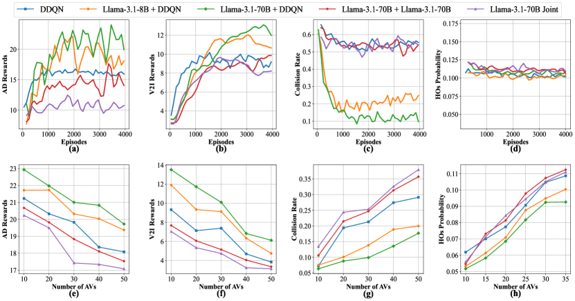
Figure 2: Simulation results and comparisons

III-C DDQN Based V2I Action Selection

As depicted in Fig. 1, LLMs will first make AD decisions ${a}^{\mathrm{AD}}_{j}$. Simultaneously, V2I observations ${n}_{R}^{j}$, ${n}_{T}^{j}$ are collected. The closest $M_{1}-1$ AVs with 3 features above are gathered to form a MDP. The DDQN processes this MDP to compute the V2I action ${a}^{\mathrm{V2I}}_{j}$. DDQN employs a neural network parameterized by $\boldsymbol{\theta}_{t}$ at each time step $t$ to approximate the $Q$-value function for a given state-action pair, i.e., $Q(\mathcal{S}^{\mathrm{V2I}}_{t},a^{\mathrm{AD}}_{t},a^{\mathrm{V2I}}_{t};\boldsymbol{\theta}_{t})$. To improve the stability and reliability of the estimates, DDQN uses a separate set of parameters, $\boldsymbol{\theta}_{t}^{\prime}$, for the target network, thereby decoupling the action selection from the value evaluation [6]. This decoupling mitigates the overestimation of $Q$-values that can occur in standard DQN. At each time step, the evaluation network with parameters $\boldsymbol{\theta}_{t}$ computes the $Q$-value, while the target network, parameterized by $\boldsymbol{\theta}_{t}^{\prime}$, provides stable $Q$-value estimates for the target. The evaluation network is trained by minimizing the mean squared error (MSE) loss $\mathcal{L}(\boldsymbol{\theta}_{t})$ between the predicted $Q$-values, $Q(\mathcal{S}^{\mathrm{V2I}}_{t},a^{\mathrm{AD}}_{t},a^{\mathrm{V2I}}_{t};\boldsymbol{\theta}_{t})$, and the target $Q$-values, $\hat{Q}(\mathcal{S}^{\mathrm{V2I}}_{t},a^{\mathrm{AD}}_{t},a^{\mathrm{V2I}}_{t};\boldsymbol{\theta}_{t}^{\prime})$, according to the Bellman equation as,

$$\mathcal{L}(\boldsymbol{\theta}_{t})=\mathbb{E}_{(s,a,r,s^{\prime})}\Bigg{[}\Big{(}r^{\mathrm{j,tele}}_{t}+\gamma Q\big{(} \mathcal{S}^{\mathrm{V2I}}_{t+1},$$ (10)

$$\arg\max_{{a^{\mathrm{V2I}}_{t+1}}^{\prime}}Q(\mathcal{S}^{\mathrm{V2I}}_{t+1},{{a^{\mathrm{V2I}}_{t+1}}^{\prime}};\boldsymbol{\theta}_{t});\boldsymbol{\theta}_{t}^{\prime}\big{)} -Q(\mathcal{S}^{\mathrm{V2I}}_{t},a^{\mathrm{AD}}_{t},a^{\mathrm{V2I}}_{t};\boldsymbol{\theta}_{t})\Big{)}^{2}\Bigg{]},$$

III-D Hybrid LLM-DDQN Learning and Convergence Analysis

As illustrated in Fig. 1, our proposed hybrid LLM-DDQN scheme consists of the following steps:
1) Collecting observations: The observation pool collects both V2I and AD data from the ego AV $j$ and the surrounding $M_{1}$ AVs. The observation will be separated into Transportation observations and V2I observations.
2) LLM-based AD decision-making: Using the transportation observations, relevant past examples are computed as described in Section III-B. This information is then incorporated into a task-oriented prompt, as outlined in Section III-A. The prompt is sent to the LLM, which returns an AD decision for the current time step.
3) DDQN-based V2I decision-making: Using the V2I observations from step 1 and the AD decision from step 2, the V2I action is determined via DDQN as in Section III-C.
4) Applying actions to target AVs: Both AD and V2I actions from steps 1 and 2, is applied to the target AV for implementation.
5) Storing examples in the example pool: After the AV executes its actions, if the AV terminates unexpectedly, the example is stored in the $\mathcal{E}^{\mathrm{bad}}$; otherwise, it is stored in the $\mathcal{E}^{\mathrm{good}}$ as explained in Section III-B.

Finally, we will analyze the convergence of the proposed hybrid LLM-DDQN scheme. It is worth noting that LLM-based AD decisions will serve as part of the V2I states as defined in Section II-C. It means that AD decisions can be considered as environment states for DDQN-based V2I systems. Therefore, for the AD side, LLM will produce a stable policy when enough examples are collected, which is similar to DDQN algorithms with experience pools. For the V2I side, since AD decisions can be considered as external states, the overall convergence will still hold.

IV Simulation and Performance Evaluation

We assume a total of 21 AVs traveling on a 3km single-direction, 4-lane highway. Along both sides of the highway, 5 RBSs and 20 TBSs are randomly positioned. This work includes two LLMs for AD decision-making:
1) Llama3.1-8B + DDQN: Llama3.1-8B is a small-scale model with 8 billion parameters, which is suitable for deployment at the network edge. 2) Llama3.1-70B + DDQN: Llama3.1-70B is the latest large-scale LLM model with 70 billion parameters, which has more powerful reasoning capabilities. 3) Llama3.1-70B + Llama3.1-70B: Employing two sequential Llama3.1 agents to perform AD and V2I actions simultaneously. 4) Llama3.1-70B Joint: Employing single Llama3.1 agents to generate Joint AD and V2I actions directly. We also include a DDQN baseline algorithm, which employs DDQN for joint optimization of V2I and AD [6]. The Markov decision process defined in Section II is shared across these benchmarks and our proposed solutions.

Fig. 2 presents the simulation results and comparisons. The performance metrics include the AD reward and V2I reward, as defined in (3) and (5), along with the collision rate and HO probability. In particular, Fig. 2(a) and (b) demonstrate that all LLM-based models show an improvement in both AD and V2I rewards, outperforming the DDQN baseline. Fig. 2(c) presents a reduction in collision rates as the number of episodes increases, with faster convergence being observed. These results highlight the ability of hybrid LLM models to balance experience replay and self-exploration, learning effectively from past examples and explorations to enhance their performance on target tasks. In addition, all algorithms have a similar HO probability.

Fig. 2(e) to (h) depict the performance variation as the number of AVs increases. Each data is captured by using the average performance of the last 200 episodes . As shown, increasing the number of AVs results in more congested highway scenarios, leading to more competitive resource allocation. This, in turn, results in higher HOs among the travelling vehicles. However, our proposed hybrid Llama+DDQN method still outperforms conventional DDQN approaches with higher average reward and lower collision rate. Finally, note that the LLM performance is closely related to its model size and designs. Specifically, Llama-3.1-70B outperforms Llama-3.1-8B because a larger model size usually indicates better reasoning and comprehension capabilities. Dual-agent or joint decision-making using LLMs does not perform well, as multi-task and multi-objective problems remain challenging for LLMs. These models struggle to learn effectively in complex scenarios with numerous constraints.

V Conclusion

LLMs have great potential for 6G networks, and this work proposed a hybrid LLM-DDQN scheme for joint V2I and AD optimization. It explores natural language-based optimization and network management, revealing the potential of LLM techniques. The simulations demonstrate that our proposed method can achieve faster convergence and higher learning efficiency than existing DDQN techniques.

References

- [1] H. Zhou, C. Hu, Y. Yuan, Y. Cui, Y. Jin, C. Chen, H. Wu, D. Yuan, L. Jiang, D. Wu et al., “Large language model (llm) for telecommunications: A comprehensive survey on principles, key techniques, and opportunities,” arXiv preprint arXiv:2405.10825, 2024.
- [2] Z. Yan and H. Tabassum, “Reinforcement learning for joint V2I network selection and autonomous driving policies,” in Proc. IEEE Glob. Commun. Conf., 2022, pp. 1241–1246.
- [3] I. T. U. (ITU), “Imt towards 2030 and beyond,” 2023. [Online]. Available: https://www.itu.int/en/ITU-R/study-groups/rsg5/rwp5d/imt-2030/Pages/default.aspx
- [4] L. Wen, D. Fu, X. Li, X. Cai, T. Ma, P. Cai, M. Dou, B. Shi, L. He, and Y. Qiao, “Dilu: A knowledge-driven approach to autonomous driving with large language models,” 2023.
- [5] D. Fu, X. Li, L. Wen, M. Dou, P. Cai, B. Shi, and Y. Qiao, “Drive like a human: Rethinking autonomous driving with large language models,” 2023.
- [6] Z. Yan and H. Tabassum, “Generalized multi-objective reinforcement learning with envelope updates in urllc-enabled vehicular networks,” arXiv preprint arXiv:2405.11331, 2024.
- [7] M. T. Hossan and H. Tabassum, “Mobility-aware performance in hybrid rf and terahertz wireless networks,” IEEE Transactions on Communications, vol. 70, no. 2, pp. 1376–1390, 2022.
- [8] H. Zhou, C. Hu, D. Yuan, Y. Yuan, D. Wu, X. Liu, Z. Han, and C. Zhang, “Generative ai as a service in 6g edge-cloud: Generation task offloading by in-context learning,” arXiv preprint arXiv:2408.02549, 2024.
- [9] Q. Dong, L. Li, D. Dai, C. Zheng, Z. Wu, B. Chang, X. Sun, J. Xu, and Z. Sui, “A survey on in-context learning,” arXiv preprint arXiv:2301.00234, 2022.