Calibrated Computation-Aware Gaussian Processes

Abstract

Gaussian processes are notorious for scaling cubically with the size of the training set, preventing application to very large regression problems. Computation-aware Gaussian processes (CAGPs) tackle this scaling issue by exploiting probabilistic linear solvers to reduce complexity, widening the posterior with additional computational uncertainty due to reduced computation. However, the most commonly used CAGP framework results in (sometimes dramatically) conservative uncertainty quantification, making the posterior unrealistic in practice. In this work, we prove that if the utilised probabilistic linear solver is calibrated, in a rigorous statistical sense, then so too is the induced CAGP. We thus propose a new CAGP framework, CAGP-GS, based on using Gauss-Seidel iterations for the underlying probabilistic linear solver. CAGP-GS performs favourably compared to existing approaches when the test set is low-dimensional and few iterations are performed. We test the calibratedness on a synthetic problem, and compare the performance to existing approaches on a large-scale global temperature regression problem.

1 Introduction

Gaussian processes are a powerful and flexible tool for Bayesian nonparametric regression, allowing a user to fit a wide array of possibly nonlinear phenomena using simple computational routines.

The most major challenge in scaling Gaussian processes to high-dimensional datasets is its cubic scaling with the number of training points, arising from the need to invert a Gramian matrix representing the prior covariance between data points (Rasmussen and Williams,, 2005). To address this, a wide array of computational approximations have been proposed, including iterative solvers (e.g. Wenger et al., 2022a ), approximations to the kernel matrix (e.g. Ferrari-Trecate et al., (1998)), and inducing point methods (e.g. Titsias, (2009)).

A particularly appealing approach recently proposed in Wenger et al., 2022b is CAGP. In this framework one uses a PLS to solve a linear system involving the Gramian matrix and then marginalises the uncertainty from the PLS. The result is an elegant cancellation that eliminates the need to invert the Gramian (see Section 2.2.2 for a more detailed explanation). The new posterior obtained is called “computation aware” because it is widened to represent additional computational uncertainty due to reduced computation in the PLS, compared to an exact (but computationally prohibitive) linear solve.

The most commonly used PLS for CAGP is an approach often called BayesCG (see Cockayne et al., 2019a )—in this setting called as CAGP-CG. This approach is favoured because of rapid mean convergence. One of the major challenges with CAGP-CG is that resulting CAGP is typically conservative—the posterior mean is much closer to the truth than the width of the posterior covariance suggests it should be. This is inherited from the widely observed poor calibration properties of BayesCG, which has been observed in several works including Cockayne et al., 2019a ; Bartels et al., (2019); Wenger and Hennig, (2020); Reid et al., (2023). We formally introduce calibration in Section 2.3. While some empirical Bayesian methods for mitigating this issue have been proposed (e.g., Wenger and Hennig, (2020); Reid et al., (2022, 2023)), they are difficult to apply within CAGP as the choice of prior is heavily constrained by the method.

1.1 Contributions

The contributions of this paper are as follows:

• We rigorously prove that, if a calibrated PLS is used, the resulting CAGP is calibrated (Theorem 4).

• We introduce a new class of CAGP based on PSIM (as seen in Cockayne et al., (2021)).

• We explore efficient implementation of a new CAGP approach based on Gauss-Seidel iterations (CAGP-GS, Section 4.2). CAGP-GS scales favourably compared to CAGP-CG in regimes where only a small number of test points are required.

• We explore the empirical properties of CAGP-GS on a synthetic test problem and a large-scale geospatial regression problem (Sections 5.1 and 5.2). In particular, we note that for small iteration numbers, CAGP-GS outperforms all known alternative CAGP frameworks in terms of mean convergence and uncertainty quantification.

1.2 Structure of the Paper

The rest of the paper proceeds as follows. In Section 2 we discuss the required background on CAGP, PLS and calibratedness. Section 3 discusses calibratedness in the context of CAGP, while Section 4 presents a particular class of PLS that are both calibrated and can be used in the CAGP framework. Section 5 presents simulations demonstrating the new methodology, and we conclude in Section 6. Proofs and additional results for experiments from Section 5 are included in the supplementary material.

2 Background

2.1 GP Regression

Suppose $f\sim\mu_{0}=\mathcal{GP}(m_{0},k)$, where $k$ is a positive definite kernel function. Consider GP inference under the observation model

$$y=f(X)+\zeta$$ (1)

where $X\subset D$ is a set of $d$ distinct training points the domain of $f$, while $\zeta\sim\mathcal{N}(0,\sigma^{2}I)$. It may be helpful to think of $D$ as a subset of $\mathbb{R}^{n}$ for some $n$, but this is not required. The predictive distribution conditional on this information at a set of $d_{\textsc{test}}$ test points $X^{\prime}$ is given by

$$f(X^{\prime})\mid y \sim\mu=\mathcal{GP}(\bar{m},\bar{k})$$ (2a)

$$\bar{m}(X^{\prime}) =m_{0}(X^{\prime})+k(X^{\prime},X)v^{\star}$$ (2b)

$$\bar{k}(X^{\prime},X^{\prime}) =k(X^{\prime},X^{\prime})-k(X^{\prime},X)G^{-1}k(X,X^{\prime})$$ (2c)

where $G=K(X,X)+\sigma^{2}I$, while $v^{\star}$ is the solution to the linear system

$$Gv^{\star}=b.$$ (3)

with $b=(y-m_{0}(X))$.

As has been widely noted (e.g., in Rasmussen and Williams, (2005)), one of the major challenges of the GP regression is that the complexity of the computations above is $\mathcal{O}(d^{3})$ owing to the inversion of the Gramian matrix $G$. Recent work (Wenger et al., 2022b ) proposes a novel framework to mitigate this cost called CAGP, introduced next.

2.2 Computation-Aware GPs

CAGP center on use of PLS to solve the system Eq. 3. We will first outline the literature on the PLS before discussing CAGP themselves in Section 2.2.2.

2.2.1 (Bayesian) PLS

At the most generic level, PLS are PNM (Hennig et al., (2022); Cockayne et al., 2019b ) for solving linear systems, that is, they are learning procedures that return a probability distribution intended to quantify error due to having expended reduced computational effort to calculate $v^{\star}$. It is common for such learning procedures to depend on some “prior” belief about $v^{\star}$, expressed through the distribution $\eta_{0}$. So we use the notation $\eta:\mathcal{P}(\mathbb{R}^{d})\times\mathbb{R}^{d}\to\mathcal{P}(\mathbb{R}^{d})$ or $(\eta_{0},b)\mapsto\eta(\eta_{0},b)$, where $\mathcal{P}(\mathbb{R}^{d})$ is the set of all probability measures on $\mathbb{R}^{d}$ for a PLS. We will limit attention to Gaussian learning procedures, i.e. those that accept Gaussian input $\eta_{0}=\mathcal{N}(m_{0},C_{0})$ and return a Gaussian output $\eta(\eta_{0},b)=\mathcal{N}(\bar{v},\bar{C})$. The particular prior $\eta_{0}=\mathcal{N}(0,G^{-1})$ (referred to as the “inverse prior” in this paper) is intrinsic to CAGP, and we will limit attention to this throughout the following sections. However, note that material in Sections 2.2.1 and 2.4 can be generalised to arbitrary priors.

Many PLS have a Bayesian interpretation, i.e. they are based on conditioning $\eta_{0}$ on observations of the form $z_{m}=S_{m}^{\top}b$, where $S_{m}\in\mathbb{R}^{d\times m}$ is a matrix of search directions with linearly independent columns. Under such observations and the inverse prior, the posterior is

$$v\mid z_{m}=\eta \sim\mathcal{N}(\bar{v}_{m},\bar{C}_{m})$$ (4a)

$$\bar{v}_{m} =S_{m}(S_{m}^{\top}GS_{m})^{-1}S_{m}^{\top}b$$ (4b)

$$\bar{C}_{m} =G^{-1}-D_{m}^{\textsc{Bayes}}$$ (4c)

$$\bar{D}_{m}^{\textsc{Bayes}} =S_{m}(S_{m}^{\top}GS_{m})^{-1}S_{m}^{\top}.$$ (4d)

This posterior is not directly computable, as computing $\bar{C}_{m}$ requires computation of $G^{-1}$, which we assumed in Section 2.1 we did not want to compute. Nevertheless, as we will see in Section 2.2.2, this choice leads to some cancellations for CAGP.

Choice of Search Directions

Generic choices of $S_{m}$ that have been examined in the literature include standard Euclidean basis vectors and random unit vectors (Cockayne et al., 2019a, ; Wenger et al., 2022b, ; Pförtner et al.,, 2024). However, these typically suffer from slow convergence of $v_{m}\to v^{\star}$ compared to state-of-the-art iterative methods, making them unattractive.

A particularly important choice of $S_{m}$ are those based on CG. In this case the PLS is often referred to as BayesCG (Cockayne et al., 2019a, ). These directions are favoured because (i) they can be proven to converge at an exponential rate in $m$ in the worst case (often faster in practice), and (ii) they are $G$-conjugate, meaning that $S_{m}^{\top}GS_{m}$ is diagonal. As a result the posterior reported in Eq. 4 simplifies further. On the other hand, these directions result in poor calibration of the posterior, which will be discussed further in Section 2.3.

Computational Complexity

Ignoring the cost of computing $G^{-1}$, the complexity of computing Eqs. 4b and 4d is $\mathcal{O}(m(m^{2}+d^{2}))$ owing to the inversion of the $m\times m$ matrix $S_{m}^{\top}GS_{m}$ and the requirement to compute (dense) products of the form $GS_{m}$ which have complexity $\mathcal{\mathcal{O}}(md^{2})$. Thus, if $m\ll d$ the complexity compared to a direct method is significantly reduced. For BayesCG the diagonal matrix inversion is reduced to $\mathcal{O}(m)$, so that the complexity is only $\mathcal{O}(md^{2})$.

2.2.2 The Marginalisation Trick

The central “trick” behind CAGP is that, given any belief from a PLS of the form

$$v\sim\eta=\mathcal{N}(\bar{v},G^{-1}-D)$$ (5)

we can construct a new belief over $f(X^{\prime})$ through the marginalisation

$$\tilde{p}(f)=\int_{\mathbb{R}^{d}}p(f(X^{\prime})\mid v)\eta(\mathrm{d}v)$$ (6)

the law of which we denote $\tilde{\mu}$. Since all the involved distributions are Gaussian, Wenger et al., 2022b derived the modified posterior as

$$\tilde{\mu} =\mathcal{GP}(\tilde{m},\tilde{k})$$ (7)

$$\tilde{m}(X^{\prime}) =m_{0}(X^{\prime})+k(X^{\prime},X)\bar{v}$$ (8)

$$\tilde{k}(X^{\prime},X^{\prime}) =k(X^{\prime},X^{\prime})-k(X^{\prime},X)Dk(X,X^{\prime}).$$ (9)

Notably, the presence of $G^{-1}$ in $\eta$ is crucial as it leads to cancellation of the downdate involving $G^{-1}$ from Eq. 2c. As a result we need only calculate the $D$ term in the underlying PLS, negating any need to invert $G$. If $D$ can be computed at significantly lower complexity than $G^{-1}$, as in Section 2.2.1, then the overall cost of GP inference is reduced. Moreover, Wenger et al., 2022b (, Section 2) demonstrates that $\tilde{k}(X^{\prime},X^{\prime})$ is “wider” than $\bar{k}(X^{\prime},X^{\prime})$ and can be interpreted as providing additional uncertainty quantification for the reduced computation.

Algorithm 1 Computation Aware GP

cagp$X$, $y$, $X^{\prime}$, $\sigma^{2}$

1:$b=y-m_{0}(X)$

2:$V=k(X^{\prime},X)$

3:$G(v)=v\mapsto k(X,X)v+\sigma^{2}v$

4:$\tilde{v},\tilde{D}=\textsc{cagp\_pls}(G,b,V)$

5:$\tilde{m}=m_{0}(X^{\prime})+\tilde{v}$

6:$\tilde{k}=k(X^{\prime},X^{\prime})-\tilde{D}$

7:$\tilde{m},\tilde{k}$

Algorithm 1 gives an implementation of this as pseudocode. Note that it is assumed cagp_pls requires access to $G$ only through its action on vectors $v$, rather than explicitly, allowing for a matrix-free implementation. Algorithm 1 is a slightly modified version of that presented in Wenger et al., 2022b ; the quantities $\tilde{v}$ and $\tilde{D}$ returned by the routine cagp_pls are given by $\tilde{v}=V\bar{v}=k(X^{\prime},X)\bar{v}$, and $\tilde{D}=VDV^{\top}=k(X^{\prime},X)Dk(X,X^{\prime})$, i.e. they are the image of $\eta$ under the map $v\mapsto Vv$. This is more commensurate with the novel algorithms we will introduce in Sections 3 and 4.

Going forward we will use CAGP-CG to refer to a CAGP using BayesCG as the PLS.

2.3 Calibrated Learning Procedures

While BayesCG has several numerically appealing properties, as already mentioned it is poorly calibrated. In particular the uncertainty quantification provided is conservative, meaning that the posterior covariance $\bar{C}_{m}$ is typically much wider than the error $\bar{v}_{m}-v^{\star}$.

This is due to an incorrect application of Bayesian inference in constructing the posterior. It can be shown (Golub and Van Loan,, 2013, Section 11.3.3) that (when the initial guess for the solution is zero) the CG directions form a basis of the Krylov subspace

$$K_{m}(G,b) =\textup{span}(b,Gb,G^{2}b,\dots,G^{m-1}b)$$

$$=\textup{span}(Gv^{\star},G^{2}v^{\star},\dots,G^{m}v^{\star}).$$

If we ignore the orthogonalisation of the search directions (which would not affect the posterior in a Bayesian inference problem) this results in information of the form $z_{i}=s_{i}^{\top}Gv^{\star}=(v^{\star})^{\top}G^{i+1}v^{\star}$, $i=1,\dots,m$, each of which is quadratic in $v^{\star}$ rather than linear. Linearity of the information $z_{i}$ is intrinsic to the Gaussian conditioning argument that underpins PLS, and ignoring this yields the poor calibration of BayesCG-based PLS.

In this paper we will discuss how another class of PLS can be used in the CAGP framework. These PLS do not have a Bayesian interpretation, but can nevertheless be said to be calibrated in a formal sense. We will be interested in the question of whether, when the PLS is calibrated, the derived CAGP is also calibrated, so we present this rather generically. Cockayne et al., (2022) introduces the notion of strong calibration, a more intuitive description of which is given below; we refer the reader to the aforementioned paper for a formal introduction.

Briefly, a learning procedure $\mu:\mathcal{P}(\mathcal{U})\times\mathcal{Y}\to\mathcal{P}(\mathcal{U})$ is said to be strongly calibrated with respect to a distribution $\mu_{0}$ and a data-generating model $\textsc{dgm}:\mathcal{U}\to\mathcal{Y}$ if, under the following procedure:

1. $u^{\star}\sim\mu_{0}$

2. $y=\textsc{dgm}(u^{\star})$

it holds that, on average over $\mu_{0}$, $u^{\star}$ is a “plausible sample” from the posterior $\mu(\mu_{0},y)$. The last statement can be made formal in several ways, but a particularly simple definition for the case of Gaussian learning procedures is given by Cockayne et al., (2021).

Definition 1 (Cockayne et al., (2021, Definition 6 and 9)).

Consider a fixed Gaussian prior $\mu_{0}=\mathcal{N}(u_{0},\Sigma_{0})$, a data-generating model dgm and a learning procedure $\mu(\mu_{0},y)=\mathcal{N}(\bar{u},\bar{\Sigma})$. Suppose that $\bar{\Sigma}$ is independent of $y$ and potentially singular, with $N$ and $R$ matrices whose columns form (mutually) orthonormal bases of its null and row spaces respectively. Then $\mu$ is said to be strongly calibrated to $(\mu_{0},\textup{{dgm}})$ if:

1. $(R^{\top}\bar{\Sigma}R)^{-\frac{1}{2}}R^{\top}(\bar{u}-u^{\star})\sim\mathcal{N}(0,I)$.

2. $N^{\top}(\bar{u}-u^{\star})=0$

when $u^{\star}\sim\mu_{0}$.

Note that in Definition 1 the randomisation of $u^{\star}$ induces randomness in $\bar{u}$ through dependence on $y$, making the statement rather nontrivial. The assumption that $\bar{\Sigma}$ is independent of $y$ is important to ensure that the range and null spaces are consistent across draws from $\mu_{0}$; this can be relaxed, but resulting definitions are far less analytically tractable. Lastly in the case that $\bar{\Sigma}$ is full rank, the second of the two conditions is redundant.

Definition 1 provides a theoretical framework for validating strong calibration, but we are also interested in validating this numerically. To accomplish this, we will apply the simulation-based calibration tests of Talts et al., (2018); these are described in more detail in Appendix B.

2.4 Probabilistic Stationary Iterative Methods

Another subclass of PLS are PSIM, introduced in Cockayne et al., (2021). PSIM are based on an underlying stationary iterative method for solving the linear system (see e.g. Young, (1971)), that is, methods that evolve an iterate $v_{m}$ according to the map $v_{m}=P(v_{m-1})$, with some user-supplied initial guess $v_{0}$. Given such a method, the associated PSIM is obtained by pushing the prior $\eta_{0}$ through the map $P^{m}$ defined by composing $P$ with itself $m$ times. We will restrict attention to affine $P$, i.e. $P(v)=Mv+g$, where $M\in\mathbb{R}^{d\times d}$ while $g\in\mathbb{R}^{d}$. Then, for Gaussian $\eta_{0}=\mathcal{N}(0,G^{-1})$ the output of the PSIM is given by

$$\eta_{m} =\mathcal{N}(v_{m},C_{m})$$ (10a)

$$v_{m} =P^{m}(0)=\sum_{i=0}^{m-1}M^{i}g$$ (10b)

$$C_{m} =M^{m}G^{-1}(M^{\top})^{m}$$ (10c)

Since the output of a PSIM is not a Bayesian posterior, several important questions arise: (i) when does the posterior contract around the truth, and (ii) is the output calibrated in the sense of Definition 1. For (i), Cockayne et al., (2021, Proposition 2) establishes that provided the underlying stationary iterative method converges to the true solution, the PSIM contracts around the true solution, and does so at the same rate as the error converges in any norm on $\mathbb{R}^{d}$. For (ii), Cockayne et al., (2021, Propositions 7 and 10) show that any PSIM based on appropriate affine $P$ is strongly calibrated in the sense of Definition 1, provided $M$ is diagonalisable (over $\mathbb{C}$). This is a fairly mild restriction considering the density of diagonalisable matrices (Gorodentsev,, 2017, Chapter 2).

In the next sections we will demonstrate how PSIM can be adapted to work with CAGP, and discuss transfer of calibratedness in this setting.

3 Calibrated Computation-Aware GPs

In this section we prove that CAGP are calibrated if a calibrated PLS is used to solve Eq. 3. First we observe that the reparameterisation in Eq. 2 can be formulated as Bayesian inference with an alternative observation model.

Proposition 2.

It holds that $f\mid y$ from Eq. 2 is equal to the posterior $f\mid v$ from Bayesian inference under the observation model:

$$v\mid f=G^{-1}b=G^{-1}(f(X)-m_{0}(X))+\bar{\zeta}$$

where $\bar{\zeta}\sim\mathcal{N}(0,\sigma^{2}G^{-2})$.

The next corollary establishes that under the observation model used in Proposition 2, the prior distribution adopted in CAGP is correct in a subjective Bayesian sense.

Corollary 3.

The a-priori marginal distribution of $v$ is $v\sim\mathcal{N}(0,G^{-1})$.

This is an important result for calibration, since to be able to talk about calibrated posteriors for Eq. 3 we first need to know that if the prior on $f$ is correct, the prior on $v$ is also correct.

The next result is the central result of the paper, establishing calibratedness of CAGP when a calibrated PLS is used.

Theorem 4.

Suppose that $f\sim\mathcal{GP}(m_{0},k)$ and $y\mid f=f(X)+\zeta$, where $k$ is a positive definite kernel. Further, suppose that the PLS in Eq. 5 is a learning procedure that is calibrated for $\mathcal{N}(0,G^{-1})$, and satisfies the following conditions:

1. $D$ is independent of $y$.

2. $\textup{Cov}(f(X^{\prime}),\bar{v})=K(X^{\prime},X)G^{-1}\textup{Cov}(y,\bar{v})$.

Then the CAGP posterior is calibrated for the original GP prior and the original data generating model.

Regarding the conditions above, as mentioned previously, Condition 1 is satisfied by most PLS, with the notable exception of those where some calibration procedure has been applied to choose the prior. Condition 2 seems technical, but is in fact satisfied under mild conditions.

Corollary 5.

Suppose that the assumptions of Theorem 4 are satisfied, and further that $\bar{v}$ is an affine map of $y$, i.e. $\bar{v}=My+g$. Then the CAGP posterior is calibrated for the original GP prior and original data generating model.

Note that the requirements of Corollary 5 are satisfied by any Bayesian procedure, as well as for the probabilistic iterative methods we will introduce in the next section. An important exception is CAGP-CG since, as mentioned in Section 2.2.1, in this case the map is not affine owing to dependence of $S_{m}$ on $v^{\star}$. Having established this result, we next proceed to show how PSIM can be integrated with CAGP to provide calibrated uncertainty.

4 Probabilistic Stationary Iterative Methods with the Inverse Prior

To embed a probabilistic stationary iterative method in a CAGP we need to obtain an output measure as in Eq. 5. We now show that for all reasonable PSIM, $C_{m}$ from Eq. 10c can be rearranged to have this structure.

4.1 Convergent Linear Stationary Iterative Methods

As mentioned in Section 2.4, convergence of stationary iterative methods is not guaranteed for all affine maps $P$. We therefore limit attention to completely consistent methods (Young,, 1971, Section 3.2 and 3.5). These methods have the property that, if they converge, they are guaranteed to converge to the true solution, and therefore they are the widest class of reasonable stationary iterative methods to use for solving a linear system.

For nonsingular $G$, any completely consistent iterative method can be written in the form $M=I-\tilde{M}G,\;g=\tilde{M}b$ where $\tilde{M}$ is a nonsingular matrix. The next proposition shows that the iterations of any PSIM based on a completely consistent iterative method can be written in a form commensurate with CAGP.

Proposition 6.

Let $\eta_{m}$ be the $m$^th iterate of a probabilistic iterative method whose underlying stationary iterative method is completely consistent. Then $\eta_{m}\sim\mathcal{N}(\bar{v}_{m},G^{-1}-D_{m})$, where $\bar{v}_{m}$ is the $m$^th iterate of the stationary iterative method with $v_{0}=0$, while $D_{0}=0$ and

$$D_{m}=\tilde{M}+\tilde{M}^{\top}-\tilde{M}G\tilde{M}^{\top}+(I-\tilde{M}G)D_{m-1}(I-\tilde{M}G)^{\top}.$$ (11)

While it is useful to know that this holds for any completely consistent probabilistic iterative method, it is not clear that the above computations can be made to be efficient. Moreover, we still need to ensure that the iterative method converges, as it will be highly problematic for embedding within GP regression otherwise. In the next section we consider a particular instance of a probabilistic iterative method which is provably convergent for any symmetric positive definite matrix.

4.2 Gauss-Seidel

The Gauss-Seidel method partitions $G=L+U$, where $L$ is the lower-triangular part of $G$ and $U$ is the strict upper triangular part. We then take $M=-L^{-1}U$ and $g=L^{-1}b$. Golub and Van Loan, (2013, Theorem 11.2.3) establishes that Gauss-Seidel converges to the true solution for any initial guess $v_{0}$ provided $G$ is symmetric positive-definite, making it particularly attractive for CAGP.

To apply Proposition 6 we must first identify $\tilde{M}$. Note that $U=G-L$, so that $M=-L^{-1}U=I-L^{-1}G$; thus $\tilde{M}=L^{-1}$. Also note that if $D_{G}$ is the diagonal of $G$, since $G$ is symmetric positive definite, we have that $U=(L-D_{G})^{\top}$. The $D_{i}$ from Proposition 6 can then be simplified:

$$L^{-1}GL^{-\top} =L^{-1}(L+L^{\top}-D_{G})L^{-\top}$$

$$=L^{-1}+L^{-\top}-L^{-1}D_{G}L^{-\top}$$

so that $D_{1}=L^{-1}D_{G}L^{-\top}$, and

$$D_{i} =L^{-1}D_{G}L^{-\top}+MD_{i-1}M^{\top}$$

$$=L^{-1}D_{G}L^{-\top}+L^{-1}UD_{i-1}U^{\top}L^{-\top}.$$

We therefore have the following non-recursive expression for the downdate:

$$D_{m}=\sum_{i=0}^{m-1}(L^{-1}U)^{i}L^{-1}D_{G}L^{-\top}(U^{\top}L^{-\top})^{i}.$$ (12)

We can also establish several important properties of this PLS, in the following proposition:

Proposition 7.

The covariance matrix $G^{-1}-D_{m}$ from probabilistic Gauss-Seidel has rank $d-1$ for all $m\geq 1$, and its null space is equal to $\textup{span}(L^{\top}e_{d})$, where $e_{d}$ is the $d$^th Euclidean basis vector.

Considering Section 2 we can therefore implement cagp_pls with Gauss-Seidel as described in Algorithm 2.

Algorithm 2 CAGP-GS

cagp_pls_gs$G$, $b$, $V$, $m$

1:$Z_{1}=L^{-\top}V^{\top}$

2:$z=L^{-1}b$

3:$v_{1}=z$

4:$\tilde{Z}_{1}=D_{G}^{\frac{1}{2}}Z_{1}$ $i=2$ to $m$

5:$v_{i}=z-L^{-1}Uv_{i-1}$

6:$Z_{i}=L^{-\top}U^{\top}Z_{i-1}$

7:$\tilde{Z}_{i}=D_{G}^{\frac{1}{2}}Z_{i}$

8:$\tilde{v}=Vv_{i}$, $\tilde{D}=\sum_{i=1}^{m}\tilde{Z}_{i}^{\top}\tilde{Z}_{i}$

4.2.1 Complexity

Since $L^{-1}$ is lower triangular, the action of $L^{-1}$ and $L^{-\top}$ can be computed using forward and back substitution, having complexity $\mathcal{O}(d^{2})$ The computational complexity of Algorithm 2 is thus $\mathcal{O}(mdd_{\textsc{test}}(d+d_{\textsc{test}}))$.

As mentioned in Section 2.2.1, the cost of CAGP-CG is $\mathcal{O}(md^{2})$ to compute the posterior over $v$. Once this has been computed, computing the implied $\tilde{v}$ and $\tilde{D}$ costs, respectively $\mathcal{O}(dd_{\textsc{test}})$ and $\mathcal{O}(md_{\textsc{test}}(d+d_{\textsc{test}}))$, for an overall complexity of $\mathcal{O}(m(d^{2}+dd_{\textsc{test}}+d_{\textsc{test}}^{2}))$.

In terms of memory, for CAGP-GS we need to store the matrix $Z_{i}$ for complexity $\mathcal{O}(dd_{\textsc{test}})$; computed factors can be saved to disk and loaded later to compute $\tilde{D}$ (which is only $d_{\textsc{test}}\times d_{\textsc{test}}$). For CAGP-CG only $\mathcal{O}(d)$ memory is required at execution time. This ignores storage of $G$ (required for both algorithms); however since each algorithm requires only the action of $G$ (or $L$, $U$) on matrices / vectors, a matrix-free implementation is possible (though this is not explored in this paper). Also note that this highlights that to apply CAGP-CG on a new set of test points does not require rerunning the algorithm, while for CAGP-GS we need to do so.

Clearly CAGP-GS has a higher complexity than CAGP-CG, though under the assumption that $d\gg m,d_{\textsc{test}}$ the leading order of both algorithms is $\mathcal{O}(d^{2})$, so in this setting the costs should still be comparable. In the next section we will consider the empirical performance of CAGP-GS compared to CAGP-CG.

5 Experiments

5.1 Synthetic Problem

We first consider a synthetic test problem, so that we can test for calibratedness. We take $m_{0}=0$ and $k$ to be a Matèrn $\nicefrac{{3}}{{2}}$ covariance with amplitude set to $1$, and will vary the length-scale. For the data-generating model we set $\sigma=0.1$. We set our domain to be $D=[0,1]^{2}$ and generate our training points by sampling $400$ points uniformly at random. Test points are a regular grid with spacing $0.05$, i.e. generating $21\times 21$ equally spaced points for a total of $d=441$ points. The underlying true function is taken to be sample from the prior, so that the calibration guarantee from Corollary 5 can be tested.

Plots of convergence for the posterior mean as a function of $m$, with length scales set to $0.1,0.2$ and $0.4$, averaged over 50 runs, can be seen in Fig. 1. We compare CAGP-GS to both CAGP-CG and CAGP-Rand, a method that uses a Bayesian PLS with $S_{i}$ having IID normal entries. This approach should be calibrated, but shows slow convergence typical of most Bayesian PLS not using CG directions. Unexpectedly, the posterior mean for CAGP-GS initially converges faster than that from CAGP-CG for all length-scales, though ultimately it is overtaken by CG. However, in expensive problems where few iterations can be performed, this suggests that CAGP-GS should be preferred to CAGP-CG owing to its initially faster convergence with calibration guarantees. As a function of the length-scale, it appears that this behaviour is less pronounced for smaller values, in which cases the matrix will typically be better conditioned.

Figure 1: Mean Convergence for the synthetic problem in Section 5.1.

In Fig. 2 we highlight the uncertainty quantification properties of CAGP-GS compared to CAGP-CG and CAGP-Rand using the simulation-based calibration method described in Algorithm 3 for $N_{\textsc{sim}}=1000$ simulations, with length-scale now fixed to $\ell=0.2$ and $m=5$ iterations. We also report the result of a Kolmogorov-Smirnov test for uniformity. As implied by Theorem 4, both CAGP-GS and CAGP-Rand are calibrated (p-values 0.6689 and 0.6802), while CAGP-CG shows the expected inverted U-shape characteristic of an overly conservative posterior and has a $p$-value of 0.0084.

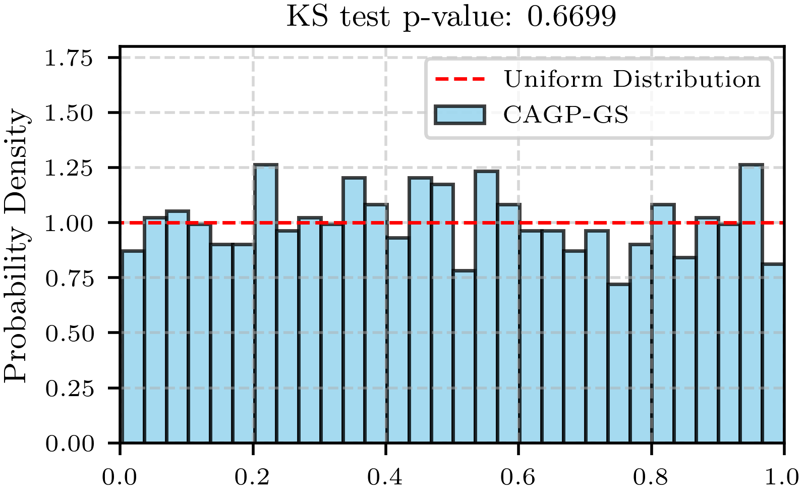
(a) CAGP-GS

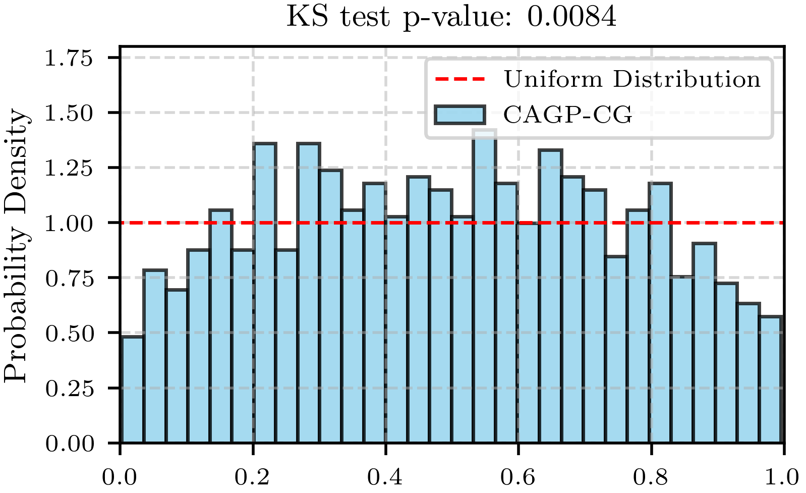
(b) CAGP-CG

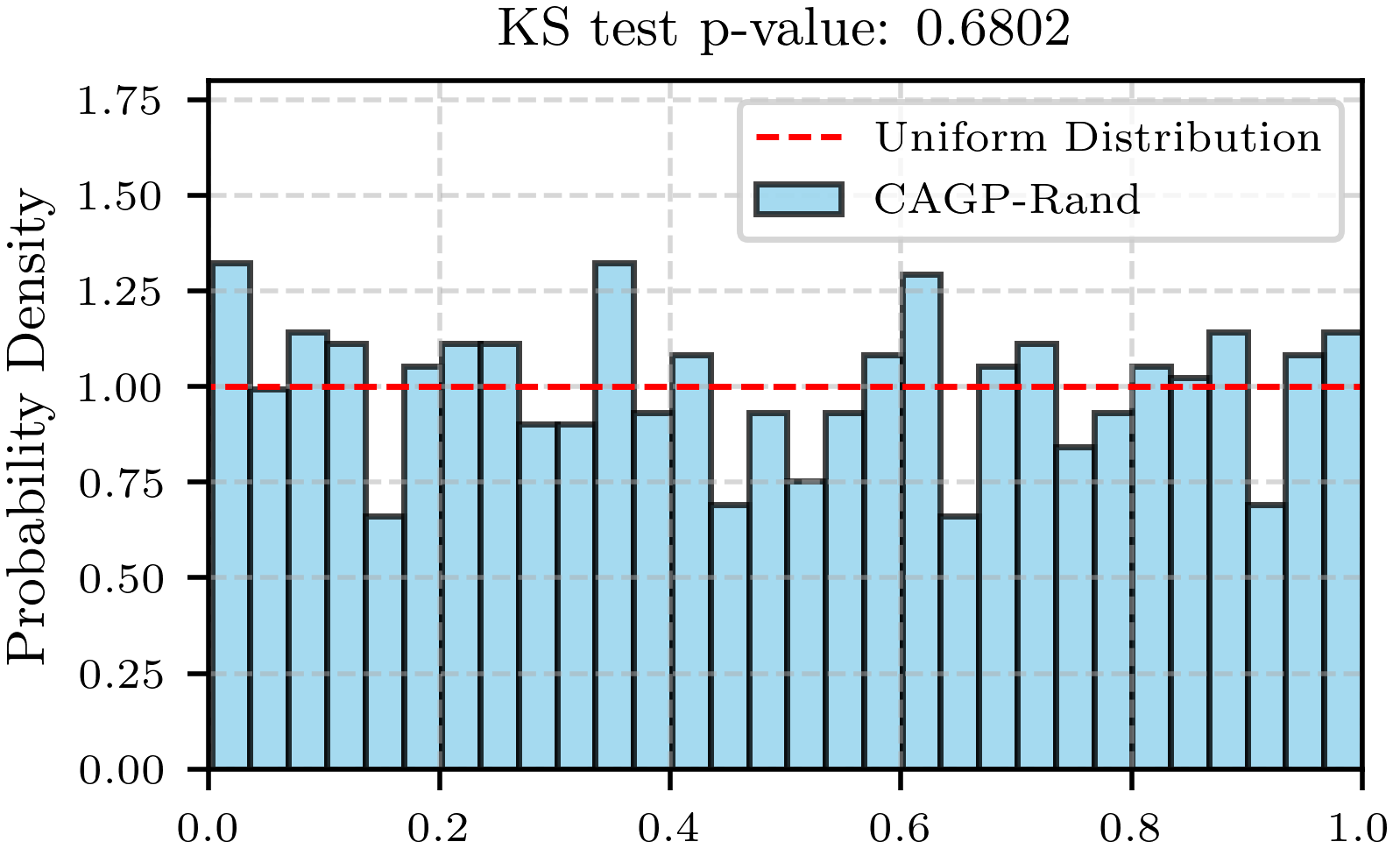
(c) CAGP-Rand

Figure 2: Simulation-based calibration results for the synthetic problem described in Section 5.1.

5.2 ERA5 Regression

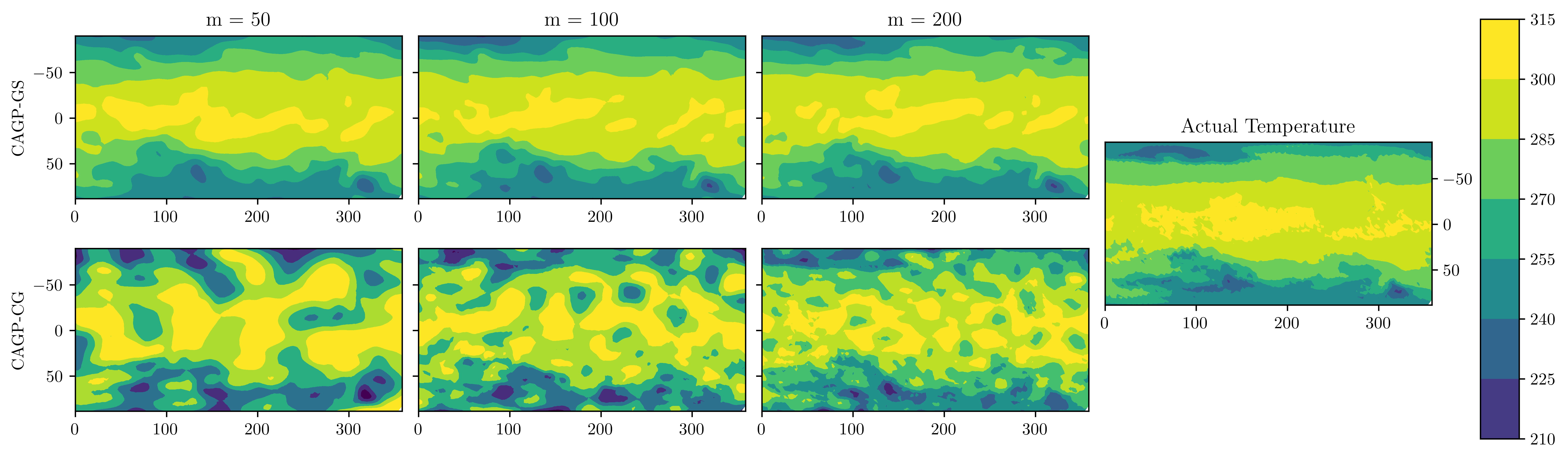
Figure 3: Sequences of posterior means for the large-scale regression from Section 5.2, as a function of $m$. The x and y axes represent longitudes and latitudes respectively, and the contours indicate the temperature in Kelvin.

In this section we run a geospatial regression problem on the ERA5 global 2 metre temperature dataset (Hersbach et al.,, 2023). This is a reanalysis dataset with approximately 31 km resolution, and has temporal coverage from 1940 to present. For the purposes of this demonstration we limit our attention to a single timestamp on 1st January 2024 at 00.00. This results in a grid of a total of $\approx 1$ million points. To obtain matrices that can be more easily represented in memory these points were downsampled as described in the results below.

To fix a prior we used a Matèrn $\nicefrac{{3}}{{2}}$ covariance function, and optimised hyper-parameters by maximising marginal likelihood (see Rasmussen and Williams, (2005, Sec. 2.2)) on a coarse uniform grid of $72\times 144$ points on the globe. We use a constant prior mean fixed to the average of the data points.

We first examine qualitative convergence of the method by presenting plots of the posterior mean obtained from CAGP-GS and CAGP-CG for a uniformly spaced grid of $28,000$ training and $7,225$ test points in Fig. 3. Interestingly the CAGP-GS posterior means are considerably smoother than the CAGP-CG posterior means; this smoother convergence may be more desirable in low iteration number regimes, and is likely due to known smoothing properties of Gauss-Seidel (see e.g. Xu and Zikatanov, (2017, Section 5.5)).

In Fig. 4, we compare the wall-time taken to compute the posterior mean and covariance using CAGP-GS and CAGP-CG. In each plot we vary one parameter, fixing the others to $m=80,d=10638,d_{\textsc{test}}=25$. Results were computed on a high-performance computing service on a single node with 40 cores. The results are mostly as expected from Section 4.2.1. With increasing iterations, CAGP-GS and CAGP-CG scale similarly, with CAGP-GS performing slightly better for higher iterations. With increasing $d$ CAGP-CG is initially faster, but CAGP-GS takes over in the later part. For small $d_{\textsc{test}}$ CAGP-GS performs better, but CAGP-CG improves as $d_{\textsc{test}}$ increases and becomes comparable to $d$.

Finally, we test the calibratedness for a uniformly spaced grid of $d=64,700$ training points and $d_{\textsc{test}}=100$ held out test points. Note that in this setting Theorem 4 does not provide a calibration guarantee, and in particular our theory says nothing about calibratedness on held-out data. Nevertheless, it is interesting to see whether some version of calibratedness is obtained in a practical setting. For this $d$, $G$ requires around 30 GB of storage, so is around the largest that can practically be considered without matrix-free implementations. Histograms of $t_{i}=\Phi\left(\frac{\tilde{m}(x_{i})-f(x_{i})}{sd(x_{i})}\right)$ for test points $x_{i}$ are shown in Fig. 5. The Kolmogorov-Smirnov test for uniformity gives a p-value of $0.4707$ for CAGP-GS and $5.0112\times 10^{-1}$ CAGP-CG. This shows that CAGP-GS is closer to calibrated, and CAGP-CG remains miscalibrated.

6 Conclusion

The theoretical and computational results presented above provide a clear motivation for considering PLS other than BayesCG for CAGP. Mean convergence is faster for small $m$ as shown in Fig. 1, and the posterior mean plots in Fig. 3 show recoveries that, we would argue, retain more of the smoothness and structure of the prior than those for CAGP-CG. Further, with an appropriate GP calibration approach it appears we can obtain reasonably well-calibrated CAGP even outside of the synthetic calibration guarantees of Theorem 4.

The principle downsides of CAGP-GS are (i) higher computational complexity and (ii) worse scaling for large $m$. On (i) we would argue that this approach should only be used in a small $d_{\textsc{test}}$ regime which, in very large scale regression problems, is likely to be a limitation in any case. For (ii) we would argue that small $m$ is the regime in which well-calibrated CAGP are most attractive, since for larger $m$ the added computational uncertainty is dominated by the mathematical uncertainty. Moreover, we feel that the calibration benefits are enough to justify these disadvantages.

There are several interesting future research directions. First, we have not explored matrix-free methods to scale to “big data” problems. Efficient, parallelisable matrix-free implementations of $L^{-\top}$ are challenging due to the inherently sequential nature of backward substitution, but would nevertheless allow further scaling. Second, we would like to explore further accelerations of calibrated CAGP. One avenue that seems promising is to combine CAGP-GS and CAGP-CG; this would sacrifice calibratedness but, if GS is either used in the initial convergence period or interleved with CG iterations to provide smoothing, this may result in superior mean convergence.

Appendix A Proofs of Theoretical Results

Proof of Proposition 2.

This is demonstrated by direct calculation. We have that $f(X^{\prime})$ and $v$ are jointly Gaussian:

$$\begin{bmatrix}f(X^{\prime})\\ v\end{bmatrix} \sim\mathcal{N}\left(\begin{bmatrix}m_{0}(X^{\prime})\\ 0\end{bmatrix},\begin{bmatrix}k(X^{\prime},X^{\prime})&k(X^{\prime},X)G^{-1}\\ G^{-1}k(X,X^{\prime})&G^{-1}k(X,X)G^{-1}+\sigma^{2}G^{-2}\end{bmatrix}\right).$$

Clearly

$$G^{-1}k(X,X)G^{-1}+\sigma^{2}G^{-2} =G^{-1}(k(X,X)+\sigma^{2}I)G^{-1}$$

$$=G^{-1}$$

and so

$$\begin{bmatrix}f(X^{\prime})\\ v\end{bmatrix} \sim\mathcal{N}\left(\begin{bmatrix}m_{0}(X^{\prime})\\ 0\end{bmatrix},\begin{bmatrix}k(X^{\prime},X^{\prime})&k(X^{\prime},X)G^{-1}\\ G^{-1}k(X,X^{\prime})&G^{-1}\end{bmatrix}\right).$$

Applying the Gaussian conditioning formula we obtain

$$\mathbb{E}[f(X^{\prime})\mid v] =m_{0}(X^{\prime})+k(X^{\prime},X)G^{-1}Gv$$

$$=m_{0}(X^{\prime})+k(X^{\prime},X)v$$

$$\mathbb{V}[f(X^{\prime})\mid v] =k(X^{\prime},X^{\prime})-k(X^{\prime},X)G^{-1}GG^{-1}k(X,X^{\prime})$$

$$=k(X^{\prime},X^{\prime})-k(X^{\prime},X)G^{-1}k(X,X^{\prime})$$

as required. ∎

Proof of Corollary 3.

This can be verified by inspection of the joint distributions in the proof of Proposition 2. ∎

Proof of Theorem 4.

To prove this we use the definition of calibratedness from Definition 1. First let $\tilde{C}=\tilde{k}(X^{\prime},X^{\prime})$ and $\bar{C}=\bar{k}(X^{\prime},X^{\prime})$. We will similarly abbreviate $\tilde{m}=\tilde{m}(X^{\prime})$, $\bar{m}=\bar{m}(X^{\prime})$ and $f=f(X^{\prime})$.

We first establish that $\tilde{C}$ is full rank; this is trivial since $\tilde{C}=\bar{C}+k(X^{\prime},X)C_{m}k(X,X^{\prime})$, where the latter term is positive semidefinite owing to positive semidefiniteness of $C_{m}$. Thus, $\tilde{C}\succeq\bar{C}$, and since $\bar{C}$ is positive definite, $\tilde{C}$ is full rank. For the purposes of checking calibration of the GP, we therefore do not need to worry about range and null spaces of $\tilde{C}$, so the quantity of interest is:

$$\tilde{C}^{-\frac{1}{2}}(\tilde{m}-f) =\tilde{C}^{\frac{1}{2}}\tilde{C}^{-1}(\tilde{m}-f)$$ (13)

$$=\tilde{C}^{\frac{1}{2}}\tilde{C}^{-1}(\bar{m}-f)+\tilde{C}^{\frac{1}{2}}\tilde{C}^{-1}k(X^{\prime},X)(\bar{v}-v)$$ (14)

Preliminary Transformations.

We start by applying the matrix inversion lemma to obtain a more useful expression for $\tilde{C}$. Since $C_{m}=G^{-1}-D_{m}$ is not assumed to be full rank we let $R$, $N$ be bases of its row and null spaces of $C_{m}$ respectively, and such that $U=\begin{bmatrix}R&N\end{bmatrix}$ is unitary. We then have that

$$\tilde{C} =\bar{C}+k(X^{\prime},X)C_{m}k(X,X^{\prime})$$

$$=\bar{C}+k(X^{\prime},X)UU^{\top}C_{m}UU^{\top}k(X,X^{\prime})$$

$$=\bar{C}+k(X^{\prime},X)RC_{m}^{R}R^{\top}k(X,X^{\prime})$$

where $C_{m}^{R}=R^{\top}C_{m}R$, since $C_{m}Nv=0$ by definition for all $v$. Applying the matrix inversion lemma we get

$$\tilde{C}^{-1} =\bar{C}^{-1}-\bar{C}^{-1}k(X^{\prime},X)\Sigma^{R}k(X,X^{\prime})\bar{C}^{-1}$$

$$=(I-P)\bar{C}^{-1}$$

where

$$P =\bar{C}^{-1}k(X^{\prime},X)\Sigma^{R}k(X,X^{\prime})$$

$$\Sigma^{R} =R\Sigma^{-1}R^{\top}$$

$$\Sigma =(C_{m}^{R})^{-1}+R^{\top}k(X,X^{\prime})\bar{C}^{-1}k(X^{\prime},X)R$$

We also have

$$\tilde{C}^{-1}k(X^{\prime},X) =\left[\bar{C}^{-1}-\bar{C}^{-1}k(X^{\prime},X)\Sigma^{R}k(X,X^{\prime})\bar{C}^{-1}\right]k(X^{\prime},X)UU^{\top}$$

$$=\left[\bar{C}^{-1}-\bar{C}^{-1}k(X^{\prime},X)\Sigma^{R}k(X,X^{\prime})\bar{C}^{-1}\right]$$

$$\qquad\qquad\qquad\qquad\qquad\qquad\quad k(X^{\prime},X)(RR^{\top}+NN^{\top})$$

$$\Sigma^{R}k(X,X^{\prime})\bar{C}^{-1}k(X^{\prime},X)RR^{\top} =R\Sigma^{-1}R^{\top}k(X,X^{\prime})\bar{C}^{-1}k(X^{\prime},X)RR^{\top}$$

$$=R\Sigma^{-1}R^{\top}k(X,X^{\prime})\bar{C}^{-1}k(X^{\prime},X)RR^{\top}$$

$$=R\Sigma^{-1}(\Sigma-(C_{m}^{R})^{-1})R^{\top}$$

$$=R(I-\Sigma^{-1}(C_{m}^{R})^{-1})R^{\top}$$

So that

$$\tilde{C}^{-1}k(X^{\prime},X)RR^{\top} =\bar{C}^{-1}k(X^{\prime},X)\left[RR^{\top}-RR^{\top}+R\Sigma^{-1}(C_{m}^{R})^{-1}R^{\top}\right]$$

$$=\bar{C}^{-1}k(X^{\prime},X)R\Sigma^{-1}(C_{m}^{R})^{-1}R^{\top}$$ (15)

Mean Computation.

Next we proceed to apply these results to compute the mean and covariance of Eq. 13. Note that Gaussianity is guaranteed by the fact that Eq. 13 is an linear transformation of a difference of Gaussian random vectors, since the covariance is assumed to be independent of $y$.

Considering the first term in Eq. 14 we see that

$$\tilde{C}^{-1}(\bar{m}-f) =(I-P)\bar{C}^{-1}(\bar{m}-f)$$ (16)

$$\implies\mathbb{E}\left(\tilde{C}^{-1}(\bar{m}-f)\right) =(I-P)\bar{C}^{-\frac{1}{2}}\mathbb{E}\left(\bar{C}^{-\frac{1}{2}}(\bar{m}-f)\right)$$

$$=0$$

due to the fact that the conditional GP is Bayesian and thus calibrated for the prior, by [Example 1]Cockayne2022Calib. For the second term we have that

$$\tilde{C}^{-1}k(X^{\prime},X)(\bar{v}-v) =\tilde{C}^{-1}k(X^{\prime},X)(RR^{\top}+NN^{\top})(\bar{v}-v)$$

$$=\tilde{C}^{-1}k(X^{\prime},X)RR^{\top}(\bar{v}-v)$$

since, because the PLS is calibrated, $N^{\top}(\bar{v}-v)=0$. Continuing, applying Eq. 15 we have

$$\tilde{C}^{-1}k(X^{\prime},X)RR^{\top}(\bar{v}-v) =\bar{C}^{-1}k(X^{\prime},X)R\Sigma^{-1}(C_{m}^{R})^{-1}R^{\top}(\bar{v}-v)$$

$$\mathbb{E}\left(\tilde{C}^{-1}k(X^{\prime},X)(\bar{v}-v)\right) =\bar{C}^{-1}k(X^{\prime},X)R\Sigma^{-1}(C_{m}^{R})^{-\frac{1}{2}}\mathbb{E}\left((C_{m}^{R})^{-\frac{1}{2}}R^{\top}(\bar{v}-v)\right)$$

$$=0$$

again due to calibratedness of the PLS.

Variance Computation.

Next, for the variance, we have that

$$\mathbb{V}(\tilde{C}^{-\frac{1}{2}}(\tilde{m}-f)) =\tilde{C}^{\frac{1}{2}}\bigg{[}\underbrace{\mathbb{V}\left(\tilde{C}^{-1}(\bar{m}-f)\right)}_{(1)}+\underbrace{\mathbb{V}\left(\tilde{C}^{-1}k(X^{\prime},X)(\bar{v}-v)\right)}_{(2)}$$

$$\qquad\qquad-2\underbrace{\textup{Cov}\left(\tilde{C}^{-1}(\bar{m}-f),\tilde{C}^{-1}k(X^{\prime},X)(\bar{v}-v)\right)}_{(3)}\bigg{]}\tilde{C}^{\frac{1}{2}}.$$

Starting with $(1)$, from Eq. 16 we obtain

$$\mathbb{V}(\tilde{C}^{-1}(\bar{m}-f)) =(I-P)\bar{C}^{-\frac{1}{2}}\underbrace{\mathbb{V}\left[\bar{C}^{-\frac{1}{2}}(\bar{m}-f)\right]}_{=I}\bar{C}^{-\frac{1}{2}}(I-P)^{\top}$$

$$=(I-P)\bar{C}^{-1}(I-P)^{\top}$$

where the fact that $\mathbb{V}\left[\bar{C}^{-\frac{1}{2}}(\bar{m}-f)\right]=I$ is due to calibratedness. Clearly

$$(I-P)\bar{C}^{-1}(I-P)^{\top} =\bar{C}^{-1}-P\bar{C}^{-1}-\bar{C}^{-1}P^{\top}+P\bar{C}^{-1}P^{\top}$$

and

$$P\bar{C}^{-1}=\bar{C}^{-1}P^{\top} =\bar{C}^{-1}k(X^{\prime},X)\Sigma^{R}k(X,X^{\prime})\bar{C}^{-1}.$$

Furthermore,

$$P\bar{C}^{-1}P^{\top} =\bar{C}^{-1}k(X^{\prime},X)\Sigma^{R}k(X,X^{\prime})\bar{C}^{-1}k(X^{\prime},X)\Sigma^{R}k(X,X^{\prime})\bar{C}^{-1}$$

$$=\bar{C}^{-1}k(X^{\prime},X)R\Sigma^{-1}R^{\top}k(X,X^{\prime})\bar{C}^{-1}k(X^{\prime},X)R\Sigma^{-1}R^{\top}k(X,X^{\prime})\bar{C}^{-1}$$

$$=\bar{C}^{-1}k(X^{\prime},X)R\Sigma^{-1}\left[\Sigma-(C_{m}^{R})^{-1}\right]\Sigma^{-1}R^{\top}k(X,X^{\prime})\bar{C}^{-1}$$

$$=\bar{C}^{-1}k(X^{\prime},X)\Sigma^{R}k(X,X^{\prime})\bar{C}^{-1}-\bar{C}^{-1}k(X^{\prime},X)R\Sigma^{-1}(C_{m}^{R})^{-1}\Sigma^{-1}R^{\top}k(X,X^{\prime})\bar{C}^{-1}$$

and so

$$\mathbb{V}(\tilde{C}^{-1}(m-f)) =\bar{C}^{-1}-\bar{C}^{-1}k(X^{\prime},X)\Sigma^{R}k(X,X^{\prime})\bar{C}^{-1}$$

$$\qquad\quad-\bar{C}^{-1}k(X^{\prime},X)R\Sigma^{-1}(C_{m}^{R})^{-1}\Sigma^{-1}R^{\top}k(X,X^{\prime})\bar{C}^{-1}$$

$$=\tilde{C}^{-1}-\bar{C}^{-1}k(X^{\prime},X)R\Sigma^{-1}(C_{m}^{R})^{-1}\Sigma^{-1}R^{\top}k(X,X^{\prime})\bar{C}^{-1}.$$ (17)

Now for $(2)$, again applying Eq. 15

$$\mathbb{V}\left(\tilde{C}^{-1}k(X^{\prime},X)(\bar{v}-v)\right) =\mathbb{V}\left(\tilde{C}^{-1}k(X^{\prime},X)(RR^{\top}+NN^{\top})(\bar{v}-v)\right)$$

$$=\mathbb{V}\left(\tilde{C}^{-1}k(X^{\prime},X)RR^{\top}(\bar{v}-v)\right)$$

since $N^{\top}(\bar{v}-v)=0$ due to calibratedness of the PLS. Further we have

$$\mathbb{V}\left(\tilde{C}^{-1}k(X^{\prime},X)RR^{\top}(\bar{v}-v)\right) =\mathbb{V}\left(\bar{C}^{-1}k(X^{\prime},X)R\Sigma^{-1}(C_{m}^{R})^{-1}R^{\top}(\bar{v}-v)\right)$$

$$=\bar{C}^{-1}k(X^{\prime},X)R\Sigma^{-1}(C_{m}^{R})^{-\frac{1}{2}}\mathbb{V}\left((C_{m}^{R})^{-\frac{1}{2}}R^{\top}(\bar{v}-v)\right)$$

$$\qquad\qquad\qquad\qquad\qquad\quad(C_{m}^{R})^{-\frac{1}{2}}\Sigma^{-1}R^{\top}k(X,X^{\prime})\bar{C}^{-1}$$

$$=\bar{C}^{-1}k(X^{\prime},X)R\Sigma^{-1}(C_{m}^{R})^{-1}\Sigma^{-1}R^{\top}k(X,X^{\prime})\bar{C}^{-1}$$

where the inner variance on the second line is $I$ again due to calibratedness. This cancels with Eq. 17, yielding

$$\mathbb{V}(\tilde{C}^{-1}(m-f))+\mathbb{V}(\tilde{C}^{-1}k(X^{\prime},X)(\bar{v}-v)) =\bar{C}^{-1}-\bar{C}^{-1}k(X^{\prime},X)\Sigma^{R}k(X,X^{\prime})\bar{C}^{-1}$$

$$=\tilde{C}^{-1}$$

so that

$$\tilde{C}^{\frac{1}{2}}\left[\mathbb{V}(\tilde{C}^{-1}(m-f))+\mathbb{V}(\tilde{C}^{-1}k(X^{\prime},X)(\bar{v}-v))\right]\tilde{C}^{\frac{1}{2}} =I$$ (18)

Finally, we examine the cross covariance term $(3)$. Clearly

$$\textup{Cov}\left(\tilde{C}^{-1}(\bar{m}-f),\tilde{C}^{-1}k(X^{\prime},X)(\bar{v}-v)\right) =\tilde{C}^{-1}\textup{Cov}\left(\bar{m}-f,\bar{v}-v\right)k(X,X^{\prime})\tilde{C}^{-1}.$$

and due to bilinearity of the covariance we have

$$\textup{Cov}\left(\bar{m}-f,\bar{v}-v\right) =\textup{Cov}\left(\bar{m}-f,\bar{v}\right)-\textup{Cov}\left(\bar{m},v\right)+\textup{Cov}\left(f,v\right).$$

The last two terms can be calculated directly. Since $\bar{m}(X^{\prime})=m_{0}(X^{\prime})+k(X^{\prime},X)v$ and $v=G^{-1}y$, we get

$$\textup{Cov}\left(\bar{m},v\right) =k(X^{\prime},X)\textup{Cov}\left(v,v\right)$$

$$=k(X^{\prime},X)G^{-1}$$

$$\textup{Cov}\left(f,v\right) =\textup{Cov}(f,y)G^{-1}$$

$$=k(X^{\prime},X)G^{-1}$$

and so

$$\textup{Cov}\left(\bar{m}-f,\bar{v}-v\right) =\textup{Cov}\left(\bar{m}-f,\bar{v}\right)-G^{-1}k(X^{\prime},X)+G^{-1}k(X^{\prime},X)$$

$$=\textup{Cov}\left(\bar{m}-f,\bar{v}\right)$$

We can also simplify this result again using the expressions for $\bar{m}$ and $f$. Since $\bar{m}(X^{\prime})=m_{0}(X^{\prime})+K(X^{\prime},X)G^{-1}y$ we have

$$\textup{Cov}\left(\bar{m}-f,\bar{v}\right) =k(X^{\prime},X)G^{-1}\textup{Cov}(y,\bar{v})-\textup{Cov}(f(X^{\prime}),\bar{v})$$

$$=0$$

by condition Item 2 from the theorem.

Putting this together we obtain that

$$\tilde{C}^{\frac{1}{2}}\left[\mathbb{V}(\tilde{C}^{-1}(\tilde{m}-f))\right]\tilde{C}^{\frac{1}{2}} =I$$

as required. ∎

Proof of Corollary 5.

Since $\bar{v}=My+g$,

$$\textup{Cov}(f(X^{\prime}),\bar{v}) =\textup{Cov}(f(X^{\prime}),y)M^{\top}$$

$$=k(X^{\prime},X)M^{\top}$$

and

$$\textup{Cov}(y,v) =\textup{Cov}(y,My)$$

$$=GM^{\top}$$

so that

$$K(X^{\prime},X)G^{-1}\textup{Cov}(y,\bar{v}) =K(X^{\prime},X)M^{\top},$$

completing the proof. ∎

Proof of Proposition 6.

We first have that $C_{0}=G^{-1}$. Therefore,

$$C_{1} =MG^{-1}M^{\top}$$

$$=(I-\tilde{M}G)G^{-1}(I-\tilde{M}G)^{\top}$$

$$=G^{-1}-\tilde{M}-\tilde{M}^{\top}+\tilde{M}G\tilde{M}^{\top}$$

so that $C_{1}=G^{-1}-D_{1}$ where $D_{1}=\tilde{M}+\tilde{M}^{\top}-\tilde{M}G\tilde{M}^{\top}$.

Proceeding inductively, suppose that $C_{i-1}=G^{-1}-D_{i-1}$. Then applying the above,

$$C_{i} =(I-\tilde{M}G)(G^{-1}-D_{i-1})(I-\tilde{M}G)^{\top}$$

$$=G^{-1}-\tilde{M}-\tilde{M}^{\top}+\tilde{M}G\tilde{M}^{\top}$$

$$\qquad-(I-\tilde{M}G)D_{i-1}(I-\tilde{M}G)^{\top}$$

$$=G^{-1}-D_{i}$$

where

$$D_{i}=\tilde{M}+\tilde{M}^{\top}-\tilde{M}G\tilde{M}^{\top}+(I-\tilde{M}G)D_{i-1}(I-\tilde{M}G)^{\top}.$$ (19)

We therefore obtain the required structure. ∎

Proof of Proposition 7.

Note that since $C_{m}$ is a Gramian matrix, $\textup{null}(C_{m})=\\ \textup{null}(G^{-\frac{1}{2}}(M^{m})^{\top})=\textup{null}((M^{m})^{\top})$, since $G^{-\frac{1}{2}}$ is positive definite. (This follows from the fact that if $C_{m}v=0$ then $\|C_{m}^{\frac{1}{2}}v\|_{2}=0$ for any factor $C_{m}^{\frac{1}{2}}$).

For Gauss-Seidel with $m=1$ we have that $\textup{rank}(M^{\top})=\textup{rank}(U^{\top}L^{-1})$. From [Fact 6.3]Ipsen, the range of $U^{\top}L^{-\top}$ is the same as the range of $U^{\top}$, which is easily seen to be $\textup{span}(e_{2},\dots,e_{d})$ thanks to the strict lower triangular structure of $U^{\top}$. As a result the rank of $M^{\top}$ is $d-1$. Using the rank-nullity theorem, we therefore have that the null space of $M^{\top}$ is $1$-dimensional, and it is similarly easy to see that the null space must be $\textup{span}(L^{\top}e_{d})$.

Proceeding to $m=2$, we will identify the null space of $(M^{\top})^{2}$. Consider $(M^{\top})^{2}v$ for arbitrary $v$. Clearly $(M^{\top})^{2}v=0$ if for some $\alpha$ either:

1. $v=\alpha L^{\top}e_{d}$ (i.e. $v$ lies in the null space of $M^{\top}$).

2. $M^{\top}v=\alpha L^{\top}e_{d}$ (i.e. $M^{\top}v$ lies in the null space of $M^{\top}$).

Considering the latter, if $M^{\top}v=L^{\top}e_{d}$ then $Mv$ is equal to the last column of $L^{\top}$. However since the last column of $L^{\top}$ is dense, it does not lie in the range of $U^{\top}L^{-\top}$ (since the first component is nonzero). Hence, the null space of $(M^{\top})^{2}$ is the same as the null space of $M^{\top}$, and its rank is $d-1$ using the rank-nullity theorem. Iterating this argument shows that the null space of $(M^{m})^{\top}$ is $\textup{span}(L^{\top}e_{d})$. The statement about ranks again follows from the rank-nullity theorem. This completes the proof. ∎

Appendix B Simulation-Based Calibration

In this section we outline the simulation-based calibration procedure introduced in Talts2018, which can be used to test for calibratedness numerically. The approach operates on similar principles to those described in Section 2.3, but pushes samples through a test functional to produce samples whose distribution can be more easily evaluated empirically. As a result, these tests are a necessary condition for strong calibration but not a sufficient one.

Since we operate in a Gaussian framework we will use a test statistic derived from projecting the distribution through a vector $w^{\top}$, as the required marginal distribution is then straightforward to derive. In this setting the simulation-based calibration test reduces to that described in Algorithm 3.

Algorithm 3 Simulation-Based Calibration. $\Phi$ denotes the CDF of the standard Gaussian distribution.

Prior $\mu_{0}=\mathcal{N}(u_{0},\Sigma_{0})$, data-generating model dgm, learning procedure $\mu$, number of simulations $N_{\textsc{sim}}$, test vector $w$. $i=1$to $N_{\textsc{sim}}$

1:$u_{i}^{\star}\sim\mu_{0}$

2:$y_{i}=\textup{{dgm}}(u_{i}^{\star})$

3:$\mu_{i}=\mu(\mu_{0},y_{i})=\mathcal{N}(\bar{u}_{i},\bar{\Sigma}_{i})$

4:$t_{i}=\Phi\left(\frac{w^{\top}(\bar{u}_{i}-u_{i}^{\star})}{(w^{\top}\Sigma_{i}w)^{\frac{1}{2}}}\right)$

5:Plot histogram of $\{t_{i}\}_{i=1}^{N}$ and compare to $\mathcal{U}(0,1)$.

Typically, we will choose $w$ to be a random unit vector. Algorithm 3 can then be used to check whether an arbitrary Gaussian learning procedure is calibrated and, in particular, to highlight miscalibration of CAGP-CG in Section 5. In the event of miscalibration, the histogram may have a U-shape in the event of an overconfident posterior (i.e. the truth is typically in the tails of the learned distribution) or an inverted U-shape for a conservative posterior (i.e. the truth is typically near the modal point), though of course other shapes are possible.

Appendix C Further Simulation Results

C.1 ERA5 Regression Problem

Fig. 4 reports timings for the ERA5 regression problem from Section 5.2, while Fig. 5 shows results of the calibratedness experiment reported therein.

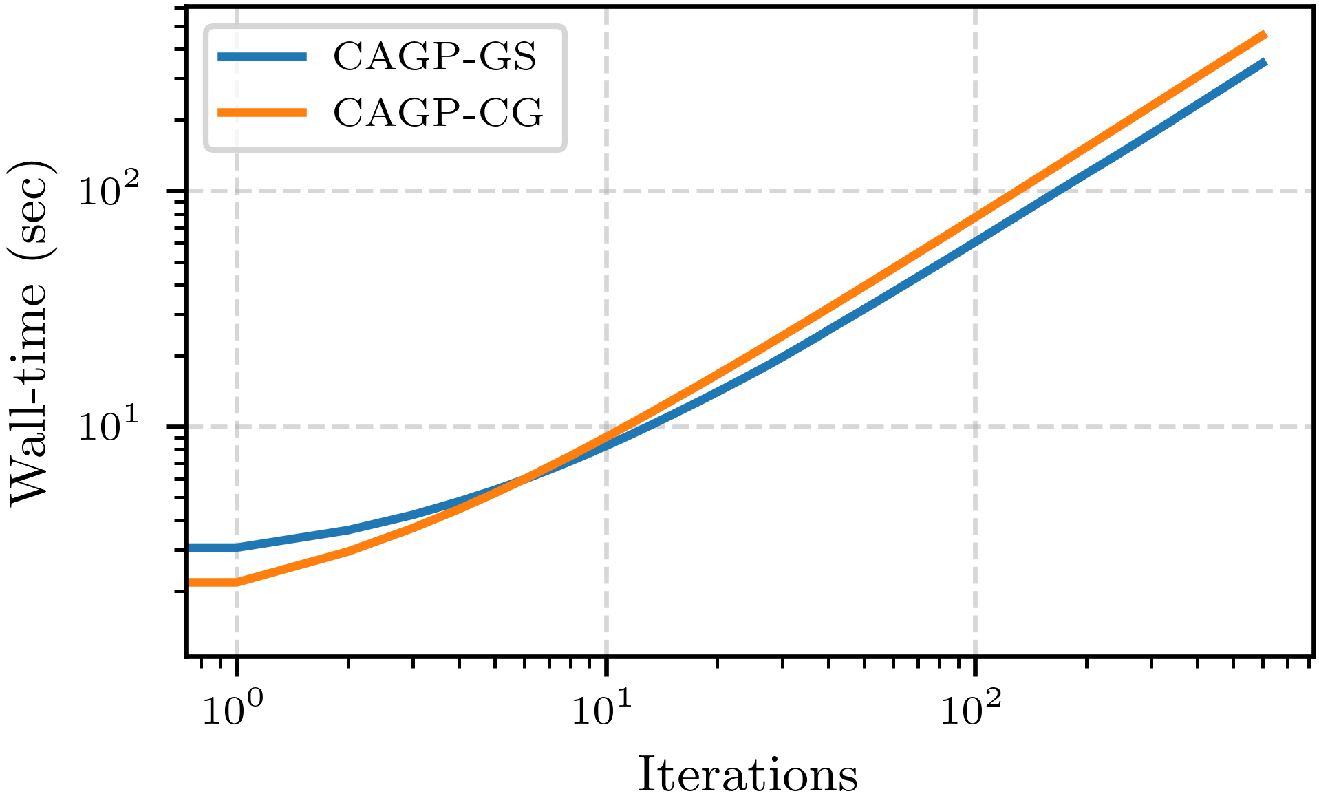
(a) Varying $m$.

(b) Varying $d$.

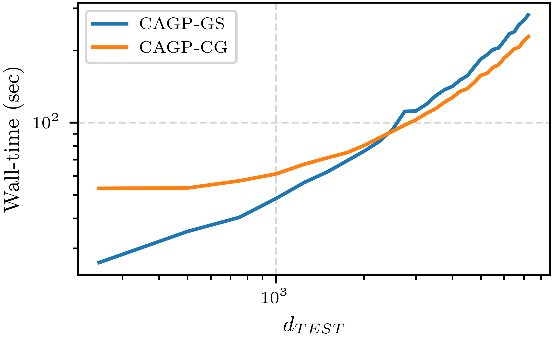
(c) Varying $d_{\textsc{test}}$.

Figure 4: Timings for the large-scale regression problem from Section 5.2 as a variety of parameters are varied.

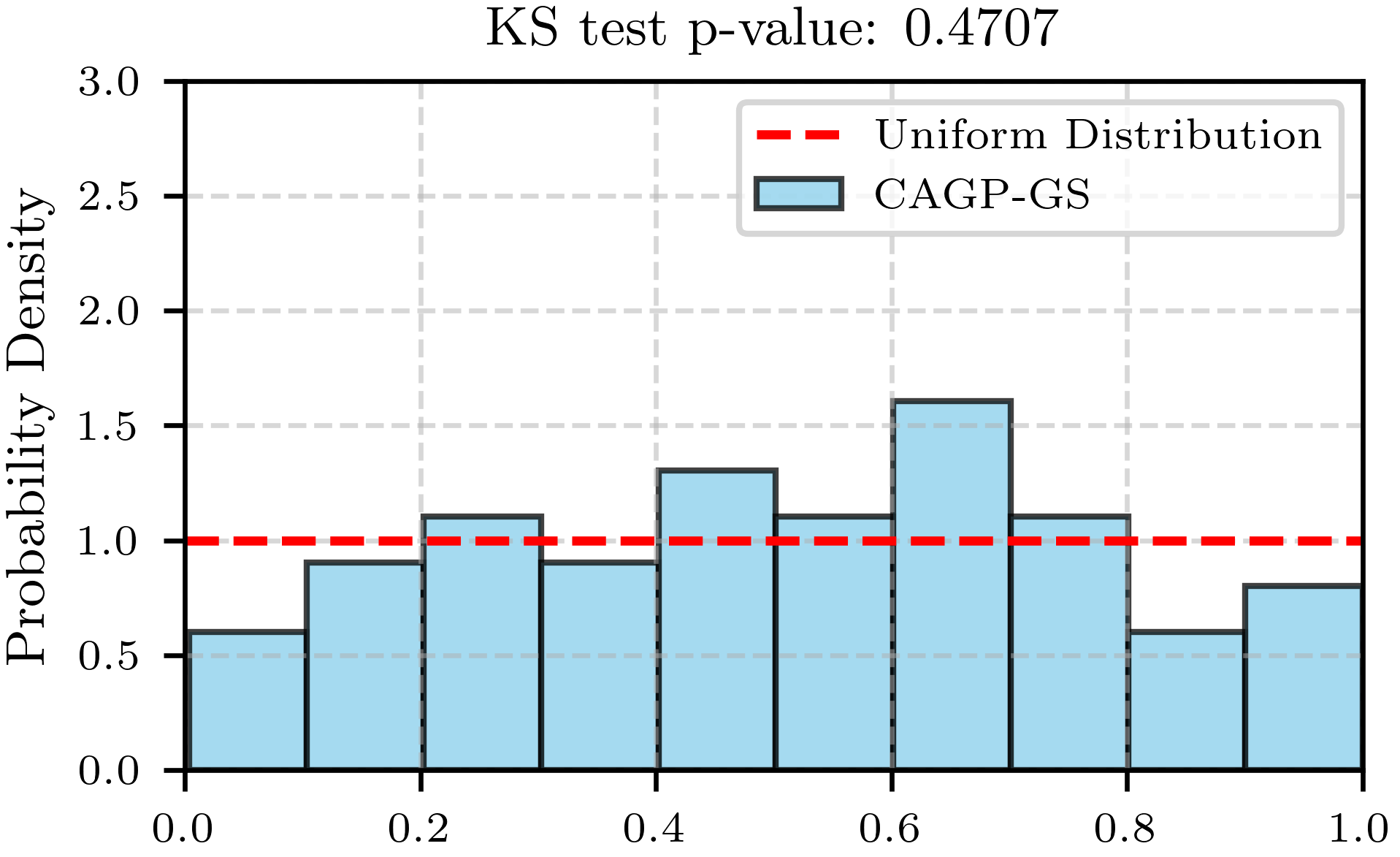
(a) CAGP-GS

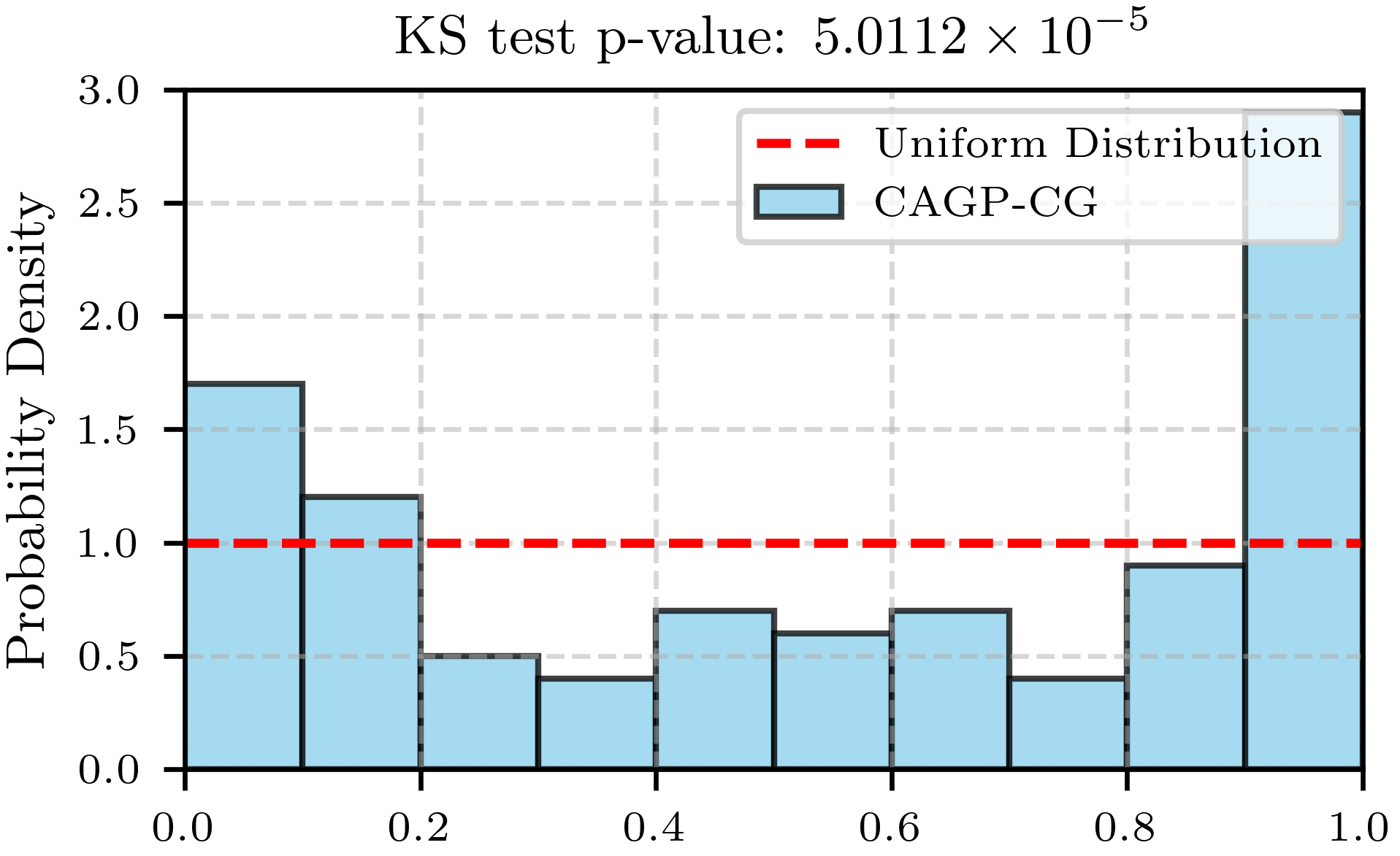
(b) CAGP-CG

Figure 5: Calibration results for the large-scale regression problem from Section 5.2

apalike

citations

References

- Bartels et al., (2019) Bartels, S., Cockayne, J., Ipsen, I. C. F., and Hennig, P. (2019). Probabilistic linear solvers: a unifying view. Statistics and Computing, 29(6):1249–1263.
- Cockayne et al., (2022) Cockayne, J., Graham, M. M., Oates, C. J., Sullivan, T. J., and Teymur, O. (2022). Testing whether a learning procedure is calibrated. Journal of Machine Learning Research, 23(203):1–36.
- Cockayne et al., (2021) Cockayne, J., Ipsen, I. C., Oates, C. J., and Reid, T. W. (2021). Probabilistic iterative methods for linear systems. Journal of Machine Learning Research, 22(232):1–34.
- (4) Cockayne, J., Oates, C. J., Ipsen, I. C. F., and Girolami, M. (2019a). A Bayesian conjugate gradient method (with discussion). Bayesian Anal., 14(3):937–1012. Includes 6 discussions and a rejoinder from the authors.
- (5) Cockayne, J., Oates, C. J., Sullivan, T. J., and Girolami, M. (2019b). Bayesian probabilistic numerical methods. SIAM Review, 61(3):756–789.
- Ferrari-Trecate et al., (1998) Ferrari-Trecate, G., Williams, C., and Opper, M. (1998). Finite-dimensional approximation of gaussian processes. In Advances in Neural Information Processing Systems, volume 11.
- Golub and Van Loan, (2013) Golub, G. H. and Van Loan, C. F. (2013). Matrix Computations. Johns Hopkins Studies in the Mathematical Sciences. Johns Hopkins University Press, Baltimore, MD, 4 edition.
- Gorodentsev, (2017) Gorodentsev, A. L. (2017). Algebra II: Textbook for Students of Mathematics. Springer International Publishing.
- Hennig et al., (2022) Hennig, P., Osborne, M. A., and Kersting, H. P. (2022). Probabilistic Numerics: Computation as Machine Learning. Cambridge University Press, Cambridge.
- Hersbach et al., (2023) Hersbach, H., Bell, B., Berrisford, P., Biavati, G., Horányi, A., Muñoz Sabater, J., Nicolas, J., Peubey, C., Radu, R., Rozum, I., Schepers, D., Simmons, A., Soci, C., Dee, D., and Thépaut, J.-N. (2023). ERA5 hourly data on single levels from 1940 to present. Accessed on 24-09-2020. Licence permits free use for any lawful purpose; see https://cds.climate.copernicus.eu/datasets/reanalysis-era5-single-levels for more details.
- Pförtner et al., (2024) Pförtner, M., Wenger, J., Cockayne, J., and Hennig, P. (2024). Computation-aware Kalman filtering and smoothing.
- Rasmussen and Williams, (2005) Rasmussen, C. E. and Williams, C. K. I. (2005). Gaussian Processes for Machine Learning. The MIT Press.
- Reid et al., (2022) Reid, T. W., Ipsen, I. C. F., Cockayne, J., and Oates, C. J. (2022). BayesCG as an uncertainty aware version of CG.
- Reid et al., (2023) Reid, T. W., Ipsen, I. C. F., Cockayne, J., and Oates, C. J. (2023). Statistical properties of BayesCG under the Krylov prior. Numer. Math., 155(3-4):239–288.
- Talts et al., (2018) Talts, S., Betancourt, M., Simpson, D., Vehtari, A., and Gelman, A. (2018). Validating bayesian inference algorithms with simulation-based calibration.
- Titsias, (2009) Titsias, M. (2009). Variational learning of inducing variables in sparse Gaussian processes. In van Dyk, D. and Welling, M., editors, Artificial intelligence and statistics, volume 5 of Proceedings of Machine Learning Research, pages 567–574.
- Wenger and Hennig, (2020) Wenger, J. and Hennig, P. (2020). Probabilistic linear solvers for machine learning. In Advances in Neural Information Processing Systems (NeurIPS), volume 33, pages 6731–6742.
- (18) Wenger, J., Pleiss, G., Hennig, P., Cunningham, J., and Gardner, J. (2022a). Preconditioning for scalable Gaussian process hyperparameter optimization. In International Conference on Machine Learning, volume 162 of Proceedings of Machine Learning Research, pages 23751–23780.
- (19) Wenger, J., Pleiss, G., Pförtner, M., Hennig, P., and Cunningham, J. P. (2022b). Posterior and computational uncertainty in Gaussian processes. In Advances in Neural Information Processing Systems (NeurIPS), volume 35, pages 10876–10890.
- Xu and Zikatanov, (2017) Xu, J. and Zikatanov, L. (2017). Algebraic multigrid methods. Acta Numerica, 26:591–721.
- Young, (1971) Young, D. M. (1971). Iterative Solution of Large Linear Systems. Academic Press.