Entanglement and coherence of the wobbling mode

Abstract

The entanglement and coherence of the wobbling mode are studied in the framework of the particle plus triaxial rotor model for the one-quasiparticle nucleus ¹³⁵Pr and the two-quasiparticles nucleus ¹³⁰Ba. The focus lies on the coupling between the total and the particle angular momenta. Using the Schmidt decomposing, it is quantified in terms of the von Neumann entropy of the respective sub-systems, which measures their mutual entanglement. The entropy and the entanglement increase with spin $I$ and number of wobbling quanta $n$. The coherence of the wobbling mode is studied by means of the eigenstate decomposition of its reduced density matrix. To a good approximation, the probability distributions of the total angular momentum can be interpreted as the incoherent combination of the coherent contributions from the first two pairs of eigenvectors with the largest weight of the reduced density matrix. Decoherence measures are defined, which, in accordance, scatter between 0.1 to 0.2 at low spin and between 0.1 and 0.3 at high spin. Entanglement in the framework of the adiabatic approximation is further analyzed. In general, the coherent eigenstates of the effective collective Hamiltonian approximate the reduced density matrix with the limited accuracy of its pair of eigenstates with the largest weight. As the adiabatic approximation becomes more accurate with decreasing excitation energy, the probability distribution of the angle of the total angular momentum around a principal axis approaches the one of the full reduced density matrix. The $E2$ transition probabilities and spectroscopic quadrupole moments reflect this trend.

I Introduction

The wobbling motion is a distinctive rotational mode indicating triaxiality within the nucleus Bohr and Mottelson (1975). A triaxial rotor prefers to rotate about the axis with the largest moment of inertia. When slightly excited, the rotational axis deviates from this principal axis, causing precession oscillations around the fixed angular momentum vector and resulting in the observed wobbling motion. This wobbling energy, characterized by the wobbling frequency, increases with the nuclear spin Bohr and Mottelson (1975).

In the study of triaxial rotors coupled with high-$j$ quasiparticles, Frauendorf and Dönau Frauendorf and Dönau (2014) categorized wobbling motions into two types: longitudinal wobbling (LW) and transverse wobbling (TW). LW occurs when the quasiparticle is mid-shell occupied, with its angular momentum $\bm{j}$ parallel to the principal axis of largest moment of inertia. TW, on the other hand, happens when the quasiparticle is bottom or top occupied, with its angular momentum $\bm{j}$ perpendicular to this axis. Both types show enhanced $I\to I-1$ electric quadrupole ($E2$) transitions between wobbling bands, characterized by rotational $E2$ bands corresponding to different oscillation quanta ($n$). LW’s wobbling frequency increases with spin, resembling the originally predicted wobbler behavior, while TW’s wobbling frequency decreases with spin. Later on, Chen and Frauendorf Chen and Frauendorf (2022) proposed a comprehensive classification of wobbling motion using spin coherent state (SCS) maps, which show the probability distribution for the orientation of angular momentum on the unit sphere projected onto the polar angle ($\theta$) and azimuthal angle ($\phi$) plane. In this scheme, LW involves the total angular momentum $\bm{J}$ revolving around the axis with the largest moment of inertia, while TW involves $\bm{J}$ revolving around an axis perpendicular to it. This classification is further validated by spin squeezed state (SSS) plots, linking discrete $\bm{J}$-space representation with the continuous coordinate $\phi$’s wave function Chen and Frauendorf (2024).

Experimental evidence of wobbling motion was first reported in triaxial strongly deformed nucleus ${}^{163}\textrm{Lu}$ in 2001 Ødegård et al. (2001), later interpreted as TW Frauendorf and Dönau (2014). The TW was also identified in the normally deformed nucleus ${}^{135}\textrm{Pr}$ Matta et al. (2015). The LW was observed in ${}^{187}\textrm{Au}$ Sensharma et al. (2020). As of now, wobbling candidate bands have been detected in over 15 nuclei across various mass regions Guo et al. (2024); Timár et al. (2019); Matta et al. (2015); Sensharma et al. (2019); Biswas et al. (2019); Petrache et al. (2019); Chen et al. (2019); Chakraborty et al. (2020); Rojeeta Devi et al. (2021); Lv et al. (2022); Prajapati et al. (2024); Ødegård et al. (2001); Jensen et al. (2002); Bringel et al. (2005); Schönwaßer et al. (2003); Amro et al. (2003); Hartley et al. (2009); Mukherjee et al. (2023); Sensharma et al. (2020); Nandi et al. (2020). A recent review is available in Refs. Frauendorf (2024); Sun et al. (2024).

Wobbling motion was initially predicted for even-even nuclei using the triaxial rotor model (TRM) Bohr and Mottelson (1975). After experimental confirmation in odd-$A$ nuclei Ødegård et al. (2001), the particle triaxial rotor (PTR) model became the primary framework for describing wobbling motion, including energy spectra and electromagnetic transitions Hamamoto (2002); Hamamoto and Mottelson (2003); Frauendorf and Dönau (2014); Streck et al. (2018); Chen et al. (2019, 2020); Broocks et al. (2021); Hu et al. (2021); Chen and Frauendorf (2022); Li et al. (2022); Dai et al. (2023); Li et al. (2024); Chen and Frauendorf (2024); Dai and Chen (2024). Additionally, several approximate methods have also been employed to study wobbling motion Tanabe and Sugawara-Tanabe (2017); Raduta et al. (2017); Budaca (2018); Lawrie et al. (2020); Budaca (2021); Raduta et al. (2021, 2022); Budaca and Petrache (2022). Different explanations for transverse wobbling motion have been proposed within these approaches Tanabe and Sugawara-Tanabe (2017); Lawrie et al. (2020). Moreover, the cranking model plus random phase approximation (RPA) Marshalek (1979); Shimizu and Matsuzaki (1995); Matsuzaki et al. (2002, 2004a); Matsuzaki and Ohtsubo (2004); Matsuzaki et al. (2004b); Shimizu et al. (2004, 2005); Almehed et al. (2006); Shimizu et al. (2008); Shoji and Shimizu (2009); Frauendorf and Dönau (2015) or collective Hamiltonian Chen et al. (2014, 2016), as well as the triaxial projected shell model Shimada et al. (2018); Wang et al. (2020); Chen and Petrache (2021) have been utilized to investigate and explain wobbling motion.

Within the framework of the PTR model, the phenomena of TW and LW have been interpreted as the interplay of one (or more) high-$j$ quasiparticle, which act as gyroscopes, and the remaining nucleons, which are modeled as a triaxial rotor. The PTR model describes this composite system using bases with good particle and total angular momentum and taking full account of the coupling between particle and rotor subsystems. In this work we will study the topological classification scheme suggested in Refs. Frauendorf and Dönau (2014); Chen and Frauendorf (2022, 2024) from the fundamental perspective of composite quantum systems. We will address the entanglement of the particle-rotor subsystems and the resulting limits of the interpretations based on the individual subsystems. Compared to other approaches, PTR is best suited for such a study because it is a simple two-component system. Previous studies have shown that the TW becomes unstable with increasing angular momentum Frauendorf and Dönau (2014); Matta et al. (2015); Streck et al. (2018); Chen and Frauendorf (2022); Li et al. (2024); Chen and Frauendorf (2024); Frauendorf (2024); Dai and Chen (2024). It changes into LW via a transition region. The variation is caused by the strong coupling between the angular momenta of the particles and the rotor. These are examples of strong entanglement between the particle and core angular momenta, well suited to quantify the entanglement and the resulting information loss in the case of wobbling motion.

Entanglement is a fundamental concept in quantum mechanics, which characterizes the correlations between particles or partitions within a composite system that cannot be described in terms of independent subsystems. Quantum many-body systems show specific signatures of entanglement, which are of great interest for condensed matter physics and quantum field theory Calabrese and Cardy (2004); Amico et al. (2008); Peschel and Eisler (2009); Horodecki et al. (2009); Nishioka et al. (2009); Eisert et al. (2010); Lin and Radičević (2020). Recent advances in quantum information science and quantum computing have renewed interest in exploring entanglement in nuclear systems Kanada-En’yo (2015a); Legeza et al. (2015); Kanada-En’yo (2015b, c); Beane et al. (2019); Robin et al. (2021); Faba et al. (2021); Kruppa et al. (2022); Pazy (2023); Bai and Ren (2022); Lacroix et al. (2022); Tichai et al. (2023); Bulgac et al. (2023); Bulgac (2023); Johnson and Gorton (2023); Gu et al. (2023).

The reduced density matrices for the total and particle angular momenta are the centerpieces of the tools introduced in Refs. Frauendorf and Dönau (2014); Chen and Frauendorf (2022, 2024) in order to elucidate the physics of the PTR system. The concept of the density matrix was introduced by John von Neumann von Neumann (1927) in order to establish a sound basis for the measuring process in quantum mechanics and by Lev Landau to extend the concept of Gibbs entropy from classical to quantum statistical mechanics Landau (1927). There are several entanglement measures based on the density matrix, which are commonly employed to quantify many-body correlations in quantum many-body systems. One such measure is the entropy of entanglement, also von Neumann (vN) entropy. This measure quantifies the extent of quantum entanglement between two subsystems within a composite quantum system. The vN entropy has been extensively employed in studies related to entanglement in the fields of condensed matter physics and quantum field theory Calabrese and Cardy (2004); Amico et al. (2008); Peschel and Eisler (2009); Horodecki et al. (2009); Nishioka et al. (2009); Eisert et al. (2010); Lin and Radičević (2020) and the atomic nuclei Kanada-En’yo (2015a); Legeza et al. (2015); Kanada-En’yo (2015b, c); Beane et al. (2019); Robin et al. (2021); Faba et al. (2021); Kruppa et al. (2022); Pazy (2023); Bai and Ren (2022); Lacroix et al. (2022); Tichai et al. (2023); Bulgac et al. (2023); Bulgac (2023); Johnson and Gorton (2023); Gu et al. (2023). In our study of entanglement in the wobbling motion, we will utilize the vN entropy to gain insights into the entanglement properties of the wobbling motion.

Spatial coherence is another important characteristics of entangled quantum systems Born et al. (1999). It measures the capability of waves propagating in a medium to generate interference pattern, which appear as a consequence of a definite relation between of the phase of the wave and the location in space Hecht (1998). A familiar example is the two-slit experiment monochromatic light. The two-dimensional waves behind the slits generate the interference pattern. For infinite narrow slits the interference fringes extend to infinity. In real systems they become weaker with the distance from the slits and eventually disappear over a distance called the coherence length. The reason for the damping is dephasing, which is the gradual loss of the definite relation between location and phase of the wave. There are various reasons for dephasing. The finite width of the slits is one of them. An incoherent mixture of different wave lengths is another. In analogy, the quantum wave function defines a unique phase difference between two points in space. A quantum system is called coherent when it can be described by wave function. Its “pure” density matrix is the product of the wave function with its complex conjugate. The general case are the “mixed” systems which are ensembles of such pure systems with different wave lengths such that the coherence is partially lost. We will address the loss of coherence in the particle-rotor system.

It has to be stressed that, although the entanglement causes the loss of coherence, the degree of it depends on the specific system. For example, the coupling of the electromagnetic field of the light wave with the degrees of freedom of the medium causes dephasing, the degree of which depends not only on the strength of the entanglement but also on the time scales of the involved degrees of freedom. Optical interference in glass with a high refraction index is an example for good coherence and substantial entanglement of the electric field with the atomic degrees of freedom of the glass. The phenomena can be very well described by the Maxwell equations in matter, which is an effective theory where the entanglement appears only in form of the permittivity and permeability of the material. In analogy, we address the question to what extend can the particle-rotor system understood in terms of an effective Hamiltonian in the orientation degrees of freedom of the total angular momentum only, so to speak a quasi-rotor. Such an approach is used in molecular physics to account for the coupling between the rotational and vibrational degrees of freedom, where effective rotor Hamiltonians with higher than two powers of the total angular momentum are introduced.

In this paper, we will investigate the entanglement entropy and coherence properties of the PTR model, using the nuclei ¹³⁵Pr studied in Refs. Frauendorf and Dönau (2014); Matta et al. (2015); Streck et al. (2018); Sensharma et al. (2019); Chen and Frauendorf (2022, 2024) and ¹³⁰Ba studied in Refs. Petrache et al. (2019); Chen et al. (2019); Chen and Frauendorf (2024) as examples for one- and two-quasiparticles coupled to a triaxial rotor.

II Theoretical framework

II.1 Particle triaxial rotor model

The PTR model is utilized to describe the coupling of a high-$j$ particle to a triaxial rotor core. The corresponding Hamiltonian can be expressed as Bohr and Mottelson (1975)

$$H_{\textrm{PTR}} =\hat{h}_{p}(\gamma)+\sum\limits_{i=1,2,3}\frac{(\hat{J}_{i}-\hat{j}_{i})^{2}}{2{\cal J}_{i}},$$ (1)

$$\hat{h}_{p}(\gamma) =\kappa\left[\left(3\hat{j}_{3}^{2}-\bm{j}^{2}\right)\cos\gamma+\sqrt{3}\left(\hat{j}_{1}^{2}-\hat{j}_{2}^{2}\right)\sin\gamma\right],$$ (2)

Here, $\hat{J}_{i}=\hat{R}_{i}+\hat{j}_{i}$ represents the total angular momentum, where $\hat{j}_{i}$ corresponds to the angular momentum of the particle and $\hat{R}_{i}$ represents the angular momentum of the triaxial rotor. The ${\cal J}_{i}$ denotes the moment of inertia along the $i$ axis, which is dependent on the deformation parameters $\beta$ and $\gamma$. The single-particle Hamiltonian $h_{p}(\gamma)$ takes into account the coupling strength to the deformed potential, and is expressed as a function of $\gamma$, with $\kappa$ representing the coupling strength constant.

The PTR Hamiltonian (1) can be decomposed into four parts

$$\hat{H}_{\textrm{PTR}}=\hat{h}_{p}(\gamma)+\hat{H}_{\textrm{rot}}+\hat{H}_{\textrm{rec}}+\hat{H}_{\textrm{cor}},$$ (3)

with the pure rotational operator of the rotor

$$\hat{H}_{\textrm{rot}}=\sum_{i=1,2,3}\frac{\hat{J}_{i}^{2}}{2{\cal J}_{i}},$$ (4)

the recoil term

$$\hat{H}_{\textrm{rec}}=\sum_{i=1,2,3}\frac{\hat{j}_{i}^{2}}{2{\cal J}_{i}},$$ (5)

and the Coriolis interaction term

$$\hat{H}_{\textrm{cor}}=-\sum_{i=1,2,3}\frac{\hat{J}_{i}\hat{j}_{i}}{{\cal J}_{i}},$$ (6)

of which $H_{\textrm{rot}}$ acts only on the degrees of freedom of the rotor and $H_{\textrm{rec}}$ acts in the coordinates of the valence particle only, whereas $H_{\textrm{cor}}$ couples the degrees of freedom of the rotor to the degrees of freedom of the valence particle. Therefore, the entanglement between the rotor and the valence particle is generated only by the $H_{\textrm{cor}}$.

The PTR Hamiltonian is diagonalized in the product basis $|IIK\rangle|jk\rangle$, where $|IIK\rangle$ represents rotor states with half-integer $I$ and $|jk\rangle$ the high-$j$ particle states in good spin $j$ approximation. The eigenstates of the PTR Hamiltonian are expressed as

$$|II,\nu\rangle=\sum_{K,k}C_{IKk}^{(I\nu)}|IIK\rangle\otimes|jk\rangle,$$ (7)

in terms of the coefficients $C_{IKk}^{(I\nu)}$. Here, $K$ and $k$ run respectively from $-I$ to $I$ and from $-j$ to $j$. The coefficients are restricted by the requirement that collective rotor states must be symmetric representations of the D₂ point group. This implies that the difference $K-k$ must be even and one-half of all coefficients is fixed by the symmetric relation

$$C_{I-K-k}^{(I\nu)}=(-1)^{I-j}C_{IKk}^{(I\nu)}.$$ (8)

The generalization to the two-quasiparticle triaxial rotor model is straightforward,

$$|II,\nu\rangle=\sum_{K,k_{1},k_{2}}C_{IKk_{1}k_{2}}^{(I\nu)}|IIK\rangle\otimes|jk_{1}\rangle\otimes|jk_{2}\rangle,$$ (9)

where $|IIK\rangle$ represents rotor states with integer $I$. Here, both $k_{1}$ and $k_{2}$ run from $-j$ to $j$. The D₂ symmetry implies that the difference $K-k_{1}-k_{2}$ must be even and one-half of all coefficients is fixed by the symmetric relation

$$C_{I-K-k_{1}-k_{2}}^{(I\nu)}=(-1)^{I-2j}C_{IKk_{1}k_{2}}^{(I\nu)},$$ (10)

and the Pauli exclusion principle

$$C_{IKk_{1}k_{2}}^{(I\nu)}=-C_{IKk_{2}k_{1}}^{(I\nu)}.$$ (11)

From the amplitudes of the eigenstates $C_{IKk}^{(I\nu)}$, we can calculate the reduced density matrices, as described in Refs. Chen and Frauendorf (2022, 2024). The reduced density matrices provide valuable information about the particle angular momentum $\bm{j}$ and the total angular momentum $\bm{J}$. Specifically, we have the reduced density matrices for the particle angular momentum states $|j\rangle$

$$\rho_{kk^{\prime}}^{(I\nu)}=\sum_{K}C_{IKk}^{(I\nu)}C_{IKk^{\prime}}^{(I\nu)*},$$ (12)

and for the total angular momentum states $|II\rangle$

$$\rho_{KK^{\prime}}^{(I\nu)}=\sum_{k}C_{IKk}^{(I\nu)}C_{IK^{\prime}k}^{(I\nu)*}.$$ (13)

Similarly, for the two-quasiparticle triaxial rotor model, we can also calculate the reduced density matrix from the eigenstates $C_{IKk_{1}k_{2}}^{(I\nu)}$ for the total particle angular momentum states $|j_{12}\rangle=|j\rangle\otimes|j\rangle$

$$\rho_{k_{12},k_{12}^{\prime}}^{(I\nu)} =\sum_{j_{12},K}C_{j_{12},k_{12},K}^{(I\nu)}C_{j_{12},k_{12}^{\prime},K}^{(I\nu)*},$$ (14)

$$C_{j_{12},k_{12},K}^{(I\nu)} =\sum_{k_{1},k_{2}}\langle jk_{1}jk_{2}|j_{12}k_{12}\rangle C_{IKk_{1}k_{2}}^{(I\nu)},$$ (15)

and for the total angular momentum states $|II\rangle$

$$\rho_{KK^{\prime}}^{(I\nu)}=\sum_{k_{1}k_{2}}C_{IKk_{1}k_{2}}^{(I\nu)}C_{IK^{\prime}k_{1}k_{2}}^{(I\nu)*}.$$ (16)

The reduced density matrices contain the information about the distribution and correlations of angular momenta within the system, which are the basis for interpreting the properties and behavior of triaxial nuclei by means of the PTR model Chen and Frauendorf (2022, 2024). They describe “what the particle and the total angular momentum vectors are doing”. The reduced density matrices represent mixed states. In the following we analyse the mutual entanglement of the particle and rotor subsystems, which results in a partial loss coherence in each partition.

II.2 Schmidt decomposition

The PTR model introduces a bipartition of the of the system into the two subsystems of the orientation of the total angular momentum $|IIK\rangle$ and of the orientation of the particle $|jk\rangle$. The Hilbert space of the PTR model is the direct product of the Hilbert spaces of the two subsystems, $\mathcal{H}_{Kk}=\mathcal{H}_{K}\otimes\mathcal{H}_{k}$. The Schmidt decomposition (equivalent to the singular value decomposition of a matrix) Nielsen and Chuang (2010) diagonalizes the two reduced density matrices in their respective subspaces,

$$\rho_{KK^{\prime}}=\sum_{m}p_{m}C^{(m)}_{IK}C^{(m)}_{IK^{\prime}},$$ (17)

where $p_{m}$ are the eigenvalues and $C^{(m)}_{IK}$ are the normalized eigenvectors;

$$\rho_{kk^{\prime}}=\sum_{m}p_{m}C^{(m)}_{k}C^{(m)}_{k^{\prime}},$$ (18)

where $p_{m}$ are the eigenvalues and $C^{(m)}_{k}$ are the normalized eigenvectors. For the case that the dimension $d_{j}$ of the $\bm{j}$-space is smaller than dimension $d_{J}$ of the $\bm{J}$-space, the first $d_{j}$ eigenvalues $p_{m}$ of $\rho_{KK^{\prime}}$ are the same as the $p_{m}$ for $\rho_{kk^{\prime}}$, and the remaining $p_{m}=0$. For $d_{J}<d_{j}$ it is the other way around. The $p_{m}$ satisfy the normalization condition

$$\sum_{m}p_{m}=1.$$ (19)

If $p_{1}=1$ and $p_{m>1}=0$ the system is in a pure state. The particle and the total angular momentum are described by the eigenstates

$$|II,1\rangle=\sum_{K}C_{IK}^{(1)}|IIK\rangle,\quad|j,1\rangle=\sum_{k}C_{k}^{(1)}|jk\rangle.$$ (20)

The two subsystems are separate, the combined state is the product of the substates. This corresponds to the frozen alignment (FA) approximation introduced in Ref. Frauendorf and Dönau (2014).

If some $p_{m}\neq 1$ the two subsystems are no longer independent. They are said to be entangled, where $p_{m}$ represents the probability for the subsystems to be in one of the pure states $|II,m\rangle$ and $|j,m\rangle$ and the total system being in the product state of both. In the following we discuss various measures that quantify the degree and characteristics of the entanglement.

II.3 Entropy

The vN entropy von Neumann (1927) proved to be an appropriate entanglement measure in quantum many-body systems (see, for instance, Refs. Amico et al. (2008); Tichy et al. (2011) and references therein). It characterizes the lack of complete information about a subsystem when the total system is a known pure state. In our case the bipartition concerns the total ($\bm{J}$) and proton ($\bm{j}$) angular momenta.

The vN entropy, also called “entanglement entropy”, is defined by either of the reduced density matrices

$$S_{j(J)}=-\textrm{Tr}~{}\rho_{j(J)}\ln\rho_{j(J)}=-\sum_{m}p_{m}\ln p_{m}.$$ (21)

It quantifies the ignorance due to the correlation between subsystems $\bm{j}$ and $\bm{J}$ Vedral et al. (1997). As it characterizes the relation between the subsystems, it is the same for either of them. In information theory the last expression in (21) is also called the Shannon entropy. They use the $\log$ in base 2, which is the natural unit for the binary digit.

The entanglement entropy measures how correlated (“entangled”) the two sectors are. If there is no entanglement between the two subsystems, we find $S=0$; and $S>0$ if there is entanglement. Any subsystem eigenstate which has $p_{m}=0$ or $p_{m}=1$ will not contribute to the entropy.

Without the Coriolis interaction, $\mathcal{H}_{K}$ and $\mathcal{H}_{k}$ are decoupled. The entropy takes its minimum

$$S^{(\textrm{min})}=\left\{\begin{array}[]{ll}0,&\textrm{for even-even},\\ \ln{2},&\textrm{for odd-}A,\\ \ln{4},&\textrm{for odd-odd}.\end{array}\right.$$ (25)

The reason for the difference is Kramer’s degeneracy. The single-particle Hamiltonian $\hat{h}_{p}(\gamma)$ couples only states that differ by $\Delta k=2$. For the even-even system the eigenstates have either even-$k$ or odd-$k$. The energies of the two sets are different, though not very. That is, the eigenstates are pure and their entropy is $S^{(\textrm{min})}=0$. In the case of odd-$A$, the eigenstates of $\hat{h}_{p}(\gamma)$ have $k=j+\textrm{even}$ (labeled as $|\varphi\rangle$) or $k=-j+\textrm{even}$ (labeled as $|\bar{\varphi}\rangle$), which have the same energy (Kramer’s degeneracy). Coupling matrix elements between the two classes will generate superpositions $(|\varphi\rangle\pm|\bar{\varphi}\rangle)/\sqrt{2}$. This has the consequence that the eigenvalues of the $\bm{j}$-density matrix come in doublets. Approaching the limit of zero Coriolis interaction, there are two eigenvalues of 1/2 and the rest is zero, because any whatsoever small coupling will generate the superposition. Thus we consider $S^{(\textrm{min})}=\ln 2$ as the minimal entropy, which is also the result of the numerical calculations.

If the reduced $\bm{j}$-density matrix is given by the normalized identity matrix $\rho_{kk^{\prime}}=\delta_{kk^{\prime}}/d_{j}$, then the vN entropy reaches the maximal value

$$S_{j}^{(\textrm{max})}=\ln~{}d_{j}.$$ (26)

In this limit the subsystems $\bm{j}$ and $\bm{J}$ are maximally entangled. Each state $|jk\rangle$ is realized with the same probability $1/d_{j}$, that is, there is maximal randomness. The SSS plot Chen and Frauendorf (2024) is the straight line $P(\phi)=1/2\pi$.

The entropy of the $\bm{J}$-subsystem is $\ln~{}d_{j}$ as well, because the $p_{m}$ are the same or 0. However, in units of the maximal possible $\bm{J}$-entropy (i.e., complete randomness), $S_{J}^{(\textrm{max})}=\ln~{}d_{J}$, it is smaller than one ($\ln~{}d_{j}/\ln~{}d_{J}<1$). Accordingly, the $\bm{J}$-density matrix (17) with $p_{m}=1/d_{j}$ for $m\leq d_{j}$ and 0 $m>d_{j}$ is not diagonal in $K,~{}K^{\prime}$. The pertaining SSS plot Chen and Frauendorf (2024) shows quantum fluctuations. The random motion of the particle cannot completely randomize the total angular momentum orientation with respect to the principal axes.

The limit of complete randomness of a small subsystem is approached by strongly coupling it to a large subsystem, which acts as a randomizing heat bath. This scenario differs from the $\bm{j}$-$\bm{J}$ subsystems of the PTR. As discussed below, $S$ stays well below its maximum for all states.

II.4 Purity

Furthermore, we calculate the purity, which is a measure on quantum states on how much a state is mixed. It is defined as

$$\mathcal{P}=\textrm{Tr}~{}\rho^{2}=\sum_{m}p_{m}^{2},$$ (27)

with $p_{m}$ being the eigenvalues of $\rho$. When it is 1, the state is pure. Otherwise, it will be smaller than 1, with the minimum $1/d_{j}$ for the particle or total angular momenta. Because of Kramer’s degeneracy, the maximal purity is 1/2 in the case of odd-$A$.

II.5 Coherence

“Coherence” specifies to which extend the system can be described by wave function with the characteristic interference phenomena. If the system is pure, i.e., it is represented by only one wave function in $K$-space, then one has

$$\left[\rho^{(I\nu)}\right]^{2}_{KK^{\prime}} =\sum\limits_{K^{\prime\prime}=-I}^{I}\rho^{(I\nu)}_{KK^{\prime\prime}}\rho^{(I\nu)}_{K^{\prime\prime}K^{\prime}}$$

$$=\sum\limits_{K^{\prime\prime}=-I}^{I}C_{IK}^{(I\nu)}C_{IK^{\prime\prime}}^{(I\nu)*}C_{IK^{\prime\prime}}^{(I\nu)}C_{IK^{\prime}}^{(I\nu)*}$$

$$=C_{IK}^{(I\nu)}C_{IK^{\prime}}^{(I\nu)*}$$

$$=\rho^{(I\nu)}_{KK^{\prime}},$$ (28)

which indicates complete coherence. For mixed states, this relation no longer holds. In order to measure the loss of coherence, it is natural to ask how the square of the density matrix deviates from the matrix. One thus considers the matrix square as a modified density matrix and asks how it deviates from the original one. However, the trace of the squared matrix is smaller than 1, where the reduction measures the purity. For a proper comparison, the squared matrix must be normalized by dividing it by its trace. We compare the $K$-probability distributions and use the absolute deviation $\Delta_{K}$ as a measure for decoherence. It turns out that the deviations depend to some extend on the representation of the density matrix. The corresponding formula are given as

$$P(K) =\rho^{(I\nu)}_{KK},$$ (29)

$$P_{2}(K) =\left[\rho^{(I\nu)}\right]^{2}_{KK}/\mathrm{Tr}\left\{\left[\rho^{(I\nu)}\right]^{2}\right\},$$ (30)

$$\Delta_{K} =\sum_{K=-I}^{I}\Big{|}P_{2}(K)-P(K)\Big{|}.$$ (31)

Here, we use the absolute value instead of the root-mean-squared of the difference between the $P(K)$ and $P_{2}(K)$ in calculating $\Delta_{K}$, because the latter does not fulfill the “continuity criterion” for a coherence measure Baumgratz et al. (2014).

The analogue comparison can be based on the spin squeezed state (SSS) plots Chen and Frauendorf (2024). They represent the $K$-space in terms of a continuous coordinate $\phi$, which represents the angle between the projection of $\bm{J}$ onto the short-medium ($sm$) plane with the short ($s$) axis of the triaxial nuclear shape. Mathematically, one changes to the Fourier representation of the density matrix

$$\rho_{\phi,\phi^{\prime}}^{(I\nu)} =\frac{1}{2\pi}\sum\limits_{K,K^{\prime}=-I}^{I}\rho^{(I\nu)}_{KK^{\prime}}e^{-i(K\phi-K^{\prime}\phi^{\prime})},$$ (32)

$$\left[\rho^{(I\nu)}\right]^{2}_{\phi,\phi^{\prime}} =\frac{1}{2\pi}\int_{-\pi}^{\pi}d\phi^{\prime\prime}\rho_{\phi,\phi^{\prime\prime}}^{(I\nu)}\rho_{\phi^{\prime\prime},\phi^{\prime}}^{(I\nu)}$$

$$=\frac{1}{2\pi}\sum_{K,K^{\prime},K^{\prime\prime}=-I}^{I}\rho^{(I\nu)}_{KK^{\prime\prime}}\rho^{(I\nu)}_{K^{\prime\prime}K^{\prime}}e^{-i(K\phi-K^{\prime}\phi^{\prime})}.$$ (33)

As a result, the decoherence is quantified by

$$P(\phi) =\rho_{\phi,\phi}^{(I\nu)},$$ (34)

$$P_{2}(\phi) =\left[\rho^{(I\nu)}\right]^{2}_{\phi,\phi}/\mathrm{Tr}\left\{\left[\rho^{(I\nu)}\right]^{2}\right\},$$ (35)

$$\Delta_{\textrm{SSS}} =\int_{-\pi}^{\pi}d\phi~{}\Big{|}P_{2}(\phi)-P(\phi)\Big{|}.$$ (36)

The normalized $P_{2}$ distributions have the eigenvalues $p_{m}^{2}/\sum_{m^{\prime}}p_{m^{\prime}}^{2}$ $(m\geq 1)$. The ratio $p_{m}/p_{1}$ determines the probabilities of the incoherent terms for the distribution $P$. The ratio $(p_{m}/p_{1})^{2}$ determines the probability of the incoherent terms for the distribution $P_{2}$. As $(p_{m}/p_{1})^{2}<p_{m}/p_{1}$, the distribution $P_{2}$ is purer than $P$. The expressions (31) and (36) measure how the admixture of the $m>1$ modify the functions $P(K)$ and $P(\phi_{J})$. It depends on the relative phases of the eigenstates $C_{IK}^{(m)}$ of the reduced density matrix to which degree their combination suppresses the quantal oscillations, that is causes decoherence.

Furthermore, the Ref. Baumgratz et al. (2014) introduced the $l_{1}$ norm

$$C_{l_{1}}=\sum_{K\neq K^{\prime}}|\rho^{(I\nu)}_{KK^{\prime}}|$$ (37)

as a measure of coherence, which quantifies how sparse the density matrix is. This quantity has a simple intuitive form which is directly connected to the off-diagonal elements of $\rho$ in the basis $|K\rangle$ of interest. The rational behind it is that adding the contributions from eigenstates $|m\rangle$ with very different phases will reduce the absolute values the non-diagonal matrix elements. According to this measure, a diagonal density matrix is completely incoherent. The maximum of the $C_{l_{1}}^{(\textrm{max})}=d-1=2I$ Baumgratz et al. (2014), which corresponds to the absolute value of all matrix elements being equal to $1/d$. The density matrix of the pure state with the amplitudes $1/\sqrt{d}$ is an example. As for the above discussed expressions, the value of the $C_{l_{1}}$ norm depends on the chosen basis.

Since the coherence measures depend on the representation, we also calculate the $C_{l_{1}}$ norm for the reduced density matrix in the discrete SSS representation

$$C_{l_{1}} =\sum_{m\neq n}|\rho^{(I\nu)}_{\phi_{m},\phi_{n}}|,$$ (38)

$$\rho^{(I\nu)}_{\phi_{m},\phi_{n}} =\sum_{l}p_{l}C_{Im}^{(l)*}C_{In}^{(l)},$$ (39)

in which $C_{Im}^{(l)}$ denotes the normalized eigenvectors of the reduced density matrix in the discrete SSS representation. It is related to $C_{IK}^{(l)}$ by the transformation

$$C_{Im}^{(l)}=\frac{1}{\sqrt{2I+1}}\sum\limits_{K=-I}^{I}e^{iK\phi_{m}}C_{IK}^{(l)},$$ (40)

with $\phi_{m}=2\pi m/(2I+1)$, where $m=-I$, $-I+1$, …, $I$.

In this work, we will compare the qualities of coherence obtained from the $K$-plots and SSS-plots.

III Numerical details

First, we will discuss the entanglement entropy and coherence of the PTR model using ¹³⁵Pr studied in Refs. Frauendorf and Dönau (2014); Matta et al. (2015); Streck et al. (2018); Sensharma et al. (2019); Chen and Frauendorf (2022, 2024) as the first example for TW of triaxial nuclei with normal deformation. The parameters of the PTR are $\beta=0.17$ (corresponds to $\kappa=0.038$), $\gamma=-26^{\circ}$, and $\mathcal{J}_{m,s,l}=21$, 13, $4~{}\hbar^{2}/\textrm{MeV}$ for medium ($m$), short ($s$), long ($l$) axes, respectively. A comparison of the PTR results with the experimental energies and transition probabilities can be found in Refs. Frauendorf and Dönau (2014); Matta et al. (2015); Streck et al. (2018); Sensharma et al. (2019); Chen and Frauendorf (2022, 2024). Then, we will discuss the entanglement entropy and coherence for a two-quasiparticle triaxial rotor system using ¹³⁰Ba studied in Ref. Chen et al. (2019) as example. The deformation parameters are $\beta=0.24$ (corresponds to $\kappa=0.055$), $\gamma=21.5^{\circ}$ and the three spin-dependent moments of inertia $\mathcal{J}_{i}=\Theta_{i}(1+cI)$ are determined by the parameters $\Theta_{s,m,l}=1.09$, 1.50, and 0.65 $\hbar^{2}/\textrm{MeV}$ and $c=0.59$. A comparison of the PTR results with the experimental energies and transition probabilities can be found in Ref. Chen et al. (2019).

IV Wobbling modes

IV.1 Excitation energy

Figure 1(a) compares the excitation energies $\Delta E_{n}=E_{n}-\bar{E}_{n=0}$ of the wobbling bands with different wobbling numbers $n=1$, 2, and 3 in ¹³⁵Pr. The $n=0$ zero-wobbling energies $\bar{E}_{n=0}$ are equal to $E_{\textrm{yrast}}(I)$ for the signature $I=11/2+\textrm{even}$ and $[E_{\textrm{yrast}}(I-1)+E_{\textrm{yrast}}(I+1)]/2$ for the signature $I=13/2+\textrm{even}$. The states are labelled by the wobbling number $n$. However, this labelling does not imply that the wobbling motion is harmonic. In our previous studies Chen and Frauendorf (2022, 2024), we have classified the structure of the states as follows

• $I\leq 23/2$ is the transverse wobbling (TW) region. The total angular momentum of the nucleus precesses around the $s$ axis.

• $I=27/2$-$35/2$ is the flip region. The total angular momentum is tilted into the $sm$ plane about halfway between the two axes and jumps between the orientations of $s$ and $m$ axes.

• $I\geq 37/2$ is the longitudinal wobbling (LW) region. The total angular momentum of the nucleus precesses around the medium axis.

The three rotational modes are delineated by different background colors in Fig. 1.

Figures 2 and 3 illustrate the structure of the PTR states in ¹³⁵Pr by by showing, respectively, the probability distributions $P(K)$ of the projection of the total angular momentum onto the $l$ axis and $P(\phi_{J})$ of the angle of its projection onto the $sm$ plane with the $s$ axis. Both visualizations of the structure were introduced in our previous work Chen and Frauendorf (2022, 2024), where the details were given.

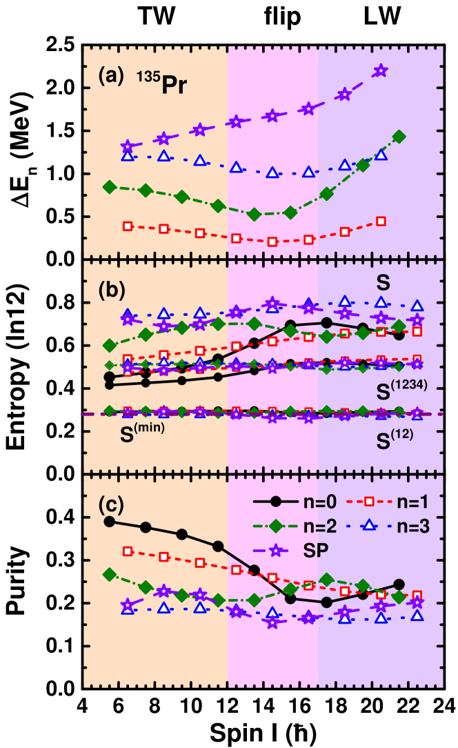
Figure 1: (Color online) (a) Excitation energies of the wobbling bands with wobbling numbers $n=1$, 2, and 3 and signature band with respect to the zero wobbling energy $\bar{E}_{\textrm{yrast}}(I)$ calculated by the PTR for ¹³⁵Pr. Note that the states in the wobbling bands are labelled by the wobbling quantum number $n$. (b) The entropy of the states $S$, $S^{(12)}$, and $S^{(1234)}$ in units of the maximal entropy $S_{j}^{(\textrm{max})}=\ln 12$. The dash-dot-dot line gives minimal entropy $S^{\textrm{(min)}}=\ln 2/\ln 12\approx 0.28$. (c) The purity of the states. The different backgrounds delineate the regions of the TW, flip, and LW modes.

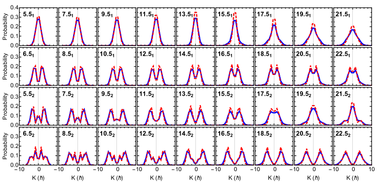
Figure 2: (Color online) Probability distribution of the total angular momentum projection on the $l$ axis for the $n=0$-$3$ states in ¹³⁵Pr calculated by PTR. Full curves show the one calculated by $P(K)$, while the dashed curves display the one by $P_{2}(K)$. Only the region $-9.5\leq K\leq 9.5$ is shown.

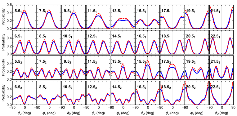
Figure 3: (Color online) Full curves show the probability density of the SSS $P(\phi_{J})$ for the $n=0$-$3$ states in ¹³⁵Pr calculated by PTR model, while the dashed curves display the $P_{2}(\phi_{J})$.

As discussed in detail there, the $n=0$ and 1 bands display a well defined wobbling structure. In the TW regime, its excitation energy $\Delta E_{n=1}$ decreases as the angular momentum $I$ increases up to $I=29/2$, which indicates that the collective wobbling motion becomes less and less stable. Subsequently, the TW regime transitions into a flip mode and then into a LW regime. This evolution is accompanied by a change to an increase of the excitation energy with increasing spin, which indicates that the collective motion becomes more stable again, resulting from a reduction in the amplitude of the wobbling motion.

The $n=2$ states exhibit significant deviations from the expected distributions of the harmonic limit, but still show the three peaks, which qualify them as distorted $n=2$ TW states Chen and Frauendorf (2022, 2024). As seen in Fig. 1(a), their excitation energies deviate from being twice the ones of the $n=1$ ones at high spin. As the angular momentum $I$ increases, the $n=2$ states undergo a transition into unharmonic two-wobbling LW structures.

The structure of the $n=3$ states structure differs qualitatively from the pattern expected for the unharmonic $n=3$ wobbling motion Chen and Frauendorf (2022, 2024). It has a flip structure already at the beginning of the band. The total angular momentum in the $n=3$ band mainly aligns along the $m$ axes. In addition, in the low spin region, it has admixture with the signature partner (SP) band. In the high spin region, it crosses with the $n=2$ band.

In addition, the excitation energy of SP band is also presented in Fig. 1(a). It increases with spin and is larger than the wobbling energies.

IV.2 Angular momentum

From the $k$-distribution and $K$-distribution plots, one can calculate the square roots of expectation values of the squares of angular momentum components for the particle and the total nucleus, respectively Chen and Frauendorf (2022). Figure 4 shows corresponding results for the $n=0$, 1, 2, and 3 wobbling bands in ¹³⁵Pr. The triaxial rotor is coupled with an $h_{11/2}$ proton. The $s$ axis is the preferred orientation, because it maximizes the overlap of the particle orbit with the triaxial core Frauendorf and Meng (1996). The rotation energy of the rotor core prefers the medium axis with the largest moment of inertia. At low spin $I$, the torque of the quasiparticle wins. The orientation of $\bm{J}$ and $\bm{j}$ along the $s$ axis represents the stable configuration. The growth of total angular momentum $\bm{J}$ is generated by an increase of the rotor angular momentum along the $s$ axis. Above the critical angular momentum the torque of the rotor core takes over. The total angular momentum moves into the $sm$ plane. The growth of total angular momentum $\bm{J}$ is essentially generated by an increase the rotor angular momentum along the medium axis. The particle angular momentum $\bm{j}$ is pulled toward to mdium axis because the Coriolis force tries to minimize the angle between $\bm{j}$ and $\bm{I}$. However, it does not align with the medium axis for the considered values of $I$ Chen and Frauendorf (2022).

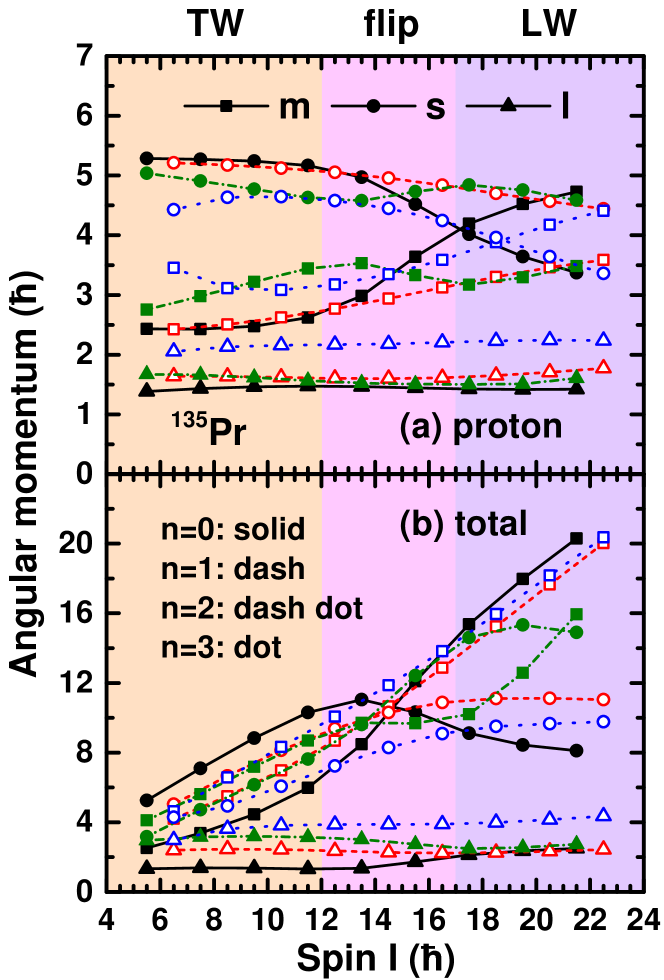
Figure 4: (Color online) Root mean square expectation values of the angular momentum components of the (a) proton and (b) total nucleus for the $n=0$, $1$, $2$, and $3$ bands in ¹³⁵Pr calculated by the PTR model.

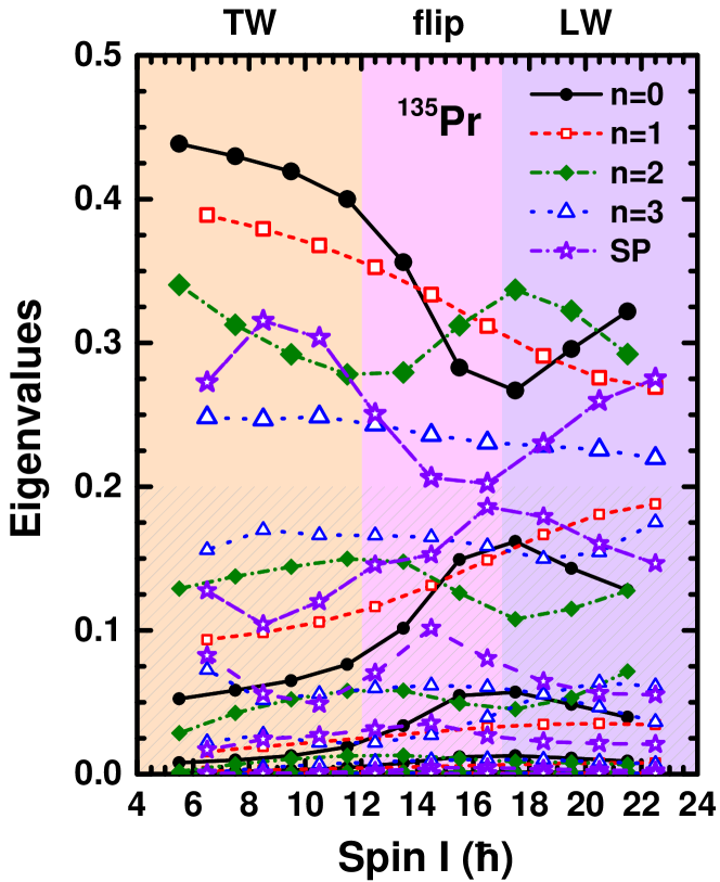
Figure 5: (Color online) Eigenvalues of the reduced density matrices of ¹³⁵Pr as functions of spin for the $n=0$, $1$, $2$, and $3$ and SP states. The slant shadow denotes the eigenvalues below 0.2.

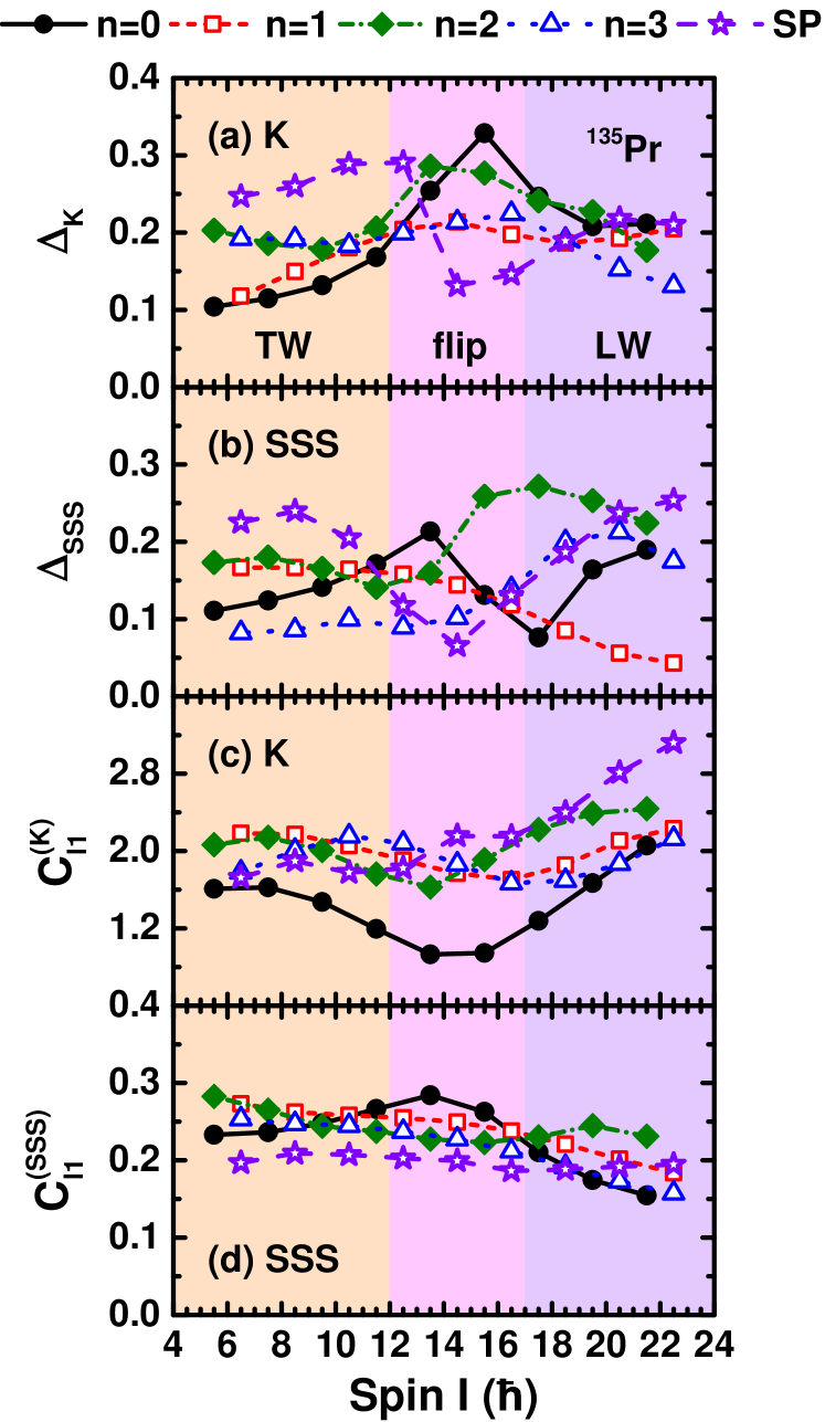
Figure 6: (Color online) The absolute deviations $\Delta_{K}$ (a) and $\Delta_{\textrm{SSS}}$ (b) as well as the $l_{1}$ norm $C_{l_{1}}^{(K)}$ (c) and $C_{l_{1}}^{(\textrm{SSS})}$ (d) of the $K$ distributions $P(K)$ and SSS plots $P(\phi_{J})$ as measures of decoherence for the $n=0$-$3$ states and signature partner band in ¹³⁵Pr calculated by PTR model.

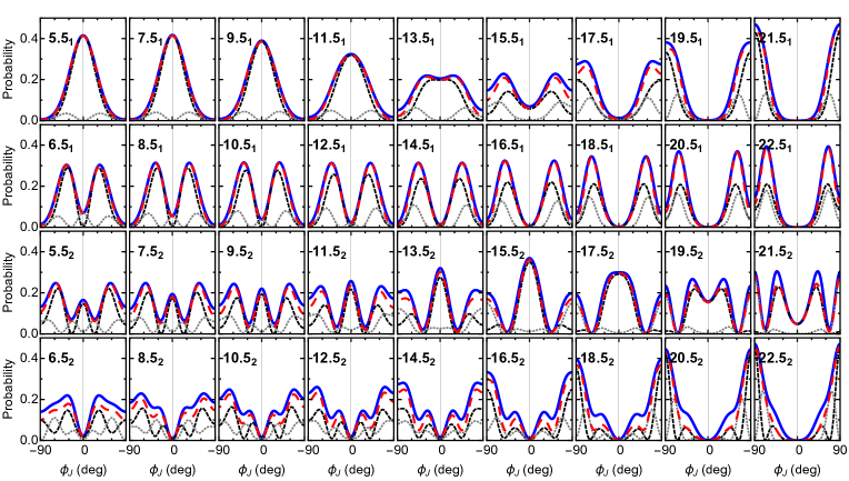
Figure 7: (Color online) Eigenstate decomposition of the SSS probability density $P(\phi_{J})$ (thick blue full curves) of the total angular momentum for the PTR $n=0$-$3$ states in ¹³⁵Pr. The individual terms are color coded as $P_{12}(\phi_{J})$ (black short dash), $P_{34}(\phi_{J})$ (gray dotted) and $P_{1234}(\phi_{J})$ (thick red long dash).

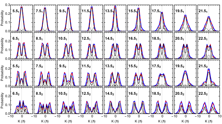
Figure 8: (Color online) Eigenstate decomposition of the probability distributions of the total angular momentum projection on the $l$ axis $P(K)$, $P_{12}(K)$, $P_{34}(K)$, and $P_{1234}(K)$ for the $n=0$-$3$ states in ¹³⁵Pr calculated by PTR. Only the region $-9.5\leq K\leq 9.5$ is shown. Same color coding as in Fig. 7.

V Entropy and coherence

V.1 Eigenvalue spectra of the reduced density matrix

As discussed above one can quantify the degree of entanglement and coherence by diagonalizing the reduced density matrix. Figure 5 displays the eigenvalues of the reduced density matrices for the PTR states of ¹³⁵Pr as functions of spin for the $n=0$, $1$, $2$, and $3$ states. For a pure, completely coherent state one eigenvalue is 1 and all other are zero. The pure triaxial rotor states are examples, which appear as the limiting case of zero Coriolis coupling in even-even nuclei. For partial coherence one has one large eigenvalue, the eigenvector of which represents the coherent wave function and the eigenvalue its probability. The remaining eigenfunctions, which appear with the probability of their small eigenvalues, distort the coherence.

As discussed above for the odd-$A$, the eigenvalues of the $\bm{j}$-density matrix are two-fold degeneracy due to Kramer’s degeneracy. The same holds for the non-zero eigenvalues of the $\bm{J}$-density matrix, which are identical. That is, the limit of complete coherence corresponds to two eigenvalues of 1/2. For partial coherence one has one large pair of eigenvalues, the eigenvector of which represents the coherent wave function and the eigenvalues their probabilities. The remaining eigenfunctions, which appear with the probabilities of their small pairs of eigenvalues, distort the coherence.

From Fig. 5, one finds that the $I=11/2,~{}n=0$ state is dominated with the probability of 0.44 by one pair of eigenvectors. For the $I=13/2,~{}n=1$ state the largest probability is 0.38, for the $I=11/2,~{}n=2$ state it is 0.34, and for the $I=13/2,~{}n=3$ state it has fallen to 0.25. The dominance of one pair decreases with the excitation energy. For the $n=1,~{}3$ sequences, the probability for the strongest eigenstate decreases smoothly with $I$. For the $n=2,~{}4$ sequences the $I$ dependence is more complex. The eigenvalues of the most likely and second likely pair of eigenvectors approach each other in the TW region, stay close in the flip region, and depart from each other in the LW region. The two pairs seem to exchange their character with increasing $I$. The eigenvalues of SP band shows similar trend as those of $n=0$ band. In Sec. V.4 we will discuss how the $I$ dependence of the eigenvectors of the $\bm{j}$- and $\bm{J}$-reduced density matrices is reflected by the structure of the PTR states.

V.2 Entropy and purity

Using the eigenvalues of the reduced density matrix, we can easily calculate the entropy $S$ and purity $\mathcal{P}$ using Eqs. (21) and (27), respectively. In Figs. 1(b) and (c), we present $S$ and $\mathcal{P}$ as functions of spin for the $n=0$, 1, 2, and $3$ states in ¹³⁵Pr calculated by the PTR. Naturally, the purity exhibits an opposite behavior compared to the entropy. A large purity corresponds to a small entropy, while a small purity corresponds to a large entropy. Therefore, in our discussions, we will focus on the behavior of the vN entropy.

For fundamental reasons, one expects that the vN entropy should increase with excitation energy, that is, the particle and total angular momenta should become more entangled with the wobbling number $n$. One could also expect that $S$ growths with the value of $I$, because the Coriolis interaction becomes stronger. Figure 1(b) demonstrates the expected behaviour is only seen in the TW region. Above, $S$ does not change much with $I$, and the states group around 0.7 with no specific order. We attribute this to the smallness of the system.

In accordance with the entropy, the purity decreases in the TW region. Above, the states group around 0.2, which is more than twice the minimal value of $1/d_{j}=1/(2j+1)=0.083$.

The entropy and purity reflect the $I$ dependence of the eigenstates of the density matrices, which were discussed in Sec. V.1. In particular the avoided crossing of two largest eigenvalues of the $n=0$ and 2 bands is seen as the exchange of the order.

Figure 1(b) includes the minimum of the entropy $S^{\textrm{(min)}}=\ln 2/\ln 12\approx 0.28$, which corresponds to the strong-coupling limit of the PTR model Ring and Schuck (1980), where the Coriolis Hamiltonian $\hat{H}_{\textrm{cor}}$ (6) is set to zero. The realistic entropy values of the $n=0$, 1, 2, and $3$ states are well above $S^{\textrm{(min)}}$, indicating that the particle angular momentum is substantially entangled with the total angular momentum.

V.3 Decoherence

The impurity causes decoherence, that is, it washes out the interference pattern of pure wave function. In order to quantify the washing out we introduced the decoherence measures (31) and (36). They compare the probability densities $P$ with the purified densities $P_{2}$ (By squaring, the small eigenvalues $p_{m}$ are suppressed relative to the large ones.)

Figure 2 compares $P(K)$ with $P_{2}(K)$. The difference between the curves indicates the missing coherence. The deviations of $P(K)$ from $P_{2}(K)$ are small, where $P_{2}(K)$ has more pronounced minima and maxima than $P(K)$. The visual impression of good partial coherence is reflected by $\Delta_{K}$ in Fig. 6, which shows the total area between the two curves in Fig. 2. The decoherence measure $\Delta_{K}$ is between 0.1 and 0.3 for all $I$. We found that $\Delta_{K}$ stays below 0.33 for all PTR states while the entropy approaches 0.80 (=1.99 in natural units) and the purity decreases to 0.15 with increasing excitation energy.

Figure 3 compares $P(\phi_{J})$ with $P_{2}(\phi_{J})$. The deviations are small as well, where $P_{2}(\phi_{J})$ has more pronounced minima and maxima than $P(\phi_{J})$. Figure 6 shows $\Delta_{\textrm{SSS}}$ which measures corresponding absolute deviation, i.e., the area between the curves. The good partial coherence corresponds to $\Delta_{\textrm{SSS}}$ stays between 0.1 and 0.3. Like $\Delta_{K}$ it stays below 0.27 for all PTR states.

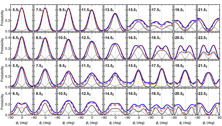
Figure 9: (Color online) Decomposition the SSS probability density distributions $P(\phi_{j})$, $P_{12}(\phi_{j})$, $P_{34}(\phi_{j})$, and $P_{1234}(\phi_{j})$ of the proton particle angular momentum for the PTR $n=0$-$3$ states in ¹³⁵Pr. Same color coding as in Fig. 7.

V.4 Nature of decoherence

According to Eqs. (17) and (18), the matrix elements of the reduced density matrix $\rho_{KK^{\prime}}$ and $\rho_{kk^{\prime}}$ can be written as the sum of the product of the eigenvalues and the normalized eigenvectors. Each term represents a pair of pure states in the $\bm{J}$- and $\bm{j}$-subspaces, which are orthonormal. The PTR states can be interpreted as the incoherent sums of the normalized probability distributions of these pairs of states in the subspaces, which are weighted by their eigenvalues.

In most cases the oscillations of the probability distributions of the respective sub-matrices reflect their mutual orthogonality. However, the SSS representations of the eigenvectors are complex. Only the different oscillations of the squares of their real parts reflect that two states are orthogonal. The same holds for their imaginary parts. If the amplitudes of the oscillations of the real and imaginary parts are similar and their zeros differently located, they may get washed out in sum, which represents the probability distribution.

Figure 5 shows that the sum of the first and second pair of eigenvalues exhausts most of the trace of the reduced density matrices, which is one. This indicates that $\rho_{KK^{\prime}}$ and $\rho_{kk^{\prime}}$ are dominated by the pairs eigenvectors of the first four eigenstates. Because of the degeneracy of the eigenvalues, we define the following coherent sub-matrices

$$\rho_{KK^{\prime}}^{(m)} =p_{m}C^{(m)}_{IK}C^{(m)}_{IK^{\prime}},$$ (41)

$$\rho_{KK^{\prime}}^{(12)} =\rho_{KK^{\prime}}^{(1)}+\rho_{KK^{\prime}}^{(2)},$$ (42)

$$\rho_{KK^{\prime}}^{(34)} =\rho_{KK^{\prime}}^{(3)}+\rho_{KK^{\prime}}^{(4)},$$ (43)

$$\rho_{KK^{\prime}}^{(1234)} =\rho_{KK^{\prime}}^{(12)}+\rho_{KK^{\prime}}^{(34)},$$ (44)

in which the upper indexes $m$ denote the order of the eigenvalues of the density matrix. Using these sub-matrices, we calculate the corresponding $\bm{J}$-SSS plots $P_{12}(\phi_{J})$, $P_{34}(\phi_{J})$, and $P_{1234}(\phi_{J})$ for the total angular momentum and corresponding $\bm{j}$-SSS plots $P_{12}(\phi_{j})$, $P_{34}(\phi_{j})$, and $P_{1234}(\phi_{j})$ for the particle angular momentum. In addition, it is clear that the non-zero eigenvalues of $\rho_{KK^{\prime}}^{(12)}$ are $p_{1}$ and $p_{2}$, while the non-zero eigenvalues of $\rho_{KK^{\prime}}^{(1234)}$ are $p_{1}$, $p_{2}$, $p_{3}$, and $p_{4}$. Correspondingly, we can calculate the vN entropy for these sub-matrices according to the definition (21)

$$S^{(12)} =-p_{1}\ln p_{1}-p_{2}\ln p_{2},$$ (45)

$$S^{(1234)} =-p_{1}\ln p_{1}-p_{2}\ln p_{2}-p_{3}\ln p_{3}-p_{4}\ln p_{4}.$$ (46)

Obviously, $S^{(1234)}$ is larger than $S^{(12)}$.

Figure 7 compares the probability $P(\phi_{J})$ of the total angular momentum with $P_{12}(\phi_{J})$, $P_{34}(K)$, and $P_{1234}(K)$, Fig. 8 compares the probability $P(K)$ of the total angular momentum with $P_{12}(K)$, $P_{34}(K)$, and $P_{1234}(\phi_{J})$, and Fig. 9 compares the SSS probability $P(\phi_{j})$ of the proton particle angular momentum with $P_{12}(\phi_{j})$, $P_{34}(\phi_{j})$, and $P_{1234}(\phi_{j})$ for the PTR $n=0$-$3$ states in ¹³⁵Pr. As seen, to good approximation the full PTR probabilities can be interpreted as the incoherent combinations of the contributions from the first two pairs of eigenvectors of the reduced density matrix.

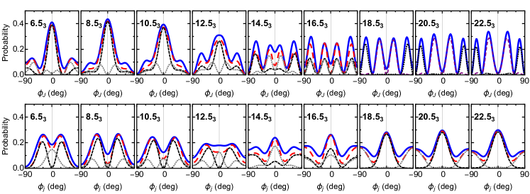
Figure 10: (Color online) Eigenstate decomposition the probability density of the total $P(\phi_{J})$, $P_{12}(\phi_{J})$, $P_{34}(\phi_{J})$, and $P_{1234}(\phi_{J})$ (upper panels) and proton particle $P(\phi_{j})$, $P_{12}(\phi_{j})$, $P_{34}(\phi_{j})$, and $P_{1234}(\phi_{j})$ (lower panels) angular momenta of the SP band in ¹³⁵Pr. In the last three panels of the upper row only $P_{12}(\phi_{J})$ and $P_{34}(\phi_{J})$ are shown. Same color coding as in Fig. 7.

The distributions $P_{12}(\phi_{J})$ and $P_{12}(K)$ are related to each other by a Fourier transform of their respective sub-density matrices. This is reflected by similar oscillation pattern. In case of harmonic oscillations they would agree when scaled by the oscillator lengths. There is a difference in the display because $K$ is a discrete variable while $\phi_{J}$ is a continuous variable. (See discussions below of the density matrices in the complete discrete $\phi_{J}$ representation.) The same Fourier-transform relation holds between $P_{34}(\phi_{J})$ and $P_{34}(K)$.

The results of $S^{(12)}$ and $S^{(1234)}$ are further included in Fig. 1(b). As seen in Fig. 1(b), $S^{(12)}$ ($=0.74$ in natural units) is very close to $S^{\textrm{(min)}}$ ($=\ln{2}=0.69$ in natural units) and $S^{(1234)}$ is restricted to a narrow band around 0.5 ($=1.2$ in natural units). This explains why the decoherence measures remain roughly constant with increasing $I$. The “noise” from the $m>4$ eigenstates does not generate much decoherence like thermal noise does not disturb the interference pattern of electromagnetic waves in a medium. In the following we discuss in detail the interpretation of the lowest four PTR states in ¹³⁵Pr.

$n=0$ states:

For the $I\leq 31/2$ yrast states the $\bm{j}$-SSS probability $P_{12}(\phi_{j})$ of the particle shows a bump at $\phi_{j}=0^{\circ}$, which indicates that the proton is in its lowest state of a potential centered at $\phi_{j}=0^{\circ}$. The width of the bump increases as the potential becomes softer with $I$. For $I=35/2$, the bump becomes unstable and is shifted to $\phi_{j}=\pm 90^{\circ}$ with further increase of $I$, which indicates that the proton is in the lowest state of a potential centered there.

The $\bm{J}$-SSS probability $P_{12}(\phi_{J})$ of the total angular momentum can be interpreted as representing the lowest states of an effective collective Hamiltonian in the $\bm{J}$-degree of freedom with a potential that changes from being being centered at $\phi_{J}=0^{\circ}$ to being centered at $\phi_{J}=\pm 90^{\circ}$.

The SSS $\bm{j}$-probability $P_{34}(\phi_{j})$ has the double hump structure of the second state of the particle in a potential that changes around $I=31/2$ from being centered at $\phi_{j}=0^{\circ}$ to being centered at $\phi_{j}=\pm 90^{\circ}$. For $I<31/2$ the distribution $P_{34}(\phi_{j})$ has a zero at $\phi_{j}=0^{\circ}$, while for $I>31/2$ it has zeroes at $\phi_{j}=\pm 90^{\circ}$. Around $I=31/2$ there are only minima at $\phi_{j}=0^{\circ},~{}\pm 90^{\circ}$ corresponding to the transitional character of the potential.

The SSS $\bm{J}$-probability $P_{34}(\phi_{J})$ has the double hump structure of the second state of the total angular momentum in the effective collective potential. It corrects the $P_{12}(\phi_{J})$ term by widening the peaks, flattening their apexes and enhancing the dips at $\phi_{J}=0^{\circ}$ in the flip region.

$n=1$ states:

For $I\leq 29/2$ the $\bm{j}$-SSS probability $P_{12}(\phi_{j})$ of the particle is similar to the one of the $n=0$ state. The bump at $\phi_{j}=0^{\circ}$ indicates that the proton is in its lowest state of a potential centered there. The width of the bump increases as the potential becomes softer with $I$. At larger $I$ values a dip at $\phi_{j}=0^{\circ}$ develops, while the zeroes at $\phi_{j}=\pm 90^{\circ}$ remain. The SSS $\bm{j}$-distribution $P_{34}(\phi_{j})$ has a double hump structure that is similar to the $n=0$ state.

The $\bm{J}$-SSS probability $P_{12}(\phi_{J})$ of the total angular momentum represents to good approximation the second states of the collective Hamiltonian in the $\bm{J}$-degree of freedom with a potential that changes from being centered at $\phi_{J}=0^{\circ}$ to being centered at $\phi_{J}=\pm 90^{\circ}$.

The SSS $\bm{J}$-distribution $P_{34}(\phi_{J})$ changes with $I$ from an $n=3$ like triple-peak structure in a potential centered at $\phi_{J}=0^{\circ}$ to the two separated peaks at large $I$, which are similar to the ones of the $n=0$ states in the panel above. The orthogonality of the states 1, 2, 3, 4 becomes only apparent when one plots the densities of their real and imaginary parts separately.

$n=2$ states:

The $\bm{j}$-SSS distributions $P_{12}(\phi_{j})$ have a peak at $\phi_{j}=0^{\circ}$ similar to the $n=0,1$ states in the TW wobbling regime. At variance with them, the peak stays about the same up to the largest $I$ values. The reaction to the Coriolis force appears as the change of the $P_{34}(\phi_{j})$ distribution from two peaks located near $\phi_{j}=\pm 45^{\circ}$ to two peaks at $\phi_{j}=\pm 90^{\circ}$ while the value at $\phi_{j}=0^{\circ}$ remains always zero.

The $\bm{J}$-SSS distributions $P_{12}(\phi_{J})$ determine the character of the total distribution. In the TW wobbling region $I\leq 23/2$ it has three peaks at $\phi_{J}=0^{\circ},\approx\pm 45^{\circ}$, which reflect the typical nodal structure of a collective state in a potential centered at $\phi_{J}=0^{\circ}$. The $P_{34}(\phi_{J})$ term leads to some modification, which is similar to the corrections to the $n=0,1$ states. At larger $I$ values, the $P_{12}(\phi_{J})$ distribution changes into a LW-like $n=2$ structure with peaks at $\phi_{J}=\pm 90^{\circ},~{}\approx\pm 45^{\circ}$. The total function $P$ is similar because $P_{34}$ is small.

$n=3$ states:

For $I=17/2,~{}21/2$ the $\bm{j}$-SSS distributions $P_{12}(\phi_{j})$ have peak at $\phi_{j}=0^{\circ}$. Like the PTR states $n=0,~{}1,~{}2$, the $P_{34}(\phi_{j})$ distributions have two peaks, but with lager weight. The sum $P_{1234}(\phi_{j})$ gives a broader $\phi_{j}=0^{\circ}$ peak. The $\bm{J}$-SSS distributions $P_{12}(\phi_{J})$ have the typical $n=3$ nodal structure with zeros at $\phi_{J}=0^{\circ},\approx\pm 35^{\circ}$ and maxima at $\phi_{J}\approx\pm 25^{\circ},~{}\approx\pm 65^{\circ}$. The relatively large incoherent contribution $P_{34}(\phi_{J})$ considerably washes out the oscillation of the total distribution.

At larger $I$, the $\bm{j}$-SSS distributions $P_{12}(\phi_{j})$ and $P_{34}(\phi_{j})$ contribute with similar weight. The distributions $P(\phi_{j})$ develop an increasing minimum at $\phi_{j}=0^{\circ}$, which indicates the gradual alignment of the particle with the $m$-axis. The $\bm{J}$-SSS distributions $P_{12}(\phi_{J})$ and $P_{34}(\phi_{J})$ contribute with similar weight as well. As the result of their incoherent combination, $P(\phi_{J})$ becomes localized at $\phi_{J}=\pm 90^{\circ}$ for $I=45/2$.

SP states:

Figure 10 compares $P(\phi)$ with the $P_{12}(\phi)$, $P_{34}(\phi)$, and $P_{1234}(\phi)$ for the total and proton particle angular momenta of SP band in ¹³⁵Pr, which is built on the state $13/2_{3}$ (see Fig. 1). As common, the name “SP” is used to denote the first excited state of the odd proton in the rotating potential. The excitation corresponds to a certain reorientation of $\bm{j}$ away from the $s$ axis, which is reflected by the appearance of two peaks symmetric $\phi_{j}=0^{\circ}$ in the $\bm{j}$-probability density $P(\phi_{j})$ when $I\leq 23/2$. For these $I$ values the $\bm{J}$-probability $P(\phi_{J})$ has a pronounced peak at $\phi_{J}=0^{\circ}$, which indicates that the nucleus is uniformly rotating about the $s$ axis.

As seen in Fig. 1, the states $13/2_{2}$ and $13/2_{3}$ are close to each other. We discussed in our previous study Chen and Frauendorf (2022) that the two states represent a mixture of a pure $n=2$ TW state and a pure SP state. The mixture is clearly seen as the dip in the $\bm{j}$-distribution of the $13/2_{2}$ state.

For $I\geq 25/2$, the $\bm{j}$-distributions develop a peak at $\phi_{j}=0^{\circ}$ similar to the $n=2$ states $(I-1)_{2}$. Along with this, a minimum at $\phi_{j}=0^{\circ}$ appears in the $n=3$ distributions, which indicates the reorientation of $\bm{j}$ towards the $m$ axis.

For $I\geq 25/2$, the $\bm{J}$-distribution changes to an oscillation with zeroes at $\phi_{J}=0^{\circ}$, $\pm 60^{\circ}$, $\pm 90^{\circ}$, which corresponds to a $n=3$ wobbling mode without much modification by the odd particle. As already discussed in (d), the $\bm{J}$-distributions of the $n=3$ states change to rotation about the $m$ axis. It seems that the SP band and the $n=3$ band interchange their character over the $I\geq 25/2$ region.

V.5 Two-quasiparticle bands

The TW mode based on the $(1h_{11/2})^{2}$ two-quasiproton in ¹³⁰Ba has been studied in Ref. Chen et al. (2019) in the framework of the PTR model, where the details are given. As described in the Sec. II.1, the reduced two-quasiparticle density matrix is obtained by Eq. (14), where the index $k_{12}=k_{1}+k_{2}$ and the sum runs over all projections $K$ and all couplings of the two quasipartilcles to $\bm{j}_{12}$. The reduced density matrix for the total angular moment is obtained by Eq. (16), where the sum runs over all projections $k_{1}$ and $k_{2}$ of the two quasiparticles.

Figure 11: Eigenvalues of the reduced density matrices of ¹³⁰Ba as functions of spin for the $n=0$, $1$, $2$, and $3$ states. The slant shadow denotes the eigenvalues below 0.2. In contrast to the case of ¹³⁵Pr in Fig. 5, the paired eigenvalues $(p_{1},p_{2})$, $(p_{3},p_{4})$, …. are not the same. However, the differences are within the size of the symbols.

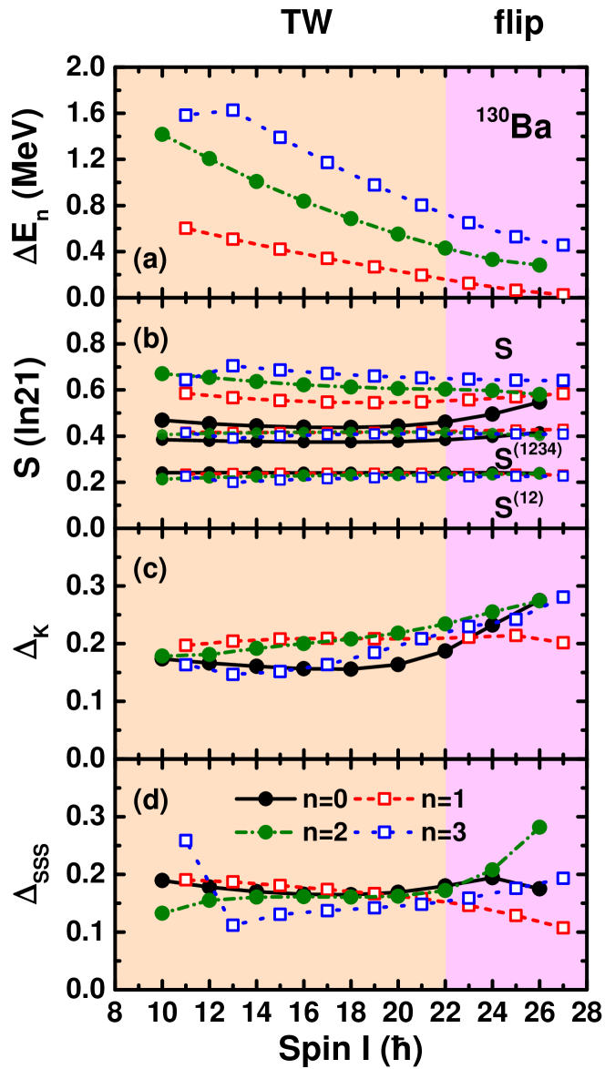
Figure 12: (Color online) (a) Excitation energies of the wobbling bands in ¹³⁰Ba with wobbling numbers $n=1$, 2, and 3 with respect to the zero wobbling energy $\bar{E}_{\textrm{yrast}}(I)$ calculated by the PTR. (b) The entropy $S$, $S^{(1234)}$, and $S^{(12)}$ of the states in unit of $\ln 21$, where 21 is the dimension of the two-qp $\pi(h_{11/2})^{2}$ space. (c) The absolute deviations $\Delta_{K}$ of the $K$ distributions $P(K)$. (d) The absolute deviations $\Delta_{\textrm{SSS}}$ of the SSS plots $P(\phi_{J})$. The different backgrounds delineate the regions of the TW and flip modes.

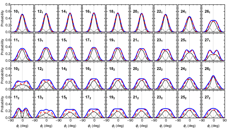
Figure 13: (Color online) Eigenstate decomposition of the SSS probability density $P(\phi_{j})$, $P_{12}(\phi_{j})$, $P_{34}(\phi_{j})$, and $P_{1234}(\phi_{j})$ of the two-proton angular momentum for the PTR states $n=0$-$3$ states in ¹³⁰Ba. Same color coding as in Fig. 7.

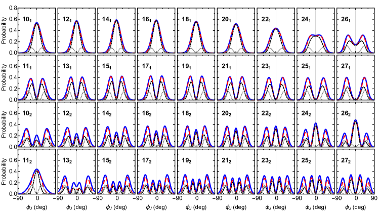
Figure 14: (Color online) Eigenstate decomposition of the SSS probability density $P(\phi_{J})$, $P_{12}(\phi_{J})$, $P_{34}(\phi_{J})$, and $P_{1234}(\phi_{J})$ of the total angular momentum for the PTR $n=0$-$3$ states in ¹³⁰Ba. Same color coding as in Fig. 7.

Figure 11 displays the eigenvalues of the reduced density matrix as functions of spin for the $n=0$, $1$, $2$, and $3$ states in ¹³⁰Ba. Unlike the case of ¹³⁵Pr, there are no degenerate pairs $p_{1}=p_{2}$, $p_{3}=p_{4}$, $...$ of the eigenvalues of the reduced density matrices in ¹³⁰Ba because the dimensions of even-$K$ and odd-$K$ bases are different. However, the spectra consist of pairs of very close eigenvalues $p_{1}\approx p_{2}$, $p_{3}\approx p_{4}$, $...$, which are not distinguishable in the figure. Like in the case of ¹³⁵Pr, the first two pairs of eigenvalues dominate the spectrum for all $n=0$, 1, 2, and 3 states.

Figure 12 shows the excitation energies $\Delta E_{n}(I)$, the vN entropy $S$, $S^{(12)}$, and $S^{(1234)}$, as well as the decoherence measures $\Delta_{K}$ and $\Delta_{\textrm{SSS}}$ of the wobbling bands in ¹³⁰Ba with wobbling numbers $n=0$, 1, 2, and 3. As discussed in our previous work Chen and Frauendorf (2024), the TW regime in ¹³⁰Ba extends to $I=22$, beyond which the regime transitions into the flip regime. Accordingly, the energy spectrum evolves from the equidistant harmonic TW pattern at low $I$ values to $\Delta E_{n=1}(I)\approx 0$ at $I=26$, signifying the onset of TW instability.

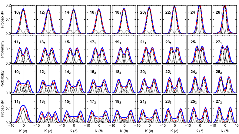
Figure 15: (Color online) Decomposition the probability distribution of the total angular momentum projection on the $l$ axis $P(K)$, $P_{12}(K)$, $P_{34}(K)$, and $P_{1234}(K)$ for the $n=0$-$3$ states of ¹³⁰Ba calculated by PTR. Only the region $-10\leq K\leq 10$ is shown. Same color coding as in Fig. 7.

The vN entropy $S^{(12)}$ of the four PTR states is about 0.25 ($=0.74$ in natural units), which is very close to the value of ¹³⁵Pr. The vN entropy $S^{(1234)}$ is confined to a narrow band around 0.4 ($=1.2$ in natural units) which agrees with the band in ¹³⁵Pr. We attribute the agreement to same number of eigenstates (2 and 4, respectively) taken into account in the sub-matrices. Compared with the TW region in ¹³⁵Pr, the full vN entropy $S$ shows more clearly the expected increasing order with $n$, which reflects the larger number of states in two-quasiparticle basis than in the one-quasiparticle basis (12 vs. 21, respectively). Like in ¹³⁵Pr, the four states come together near 0.6 with increasing $I$, and their trend indicates that the order becomes scrambled.

The function $S(I)$ reflects the $I$ dependence of the eigenvalues $p_{m}$ in Fig. 11. The approach of $(p_{1},p_{2})$ and $(p_{3},p_{4})$ at large $I$ for the $n=0$ state is seen as the increase of the entropy in Fig. 12(b). For the $n=1$ state the distancing of $(p_{1},p_{2})$ from $(p_{3},p_{4})$ is seen as the decrease of the entropy. For the $n=3$ state, there is an abrupt decrease of $(p_{1},p_{2})$ from $I=11$ to $I=13$. This is attributed to the fact that the $11_{2}$ state has a SP structure, while the $13_{2}$ state has $n=3$ character. The structural change is reflected by the entropy increase in Fig. 12(b).

In analogy to ¹³⁵Pr, the incoherence measures $\Delta_{K}$ and $\Delta_{\textrm{SSS}}$ fall into a interval between about 0.15 and 0.35, and do not show a systematic $I$ and $n$ dependence. These values suggest that the density matrix exhibits partial coherence.

Figures  13 and  14 show, respectively, the eigenstate decomposition of the $\bm{j}$-SSS $P(\phi_{j})$ and $\bm{J}$-SSS $P(\phi_{J})$ distributions for the states in ¹³⁰Ba. Similar to ¹³⁵Pr, the function $P_{1234}(\phi_{J})$ well approximates the total distribution $P(\phi_{J})$.

Figure 13 shows that, as for ¹³⁵Pr, the probability densities $P_{12}(\phi_{j})$ have a peak at $\phi_{j}=0^{\circ}$, indicating the alignment of the proton pair with the $s$ axis, and $P_{34}(\phi_{j})$ are the double-peak distributions, which account for the realignment of the proton pair. The contribution of $P_{34}(\phi_{j})$ becomes more important with the wobbling number $n$. The “noise” from the $m>4$ eigenstates washes out the structure of $P_{1234}(\phi_{j})$ to some extent.

The SP structure of the PTR state $11_{2}$ is recognized as the double hump of the leading term $P_{12}(\phi_{j})$ and the triple hump of $P_{34}(\phi_{j})$ (compare with Fig. 10, states $8.5_{3}$, $10.5_{3}$, $12.5_{3}$). The function $P(\phi_{J})$ in Fig. 14 has one peak at $\phi_{J}=0^{\circ}$ that is characteristic for the signature partner state.

As illustrated in Fig. 14, the $\bm{J}$-SSS probability $P(\phi_{J})$ for yrast states of the total angular momentum exhibits a pronounced peak at $\phi_{J}=0^{\circ}$ for $I\leq 22$. This peak suggests that the total angular momentum is predominantly in the lowest potential state aligned with $\phi_{J}=0^{\circ}$ (c.f. Fig. 10 of Ref. Chen and Frauendorf (2024)). As the spin $I$ increases, the potential becomes increasingly softer, resulting in a broadening of this peak. For $I=24$, this peak becomes unstable and shifts towards $\phi_{J}=\pm 90^{\circ}$, signifying the onset of a TW instability.

The functions $P(\phi_{J})$ for the remaining PTR states show oscillation that are typical for $n=1$, 2, and 3 states in a potential with a center that shift from $\phi_{J}=0$ to $\pm 90^{\circ}$. The corresponding shift of maximal amplitude from $\phi_{J}=0$ to $\pm 90^{\circ}$ is the reason why in Fig. 13 for the $n=2$ and 3 states $P_{12}(\phi_{j})$ is comparable with $P_{34}(\phi_{j})$ at low $I$ while $P_{12}(\phi_{j})$ is dominates $P_{34}(\phi_{j})$ at large $I$. This, at first thought, unexpected trend reflects that $\bm{j}$ adiabatically follows $\bm{J}$ (see next section).

Furthermore, Fig. 15 show the decomposition of the $P(K)$ distributions for the PTR $n=0$-$3$ states in ¹³⁰Ba. The function $P_{1234}(K)$ well reproduces the total distribution $P(K)$. With increasing $n$ or $I$, $P_{34}(K)$ plays more and more important role.

VI Entanglement and adiabatic approximation

In Ref. Chen and Frauendorf (2024), we derived a collective Hamiltonian (CH) for the $\bm{J}$-degree of freedom by applying the classical adiabatic approximation to the $\bm{j}$-degree of freedom. This detour via a classical Hamiltonian and its re-quantization results in a collective wave function with a pure density matrix. In this section we discuss the relation with the concept of coherence based on the eigenstate decomposition. The adiabatic approximation relies on the a fast time scale for $\bm{j}$ compared to a slow time scale for $\bm{J}$. That is, the lower the wobbling excitations the better the description by the CH.

The reduced density matrix $\rho_{\phi_{J},\phi_{J}^{\prime}}$ is approximated by a pure density matrix $\rho_{\phi_{J},\phi_{J}^{\prime}}^{(\textrm{CH})}$ generated from the collective eigenfunction of the effective CH in the $\bm{J}$-degree of freedom. The coupling to the $\bm{j}$-degree of freedom is taken into account assuming that $\bm{j}$ follows $\bm{J}$ in an adiabatic way, which is an alternative to describing the entanglement of the two degrees of freedom by means of the Schmidt decomposition. In detail, this means that the total angular momentum operator $\bm{\hat{J}}$ in the PTR Hamiltonian (1) is replaced by the c-number $\bm{J}$. The adiabatic energy $E(\bm{J})$ is calculated by either diagonalizing the parametric PTR Hamitonian $H_{\textrm{PTR}}(\bm{J},\bm{\hat{j}})$ and select the lowest eigenvalue (tilted axis cranking) or simply take the minimum with respect to $\bm{j}$ for fixed $\bm{J}$ of the classical energy $E(\bm{J},\bm{j})$. The adiabatic energy $E(\phi_{J},J_{3})$ has the form of a narrow valley along $J_{3}=0$, which is approximated by

$$E(\phi_{J},J_{3})=\frac{J_{3}^{2}}{2B(\phi_{J})}+V(\phi_{J})$$ (47)

in deriving the CH by re-quantization $E(\phi_{J},J_{3})\rightarrow H_{\textrm{CH}}(\phi_{J},\hat{J}_{3})$.

Figures 5 and 6 of Ref. Chen and Frauendorf (2024) compare the approximate CH energies and $E2$ transition probabilities for ¹³⁵Pr with the the PTR values. Figures 11 and 12 of Ref. Chen and Frauendorf (2024) and Fig. 21 provide the same comparison for ¹³⁰Ba. Generally, the CH approximation works quite well for ¹³⁰Ba for all $n=0$, 1, 2, and 3 states into the flip region. For ¹³⁵Pr it gives a fair description for the $n=0$, 1, and 2 states below the flip region.

VI.1 Comparison of the probability densities

The CH approximates the PTR states by a wave function in the $\bm{J}$-degree of freedom, which corresponds to a pure density matrix. In order to assess the quality, we compare the pertaining probability distribution $P_{\textrm{CH}}$ with the full distribution $P$ and the distribution calculated from the pure sub-density matrix with the largest probability $P_{12}/(p_{1}+p_{2})$. According to the Schmidt decomposition, the latter is the “best” representation as a product wave function in the $\bm{J}$ and $\bm{j}$ degrees of freedom.

As the CH couples only matrix elements $\Delta K=0$ and $\pm 2$, the eigenstates appear in pairs. In the case of odd-$A$ nucleus, the two eigenstates have $K=I-\textrm{even}$ or $K=I-1-\textrm{even}$ and the two eigenvalues are the same. In the case of even-$A$ nucleus, the two eigenstates have even-$K$ or odd-$K$ and the two eigenvalues are nearly the same. In the following figures we display the mean value of the two probability distributions $P_{\textrm{CH}}=\left(P_{\textrm{CH}}^{(1)}+P_{\textrm{CH}}^{(2)}\right)/2$.

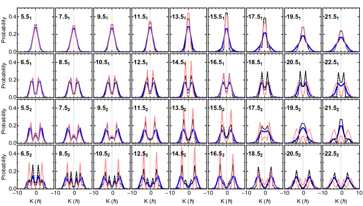
Figure 16: (Color online) Probability distribution of the total angular momentum projection on the $l$ axis $P(K)$ (thick blue full curves) and normalized $P_{12}(K)/(p_{1}+p_{2})$ (black short dashed) obtained by PTR in comparison with the $P_{\textrm{CH}}(K)$ obtained from the collective Hamiltonian (thin pink dotted) Chen and Frauendorf (2024) for the PTR states of ¹³⁵Pr. Only the region $-9.5\leq K\leq 9.5$ is shown.

Figure 16 compares the full distribution $P(K)$ and the normalized distribution $P_{12}(K)/(p_{1}+p_{2})$ with the probability $P_{\textrm{CH}}(K)$ obtained from the adiabatic CH for the $n=0$, 1, 2, and 3 states of ¹³⁵Pr. As seen, $P_{\textrm{CH}}(K)$ agrees well with $P_{12}(K)$ for the $n=0$ states in the first row. For the $n=1$ states $13/2_{1}$-$33/2_{1}$ it also agrees reasonably well with $P_{12}(K)/(p_{1}+p_{2})$ being somewhat too spiky in the flip region. For the states $37/2_{1}$-$45/2_{1}$ the distribution $P_{\textrm{CH}}(K)$ differs from $P(K)$ and $P_{12}(K)/(p_{1}+p_{2})$. Also for the $n=2$ states $11/2_{2}$-$31/2_{2}$ the distribution $P_{\textrm{CH}}(K)$ reasonably well reproduces $P_{12}(K)/(p_{1}+p_{2})$ being somewhat too spiky in the flip region. It differs from $P(K)$ and $P_{12}(K)/(p_{1}+p_{2})$ for the states $35/2_{2}$-$43/2_{2}$. The state $13/2_{2}$ has SP character and cannot be described by the CH. For the states $17/2_{2}$-$25/2_{2}$ the distribution $P_{\textrm{CH}}(K)$ roughly traces $P_{12}(K)/(p_{1}+p_{2})$, which has $n=3$ character. The adiabatic approximation fails for larger $I_{2}$.

Figure 17 compares the full distribution $P(\phi_{J})$ and the normalized distribution $P_{12}(\phi_{J})/(p_{1}+p_{2})$ with the SSS probability $P_{\textrm{CH}}(\phi_{J})$ obtained from the adiabatic CH for the $n=0$, 1, 2, and 3 states of ¹³⁵Pr.

As seen in Fig. 17, $P_{\textrm{CH}}(\phi_{J})$ of the $n=0$ states $11/2_{1}$ and $15/2_{1}$ agrees very well with $P_{12}(\phi_{J})$, from which it deviates increasing $I$ such that it approaches $P(\phi_{J})$ for the flip state $27/2_{1}$. For the state $31/2_{1}$ above the flip region $P_{\textrm{CH}}(\phi_{J})$ deviates from $P(\phi_{J})$ such that it approaches $P_{12}(\phi_{J})$ with increasing $I$.

The wobbling energy $\Delta E_{1}$ is minimal for $I=27/2$, that is, the adiabatic approximation works best. The function $P_{\textrm{CH}}(\phi_{J})$ exhibits a more pronounced dip at $\phi_{J}=0^{\circ}$ than $P(\phi_{J})$. The reason for the difference is the following. The adiabatic classical potential accounts for the response the particle to the Coriolis force for each orientation of the total angular momentum $\bm{J}$. The term $\rho_{KK^{\prime}}^{(12)}$ is selected such that the $\bm{j}$- and $\bm{J}$-degrees of freedom are decoupled as best as possible, which corresponds to a state of the particle with an average orientation $\bm{j}=(\sqrt{\langle\hat{j}^{2}_{1}\rangle},\sqrt{\langle\hat{j}^{2}_{2}\rangle},\sqrt{\langle\hat{j}^{2}_{3}\rangle})$.

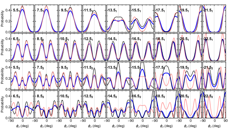
Figure 17: (Color online) The SSS probability density $P(\phi_{J})$ (thick blue full curves) and normalized SSS $P_{12}(\phi_{J})/(p_{1}+p_{2})$ (black short dashed) of the total angular momenta in comparison with the SSS probability density $P_{\textrm{CH}}(\phi_{J})$ obtained from the collective Hamiltonian (thin pink dotted) Chen and Frauendorf (2024) for the PTR states of ¹³⁵Pr.

For the $n=1$ states in the second row of Fig. 17 one observes a similar $I$ dependence. For the state $13/2_{1}$ the function $P_{\textrm{CH}}(\phi_{J})$ agrees with $P_{12}(\phi_{J})$. With increasing $I$ it changes to the full $P(\phi_{J})$ for the flip state $29/2_{1}$. Above the flip region $P_{\textrm{CH}}(\phi_{J})$ progressively deviates from both $P_{12}(\phi_{J})$ and $P(\phi_{J})$, which indicates that the adiabatic approximation becomes problematic.

The $n=2$ states in the third row of Fig. 17 show the same $I$ dependence of $P_{\textrm{CH}}(\phi_{J})$ from $P_{12}(\phi_{J})$ for $11/2_{2}$ to $P(\phi_{J})$ for $27/2_{2}$. Above the flip region $P_{\textrm{CH}}(\phi_{J})$ strongly deviates from both $P_{12}(\phi_{J})$ and $P(\phi_{J})$, which indicates that the adiabatic approximation fails. As discussed above, the incoherent term $P_{34}(\phi_{J})$ increases with the wobbling number $n$ and so the difference between $P_{\textrm{CH}}(\phi_{J})$ and $P(\phi_{J})$ at low spin.

For the states $17/2_{2}$, $21/2_{2}$, $25/2_{2}$, and $29/2_{2}$ in the lowest row of Fig. 17, $P(\phi_{J})$ has a washed-out shape of $P_{\textrm{CH}}(\phi_{J})$, which is expected because the incoherent terms $P_{34}(\phi_{J})$ are the largest. As discussed, the state $13/2_{2}$ has SP structure. The CH generates a collective $n=3$-type state with the characteristic four maxima. The adiabatic approximation fails for $I>29/2$.

In general, the distributions $P_{\textrm{CH}}(K)$ are more spiky than $P_{12}(K)/(p_{1}+p_{2})$ while the distributions $P_{\textrm{CH}}(\phi_{J})$ are smoother than $P_{12}(\phi_{J})/(p_{1}+p_{2})$, which reflects their relation by a Fourier transform.

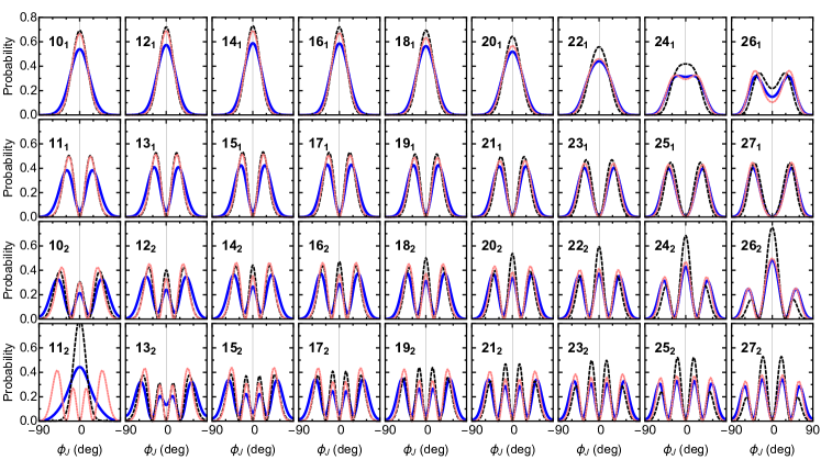
Figure 18: (Color online) The SSS probability density $P(\phi_{J})$ (thick blue full curves) and normalized SSS $P_{12}(\phi_{J})/(p_{1}+p_{2})$ (black short dashed) of the total angular momenta in comparison with the SSS probability density $P_{\textrm{CH}}(\phi_{J})$ obtained from the collective Hamiltonian (thin pink dotted) Chen and Frauendorf (2024) for the PTR states in ¹³⁰Ba.

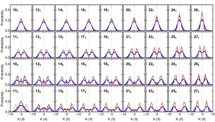
Figure 19: (Color online) Probability distribution of the total angular momentum projection on the $l$ axis $P(K)$ (thick blue full curves) and normalized $P_{12}(K)/(p_{1}+p_{2})$ (black short dashed) obtained by PTR in comparison with the $P_{\textrm{CH}}(K)$ obtained from the collective Hamiltonian (thin pink dotted) Chen and Frauendorf (2024) for the PTR states of ¹³⁰Ba. Only the region $-10\leq K\leq 10$ is shown.

For ¹³⁰Ba the functions $P_{\textrm{CH}}(\phi_{J})$ in Fig. 18 characterize the mode, as $n=0$, 1, 2, and 3 TW excitations, where $n$ counts the respective number of zeroes. As illustrated in Fig. 10 of Ref. Chen and Frauendorf (2024), the adiabatic potential of the CH is approximately quadratic around $\phi_{J}=0^{\circ}$ at low $I$ and develops a flat bottom with increasing $I$. The peak heights of $P_{\textrm{CH}}(\phi_{J})$ reflect the change of the adiabatic potential. In the harmonic TW region the maxima’s height increase with $|\phi|$ like for the corresponding Hermite polynomials. For $I=24,~{}25$ the flip region is reached. The pattern changes to equal heights with the tendency of higher peaks near $\phi_{J}=0^{\circ}$, which suggest the transition to the LW regime.

Figure 18 compares the full distribution $P(\phi_{J})$ and the normalized distribution $P_{12}(\phi_{J})/(p_{1}+p_{2})$ with the SSS probability $P_{\textrm{CH}}(\phi_{J})$ obtained from the adiabatic CH for ¹³⁰Ba. Except the SP state $11_{2}$, which has a SP structure, the $P_{\textrm{CH}}(\phi_{J})$ agree rather well with the scaled $\bm{J}$-SSS distributions $P_{12}(\phi_{J})/(p_{1}+p_{2})$ for low $I$. Analog to one-quasiparticle cases in ¹³⁵Pr, for $I>17$ the functions $P_{\textrm{CH}}(\phi_{J})$ notably deviate from the scaled probability densities $P_{12}(\phi_{J})/(p_{1}+p_{2})$ and approach the full density $P(\phi_{J})$ in the flip region, where the adiabatic approximation works best.

As discussed in the Appendix B, the $E2$ transition probabilities calculation can be approximated by replacing the trace of the product of an intrinsic quadrupole operator with the density matrix by the integral over the product of the classical quadrupole moments (53) with the probability densities $P(\phi_{J})$, $P_{12}(\phi_{J})/(p_{1}+p_{2})$, and $P_{\textrm{CH}}(\phi_{J})$. This explains why the CH transition probabilities in Fig. 21 change in the same way with $I$ as $P_{\textrm{CH}}(\phi_{J})$. At low $I$, where the adiabatic approximation is less accurate, they agree with the values by $P_{12}(\phi_{J})/(p_{1}+p_{2})$ and for large $I$, where the adiabatic approximation is more accurate, they agree with the PTR values by $P(\phi_{J})$.

Figure 19 compares the full distribution $P(K)$ and the normalized distribution $P_{12}(K)/(p_{1}+p_{2})$ with the probability $P_{\textrm{CH}}(K)$ obtained from the adiabatic CH for ¹³⁰Ba. Similar to ¹³⁵Pr, $P_{\textrm{CH}}(K)$ agrees well with $P_{12}(K)/(p_{1}+p_{2})$ for all $I$. The features of wobbling excitations with $n=0$, 1, 2, and 3 are reflected by the number of the nodes in the $P_{\textrm{CH}}(K)$ plots. Only for $11_{2}$ state, which has a SP structure, $P_{\textrm{CH}}(K)$ fails to reproduce $P_{12}(K)/(p_{1}+p_{2})$. The $E2$ matrix elements do not depend on the basis they are calculated from. This is not at variance with the fact that $P_{\textrm{CH}}(K)$ agrees with $P_{12}(K)/(p_{1}+p_{2})$ for all $I$ while $P_{\textrm{CH}}(\phi_{J})$ deviates from it. The non-diagonal matrix elements of the operator $\hat{Q}_{\pm 2}$ generate the differences in a non-obvious way (see details in the Appendix A).

The quadratic approximation (47) of the adiabatic energy explains the different $I$ dependence of $P_{\textrm{CH}}$ in comparison with $P$ and $P_{12}$ in Figs. 18 and 19. It maps out the potential $V(\phi_{J})$ in detail while the kinetic term is approximated to be quadratic in $\hat{J}_{3}$. The CH provides low-lying wave functions in the $\phi_{J}$-degree of freedom that are the better the smaller their kinetic energy is. As a consequence, $P_{\textrm{CH}}(\phi_{J})$ approaches $P(\phi_{J})$. This is not the case for the kinetic term which does not fully map out $E(\phi_{J},J_{3})$ in $J_{3}$ direction. Moreover, the SSS basis states are maximal localized in $\phi_{J}$ and maximal uncertain in $K$ (constant weight).

VI.2 Comparison of the density matrices

In calculating the reduced density matrix, the tracing out of the $\bm{j}$-degree of freedom destroys to some extend the coherence of the complete PTR wave function. The properties of the $\bm{J}$-degrees of freedom are described by the reduced density matrix, which cannot be further simplified. As we discussed in the previous section, it represents an ensemble of quantal states in the $\bm{J}$-subspace with the probability $p_{m}$. These states are entangled with pertaining quantal states $\bm{j}$-subspace, which appear with the same probability $p_{m}$. That is, the combined system can be interpreted as an ensemble, where $\bm{J}$ and $\bm{j}$ appear in pairs of quantal states in the respective subspaces.

The description of the PTR system in terms of the effective CH accounts for the entanglement by means of the approximation that $\bm{j}$ adiabatically follows $\bm{J}$, which implies coherence. Accordingly the pure density matrix $\rho^{\textrm{(CH)}}$ represents the coupled system. In the Appendix A, we compare $\rho^{(\textrm{CH})}$ with the mixed matrix $\rho$ and the pure sub-matrix $\rho^{(12)}$ for the PTR states $10_{1}$ and $26_{2}$ in ¹³⁰Ba in order to illustrate their relations.

The density matrices $\rho_{KK^{\prime}}$ and $\rho_{\phi_{J},\phi_{J}^{\prime}}$ are related to each other by the Fourier transform between the $K$ and $\phi_{J}$ representations. However, their diagonal matrix elements are not related by a simple Fourier transform, because the basis change involves the non-diagonal matrix elements as well. As discussed, the diagonal matrix elements $\rho^{(\textrm{CH})}_{KK}$ approximate $\rho^{(12)}_{KK}/(p_{1}+p_{2})$ of the pure sub-density with the largest weight in $\rho_{KK^{\prime}}$, which loosely speaking realizes as good as possible one factor of the product wave function (with $\rho^{(12)}_{kk^{\prime}}/(p_{1}+p_{2})$ being the other factor). When the diagonal matrix elements of $\rho^{(\textrm{CH})}_{\phi_{J},\phi_{J}^{\prime}}$ approach the diagonal matrix elements of $\rho_{\phi_{J},\phi_{J}^{\prime}}$, the non-diagonal matrix elements of the two matrices remain different. However, these matrix elements are insignificant in calculating the $E2$ transition matrix elements as discussed in the Appendix B. An analog consideration applies to the $M1$ operator, which involves the adiabatic response of $\bm{j}$ explicitly. Hence, the concept of a coherent wave function is appropriate as long as this kind of quasi-local in $\phi_{J}$ operators are of interest. Operators that involve highly non-diagonal matrix elements are not amenable to the adiabatic approximation.

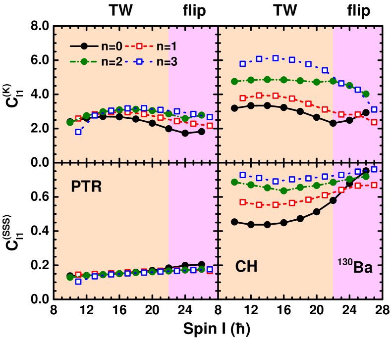
Figure 20: (Color online) Calculated $C_{l_{1}}^{(K)}$ and $C_{l_{1}}^{(\textrm{SSS})}$ of the density matrices $\rho_{KK^{\prime}}$ and $\rho_{\phi_{m},\phi_{n}}$ as functions of spin by PTR and CH for the $n=0$-$3$ states in ¹³⁰Ba.

To characterize the coherence properties of the density matrices of PTR and CH, Fig. 20 further displays the $l_{1}$ norm $C_{l_{1}}$ of density matrices $\rho_{KK^{\prime}}$ and $\rho_{\phi_{m},\phi_{n}}$ as functions of spin $I$ for $n=0$-$3$ calculated from the PTR and CH states in ¹³⁰Ba. In general, the $C_{l_{1}}$ of CH is larger than that of PTR, indicating that a larger number of non-diagonal matrix elements is needed to generate the pure density matrix of a coherent eigenstae of the CH. The $C_{l_{1}}$ norm increases with adding wobbling quanta $n$ to the CH eigenstates, while $C_{l_{1}}$ of the PTR states does not change much.

VI.3 Comparison of electromagnetic properties

The $E2$ transition probabilities are obtained by tracing the product of an intrinsic quadrupole operator (B) with the density matrix. The examples of density matrix and quadrupole matrix elements are given in the Appendixes A and B, respectively, for $10_{1}$ and $26_{2}$ states of ${}^{130}\textrm{Ba}$.

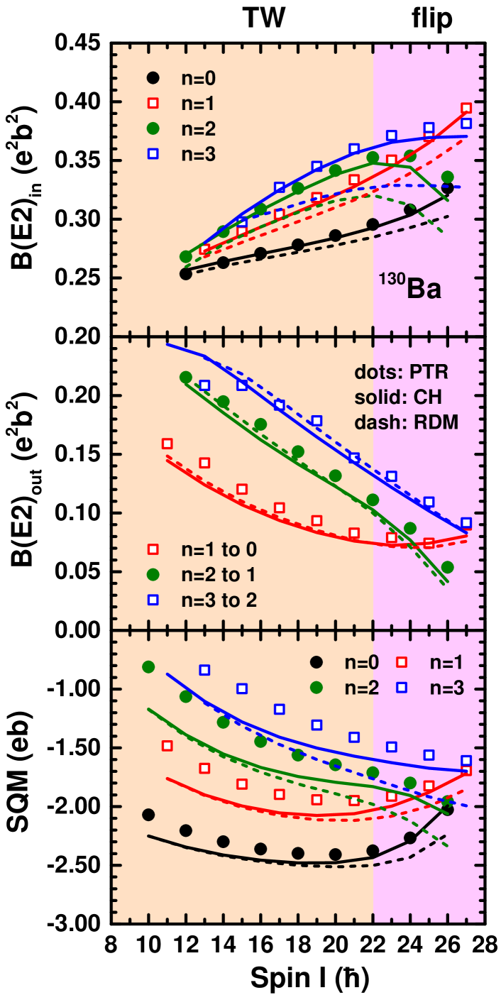
Figure 21: (Color online) Upper panel: In-band $B(E2)_{\textrm{in}}(I\to I-2)$ calculated by the PTR, CH, and sub-density matrix ($\rho^{(1)}$ or $\rho^{(2)}$, labeled as RDM) for the $n=0$, 1, 2, and 3 bands in ¹³⁰Ba. Middle panel: Inter-band $B(E2)_{\textrm{out}}(I\to I-1)$. Lower panel: Spectroscopic quadrupole moments $Q(I)$.

Figure 21 shows the electromagnetic transition probabilities and spectroscopic quadrupole moments (SQMs). The upper panel illustrates the in-band $B(E2)_{\textrm{in}}(I\to I-2)$ transition probabilities for the $n=0$, 1, 2, and 3 bands. The middle panel presents the inter-band $B(E2)_{\textrm{out}}(I\to I-1)$ transition probabilities among these bands. The strong collective $\Delta I=1$ $E2$ transitions associated with the wobbling motion are noted. For $B(E2)_{\textrm{in}}(I\to I-2)$ the CH values well agree with the PTR ones while for $B(E2)_{\textrm{out}}(I\to I-1)$ the CH values are slightly lower than the PTR ones. The results derived from the normalized sub-density matrix ($\rho^{(1)}$ or $\rho^{(2)}$, referred to as RDM), for $B(E2)_{\textrm{out}}(I\to I-1)$ are close to the CH values for all $I$. For the $n=0$ and 1 bands, the RDM $B(E2)_{\textrm{in}}(I\to I-2)$ values are somewhat lower than those from PTR and CH, with progressively larger deviations observed for the $n=2$ and 3 bands. This trend suggests that contributions from higher-order density matrices, particularly $\rho^{(3)}$ and $\rho^{(4)}$, become increasingly significant in the higher $n$ states.

The SQMs in the bottom panel increase with $n$. Both CH and RDM tend to underestimate the PTR results in the low-spin region, where they are close together. The deviations from the PTR values grow with $n$, which indicates that $\rho^{(3)}$ and $\rho^{(4)}$, become increasingly significant in the higher $n$ states. As the spin increases differences between these models emerge, with CH predictions converging to the PTR results. As already discussed in the preceding sections, the relations between the PTR, CH and RDM results can be elucidated by examining the SSS plots $P(\phi_{J})$ presented in Fig. 18.

VII Summary and Conclusions

We investigated the entanglement between the total and the quasi particle angular momenta, using the PTR model studies Chen and Frauendorf (2022, 2024) of ¹³⁵Pr and ¹³⁰Ba as examples for one and two quasiparticles coupled to a triaxial rotor. The study was carried out from two perspectives. The first starts from the bi-partition of the coupled system into the two subsystems, which are described by their respective reduced density matrices. The entanglement is quantified by the von Neumann (vN) entropy. It is found that the vN entropy $S$ increases with excitation energy, that is, the particle and total angular momenta become more entangled with the wobbling number $n$. The $S$ growths with the value of $I$ in the region of transverse wobbling (TW), because the Coriolis interaction becomes stronger. Above the critical spin, where the TW mode becomes unstable, $S$ does not change much with $I$, and the states group around $S/S^{(\textrm{max})}=0.7$ with no specific order, which is attributed to the smallness of the system.

Finite entropy implies a loss of coherence, that is the subsystems cannot be completely described by a wave function of their own. In order to characterize the decoherence we decomposed the reduced density matrices into their eigenstates, each of which representing a pure density matrix (or equivalently the wave function) of a rotor in the presence of one or two quasiparticles in a fixed quantum state, which can be viewed as the frozen alignment (FA) states of Ref. Frauendorf and Dönau (2014) with an individual effective particle angular momentum that is not completely alignde with the short axis.

We compared the probability distributions with respect to the angular momentum projection $K$ onto the long axis and of the angle $\phi_{J}$ of the angular momentum in the short-medium plane (spin squeezed states-SSS) of the full reduced density matrix with the pertaining distributions calculated from the sub-density matrices for each eigenstate. It turned out that to good approximation the full PTR probability distributions can be interpreted as the incoherent combination of the contributions from the first two pairs of eigenvectors of the reduced density matrix. The two states in each pair are even and odd linear combinations to the angular momentum vector with respect of the short-medium plane of the triaxial shape. Their probability distributions are almost identical.

We introduced the decoherence measures $\Delta_{K}$ and $\Delta_{\textrm{SSS}}$ which compare the probability distributions of the reduced density matrix with the “purified” distributions calculated from the square of the reduced density matrix. Their relative values scatter between 0.1 to 0.2 at low spin and between 0.1 and 0.3 at high spin. The values indicate a partially coherent density matrix, which is consistent with the plots of the distributions for each state.

The second perspective starts with the eigenstates of the collective Hamiltonian (CH) introduced in Ref. Chen and Frauendorf (2024), which accounts for the entanglement by assuming particle angular momentum $\bm{j}$ adiabatically follows the total angular momentum $\bm{J}$ such that the total energy is as small as possible. The $K$ and SSS probability distributions from the PTR reduced density matrix and sub-density matrixes were compared with the pertaining distributions from the CH eigenstates.

It is found that for ¹³⁵Pr the adiabatic approximation works well for the $n=$ 0 and 1 wobbling bands, marginally for $n=2$ band up to instability of the TW mode. Above it fails like for for $n=3$ band, which indicates that adiabaticity progressively deteriorates with $n$. When the CH provides a reasonable description, its distributions agree approximately with the scaled distributions calculated from the eigenstate pair of the reduced density matrix with the largest probability. This means that the collective wave function cannot provide a better description than the first pair of eigenstates. The remaining incoherent contributions become increasingly important with $n$.

For ¹³⁰Ba it is found that the CH provides a fair description of all wobbling bands $n=$0, 1, 2, 3, where the deviations of the CH dstributions from the PTR ones increase with $n$ as well. Within the considered spin range, which extends only to the $I$ values where the TW mode become unstable, the adiabatic approximation is more accurate for two quasiparticles coupled to the rotor than for one. The distributions $P_{\textrm{CH}}(K)$ agree with the corresponding scaled distributions calculated from the pair of sub-matrices with the largest weight in the PTR density matrix, which is found for ¹³⁵Pr alike when the adiabatic approximation is applicable. The SSS distributions $P_{\textrm{CH}}(\phi_{J})$ show a remarkable spin dependence. At low $I$ they are also close to the scaled distributions with the maximal weight. With increasing spin $P_{\textrm{CH}}(\phi_{J})$ approaches the distribution $P(\phi_{J})$ calculated from the complete reduced density.

In the TW regime the accuracy of the adiabatic approximation improves with spin because the wobbling energies go down. The smaller the excitation energies — the slower the collective motion — the better the adiabaticity. We attribute the spin dependence of $P_{\textrm{CH}}(\phi_{J})$ to this improvement of the approximation. The different $I$ dependence of $P_{\textrm{CH}}(K)$ is explained by the supposition that the motion is slow in $\phi_{J}$ and corresponding SSS basis states are as narrow as possible, which implies that they are distributed over the full $K$ range.

The electric $E2$ transition probabilities and spectroscopic quadrupole moments reflect the spin dependence of $P_{\textrm{CH}}(\phi_{J})$. At low $I$ they agree with the values from the pair of sub-density matrices with the largest weight, and they approach the PTR values from the complete reduced density matrix with increasing $I$. This is expected because the quadrupole operator is nearly local on the $\phi_{J}$ representation.

The conclusions obtained in the present study are to some extend specific to the PTR model. Nevertheless, many of the observed features result from the relative small dimensions of the entangled Hilbert spaces should apply to other coupled systems with comparable dimensions. It will be interesting to extend the present study to other exotic rotational modes, e.g., nuclear low-energy quadrupole modes Bohr and Mottelson (1975) and chiral rotation Frauendorf and Meng (1997) in the near future.

Appendix A Structure of the density matrices

In this Appendix, we compare $\rho^{(\textrm{CH})}$ with the mixed matrix $\rho$ and the pure sub-matrix $\rho^{(12)}$. The density matrices $\rho_{KK^{\prime}}$ and $\rho_{\phi_{J},\phi_{J}^{\prime}}$ are related to each other by the Fourier transform between the $K$ and $\phi_{J}$ representations. The matrix plots in Figs. 22 and 23 illustrate the relation for the PTR states $10_{1}$ and $26_{2}$ of ¹³⁰Ba. For each panel in Fig. 22, the $K$ values are ordered as $K=-I$, $-I+1$, …, $+I$ for both rows and columns. There are no matrix elements that connect even-$K$ basis states with odd-$K$ ones, which reflects the $\textrm{D}_{2}$ symmetry of the PTR Hamiltonian and of the CH. Accordingly, the eigenstates of the reduced density matrix appear in pairs of even-$K$ and odd-$K$ with nearly the same probability $p_{m}\approx p_{m+1}$. The third row’s panels show $\rho_{KK^{\prime}}^{(1)}$ of the first eigenstate of the PTR reduced density matrix, which includes only even-$K$ components. The second solution with odd-$K$ is added in the fourth row’s panels which show $\rho_{KK^{\prime}}^{(12)}$. As expected from the density of the plots, its $C_{l_{1}}$ norm is twice of that of $\rho_{KK^{\prime}}^{(1)}$. The second row’s panels show $\rho_{KK^{\prime}}^{(\textrm{CH})}$, which is the combination of the even-$K$ and odd-$K$ eigenstates of the CH. The matrix is nearly the same as $\rho_{KK^{\prime}}^{(12)}$, which holds for the diagonal shown in Fig. 19 as well. The two matrices differ from $\rho_{KK^{\prime}}$ shown in the in the first row’s panels, which includes $\rho_{KK^{\prime}}^{(34)}$ and the higher terms.

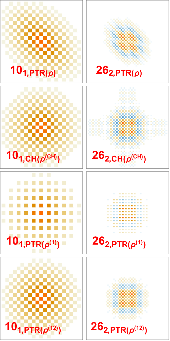
Figure 22: (Color online) Matrix plots of $\rho_{KK^{\prime}}$ for the $10_{1}$ and $26_{2}$ states in ¹³⁰Ba. First row: full density matrices $\rho_{KK^{\prime}}$ of PTR for the $10_{1}$ (left, $C_{l_{1}}=2.39$, $r_{C_{l_{1}}}=C_{l_{1}}/C_{l_{1}}^{(\textrm{max})}=C_{l_{1}}/2I=11.95\%$) and $26_{2}$ (right, $2.79$, $5.37\%$) states. Second row: density matrices $\rho_{KK^{\prime}}^{\textrm{(CH)}}$ (combination of even- and odd-$K$ solutions) of CH for the $10_{1}$ (left, $3.19$, $15.95\%$) and $26_{2}$ (right, $3.94$, $7.58\%$) states. Third row: sub-density matrices $\rho_{KK^{\prime}}^{(1)}$ of PTR for the $10_{1}$ (left, $1.27$, $6.35\%$) and $26_{2}$ (right, $1.39$, $2.68\%$) states. Fourth row: sub-density matrices $\rho_{KK^{\prime}}^{(12)}$ of PTR for the $10_{1}$ (left, $2.54$, $12.70\%$) and $26_{2}$ (right, $2.81$, $5.40\%$) states. For each plot, the $K$ values are ordered as $K=-I$, $-I+1$, …, $+I$ for both rows and columns. The color scale shows the zero values as white, the positive values as red, and the negative values as blue.

In our previous study Chen and Frauendorf (2024), we considered only the even-$K$ solutions. The odd-$K$ solutions have very similar energies and $E2$ matrix elements. Thus, to compare the results of PTR, the combination of even-$K$ and odd-$K$ solutions with equal weight of 1/2 for $10_{1}$ and $26_{2}$ states are shown in the second row’s panels of Fig. 22.

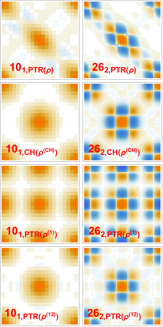
Figure 23: (Color online) Matrix plots of $\rho_{\phi_{m},\phi_{n}}$ for the $10_{1}$ and $26_{2}$ states in ¹³⁰Ba. First row: generated from the full density matrix $\rho_{KK^{\prime}}$ of PTR for the $10_{1}$ (left, $C_{l_{1}}=2.75$, $r_{C_{l_{1}}}=C_{l_{1}}/C_{l_{1}}^{(\textrm{max})}=C_{l_{1}}/2I=13.75\%$) and $26_{2}$ (right, $9.16$, $17.62\%$) states. Second row: generated from the density matrix $\rho_{KK^{\prime}}^{\textrm{(CH)}}$ (combination of even- and odd-$K$ solutions) of CH for the $10_{1}$ (left, $4.03$, $20.15\%$) and $26_{2}$ (right, $18.22$, $35.04\%$) states. Third row: generated from the sub-density matrix $\rho_{KK^{\prime}}^{(1)}$ of PTR for the $10_{1}$ (left, $3.25$, $16.25\%$) and $26_{2}$ (right, $9.16$, $17.62\%$) states. Fourth row: generated from the sub-density matrix $\rho_{KK^{\prime}}^{(12)}$ of PTR for the $10_{1}$ (left, $2.86$, $14.30\%$) and $26_{2}$ (right, $8.86$, $17.05\%$) states. For each plot, the angles $\phi_{n}=2n\pi/(2I+1)$ are ordered as $n=-I$, $-I+1$, …, $+I$ for both rows and columns. The color coding is the same as Fig. 22.

As discussed in Ref. Chen and Frauendorf (2024), the discrete SSS states form an orthonormal set, which is comprised of $2I+1$ angles of the angular momentum with respect to the 3-axis. The Eq. (40) transforms the basis from $|K\rangle$ states to the discrete SSS states $|\phi_{n}\rangle$. Figure 23 shows matrix plots of the density matrices $\rho_{\phi_{m},\phi_{n}}$ generated from the corresponding $\rho_{KK^{\prime}}$ in Fig. 22. These matrices are calculated using Eq. (32), where the discrete angles in the plots are defined as $\phi_{n}=2n\pi/(2I+1)$, with the order of $n=-I$, $-I+1$, …, $+I$ for rows and columns. The diagonal matrix elements of the respective matrices are a discrete selection of the pertaining functions $P(\phi_{J})$ and $P_{\textrm{CH}}(\phi_{J})$ in Fig. 18. The matrix elements in the corners of the panels reflect the symmetry of the PTR solutions.

The plot of the first eigenstate of the density matrix $\rho_{\phi_{m},\phi_{n}}^{(1)}$ (third row) well agrees with the plot of first eigenstate of the CH, which both involves only the even-$K$ basic states. We do not show the plot of the second eigenstate of the density matrix. It well agrees with the plot of second eigenstate of the CH (not shown), which involve only odd-$K$ basis states. The plots agree with the ones generated from the even-$K$ matrices, except that the matrix elements in regions around $(\phi_{m},\phi_{n})=(0,\pm\pi)$ and $(\pm\pi,0)$ have the opposite sign. These regions cancel each other when adding $\rho_{\phi_{m},\phi_{n}}^{(2)}$ to $\rho_{\phi_{m},\phi_{n}}^{(1)}$, which makes $\rho_{\phi_{m},\phi_{n}}^{(12)}$ (fourth row) more sparse than $\rho_{\phi_{m},\phi_{n}}^{(1)}$ (third row). Correspondingly, the $l_{1}$ norm $C_{l_{1}}$ of $\rho_{\phi_{m},\phi_{n}}^{(12)}$ is smaller than that of $\rho_{\phi_{m},\phi_{n}}^{(1)}$, and the entropy increases from 0 to $2\times\ln 2/\ln 21=0.46$. The matrix $\rho_{\phi_{m},\phi_{n}}^{(12)}$ is nearly identical with $\rho_{\phi_{m},\phi_{n}}^{(\textrm{CH})}$ (second row), which holds for the diagonal in Fig. 18 as well. The reduced density matrix of the PTR state $10_{1}$ (left of the first row) is also more sparse than the one generated from CH eigenstate (left of the second row), which corresponds to its larger entropy of $0.5\times\ln 21$. The reduction is generated by the terms $\rho_{\phi_{m},\phi_{n}}^{(34)}$ and higher.

As seen in Fig. 18, for $I=10$ the diagonal matrix elements $\rho_{\phi_{n},\phi_{n}}^{(12)}/(p_{1}+p_{2})$ and $\rho^{(\textrm{CH})}_{\phi_{n},\phi_{n}}$ are approximately equal. Both deviate from the full distribution $\rho_{\phi_{n},\phi_{n}}$, mainly by $\rho_{\phi_{n},\phi_{n}}^{(34)}/(p_{3}+p_{4})$. With increasing $I$, the diagonal matrix elements $\rho^{\textrm{(CH)}}_{\phi_{n},\phi_{n}}$ deviate from $\rho_{\phi_{n},\phi_{n}}^{(12)}/(p_{1}+p_{2})$ and approach $\rho_{\phi_{n},\phi_{n}}$.

The sub-matrices of the PTR state $26_{2}$ in the right column of Fig. 23 merge in an analog way as discussed for the matrices in the left column. Although the diagonal matrix element matrix elements of $\rho^{\textrm{(CH)}}_{\phi_{m},\phi_{n}}$ are very close to the ones of $\rho_{\phi_{m},\phi_{n}}$ (see Fig. 18), the full matrices differ from each other. The elements of reduced density matrix (right of the first row) are concentrated around the diagonal, which reflects the relative large entropy of $0.6\times\ln 21$. The density matrix of the corresponding paired eigenstates of the CH (right of the second row) has elements that are more spread over its range, which is needed to satisfy the purity condition $\rho^{2}=\rho$ for each of the two eigenstates. The entropy is $2\ln 2=0.46\ln 21$, because a pair of matrices is combined.

Appendix B Quadrupole moment matrix elements

In this Appendix, we provide the results of quadrupole moment matrix elements.

Figure 24: (Color online) Matrix elements of $\hat{Q}_{0}$ (upper panels) and $\hat{Q}_{2}+\hat{Q}_{-2}$ (lower panels) operators on the basis $|\phi_{n}\rangle$ with $\phi_{n}=2n\pi/(2I+1)$ and $n=-I$, $-I+1$, …, $+I$ for $I=10$ (left panels) and $26$ (right panels) in ¹³⁰Ba. The color scale shows the zero values as white, the positive values as red, orange, and yellow, and the negative values as blue and light blue.

The matrix elements of quadrupole operators $\hat{Q}_{0}$ and $\hat{Q}_{2}+\hat{Q}_{-2}$ on the basis of $|\phi_{n}\rangle$ are shown in Fig. 24. In the $K$-basis, the transition matrix elements of $\hat{Q}_{0}$ and $\hat{Q}_{2}+\hat{Q}_{-2}$ are calculated as Bohr and Mottelson (1975)

$$\langle I^{\prime},K^{\prime}|\hat{Q}_{0}|I,K\rangle=Q_{20}^{\prime}\langle IK20|I^{\prime}K^{\prime}\rangle,\quad K^{\prime}=K,$$ (48)

$$\langle I^{\prime},K^{\prime}|\hat{Q}_{2}+\hat{Q}_{-2}|I,K\rangle=Q_{22}^{\prime}\Big{[}\langle IK22|I^{\prime}K^{\prime}\rangle+\langle IK2-2|I^{\prime}K^{\prime}\rangle\Big{]},$$

$$\quad\quad\quad\quad\quad\quad\quad\quad\quad\quad\quad\quad\quad\quad\quad K^{\prime}=K\pm 2,$$ (49)

with the intrinsic quadrupole moment $Q_{20}^{\prime}=Q_{0}^{\prime}\cos\gamma$ and $Q_{22}^{\prime}=Q_{0}^{\prime}\sin\gamma/\sqrt{2}$ ($Q_{0}^{\prime}$ is an empirical quadrupole moment that is related to the axial deformation $\beta$). In addition, $I$ is the initial spin value and the final spin $I^{\prime}$ can be taken as $I$, $I\pm 1$, and $I\pm 2$. In the discrete SSS representation $|\phi_{n}\rangle$, which is complete orthonormal, we need transform the above matrix elements to the SSS basis using the following relationship Chen and Frauendorf (2024)

$$|I,\phi_{n}\rangle =\frac{1}{\sqrt{2I+1}}\sum_{K=-I}^{I}e^{iK\phi_{n}}|I,K\rangle.$$ (50)

In detail, the matrix elements of quadrupole operators on the basis of $|\phi_{n}\rangle$ are calculated as

$$\quad\langle I^{\prime},\phi_{m}|\hat{Q}_{0}|I,\phi_{n}\rangle$$

$$=\frac{1}{\sqrt{2I^{\prime}+1}}\frac{1}{\sqrt{2I+1}}Q_{20}^{\prime}\sum_{K}e^{i(K\phi_{n}-K\phi_{m})}\langle IK20|I^{\prime}K\rangle,$$ (51)

$$\quad\langle I^{\prime},\phi_{m}|\hat{Q}_{2}+\hat{Q}_{-2}|I,\phi_{n}\rangle$$

$$=\frac{1}{\sqrt{2I^{\prime}+1}}\frac{1}{\sqrt{2I+1}}Q_{22}^{\prime}\sum_{K}\Big{[}e^{i[K\phi_{n}-(K+2)\phi_{m}]}\langle IK22|I^{\prime}K+2\rangle$$

$$\quad+e^{i[K\phi_{n}-(K-2)\phi_{m}]}\langle IK2-2|I^{\prime}K-2\rangle\Big{]}.$$ (52)

Since the matrix elements for the cases of $I^{\prime}=I$, $I\pm 1$, and $I\pm 2$ look similar, Fig. 24 only shows the matrix elements for the case of $I^{\prime}=I$. For each plot, the angles $\phi_{n}=2n\pi/(2I+1)$ are ordered as $n=-I$, $-I+1$, …, $+I$ for both rows and columns. Figure 24 illustrates that the matrix elements of $\hat{Q}_{0}$ and $\hat{Q}_{2}+\hat{Q}_{-2}$ on the basis of $|\phi_{n}\rangle$ are much more denser than those on the basis of $|K\rangle$, where the $\hat{Q}_{0}$ and $\hat{Q}_{2}+\hat{Q}_{-2}$ have matrix elements only when $K^{\prime}=K$ and $K^{\prime}=K\pm 2$, respectively.

However, it should be noted that the only matrix elements close to the diagonal are significant when evaluating the trace of the product of a quadrupole matrix with a density matrix, because those further away have much smaller values and display an oscillatory behavior. To a good approximation one can replace the traces by integrals over the various probability densities times the classical values

$$\hat{Q_{0}}=-Q^{\prime}_{20}/2,\quad\hat{Q}_{2}+\hat{Q}_{-2}=Q^{\prime}_{22}\sqrt{3/2}\cos 2\phi_{J}.$$ (53)

The fact that the near-diagonal matrix elements of $\rho^{\textrm{(CH)}}_{\phi_{m},\phi_{n}}$ are close to the ones of $\rho_{\phi_{m},\phi_{n}}$ provides an intuitive interpretation of structure of the state. However, the CH wave function describes the $E2$ matrix elements between the PTR states only with the accuracy of $P_{12}(K)/(p_{1}+p_{2})$ because the intrinsic quadrupole operator $\hat{Q}_{0}$ has only diagonal matrix elements, and the matrix elements of $\hat{Q}_{2}+\hat{Q}_{-2}$ are restricted to the region $\Delta K=\pm 2$ around the diagonal of $\rho_{KK^{\prime}}^{(12)}$. The $E2$ matrix elements between the PTR states do not depend on the chosen basis. The closeness of near-diagonal matrix matrix elements of $\rho^{\textrm{(CH)}}_{\phi_{m},\phi_{n}}$ to the ones of $\rho_{\phi_{m},\phi_{n}}$ is offset by wide distribution of the matrices $\hat{Q}_{0}$ and $\hat{Q}_{2}+\hat{Q}_{-2}$ in the $\phi_{n}$ basis when calculating $\mathrm{Tr}\left(\hat{Q}_{0}\rho^{(\textrm{CH})}\right)$ and $\mathrm{Tr}\left[(\hat{Q}_{2}+\hat{Q}_{-2})\rho^{(\textrm{CH})}\right]$. The expressions and an illustration are given in the Appendix A. Nevertheless as seen in Fig. 24, the eigenstates of the CH quite well reproduce the $B(E2)$ values of the PTR states.

References

- Bohr and Mottelson (1975) A. Bohr and B. R. Mottelson, Nuclear structure, Vol. II (Benjamin, New York, 1975).
- Frauendorf and Dönau (2014) S. Frauendorf and F. Dönau, Phys. Rev. C 89, 014322 (2014).
- Chen and Frauendorf (2022) Q. B. Chen and S. Frauendorf, Eur. Phys. J. A 58, 75 (2022).
- Chen and Frauendorf (2024) Q. B. Chen and S. Frauendorf, Phys. Rev. C 109, 044304 (2024).
- Ødegård et al. (2001) S. W. Ødegård, G. B. Hagemann, D. R. Jensen, M. Bergström, B. Herskind, G. Sletten, S. Törmänen, J. N. Wilson, P. O. Tjøm, I. Hamamoto, K. Spohr, H. Hübel, A. Görgen, G. Schönwasser, A. Bracco, S. Leoni, A. Maj, C. M. Petrache, P. Bednarczyk, and D. Curien, Phys. Rev. Lett. 86, 5866 (2001).
- Matta et al. (2015) J. T. Matta, U. Garg, W. Li, S. Frauendorf, A. D. Ayangeakaa, D. Patel, K. W. Schlax, R. Palit, S. Saha, J. Sethi, T. Trivedi, S. S. Ghugre, R. Raut, A. K. Sinha, R. V. F. Janssens, S. Zhu, M. P. Carpenter, T. Lauritsen, D. Seweryniak, C. J. Chiara, F. G. Kondev, D. J. Hartley, C. M. Petrache, S. Mukhopadhyay, D. V. Lakshmi, M. K. Raju, P. V. Madhusudhana Rao, S. K. Tandel, S. Ray, and F. Dönau, Phys. Rev. Lett. 114, 082501 (2015).
- Sensharma et al. (2020) N. Sensharma, U. Garg, Q. B. Chen, S. Frauendorf, D. P. Burdette, J. L. Cozzi, K. B. Howard, S. Zhu, M. P. Carpenter, P. Copp, F. G. Kondev, T. Lauritsen, J. Li, D. Seweryniak, J. Wu, A. D. Ayangeakaa, D. J. Hartley, R. V. F. Janssens, A. M. Forney, W. B. Walters, S. S. Ghugre, and R. Palit, Phys. Rev. Lett. 124, 052501 (2020).
- Guo et al. (2024) R. J. Guo, S. Y. Wang, C. Liu, R. A. Bark, J. Meng, S. Q. Zhang, B. Qi, A. Rohilla, Z. H. Li, H. Hua, Q. B. Chen, H. Jia, X. Lu, S. Wang, D. P. Sun, X. C. Han, W. Z. Xu, E. H. Wang, H. F. Bai, M. Li, P. Jones, J. F. Sharpey-Schafer, M. Wiedeking, O. Shirinda, C. P. Brits, K. L. Malatji, T. Dinoko, J. Ndayishimye, S. Mthembu, S. Jongile, K. Sowazi, S. Kutlwano, T. D. Bucher, D. G. Roux, A. A. Netshiya, L. Mdletshe, S. Noncolela, and W. Mtshali, Phys. Rev. Lett. 132, 092501 (2024).
- Timár et al. (2019) J. Timár, Q. B. Chen, B. Kruzsicz, D. Sohler, I. Kuti, S. Q. Zhang, J. Meng, P. Joshi, R. Wadsworth, K. Starosta, A. Algora, P. Bednarczyk, D. Curien, Z. Dombrádi, G. Duchêne, A. Gizon, J. Gizon, D. G. Jenkins, T. Koike, A. Krasznahorkay, J. Molnár, B. M. Nyakó, E. S. Paul, G. Rainovski, J. N. Scheurer, A. J. Simons, C. Vaman, and L. Zolnai, Phys. Rev. Lett. 122, 062501 (2019).
- Sensharma et al. (2019) N. Sensharma, U. Garg, S. Zhu, A. D. Ayangeakaa, S. Frauendorf, W. Li, G. Bhat, J. A. Sheikh, M. P. Carpenter, Q. B. Chen, J. L. Cozzi, S. S. Ghugre, Y. K. Gupta, D. J. Hartley, K. B. Howard, R. V. F. Janssens, F. G. Kondev, T. C. McMaken, R. Palit, J. Sethi, D. Seweryniak, and R. P. Singh, Phys. Lett. B 792, 170 (2019).
- Biswas et al. (2019) S. Biswas, R. Palit, S. Frauendorf, U. Garg, W. Li, G. H. Bhat, J. A. Sheikh, J. Sethi, S. Saha, P. Singh, D. Choudhury, J. T. Matta, A. D. Ayangeakaa, W. A. Dar, V. Singh, and S. Sihotra, Eur. Phys. J. A 55, 159 (2019).
- Petrache et al. (2019) C. M. Petrache, P. M. Walker, S. Guo, Q. B. Chen, S. Frauendorf, Y. X. Liu, R. A. Wyss, D. Mengoni, Y. H. Qiang, A. Astier, E. Dupont, R. Li, B. F. Lv, K. K. Zheng, D. Bazzacco, A. Boso, A. Goasduff, F. Recchia, D. Testov, F. Galtarossa, G. Jaworski, D. R. Napoli, S. Riccetto, M. Siciliano, J. J. Valiente-Dobon, M. L. Liu, X. H. Zhou, J. G. Wang, C. Andreoiu, F. H. Garcia, K. Ortner, K. Whitmore, T. Back, B. Cederwall, E. A. Lawrie, I. Kuti, D. Sohler, J. Timár, T. Marchlewski, J. Srebrny, and A. Tucholski, Phys. Lett. B 795, 241 (2019).
- Chen et al. (2019) Q. B. Chen, S. Frauendorf, and C. M. Petrache, Phys. Rev. C 100, 061301(R) (2019).
- Chakraborty et al. (2020) S. Chakraborty, H. P. Sharma, S. S. Tiwary, C. Majumder, A. K. Gupta, P. Banerjee, S. Ganguly, S. Rai, Pragati, Mayank, S. Kumar, A. Kumar, R. Palit, S. S. Bhattacharjee, R. P. Singh, and S. Muralithar, Phys. Lett. B 811, 135854 (2020).
- Rojeeta Devi et al. (2021) K. Rojeeta Devi, S. Kumar, N. Kumar, Neelam, F. S. Babra, M. S. R. Laskar, S. Biswas, S. Saha, P. Singh, S. Samanta, S. Das, S. Chakraborty, R. P. Singh, S. Muralithar, and A. Kumar, Phys. Lett. B 823, 136756 (2021).
- Lv et al. (2022) B. F. Lv, C. M. Petrache, R. Budaca, A. Astier, K. K. Zheng, P. Greenlees, H. Badran, T. Calverley, D. M. Cox, T. Grahn, J. Hilton, R. Julin, S. Juutinen, J. Konki, J. Pakarinen, P. Papadakis, J. Partanen, P. Rahkila, P. Ruotsalainen, M. Sandzelius, J. Saren, C. Scholey, J. Sorri, S. Stolze, J. Uusitalo, B. Cederwall, A. Ertoprak, H. Liu, S. Guo, J. G. Wang, H. J. Ong, X. H. Zhou, Z. Y. Sun, I. Kuti, J. Timár, A. Tucholski, J. Srebrny, and C. Andreoiu, Phys. Rev. C 105, 034302 (2022).
- Prajapati et al. (2024) M. Prajapati, S. Nag, A. K. Singh, A. Al-Khatib, H. Hübel, A. Neußer-Neffgen, G. B. Hagemann, G. Sletten, B. Herskind, C. R. Hansen, G. Benzoni, A. Bracco, R. V. F. Janssens, M. P. Carpenter, and P. Chowdhury, Phys. Rev. C 109, 034301 (2024).
- Jensen et al. (2002) D. R. Jensen, G. B. Hagemann, I. Hamamoto, S. W. Ødegård, B. Herskind, G. Sletten, J. N. Wilson, K. Spohr, H. Hübel, P. Bringel, A. Neußer, G. Schönwaßer, A. K. Singh, W. C. Ma, H. Amro, A. Bracco, S. Leoni, G. Benzoni, A. Maj, C. M. Petrache, G. L. Bianco, P. Bednarczyk, and D. Curien, Phys. Rev. Lett. 89, 142503 (2002).
- Bringel et al. (2005) P. Bringel, G. B. Hagemann, H. Hübel, A. Al-khatib, P. Bednarczyk, A. Bürger, D. Curien, G. Gangopadhyay, B. Herskind, D. R. Jensen, D. T. Joss, T. Kröll, G. Lo Bianco, S. Lunardi, W. C. Ma, N. Nenoff, A. Neußer-Neffgen, C. M. Petrache, G. Schönwasser, J. Simpson, A. K. Singh, N. Singh, and G. Sletten, Eur. Phys. J. A 24, 167 (2005).
- Schönwaßer et al. (2003) G. Schönwaßer, H. Hübel, G. B. Hagemann, P. Bednarczyk, G. Benzoni, A. Bracco, P. Bringel, R. Chapman, D. Curien, J. Domscheit, B. Herskind, D. R. Jensen, S. Leoni, G. Lo Bianco, W. C. Ma, A. Maj, A. Neusser, S. W. Ødegård, C. M. Petrache, D. Rossach, H. Ryde, K. H. Spohr, and A. K. Singh, Phys. Lett. B 552, 9 (2003).
- Amro et al. (2003) H. Amro, W. C. Ma, G. B. Hagemann, R. M. Diamond, J. Domscheit, P. Fallon, A. Gorgen, B. Herskind, H. Hübel, D. R. Jensen, Y. Li, A. O. Macchiavelli, D. Roux, G. Sletten, J. Thompson, D. Ward, I. Wiedenhover, J. N. Wilson, and J. A. Winger, Phys. Lett. B 553, 197 (2003).
- Hartley et al. (2009) D. J. Hartley, R. V. F. Janssens, L. L. Riedinger, M. A. Riley, A. Aguilar, M. P. Carpenter, C. J. Chiara, P. Chowdhury, I. G. Darby, U. Garg, Q. A. Ijaz, F. G. Kondev, S. Lakshmi, T. Lauritsen, A. Ludington, W. C. Ma, E. A. McCutchan, S. Mukhopadhyay, R. Pifer, E. P. Seyfried, I. Stefanescu, S. K. Tandel, U. Tandel, J. R. Vanhoy, X. Wang, S. Zhu, I. Hamamoto, and S. Frauendorf, Phys. Rev. C 80, 041304(R) (2009).
- Mukherjee et al. (2023) A. Mukherjee, S. Bhattacharya, T. Trivedi, S. Tiwari, R. P. Singh, S. Muralithar, Yashraj, K. Katre, R. Kumar, R. Palit, S. Chakraborty, S. Jehangir, N. Nazir, S. P. Rouoof, G. H. Bhat, J. A. Sheikh, N. Rather, R. Raut, S. S. Ghugre, S. Ali, S. Rajbanshi, S. Nag, S. S. Tiwary, A. Sharma, S. Kumar, S. Yadav, and A. K. Jain, Phys. Rev. C 107, 054310 (2023).
- Nandi et al. (2020) S. Nandi, G. Mukherjee, Q. B. Chen, S. Frauendorf, R. Banik, S. Bhattacharya, S. Dar, S. Bhattacharyya, C. Bhattacharya, S. Chatterjee, S. Das, S. Samanta, R. Raut, S. S. Ghugre, S. Rajbanshi, S. Ali, H. Pai, M. A. Asgar, S. Das Gupta, P. Chowdhury, and A. Goswami, Phys. Rev. Lett. 125, 132501 (2020).
- Frauendorf (2024) S. Frauendorf, arXiv: nucl-th, 2405.02747 (2024).
- Sun et al. (2024) B. W. Sun, Y. Z. Ji, and Q. B. Chen, Nucl. Phys. Rev. 41, 200 (2024).
- Hamamoto (2002) I. Hamamoto, Phys. Rev. C 65, 044305 (2002).
- Hamamoto and Mottelson (2003) I. Hamamoto and B. R. Mottelson, Phys. Rev. C 68, 034312 (2003).
- Streck et al. (2018) E. Streck, Q. B. Chen, N. Kaiser, and U.-G. Meißner, Phys. Rev. C 98, 044314 (2018).
- Chen et al. (2020) Q. B. Chen, S. Frauendorf, N. Kaiser, U.-G. Meißner, and J. Meng, Phys. Lett. B 807, 135596 (2020).
- Broocks et al. (2021) C. Broocks, Q. B. Chen, N. Kaiser, and U.-G. Meißner, Eur. Phys. J. A 57, 161 (2021).
- Hu et al. (2021) L. Hu, J. Peng, and Q. B. Chen, Phys. Rev. C 104, 064325 (2021).
- Li et al. (2022) W. C. Li, S. Frauendorf, and M. A. Caprio, Eur. Phys. J. A 58, 218 (2022).
- Dai et al. (2023) H. M. Dai, Q. B. Chen, and X.-R. Zhou, Phys. Rev. C 108, 054306 (2023).
- Li et al. (2024) S. H. Li, H. M. Dai, Q. B. Chen, and X.-R. Zhou, Chin. Phys. C 48, 034102 (2024).
- Dai and Chen (2024) H. M. Dai and Q. B. Chen, Phys. Rev. C 109, 054321 (2024).
- Tanabe and Sugawara-Tanabe (2017) K. Tanabe and K. Sugawara-Tanabe, Phys. Rev. C 95, 064315 (2017).
- Raduta et al. (2017) A. A. Raduta, R. Poenaru, and L. G. Ixaru, Phys. Rev. C 96, 054320 (2017).
- Budaca (2018) R. Budaca, Phys. Rev. C 97, 024302 (2018).
- Lawrie et al. (2020) E. A. Lawrie, O. Shirinda, and C. M. Petrache, Phys. Rev. C 101, 034306 (2020).
- Budaca (2021) R. Budaca, Phys. Rev. C 103, 044312 (2021).
- Raduta et al. (2021) A. A. Raduta, C. M. Raduta, and R. Poenaru, J. Phys. G: Nucl. Part. Phys. 48, 015106 (2021).
- Raduta et al. (2022) C. M. Raduta, A. A. Raduta, R. Poenaru, and A. H. Raduta, J. Phys. G: Nucl. Part. Phys. 49, 025105 (2022).
- Budaca and Petrache (2022) R. Budaca and C. M. Petrache, Phys. Rev. C 106, 014313 (2022).
- Marshalek (1979) E. R. Marshalek, Nucl. Phys. A 331, 429 (1979).
- Shimizu and Matsuzaki (1995) Y. R. Shimizu and M. Matsuzaki, Nucl. Phys. A 588, 559 (1995).
- Matsuzaki et al. (2002) M. Matsuzaki, Y. R. Shimizu, and K. Matsuyanagi, Phys. Rev. C 65, 041303 (2002).
- Matsuzaki et al. (2004a) M. Matsuzaki, Y. R. Shimizu, and K. Matsuyanagi, Phys. Rev. C 69, 034325 (2004a).
- Matsuzaki and Ohtsubo (2004) M. Matsuzaki and S. Ohtsubo, Phys. Rev. C 69, 064317 (2004).
- Matsuzaki et al. (2004b) M. Matsuzaki, Y. R. Shimizu, and K. Matsuyanagi, Eur. Phys. J. A 20, 189 (2004b).
- Shimizu et al. (2004) Y. R. Shimizu, M. M. Matsuzaki, and K. Matsuyanagi, arXiv nucl-th, 0404063v1 (2004).
- Shimizu et al. (2005) Y. R. Shimizu, M. Matsuzaki, and K. Matsuyanagi, Phys. Rev. C 72, 014306 (2005).
- Almehed et al. (2006) D. Almehed, R. G. Nazmitdinov, and F. Doenau, Phys. Scr. T125, 139 (2006).
- Shimizu et al. (2008) Y. R. Shimizu, T. Shoji, and M. Matsuzaki, Phys. Rev. C 77, 024319 (2008).
- Shoji and Shimizu (2009) T. Shoji and Y. R. Shimizu, Progr. Theor. Phys. 121, 319 (2009).
- Frauendorf and Dönau (2015) S. Frauendorf and F. Dönau, Phys. Rev. C 92, 064306 (2015).
- Chen et al. (2014) Q. B. Chen, S. Q. Zhang, P. W. Zhao, and J. Meng, Phys. Rev. C 90, 044306 (2014).
- Chen et al. (2016) Q. B. Chen, S. Q. Zhang, and J. Meng, Phys. Rev. C 94, 054308 (2016).
- Shimada et al. (2018) M. Shimada, Y. Fujioka, S. Tagami, and Y. R. Shimizu, Phys. Rev. C 97, 024318 (2018).
- Wang et al. (2020) Y. K. Wang, F. Q. Chen, and P. W. Zhao, Phys. Lett. B 802, 135246 (2020).
- Chen and Petrache (2021) F.-Q. Chen and C. M. Petrache, Phys. Rev. C 103, 064319 (2021).
- Calabrese and Cardy (2004) P. Calabrese and J. Cardy, J. Stat. Mech: Theory Exp. 2004, P06002 (2004).
- Amico et al. (2008) L. Amico, R. Fazio, A. Osterloh, and V. Vedral, Rev. Mod. Phys. 80, 517 (2008).
- Peschel and Eisler (2009) I. Peschel and V. Eisler, J. Phys. A: Math. Theor. 42, 504003 (2009).
- Horodecki et al. (2009) R. Horodecki, P. Horodecki, M. Horodecki, and K. Horodecki, Rev. Mod. Phys. 81, 865 (2009).
- Nishioka et al. (2009) T. Nishioka, S. Ryu, and T. Takayanagi, J. Phys. A: Math. Theor. 42, 504008 (2009).
- Eisert et al. (2010) J. Eisert, M. Cramer, and M. B. Plenio, Rev. Mod. Phys. 82, 277 (2010).
- Lin and Radičević (2020) J. Lin and D. Radičević, Nucl. Phys. B 958, 115118 (2020).
- Kanada-En’yo (2015a) Y. Kanada-En’yo, Phys. Rev. C 91, 034303 (2015a).
- Legeza et al. (2015) O. Legeza, L. Veis, A. Poves, and J. Dukelsky, Phys. Rev. C 92, 051303 (2015).
- Kanada-En’yo (2015b) Y. Kanada-En’yo, Prog. Theor. Exp. Phys. 2015, 043D04 (2015b).
- Kanada-En’yo (2015c) Y. Kanada-En’yo, Prog. Theor. Exp. Phys. 2015, 051D01 (2015c).
- Beane et al. (2019) S. R. Beane, D. B. Kaplan, N. Klco, and M. J. Savage, Phys. Rev. Lett. 122, 102001 (2019).
- Robin et al. (2021) C. Robin, M. J. Savage, and N. Pillet, Phys. Rev. C 103, 034325 (2021).
- Faba et al. (2021) J. Faba, V. Martín, and L. Robledo, Phys. Rev. A 104, 032428 (2021).
- Kruppa et al. (2022) A. T. Kruppa, J. Kovács, P. Salamon, O. Legeza, and G. Zaránd, Phys. Rev. C 106, 024303 (2022).
- Pazy (2023) E. Pazy, Phys. Rev. C 107, 054308 (2023).
- Bai and Ren (2022) D. Bai and Z. Z. Ren, Phys. Rev. C 106, 064005 (2022).
- Lacroix et al. (2022) D. Lacroix, A. B. Balantekin, M. J. Cervia, A. V. Patwardhan, and P. Siwach, Phys. Rev. D 106, 123006 (2022).
- Tichai et al. (2023) A. Tichai, S. Knecht, A. T. Kruppa, O. Legeza, C. P. Moca, A. Schwenk, M. A. Werner, and G. Zarand, Phys. Lett. B 845, 138139 (2023).
- Bulgac et al. (2023) A. Bulgac, M. Kafker, and I. Abdurrahman, Phys. Rev. C 107, 044318 (2023).
- Bulgac (2023) A. Bulgac, Phys. Rev. C 107, L061602 (2023).
- Johnson and Gorton (2023) C. W. Johnson and O. C. Gorton, J. Phys. G: Nucl. Part. Phys. 50, 045110 (2023).
- Gu et al. (2023) C. Y. Gu, Z. H. Sun, G. Hagen, and T. Papenbrock, Phys. Rev. C 108, 054309 (2023).
- von Neumann (1927) J. von Neumann, Gött. Nach. 1, 273 (1927).
- Landau (1927) L. Landau, Z. Phys. 45, 430 (1927).
- Born et al. (1999) M. Born, E. Wolf, A. B. Bhatia, P. C. Clemmow, D. Gabor, A. R. Stokes, A. M. Taylor, P. A. Wayman, and W. L. Wilcock, Principles of Optics: Electromagnetic Theory of Propagation, Interference and Diffraction of Light, 7th ed. (Cambridge University Press, 1999).
- Hecht (1998) E. Hecht, Optics, Addison-Wesley world student series (Addison-Wesley, 1998).
- Nielsen and Chuang (2010) M. Nielsen and I. Chuang, Quantum Computation and Quantum Information: 10th Anniversary Edition (Cambridge University Press, Cambridge, 2010).
- Tichy et al. (2011) M. C. Tichy, F. Mintert, and A. Buchleitner, J. Phys. B: At., Mol. Opt. Phys. 44, 192001 (2011).
- Vedral et al. (1997) V. Vedral, M. B. Plenio, M. A. Rippin, and P. L. Knight, Phys. Rev. Lett. 78, 2275 (1997).
- Baumgratz et al. (2014) T. Baumgratz, M. Cramer, and M. B. Plenio, Phys. Rev. Lett. 113, 140401 (2014).
- Frauendorf and Meng (1996) S. Frauendorf and J. Meng, Z. Phys. A 356, 263 (1996).
- Ring and Schuck (1980) P. Ring and P. Schuck, The nuclear many body problem (Springer Verlag, Berlin, 1980).
- Frauendorf and Meng (1997) S. Frauendorf and J. Meng, Nucl. Phys. A 617, 131 (1997).