Last-iterate Convergence in Regularized Graphon Mean Field Game

Abstract

To model complex real-world systems, such as traders in stock markets, or the dissemination of contagious diseases, graphon mean-field games (GMFG) have been proposed to model many agents. Despite the empirical success, our understanding of GMFG is limited. Popular algorithms such as mirror descent are deployed but remain unknown for their convergence properties. In this work, we give the first last-iterate convergence rate of mirror descent in regularized monotone GMFG. In tabular monotone GMFG with finite state and action spaces and under bandit feedback, we show a last-iterate convergence rate of $O(T^{-1/4})$. Moreover, when exact knowledge of costs and transitions is available, we improve this convergence rate to $O(T^{-1})$, matching the existing convergence rate observed in strongly convex games. In linear GMFG, our algorithm achieves a last-iterate convergence rate of $O(T^{-1/5})$. Finally, we verify the performance of the studied algorithms by empirically testing them against fictitious play in a variety of tasks.

1 Introduction

In many real-world applications, the presence of complex systems including many interacting individuals or components is indispensable. These systems manifest in various forms, from the intricate networks of neurons within human brains (Bullmore and Sporns,, 2009, 2012; Avena-Koenigsberger et al.,, 2018), to the dynamic interactions of traders in stock markets (Bakker et al.,, 2010; Bian et al.,, 2016), and to the dissemination of contagious diseases throughout societies (Newman,, 2002; Pastor-Satorras et al.,, 2015). Due to the large number of interacting individuals or components, these systems pose significant challenges for modeling. Mean field games (MFG) (Caines et al.,, 2006; Lasry and Lions,, 2007) have emerged as a highly effective approach for addressing this complexity, offering both scalability and robust theoretical guarantees in these multi-agent systems. MFG operates on the principle of weak interactions, positing that each individual’s influence on the overall system is negligible. This framework has been successfully applied to many real-world tasks, including social networks (Yang et al.,, 2018), and swarm robotics (Cui et al.,, 2023).

The MFG framework leverages the assumption of agent homogeneity and has demonstrated success across various applications. However, this assumption becomes a hindrance when dealing with heterogeneous agents. To address this limitation, the Graphon mean field games (GMFG) Parise and Ozdaglar, (2019); Aurell et al., (2022) framework has been introduced as an extension of MFGs to accommodate heterogeneous agent modeling. The GMFG framework captures agent interactions through a graphical structure and is shown to be successful in applications like modeling investment decisions in financial markets (Tangpi and Zhou,, 2024). Despite the empirical success of MFG and GMFG, our theoretical understanding of this framework remains limited.

In monotone MFGs (Lasry and Lions,, 2007), and under the access to the exact cost and transition functions, Perrin et al., (2020) proposed a continuous time fictitious play algorithm, where the averaged iterates policy converge to a Nash equilibrium in $O(T^{-1})$ iterations. For discrete-time monotone GMFGs with access to exact cost and transition functions, Zhang et al., (2023) proposed a mirror descent-based algorithm that converges to the Nash equilibrium in $O(T^{-1/2})$ iterations.

However, in real-world applications, approximating continuous-time dynamics can be challenging, and exact knowledge of cost and transition functions may not be feasible. Agents typically only receive bandit feedback, meaning they observe the cost and transitions associated with the states and actions they have visited. Meanwhile, the existing approaches only guarantee the convergence of the time average of the joint action profile, rather than the last-iterate convergence, the convergence of the joint action profile. Last-iterate convergence holds greater appeal as it offers a descriptive account of the evolution of players’ overall behavior. In contrast, while the trajectory of players’ joint action converge in the time-average sense, it may exhibit cycling, which is not suitable for practical deployment (Mertikopoulos et al.,, 2018). The following question thus arises.

How fast can discrete-time algorithms converge (in the last iterate) to a Nash equilibrium in GMFGs with bandit feedback?

In this work, we focus on the mirror descent-based algorithm, which has been empirically verified to be successful in GMFGs (Pérolat et al.,, 2022; Zhang et al.,, 2023). In tabular monotone GMFGs (finite state and actions space) and under bandit feedback, we show a $O(T^{-1/4})$ last-iterate convergence rate. When the exact knowledge of cost and transitions is present, we show that the convergence rate can be improved to $O(T^{-1})$, matching the existing convergence rate in strongly convex (but not mean field) games. To address scenarios involving large or even infinite state spaces, we extend our analysis to linear GMFGs, where costs and transitions adhere to a linear structure. In this context, we achieve a last-iterate convergence rate of $O(T^{-1/5})$. We validate the effectiveness of the studied algorithm by empirically comparing them against the fictitious play in four different environments.

2 Related Works

Mean Field Game (MFG)

To address the challenge of modeling a large number of agents in a game, the Mean Field Game (MFG) was proposed by Caines et al., (2006); Lasry and Lions, (2007). It considers the limit case of a continuous distribution of homogeneous agents (all anonymous and with symmetric interest) and reduces the problem to the characterization of the optimal behavior of a single representative agent. The classic approaches include the numerical approximation approach for partial differential equation (Achdou and Capuzzo-Dolcetta,, 2010; Achdou et al.,, 2012, 2020), and the more recent deep reinforcement learning approaches (Cui and Koeppl, 2021a, ; Lauriere et al.,, 2022; Fabian et al.,, 2023).

Recent efforts also introduced the traditional fictitious play (FP) algorithm and combined it with machine learning techniques (Perrin et al.,, 2020). While FP achieves impressive results and is shown to be convergent (Geist et al.,, 2022), it is hard to scale due to its low computational efficiency, as it requires computing the best response at every iteration. To address this, the policy mirror descent algorithm is proposed, and its asymptotic convergence in continuous time is studied Pérolat et al., (2022). Under a monotonicity assumption and regularization, the average iterate of the discrete-time mirror descent algorithm is shown to enjoy linear convergence under the tabular case and with function approximation (but with access to an approximation subroutine) (Zhang et al.,, 2023).

Graphon Mean Field Game (GMFG)

To capture the heterogeneity among agents, the Graphon mean field game (GMFG) has been proposed by Parise and Ozdaglar, (2019), where the heterogeneous interaction between agents is described by graphon. By using a contraction condition, Cui and Koeppl, 2021b proposed an algorithm to efficiently approximate the Nash equilibrium. The average iterate of the mirror descent algorithm is then shown to be convergent (Fabian et al.,, 2023) (asymptotically) and in finite time (Zhang et al.,, 2023). To our best knowledge, there is no last-iterate convergence guarantee of algorithms for (graphon) mean field games.

Last-iterate Convergence in Monotone (not Mean Field) Game

In strongly convex games with full gradient feedback, the linear last-iterate convergence rate is established (Tseng,, 1995; Liang and Stokes,, 2019; Zhou et al.,, 2020). When the gradient feedback is with a zero-mean noise, Jordan et al., (2022) gave a $O(T^{-1})$ last-iterate convergence rate. When only bandit feedback is available, Bervoets et al., (2020) established an asymptotic convergence rate if the equilibrium is unique. Subsequently, Bravo et al., (2018) improved this convergence rate of $O(T^{-1/3})$, while the proposed algorithm also ensured the no-regret property. Later works by Lin et al., (2021) further improved the last-iterate convergence rate to $O(T^{-1/2})$ using the self-concordant barrier function.

3 Preliminary

We consider a GMFG defined as $\left(\mathcal{I},\mathcal{S},\mathcal{A},\{P\}_{h\in[H]},\{c\}_{h\in[H]},\{W_{h}\}_{h\in[H]},\mu_{1},H\right)$ with infinitely many agents. Each agent corresponds to a point $\alpha\in\mathcal{I}$. Let $\nu$ be a positive measure on $\mathcal{I}$. The state and action space ($\mathcal{S}$ and $\mathcal{A}$) are the same for each agent. We further assume the state space is compact and the action space is finite. The interaction among agents at time $h$ is captured through graphon $W_{h}$, a symmetric function such that $W_{h}(\alpha,\beta)=W_{h}(\beta,\alpha)$. The transition and reward of each agent are affected by the collective behavior of all other agents by an aggregate $z$. At time $h$, the aggregate for agent $\alpha$ is defined as $z_{h}^{\alpha}=\int_{\mathcal{I}}W_{h}(\alpha,\beta)\mu_{h}^{\beta}d\nu(\beta)$, where $\mu_{h}^{\beta}$ is the state distribution of agent $\beta$. We assume each agent has access to the aggregate $z_{h}^{\alpha}$. We also let $\mu^{\mathcal{I}}(s)=\lim_{N\rightarrow\infty}\frac{\sum^{N}_{j=1}\mathbb{I}\{s_{j}=s\}}{N}$ denote the state distribution of all agents. On state $s_{h}^{\alpha}$ and when the agent takes action $a_{h}^{\alpha}$, the state transits according to $s_{h+1}^{\alpha}\sim P_{h}(\cdot\mid s_{h}^{\alpha},a_{h}^{\alpha},z_{h}^{\alpha})$. The agent $\alpha$ will also incur a cost of $c_{h}(s_{h}^{\alpha},a_{h}^{\alpha},z_{h}^{\alpha})$.

Define the value functions as

$$V^{\alpha}_{h}\left(s^{\alpha},\pi^{\alpha},\mu^{\mathcal{I}}\right)=\ \mathbb{E}_{\pi^{\alpha}}\left[\sum^{H}_{t=h}c_{h}\left(s_{t}^{\alpha},a_{t}^{\alpha},z_{h}^{\alpha}\left(\mu^{\mathcal{I}}\right)\right)\mid s_{h}^{\alpha}=s^{\alpha}\right]\,,$$ (1)

$$Q^{\alpha}_{h}\left(s^{\alpha},a^{\alpha},\pi^{\alpha},\mu^{\mathcal{I}}\right)=\ c_{h}\left(s^{\alpha},a^{\alpha},z_{h}^{\alpha}\right)+\mathbb{E}_{\pi^{\alpha},P_{h}}\left[V^{\alpha}_{h+1}\left(s_{h+1}^{\alpha},\pi^{\alpha},\mu^{\mathcal{I}}\right)\mid s_{h}^{\alpha}=s^{\alpha},a_{h}^{\alpha}=a^{\alpha}\right]\,.$$ (2)

Following the standard settings studied in GMFG and Markov games, we investigate the convergence with the regularized value function, which enables faster convergence (Zhang et al.,, 2023; Cen et al.,, 2021; Shani et al.,, 2020). The $\lambda$-regularized value functions are defined as

$$V^{\lambda,\alpha}_{h}\left(s^{\alpha},\pi^{\alpha},\mu^{\mathcal{I}}\right)=\ \mathbb{E}_{\pi^{\alpha}}\left[\sum^{H}_{t=h}c_{h}\left(s_{t}^{\alpha},a_{t}^{\alpha},z_{t}^{\alpha}\left(\mu^{\mathcal{I}}\right)\right)+\lambda\ln\pi_{t}^{\alpha}(a_{t}^{\alpha}\mid s_{t}^{\alpha})\mid s_{h}^{\alpha}=s^{\alpha}\right]\,,$$ (3)

$$Q^{\lambda,\alpha}_{h}\left(s^{\alpha},a^{\alpha},\pi^{\alpha},\mu^{\mathcal{I}}\right)=\ c_{h}\left(s^{\alpha},a^{\alpha},z_{h}^{\alpha}\right)+\mathbb{E}_{\pi^{\alpha},P_{h}}\left[V^{\lambda,\alpha}_{h+1}\left(s_{h+1}^{\alpha},\pi^{\alpha},\mu^{\mathcal{I}}\right)\mid s_{h}^{\alpha}=s^{\alpha},a_{h}^{\alpha}=a^{\alpha}\right]\,.$$ (4)

Without loss of generality, we further assume the rewards are bounded between $[0,1]$. Then, $\left\|Q_{h}^{\lambda,\alpha}\left(s^{\alpha},\cdot,\pi_{t}^{\alpha},\mu_{t}^{\mathcal{I}}\right)\right\|_{\infty}\leq H$, for any $h,\alpha,s$. We define cumulative reward as

$$J^{\alpha}(\pi,\mu_{1})=\mathbb{E}_{\mu_{1}}\left[V_{1}(s^{\alpha},\pi,\mu)\right]\,,\quad J^{\lambda,\alpha}(\pi,\mu_{1})=\mathbb{E}_{\mu_{1}}\left[V_{1}^{\lambda}(s^{\alpha},\pi,\mu)\right]\,.$$

A common solution concept in GMFG is Nash equilibrium, which equilibrium state where no agent can gain in value by unilaterally changing its action. Formally, the Nash equilibrium is defined as follows.

Definition 3.1 (Nash equilibrium).

An NE of the $\lambda$-regularized MFG is a pair $\left(\pi^{\ast,\mathcal{I}},\mu^{\ast,\mathcal{I}}\right)$ that satisfies

• Agent rationality: $J^{\lambda,\alpha}\left(\pi^{\ast,\alpha},\mu^{\ast,\mathcal{I}}\right)=\min_{\widetilde{\pi}^{\alpha}\in\Pi^{H}}J^{\lambda,\alpha}\left(\widetilde{\pi}^{\alpha},\mu^{\ast,\mathcal{I}}\right)$ for all $\alpha\in\mathcal{I}$ up to a zero measure set on $\mathcal{I}$ with respect to $\nu$.

• Distribution consistency: The distribution flow $\mu^{*,\mathcal{I}}$ is equal to the distribution flow induced by implementing the policy $\pi^{*,\mathcal{I}}$.

To ensure the existence of a Nash equilibrium in a $\lambda$-regularized GMFG, we maintain the following assumptions of the game.

Assumption 3.1.

The GMFG satisfies

• The cost function and the transition function are continuous.

• The graphon is a continuous function.

Remark 3.1.

The above model also includes games with finitely many players. For a finite graph, $\mathcal{G}=(V,E)$ with $N$ nodes denoting the agents, and $E$ denotes the set of edges that models the relationship between agents. We can partition a unit interval $[0,1]$ into $N$ intervals, $I_{1},\ldots,I_{N}$ of equal length. Then we can let the graphon $W$ assign a constant value on each square $I_{i}\times I_{j}$, $i,j\in V$. It is equal to one if there is an edge between $i,j$ in $\mathcal{G}$, and zero otherwise. Although this is not continuous, one can smooth it so that it is continuous (Fabian et al.,, 2023).

Theorem 3.1 (Theorem 4.4 Zhang et al., (2023)).

Under Assumption 3.1, for all $\lambda\geq 0$, there exists a Nash equilibrium in a $\lambda$-regulairzed GMFG.

To ensure the uniqueness of Nash equilibrium, we further maintain the following weakly monotonicity assumption of the game. The following condition is a generalization of the monotonicity condition in games (Lin et al.,, 2020, 2021; Duvocelle et al.,, 2023), and is commonly seen in literature in GMFG (Zhang et al.,, 2023).

Assumption 3.2 (Weakly monotone condition).

A GMFG is said to be weakly monotone if for any $\rho^{\mathcal{I}},\tilde{\rho}^{\mathcal{I}}\in\Delta(\mathcal{S}\times\mathcal{A})^{\mathcal{I}}$ and their marginalizations on the states $\mu^{\mathcal{I}},\tilde{\mu}^{\mathcal{I}}\in\Delta(\mathcal{S})^{\mathcal{I}}$, we have $\int_{\mathcal{I}}\sum_{a\in\mathcal{A}}\int_{\mathcal{S}}\left(\rho^{\alpha}(s,a)-\widetilde{\rho}^{\alpha}(s,a)\right)\left(c_{h}\left(s,a,z_{h}^{\alpha}\left(\mu^{\mathcal{I}}\right)\right)-c_{h}\left(s,a,z_{h}^{\alpha}\left(\widetilde{\mu}^{\mathcal{I}}\right)\right)\right)\mathrm{d}s\mathrm{~{}d}\nu(\alpha)\geq 0$, for all $t$. It is strictly weakly monotone if the inequality is strict when $\rho^{\mathcal{I}}\neq\widetilde{\rho}^{\mathcal{I}}$.

When a $\lambda$-regularized GMFG admits Assumption 3.2, there exists a unique Nash equilibrium and satisfies the following property. An example of such a weakly monotone game is the multi-population predator-prey model described in (Pérolat et al.,, 2022).

Proposition 3.1 (Proposition 5.3 of Zhang et al., (2023)).

If a $\lambda$-regularized GMFG satisfies the weakly monotone condition, then for any two policies $\pi^{\mathcal{I}},\widetilde{\pi}^{\mathcal{I}}\in\widetilde{\Pi}$ and their induced distribution flows $\mu^{\mathcal{I}},\widetilde{\mu}^{\mathcal{I}}\in\widetilde{\Delta}$, we have $\int_{\mathcal{I}}J^{\lambda,\alpha}\left(\pi^{\alpha},\mu^{\mathcal{I}}\right)+J^{\lambda,\alpha}\left(\widetilde{\pi}^{\alpha},\tilde{\mu}^{\mathcal{I}}\right)-J^{\lambda,\alpha}\left(\widetilde{\pi}^{\alpha},\mu^{\mathcal{I}}\right)-J^{\lambda,\alpha}\left(\pi^{\alpha},\widetilde{\mu}^{\mathcal{I}}\right)\mathrm{d}\nu(\alpha)\geq 0$.

If the $\lambda$-regularized GMFG satisfies the strictly weakly monotone condition, then the inequality is strict when $\pi^{\mathcal{I}}\neq\widetilde{\pi}^{\mathcal{I}}$.

4 Algorithm

In this section, we introduce our algorithm for solving Nash equilibrium in regularized GMFG. Our algorithm extends the celebrated mirror-descent algorithm, for which its efficiency in solving Nash equilibrium has been demonstrated. The last-iterate convergence properties of mirror descent has been investigated in many works (Cen et al.,, 2021; Lin et al.,, 2021; Cai et al.,, 2023; Duvocelle et al.,, 2023).

At each iteration $t$, the agent $\alpha$ execute $\{\pi_{t,h}^{\alpha}\}^{H}_{h=1}$ for $H$ steps and receive costs $\{c_{h}(s_{h}^{\alpha},a_{h}^{\alpha},z_{h}^{\alpha})\}^{H}_{h=1}$. Then, dependent on the information available, the agent computes a gradient $\hat{g}_{t,h}(s^{\alpha},\cdot)$ and updates it with a mirror descent step. Algorithm 1 provides a summary of our algorithm.

Input: Learning rate $\{\eta_{t}\}^{T}_{t=1}$, regularization constant $\lambda$

1 for $t=1,\ldots,T$ do

2       for $h=H,\ldots,1$ do

3             Execute $\pi_{t,h}^{\alpha}$ and receive costs $c_{h}(s_{h}^{\alpha},a_{h}^{\alpha},z_{h}^{\alpha})$;

4            

5       end for

6      for $h=H,\ldots,1$ do

7             Compute gradient $\hat{g}_{t,h}(s^{\alpha}_{h},\cdot)$ according to Equation (7), or (11);

8            

9            $\pi_{t+1,h}^{\alpha}(\cdot\mid s_{h}^{\alpha})=\arg\min_{\pi^{\alpha}}\eta_{t}\left\langle\hat{g}_{t,h}(s_{h}^{\alpha},\cdot)+\lambda\log(\pi_{t}^{\alpha}),\pi^{\alpha}(\cdot\mid s_{h}^{\alpha})\right\rangle+D_{\mathrm{KL}}\left(\pi^{\alpha}(\cdot\mid s_{h}^{\alpha}),\pi_{t,h}^{\alpha}(\cdot\mid s_{h}^{\alpha})\right)$;

10            

11       end for

12      

13 end for

Algorithm 1 Tabular online mirror descent for $\lambda$-regularized GMFG

We now discuss how one can construct the gradient estimator in a full information setting, tabular bandit feedback setting, and linear GMFG setting.

Tabular GMFG with full information feedback

When the cost function and the transition kernel are known to the agent, the agent can set $\hat{g}_{t,h}(s^{\alpha},\cdot)=Q^{\lambda,\alpha}_{t,h}\left(s^{\alpha},\cdot,\pi^{\alpha}_{t,h},\mu^{\mathcal{I}}\right)$, which can be computed via value iteration,

$$Q^{\lambda,\alpha}_{t,h}\left(s^{\alpha},\cdot,\pi^{\alpha}_{t},\mu^{\mathcal{I}}\right)=\ c_{h}\left(s^{\alpha},\cdot,z_{h}^{\alpha}\right)+P_{h}\left(s^{\alpha},\cdot,z_{h}^{\alpha}\right)V^{\lambda,\alpha}_{h+1}\,,$$

$$V^{\lambda,\alpha}_{t,h}\left(s^{\alpha},\pi^{\alpha}_{t},\mu^{\mathcal{I}}\right)=\ \left\langle Q^{\lambda,\alpha}_{h}\left(s^{\alpha},\cdot,\pi^{\alpha}_{t,h},\mu^{\mathcal{I}}\right),\pi_{t,h}^{\alpha}(\cdot\mid s^{\alpha})\right\rangle\,.$$

Tabular GMFG with bandit feedback

Under the tabular bandit feedback model, the agent does not have exact knowledge of the cost and transition kernel. Instead, they can only observe the cost corresponding to the state, action, and state distribution that they have visited. In this case, we compute the gradient as follows, which is similar to the gradient estimator on multi-agent tabular Markov games (Jin et al.,, 2022). Let $k=N_{t,h}(s)$ be the number of times state $s$ is visited at step $h$ up to time t. Then we first approximate the value function as

$$\hat{V}^{\lambda,\alpha}_{h}\left(s_{h}^{\alpha},\pi_{t}^{\alpha},\mu^{\mathcal{I}}\right)=\ (1-\beta_{k})\hat{V}^{\lambda,\alpha}_{h}\left(s_{h}^{\alpha},\pi_{t}^{\alpha},\mu^{\mathcal{I}}\right)+\beta_{k}\left(c_{h}(s_{h}^{\alpha},a_{h}^{\alpha},z_{h}^{\alpha})+\hat{V}^{\lambda,\alpha}_{t,h+1}\left(s_{h+1}^{\alpha},\pi_{t}^{\alpha},\mu^{\mathcal{I}}\right)\right)$$ (5)

$$\hat{V}^{\lambda,\alpha}_{h}\left(s_{h}^{\alpha},\pi_{t}^{\alpha},\mu^{\mathcal{I}}\right)=\ \max\left\{H+1-h,\hat{V}^{\lambda,\alpha}_{h}\left(s_{h}^{\alpha},\pi_{t}^{\alpha},\mu^{\mathcal{I}}\right)\right\}\,.$$ (6)

As we have no access to the cost associated with each action, we estimate the gradient with respect to all actions using importance sampling

$$\hat{g}_{t,h}(s_{h}^{\alpha},a^{\alpha})=\ \frac{\mathbb{I}\{a_{h}^{\alpha}=a^{\alpha}\}\left(c_{h}+\hat{V}^{\lambda,\alpha}_{t,h+1}\left(s_{h+1}^{\alpha},\pi_{t}^{\alpha},\mu^{\mathcal{I}}\right)\right)}{\pi_{t,h}^{\alpha}(a^{\alpha}\mid s_{h}^{\alpha})+\gamma_{t}}\,.$$ (7)

To avoid unbounded gradient estimation and to encourage exploration, we add a $\gamma_{t}$ factor. For the initialization step, we set $\hat{V}(s,\pi_{0}^{\alpha},\mu^{\mathcal{I}})=0$, for all $s$.

Linear GMFG with bandit feedback

When the state and action space are large, maintaining a tabular value function may become infeasible. Therefore, we consider learning within a linearly parameterized GMFG, which extends the tabular GMFG and accommodates the potential enormity of state and action spaces.

Definition 4.1 (Linear GMFG).

A linear GMFG has a linearly structured transition $P_{h}(\cdot\mid s_{h}^{\alpha},a_{h}^{\alpha},z_{h}^{\alpha})=\theta_{h}^{\ast}\phi(s_{h}^{\alpha},a_{h}^{\alpha},z_{h}^{\alpha})\,,\quad\forall h,s_{h}^{\alpha}\in\mathcal{S},a_{h}^{\alpha}\in\mathcal{S}$, where $\phi$ is a known feature mapping. Further, we assume

1. $\sup_{s,a,z}\|\phi(s,a,z)\|_{2}\leq 1$, and

2. $\|v^{\top}\theta_{h}^{\ast}\|\leq\sqrt{d}$, for any $\|v\|_{\infty}\leq 1$ and all $h$.

Given the linear structure of the transition kernel, it remains to estimate $\theta_{h}$ accurately to compute the value function. Let $\delta_{h}(s^{\alpha})$ be a one-hot vector that has zero everywhere except that the entry corresponding to $s^{\alpha}$ is one, and denote $\epsilon_{h}^{\alpha}=P_{h}(\cdot\mid s_{h}^{\alpha},a_{h}^{\alpha},z_{h}^{\alpha})-\delta_{h}(s_{h+1}^{\alpha})$. Conditioned on the history generated on all previous episodes up to episode $t$, $\mathcal{H}_{t,h}$, we have $\mathbb{E}[\epsilon_{h}^{\alpha}\mid\mathcal{H}_{t,h}]=0$. Therefore $\delta$ acts as an unbiased estimate of $P_{h}$.

At iteration $t$, step $h$, we consider using all previous interactions $D_{t,h}=\{s_{j,h}^{\alpha},a_{j,h}^{\alpha},z_{j,h}^{\alpha}\}^{t-1}_{j=1}$to estimate the $\theta_{h}^{\ast}$. Once we have an estimate $\hat{\theta}_{h}$, we can use value iteration to compute the value function. With the dataset $D_{t,h}$ one could estimate $P_{h}$ using ridge regression

$$\hat{\theta}_{t,h}=\mathop{\rm argmin}_{\theta_{h}}\sum^{t-1}_{j=1}\left\|\theta_{h}\phi\left(s_{j,h}^{\alpha},a_{j,h}^{\alpha},z_{j,h}^{\alpha}\right)-\delta_{h}\left(s_{j,h+1}^{\alpha}\right)\right\|+\|\theta_{h}\|^{2}\,,$$

for which the closed-form solution is

$$\hat{\theta}_{t,h}=\ \sum^{t-1}_{j=1}\delta_{h}\left(s_{j,h+1}^{\alpha}\right)\phi\left(s_{j,h}^{\alpha},a_{j,h}^{\alpha},z_{j,h}^{\alpha}\right)^{\top}\left(\Lambda_{t}\right)^{-1}\,,$$ (8)

$$\Lambda_{t}=\ \sum^{t-1}_{j=1}\phi\left(s_{j,h}^{\alpha},a_{j,h}^{\alpha},z_{j,h}^{\alpha}\right)\phi\left(s_{j,h}^{\alpha},a_{j,h}^{\alpha},z_{j,h}^{\alpha}\right)^{\top}+I\,.$$ (9)

Using the estimate, we then update the value function using value iteration.

$$\hat{Q}^{\lambda,\alpha}_{t,h}\left(s^{\alpha}_{h},a^{\alpha}_{h},\pi^{\alpha}_{t},\mu^{\mathcal{I}}\right)=\ c_{h}\left(s^{\alpha}_{h},a^{\alpha}_{h},z_{h}^{\alpha}\right)+\phi(s^{\alpha},a^{\alpha})^{\top}\hat{\theta}_{t,h}^{\top}V^{\lambda,\alpha}_{h+1}\left(s_{h+1}^{\alpha},\pi^{\alpha}_{t},\mu^{\mathcal{I}}\right)\,.$$ (10)

Similar to the tabular case, as we only have information on the state and action we have visited, we estimate the gradient using importance sampling,

$$\hat{g}_{t,h}(s_{h}^{\alpha},a^{\alpha})=\ \frac{\mathbb{I}\{a_{h}^{\alpha}=a^{\alpha}\}\hat{Q}^{\lambda,\alpha}_{t,h}\left(s^{\alpha}_{h},a^{\alpha}_{h},\pi^{\alpha}_{t},\mu^{\mathcal{I}}\right)}{\pi_{t,h}^{\alpha}(s_{h}^{\alpha})+\gamma_{t}}\,.$$ (11)

5 Convergence analysis

In this section, we present our main results on the last-iterate convergence to the Nash equilibrium in a regularized GMFG. To measure the distance to the equilibrium, we use the following convergence metric.

Convergence metric

Define

$$D\left(\pi^{\mathcal{I}}_{t}\right)=\int_{\mathcal{I}}\sum^{H}_{h=1}\mathbb{E}_{\mu_{h}^{\ast,\alpha}}\left[D_{\mathrm{KL}}\left(\pi^{\ast,\alpha}(\cdot\mid s_{h}^{\alpha}),\pi_{t}^{\alpha}(\cdot\mid s_{h}^{\alpha})\right)\right]d\nu(\alpha)\,.$$

Note that this measures the weighted KL divergence between the policy computed and the Nash equilibrium, where the weights are the Nash equilibrium distribution flow $\mu^{\ast}$. At equilibrium, the metric is zero. We also note that this is used in Zhang et al., (2023).

Tabular GMFG with full information feedback

When we have access to the exact cost and transition function, Theorem 5.1 shows we can converge linearly.

Theorem 5.1.

Let $\eta_{t}=t^{-1}$. We have $D\left(\pi^{\mathcal{I}}_{t+1}\right)\leq\frac{H^{3}}{\lambda t}$.

We first fix a tuple $h,\alpha,s_{h}^{\alpha}$. To obtain Theorem 5.1, we first use the mirror descent update rule to obtain the following relationship on $D_{\mathrm{KL}}\left(\pi^{\ast,\alpha}(\cdot\mid s_{h}^{\alpha}),\pi_{t+1,h}^{\alpha}(\cdot\mid s_{h}^{\alpha})\right)$,

$$D_{\mathrm{KL}}\left(\pi^{\ast,\alpha}(\cdot\mid s_{h}^{\alpha}),\pi_{t+1,h}^{\alpha}(\cdot\mid s_{h}^{\alpha})\right)$$

$$\leq\ D_{\mathrm{KL}}\left(\pi^{\ast,\alpha}(\cdot\mid s_{h}^{\alpha}),\pi_{t,h}^{\alpha}(\cdot\mid s_{h}^{\alpha})\right)+\frac{\eta_{t}^{2}H^{2}}{2}+\eta_{t}\left\langle\pi^{\ast,\alpha}(\cdot\mid s_{h}^{\alpha})-\pi_{t,h}^{\alpha}(\cdot\mid s_{h}^{\alpha}),\right.$$

$$\ \left.Q^{\lambda,\alpha}_{h}\left(s_{h}^{\alpha},\cdot,\pi^{\beta}_{t},\mu^{\mathcal{I}}\right)+\lambda\log(\pi_{t,h}^{\alpha}(\cdot\mid s_{h}^{\alpha}))\right\rangle\,.$$

We then use the third term and the monotonicity condition to obtain a recursion on $D_{\mathrm{KL}}\left(\pi^{\ast,\alpha}(\cdot\mid s_{h}^{\alpha}),\pi_{t+1,h}^{\alpha}(\cdot\mid s_{h}^{\alpha})\right)$. The observation is that the $\lambda$ parameter acts as a regularization for making the game more convex. Under $\lambda$ regularization, notice that $Q^{\lambda,\alpha}_{h}\left(s_{h}^{\alpha},\cdot,\pi^{\alpha},\mu^{\mathcal{I}}_{t}\right)+\lambda\log(\pi^{\alpha}(\cdot\mid s_{h}^{\alpha}))$ is the gradient. One can then show that

$$\mathbb{E}_{\pi^{\ast,\alpha},\mu^{\mathcal{I}}_{t}}\left[\sum^{H}_{h=1}\left\langle Q^{\lambda,\alpha}_{h}\left(s_{h}^{\alpha},\cdot,\pi^{\alpha},\mu^{\mathcal{I}}_{t}\right)+\lambda\log(\pi^{\alpha}(\cdot\mid s_{h}^{\alpha})),\pi_{h}^{\ast,\alpha}(\cdot\mid s_{h}^{\alpha})-\pi_{h}^{\alpha}(\cdot\mid s_{h}^{\alpha})\right\rangle\mid s_{1}^{\alpha}=s^{\alpha}\right]$$

$$\leq\ \left(V^{\lambda,\alpha}_{1}\left(s^{\alpha},\pi^{\ast,\alpha},\mu^{\mathcal{I}}_{t}\right)-V^{\lambda,\alpha}_{1}\left(s^{\alpha},\pi^{\alpha},\mu^{\mathcal{I}}_{t}\right)\right)$$

$$\ -\lambda\mathbb{E}_{\pi^{\ast,\alpha},\mu^{\mathcal{I}}_{t}}\left[\sum^{H}_{h=1}D_{\mathrm{KL}}\left(\pi^{\ast,\alpha}(\cdot\mid s_{h}^{\alpha}),\pi_{h}^{\alpha}(\cdot\mid s_{h}^{\alpha})\right)\mid s_{1}^{\alpha}=s^{\alpha}\right]\,.$$

Using the monotonicity condition, one can show that the first term is non-positive. Taking summation over $H$ and integrating over all agents, we have

$$\int_{\mathcal{I}}\sum^{H}_{h=1}\mathbb{E}_{\mu^{\ast,\alpha}_{h}}\left[D_{\mathrm{KL}}\left(\pi^{\ast,\alpha}(\cdot\mid s_{h}^{\alpha}),\pi_{t+1,h}^{\alpha}(\cdot\mid s_{h}^{\alpha})\right)\right]d\nu(\alpha)$$

$$\leq\ \left(1-\eta_{t}\lambda\right)\int_{\mathcal{I}}\sum^{H}_{h=1}\mathbb{E}_{\mu^{\ast,\alpha}_{h}}\left[D_{\mathrm{KL}}\left(\pi^{\ast,\alpha}(\cdot\mid s_{h}^{\alpha}),\pi_{t,h}^{\alpha}(\cdot\mid s_{h}^{\alpha})\right)\right]d\nu(\alpha)+\eta_{t}^{2}H^{3}\,.$$

The $\lambda$-regularization can also be interpreted as it regularize the game to be strongly convex with respect to KL divergence. As a result, one can anticipate the algorithm’s convergence rate to be akin to established methods for strongly monotone games, often converging at a linear rate (Lin et al.,, 2020; Cen et al.,, 2021; Jordan et al.,, 2022).

Tabular GMFG with bandit feedback

We now consider the case where we only observe the cost $c_{h}(s,a,z)$ for the state, action, and state distribution that we have visited. In this case, we use importance sampling with implicit exploration (Eq.7) to estimate the gradient. We show that our algorithm then achieves the following last-iterate guarantee.

Theorem 5.2.

Take $\eta_{t}=\frac{1}{t^{3/4}}$, $\gamma=\frac{1}{t^{1/4}}$, $\beta_{t}=\frac{H+1}{H+t}$. We have

$$D\left(\pi^{\mathcal{I}}_{t+1}\right)\leq O\left(\frac{A\log(t)}{t^{3/4}}+\frac{\sqrt{\log(A/\delta)}}{t^{3/4}}+\frac{H^{3}}{t^{1/4}}+\frac{\sqrt{H^{3}\iota}}{t^{1/4}}+\frac{\log(1/\delta)}{t^{1/2}}\right)\,.$$

We first fix a tuple $h,\alpha,s_{h}^{\alpha}$. Then, similar to Theorem 5.1, using the mirror descent update, we can obtain the following relation on $D_{\mathrm{KL}}\left(\pi^{\ast,\alpha}(\cdot\mid s_{h}^{\alpha}),\pi_{t+1,h}^{\alpha}(\cdot\mid s_{h}^{\alpha})\right)$.

$$D_{\mathrm{KL}}\left(\pi^{\ast,\alpha}(\cdot\mid s_{h}^{\alpha}),\pi_{t+1,h}^{\alpha}(\cdot\mid s_{h}^{\alpha})\right)$$

$$\leq\ D_{\mathrm{KL}}\left(\pi^{\ast,\alpha}(\cdot\mid s_{h}^{\alpha}),\pi_{t,h}^{\alpha}(\cdot\mid s_{h}^{\alpha})\right)+\frac{\eta_{t}^{2}H^{2}}{2\gamma_{t}^{2}}$$

$$\ +\eta_{t}\left\langle\pi^{\ast,\alpha}(\cdot\mid s_{h}^{\alpha})-\pi_{t,h}^{\alpha}(\cdot\mid s_{h}^{\alpha}),Q^{\lambda,\alpha}_{h}\left(s_{h}^{\alpha},\cdot,\pi^{\beta}_{t},\mu^{\mathcal{I}}\right)+\lambda\log(\pi_{t,h}^{\alpha}(\cdot\mid s_{h}^{\alpha}))\right\rangle$$

$$\ +\eta_{t}\left\langle\pi^{\ast,\alpha}(\cdot\mid s_{h}^{\alpha})-\pi_{t,h}^{\alpha}(\cdot\mid s_{h}^{\alpha}),\hat{g}_{t,h}(s_{h}^{\alpha},\cdot)-Q^{\lambda,\alpha}_{h}\left(s_{h}^{\alpha},\cdot,\pi^{\beta}_{t},\mu^{\mathcal{I}}\right)\right\rangle\,.$$

As we use gradient estimation $\hat{g}_{t,h}$ instead of the exact gradient, we would need to characterize the estimation error $\hat{g}_{t,h}(s_{h}^{\alpha},\cdot)-Q^{\lambda,\alpha}_{h}\left(s_{h}^{\alpha},\cdot,\pi^{\beta}_{t},\mu^{\mathcal{I}}\right)$ to utilize our proof outline for Theorem 5.1. This gradient estimation error can be further refined to the estimation error of the value function $\hat{V}^{\lambda,\alpha}_{h+1}\left(s_{h+1}^{\alpha},\pi_{t}^{\alpha},\mu^{\mathcal{I}}\right)-V^{\lambda,\alpha}_{h+1}\left(s_{h+1}^{\alpha},\pi_{t}^{\alpha},\mu^{\mathcal{I}}\right)$.

Using the update rule, we can upper bound the error as

$$\hat{V}^{\lambda,\alpha}_{t,h}\left(s_{h}^{\alpha},\pi_{t}^{\alpha},\mu^{\mathcal{I}}\right)-V^{\lambda,\alpha}_{h}\left(s_{h}^{\alpha},\pi_{t}^{\alpha},\mu^{\mathcal{I}}\right)\leq\ \sum^{k}_{i=1}\mathbb{E}_{\pi_{t^{i}}^{\alpha}}\left[\beta_{k}^{i}\left(\left(P_{h}-\hat{P}_{h}^{t_{i}}\right)V^{\lambda,\alpha}_{h+1}\left(\pi_{t^{i}}^{\alpha},\mu^{\mathcal{I}}\right)(s_{h}^{\alpha},a^{\alpha})\right)\right]$$

$$\ +\beta_{k}^{i}\left(\hat{V}^{\lambda,\alpha}_{t^{i},h+1}\left(s^{t^{i}}_{h+1},\pi_{t^{i}}^{\alpha},\mu^{\mathcal{I}}\right)-V^{\lambda,\alpha}_{h+1}\left(s^{t^{i}}_{h+1},\pi_{t^{i}}^{\alpha},\mu^{\mathcal{I}}\right)\right)\,.$$

Subsequently, using a martingale concentration inequality allows us to upper bound the first term at the order of $O\left(\sqrt{1/t}\right)$. Through an induction argument and leveraging the choice of learning rate $\beta_{t}$, we show that $\hat{V}^{\lambda,\alpha}_{t,h}\left(s_{h}^{\alpha},\pi_{t}^{\alpha},\mu^{\mathcal{I}}\right)-V^{\lambda,\alpha}_{h}\left(s_{h}^{\alpha},\pi_{t}^{\alpha},\mu^{\mathcal{I}}\right)$ is also upper bounded by $O\left(\sqrt{1/t}\right)$.

Having characterized the estimation error, we then follow the same proof outline as outlined in Theorem 5.1 and obtain Theorem 5.2 by carefully choosing the parameters.

Linear GMFG with bandit feedback

Under a linearly parameterized GMFG, we use ridge regression to estimate the model parameter $\theta_{h}^{\ast}$ (Equation (8)). Subsequently, we utilize value iteration alongside importance sampling with exploration to estimate the gradient (Equation (11)). Our algorithm provides the following convergence guarantee for the last iterate.

Theorem 5.3.

Take $\eta_{t}=\frac{1}{t^{4/5}},\gamma_{t}=\frac{1}{t^{1/5}}$. We have

$$D\left(\pi^{\mathcal{I}}_{t+1}\right)\leq O\left(\frac{H^{3}}{t^{3/5}}+\frac{\sqrt{\lambda}d^{2}H^{2}\log(t+1/d\tau)}{t^{1/5}}+\frac{A\log(t)}{t^{1/5}}+\sqrt{\frac{\log(A/\delta)}{t^{2/5}}}\right)\,.$$

Similar to the analysis of Theorem 5.2, the key to deriving Theorem 5.3 lies in characterizing the estimation error $\hat{g}_{t,h}(s_{h}^{\alpha},a^{\alpha})$. This is then affected by the estimation error of our value function, and the estimation of $\theta_{h}$. Leveraging a uniform convergence lemma (Lemma D.1), we can effectively upper bound the error as:

$$\hat{Q}^{\lambda,\alpha}_{h}\left(s_{h}^{\alpha},a_{h}^{\alpha},\pi^{\beta}_{t},\mu^{\mathcal{I}}\right)-Q^{\lambda,\alpha}_{h}\left(s_{h}^{\alpha},a_{h}^{\alpha},\pi^{\beta}_{t},\mu^{\mathcal{I}}\right)=\ \phi(s_{h}^{\alpha},a_{h}^{\alpha},z_{h}^{\alpha})^{\top}\left(\hat{\theta}_{t,h}-\theta_{h}^{\ast}\right)^{\top}V^{\lambda,\alpha}_{h+1}\left(s_{h+1}^{\alpha},\pi^{\alpha},\mu^{\mathcal{I}}\right)$$

$$\leq\ \tilde{O}\left(dH\|\phi(s^{\alpha}_{h},a^{\alpha}_{h},z_{h}^{\alpha})\|_{\Lambda_{t,h}^{-1}}\right)\,.$$

Employing the same argument as Theorem 5.1, we obtain a recursion on $D(\pi_{t})$, which involves a summation of this estimation error $\int_{\mathcal{I}}\sum^{H}_{h=1}\sum^{t}_{k=1}\eta_{k}\omega_{t}^{k}\mathbb{E}_{\mu^{\ast,\alpha}_{h}}\left[dH\|\phi(s^{\alpha}_{k,h},a^{\alpha}_{k,h},z_{k,h}^{\alpha})\|_{\Lambda_{t,h}^{-1}}\right]d\nu(\alpha)$. Lastly, we bound the summation of this term using an elliptical potential lemma and recursively apply the relationship of $D(\pi_{t})$ to obtain the final bound.

6 Experiments

To verify the effectiveness of our algorithm, we analyze it empirically on four environments, Predator Prey, Crowd Avoidance, Crowd modeling, and Periodic Aversion. To assess the performance of our algorithm, we use exploitability, which is defined as $\text{exploitability}(\pi)=\int_{\mathcal{I}}J(\pi,\mu^{\mathcal{I}})-\min_{\pi^{\prime}}J(\pi^{\prime},\mu^{\mathcal{I}})$. To ensure reproducibility, we repeat each set of environments with 5 random seeds and present the result with one standard deviation.

6.1 Basline algorithm

For the baseline algorithm, we use fictitious play, a method known for providing a robust approximation of Nash equilibrium. Fictitious play iteratively computes the best response against the distribution induced by averaging past best responses. This method is known to perform well in various games, including mean-field games. However, since it needs to compute the best response every iteration, it is much more computationally heavier than our algorithm. We use the setup of fictitious play from Perrin et al., (2020) and follow the implementation from OpenSpiel.

6.2 Enviornment set ups

For all the environments described below, we use the OpenSpiel implementation of the games.

Crowd Modeling

The Crowd Modeling game also referred to as the beach bar process, presents a simplified rendition of the renowned Santa Fe bar problem (Greenwald et al.,, 1997). Following the dynamic modeling and cost functions outlined in Perrin et al., (2020) (section 4.2), we conduct our experiment with 10 states and 3 actions. A beach bar is located in one of the states. In a scorching weather condition, agents aim to position themselves in proximity to the bar while avoiding excessively crowded areas.

Crowd Avoidance

The crowd avoidance problem is a simple two-population game. The game has $7$ states and $5$ actions (stay, up, down, left, and right). The agents will receive a cost of $1$ if they collide with each other, and a cost of $0$ if otherwise. We follow the implementation from OpenSpiel. While trying to avoid congestion, the agent must also avoid the forbidden states.

Predator Prey

We follow the setup described in section 5.4 of Pérolat et al., (2022). This game features three populations and bears a close resemblance to the popular outdoor game for children, Hens-Foxes-Snakes. In this context, hens endeavor to capture snakes, snakes pursue foxes, and foxes are inclined to prey upon hens. Although the population sizes are predetermined, the cost structure incentivizes agents to chase the population they dominate.

Periodic Aversion

The periodic aversion game was first introduced in Almulla et al., (2017) and served as is an approximation of a continuous space, continuous time model introduced to study ergodic MFG with an explicit solution. We follow the implementation from OpenSpiel and the description from Elie et al., (2020). Each agent has a position on a torus $T=[0,1]$ with periodic boundary conditions. The cost is then determined by a combination of the current position on the torus, the action, and the congestion of the agents.

6.3 Parameters and experiment configuration

For all of our experiments, we choose the learning rate to be $\eta_{t}=0.1$ and the exploration rate $\gamma_{t}=0.1$. We repeat the experiments with $5$ different random seeds. We ran all experiments with a 10-core CPU, with 32 GB memory.

6.4 Experimental results

We show the results of the four environments described above. As evident in Figure 1, the mirror descent algorithm attains comparable performance as the fictitious play in two out of four environments, while enjoying much better computational complexity as it does not require the computation of the best response at each iteration. By approximating the value function with a linear structure, the mirror descent algorithm gains improvement in the results in two out of four environments.

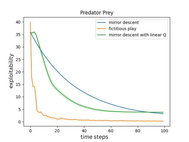
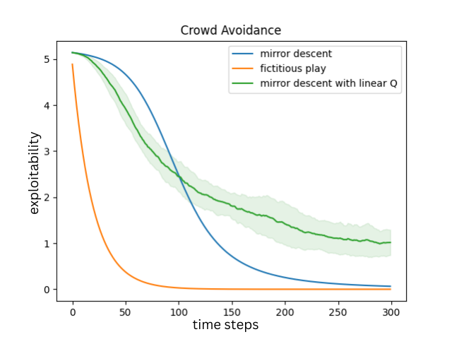
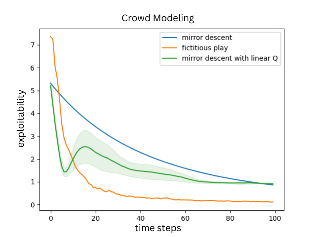
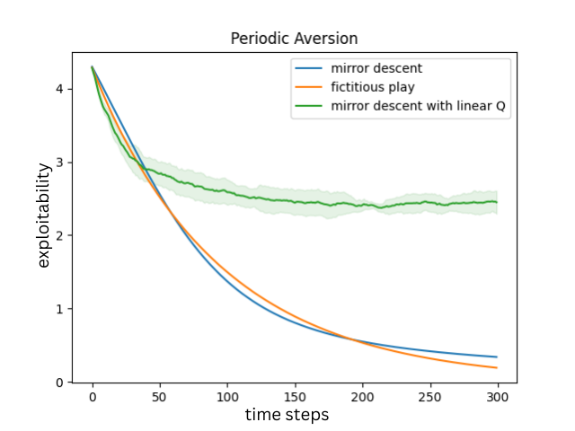
Figure 1: Experimental results for the mean field games described.

7 Conclusion

In this work, we present the first last-iterate convergence rate for monotone GMFGs with a mirror-descent algorithm. In tabular monotone GMFGs and under bandit feedback, we obtain a $O(T^{-1/4})$ last-iterate convergence rate. Under access to the exact cost and transition functions, we improved the rate to $O(T^{-1})$. In linear GMFGs, we achieve a last-iterate convergence rate of $O(T^{-1/5})$ under bandit feedback. Our study improves the understanding of mean-field games and the commonly used algorithms by providing insights both theoretically and numerically.

Appendix A Proof of Theorem 5.1

Proof.

By the update rule, we have

$$D_{\mathrm{KL}}\left(\pi^{\ast,\alpha}(\cdot\mid s_{h}^{\alpha}),\pi_{t+1,h}^{\alpha}(\cdot\mid s_{h}^{\alpha})\right)$$

$$=\ D_{\mathrm{KL}}\left(\pi^{\ast,\alpha}(\cdot\mid s_{h}^{\alpha}),\pi_{t,h}^{\alpha}(\cdot\mid s_{h}^{\alpha})\right)-D_{\mathrm{KL}}\left(\pi_{t+1,h}^{\alpha}(\cdot\mid s_{h}^{\alpha}),\pi_{t,h}^{\alpha}(\cdot\mid s_{h}^{\alpha})\right)$$

$$\ +\eta_{t}\left\langle\pi^{\ast,\alpha}(\cdot\mid s_{h}^{\alpha})-\pi_{t+1,h}^{\alpha}(\cdot\mid s_{h}^{\alpha}),Q^{\lambda,\alpha}_{h}\left(s_{h}^{\alpha},\cdot,\pi^{\beta}_{t},\mu^{\mathcal{I}}\right)+\lambda\log(\pi_{t,h}^{\alpha}(\cdot\mid s_{h}^{\alpha}))\right\rangle$$

$$=\ D_{\mathrm{KL}}\left(\pi^{\ast,\alpha}(\cdot\mid s_{h}^{\alpha}),\pi_{t,h}^{\alpha}(\cdot\mid s_{h}^{\alpha})\right)-D_{\mathrm{KL}}\left(\pi_{t+1,h}^{\alpha}(\cdot\mid s_{h}^{\alpha}),\pi_{t,h}^{\alpha}(\cdot\mid s_{h}^{\alpha})\right)$$

$$\ +\eta_{t}\left\langle\pi^{\ast,\alpha}(\cdot\mid s_{h}^{\alpha})-\pi_{t,h}^{\alpha}(\cdot\mid s_{h}^{\alpha}),Q^{\lambda,\alpha}_{h}\left(s_{h}^{\alpha},\cdot,\pi^{\beta}_{t},\mu^{\mathcal{I}}\right)+\lambda\log(\pi_{t,h}^{\alpha}(\cdot\mid s_{h}^{\alpha}))\right\rangle$$

$$\ +\eta_{t}\left\langle\pi_{t,h}^{\alpha}(\cdot\mid s_{h}^{\alpha})-\pi_{t+1,h}^{\alpha}(\cdot\mid s_{h}^{\alpha}),Q^{\lambda,\alpha}_{h}\left(s_{h}^{\alpha},\cdot,\pi^{\beta}_{t},\mu^{\mathcal{I}}\right)+\lambda\log(\pi_{t,h}^{\alpha}(\cdot\mid s_{h}^{\alpha}))\right\rangle$$

$$\leq\ D_{\mathrm{KL}}\left(\pi^{\ast,\alpha}(\cdot\mid s_{h}^{\alpha}),\pi_{t,h}^{\alpha}(\cdot\mid s_{h}^{\alpha})\right)-D_{\mathrm{KL}}\left(\pi_{t+1,h}^{\alpha}(\cdot\mid s_{h}^{\alpha}),\pi_{t,h}^{\alpha}(\cdot\mid s_{h}^{\alpha})\right)$$

$$\ +\eta_{t}\left\|\pi_{t+1,h}^{\alpha}(\cdot\mid s_{h}^{\alpha})-\pi_{t,h}^{\alpha}(\cdot\mid s_{h}^{\alpha})\right\|_{1}\left\|Q^{\lambda,\alpha}_{h}\left(s_{h}^{\alpha},\cdot,\pi^{\beta}_{t},\mu^{\mathcal{I}}\right)\right\|_{\infty}$$

$$\ +\eta_{t}\left\langle\pi^{\ast,\alpha}(\cdot\mid s_{h}^{\alpha})-\pi_{t,h}^{\alpha}(\cdot\mid s_{h}^{\alpha}),Q^{\lambda,\alpha}_{h}\left(s_{h}^{\alpha},\cdot,\pi^{\beta}_{t},\mu^{\mathcal{I}}\right)+\lambda\log(\pi_{t,h}^{\alpha}(\cdot\mid s_{h}^{\alpha}))\right\rangle$$

$$\leq\ D_{\mathrm{KL}}\left(\pi^{\ast,\alpha}(\cdot\mid s_{h}^{\alpha}),\pi_{t,h}^{\alpha}(\cdot\mid s_{h}^{\alpha})\right)-D_{\mathrm{KL}}\left(\pi_{t+1,h}^{\alpha}(\cdot\mid s_{h}^{\alpha}),\pi_{t,h}^{\alpha}(\cdot\mid s_{h}^{\alpha})\right)+\eta_{t}H\sqrt{2D_{\mathrm{KL}}\left(\pi_{t+1,h}^{\alpha}(\cdot\mid s_{h}^{\alpha}),\pi_{t,h}^{\alpha}(\cdot\mid s_{h}^{\alpha})\right)}$$

$$\ +\eta_{t}\left\langle\pi^{\ast,\alpha}(\cdot\mid s_{h}^{\alpha})-\pi_{t,h}^{\alpha}(\cdot\mid s_{h}^{\alpha}),Q^{\lambda,\alpha}_{h}\left(s_{h}^{\alpha},\cdot,\pi^{\beta}_{t},\mu^{\mathcal{I}}\right)+\lambda\log(\pi_{t,h}^{\alpha}(\cdot\mid s_{h}^{\alpha}))\right\rangle$$

$$\leq\ D_{\mathrm{KL}}\left(\pi^{\ast,\alpha}(\cdot\mid s_{h}^{\alpha}),\pi_{t,h}^{\alpha}(\cdot\mid s_{h}^{\alpha})\right)+\frac{\eta_{t}^{2}H^{2}}{2}+\eta_{t}\left\langle\pi^{\ast,\alpha}(\cdot\mid s_{h}^{\alpha})-\pi_{t,h}^{\alpha}(\cdot\mid s_{h}^{\alpha}),Q^{\lambda,\alpha}_{h}\left(s_{h}^{\alpha},\cdot,\pi^{\beta}_{t},\mu^{\mathcal{I}}\right)+\lambda\log(\pi_{t,h}^{\alpha}(\cdot\mid s_{h}^{\alpha}))\right\rangle\,.$$

Notice that $V^{\lambda,\alpha}_{h}\left(s_{h}^{\alpha},\pi^{\alpha},\mu^{\mathcal{I}}_{t}\right)=\left\langle Q^{\lambda,\alpha}_{h}\left(s_{h}^{\alpha},\cdot,\pi^{\alpha},\mu^{\mathcal{I}}_{t}\right)+\lambda\log(\pi^{\alpha}(\cdot\mid s_{h})),\pi^{\alpha}(\cdot\mid s_{h})\right\rangle$. By the definition of the value function and the performance difference lemma, we have

$$V^{\lambda,\alpha}_{1}\left(s^{\alpha},\pi^{\ast,\alpha},\mu^{\mathcal{I}}_{t}\right)-V^{\lambda,\alpha}_{1}\left(s^{\alpha},\pi^{\alpha},\mu^{\mathcal{I}}_{t}\right)$$

$$=\ \mathbb{E}_{\pi^{\ast,\alpha},\mu^{\mathcal{I}}_{t}}\left[\sum^{H}_{h=1}c_{h}(s_{h}^{\alpha},a_{h}^{\alpha},z_{h}^{\alpha})+\lambda\log(\pi_{h}^{\ast,\alpha}(\cdot\mid s_{h}^{\alpha}))\mid s_{1}=s\right]-V^{\lambda,\alpha}_{1}\left(s^{\alpha},\pi^{\alpha},\mu^{\mathcal{I}}_{t}\right)$$

$$=\ \mathbb{E}_{\pi^{\ast,\alpha},\mu^{\mathcal{I}}_{t}}\left[\sum^{H}_{h=1}c_{h}(s_{h}^{\alpha},a_{h}^{\alpha},z_{h}^{\alpha})+\lambda\log(\pi_{h}^{\ast,\alpha}(\cdot\mid s_{h}^{\alpha}))+V^{\lambda,\alpha}_{h}\left(s_{h}^{\alpha},\pi^{\alpha},\mu^{\mathcal{I}}_{t}\right)-V^{\lambda,\alpha}_{h}\left(s_{h}^{\alpha},\pi^{\alpha},\mu^{\mathcal{I}}_{t}\right)\mid s_{1}^{\alpha}=s^{\alpha}\right]$$

$$\ -V^{\lambda,\alpha}_{1}\left(s^{\alpha},\pi^{\alpha},\mu^{\mathcal{I}}_{t}\right)$$

$$=\ \mathbb{E}_{\pi^{\ast,\alpha},\mu^{\mathcal{I}}_{t}}\left[\sum^{H}_{h=1}c_{h}(s_{h}^{\alpha},a_{h}^{\alpha},z_{h}^{\alpha})+V^{\lambda,\alpha}_{h+1}\left(s_{h+1}^{\alpha},\pi^{\alpha},\mu^{\mathcal{I}}_{t}\right)+\lambda\log(\pi_{h}^{\ast,\alpha}(\cdot\mid s_{h}^{\alpha}))-V^{\lambda,\alpha}_{h}\left(s_{h}^{\alpha},\pi^{\alpha},\mu^{\mathcal{I}}_{t}\right)\mid s_{1}^{\alpha}=s^{\alpha}\right]$$

$$=\ \mathbb{E}_{\pi^{\ast,\alpha},\mu^{\mathcal{I}}_{t}}\left[\sum^{H}_{h=1}\left\langle Q^{\lambda,\alpha}_{h}\left(s_{h}^{\alpha},\cdot,\pi^{\alpha},\mu^{\mathcal{I}}_{t}\right)+\lambda\log(\pi_{h}^{\ast,\alpha}(\cdot\mid s_{h}^{\alpha})),\pi_{h}^{\ast,\alpha}(\cdot\mid s_{h}^{\alpha})\right\rangle-V^{\lambda,\alpha}_{h}\left(s_{h}^{\alpha},\pi^{\alpha},\mu^{\mathcal{I}}_{t}\right)\mid s_{1}^{\alpha}=s^{\alpha}\right]$$

$$=\ \mathbb{E}_{\pi^{\ast,\alpha},\mu^{\mathcal{I}}_{t}}\left[\sum^{H}_{h=1}\left\langle Q^{\lambda,\alpha}_{h}\left(s_{h}^{\alpha},\cdot,\pi^{\alpha},\mu^{\mathcal{I}}_{t}\right),\pi_{h}^{\ast,\alpha}(\cdot\mid s_{h}^{\alpha})-\pi_{h}^{\alpha}(\cdot\mid s_{h}^{\alpha})\right\rangle\mid s_{1}^{\alpha}=s^{\alpha}\right]$$

$$\ +\lambda\mathbb{E}_{\pi^{\ast,\alpha},\mu^{\mathcal{I}}_{t}}\left[\sum^{H}_{h=1}\left\langle\log\left(\pi_{h}^{\ast,\alpha}(\cdot\mid s_{h}^{\alpha})\right),\pi_{h}^{\ast,\alpha}(\cdot\mid s_{h}^{\alpha})\right\rangle-\left\langle\log(\pi^{\alpha}(\cdot\mid s_{h}^{\alpha})),\pi^{\alpha}(\cdot\mid s_{h}^{\alpha})\right\rangle\mid s_{1}^{\alpha}=s^{\alpha}\right]$$

$$=\ \mathbb{E}_{\pi^{\ast,\alpha},\mu^{\mathcal{I}}_{t}}\left[\sum^{H}_{h=1}\left\langle Q^{\lambda,\alpha}_{h}\left(s_{h}^{\alpha},\cdot,\pi^{\alpha},\mu^{\mathcal{I}}_{t}\right)+\lambda\log(\pi^{\alpha}(\cdot\mid s_{h}^{\alpha})),\pi_{h}^{\ast,\alpha}(\cdot\mid s_{h}^{\alpha})-\pi_{h}^{\alpha}(\cdot\mid s_{h}^{\alpha})\right\rangle\mid s_{1}^{\alpha}=s^{\alpha}\right]$$

$$\ +\lambda\mathbb{E}_{\pi^{\ast,\alpha},\mu^{\mathcal{I}}_{t}}\left[\sum^{H}_{h=1}D_{\mathrm{KL}}\left(\pi^{\ast,\alpha}(\cdot\mid s_{h}^{\alpha}),\pi_{h}^{\alpha}(\cdot\mid s_{h}^{\alpha})\right)\mid s_{1}^{\alpha}=s^{\alpha}\right]\,.$$

Summing over $H$ and taking integral over $\alpha$, we therefore have

$$\int_{\mathcal{I}}\sum^{H}_{h=1}\mathbb{E}_{\mu^{\ast,\alpha}_{h}}\left[D_{\mathrm{KL}}\left(\pi^{\ast,\alpha}(\cdot\mid s_{h}^{\alpha}),\pi_{t+1,h}^{\alpha}(\cdot\mid s_{h}^{\alpha})\right)\right]d\nu(\alpha)$$

$$\leq\ \left(1-\eta_{t}\lambda\right)\int_{\mathcal{I}}\sum^{H}_{h=1}\mathbb{E}_{\mu^{\ast,\alpha}_{h}}\left[D_{\mathrm{KL}}\left(\pi^{\ast,\alpha}(\cdot\mid s_{h}^{\alpha}),\pi_{t,h}^{\alpha}(\cdot\mid s_{h}^{\alpha})\right)\right]d\nu(\alpha)+\eta_{t}^{2}H^{3}$$

$$\ +\eta_{t}\int_{\mathcal{I}}\left(J^{\lambda,\alpha}(\pi^{\ast,\alpha},\mu_{t}^{\mathcal{I}})-J^{\lambda,\alpha}(\pi^{\alpha},\mu_{t}^{\mathcal{I}})\right)d\nu(\alpha)$$

$$\leq\ \left(1-\eta_{t}\lambda\right)\int_{\mathcal{I}}\sum^{H}_{h=1}\mathbb{E}_{\mu^{\ast,\alpha}_{h}}\left[D_{\mathrm{KL}}\left(\pi^{\ast,\alpha}(\cdot\mid s_{h}^{\alpha}),\pi_{t,h}^{\alpha}(\cdot\mid s_{h}^{\alpha})\right)\right]d\nu(\alpha)+\eta_{t}^{2}H^{3}\,,$$

as by proposition 3.1, $\int_{\mathcal{I}}J^{\lambda,\alpha}(\pi^{\ast,\alpha},\mu_{t}^{\mathcal{I}})-J^{\lambda,\alpha}(\pi^{\alpha},\mu_{t}^{\mathcal{I}})d\nu(\alpha)\leq\int_{\mathcal{I}}J^{\lambda,\alpha}(\pi^{\ast,\alpha},\mu_{t}^{\ast,\mathcal{I}})-J^{\lambda,\alpha}(\pi^{\alpha},\mu_{t}^{\ast,\mathcal{I}})d\nu(\alpha)\leq 0$, by optimality.

Thus, let $\eta_{t}=t^{-1}$, we have

$$D\left(\pi^{\mathcal{I}}_{t+1}\right)\leq\ (1-\eta_{t}\lambda)D\left(\pi^{\mathcal{I}}_{t}\right)+\eta_{t}^{2}H^{3}\leq\frac{H^{3}}{\lambda t}\,.$$

∎

Appendix B Proof of Theorem 5.2

Proof.

By the update rule, we have

$$D_{\mathrm{KL}}\left(\pi^{\ast,\alpha}(\cdot\mid s_{h}^{\alpha}),\pi_{t+1,h}^{\alpha}(\cdot\mid s_{h}^{\alpha})\right)$$

$$=\ D_{\mathrm{KL}}\left(\pi^{\ast,\alpha}(\cdot\mid s_{h}^{\alpha}),\pi_{t,h}^{\alpha}(\cdot\mid s_{h}^{\alpha})\right)-D_{\mathrm{KL}}\left(\pi_{t+1,h}^{\alpha}(\cdot\mid s_{h}^{\alpha}),\pi_{t,h}^{\alpha}(\cdot\mid s_{h}^{\alpha})\right)$$

$$\ +\eta_{t}\left\langle\pi^{\ast,\alpha}(\cdot\mid s_{h}^{\alpha})-\pi_{t+1,h}^{\alpha}(\cdot\mid s_{h}^{\alpha}),\hat{g}_{t,h}(s_{h}^{\alpha},\cdot)+\lambda\log(\pi_{t,h}^{\alpha}(\cdot\mid s_{h}^{\alpha}))\right\rangle$$

$$=\ D_{\mathrm{KL}}\left(\pi^{\ast,\alpha}(\cdot\mid s_{h}^{\alpha}),\pi_{t,h}^{\alpha}(\cdot\mid s_{h}^{\alpha})\right)-D_{\mathrm{KL}}\left(\pi_{t+1,h}^{\alpha}(\cdot\mid s_{h}^{\alpha}),\pi_{t,h}^{\alpha}(\cdot\mid s_{h}^{\alpha})\right)$$

$$\ +\eta_{t}\left\langle\pi^{\ast,\alpha}(\cdot\mid s_{h}^{\alpha})-\pi_{t,h}^{\alpha}(\cdot\mid s_{h}^{\alpha}),\hat{g}_{t,h}(s_{h}^{\alpha},\cdot)+\lambda\log(\pi_{t,h}^{\alpha}(\cdot\mid s_{h}^{\alpha}))\right\rangle$$

$$\ +\eta_{t}\left\langle\pi_{t,h}^{\alpha}(\cdot\mid s_{h}^{\alpha})-\pi_{t+1,h}^{\alpha}(\cdot\mid s_{h}^{\alpha}),\hat{g}_{t,h}(s_{h}^{\alpha},\cdot)+\lambda\log(\pi_{t,h}^{\alpha}(\cdot\mid s_{h}^{\alpha}))\right\rangle$$

$$\leq\ D_{\mathrm{KL}}\left(\pi^{\ast,\alpha}(\cdot\mid s_{h}^{\alpha}),\pi_{t,h}^{\alpha}(\cdot\mid s_{h}^{\alpha})\right)-D_{\mathrm{KL}}\left(\pi_{t+1,h}^{\alpha}(\cdot\mid s_{h}^{\alpha}),\pi_{t,h}^{\alpha}(\cdot\mid s_{h}^{\alpha})\right)$$

$$\ +\eta_{t}\left\|\pi_{t+1,h}^{\alpha}(\cdot\mid s_{h}^{\alpha})-\pi_{t,h}^{\alpha}(\cdot\mid s_{h}^{\alpha})\right\|_{1}\left\|\hat{g}_{t,h}(s_{h}^{\alpha},\cdot)\right\|_{\infty}$$

$$\ +\eta_{t}\left\langle\pi^{\ast,\alpha}(\cdot\mid s_{h}^{\alpha})-\pi_{t,h}^{\alpha}(\cdot\mid s_{h}^{\alpha}),\hat{g}_{t,h}(s_{h}^{\alpha},\cdot)+\lambda\log(\pi_{t,h}^{\alpha}(\cdot\mid s_{h}^{\alpha}))\right\rangle$$

$$\leq\ D_{\mathrm{KL}}\left(\pi^{\ast,\alpha}(\cdot\mid s_{h}^{\alpha}),\pi_{t,h}^{\alpha}(\cdot\mid s_{h}^{\alpha})\right)-D_{\mathrm{KL}}\left(\pi_{t+1,h}^{\alpha}(\cdot\mid s_{h}^{\alpha}),\pi_{t,h}^{\alpha}(\cdot\mid s_{h}^{\alpha})\right)+\frac{\eta_{t}H}{\gamma_{t}}\sqrt{2D_{\mathrm{KL}}\left(\pi_{t+1,h}^{\alpha}(\cdot\mid s_{h}^{\alpha}),\pi_{t,h}^{\alpha}(\cdot\mid s_{h}^{\alpha})\right)}$$

$$\ +\eta_{t}\left\langle\pi^{\ast,\alpha}(\cdot\mid s_{h}^{\alpha})-\pi_{t,h}^{\alpha}(\cdot\mid s_{h}^{\alpha}),\hat{g}_{t,h}(s_{h}^{\alpha},\cdot)+\lambda\log(\pi_{t,h}^{\alpha}(\cdot\mid s_{h}^{\alpha}))\right\rangle$$

$$\leq\ D_{\mathrm{KL}}\left(\pi^{\ast,\alpha}(\cdot\mid s_{h}^{\alpha}),\pi_{t,h}^{\alpha}(\cdot\mid s_{h}^{\alpha})\right)+\frac{\eta_{t}^{2}H^{2}}{2\gamma_{t}^{2}}+\eta_{t}\left\langle\pi^{\ast,\alpha}(\cdot\mid s_{h}^{\alpha})-\pi_{t,h}^{\alpha}(\cdot\mid s_{h}^{\alpha}),Q^{\lambda,\alpha}_{h}\left(s_{h}^{\alpha},\cdot,\pi^{\beta}_{t},\mu^{\mathcal{I}}\right)+\lambda\log(\pi_{t,h}^{\alpha}(\cdot\mid s_{h}^{\alpha}))\right\rangle$$

$$\ +\eta_{t}\left\langle\pi^{\ast,\alpha}(\cdot\mid s_{h}^{\alpha})-\pi_{t,h}^{\alpha}(\cdot\mid s_{h}^{\alpha}),\hat{g}_{t,h}(s_{h}^{\alpha},\cdot)-Q^{\lambda,\alpha}_{h}\left(s_{h}^{\alpha},\cdot,\pi^{\beta}_{t},\mu^{\mathcal{I}}\right)\right\rangle\,.$$

For the last term,

$$\eta_{t}\left\langle\pi^{\ast,\alpha}(\cdot\mid s_{h}^{\alpha})-\pi_{t,h}^{\alpha}(\cdot\mid s_{h}^{\alpha}),\hat{g}_{t,h}(s_{h}^{\alpha},\cdot)-Q^{\lambda,\alpha}_{h}\left(s_{h}^{\alpha},\cdot,\pi^{\beta}_{t},\mu^{\mathcal{I}}\right)\right\rangle$$

$$=\ \eta_{t}\left\langle\pi^{\ast,\alpha}(\cdot\mid s_{h}^{\alpha})-\pi_{t,h}^{\alpha}(\cdot\mid s_{h}^{\alpha}),\frac{\mathbb{I}\{a_{h}=a\}\left(c_{h}+\hat{V}^{\lambda,\alpha}_{h+1}\left(s_{h+1}^{\alpha},\pi_{t}^{\alpha},\mu^{\mathcal{I}}\right)\right)}{\pi_{t,h}(s_{h})+\gamma_{t}}-\frac{\mathbb{I}\{a_{h}=a\}\left(c_{h}+V^{\lambda,\alpha}_{h+1}\left(s_{h+1}^{\alpha},\pi_{t}^{\alpha},\mu^{\mathcal{I}}\right)\right)}{\pi_{t,h}(s_{h})+\gamma_{t}}\right\rangle$$

$$+ \ \eta_{t}\left\langle\pi^{\ast,\alpha}(\cdot\mid s_{h}^{\alpha})-\pi_{t,h}^{\alpha}(\cdot\mid s_{h}^{\alpha}),\frac{\mathbb{I}\{a_{h}=a\}\left(c_{h}+V^{\lambda,\alpha}_{h+1}\left(s_{h+1}^{\alpha},\pi_{t}^{\alpha},\mu^{\mathcal{I}}\right)\right)}{\pi_{t,h}(s_{h})+\gamma_{t}}-\left(c_{h}+\mathbb{E}_{\pi^{\alpha}}\left[V^{\lambda,\alpha}_{h+1}\left(s_{h+1}^{\alpha},\pi^{\alpha},\mu^{\mathcal{I}}\right)\right]\right)\right\rangle$$

$$\leq\ \frac{\eta_{t}}{\gamma_{t}}\left|\hat{V}^{\lambda,\alpha}_{h+1}\left(s_{h+1}^{\alpha},\pi_{t}^{\alpha},\mu^{\mathcal{I}}\right)-V^{\lambda,\alpha}_{h+1}\left(s_{h+1}^{\alpha},\pi_{t}^{\alpha},\mu^{\mathcal{I}}\right)\right|+\eta_{t}\epsilon_{t,h}+\eta_{t}\zeta_{t,h}\,.$$

where

$$\epsilon_{t,h}=\ \left\langle\pi^{\ast,\alpha}(\cdot\mid s_{h}^{\alpha}),\frac{\mathbb{I}\{a_{h}=a\}\left(c_{h}+V^{\lambda,\alpha}_{h+1}\left(s_{h+1}^{\alpha},\pi_{t}^{\alpha},\mu^{\mathcal{I}}\right)\right)}{\pi_{t,h}(s_{h})+\gamma_{t}}-\left(c_{h}+\mathbb{E}_{\pi^{\alpha}}\left[V^{\lambda,\alpha}_{h+1}\left(s_{h+1}^{\alpha},\pi^{\alpha},\mu^{\mathcal{I}}\right)\right]\right)\right\rangle$$

$$\zeta_{t,h}=\ \left\langle\pi_{t,h}^{\alpha}(\cdot\mid s_{h}^{\alpha}),\left(c_{h}+\mathbb{E}_{\pi^{\alpha}}\left[V^{\lambda,\alpha}_{h+1}\left(s_{h+1}^{\alpha},\pi^{\alpha},\mu^{\mathcal{I}}\right)\right]\right)-\frac{\mathbb{I}\{a_{h}=a\}\left(c_{h}+V^{\lambda,\alpha}_{h+1}\left(s_{h+1}^{\alpha},\pi_{t}^{\alpha},\mu^{\mathcal{I}}\right)\right)}{\pi_{t,h}(s_{h})+\gamma_{t}}\right\rangle\,.$$

Choose $\beta_{t}=\frac{H+1}{H+t}$, by Lemma B.1, we have $\left(\hat{V}^{\lambda,\alpha}_{h+1}\left(s_{h+1}^{\alpha},\pi_{t}^{\alpha},\mu^{\mathcal{I}}\right)-V^{\lambda,\alpha}_{h+1}\left(s_{h+1}^{\alpha},\pi_{t}^{\alpha},\mu^{\mathcal{I}}\right)\right)\leq O\left(\sqrt{\frac{H^{3}\log(HSAT/\delta)}{t}}\right)$.

Define $\omega_{t}^{k}=\prod^{t}_{j=k+1}\left(1-\eta_{j}\lambda\right)$, and $\iota=\log(HSAT/\delta)$. Similar to the proof of the exact gradient case, using the monotonicity condition and summing over $H$ and set $\eta_{0}\lambda=1$, we therefore have

$$\sum^{H}_{h=1}\mathbb{E}_{\mu^{\ast,\alpha}_{h}}\left[D_{\mathrm{KL}}\left(\pi^{\ast,\alpha}(\cdot\mid s_{h}^{\alpha}),\pi_{t+1,h}^{\alpha}(\cdot\mid s_{h}^{\alpha})\right)\right]$$

$$\leq\ \left(1-\eta_{t}\lambda\right)\sum^{H}_{h=1}\mathbb{E}_{\mu^{\ast,\alpha}_{h}}\left[D_{\mathrm{KL}}\left(\pi^{\ast,\alpha}(\cdot\mid s_{h}^{\alpha}),\pi_{t,h}^{\alpha}(\cdot\mid s_{h}^{\alpha})\right)\right]+\sum^{H}_{h=1}\left(\epsilon_{t,h}+\zeta_{t,h}\right)+\frac{\eta_{t}^{2}H^{3}}{2\gamma_{t}^{2}}+\frac{\eta_{t}\sqrt{H^{3}\iota}}{\gamma_{t}\sqrt{t}}$$

$$=\ \sum^{H}_{h=1}\sum^{t}_{k=1}\eta_{k}\omega_{t}^{k}\left(\epsilon_{k,h}+\zeta_{k,h}\right)+\sum^{t}_{k=1}\omega_{t}^{k}\left(\frac{\eta_{k}^{2}H^{3}}{2\gamma_{k}^{2}}+\frac{\eta_{k}\sqrt{H^{3}\iota}}{\gamma_{t}\sqrt{t}}\right)$$

$$\leq\ O\left(A\sum^{t}_{k=1}\gamma_{k}\eta_{k}\omega_{t}^{k}+\sqrt{\log(A/\delta)\sum^{t}_{k=1}\eta_{k}^{2}(\omega_{t}^{k})^{2}}+\max_{k\in[t]}\frac{\eta_{k}\omega_{t}^{k}\log(1/\delta)}{\gamma_{k}}+\sum^{t}_{k=1}\omega_{t}^{k}\left(\frac{\eta_{k}^{2}H^{3}}{2\gamma_{k}^{2}}+\frac{\eta_{k}\sqrt{H^{3}\iota}}{\gamma_{k}\sqrt{t}}\right)\right)\,,$$

where the last inequality is by Lemma C.1 and Lemma C.2.

Take $\eta_{k}=\frac{1}{\lambda k^{c_{\eta}}}$, $\gamma_{k}=\frac{1}{k^{c_{\gamma}}}$, by Lemma C.3, we have

$$O\left(A\sum^{t}_{k=1}\gamma_{k}\eta_{k}\omega_{t}^{k}+\sqrt{\log(A/\delta)\sum^{t}_{k=1}\eta_{k}^{2}(\omega_{t}^{k})^{2}}\right)=\ O\left(\frac{A\log(t)}{t^{c_{\gamma}}}+\sqrt{\frac{\log(A/\delta)}{t^{2c_{\gamma}}}}\right)\,,$$

$$O\left(\sum^{t}_{k=1}\omega_{t}^{k}\left(\frac{\eta_{k}^{2}H^{3}}{2\gamma_{k}^{2}}+\frac{\eta_{k}\sqrt{H^{3}\iota}}{\sqrt{t}}\right)\right)=\ O\left(\frac{H^{3}}{t^{c_{\eta}-2c_{\gamma}}}+\frac{\sqrt{H^{3}\iota}}{t^{1/2-c_{\gamma}}}\right)\,.$$

By Lemma C.4, we have

$$O\left(\max_{k\in[t]}\frac{\eta_{k}\omega_{t}^{k}\log(1/\delta)}{\gamma_{t}}\right)=O\left(\frac{\log(1/\delta)}{t^{c_{\eta}-c_{\gamma}}}\right)$$

Take $c_{\eta}=3/4,c_{\gamma}=1/4$, and integrating over $\alpha\in[0,1]$, we therefore have

$$D\left(\pi^{\mathcal{I}}_{t+1}\right)\leq O\left(\frac{A\log(t)}{t^{3/4}}+\frac{\sqrt{\log(A/\delta)}}{t^{3/4}}+\frac{H^{3}}{t^{1/4}}+\frac{\sqrt{H^{3}\iota}}{t^{1/4}}+\frac{\log(1/\delta)}{t^{1/2}}\right)\,.$$

∎

Lemma B.1.

For any $h,t,\alpha$, take $\beta_{t}=\frac{H+1}{H+t}$, and we have

$$\left|\hat{V}^{\lambda,\alpha}_{h}\left(s_{h}^{\alpha},\pi_{t}^{\alpha},\mu^{\mathcal{I}}\right)-V^{\lambda,\alpha}_{h}\left(s_{h}^{\alpha},\pi_{t}^{\alpha},\mu^{\mathcal{I}}\right)\right|\leq O\left(\sqrt{\frac{H^{3}\log(HSAT/\delta)}{t}}\right)\,.$$

Proof.

Define an auxiliary sequence $\left\{\beta_{t}^{i}\right\}_{i=1}^{t}$ based on the learning rate.

$$\beta_{t}=\frac{H+1}{H+t},\quad\beta_{t}^{0}=\prod_{j=1}^{t}\left(1-\beta_{j}\right),\quad\beta_{t}^{i}=\beta_{i}\prod_{j=i+1}^{t}\left(1-\beta_{j}\right)\,.$$

Let $k$ denote the number of times $s$ is visited at step $h$ at the beginning of episode $t$, and suppose s was previously visited at episodes $t^{1},\ldots,t^{k}<t$ at the $h$-th step. Then by Lemma 11 of Jin et al., (2022), we can write

$$\hat{V}^{\lambda,\alpha}_{t,h}\left(s_{h}^{\alpha},\pi_{t}^{\alpha},\mu^{\mathcal{I}}\right)=\ \sum^{k}_{i=1}\beta_{k}^{i}\left(c_{h}(s_{h}^{\alpha},a_{h}^{\alpha,t^{i}})+\hat{V}^{\lambda,\alpha}_{t,h+1}\left(s^{t^{i}}_{h+1},\pi_{t^{i}}^{\alpha},\mu^{\mathcal{I}}\right)\right)\,.$$

We denote $\left(P_{h}V^{\lambda,\alpha}_{h+1}\left(\pi_{t^{i}}^{\alpha},\mu^{\mathcal{I}}\right)\right)(s,a)=\mathbb{E}_{\pi_{t^{i}}^{\alpha},s^{\prime}\sim P_{h}(\cdot\mid s,a)}V^{\lambda,\alpha}_{h+1}\left(s^{\prime},\pi_{t^{i}}^{\alpha},\mu^{\mathcal{I}}\right)$. We also let $\hat{P}_{h}^{t}$ to denote the actual state tradition experienced under $\pi_{t}^{\alpha},\mu^{\mathcal{I}}$ at episode $t$. By the Bellman equation, and using the fact that $\sum^{t}_{i=0}\beta_{t}^{i}=1$, we have

$$V^{\lambda,\alpha}_{h}\left(s_{h}^{\alpha},\pi_{t}^{\alpha},\mu^{\mathcal{I}}\right)$$

$$=\ \beta_{k}^{0}V^{\lambda,\alpha}_{h}\left(s_{h}^{\alpha},\pi_{t}^{\alpha},\mu^{\mathcal{I}}\right)+\sum^{k}_{i=1}\beta_{k}^{i}\mathbb{E}_{\pi_{t^{i}}^{\alpha}}\left[\left(c_{h}(s_{h}^{\alpha},a^{\alpha})+\left(P_{h}V^{\lambda,\alpha}_{h+1}\left(\pi_{t^{i}}^{\alpha},\mu^{\mathcal{I}}\right)\right)(s_{h}^{\alpha},a^{\alpha})\right)\right]$$

$$=\ \beta_{k}^{0}V^{\lambda,\alpha}_{h}\left(s_{h}^{\alpha},\pi_{t}^{\alpha},\mu^{\mathcal{I}}\right)+\sum^{k}_{i=1}\beta_{k}^{i}\mathbb{E}_{\pi_{t^{i}}^{\alpha}}\left[\left(c_{h}(s_{h}^{\alpha},a^{\alpha})+\left(\left(P_{h}-\hat{P}_{h}^{t_{i}}\right)V^{\lambda,\alpha}_{h+1}\left(\pi_{t^{i}}^{\alpha},\mu^{\mathcal{I}}\right)\right)(s_{h}^{\alpha},a^{\alpha})\right)\right]$$

$$\ -\beta_{k}^{i}V^{\lambda,\alpha}_{h+1}\left(s^{t^{i}}_{h+1},\pi_{t^{i}}^{\alpha},\mu^{\mathcal{I}}\right)$$

Therefore, we have the following recursion.

$$\hat{V}^{\lambda,\alpha}_{t,h}\left(s_{h}^{\alpha},\pi_{t}^{\alpha},\mu^{\mathcal{I}}\right)-V^{\lambda,\alpha}_{h}\left(s_{h}^{\alpha},\pi_{t}^{\alpha},\mu^{\mathcal{I}}\right)$$

$$\leq\ \sum^{k}_{i=1}\mathbb{E}_{\pi_{t^{i}}^{\alpha}}\left[\beta_{k}^{i}\left(\left(P_{h}-\hat{P}_{h}^{t_{i}}\right)V^{\lambda,\alpha}_{h+1}\left(\pi_{t^{i}}^{\alpha},\mu^{\mathcal{I}}\right)(s_{h}^{\alpha},a^{\alpha})\right)\right]+\beta_{k}^{i}\left(\hat{V}^{\lambda,\alpha}_{t^{i},h+1}\left(s^{t^{i}}_{h+1},\pi_{t^{i}}^{\alpha},\mu^{\mathcal{I}}\right)-V^{\lambda,\alpha}_{h+1}\left(s^{t^{i}}_{h+1},\pi_{t^{i}}^{\alpha},\mu^{\mathcal{I}}\right)\right)\,.$$

Applying Martingale concentration and using the property of the sequence $\beta_{k}^{i}$, we have

$$\hat{V}^{\lambda,\alpha}_{t,h}\left(s_{h}^{\alpha},\pi_{t}^{\alpha},\mu^{\mathcal{I}}\right)-V^{\lambda,\alpha}_{h}\left(s_{h}^{\alpha},\pi_{t}^{\alpha},\mu^{\mathcal{I}}\right)$$

$$\leq\ O\left(\sqrt{\frac{H^{3}\log(HSAT/\delta)}{t}}\right)+\sum^{k}_{i=1}\beta_{k}^{i}\left(\hat{V}^{\lambda,\alpha}_{t^{i},h+1}\left(s^{t^{i}}_{h+1},\pi_{t^{i}}^{\alpha},\mu^{\mathcal{I}}\right)-V^{\lambda,\alpha}_{h+1}\left(s^{t^{i}}_{h+1},\pi_{t^{i}}^{\alpha},\mu^{\mathcal{I}}\right)\right)\,.$$

We now upper bound this by induction. Suppose for $\tau=t^{i}$, $i=1,\ldots,k$, $\forall h\in[H]$

$$\hat{V}^{\lambda,\alpha}_{\tau,h}\left(s_{h}^{\alpha},\pi_{t}^{\alpha},\mu^{\mathcal{I}}\right)-V^{\lambda,\alpha}_{h}\left(s_{h}^{\alpha},\pi_{t}^{\alpha},\mu^{\mathcal{I}}\right)\leq O\left(\sqrt{\frac{H^{3}\log(HSAT/\delta)}{t}}\right)\,.$$

For $t=1$, the base case holds trivially. Then we consider $\hat{V}^{\lambda,\alpha}_{t,h}\left(s_{h}^{\alpha},\pi_{t}^{\alpha},\mu^{\mathcal{I}}\right)-V^{\lambda,\alpha}_{h}\left(s_{h}^{\alpha},\pi_{t}^{\alpha},\mu^{\mathcal{I}}\right)$, and notice that $t$ is the next update after time step $k$,

$$\sum^{k}_{i=1}\beta_{k}^{i}\left(\hat{V}^{\lambda,\alpha}_{t,h+1}\left(s^{t^{i}}_{h+1},\pi_{t^{i}}^{\alpha},\mu^{\mathcal{I}}\right)-V^{\lambda,\alpha}_{h+1}\left(s^{t^{i}}_{h+1},\pi_{t^{i}}^{\alpha},\mu^{\mathcal{I}}\right)\right)$$

$$\leq\ \sum^{k}_{i=1}O\left(\frac{2}{t}\cdot\sqrt{\frac{H^{3}\log(HSAT/\delta)}{t}}\right)\leq O\left(\sqrt{\frac{H^{3}\log(HSAT/\delta)}{t}}\right)\,.$$

where the first inequality is by Lemma 4.1 of Jin et al., (2018), $\max_{i\in[t]}\beta_{t}^{i}\leq\frac{2}{t}$, and the second inequality is due to $k\leq t$.

Hence, we have the claimed result.

∎

Appendix C Auxiliary lemmas for gradient estimation

Let $\mathbb{I}\{a_{h}=a\}$ be a one-hot vector where it is one at $a_{h}$. Suppose one run OMD with estimated gradient $\hat{g}_{t}$ to obtain $\pi_{t}$, where $\hat{g}_{t}(a)=\frac{\sigma_{t}\mathbb{I}\{a_{t}=a\}}{\pi_{t}(a)+\gamma_{t}}$, $\mathbb{E}[\mathbb{I}\{a_{t}=a\}\mid\mathcal{F}_{t-1}]=\pi_{t}(a)$, $\mathbb{E}[\sigma_{t}\mid\mathcal{F}_{t-1}]=g_{t}$, and $\mathcal{F}_{t-1}$ is the history generated up to time $t$. Here we let $\pi^{\ast}_{t}$ be the optimality policy, which is independent of $g_{t},\hat{g}_{t}$.

Lemma C.1 (Lemma 20 of Bai et al., (2020)).

Let $c_{1},c_{2},\ldots,c_{t}$ be fixed positive numbers. Then with probability at least $1-\delta$,

$$\sum_{i=1}^{t}c_{i}\left\langle\pi_{i},g_{i}-\hat{g}_{i}\right\rangle=\mathcal{O}\left(A\sum_{i=1}^{t}\gamma_{i}c_{i}+\sqrt{\ln(A/\delta)\sum_{i=1}^{t}c_{i}^{2}}\right)\,.$$

Lemma C.2 (Lemma 10 of Cai et al., (2023), Lemma 18 of Bai et al., (2020)).

Let $c_{1},c_{2},\ldots,c_{t}$ be fixed positive numbers. Then for any sequence $\pi_{1}^{\star},\ldots,\pi_{t}^{\star}\in\Delta_{A}$ such that $\pi_{i}^{\star}$ is $\mathcal{F}_{i-1}$-measurable, with probability at least $1-\delta$,

$$\sum_{i=1}^{t}c_{i}\left\langle\pi_{i}^{\star},\widehat{g}_{i}-g_{i}\right\rangle=\mathcal{O}\left(\max_{i\leq t}\frac{c_{i}\ln(1/\delta)}{\gamma_{t}}\right)\,.$$

Lemma C.3 (Lemma 4 of Cai et al., (2023)).

Let $0<h<1,0\leq k\leq 2$, and let $t\geq\left(\frac{24}{1-h}\ln\frac{12}{1-h}\right)^{\frac{1}{1-h}}$. Then

$$\sum_{i=1}^{t}\left(i^{-k}\prod_{j=i+1}^{t}\left(1-j^{-h}\right)\right)\leq 9\ln(t)t^{-k+h}\,.$$

Lemma C.4 (Lemma 4 of Cai et al., (2023)).

Let $0<h<1,0\leq k\leq 2$, and let $t\geq\left(\frac{24}{1-h}\ln\frac{12}{1-h}\right)^{\frac{1}{1-h}}$. Then

$$\max_{1\leq i\leq t}\left(i^{-k}\prod_{j=i+1}^{t}\left(1-j^{-h}\right)\right)\leq 4t^{-k}\,.$$

Appendix D Proof of Theorem 5.3

Proof.

Similar to Theorem 5.1, we have

$$D_{\mathrm{KL}}\left(\pi^{\ast,\alpha}(\cdot\mid s_{h}^{\alpha}),\pi_{t+1,h}^{\alpha}(\cdot\mid s_{h}^{\alpha})\right)$$

$$\leq\ D_{\mathrm{KL}}\left(\pi^{\ast,\alpha}(\cdot\mid s_{h}^{\alpha}),\pi_{t,h}^{\alpha}(\cdot\mid s_{h}^{\alpha})\right)+\frac{\eta_{t}^{2}H^{2}}{2\gamma_{t}^{2}}+\eta_{t}\left\langle\pi^{\ast,\alpha}(\cdot\mid s_{h}^{\alpha})-\pi_{t,h}^{\alpha}(\cdot\mid s_{h}^{\alpha}),Q^{\lambda,\alpha}_{h}\left(s_{h}^{\alpha},\cdot,\pi^{\beta}_{t},\mu^{\mathcal{I}}\right)+\lambda\log(\pi_{t,h}^{\alpha}(\cdot\mid s_{h}^{\alpha}))\right\rangle$$

$$\ +\eta_{t}\left\langle\pi^{\ast,\alpha}(\cdot\mid s_{h}^{\alpha})-\pi_{t,h}^{\alpha}(\cdot\mid s_{h}^{\alpha}),\hat{g}_{t,h}(s_{h}^{\alpha},\cdot)-Q^{\lambda,\alpha}_{h}\left(s_{h}^{\alpha},\cdot,\pi^{\beta}_{t},\mu^{\mathcal{I}}\right)\right\rangle\,.$$

For the last term,

$$\eta_{t}\left\langle\pi^{\ast,\alpha}(\cdot\mid s_{h}^{\alpha})-\pi_{t,h}^{\alpha}(\cdot\mid s_{h}^{\alpha}),\hat{g}_{t,h}(s_{h}^{\alpha},\cdot)-Q^{\lambda,\alpha}_{h}\left(s_{h}^{\alpha},\cdot,\pi^{\beta}_{t},\mu^{\mathcal{I}}\right)\right\rangle$$

$$=\ \eta_{t}\left\langle\pi^{\ast,\alpha}(\cdot\mid s_{h}^{\alpha})-\pi_{t,h}^{\alpha}(\cdot\mid s_{h}^{\alpha}),\frac{\mathbb{I}\{a_{h}=a\}\hat{Q}^{\lambda,\alpha}_{t,h}\left(s^{\alpha}_{h},a^{\alpha}_{h},\pi^{\alpha}_{t},\mu^{\mathcal{I}}\right)}{\pi_{t,h}(s_{h})+\gamma_{t}}-\frac{\mathbb{I}\{a_{h}=a\}Q^{\lambda,\alpha}_{t,h}\left(s^{\alpha}_{h},a^{\alpha}_{h},\pi^{\alpha}_{t},\mu^{\mathcal{I}}\right)}{\pi_{t,h}(s_{h})+\gamma_{t}}\right\rangle$$

$$+ \ \eta_{t}\left\langle\pi^{\ast,\alpha}(\cdot\mid s_{h}^{\alpha})-\pi_{t,h}^{\alpha}(\cdot\mid s_{h}^{\alpha}),\frac{\mathbb{I}\{a_{h}=a\}Q^{\lambda,\alpha}_{t,h}\left(s^{\alpha}_{h},a^{\alpha}_{h},\pi^{\alpha}_{t},\mu^{\mathcal{I}}\right)}{\pi_{t,h}(s_{h})+\gamma_{t}}-\mathbb{E}_{\pi_{t}^{\alpha}}\left[Q^{\lambda,\alpha}_{t,h}\left(s^{\alpha}_{h},a^{\alpha}_{h},\pi^{\alpha}_{t},\mu^{\mathcal{I}}\right)\right]\right\rangle$$

$$\leq\ \frac{\eta_{t}}{\gamma_{t}}\left|\hat{Q}^{\lambda,\alpha}_{h}\left(s_{h}^{\alpha},a_{h}^{\alpha},\pi^{\beta}_{t},\mu^{\mathcal{I}}\right)-Q^{\lambda,\alpha}_{h}\left(s_{h}^{\alpha},a_{h}^{\alpha},\pi^{\beta}_{t},\mu^{\mathcal{I}}\right)\right|+\eta_{t}\epsilon_{t,h}+\eta_{t}\zeta_{t,h}\,.$$

where

$$\epsilon_{t,h}=\ \left\langle\pi^{\ast,\alpha}(\cdot\mid s_{h}^{\alpha}),\frac{\mathbb{I}\{a_{h}=a\}Q^{\lambda,\alpha}_{t,h}\left(s^{\alpha}_{h},a^{\alpha}_{h},\pi^{\alpha}_{t},\mu^{\mathcal{I}}\right)}{\pi_{t,h}(s_{h})+\gamma_{t}}-\mathbb{E}_{\pi_{t}^{\alpha}}\left[Q^{\lambda,\alpha}_{t,h}\left(s^{\alpha}_{h},a^{\alpha}_{h},\pi^{\alpha}_{t},\mu^{\mathcal{I}}\right)\right]\right\rangle$$

$$\zeta_{t,h}=\ \left\langle\pi_{t,h}^{\alpha}(\cdot\mid s_{h}^{\alpha}),\mathbb{E}_{\pi_{t}^{\alpha}}\left[Q^{\lambda,\alpha}_{t,h}\left(s^{\alpha}_{h},a^{\alpha}_{h},\pi^{\alpha}_{t},\mu^{\mathcal{I}}\right)\right]-\frac{\mathbb{I}\{a_{h}=a\}Q^{\lambda,\alpha}_{t,h}\left(s^{\alpha}_{h},a^{\alpha}_{h},\pi^{\alpha}_{t},\mu^{\mathcal{I}}\right)}{\pi_{t,h}(s_{h})+\gamma_{t}}\right\rangle\,.$$

By the update rule, for any $a^{\alpha}$, we have

$$\hat{Q}^{\lambda,\alpha}_{h}\left(s_{h}^{\alpha},a_{h}^{\alpha},\pi^{\beta}_{t},\mu^{\mathcal{I}}\right)-Q^{\lambda,\alpha}_{h}\left(s_{h}^{\alpha},a_{h}^{\alpha},\pi^{\beta}_{t},\mu^{\mathcal{I}}\right)=\ \phi(s_{h}^{\alpha},a_{h}^{\alpha},z_{h}^{\alpha})^{\top}\left(\hat{\theta}_{t,h}-\theta_{h}^{\ast}\right)^{\top}V^{\lambda,\alpha}_{h+1}\left(s_{h+1}^{\alpha},\pi^{\alpha},\mu^{\mathcal{I}}\right)$$

$$\leq\ \tilde{O}\left(dH\|\phi(s^{\alpha}_{h},a^{\alpha}_{h},z_{h}^{\alpha})\|_{\Lambda_{t,h}^{-1}}\right)\,,$$

where the inequality is by Lemma D.1.

Summing over $H$ and taking integral over $\alpha$, we therefore have

$$\int_{\mathcal{I}}\sum^{H}_{h=1}\mathbb{E}_{\mu^{\ast,\alpha}_{h}}\left[D_{\mathrm{KL}}\left(\pi^{\ast,\alpha}(\cdot\mid s_{h}^{\alpha}),\pi_{t+1,h}^{\alpha}(\cdot\mid s_{h}^{\alpha})\right)\right]d\nu(\alpha)$$

$$\leq\ \left(1-\eta_{t}\lambda\right)\int_{\mathcal{I}}\sum^{H}_{h=1}\mathbb{E}_{\mu^{\ast,\alpha}_{h}}\left[D_{\mathrm{KL}}\left(\pi^{\ast,\alpha}(\cdot\mid s_{h}^{\alpha}),\pi_{t,h}^{\alpha}(\cdot\mid s_{h}^{\alpha})\right)\right]d\nu(\alpha)+\frac{\eta_{t}^{2}H^{2}}{2\gamma_{t}^{2}}+\eta_{t}\int_{\mathcal{I}}\sum^{H}_{h=1}\left(\epsilon_{t,h}+\zeta_{t,h}\right)d\nu(\alpha)$$

$$\ +\eta_{t}\int_{\mathcal{I}}\left(J^{\lambda,\alpha}(\pi^{\ast,\alpha},\mu_{t}^{\mathcal{I}})-J^{\lambda,\alpha}(\pi^{\alpha},\mu_{t}^{\mathcal{I}})\right)d\nu(\alpha)+\eta_{t}\int_{\mathcal{I}}\sum^{H}_{h=1}\mathbb{E}_{\mu^{\ast,\alpha}_{h}}\left[\tilde{O}\left(dH\|\phi(s^{\alpha}_{h},a^{\alpha}_{h},z_{h}^{\alpha})\|_{\Lambda_{t,h}^{-1}}\right)\right]d\nu(\alpha)$$

$$\leq\ \left(1-\eta_{t}\lambda\right)\int_{\mathcal{I}}\sum^{H}_{h=1}\mathbb{E}_{\mu^{\ast,\alpha}_{h}}\left[D_{\mathrm{KL}}\left(\pi^{\ast,\alpha}(\cdot\mid s_{h}^{\alpha}),\pi_{t,h}^{\alpha}(\cdot\mid s_{h}^{\alpha})\right)\right]d\nu(\alpha)+\frac{\eta_{t}^{2}H^{2}}{2\gamma_{t}^{2}}+\eta_{t}\int_{\mathcal{I}}\sum^{H}_{h=1}\left(\epsilon_{t,h}+\zeta_{t,h}\right)d\nu(\alpha)$$

$$\ +\frac{\eta_{t}}{\gamma_{t}}\int_{\mathcal{I}}\sum^{H}_{h=1}\mathbb{E}_{\mu^{\ast,\alpha}_{h}}\left[\tilde{O}\left(dH\|\phi(s^{\alpha}_{h},a^{\alpha}_{h},z_{h}^{\alpha})\|_{\Lambda_{t,h}^{-1}}\right)\right]d\nu(\alpha)\,,$$

where the last inequality by proposition 3.1, $\int_{\mathcal{I}}J^{\lambda,\alpha}(\pi^{\ast,\alpha},\mu_{t}^{\mathcal{I}})-J^{\lambda,\alpha}(\pi^{\alpha},\mu_{t}^{\mathcal{I}})d\nu(\alpha)\leq\int_{\mathcal{I}}J^{\lambda,\alpha}(\pi^{\ast,\alpha},\mu_{t}^{\ast,\mathcal{I}})-J^{\lambda,\alpha}(\pi^{\alpha},\mu_{t}^{\ast,\mathcal{I}})d\nu(\alpha)\leq 0$, by optimality.

Set $\eta_{0}\lambda=1$, define $\omega_{t}^{k}=\prod^{t}_{j=k+1}\left(1-\eta_{j}\lambda\right)$, we have

$$D\left(\pi^{\mathcal{I}}_{t+1}\right)\leq\ (1-\eta_{t}\lambda)D\left(\pi^{\mathcal{I}}_{t}\right)+\frac{\eta_{t}^{2}H^{2}}{2\gamma_{t}^{2}}+\eta_{t}\int_{\mathcal{I}}\sum^{H}_{h=1}\mathbb{E}_{\mu^{\ast,\alpha}_{h}}\left[\tilde{O}\left(dH\|\phi(s^{\alpha}_{k,h},a^{\alpha}_{k,h},z_{k,h}^{\alpha})\|_{\Lambda_{t,h}^{-1}}\right)\right]d\nu(\alpha)$$

$$\ +\eta_{t}\int_{\mathcal{I}}\sum^{H}_{h=1}\left(\epsilon_{t,h}+\zeta_{t,h}\right)d\nu(\alpha)$$

$$\leq\ \int_{\mathcal{I}}\sum^{t}_{k=1}\omega_{t}^{k}\left(\frac{\eta_{k}^{2}H^{3}}{2\gamma_{k}^{2}}\right)d\nu(\alpha)+\int_{\mathcal{I}}\sum^{H}_{h=1}\sum^{t}_{k=1}\eta_{k}\omega_{t}^{k}\mathbb{E}_{\mu^{\ast,\alpha}_{h}}\left[\tilde{O}\left(dH\|\phi(s^{\alpha}_{k,h},a^{\alpha}_{k,h},z_{k,h}^{\alpha})\|_{\Lambda_{t,h}^{-1}}\right)\right]d\nu(\alpha)$$

$$\ +\int_{\mathcal{I}}\sum^{H}_{h=1}\sum^{t}_{k=1}\eta_{k}\omega_{t}^{k}\left(\epsilon_{k,h}+\zeta_{k,h}\right)d\nu(\alpha)\,.$$

Similar to Theorem 5.2, take $\eta_{k}=\frac{1}{\lambda k^{c_{\eta}}}$, $\gamma_{k}=\frac{1}{k^{c_{\gamma}}}$ we have

$$\int_{\mathcal{I}}\sum^{H}_{h=1}\sum^{t}_{k=1}\eta_{k}\omega_{t}^{k}\left(\epsilon_{k,h}+\zeta_{k,h}\right)d\nu(\alpha)=\ \int_{\mathcal{I}}O\left(A\sum^{t}_{k=1}\gamma_{k}\eta_{k}\omega_{t}^{k}+\sqrt{\log(A/\delta)\sum^{t}_{k=1}\eta_{k}^{2}(\omega_{t}^{k})^{2}}\right)d\nu(\alpha)$$

$$=\ O\left(\frac{A\log(t)}{t^{c_{\gamma}}}+\sqrt{\frac{\log(A/\delta)}{t^{2c_{\gamma}}}}\right)\,,$$

and

$$\sum^{t}_{k=1}\omega_{t}^{k}\left(\frac{\eta_{k}^{2}H^{3}}{2\gamma_{k}^{2}}\right)=\ O\left(\frac{H^{3}}{t^{c_{\eta}-2c_{\gamma}}}\right)\,.$$

By Cauchy-Schwarz and Jensen’s inequalities, we have

$$\int_{\mathcal{I}}\sum^{H}_{h=1}\sum^{t}_{k=1}\eta_{k}\omega_{t}^{k}\mathbb{E}_{\mu^{\ast,\alpha}_{h}}\left[dH\|\phi(s^{\alpha}_{k,h},a^{\alpha}_{k,h},z_{k,h}^{\alpha})\|_{\Lambda_{t,h}^{-1}}\right]d\nu(\alpha)$$

$$=\ dH\int_{\mathcal{I}}\sum^{H}_{h=1}\sum^{t}_{k=1}\eta_{k}\omega_{t}^{k}\mathbb{E}_{\mu^{\ast,\alpha}_{h}}\left[\sqrt{\phi(s^{\alpha}_{k,h},a^{\alpha}_{k,h},z_{k,h}^{\alpha})^{\top}\Lambda_{t,h}^{-1}\phi(s^{\alpha}_{k,h},a^{\alpha}_{k,h},z_{k,h}^{\alpha})}\right]d\nu(\alpha)$$

$$\leq\ dH\int_{\mathcal{I}}\sum^{H}_{h=1}\sum^{t}_{k=1}\eta_{k}\omega_{t}^{k}\sqrt{\mathbb{E}_{\mu^{\ast,\alpha}_{h}}\left[\phi(s^{\alpha}_{k,h},a^{\alpha}_{k,h},z_{k,h}^{\alpha})^{\top}\Lambda_{t,h}^{-1}\phi(s^{\alpha}_{k,h},a^{\alpha}_{k,h},z_{k,h}^{\alpha})\right]}d\nu(\alpha)$$

$$\leq\ dH\int_{\mathcal{I}}\sum^{H}_{h=1}\sqrt{\sum^{t}_{k=1}\left(\eta_{k}\omega_{t}^{k}\right)^{2}}\sqrt{\sum^{t}_{k=1}\mathbb{E}_{\mu^{\ast,\alpha}_{h}}\left[\phi(s^{\alpha}_{k,h},a^{\alpha}_{k,h},z_{k,h}^{\alpha})^{\top}\Lambda_{t,h}^{-1}\phi(s^{\alpha}_{k,h},a^{\alpha}_{k,h},z_{k,h}^{\alpha})\right]}d\nu(\alpha)$$

Then

$$\sum^{t}_{k=1}\mathbb{E}_{\mu^{\ast,\alpha}_{h}}\left[\phi(s^{\alpha}_{k,h},a^{\alpha}_{k,h},z_{k,h}^{\alpha})^{\top}\Lambda_{t,h}^{-1}\phi(s^{\alpha}_{k,h},a^{\alpha}_{k,h},z_{k,h}^{\alpha})\right]$$

$$\leq\ 2\sum^{t}_{k=1}\log\left(1+\mathbb{E}_{\mu^{\ast,\alpha}_{h}}\left[\phi(s^{\alpha}_{k,h},a^{\alpha}_{k,h},z_{k,h}^{\alpha})^{\top}\Lambda_{t,h}^{-1}\phi(s^{\alpha}_{k,h},a^{\alpha}_{k,h},z_{k,h}^{\alpha})\right]\right)\,.$$

By the definition of $\Lambda$, have

$$\det(\Lambda_{k,h})=\ \det(I)\prod^{t}_{k=1}\left(1+\|\phi(s^{\alpha}_{k,h},a^{\alpha}_{k,h},z_{k,h}^{\alpha})\|_{\Lambda_{t,h}^{-1}}^{2}\right)\,.$$

Therefore,

$$\sum^{t}_{k=1}\log\left(1+\mathbb{E}_{\mu^{\ast,\alpha}_{h}}\left[\phi(s^{\alpha}_{k,h},a^{\alpha}_{k,h},z_{k,h}^{\alpha})^{\top}\Lambda_{t,h}^{-1}\phi(s^{\alpha}_{k,h},a^{\alpha}_{k,h},z_{k,h}^{\alpha})\right]\right)=\ \log\left(\frac{\det(\Lambda_{k,h})}{\det(I)}\right)\leq d\log\left(\frac{t+1}{d\tau}\right)\,.$$

By Lemma C.3 with $c_{\eta}<1$, we have

$$\sqrt{\sum^{t}_{k=1}\left(\eta_{k}\omega_{t}^{k}\right)^{2}}\leq\sqrt{\sum^{t}_{k=1}\eta_{k}^{2}\omega_{t}^{k}}\leq\frac{\sqrt{\lambda}}{t^{c_{\eta}/2}}\,.$$

Therefore,

$$\int_{\mathcal{I}}\sum^{H}_{h=1}\sum^{t}_{k=1}\eta_{k}\omega_{t}^{k}\mathbb{E}_{\mu^{\ast,\alpha}_{h}}\left[dH\|\phi(s^{\alpha}_{k,h},a^{\alpha}_{k,h},z_{k,h}^{\alpha})\|_{\Lambda_{t,h}^{-1}}\right]d\nu(\alpha)\leq\frac{\sqrt{\lambda}d^{2}H^{2}\log(t+1/d\tau)}{t^{c_{\eta}/2}}\,,$$

and

$$D\left(\pi^{\mathcal{I}}_{t+1}\right)\leq O\left(\frac{H^{3}}{t^{c_{\eta}-2c_{\gamma}}}+\frac{\sqrt{\lambda}d^{2}H^{2}\log(t+1/d\tau)}{t^{c_{\eta}/2-c_{\gamma}}}+\frac{A\log(t)}{t^{c_{\gamma}}}+\sqrt{\frac{\log(A/\delta)}{t^{2c_{\gamma}}}}\right)\,.$$

Take $c_{\eta}=4/5,c_{\gamma}=1/5$, we have

$$D\left(\pi^{\mathcal{I}}_{t+1}\right)\leq O\left(\frac{H^{3}}{t^{3/5}}+\frac{\sqrt{\lambda}d^{2}H^{2}\log(t+1/d\tau)}{t^{1/5}}+\frac{A\log(t)}{t^{1/5}}+\sqrt{\frac{\log(A/\delta)}{t^{1/5}}}\right)\,.$$

∎

Lemma D.1 (Lemma 8.7 of Agarwal et al., (2019)).

For any $h\in[H],t\in[T]$, $s,a,z$, and fix a $\delta\in(0,1)$, with a probability of at least $1-\delta$, we have

$$\phi(s_{h}^{\alpha},a_{h}^{\alpha},z_{h}^{\alpha})^{\top}\left(\hat{\theta}_{t,h}-\theta_{h}^{\ast}\right)^{\top}V^{\lambda,\alpha}_{h+1}\left(s_{h+1}^{\alpha},\pi^{\alpha},\mu^{\mathcal{I}}\right)\leq\tilde{O}\left(dH\|\phi(s^{\alpha}_{h},a^{\alpha}_{h},z_{h}^{\alpha})\|_{\Lambda_{t,h}^{-1}}\right)\,,$$

where $\tilde{O}$ hides the logarithmic dependency on $t,H$ and $1/\delta$.

NeurIPS Paper Checklist

1. Claims

2. Question: Do the main claims made in the abstract and introduction accurately reflect the paper’s contributions and scope?

3. Answer: [Yes]

4. Justification: The abstract and introduction accurately and clearly state the main theoretical claims made and discuss the main contributions and scope.

5. Guidelines:

   • The answer NA means that the abstract and introduction do not include the claims made in the paper.

   • The abstract and/or introduction should clearly state the claims made, including the contributions made in the paper and important assumptions and limitations. A No or NA answer to this question will not be perceived well by the reviewers.

   • The claims made should match theoretical and experimental results, and reflect how much the results can be expected to generalize to other settings.

   • It is fine to include aspirational goals as motivation as long as it is clear that these goals are not attained by the paper.

6. Limitations

7. Question: Does the paper discuss the limitations of the work performed by the authors?

8. Answer: [Yes]

9. Justification: The paper clearly states the assumption made and gives examples of when the assumptions are satisfied. The paper also states clearly of the experimental settings, the computational resources needed, etc.

10. Guidelines:

    • The answer NA means that the paper has no limitation while the answer No means that the paper has limitations, but those are not discussed in the paper.

    • The authors are encouraged to create a separate "Limitations" section in their paper.

    • The paper should point out any strong assumptions and how robust the results are to violations of these assumptions (e.g., independence assumptions, noiseless settings, model well-specification, asymptotic approximations only holding locally). The authors should reflect on how these assumptions might be violated in practice and what the implications would be.

    • The authors should reflect on the scope of the claims made, e.g., if the approach was only tested on a few datasets or with a few runs. In general, empirical results often depend on implicit assumptions, which should be articulated.

    • The authors should reflect on the factors that influence the performance of the approach. For example, a facial recognition algorithm may perform poorly when image resolution is low or images are taken in low lighting. Or a speech-to-text system might not be used reliably to provide closed captions for online lectures because it fails to handle technical jargon.

    • The authors should discuss the computational efficiency of the proposed algorithms and how they scale with dataset size.

    • If applicable, the authors should discuss possible limitations of their approach to address problems of privacy and fairness.

    • While the authors might fear that complete honesty about limitations might be used by reviewers as grounds for rejection, a worse outcome might be that reviewers discover limitations that aren’t acknowledged in the paper. The authors should use their best judgment and recognize that individual actions in favor of transparency play an important role in developing norms that preserve the integrity of the community. Reviewers will be specifically instructed to not penalize honesty concerning limitations.

11. Theory Assumptions and Proofs

12. Question: For each theoretical result, does the paper provide the full set of assumptions and a complete (and correct) proof?

13. Answer: [Yes]

14. Justification: All assumptions are clearly stated, and all proofs are included in the appendix. All theorems and lemmas are properly referenced.

15. Guidelines:

    • The answer NA means that the paper does not include theoretical results.

    • All the theorems, formulas, and proofs in the paper should be numbered and cross-referenced.

    • All assumptions should be clearly stated or referenced in the statement of any theorems.

    • The proofs can either appear in the main paper or the supplemental material, but if they appear in the supplemental material, the authors are encouraged to provide a short proof sketch to provide intuition.

    • Inversely, any informal proof provided in the core of the paper should be complemented by formal proofs provided in appendix or supplemental material.

    • Theorems and Lemmas that the proof relies upon should be properly referenced.

16. Experimental Result Reproducibility

17. Question: Does the paper fully disclose all the information needed to reproduce the main experimental results of the paper to the extent that it affects the main claims and/or conclusions of the paper (regardless of whether the code and data are provided or not)?

18. Answer: [Yes]

19. Justification: All implementation details are given in the experiment section. Code will be released upon acceptance of this paper.

20. Guidelines:

    • The answer NA means that the paper does not include experiments.

    • If the paper includes experiments, a No answer to this question will not be perceived well by the reviewers: Making the paper reproducible is important, regardless of whether the code and data are provided or not.

    • If the contribution is a dataset and/or model, the authors should describe the steps taken to make their results reproducible or verifiable.

    • Depending on the contribution, reproducibility can be accomplished in various ways. For example, if the contribution is a novel architecture, describing the architecture fully might suffice, or if the contribution is a specific model and empirical evaluation, it may be necessary to either make it possible for others to replicate the model with the same dataset, or provide access to the model. In general. releasing code and data is often one good way to accomplish this, but reproducibility can also be provided via detailed instructions for how to replicate the results, access to a hosted model (e.g., in the case of a large language model), releasing of a model checkpoint, or other means that are appropriate to the research performed.

    • While NeurIPS does not require releasing code, the conference does require all submissions to provide some reasonable avenue for reproducibility, which may depend on the nature of the contribution. For example

      1. If the contribution is primarily a new algorithm, the paper should make it clear how to reproduce that algorithm.

      2. If the contribution is primarily a new model architecture, the paper should describe the architecture clearly and fully.

      3. If the contribution is a new model (e.g., a large language model), then there should either be a way to access this model for reproducing the results or a way to reproduce the model (e.g., with an open-source dataset or instructions for how to construct the dataset).

      4. We recognize that reproducibility may be tricky in some cases, in which case authors are welcome to describe the particular way they provide for reproducibility. In the case of closed-source models, it may be that access to the model is limited in some way (e.g., to registered users), but it should be possible for other researchers to have some path to reproducing or verifying the results.

21. Open access to data and code

22. Question: Does the paper provide open access to the data and code, with sufficient instructions to faithfully reproduce the main experimental results, as described in supplemental material?

23. Answer: [No]

24. Justification: We will provide open access to the code and data upon acceptance of this paper.

25. Guidelines:

    • The answer NA means that paper does not include experiments requiring code.

    • Please see the NeurIPS code and data submission guidelines (https://nips.cc/public/guides/CodeSubmissionPolicy) for more details.

    • While we encourage the release of code and data, we understand that this might not be possible, so “No” is an acceptable answer. Papers cannot be rejected simply for not including code, unless this is central to the contribution (e.g., for a new open-source benchmark).

    • The instructions should contain the exact command and environment needed to run to reproduce the results. See the NeurIPS code and data submission guidelines (https://nips.cc/public/guides/CodeSubmissionPolicy) for more details.

    • The authors should provide instructions on data access and preparation, including how to access the raw data, preprocessed data, intermediate data, and generated data, etc.

    • The authors should provide scripts to reproduce all experimental results for the new proposed method and baselines. If only a subset of experiments are reproducible, they should state which ones are omitted from the script and why.

    • At submission time, to preserve anonymity, the authors should release anonymized versions (if applicable).

    • Providing as much information as possible in supplemental material (appended to the paper) is recommended, but including URLs to data and code is permitted.

26. Experimental Setting/Details

27. Question: Does the paper specify all the training and test details (e.g., data splits, hyperparameters, how they were chosen, type of optimizer, etc.) necessary to understand the results?

28. Answer: [Yes]

29. Justification: The experimental settings are described in the experiment settings in detail to reproduce the paper.

30. Guidelines:

    • The answer NA means that the paper does not include experiments.

    • The experimental setting should be presented in the core of the paper to a level of detail that is necessary to appreciate the results and make sense of them.

    • The full details can be provided either with the code, in appendix, or as supplemental material.

31. Experiment Statistical Significance

32. Question: Does the paper report error bars suitably and correctly defined or other appropriate information about the statistical significance of the experiments?

33. Answer: [Yes]

34. Justification: Yes, all figures for the experiments are shown with shading the one standard deviation error.

35. Guidelines:

    • The answer NA means that the paper does not include experiments.

    • The authors should answer "Yes" if the results are accompanied by error bars, confidence intervals, or statistical significance tests, at least for the experiments that support the main claims of the paper.

    • The factors of variability that the error bars are capturing should be clearly stated (for example, train/test split, initialization, random drawing of some parameter, or overall run with given experimental conditions).

    • The method for calculating the error bars should be explained (closed form formula, call to a library function, bootstrap, etc.)

    • The assumptions made should be given (e.g., Normally distributed errors).

    • It should be clear whether the error bar is the standard deviation or the standard error of the mean.

    • It is OK to report 1-sigma error bars, but one should state it. The authors should preferably report a 2-sigma error bar than state that they have a 96% CI, if the hypothesis of Normality of errors is not verified.

    • For asymmetric distributions, the authors should be careful not to show in tables or figures symmetric error bars that would yield results that are out of range (e.g. negative error rates).

    • If error bars are reported in tables or plots, The authors should explain in the text how they were calculated and reference the corresponding figures or tables in the text.

36. Experiments Compute Resources

37. Question: For each experiment, does the paper provide sufficient information on the computer resources (type of compute workers, memory, time of execution) needed to reproduce the experiments?

38. Answer: [Yes]

39. Justification: All computational resources used have been stated in the experiment section.

40. Guidelines:

    • The answer NA means that the paper does not include experiments.

    • The paper should indicate the type of compute workers CPU or GPU, internal cluster, or cloud provider, including relevant memory and storage.

    • The paper should provide the amount of compute required for each of the individual experimental runs as well as estimate the total compute.

    • The paper should disclose whether the full research project required more compute than the experiments reported in the paper (e.g., preliminary or failed experiments that didn’t make it into the paper).

41. Code Of Ethics

42. Question: Does the research conducted in the paper conform, in every respect, with the NeurIPS Code of Ethics https://neurips.cc/public/EthicsGuidelines?

43. Answer: [Yes]

44. Justification: I have reviewed the code of ethics.

45. Guidelines:

    • The answer NA means that the authors have not reviewed the NeurIPS Code of Ethics.

    • If the authors answer No, they should explain the special circumstances that require a deviation from the Code of Ethics.

    • The authors should make sure to preserve anonymity (e.g., if there is a special consideration due to laws or regulations in their jurisdiction).

46. Broader Impacts

47. Question: Does the paper discuss both potential positive societal impacts and negative societal impacts of the work performed?

48. Answer: [N/A]

49. Justification: The paper is foundational and theoretical research without particular application or deployment.

50. Guidelines:

    • The answer NA means that there is no societal impact of the work performed.

    • If the authors answer NA or No, they should explain why their work has no societal impact or why the paper does not address societal impact.

    • Examples of negative societal impacts include potential malicious or unintended uses (e.g., disinformation, generating fake profiles, surveillance), fairness considerations (e.g., deployment of technologies that could make decisions that unfairly impact specific groups), privacy considerations, and security considerations.

    • The conference expects that many papers will be foundational research and not tied to particular applications, let alone deployments. However, if there is a direct path to any negative applications, the authors should point it out. For example, it is legitimate to point out that an improvement in the quality of generative models could be used to generate deepfakes for disinformation. On the other hand, it is not needed to point out that a generic algorithm for optimizing neural networks could enable people to train models that generate Deepfakes faster.

    • The authors should consider possible harms that could arise when the technology is being used as intended and functioning correctly, harms that could arise when the technology is being used as intended but gives incorrect results, and harms following from (intentional or unintentional) misuse of the technology.

    • If there are negative societal impacts, the authors could also discuss possible mitigation strategies (e.g., gated release of models, providing defenses in addition to attacks, mechanisms for monitoring misuse, mechanisms to monitor how a system learns from feedback over time, improving the efficiency and accessibility of ML).

51. Safeguards

52. Question: Does the paper describe safeguards that have been put in place for responsible release of data or models that have a high risk for misuse (e.g., pretrained language models, image generators, or scraped datasets)?

53. Answer: [N/A]

54. Justification: The paper is theoretical with no such risk.

55. Guidelines:

    • The answer NA means that the paper poses no such risks.

    • Released models that have a high risk for misuse or dual-use should be released with necessary safeguards to allow for controlled use of the model, for example by requiring that users adhere to usage guidelines or restrictions to access the model or implementing safety filters.

    • Datasets that have been scraped from the Internet could pose safety risks. The authors should describe how they avoided releasing unsafe images.

    • We recognize that providing effective safeguards is challenging, and many papers do not require this, but we encourage authors to take this into account and make a best faith effort.

56. Licenses for existing assets

57. Question: Are the creators or original owners of assets (e.g., code, data, models), used in the paper, properly credited and are the license and terms of use explicitly mentioned and properly respected?

58. Answer: [Yes]

59. Justification: The experimental environment used in this paper has been clearly referenced to the original paper.

60. Guidelines:

    • The answer NA means that the paper does not use existing assets.

    • The authors should cite the original paper that produced the code package or dataset.

    • The authors should state which version of the asset is used and, if possible, include a URL.

    • The name of the license (e.g., CC-BY 4.0) should be included for each asset.

    • For scraped data from a particular source (e.g., website), the copyright and terms of service of that source should be provided.

    • If assets are released, the license, copyright information, and terms of use in the package should be provided. For popular datasets, paperswithcode.com/datasets has curated licenses for some datasets. Their licensing guide can help determine the license of a dataset.

    • For existing datasets that are re-packaged, both the original license and the license of the derived asset (if it has changed) should be provided.

    • If this information is not available online, the authors are encouraged to reach out to the asset’s creators.

61. New Assets

62. Question: Are new assets introduced in the paper well documented and is the documentation provided alongside the assets?

63. Answer: [Yes]

64. Justification: The experiment environments have been described in detail in this paper.

65. Guidelines:

    • The answer NA means that the paper does not release new assets.

    • Researchers should communicate the details of the dataset/code/model as part of their submissions via structured templates. This includes details about training, license, limitations, etc.

    • The paper should discuss whether and how consent was obtained from people whose asset is used.

    • At submission time, remember to anonymize your assets (if applicable). You can either create an anonymized URL or include an anonymized zip file.

66. Crowdsourcing and Research with Human Subjects

67. Question: For crowdsourcing experiments and research with human subjects, does the paper include the full text of instructions given to participants and screenshots, if applicable, as well as details about compensation (if any)?

68. Answer: [N/A]

69. Justification: The paper does not involve crowdsourcing nor research with human subjects.

70. Guidelines:

    • The answer NA means that the paper does not involve crowdsourcing nor research with human subjects.

    • Including this information in the supplemental material is fine, but if the main contribution of the paper involves human subjects, then as much detail as possible should be included in the main paper.

    • According to the NeurIPS Code of Ethics, workers involved in data collection, curation, or other labor should be paid at least the minimum wage in the country of the data collector.

71. Institutional Review Board (IRB) Approvals or Equivalent for Research with Human Subjects

72. Question: Does the paper describe potential risks incurred by study participants, whether such risks were disclosed to the subjects, and whether Institutional Review Board (IRB) approvals (or an equivalent approval/review based on the requirements of your country or institution) were obtained?

73. Answer: [N/A]

74. Justification: the paper does not involve crowdsourcing nor research with human subjects.

75. Guidelines:

    • The answer NA means that the paper does not involve crowdsourcing nor research with human subjects.

    • Depending on the country in which research is conducted, IRB approval (or equivalent) may be required for any human subjects research. If you obtained IRB approval, you should clearly state this in the paper.

    • We recognize that the procedures for this may vary significantly between institutions and locations, and we expect authors to adhere to the NeurIPS Code of Ethics and the guidelines for their institution.

    • For initial submissions, do not include any information that would break anonymity (if applicable), such as the institution conducting the review.

References

- Achdou et al., (2012) Achdou, Y., Camilli, F., and Capuzzo-Dolcetta, I. (2012). Mean field games: numerical methods for the planning problem. SIAM Journal on Control and Optimization, 50(1):77–109.
- Achdou and Capuzzo-Dolcetta, (2010) Achdou, Y. and Capuzzo-Dolcetta, I. (2010). Mean field games: numerical methods. SIAM Journal on Numerical Analysis, 48(3):1136–1162.
- Achdou et al., (2020) Achdou, Y., Cardaliaguet, P., Delarue, F., Porretta, A., Santambrogio, F., Achdou, Y., and Laurière, M. (2020). Mean field games and applications: Numerical aspects. Mean Field Games: Cetraro, Italy 2019, pages 249–307.
- Agarwal et al., (2019) Agarwal, A., Jiang, N., Kakade, S. M., and Sun, W. (2019). Reinforcement learning: Theory and algorithms. CS Dept., UW Seattle, Seattle, WA, USA, Tech. Rep, 32:96.
- Almulla et al., (2017) Almulla, N., Ferreira, R., and Gomes, D. (2017). Two numerical approaches to stationary mean-field games. Dynamic Games and Applications, 7:657–682.
- Aurell et al., (2022) Aurell, A., Carmona, R., Dayanıklı, G., and Laurière, M. (2022). Finite state graphon games with applications to epidemics. Dynamic Games and Applications, 12(1):49–81.
- Avena-Koenigsberger et al., (2018) Avena-Koenigsberger, A., Misic, B., and Sporns, O. (2018). Communication dynamics in complex brain networks. Nature reviews neuroscience, 19(1):17–33.
- Bai et al., (2020) Bai, Y., Jin, C., and Yu, T. (2020). Near-optimal reinforcement learning with self-play. Advances in neural information processing systems.
- Bakker et al., (2010) Bakker, L., Hare, W., Khosravi, H., and Ramadanovic, B. (2010). A social network model of investment behaviour in the stock market. Physica A: Statistical Mechanics and its Applications, 389(6):1223–1229.
- Bervoets et al., (2020) Bervoets, S., Bravo, M., and Faure, M. (2020). Learning with minimal information in continuous games. Theoretical Economics, 15(4):1471–1508.
- Bian et al., (2016) Bian, Y.-t., Xu, L., and Li, J.-s. (2016). Evolving dynamics of trading behavior based on coordination game in complex networks. Physica A: Statistical Mechanics and its Applications, 449:281–290.
- Bravo et al., (2018) Bravo, M., Leslie, D., and Mertikopoulos, P. (2018). Bandit learning in concave n-person games. Advances in Neural Information Processing Systems.
- Bullmore and Sporns, (2009) Bullmore, E. and Sporns, O. (2009). Complex brain networks: graph theoretical analysis of structural and functional systems. Nature reviews neuroscience, 10(3):186–198.
- Bullmore and Sporns, (2012) Bullmore, E. and Sporns, O. (2012). The economy of brain network organization. Nature reviews neuroscience, 13(5):336–349.
- Cai et al., (2023) Cai, Y., Luo, H., Wei, C.-Y., and Zheng, W. (2023). Uncoupled and convergent learning in two-player zero-sum markov games. In Advances in Neural Information Processing Systems.
- Caines et al., (2006) Caines, P. E., Huang, M., and Malhamé, R. P. (2006). Large population stochastic dynamic games: closed-loop mckean-vlasov systems and the nash certainty equivalence principle. Communications in Information and Systems, 6(3):221–252.
- Cen et al., (2021) Cen, S., Wei, Y., and Chi, Y. (2021). Fast policy extragradient methods for competitive games with entropy regularization. Advances in Neural Information Processing Systems.
- (18) Cui, K. and Koeppl, H. (2021a). Approximately solving mean field games via entropy-regularized deep reinforcement learning. In International Conference on Artificial Intelligence and Statistics.
- (19) Cui, K. and Koeppl, H. (2021b). Learning graphon mean field games and approximate nash equilibria. In International Conference on Learning Representations.
- Cui et al., (2023) Cui, K., Li, M., Fabian, C., and Koeppl, H. (2023). Scalable task-driven robotic swarm control via collision avoidance and learning mean-field control. In International Conference on Robotics and Automation (ICRA).
- Duvocelle et al., (2023) Duvocelle, B., Mertikopoulos, P., Staudigl, M., and Vermeulen, D. (2023). Multiagent online learning in time-varying games. Mathematics of Operations Research, 48(2):914–941.
- Elie et al., (2020) Elie, R., Perolat, J., Laurière, M., Geist, M., and Pietquin, O. (2020). On the convergence of model free learning in mean field games. In The AAAI Conference on Artificial Intelligence.
- Fabian et al., (2023) Fabian, C., Cui, K., and Koeppl, H. (2023). Learning sparse graphon mean field games. In International Conference on Artificial Intelligence and Statistics.
- Geist et al., (2022) Geist, M., Pérolat, J., Laurière, M., Elie, R., Perrin, S., Bachem, O., Munos, R., and Pietquin, O. (2022). Concave utility reinforcement learning: The mean-field game viewpoint. In International Conference on Autonomous Agents and Multiagent Systems.
- Greenwald et al., (1997) Greenwald, A., Mishra, B., and Parikh, R. (1997). Learning in the santa fe bar problem.
- Jin et al., (2018) Jin, C., Allen-Zhu, Z., Bubeck, S., and Jordan, M. I. (2018). Is q-learning provably efficient? Advances in neural information processing systems.
- Jin et al., (2022) Jin, C., Liu, Q., Wang, Y., and Yu, T. (2022). V-learning–a simple, efficient, decentralized algorithm for multiagent rl. In ICLR 2022 Workshop on Gamification and Multiagent Solutions.
- Jordan et al., (2022) Jordan, M. I., Lin, T., and Zhou, Z. (2022). Adaptive, doubly optimal no-regret learning in games with gradient feedback. Games with Gradient Feedback (September 8, 2022).
- Lasry and Lions, (2007) Lasry, J.-M. and Lions, P.-L. (2007). Mean field games. Japanese journal of mathematics, 2(1):229–260.
- Lauriere et al., (2022) Lauriere, M., Perrin, S., Girgin, S., Muller, P., Jain, A., Cabannes, T., Piliouras, G., Pérolat, J., Elie, R., Pietquin, O., et al. (2022). Scalable deep reinforcement learning algorithms for mean field games. In International Conference on Machine Learning.
- Liang and Stokes, (2019) Liang, T. and Stokes, J. (2019). Interaction matters: A note on non-asymptotic local convergence of generative adversarial networks. In International Conference on Artificial Intelligence and Statistics.
- Lin et al., (2021) Lin, T., Zhou, Z., Ba, W., and Zhang, J. (2021). Doubly optimal no-regret online learning in strongly monotone games with bandit feedback. arXiv preprint arXiv:2112.02856.
- Lin et al., (2020) Lin, T., Zhou, Z., Mertikopoulos, P., and Jordan, M. (2020). Finite-time last-iterate convergence for multi-agent learning in games. In International Conference on Machine Learning.
- Mertikopoulos et al., (2018) Mertikopoulos, P., Papadimitriou, C., and Piliouras, G. (2018). Cycles in adversarial regularized learning. In Symposium on discrete algorithms.
- Newman, (2002) Newman, M. E. (2002). Spread of epidemic disease on networks. Physical review E, 66(1):016128.
- Parise and Ozdaglar, (2019) Parise, F. and Ozdaglar, A. (2019). Graphon games. In Conference on Economics and Computation.
- Pastor-Satorras et al., (2015) Pastor-Satorras, R., Castellano, C., Van Mieghem, P., and Vespignani, A. (2015). Epidemic processes in complex networks. Reviews of modern physics, 87(3):925.
- Pérolat et al., (2022) Pérolat, J., Perrin, S., Elie, R., Laurière, M., Piliouras, G., Geist, M., Tuyls, K., and Pietquin, O. (2022). Scaling mean field games by online mirror descent. In International Conference on Autonomous Agents and Multiagent Systems.
- Perrin et al., (2020) Perrin, S., Pérolat, J., Laurière, M., Geist, M., Elie, R., and Pietquin, O. (2020). Fictitious play for mean field games: Continuous time analysis and applications. Advances in neural information processing systems.
- Shani et al., (2020) Shani, L., Efroni, Y., and Mannor, S. (2020). Adaptive trust region policy optimization: Global convergence and faster rates for regularized mdps. In The AAAI Conference on Artificial Intelligence.
- Tangpi and Zhou, (2024) Tangpi, L. and Zhou, X. (2024). Optimal investment in a large population of competitive and heterogeneous agents. Finance and Stochastics, pages 1–55.
- Tseng, (1995) Tseng, P. (1995). On linear convergence of iterative methods for the variational inequality problem. Journal of Computational and Applied Mathematics, 60(1-2):237–252.
- Yang et al., (2018) Yang, J., Ye, X., Trivedi, R., Xu, H., and Zha, H. (2018). Learning deep mean field games for modeling large population behavior. In International Conference on Learning Representations.
- Zhang et al., (2023) Zhang, F., Tan, V., Wang, Z., and Yang, Z. (2023). Learning regularized monotone graphon mean-field games. Advances in Neural Information Processing Systems.
- Zhou et al., (2020) Zhou, Z., Mertikopoulos, P., Bambos, N., Boyd, S. P., and Glynn, P. W. (2020). On the convergence of mirror descent beyond stochastic convex programming. SIAM Journal on Optimization, 30(1):687–716.