No Tick-Size Too Small: A General Method for Modelling Small Tick Limit Order Books

Abstract

We investigate the disparity in the microstructural properties of the Limit Order Book (LOB) across different relative tick sizes. Tick sizes not only influence the granularity of the price formation process but also affect market agents’ behavior. A key contribution of this study is the identification of several stylized facts, which are used to differentiate between large, medium, and small tick stocks, along with clear metrics for their measurement. We provide cross-asset visualizations to illustrate how these attributes vary with relative tick size. Further, we propose a Hawkes Process model that accounts for sparsity, multi-tick level price moves, and the shape of the book in small-tick stocks. Through simulation studies, we demonstrate the universality of the model and identify key variables that determine whether a simulated LOB resembles a large-tick or small-tick stock. Our tests show that stylized facts like sparsity, shape, and relative returns distribution can be smoothly transitioned from a large-tick to a small-tick asset using our model. We test this model’s assumptions, showcase its challenges and propose questions for further directions in this area of research.

1 Introduction

The rapid electronification of the financial market has made the data structure Limit Order Books the central domain of essentially all trading, particularly for equities. Limit Order Books match sellers with the buyers according to their price priority first, and queue priority second. These markets are classified as order driven instead of quote driven since there exists a lit, or in other words publicly visible, list of unmatched orders that any market participant can utilize for their trading needs. There are largely three kinds of orders: Market Orders (MOs), Limit Orders (LOs) and Cancel Orders (COs). Limit Orders are representative of a market agent willing to buy / sell a certain quantity of the security at a certain price. Cancel Orders are cancellations of existing LOs by the market agent. Market Orders are similar to Limit Orders however their price is aggressive enough to match quotes on the opposite side of the book (for eg. a buy MO will match with the LOs at ask side of the LOB). A lot of variations, provided by the exchange to their customers for a variety of reasons, exist in these three order types however these orders, in their essential components, have an order price and order size. The order price defines the price at which the agent placing the order is willing to buy or sell the asset. The granularity of the order price in modern lit LOBs is set by a quantity known as the tick-size. By definition it is the minimum difference in an order’s price. Tick-sizes vary both by asset classes and markets. Focusing on equities, the tick-sizes are set to be constant in the US equities exchanges uniformly for all stocks to one cent (or 0.01$). However in Europe, the tick-sizes change with the price of each security on a ladder like logic. There are several discussions in the literature on which tick-size regime is optimal for the welfare of market participants. We will focus on US securities in this paper.

We define the ratio of the tick-size to the price (in $) as the relative tick-size. In this work, we showcase the fact that with the constant tick-size of the US securities and with a wide range of associated prices of the security, the LOB behaves significantly differently with varying relative tick-size. The aim of this discussion is to then highlight the challenges of modelling LOBs which have a very low relative tick-size. We therefore categorize a stock into large and small tick stock where a large tick stock corresponds to a relatively high relative tick-size (of the order of $10^{-4}\$$) and a small tick stock corresponds to a lower relative tick-size (of the order of $10^{-5}\$$ or lower). We tackle the problem of simulating a general LOB, regardless of its relative tick-size, by modelling the LOB dynamics using a point process.

Our contribution can be summarised as:

1. We demonstrate a set of stylized facts and define clear metrics of measuring the stylized facts.

2. We showcase the fact that certain stylized facts vary in a monotonous manner from large tick to small tick stocks.

3. We motivate the universality of a Hawkes Process model across all relative tick-sizes by utilizing a stylized fact known as leverage.

4. We propose a simple extension to the Compound Hawkes Model in [16] to account for a sparse LOB with a wide spread.

5. We showcase the universality of this model (from small to large tick assets) by depicting various attributes of the LOB by varying the parameters of this model.

6. We challenge the assumptions of this model and propose future research directions to tackle them within our model’s framework.

The paper is organized as follows. In Section 2, we summarize the current state of the art on LOB modelling, particularly focusing on the Hawkes Process methods of doing so. We also provide a study of the existing literature concerned with small tick stocks. In Section 3, we develop several stylized facts and their metrics. We provide cross-asset visualizations of these facts and their metrics to depict the various classes and their corresponding stylized facts. In Section 4 we extend a Hawkes Process model of the LOB with a few additional state variables and parameters to account for sparsity in the LOB and multi-tick wide spread. In Section 5, we present some simulation results of a set of random parameters for the above mentioned model. We show the fact that our model is flexible enough to account for several stylized facts of all kinds of relative tick-size. We also compare the performance to a Poisson Process model to track the value of using a Hawkes Process model. Finally, in Section 6, we test the assumptions of the model and provide evidence for and counter-evidence against these assumptions. Section 7 concludes and provides a set of open research questions for the LOB modelling research community.

2 Related Work

2.1 Limit Order Book Modelling:

[12] conducted a comprehensive review of Limit Order Books (LOBs), examining their characteristics and presenting various models for LOB simulation. Similarly, [9] provided a survey that highlighted the effectiveness of several zero-intelligence models in LOB modeling, offering empirical observations to validate the models’ outputs. For a more detailed exploration of the microstructural statistics of the LOB and the associated modeling techniques, the work by [1] serves as a key reference. [17] is a more recent review with a breakdown on the basis of the core methodology used, and the stylized facts tested. They note that the field of order book simulations continues to evolve in parallel with advancements in modeling techniques. The emergence of deep learning has led to the development of numerous architectures aimed at replicating the properties and dynamics of the order book. By far, however, the modelling of the LOB has been constrained to that of large tick stocks and there is a significant gap in the field of LOB modelling when we are concerned about small tick stocks.

2.2 Full LOB Models:

We categorize an LOB model as a full LOB model if the modelling method is general enough to be applied to deeper dimensions rather than just the top of the book. We review the mathematical methodology of some of the state of the art below.

[2], using the exponential kernels of a multivariate Hawkes Process, model a moving frame of the LOB with $K$ price limits on each side of the LOB measured from the opposite best quote. Therefore the frame moves with events at both sides. They model the MOs and LOs (at the $2K$ levels) to create a $2K+2$ dimensional multivariate Hawkes Process. For Cancels, they use a doubly stochastic Poisson Process proportional to the current queue size for a level. They formulate the dynamics of a queue size at a level $i$ for $i\in 1,\cdots,K$ for each side by using the affect of MOs, LOs, COs affecting level $i$ and shift operators for when the events on the other side of the LOB change the number ing of the levels. They develop the generator operator and thereafter long time limits of the price and volume processes from this model.

[10] form an SPDE model for centred volume density $x$ ticks away from the mid-price $:=u_{t}(x)$. They model the arrival of limit orders by a function of $x$. They represent MOs using the same function i.e. as marketable limit orders. Cancels are handled in three ways: firstly, outright cancels as constant multipliers on the current volume density, secondly, cancel and replace randomly at nearby levels as a diffusion term, and finally, cancel and replace towards mid price as a convection term on the current volume density. Finally they add a multiplicative Wiener process term to the density process for modelling the HFT orders’ submissions and cancels.

[14] develop step functions for instantaneous volume density on each side of the book, as functions of time and an absolute price coordinate $y$. They assume MO size to be exactly equal to the current top of the book’s size and in-spread orders improve the price by one tick only. MOs and IS orders (denoted as active orders) have an intensity as a separable function of a function of the current mid-price and a time dependent intensity function. LOs and COs (denoted as passive orders) have a size $z$ and occur at a distance $x$ away from the top of the book (on the respective side) with some intensity over $t,x$ and a probability distribution function of $z$. Their framework is quite general and they formulate the price and volume dynamics within this framework and study their long time limits.

2.3 Hawkes Process Models:

The Hawkes Process has emerged as a promising model for addressing the limitations of Poisson Processes in modeling Limit Order Book (LOB) queueing systems ([17]). [4] provide a comprehensive review, outlining the fundamental concepts of the Hawkes Process, including its mathematical foundations, key properties, and various applications, with a particular focus on Order Book models.

Recent studies, such as those by [13], have further explored the financial applications of Hawkes Processes, underscoring their utility in modeling a range of market phenomena. A significant area of discussion in the literature concerns the selection of appropriate kernel functions.

The extension to multidimensional Hawkes Processes has gained traction in LOB modeling, leading to the development of various formulations. [23] introduces a two-agent model employing one-dimensional Hawkes Processes for Market Orders and Limit Orders. [3] take a different approach by categorizing order book events and utilizing an eight-dimensional Hawkes Process to model the bid and ask sides separately. [18] propose a non-parametric estimation method for Hawkes Processes, optimizing hyperparameters using the AIC statistic. [16] extend the non-parametric estimation method for slowly decaying kernels. Alternatively, [11] propose a generalized method of moments for fitting Hawkes Processes, offering a faster parameter estimation compared to traditional maximum likelihood methods. They validate their approach using key stylized facts and compare the results with MLE baselines. [16] develop a Compound Hawkes Process with spread closing events being state-dependent to model the LOB while being cognizant of the distribution of individual orders’ sizes. They showcase the fact that their methodology is general enough to be applied to all kinds of stocks however due to their model assumptions being too strong for small tick stocks, their model fails in matching the stylized facts of small tick equities.

2.4 Affect of tick-size on LOB models:

As noted in [19], the relation between tick-size and short term microstructural dynamics of a stock’s LOB has been well documented in the literature. They also establish certain facts of the long-term behaviour of the price process as they vary the tick-size. We also refer to the book by [5] for a detailed analysis of some stylized facts and their variation against relative tick-size. They note that the tick-size constrains the bid-ask spread to a large extent which also enforces the price changes to be almost purely driven by queue-depletions in large-tick assets. Moreover, they find that the top of the book volumes in large-tick stocks constitute a significant fraction of the daily traded volume however for small-tick stocks, this fraction goes down to the order of $10^{-2}$. They further find that the effect of queue-position and sizes of market orders relative to existing top of the book queue size are remarkably different in the two categories as well. In addition to this, they show that a significant fraction of the daily traded volume in small tick stocks is from hidden orders in the LOB. The number (higher for large tick), individual size (lower for large tick) and frequency (much higher in large tick) of top of the book orders also is remarkably different between large and small tick stocks. In terms of stylized facts tested, they make use of the bid-ask spread (as a function of time-of-day and its empirical distribution), LO arrival rates as a function of distance from the top of the book, order sizes’ distributions, mean shape of the LOB, volume at top of the book compared with mean market order size and daily traded volume and more to differentiate the microstructural properties between large and small tick stocks. Similarly, [6], also test the distribution of bid-ask spread, volumes at the top of the book and the distance between the top of the book and the 10th best top of the book against 3 categories of relative tick-size. They find that each of these three stylized facts differ remarkably across these three categories. Further in [7], the authors show that the mutual information of the LOB top 10 best queues on both sides of the book have significantly different structures across these 3 categories of relative tick-size. This is evidence of the requirement of a different modelling approach for small tick assets.

In the following section we perform visualisations a series of stylized facts and try to formulate the exact quantity in which there is a clear trend as we decrease the relative tick-size.

3 Stylized Facts

To assess the variations in microstructural properties of the Limit Order Book (LOB) across different relative tick sizes, we analyze several key aspects of LOB states over a one-year period, and report their empirical characteristics. These characteristics are commonly referred to in the literature as stylized facts, which represent consistent empirical regularities observed in financial markets ([5]). The selection of stylized facts is intended to ensure that the most salient features of the LOB microstructure are captured within this statistical framework, thereby facilitating a comprehensive understanding of its dynamic behavior ([9]). We present an analysis of several stylized facts for 15 stocks. This collection (Table 1), to facilitate a cross category analysis, has price varying from 6$ to 1800$ and average bid-ask spread varying from 1 tick to 100s of ticks. For each stock, high-resolution, tick-by-tick LOB data obtained from the LOBSTER provider [20] is employed. Notably the US equities have a constant tick size of one cent. We define relative tick size as the ratio between the tick size and the price of the security.

We categorize stocks based on their average spread $\overline{s}$ as follows:

• Large-tick stocks: $\overline{s}<1.5$ ticks

• Medium-tick stocks: $1.5\leq\overline{s}<5$ ticks

• Small-tick stocks: $\overline{s}\geq 5$ ticks

Stock	Avg Spread (in ticks)	Avg Price (in $)	Rel. Tick-Size (in bps)	Category
SIRI	1.03	6.07	16.47	Large Tick
BAC	1.06	29.40	3.40	Large Tick
INTC	1.09	45.50	2.19	Large Tick
CSCO	1.09	51.31	1.94	Large Tick
ORCL	1.10	54.05	1.85	Large Tick
MSFT	1.25	129.44	0.77	Large Tick
AAPL	1.97	208.62	0.48	Medium Tick
ABBV	2.30	76.86	1.30	Medium Tick
PM	2.61	81.89	1.22	Medium Tick
IBM	3.37	137.94	0.72	Medium Tick
TSLA	12.66	270.94	0.36	Small Tick
CHTR	23.76	394.76	0.25	Small Tick
AMZN	46.81	1777.35	0.05	Small Tick
GOOG	57.98	1186.57	0.08	Small Tick
BKNG	162.39	1859.92	0.05	Small Tick

Table 1: Data Description

The stylized facts we showcase are as follows.

3.1 Bid-Ask Spread:

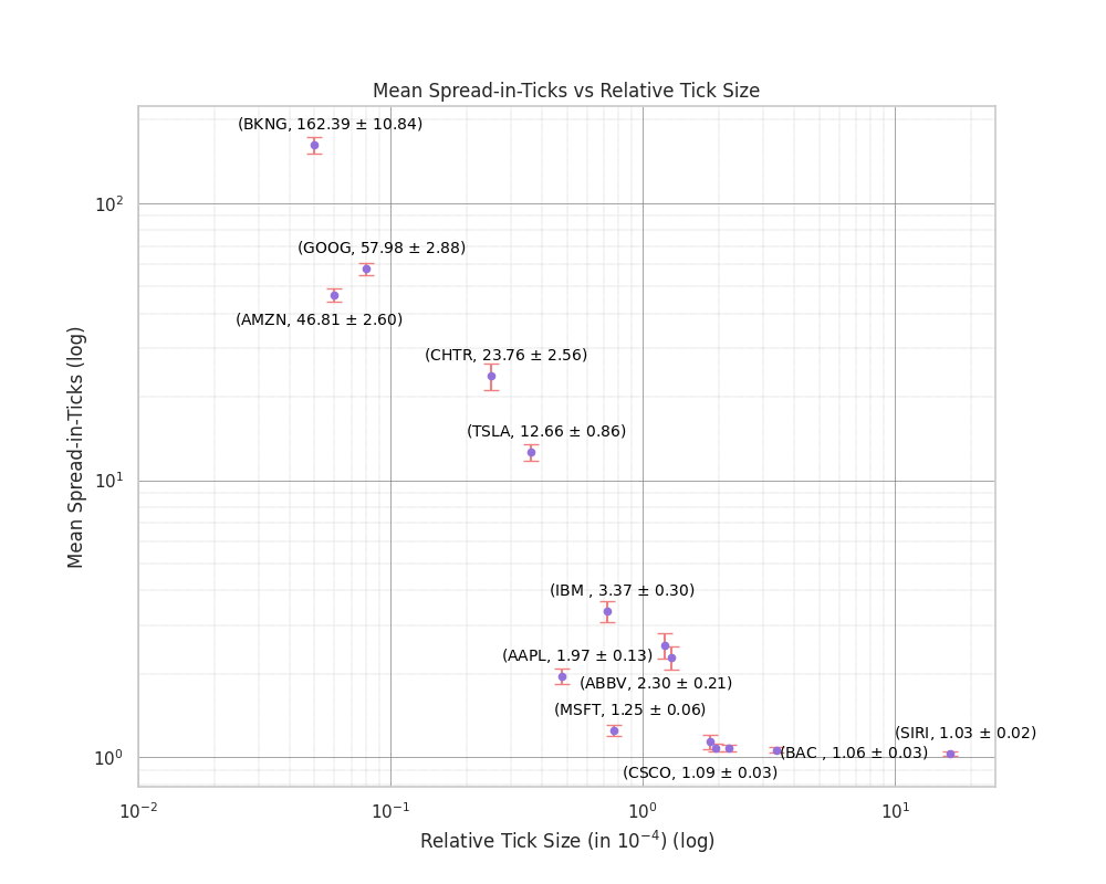
Figure 1: Mean Spread(in ticks) vs Relative Tick Size(in bps) : Annotations depict the stock’s mean and variance of the spread. Remarkably, the average spread seems to be highly correlated with the relative tick size, or, as noted by [5], by price. There are clearly two regimes here - since the spread can never be less than one tick, there is a flattening of this relation for large tick stocks, followed by a steady but noisy change to an almost linear (in log-log scale) relationship between the two for small and medium tick stocks.

As noted in [17], building a realistic and general Limit Order Book (LOB) model requires careful replication of the empirical density of spreads, both around the median and at the tails, as well as capturing the time-of-day dependence of spreads. This applies across stocks with varying relative tick sizes. Additionally, the price of a security plays a significant role in determining its mean spread, with some non-linearity observed in large-tick stocks due to the constraint that the spread cannot fall below one tick, as seen in [5] and in Figure 1.

Let the bid-ask spread $s(t)$ be the difference between the best ask price $p_{\text{ask}}(t)$ and the best bid price $p_{\text{bid}}(t)$ at time $t$ . Mathematically:

$$s(t)=p_{\text{ask}}(t)-p_{\text{bid}}(t)$$

We plot the average spread against the average price on a log-log scale to explore the relationship between price and spread.

We observe a gradual increase in the mean bid-ask spread as the relative tick size decreases across stocks in the dataset. For instance, the mean spread for INTC, a large-tick stock, is $1.02$, whereas for AMZN, a small-tick stock, it reaches $47.18$. In the log scale, the tail of the spread distribution is more pronounced for AMZN, with significant values persisting over dozens of ticks, while for INTC, it decays to near zero after just two ticks (Figure 21). To measure the difference in shapes of the spread distributions, we make use of the Weibull distribution as our candidate distribution. This choice is motivated by the empirical fact that with decreasing relative tick size, one observes the mode shifting from 1 tick to multiple ticks however the tail of the distribution dies quicker as well. Considering this, the Weibull distribution is a prime candidate. We make use of the method of moments to calculate the Coefficient of Variation or CV (i.e. variance divided by mean squared) of the empirical observed spreads for one calendar year. CV is governed by the shape parameter of the Weibull distribution alone ([8]) and therefore is a good statistic to measure the differences in shape across stocks. We show the relation of CV to the relative tick size in Figure 2 and we fit a linear regression line on this scatter plot (shown in red). One can clearly observe a definitive trend as we decrease the relative tick size, the slope of the red line is $-2.721$, and so we have the relation $CV\propto\text{(Rel. Tick-Size)}^{-2.7}$. Therefore we conclude that the shape of the spread distribution is directly related to the relative tick size of a stock.

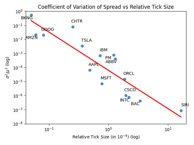
Figure 2: Spread Shape vs Rel. Tick Size: After using the Weibull distribution as a prior on the spread distribution, we plot here the variance divided by mean sqaured (also known as Coefficient of Variation (CV)). This parameter drives the shape of the Weibull distribution. As can be clearly seen here, the shape varies linearly (on a log-log scale) with relative tick size. As rel. tick size decreases, the shape of the spread distribution shifts from that similar to an exponential to one similar to log-normal.

In the time-of-day analysis, we observe tick-constrained dynamics in large-tick stocks like INTC, where the spread remains floored at one tick throughout the trading day, despite price discovery causing fluctuations in the spread. This behavior is markedly different in medium and small-tick stocks, where the spread exhibits more variation throughout the day.

3.2 Price Changes:

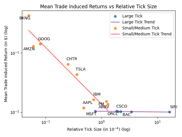
Figure 3: Mean of Trade induced Price Moves (in $): As we move from large tick stocks to medium and small tick, we exit the domain of half tick mid price moves to multiple ticks. This is an important observation since, for example, the volatility process (for absolute returns) is scaled by the mid-price changes’ scale which, as we show here, is determined by the rel. tick size. The slope of the small/medium tick fit is approximately $-1$. We therefore conclude that price moves are scaled by the current price which is a tenet in Geometric Brownian Motion models of the price process.

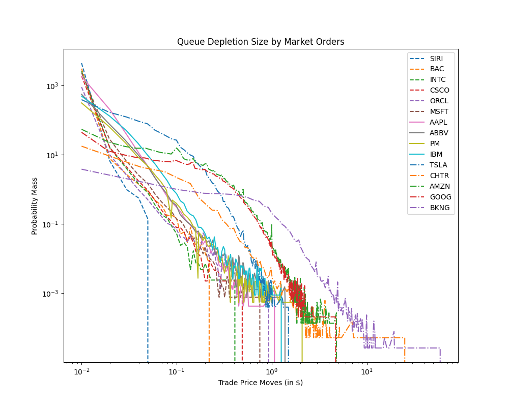
Figure 4: Histogram (log-log) of Trade induced Price Moves (in $): Notably the tail of all large (dashed lines) and medium (solid lines) tick stocks quickly dies quickly after half a tick however the distribution has a higher variance and a higher mode for small tick stocks (dash-dotted lines). This implies that it is not just the mean of the price changes that vary with rel. tick size but the shape of the distribution changes significantly as well.

Price changes are one of the most important events in an LOB since it either signifies a trade that has happened or a change in the best quotes. To measure the behavior of mid-price changes in the Limit Order Book (LOB), we analyze the impact of trades on the LOB. Specifically, if the size of a trade (i.e., a market order) exceeds the instantaneous volume at the top of the book on either the bid or ask side, it leads to a queue depletion event. The remainder of the market order’s volume will then be filled from deeper levels of the LOB. The ratio of the trade size to the instantaneous top-of-the-book volume reflects the liquidity available at the top of the book. We consider two key statistics: the distribution of this ratio and the average amount (in price levels) by which a market order depletes the LOB. These statistics serve as our stylized facts for mid-price changes in the LOB. We show the mean trade induced price moves against varying relative tick sizes in Figure 3. On a log-log scale, again, we see a clear linear relationship between the two for small and medium tick stocks. There is some non-linearity for large tick stocks since the absolute returns are floored at half a cent. We show this non-linearity by depicting two regressions - one for large tick stocks (purple line) and one for all other stocks (red line). The slope of the fit for small/medium tick stocks is $-0.95$. Since relative tick-size here is proportional to the price of the security, we therefore conclude that the mean trade induced price is almost linearly related to the current price of the security. This experiment verifies the utility of using geometric scaling for price process models (the most simple one being the Geometric Brownian Motion).

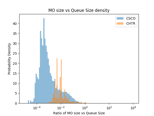
Figure 23: Market Order Size vs Instantaneous Volume at Best

Figure 23 demonstrates that as the relative tick size decreases, market orders deplete a larger proportion of the top quote size. This observation indicates that the top of the book in small-tick stocks is much more volatile compared to large-tick stocks. In Figure 4, we overlay the density of price moves resulting from a market order in the LOB. For large-tick stocks like SIRI, the probability of a price move exceeding one tick (e.g., one cent on the x-axis) is almost nonexistent. Conversely, for small-tick stocks, price moves of hundreds of ticks (e.g., one dollar) are relatively common. This discrepancy arises because the market order size relative to the top-of-the-book quotes is higher in small-tick stocks, combined with the fact that small-tick stocks typically have a sparser LOB. Sparse LOBs can lead to larger price moves due to queue depletion events.

Trade-induced mid-price moves are crucial for the price discovery process. The significant differences observed among various stocks in this stylized fact underscore the importance of accounting for such dynamics when choosing an LOB model. Additionally, it is important to note that the volatility process is scaled by the average magnitude of price changes. Models that do not account for multiple-tick price moves may underestimate the observed volatility.

3.3 Shape of the LOB:

In order to measure the distribution of available liquidity at various price points in a LOB, we count the total size of outstanding limit orders with respect to distance from the mid-price. This quantity, as a function of distance from mid-price, is what we define as the shape of the LOB. The shape of the Limit Order Book (LOB) plays a crucial role in understanding liquidity distribution. However, modeling deeper levels of the LOB increases both the dimensionality and complexity of the model, especially for small-tick stocks. In a generalized LOB model, it is essential to account for the vast variability in liquidity distribution across different relative tick sizes.

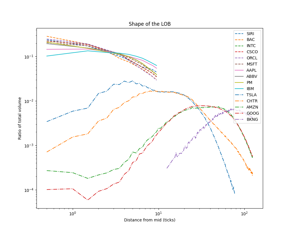
Figure 5: Shape of the LOB - empirical density (log-log): The tails of large (dashed) and medium (solid) tick stocks is insignificant beyond 10 ticks. This is due to the fact that our dataset contains only top 10 levels of the book and since the book is almost always dense in these stocks, there is virtually no probability mass for $>10$ ticks depth in our dataset. For small tick stocks (dash-dotted), we can clearly see a shift of the maxima to deeper levels as well as consistent shapes of the LOB.

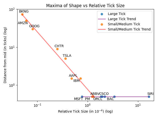
Figure 6: Depth with Maximum Liquidity of the LOB (log-log): Again we observe two regimes - the large tick names have the maximum liquidity at the top of the book however for small tick stocks, the maximum liquidity is correlated with the current rel. tick size as can be seen above. This correlation is power law with an exponent over rel. tick size of approximately $-1.5$.

Stock	25th Perc.	50th Perc.	75th Perc.
SIRI	1.1 $\pm$ 0.54	2.7 $\pm$ 0.88	5.2 $\pm$ 1.10
BAC	0.7 $\pm$ 0.42	2.2 $\pm$ 0.52	4.6 $\pm$ 0.62
INTC	1.3 $\pm$ 0.40	2.6 $\pm$ 0.35	5.1 $\pm$ 0.53
CSCO	1.3 $\pm$ 0.39	2.5 $\pm$ 0.29	5.0 $\pm$ 0.53
ORCL	1.1 $\pm$ 0.45	2.5 $\pm$ 0.33	4.6 $\pm$ 0.43
MSFT	1.5 $\pm$ 0.15	2.9 $\pm$ 0.43	5.5 $\pm$ 0.33
AAPL	1.8 $\pm$ 0.31	3.8 $\pm$ 0.43	6.5 $\pm$ 0.51
ABBV	1.6 $\pm$ 0.38	3.5 $\pm$ 0.55	6.1 $\pm$ 0.70
PM	1.6 $\pm$ 0.40	3.6 $\pm$ 0.61	6.4 $\pm$ 0.84
IBM	2.5 $\pm$ 0.66	4.9 $\pm$ 1.04	7.9 $\pm$ 1.36
TSLA	7.7 $\pm$ 2.63	15.0 $\pm$ 4.37	23.4 $\pm$ 5.80
CHTR	11.8 $\pm$ 2.51	20.4 $\pm$ 4.44	33.6 $\pm$ 9.27
AMZN	32.1 $\pm$ 6.32	49.2 $\pm$ 8.52	67.0 $\pm$ 10.45
GOOG	31.2 $\pm$ 6.20	47.6 $\pm$ 8.41	66.9 $\pm$ 10.23
BKNG	59.3 $\pm$ 8.01	78.6 $\pm$ 7.52	98.8 $\pm$ 5.95

Table 2: Shape Percentiles (in ticks)

Let the volume resting at a price level $p$ at time $t$ be denoted as $Q(p,t)$, which refers to the outstanding quotes at that price. The mid-price at time $t$ is denoted as $p_{\text{mid}}(t)$. We define the shape of the book as the time-weighted distribution of the volume $Q(p,t)$ as a function of the distance of the price level $p$ from the mid-price $p_{\text{mid}}(t)$. The shape of the book is calculated by first computing the volume at different price levels, weighted by the duration for which a particular shape persists. If a shape remains for 1 second, it is weighted 10 times more than one that persists for 0.1 seconds. The final distribution of volume for each day is referred to as the shape of the book for that day. Averaging over one calendar year gives the average shape of the book.

The shape of the book decays from its maximum at half a tick from the mid-price for large and medium-tick stocks, as illustrated in Figures 25(a) and 25(b). Notably, the shape profile decays more rapidly for large-tick stocks compared to medium-tick ones. For stocks like IBM, which are close to the boundary between medium and small-tick stocks, the maximum liquidity shifts deeper into the book. On the other hand, for small-tick stocks such as the one shown in Figure 25(c), the liquidity distribution is wider, with the maximum liquidity lying several ticks below the mid-price. Figure 5 further shows that within small-tick stocks, the shape becomes flatter as the relative tick size decreases.

Next, we calculate the maximum of the average shape of the book profile and show the results in Figure 6. As we can see, there are two regimes - large tick stocks have the maxima of the shape uniformly at half a tick away from the mid-price (fit shown in purple line). However we see an almost linear trend wherein the maximum liquidity shifts deeper in the book as we decrease the relative tick size (fit shown in red line). The slope of the red line is $-1.513$, therefore the relation is approximately power law with an exponent of $-1.5$ over the relative tick-size.

We also plot the empirical density of the instantaneous maxima to analyze the depth at which maximum liquidity lies in the LOB. The variability in the location of this maximum provides insights into how deep the liquidity is distributed in the book. The empirical density of the maxima of the liquidity as a function of distance from the mid-price, shown in Figure 26, indicates that the variance in the location of maximum liquidity increases as the relative tick size decreases. Even in small-tick stocks, there are significant instances where the maximum liquidity lies just half a tick from the mid-price. However, as depicted in Figure 21, the time-weighted likelihood of a one-tick wide spread is quite low.

In Table 2, we display the various percentiles of the shape of the book for the 15 stocks tested. This statistical summary provides further insights into the variability of the liquidity distribution across different stocks and relative tick sizes.

In summary, the shape of the LOB is a stylized fact that must be carefully modeled, particularly in the context of small-tick stocks, where the liquidity distribution exhibits significant variability and complexity.

3.4 Sparsity of the LOB:

A notable feature in small-tick stocks’ LOB is that not every price level in the LOB will have liquidity. We instead observe a number of empty price levels in the LOB (Figure 10) between two successive quotes. This implies that market participants are comfortable with placing their orders deeper in the LOB to post a more passive price. In large-tick assets, the probability of execution (also known as fill probability in literature) drastically decreases if one places an order deeper in the book. Small-tick assets clearly do not follow this trend. We therefore measure the sparseness of the LOB’s quoted prices in the following.

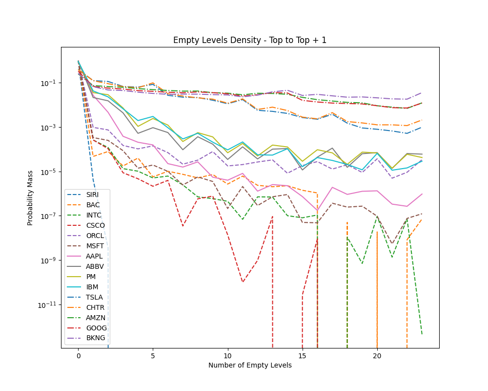
(a) Empty Levels between Top and Top + 1 (log density)

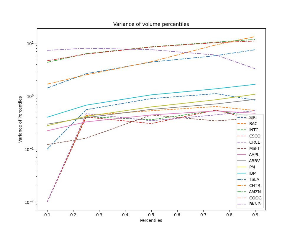
(b) Variance of Volume Percentiles (log)

Figure 7: Sparsity in the LOB: (a) depicts that the distribution of the number of empty levels becomes flatter as we decrease the rel. tick size. Indeed we can clearly observe that for large tick stocks (dashed lines), the distribution is very narrow and most of the mass is at 0. However for small tick (dash-dotted lines), there is a significant probability of more than 10 empty levels in the LOB. In (b) we show the variability in the instantaneous shape of the LOB by calculating the variance of the percentiles of the shape of the LOB. This measure informs us about the variation of liquidity in the book and therefore is a proxy measure for sparsity. As we can see in this figure, there is continous trend of increasing variance as we decrease the rel. tick size for all percentiles of the shape of the LOB.

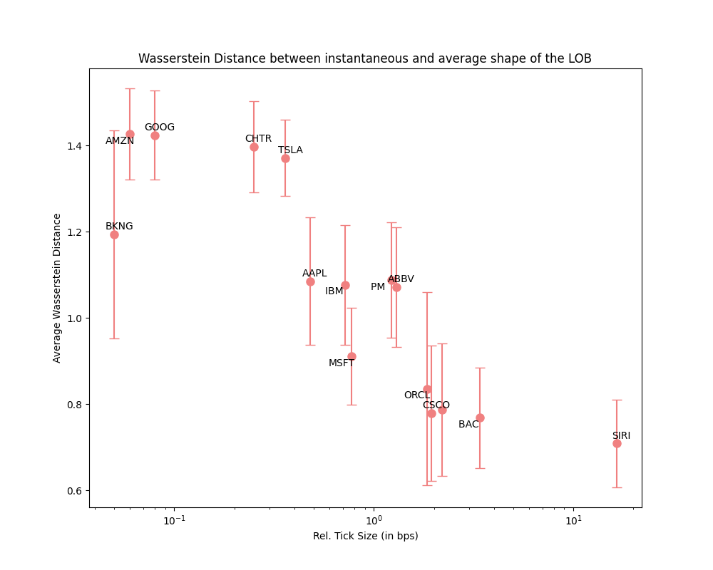
Figure 8: Instantaneous vs Average Shape of the LOB: This measure indicates how different, on a time-weighted average scale, is the instantaneous shape of the LOB from the average shape. This difference indicates whether the shape of the book remains persistent in the LOB or does the LOB’s liquidity vary a lot owing to the sparse levels in the LOB. As we can see clearly here, there is an increasing trend as we decrease the relative tick size however this relation seems to be non-linear.

We are interested in the number of empty levels between two quotes on either the ask or bid side of the book. Mathematically, let $n_{e}(p,t)$ denote the number of empty levels between two quotes at price level $p$ at time $t$. We calculate $n_{e}$ for the top ten quotes in the LOB on both a time-weighted daily average basis and an instantaneous basis. The time-series of the time-weighted daily mean, along with the empirical distribution (log-scaled) of the instantaneous number of empty levels, reveals a trend: as the relative tick size decreases, the distribution becomes flatter and heavier-tailed. This trend is evident in Figure 7(a), where the number of empty levels between the best and second-best quotes increases with decreasing relative tick size. Figure 22 further confirms that this pattern persists for deeper levels in the book.

Next, we calculate the percentiles of the shape of the book at the 10th, 25th, 75th, and 90th percentiles. The conjecture is that these percentiles will remain relatively invariant if the book is dense, meaning there are close to zero empty levels in the LOB. Thus, the variance of these percentile levels serves as a proxy measurement of the LOB’s sparsity. As shown in Figure 7(b), there is a steady relationship between the variance of the levels where certain percentages of total liquidity can be found and the relative tick size. This variance increases with decreasing tick size, indicating greater sparsity.

Finally, to measure sparsity robustly, especially against small orders lying between two price levels with significant quote sizes, we compute the Wasserstein Distance (or Earth-Mover’s Distance) between the average shape of the book and the instantaneous shape of the book. This metric helps differentiate between stocks where the average shape consists of sparse Dirac probability masses and those where both the average and instantaneous shapes are dense. Figure 8 illustrates a continuous increase in the Earth-Mover’s Distance with decreasing relative tick size, suggesting that the dissimilarity between average and instantaneous shapes increases as tick size decreases.

In summary, Figures 7(a) and 22, along with the calculations of percentiles and Wasserstein Distance, collectively indicate that the sparsity of the LOB increases as the relative tick size decreases. This finding underscores the challenge of accounting for sparsity in LOB models, as modeling order arrivals across numerous price levels, with potential correlations among them, presents a high-dimensional problem further complicated by lower signal-to-noise ratios at deeper levels in the book.

3.5 LOB Events and their Endogenous Excitation:

As previously discussed, a Limit Order Book can be modeled as a queuing system, where various types of events contribute to the formation and evolution of these queues. Empirical observations suggest that the realizations of these events exhibit both cross-correlation with other events and autocorrelation with themselves. This phenomenon is commonly referred to as market endogeneity ([5]), reflecting the idea that market activity is influenced by its own past behavior. Our focus lies in analyzing the conditional probability distribution of these events, given the history of prior events, in order to capture the feedback mechanisms inherent in the LOB dynamics.

We study how the occurrence of certain events in the Limit Order Book (LOB) affects the likelihood of other events happening shortly afterward. Specifically, we look at the probability of an event of type $e^{(1)}$ occurring within the next second after an event $e^{(2)}$ has just happened. This helps us understand how one type of event can ”trigger” or increase the chances of another type of event. We express this by calculating the ratio of this conditional probability (i.e., the chance of $e^{(1)}$ given $e^{(2)}$) to the overall probability of $e^{(1)}$ occurring in one second. This ratio is known as Conditional Probability Leverage. We perform this analysis for three types events : Limit Orders (LO), Cancel Orders (CO), and Market Orders (MO), and extend it to all events affecting the top 10 levels of the book.

Additionally, inspired by [21], we calculate the unconditional probability of various events (like Limit Orders, Immediate or Cancel Orders, etc.) happening at different distances from the mid-price. We denote these events by $e_{x}$, where $x$ is positive for events on the ask side and negative for events on the bid side. We then determine how likely it is for an event $e^{(1)}_{x}$ to occur given that a different event $e^{(2)}_{y}$ happened just before. We use this information to compute a measure called Leverage, which is the ratio of the conditional probability of $e^{(1)}_{x}$ following $e^{(2)}_{y}$ to the unconditional probability of $e^{(1)}_{x}$ i.e. $\frac{P(e^{(1)}_{x}|e^{(2)}_{y})}{P(e^{(1)}_{x})}$. We plot these results on a log scale for better clarity.

Figure 9 (and further Figure 24) show that the patterns in these leverage plots are similar across different tick sizes. This means that the way events influence each other is consistent, regardless of how large or small the tick size is. These findings provide insights into how the structure of the order book behaves and helps us understand the dynamics of event interactions within the LOB. Here we enlist some more observations from these plots:

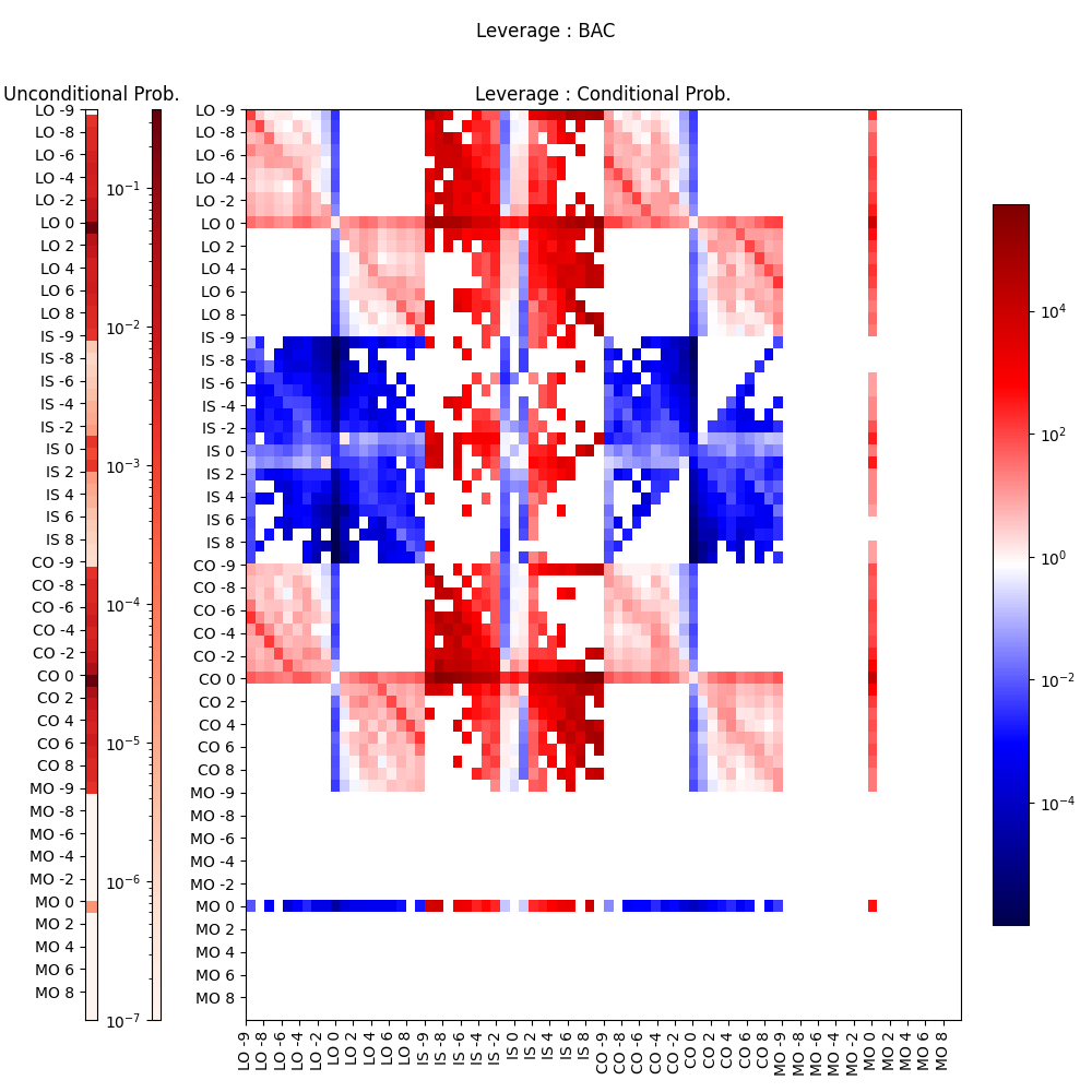
(a) BAC (Large tick)

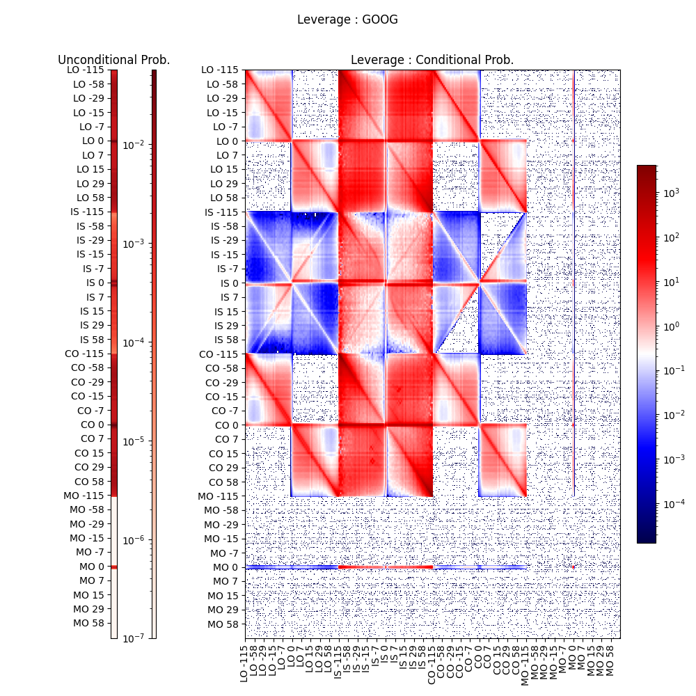
(b) GOOG (Small tick)

Figure 9: Leverage (from top): Darker the hue, more the leverage - The left hand side subplot shows the unconditional probability of the events while the leverage plot shows the conditional probability ratio. Note the similarities between the two figures (and further in Figure 24). This stylized fact motivates building a generalized self and cross excitory model for the 4 types of events shown here across all types of stocks, albeit with different scaling.

1. Limit Orders at the top of the book behave remarkably different to the deeper levels.

2. Cancels and Limit Orders behave very similar to each other.

3. Unsurprisingly, the unconditional probability of In-Spread Limit Orders (above 1 tick distance from the top) is very small for large and medium tick stocks.

4. In-Spread Limit Orders are both self excited and cross excited by opposite end LOs and COs.

5. In-Spread Limit Orders excite other events very differently between small and large tick stocks.

6. Market Orders only occur at the top of the book, however we can see very similar patterns across all types of stocks for Market Orders.

We therefore conclude that in-spread orders should be modelled differently for different types of stocks however there is uniformity in other order types’ behaviour. We observe that our choice of modelling the top of the book as a separate entity to the deeper part of the book has some support.

4 A Simple Model

Clearly in Section 3.5 we see that the events are endogenously excited by themselves. This stylized fact, along with the general applicability and versatility of the Hawkes Process as discussed in Section 2.3, is the main motivation of using a self exciting point process as our LOB model. We propose a model of the LOB dynamics where the events are driven through a multidimensional Hawkes Process and there exist some state variables (such as the top of the book volume at Ask) of the LOB which evolve along with the point process. As discussed in [16], a Hawkes model alone is unable to capture dynamics of a small tick order book. The assumptions of the model are as follows.

• Firstly, the LOB is dense (i.e. not sparse). There are no empty levels between the deep levels and the top level. This assumption clearly fails for small tick LOBs as we have shown in Section 3.4.

• Secondly, the price improvements, i.e. in-spread orders, happen uniformly at a 1 tick distance from the top of the book. This is clearly not the case in small tick stocks since price improvements happen in multiple ticks.

• Thirdly, the top of the book contains most of the liquidity of the LOB. As shown in Section 3.3, for small and some medium tick stocks, the maximum liquidity actually lies much deeper in the book.

• Finally, the assumption that events in the price levels other than the top two have no contribution to the LOB dynamics is too strong. Section 3.5 depicts the same.

Therefore in order to enhance this model and to relax these assumptions, we propose to create a model of the LOB which not only captures the top of the book dynamics but also is able to model the deeper price levels’ events. Simply increasing the dimensions of the Hawkes Process model to incorporate events in the deeper LOB, and to incorporate in-spread orders at all levels from top to the opposite side’s top, is infeasible. This is because the Hawkes Process calibration becomes exponentially harder as we increase the dimensions of the process. Even if we could calibrate the process, the question of model parsimony becomes important. Therefore we propose here to model events happening in a range of price levels as a single dimension in the Hawkes Process. The range of these ’fat queues’ is denoted by their ’width’. These widths are dynamic quantities which evolve with the events in the LOB. These width variables along with the queue sizes are what we call ’state variables’ of the LOB. We describe these state variables below and then propose a simple model where the parameters of the Hawkes Process and the LOB State Variables are independently calibrated.

4.1 Formulation:

From Section 3.5, it is clear that for all stocks, there needs to be a demarkation between the top of the book and the deeper levels, for both LOs and COs. This, along with LOs at the in-spread levels, and MOs, constitute all the dimensions of the book. The choice of how deep we would like to model the LOB is a pertinent question. As a heuristic, we choose the 50th percentile of the average shape of the LOB as our maximum depth that we would like to model. We define this quantity as $M_{0.5}$ which is a constant in time.

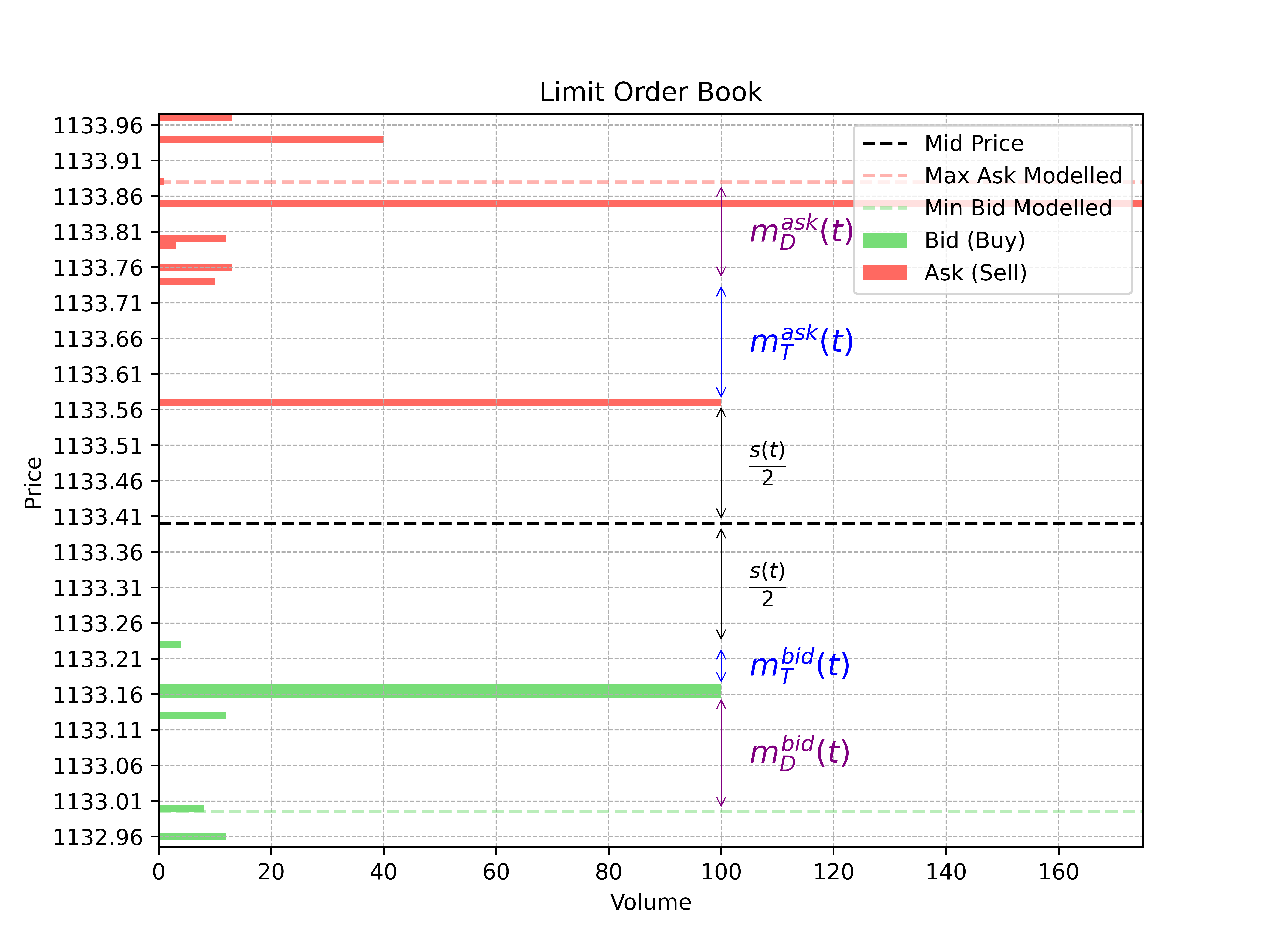
Figure 10: Example LOB State Variables: This is a random snapshot from GOOG’s LOB data. Notice the sparsity in the best quotes on both sides.

We define two width variables : $m^{(\zeta)}_{T}(t),m^{(\zeta)}_{D}(t)$ respectively denoting the width of the top price levels and the deeper price levels for $\zeta\in\{\text{bid, ask}\}$ being the side. The width is measured from the mid-price in ticks. $s(t)$ is defined as the instantaneous bid-ask spread-in-ticks. All five of these are random processes and their domain is $\frac{1}{2}\mathbb{N}$.

Definition 1.

$m^{(\zeta)}_{T}(t)$ is defined as the distance in-ticks between the top of the book at side $\zeta$ and the next best quote at the same side $\zeta$.

For example, in Figure 10, the the best ask quote is at 1133.57 $ and the second best quote is at 1133.74 $. Therefore $m^{(ask)}_{T}(t)=17$ ticks.

Definition 2.

$m^{(\zeta)}_{D}(t)$ is defined as the width of the deeper levels. This is a random process which evolves dynamically with the LOB events. We initiate this using $m^{(\zeta)}_{D}(0)=M_{0.5}-0.5s(0)-m^{(\zeta)}_{T}(0)$.

For example, in Figure 10, the second best ask quote is at 1133.74 $ and mid-price $+M_{0.5}$ is at 1133.88 $. Therefore $m^{(ask)}_{D}(t)=14$ ticks. This random process has a constraint that we can never have more than $M_{0.5}+1$ levels on each side of the book in the model. This choice is motivated by model parsimony as well as the hypothesis that any quotes deeper than $M_{0.5}$ ticks away from the mid-price have neglible contribution to the LOB’s top of the book dynamics. Mathematically, this constraint can be written as $M_{0.5}-0.5s(t)-m^{(\zeta)}_{T}(t)-m^{(\zeta)}_{D}(t)>=-1$ and $m^{(\zeta)}_{D}(t)>=1$. Therefore it is possible that while the LOB is evolving, the number of levels modelled (on each side) by these three fat-queues is much less than $M_{0.5}$. We discuss in the following how we maintain these constraints.

There are therefore three wide queues, at each side, we keep track of in this model - the in-spread queue (i.e. for Limit Orders arriving inside the spread), the top queue and the deeper queue. Each of these queues have a queue size which is the total order volume resting in the queue at that instant of time. Naturally, the queue size for in-spread queues is always zero. We denote the queue size at the top queue and the deeper queue by $Q^{(\zeta)}_{T}(t),Q^{(\zeta)}_{D}(t)$ respectively. These are again random processes with domain $\mathbb{N}$. There are total 12 events that can happen in these queues which are, on each side of the book, LOs in the three wide queues, COs in the two queues with non-zero queue size, and MOs at the top of the book. The set of events is:

$$\mathcal{E}:=\{LO_{\text{ask}_{D}},CO_{\text{ask}_{D}},LO_{\text{ask}_{T}},CO_{\text{ask}_{T}},MO_{\text{ask}_{T}},LO_{\text{ask}_{IS}},LO_{\text{bid}_{IS}},LO_{\text{bid}_{T}},CO_{\text{bid}_{T}},MO_{\text{bid}_{T}},LO_{\text{bid}_{D}},CO_{\text{bid}_{D}}\}$$

4.2 Methodology

Since the order book queues are not restricted to a single tick width, determining the precise price level at which a simulated order is placed at becomes a critical consideration. The Hawkes process model, incorporating the 12 aforementioned event types, provides the event time and type upon simulation, but does not specify the exact price associated with an order—particularly for LOS and COs. To address this, we derive difference equations for the LOB state variables corresponding to each event type. The subsequent section details the event types and their impact on this coarse-grained LOB representation.

1. $LO_{\zeta_{IS}}$:
   Since IS orders can arrive at any price point between the top of the book and the top of the opposing side, it is necessary to establish a methodology for determining the precise price point at which such an order will arrive. Let $\eta_{IS}\in\mathbb{N}$ be defined as the number of ticks from the top at side $\zeta$ where this new in-spread order arrives at. We sample this $\eta_{IS}$ from a calibrated stationary distribution $\Pi(\hat{\eta}_{IS})$ where $\hat{\eta}_{IS}$ is a calibrated parameter. We denote this relation as $\eta_{IS}(\in\mathbb{N})\sim\Pi(\hat{\eta}_{IS})$ from here onwards. $\eta_{IS}$ is capped at the current spread in ticks and floored by one tick. The choice of distribution shape and the calibration of the parameter $\hat{\eta}_{IS}$ is directly related to the stylized fact of sparsity showcased in section 3.4.

   Also, the order size of this new order $\kappa_{IS}\in\mathbb{N}$ is sampled from a calibrated stationary distribution $\Pi(\hat{\kappa}_{IS})$. This distribution of the order size can contain spikes at round numbers similar to the empirical observations found by [16].

   The following changes happen to the five random processes mentioned above:

   $$\eta_{IS} \sim\Pi(\hat{\eta}_{IS})$$ (1)

   $$m^{(\zeta)}_{T}(t^{+}) =\eta_{IS}$$ (2)

   $$m^{(\zeta)}_{D}(t^{+}) =m^{(\zeta)}_{D}(t)+m^{(\zeta)}_{T}(t)$$ (3)

   $$Q^{(\zeta)}_{T}(t^{+}) =\kappa_{IS}$$ (4)

   $$Q^{(\zeta)}_{D}(t^{+}) =Q^{(\zeta)}_{T}(t)+Q^{(\zeta)}_{D}(t)$$ (5)

   $$s(t^{+}) =s(t)-\eta_{IS}$$ (6)

   

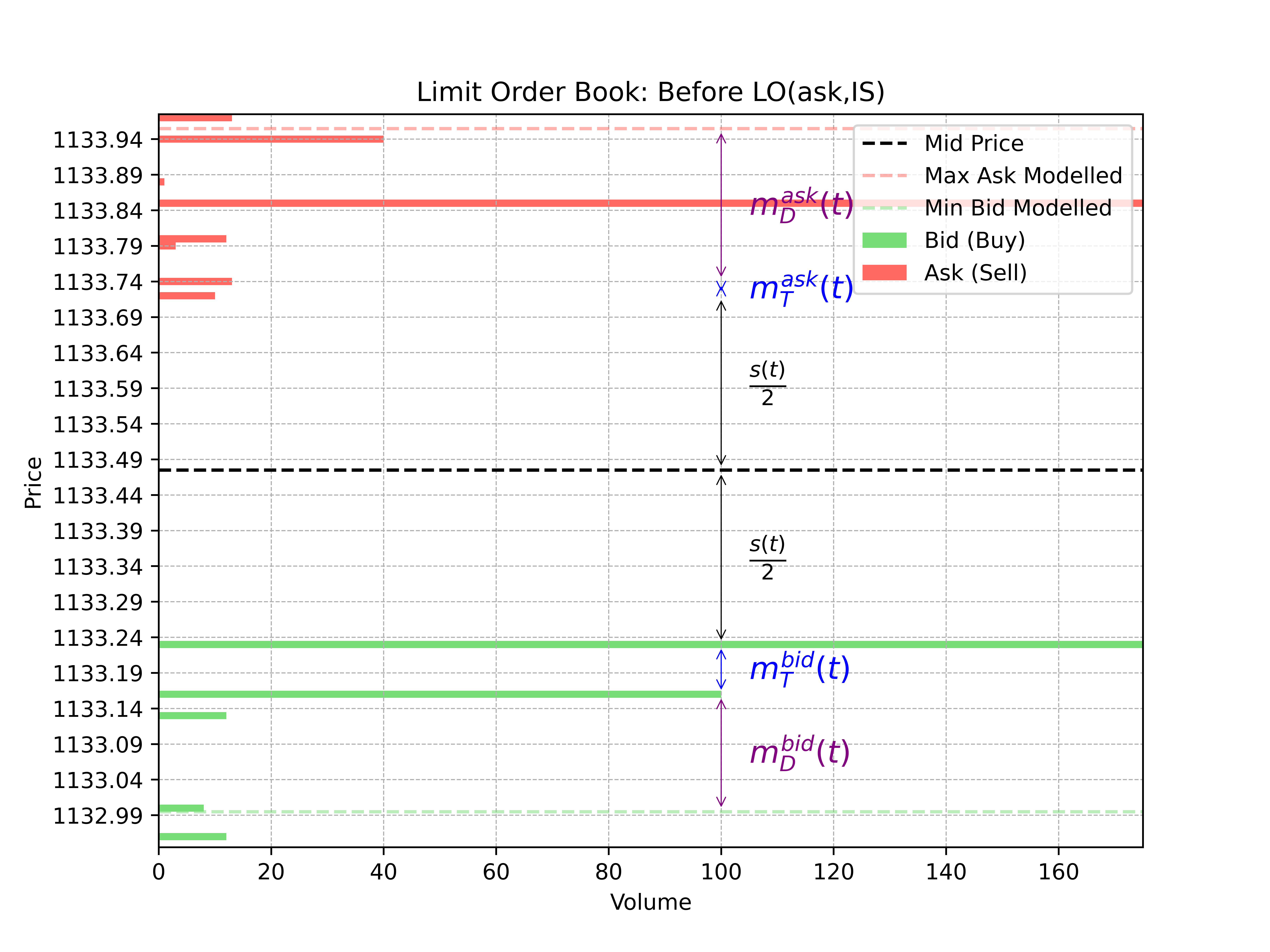
   (a) Pre-event

   

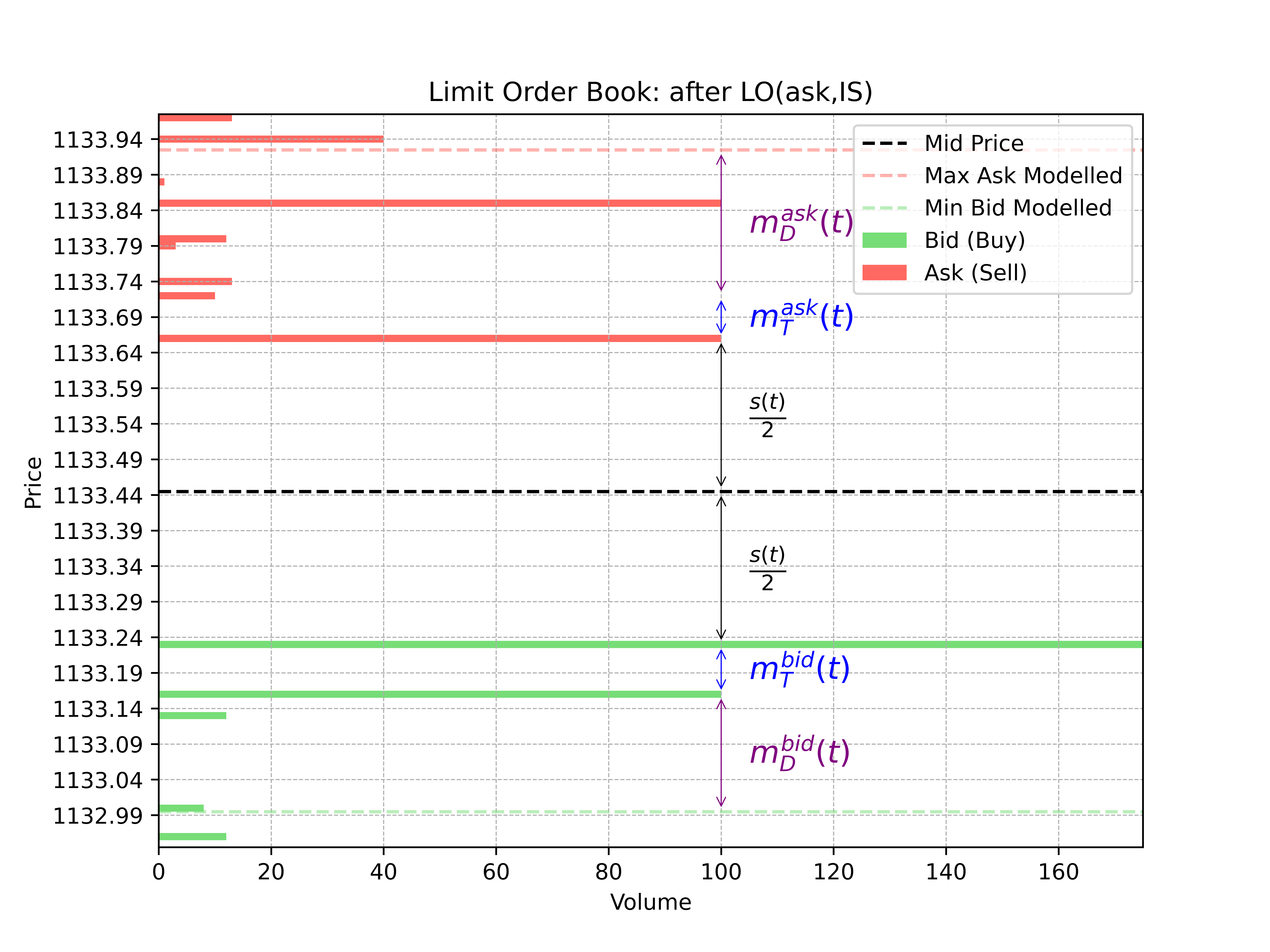
   (b) Post-event

   Figure 11: $LO_{\zeta_{IS}}$: Ask side In-Spread LO occurs at 1133.66 $

   Since this event is an event which increases $m^{(\zeta)}_{D}(t)$, we need to check the constraint mentioned in Definition 3. If the constraint is violated, we do the following purging of the width of the deeper levels to maintain the constraint of modelling at most the top $M_{0.5}$ levels in the LOB.

   $$m^{(\zeta)}_{D}(t^{+}) =M_{0.5}-0.5s(t^{+})-m^{(\zeta)}_{T}(t^{+})$$ (8)

   $$Q^{(\zeta)}_{D}(t^{+}) =Q^{(\zeta)}_{D}(t^{+})-\Delta Q^{(\zeta)}_{D}(t)$$ (9)

   $$\Delta Q^{(\zeta)}_{D}(t) =\text{Partition}(Q^{(\zeta)}_{D}(t),m^{(\zeta)}_{D}(t^{+})-m^{(\zeta)}_{T}(t),m^{(\zeta)}_{D}(t))$$ (10)

   Here $\Delta Q^{(\zeta)}_{D}(t)$ is defined as a partition of the existing $Q^{(\zeta)}_{D}(t)$. This partition directly depends on the number of levels in the partition ($m^{(\zeta)}_{D}(t^{+})-m^{(\zeta)}_{T}(t)$) and the number of levels in the parent ($m^{(\zeta)}_{D}(t)$). Figure 11 shows the same logic pictorially. In this instance, a new in-spread order arrives at the price point of 1133.66 $, corresponding to $\eta_{IS}=6$ ticks. According to equation (2), the mid-price jump $m^{(\zeta)}_{T}(t^{+})$ increases to 6 ticks from the previous 2 ticks. However, the deep width variable $m^{(\zeta)}_{D}(t)$ cannot be further increased, as doing so would exceed the modeled levels limit (indicated by the dashed red line). Consequently, the orders at the price level of 1133.94 $ are purged, ensuring that $m^{(\zeta)}_{D}(t^{+})$ no longer violates this constraint. This example is derived from a real Limit Order Book (LOB) in our dataset. In the Hawkes process simulations, this level of fine-grained information in the deep dimension is unavailable. Therefore, it becomes necessary to purge using a partition function based on an assumed liquidity distribution at the deeper levels. This partition function can be calibrated according to the shape of the order book, as outlined in section 3.3.

2. $LO_{\zeta_{T}}$:
   Since the top of the book consists of multiple price levels, we need to follow the same strategy as above to define which price level the LO will arrive at. Let $\eta_{T}(\in\mathbb{N})\sim\Pi(\hat{\eta}_{T})$ be defined as the number of ticks from the top at side $\zeta$ where this new order arrives at. $\eta_{T}$ is capped at $m^{(\zeta)}_{T}(t)$ and floored at zero. Again, the calibration of the distribution shape and the parameter can be informed using the sparsity stylized facts measured in section 3.4. Finally, $\kappa_{T}(\in\mathbb{N})\sim\Pi(\hat{\kappa}_{T})$ is the order size of this LO. If $\eta_{T}$ is 0, the LO is simply added to the existing queue at the top and no changes occur in the 5 processes except $Q^{(\zeta)}_{T}(t^{+})=Q^{(\zeta)}_{T}(t)+\kappa_{T}$. Otherwise, the following changes happen to the random processes mentioned above:

   $$\eta_{T} \sim\Pi(\hat{\eta}_{T})$$ (11)

   $$\text{if }\eta_{T}\text{ is }0,\qquad$$

   $$Q^{(\zeta)}_{T}(t^{+}) =Q^{(\zeta)}_{T}(t)+\kappa_{T}$$ (12)

   else,

   $$m^{(\zeta)}_{T}(t^{+}) =\eta_{T}$$ (13)

   $$m^{(\zeta)}_{D}(t^{+}) =m^{(\zeta)}_{D}(t)+m^{(\zeta)}_{T}(t)-\eta_{T}$$ (14)

   $$Q^{(\zeta)}_{D}(t^{+}) =Q^{(\zeta)}_{D}(t)+\kappa_{T}$$ (15)

3. $CO_{\zeta_{T}}$:
   If the CO does not lead to a queue depletion, i.e. if the number of orders at the top is more than one, then we randomly select some quantity from the existing queue at the top and cancel that quantity. The top of the book queue size changes as follows $Q^{(\zeta)}_{T}(t^{+})=Q^{(\zeta)}_{T}(t)-\kappa_{CO}$ where $\kappa_{CO}$ is the randomly selected quantity. If the CO leads to a queue depletion (QD), we need to calculate the new top of the book width as well as deplete the deeper fat queue by this new top level’s total volume. Assuming a sparse structure within the deep fat queue (informed by section 3.4), we sample a random new top width denoted by $\eta_{T+1}$. To calculate the total volume at this new level, we make use of the partition function mentioned earlier to deplete the deep fat queue. Mathematically, we perform the following to redefine a new top of the book.

   $$m^{(\zeta)}_{T}(t^{+}) =\eta_{T+1}$$ (16)

   $$m^{(\zeta)}_{D}(t^{+}) =m^{(\zeta)}_{D}(t)-m^{(\zeta)}_{T}(t^{+})$$ (17)

   $$Q^{(\zeta)}_{T}(t^{+}) =\text{Partition}(Q^{(\zeta)}_{D}(t),m^{(\zeta)}_{T}(t^{+}),m^{(\zeta)}_{D}(t))$$ (18)

   $$Q^{(\zeta)}_{D}(t^{+}) =Q^{(\zeta)}_{D}(t)-Q^{(\zeta)}_{T}(t^{+})$$ (19)

   Here, $\eta_{T+1}(\in\mathbb{N})\sim\Pi(\hat{\eta}_{T+1})$ is defined as the number of levels the new top has after the queue depletion event.

4. $MO_{\zeta}$:
   Market Orders, mathematically, behave exactly the same as Cancel Orders. If the size of the market order $\kappa_{MO}(\in\mathbb{N})\sim\Pi(\hat{\kappa}_{MO})$ is less than the existing queue size, there is a simple reduction in volume at the top, according to time priority, and we report a trade. The top of the book queue size changes as follows $Q^{(\zeta)}_{T}(t^{+})=Q^{(\zeta)}_{T}(t)-\kappa_{MO}$. If the MO leads to a queue depletion, the same logical waterfall as the one above is followed. If a market order depletes more than one price level, we repeat the process until we completely execute the MO quantity. Thus a MO can deplete multiple price levels using this methodology. This clearly means that the stylized facts related to the price moves induced by trades 3.2 is modelled implicitly.

5. $LO_{\zeta_{D}}$:
   Since we do not keep track of the fine grained orders or price levels in the deeper dimension, we simply increment the total volume present there with this new LO size $\kappa_{D}(\in\mathbb{N})\sim\Pi(\hat{\kappa}_{D})$.

   $$Q^{(\zeta)}_{D}(t^{+}) =Q^{(\zeta)}_{D}(t)+\kappa_{D}$$ (20)

6. $CO_{\zeta_{D}}$:
   In case of a QD event, if $m^{(\zeta)}_{D}(t)+m^{(\zeta)}_{T}(t)+0.5s(t)\leq M_{0.5}$, i.e. the width of the deep fat queue is not violating the constraint in Defintion 3, we absorb the new empty levels in $m^{(\zeta)}_{T}(t)$ and create a new deep fat queue with the following width and volume:

   $$m^{(\zeta)}_{D}(t^{+}) =M_{0.5}-m^{(\zeta)}_{T}(t)-0.5s(t)$$ (21)

   $$Q^{(\zeta)}_{D}(t^{+}) \sim\Pi(\hat{Q}_{D},m^{(\zeta)}_{D}(t^{+}))$$ (22)

   $$m^{(\zeta)}_{T}(t^{+}) =m^{(\zeta)}_{T}(t)+m^{(\zeta)}_{D}(t)$$ (23)

   If the constraint is violated, we set $m^{(\zeta)}_{D}(t^{+})$ to 1, sample $Q^{(\zeta)}_{D}(t^{+})$ from $\Pi(\hat{Q}_{D},m^{(\zeta)}_{D}(t^{+}))$ and let the deeper queue have just one non empty level since we cannot go deeper than $M_{0.5}+1$ in total depth of the LOB.

The 12 events form a mutually exciting 12 dimensional Hawkes Process with their intensities as follows from [16]. For $i=1\ldots 12,d=12$, let a $d$-dimensional Hawkes process have as the intensity of the process $\lambda^{(i)}(t)$ and the associated counting process $N^{(i)}(t)$ for $i=1,\ldots,d$. Here, $\mu^{(i)}$ is the exogenous intensity of the $i$-th dimension and $\phi^{(j\rightarrow i)}(t)$ is the excitation term from $j$-th dimension to $i$-th dimension. $\alpha$ is defined as the scale parameter for the in-spread intensity and $\beta$ is defined as the shape parameter.

For In-Spread events:

$$\lambda^{(i)}(t)= max\bigg{(}0,\bigg{(}\frac{s(t)-1}{\alpha}\bigg{)}^{\beta}\times\bigg{(}\mu^{(i)}+\sum^{d}_{j=1}\int^{t}_{0}\phi^{(j\rightarrow i)}(t-u)dN^{(j)}(u)\bigg{)}\bigg{)}$$ (24)

For other events:

$$\lambda^{(i)}(t)= max\bigg{(}0,\bigg{(}\mu^{(i)}+\sum^{d}_{j=1}\int^{t}_{0}\phi^{(j\rightarrow i)}(t-u)dN^{(j)}(u)\bigg{)}\bigg{)}$$ (25)

4.3 Calibration:

Since the Hawkes Dynamics is assumed to be independent of the LOB state variables, and since the distributions of the order sizes, order distances from top and queue sizes are unconditional on any state variable and stationary, we can decouple the calibration to a parametric estimation of the distributions and a non-parametric estimation of the Hawkes kernels. We suggest the methodology described in [16], combining [18] and [3], for the latter. The authors also provide visualization of the estimated kernel norms for INTC (Large Tick), AAPL (Medium Tick), TSLA and AMZN (Small Tick). For the former, we suggest making use of the Maximum Likelihood method with a prior that all these distributions are Geometric distributions. In Figure 12, we showcase the three $\eta$s distributions (note the shape looks exactly like the Geometric distribution) and their calibrated parameter: $\hat{\eta}_{(.)}$ across three stocks: INTC (large tick), AAPL (medium tick) and GOOG (small tick). Optionally, following [16, 21], one can add spikes in the probability distribution function to account for the traders’ preference of round numbers in the order sizes and queue sizes. For the partition functions, in the following section, we make use of a simple linear partition function - i.e. we assume that the shape of the book in the deeper LOB is flat. This is clearly a strong assumption (Section 3.2), and a better choice could be using the average shape of the book instead.

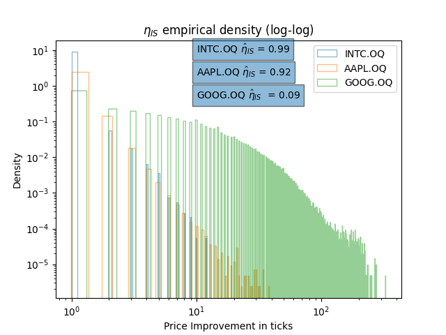
(a) $\hat{\eta}_{IS}$ Calibration

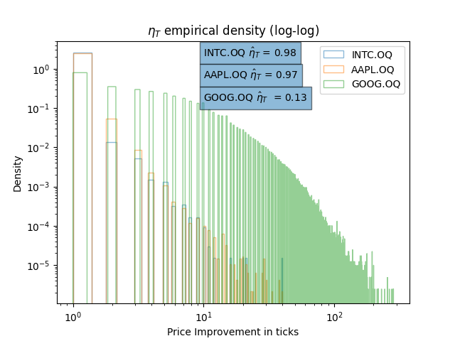
(b) $\hat{\eta}_{T}$ Calibration

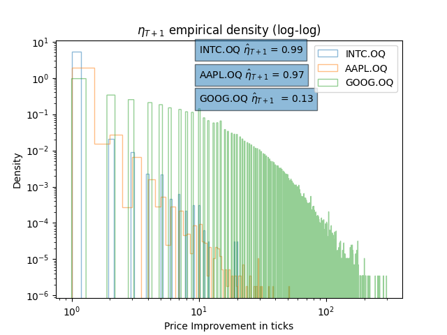
(c) $\hat{\eta}_{T+1}$ Calibration

Figure 12: $\hat{\eta}_{(.)}$ Calibration: $\hat{\eta}_{(.)}$ is the parameter which controls the sparsity of the LOB. Here we show three examples, one from each category of stocks, of empirical histograms of the sparsity levels. On a log-log scale it can be clearly seen that the distribution is similar to the geometric distribution. Inset we also show the calibrated parameters with this prior for all three stocks - we observe the calibrated parameters move from near one to near zero as we decrease the rel. tick size. This indicates an increase in sparsity with a decrease in rel. tick size.

5 Results

5.1 Stylized Facts:

In this section we describe the dynamics of the stylized facts defined above in Section 3 from the above model formulation.

5.1.1 Bid-Ask Spread and Price Moves:

It is easy to see that the spread process is decreased by $\eta_{IS}$ whenever an in-spread LO occurs and increased by $m^{(\zeta)}_{T}(t)$ whenever a queue depletion event (QD) occurs on side $\zeta$. Therefore we can write the differential equation of spread as:

$$ds(t) =\sum_{\zeta}\bigg{(}-\eta_{IS}dN_{LO_{\zeta_{IS}}}(t)+m^{(\zeta)}_{T}(t)\mathbbm{1}_{(QD^{(\zeta)})}(t)\big{(}dN_{CO_{\zeta_{T}}}(t)+dN_{MO_{\zeta}}(t)\big{)}\bigg{)}$$ (26)

Here $\mathbbm{1}_{(QD^{(\zeta)})}(t)$ is the indicator function for a QD event at side $\zeta$. As can be seen from the above, the spread process follows a jumpy point process methodology. Similarly the mid-price changes $dp(t)$ follow another jumpy point process. The only change is that while the spread is symmetrically changed by events in both the sides of the LOB, price changes happen anti-symmetrically. That is, an in-spread order at Ask side would decrease the mid-price but at the Bid side, it would increase the mid-price.

$$dp(t) =\sum_{\zeta}\frac{g(\zeta)}{2}\bigg{(}-\eta_{IS}dN_{LO_{\zeta_{IS}}}(t)+m^{(\zeta)}_{T}(t)\mathbbm{1}_{(QD^{(\zeta)})}(t)\big{(}dN_{CO_{\zeta_{T}}}(t)+dN_{MO_{\zeta}}(t)\big{)}\bigg{)}$$ (27)

Here we define $g:\{ask,bid\}\rightarrow\{1,-1\}$ as a signum function over the two sides with $g(ask)=1$ and $g(bid)=-1$. It is clear that for large and medium tick stocks where price improvements of IS orders happen uniformly at 1 tick and the width of the top is 1 tick as well, we can see that the bid ask spread will change by 1 tick at an event. For small tick stocks we can expect multiple tick moves in the spread process governed both by the distribution of $\eta_{IS}$ as well as $m^{(\zeta)}_{T}(t)$.

5.1.2 Shape and Sparsity of the LOB:

Let the volume available at a distance $x$ ticks away from the mid price be denoted by $q^{(\zeta)}(x,t)$ at an instant $t$.

$$q^{(\zeta)}(x,t) =Q^{(\zeta)}_{T}(t)\mathbbm{1}_{x=0.5s(t)}(t)+\frac{Q^{(\zeta)}_{D}(t)}{m^{(\zeta)}_{D}(t)}\mathbbm{1}_{x\geq 0.5s(t)+m^{(\zeta)}_{T}(t)}(t)$$ (28)

As can be seen from this, the shape of the book’s maxima will depend on the dynamics of $s(t)$ and $m^{(\zeta)}_{T}(t)$. Another noteworthy aspect from the above is that the instantaneous value of $q^{(\zeta)}(x,t)$ will be zero for $x\leq 0.5*s(t)$ which for small tick stocks means that the shape of the book will be increasing as we go deeper from the mid-price. In terms of sparsity, again the same fact that the book is empty from the mid-price to the top and again from the top of the book till the deeper level starts, sparsity should be replicated in the model as well.

5.2 Simulation Study:

Using the model specified above, we simulate an order book with random Hawkes and LOB Parameters. In Figure 13(a), we show a sample of the simulated order book for a small tick configuration of the parameters. We select the Hawkes Parameters by taking a power law kernel of the form $\phi^{(.)}(t)=a(1+ct)^{-b}$ with values for parameters $a,b,c$ for the kernels and the exogenous intensities chosen from the calibrated results on AMZN.OQ from [16]. The exact parameter specification is given in Appendix B. Note that this choice is purely driven by having a baseline LOB which makes logical sense (for eg, for a stable spread process, we require the rates of MOs and COs to approximately nullify the rates of LOs). We reflect the parameters of the Ask side to the Bid side to maintain model’s symmetry. For In-spread events, we choose $\alpha=95,\beta=0.6$ to be corresponding to a small-tick stock for this study. Following [16], we choose geometric distributions for order sizes $\kappa_{(.)}$ with spikes at round numbers like 1, 10, and 100. Similarly for unseen queue sizes, we use the geometric distribution with spikes at 1, 10, 100, 500 and 1000. Next, for $\eta_{(.)}$, we choose the geometric distribution again (with no spikes) since empirical observations (Figure 7(a)) show that the distance between top and top + 1 levels seem to follow an exponential distribution.

We vary each of the parameters on a range of values and showcase the fact that this model is general enough to be able to simulate characteristics of all kinds of stocks regardless of their relative tick size.

5.2.1 Ergodicity:

We vary the initialization of the LOB and check for stationarity in the evolution of the LOB dynamics. In Figure 13(b), we vary the initial spread for a small-tick parameter configuration and observe that the spread quickly converges to the mean spread of the LOB process. In Figure 13(c), we vary the initial sparsity of the LOB model by varying the parameter $M0:=(M0_{T},M0_{D})$. We initialise the LOB’s $m_{T}(0),m_{D}(0)$ using the exponential distribution with parameters $M0_{T},M0_{D}$ respectively. We plot the the distribution of $m_{D}(t)$ and see that the distribution remains invariant of the choice of $M0$. These two figures reinforce our claim that the process formed from the dynamics illustrated above is ergodic.

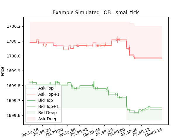
(a) Example LOB Simulations

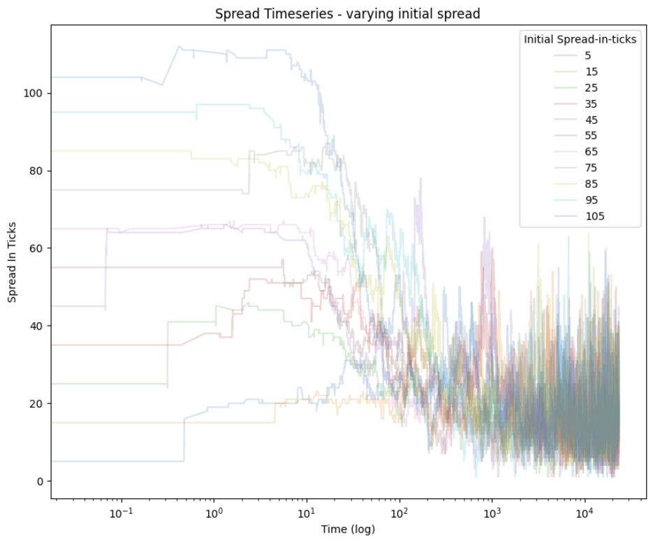
(b) Spread Timeseries: Varying $s(0)$ in the simulations

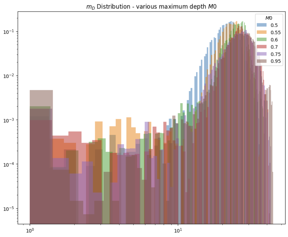
(c) Width of deep levels: Varying initial sparsity in the simulations

Figure 13: Simulation Study (Part 1): (a) showcases an example simulated coarse grained LOB - notice the spread is around 20-30 ticks and the top and top+1 levels have several empty levels as well. In (b) we do an ergodicity study for the spread time series by perturbing the initial spread of the simulation. Similarly in (c) we show the invariance of the distribution of $m_{D}(t)$ with various initial levels of sparsity.

5.2.2 Relative tick-size:

As can be seen in Equation 24, the in-spread events have two extra parameters $\alpha$ and $\beta$ which we respectively denote by AvgSpread and SpreadBeta. We postulate that controlling this parameter is vital for simulating LOBs of various relative tick sizes. In Figures 14(a) and 14(b), we can clearly see that varying this parameter gives us the characteristics of large, medium and small tick stocks respectively. However we note that absolute returns and sparsity is unchanged in these simulations (Figures 14(c) and 14(d)). To classify the simulations into small and large tick based on the spread distribution, we make use of the method of moments to calculate the shape parameter $k$ of the Weibull distribution. This is due to the fact that the Weibull distribution has a shape parameter $k$ which can control the distribution to look like an exponential distribution or like a log-normal. We plot the categories based on the classifier $k>1$ for small-tick assets and the rest for large-tick assets in Figure 15(a). We can clearly infer from the diagram that if we set $\beta$ to zero, i.e. make the in-spread orders’ intensity independent of the current spread, it is impossible to simulate a small tick order book. Finally we note that even though we see $k>1$ in all tests run with $\beta=0.9$, the mode of the spread observed in the simulations with $\alpha\leq 10$ ticks is still one-tick. This makes the simulated time series of spread very much alike to a large tick stock however the distribution of spread has a longer tail than the exponential distribution.

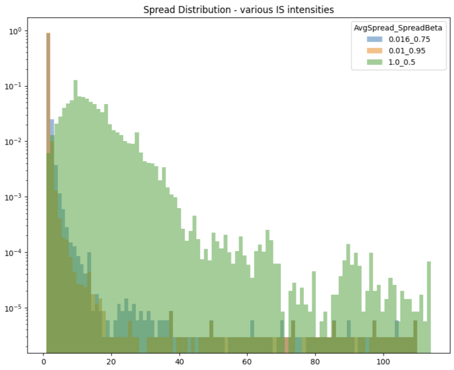
(a) Spread Distribution: Varying IS Hawkes parameters

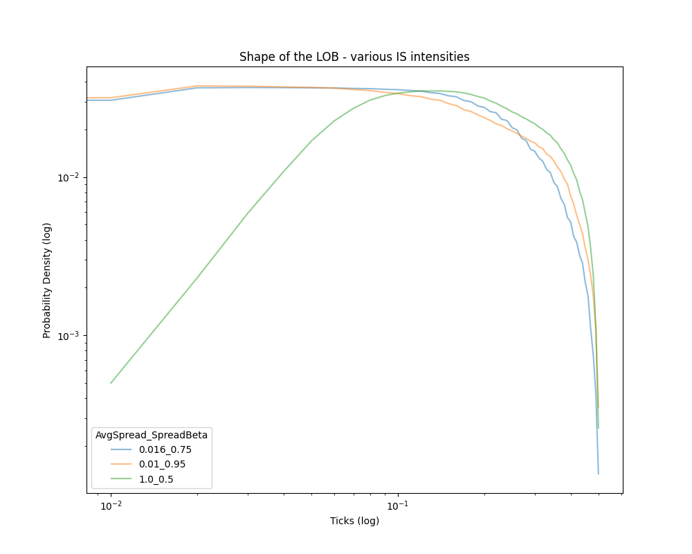
(b) Shape of LOB: Varying IS Hawkes parameters

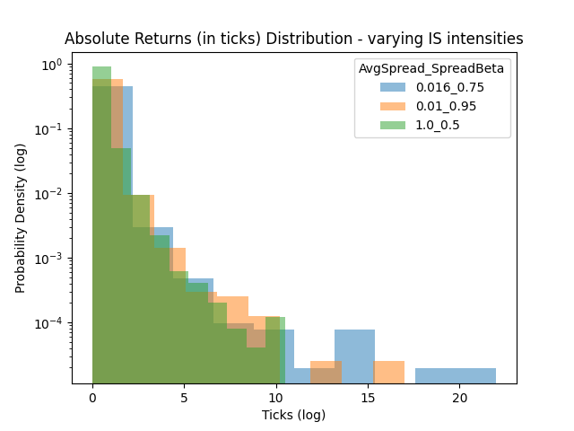
(c) Abs Returns Distribution: Varying IS Hawkes parameters

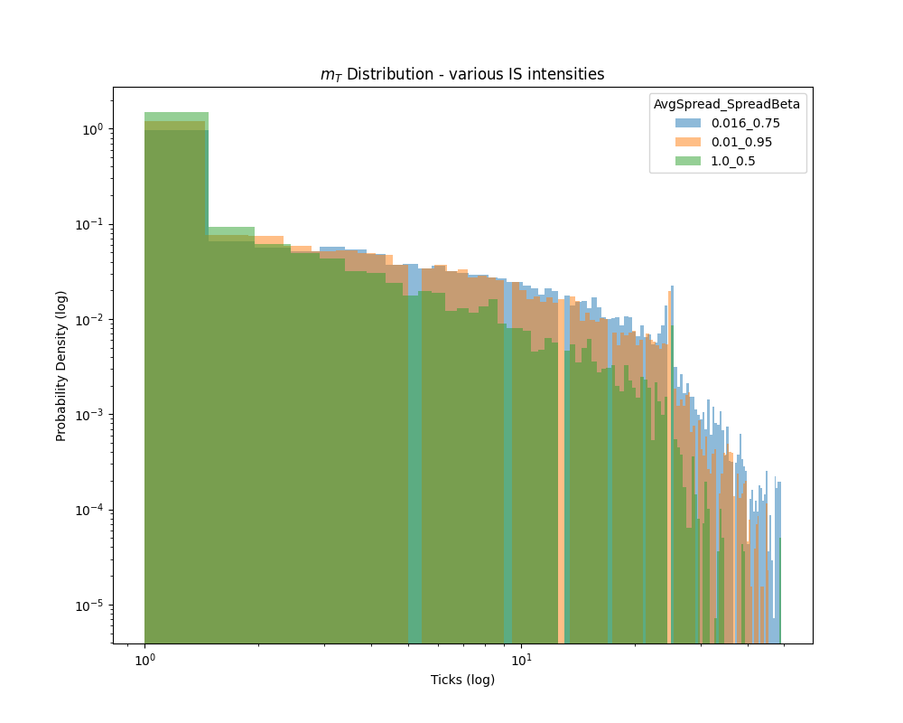
(d) Distance between top and top + 1: Varying IS Hawkes parameters

Figure 14: Simulation Study (Part 2): In (a) we vary the IS Hawkes Parameters $\alpha,\beta$ (also known as AvgSpread, SpreadBeta resp.) and we can see the distribution of spread changes from one that looks similar to the exponential distribution to one that looks more like a log-normal distribution. The average shape of the LOB (in a coarse grained sense) is plotted in (b) for varying AvgSpread and SpreadBeta. We can clearly see the shift of the maximum liquidity from the top of the book (i.e. half tick away from mid price) to much deeper in the book as we decrease SpreadBeta and increase AvgSpread. In (c) and (d) we show that controlling these two parameters alone does not account for the returns distribution’s shape as well as the distribution of the state variable $m_{T}(t)$ to a very good extent.

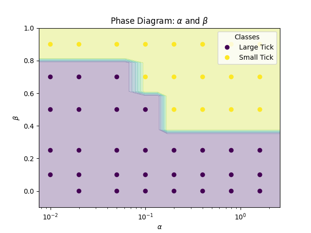
(a) Relative tick-size: Simulated

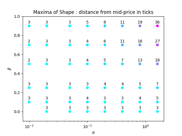
(b) Maxima of Shape: Simulated

Figure 15: Phase Diagrams of varying In-Spread Hawkes Parameters $\alpha,\beta$: Previously we noted that several stylized facts depend heavily on the parameter choice of $\alpha\&\beta$. In these charts we show a grid of varying $\alpha\&\beta$ with a classification between Large and Small tick characteristics in the simulated LOB based on the spread distribution’s shape as well as based on the depth of the maximum liquidity in the LOB. Clearly, both the parameters are crucial in defining the tick-ness of the stock.

This leads us to the next crucial parameter for changing the relative tick-size of the simulated LOB - $\hat{\eta}_{(.)}$. This parameter controls the number of empty levels between two queues in the LOB and therefore is directly related to sparsity. We vary it from 0 to 1 where near one $\hat{\eta}$ would mean that, for example, the price improvements due to in-spread limit orders is always 1 tick and near zero $\hat{\eta}$ would correspond to price improvements happening randomly from 1 tick to spread-in-ticks. In Figures 16(a), 16(c), 16(d) and 16(b), we can see that varying this parameter leads to varying relative tick-size of the simulated LOBs even though the in-spread order intensity parameters ($\alpha,\beta$) are corresponding to that of a small-tick stock. Therefore we conclude that it is critical to calibrate both the $\alpha,\beta$ and $\hat{\eta}_{(.)}$ accurately. In terms of modelling the deeper part of the LOB, we show in Figures 16(e) and 16(f), that varying the sparsity levels can vary the variance of $m_{D}$ and the shape quite closely resembles that of the empirical data.

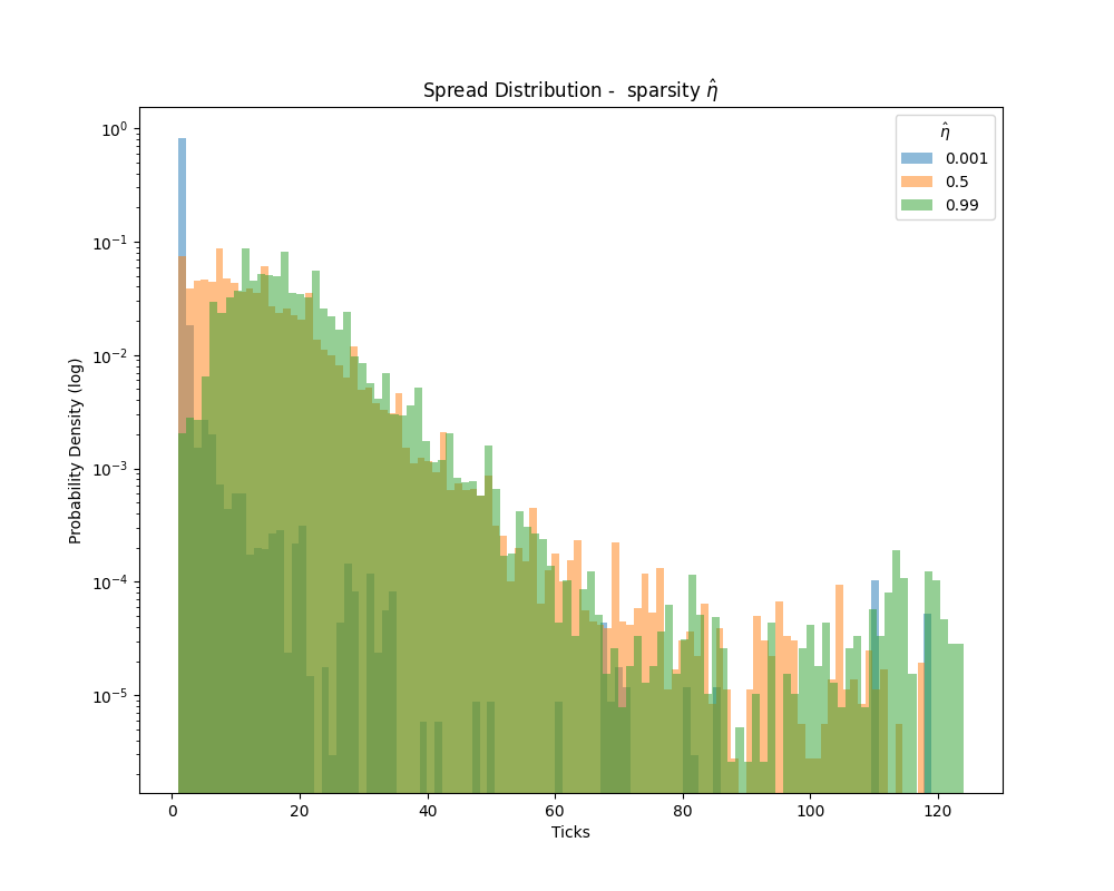
(a) Spread Distribution: Varying dynamic sparsity in the simulations

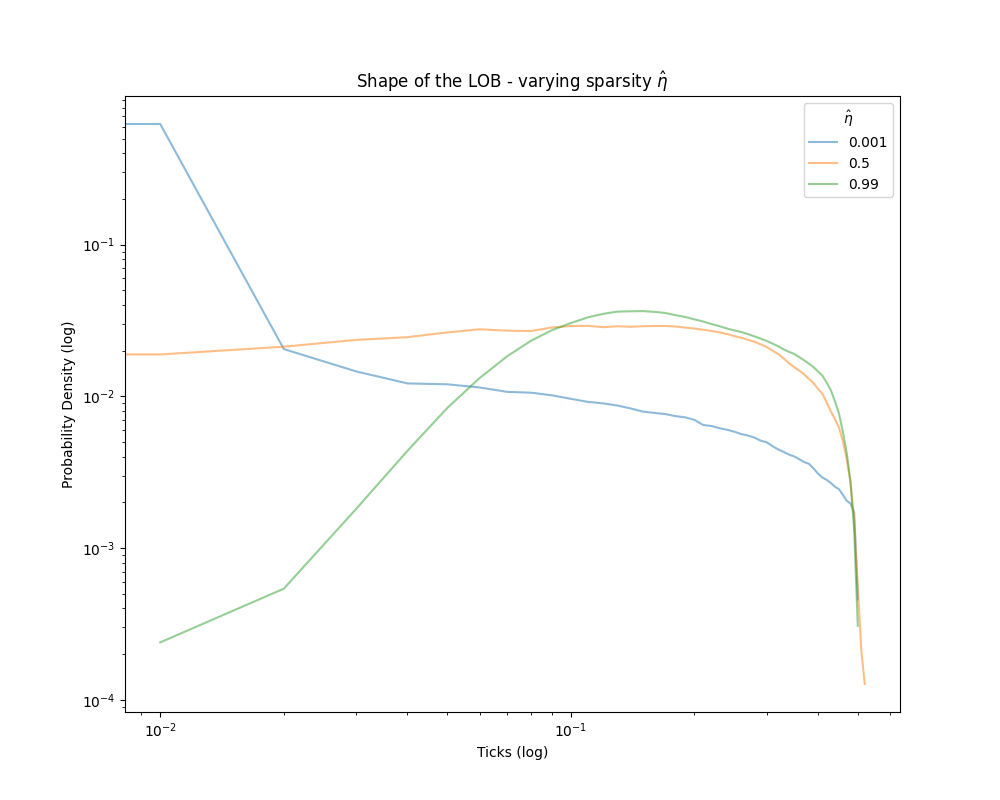
(b) Shape of the LOB: Varying dynamic sparsity in the simulations

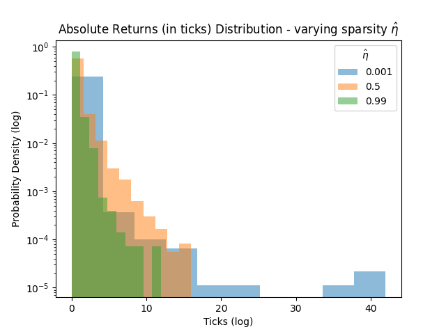
(c) Absolute Returns: Varying dynamic sparsity in the simulations

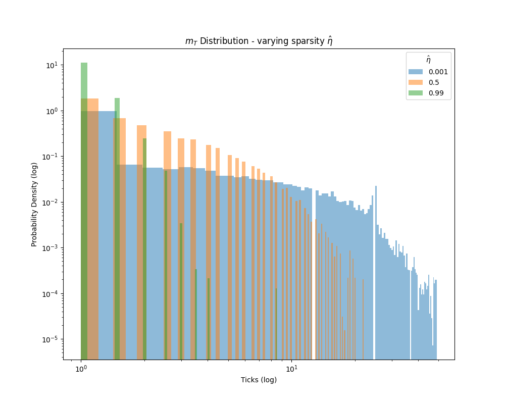
(d) Distance between top and top + 1: Varying dynamic sparsity in the simulations

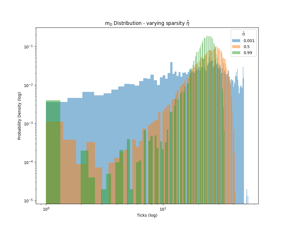
(e) $m_{D}$: Varying dynamic sparsity in the simulations

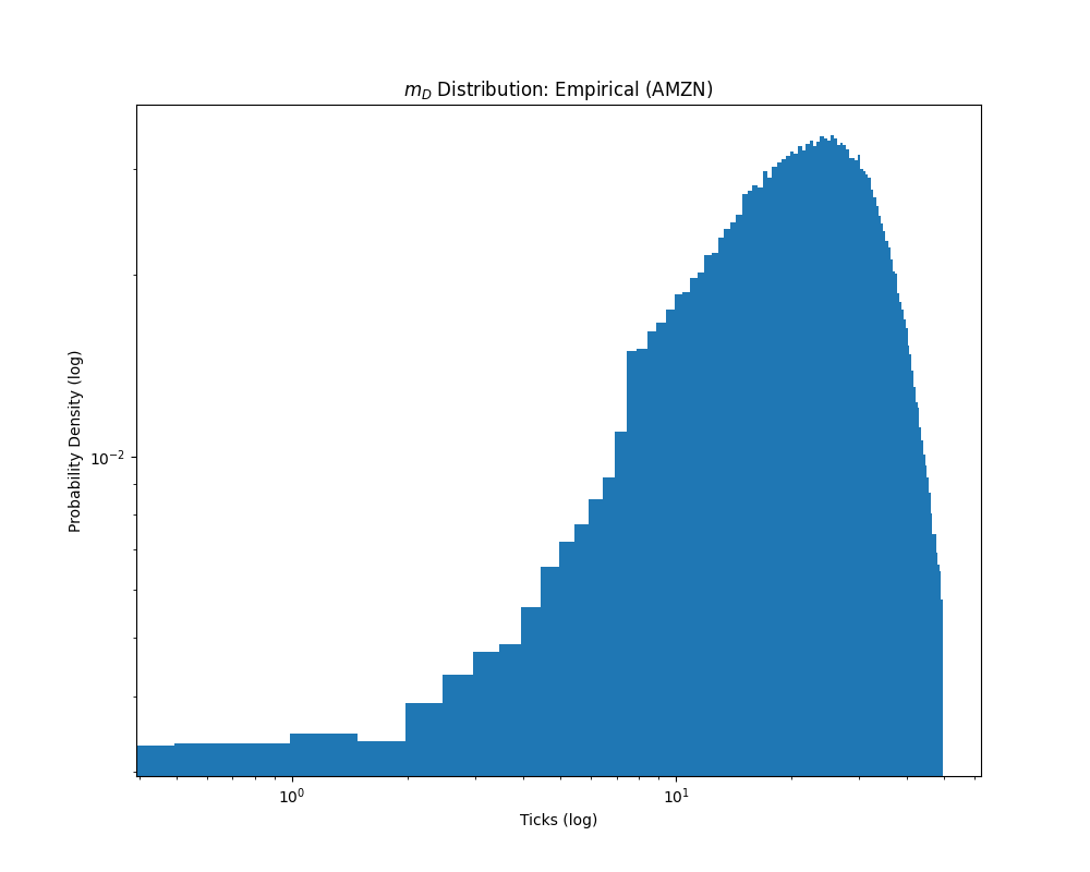
(f) $m_{D}$: AMZN Empirical

Figure 16: Simulation Study (Part 3): In this set of figures we vary the dynamic sparsity parameters $\hat{\eta}_{(.)}$, while setting the $\alpha,\beta$ parameters to a small tick stock’s setting, and observe the simulated LOB dynamics. We can see that varying the dynamic sparsity can also enable us to vary the spread distribution’s mode, the shape of the book’s maxima, the returns distributions’ tail as well as the state variables’ ($m_{T}(t),m_{D}(t)$) distribution. For empirical shapes of $m_{T}(t)$, we refer to the figure 7(a) and we show an example small tick empirical distribution for $m_{D}(t)$ in (f).

5.3 Poisson Process:

Keeping all else the same as in Section 5.1, we change the point process of the 12 events from a Hawkes Process to a Poisson Process with in-spread intensities again depend on the current spread as a power law (a similar comparison was performed in [16]). We compare the stylized facts for a small tick stock parameter setting between the Hawkes model proposed above and the Poisson model.

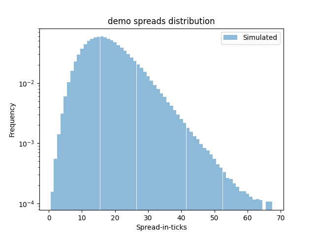
(a) Hawkes Process: Spread Distribution

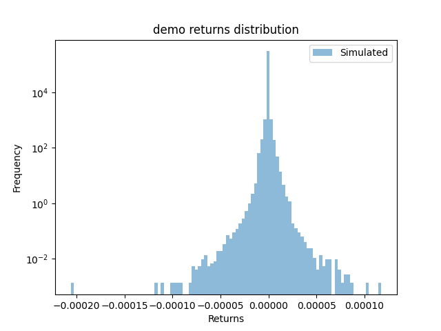
(b) Hawkes Process: Returns Distribution

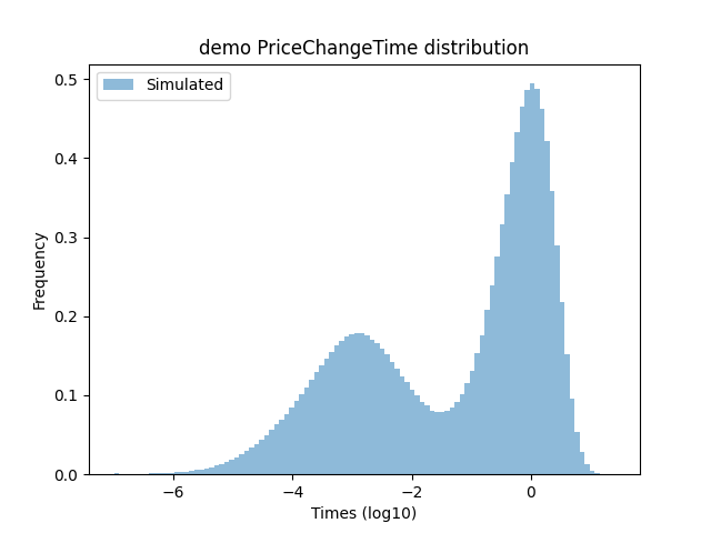
(c) Hawkes Process: PriceChangeTime Distribution

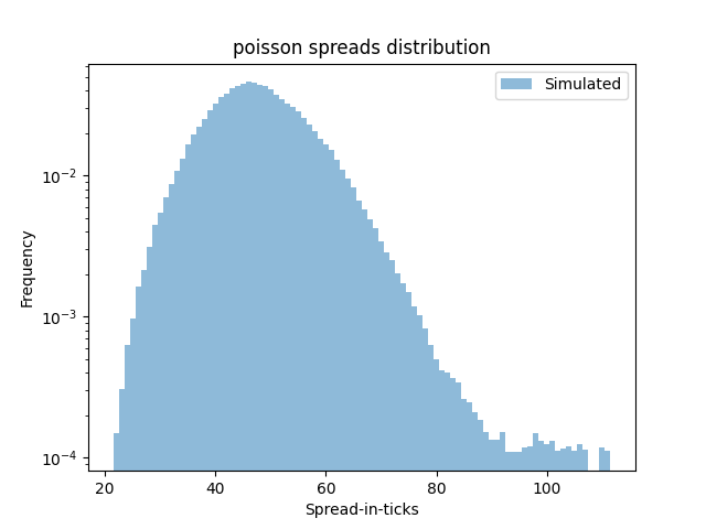
(d) Poisson Process: Spread Distribution

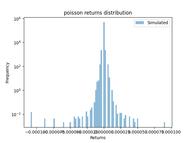
(e) Poisson Process: Returns Distribution

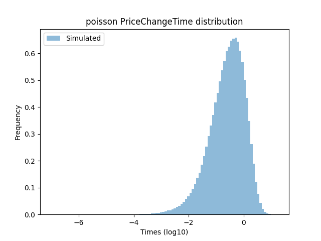
(f) Poisson Process: PriceChangeTime Distribution

Figure 17: Hawkes Process vs Poisson Process: To compare with a simpler baseline, we make use of the Poisson Process (with similar handling of IS intensities as the Hawkes Process). While the spread distribution between the two look similar in shape, the returns distribution does not. Clearly the Hawkes Process simulations have a fatter tail than the Poisson Process. Secondly, we make use of an event ‘PriceChangeTime’ which is not explicitly modelled. Here we can see clearly that the Hawkes Process is able to create a bimodal distribution of inter-event times while the Poisson distribution remains multimodal. As noted in [16], the former is more inline with empirical data as it captures the high frequency domain of the inter-event durations.

As we can see in 17, with the methodology proposed above, one can replicate the spread distribution of a small tick stock even with a Poisson model of the events’ dynamics. However we note that the distribution shape and tail of returns in the Hawkes Process model is significantly different from that of the Poisson model. We also note that while the distribution of Price Change Time (defined as the time between too successive mid price changes) is bimodal in the Hawkes Process, it is unimodal in the Poisson Process. This quantity is of interest here since we do not explicitly model this event in the point process. As noted in [16], the shape of returns and price change time distributions in the Hawkes Process method is closer to the empirical distribution shape than the Poisson Process method’s.

6 Assumptions and (Counter-) Evidence:

We make the following assumptions in this model and provide evidence for or against this assumption.

Assumption 1.

Hawkes Parameters ($\alpha,\beta,\mu^{(.)},\phi^{(.)}(t)$) and the LOB variables (i.e. LOB state variables ($m^{(.)}_{(.)}(t),Q^{(.)}_{(.)}(t)$), order sizes ($\kappa_{(.)}$), and order arrival distances from top ($\eta_{(.)}$)) are independent of each other.

We check the dependence of the LOB state variables to the events’ likelihood of occurrence by plotting the ratio of the joint probability of an event happening with the LOB state variable $v$ i.e. $P(e,v)$ with the product of the individual unconditional probabilities i.e. $P(e)P(v)$, against various categories of the width variable. This ratio informs us whether the two random variables are independent or not.

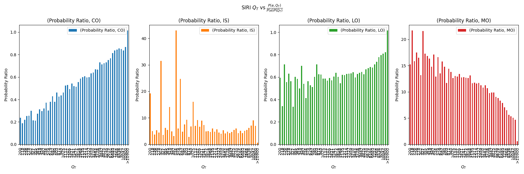
(a) SIRI $Q_{T}$

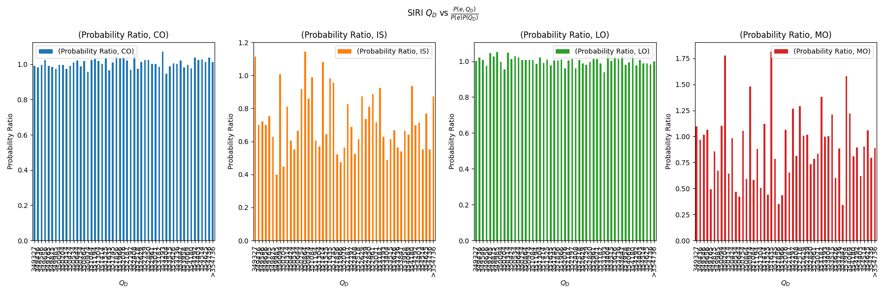
(b) SIRI $Q_{D}$

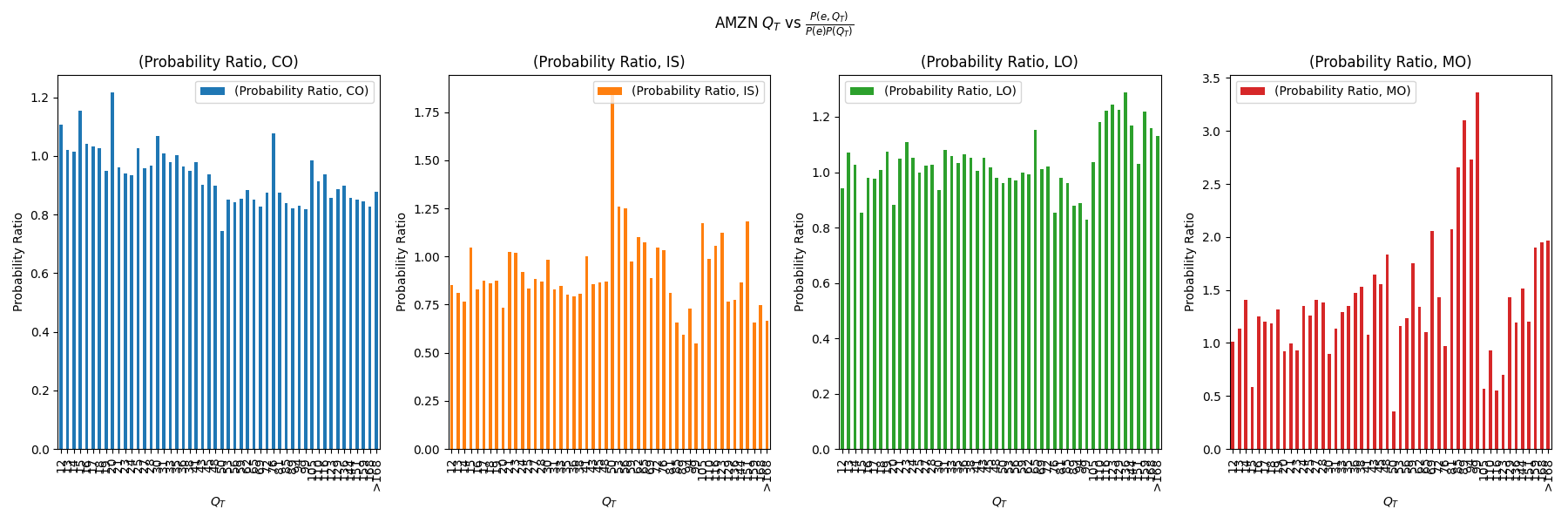
(c) AMZN $Q_{T}$

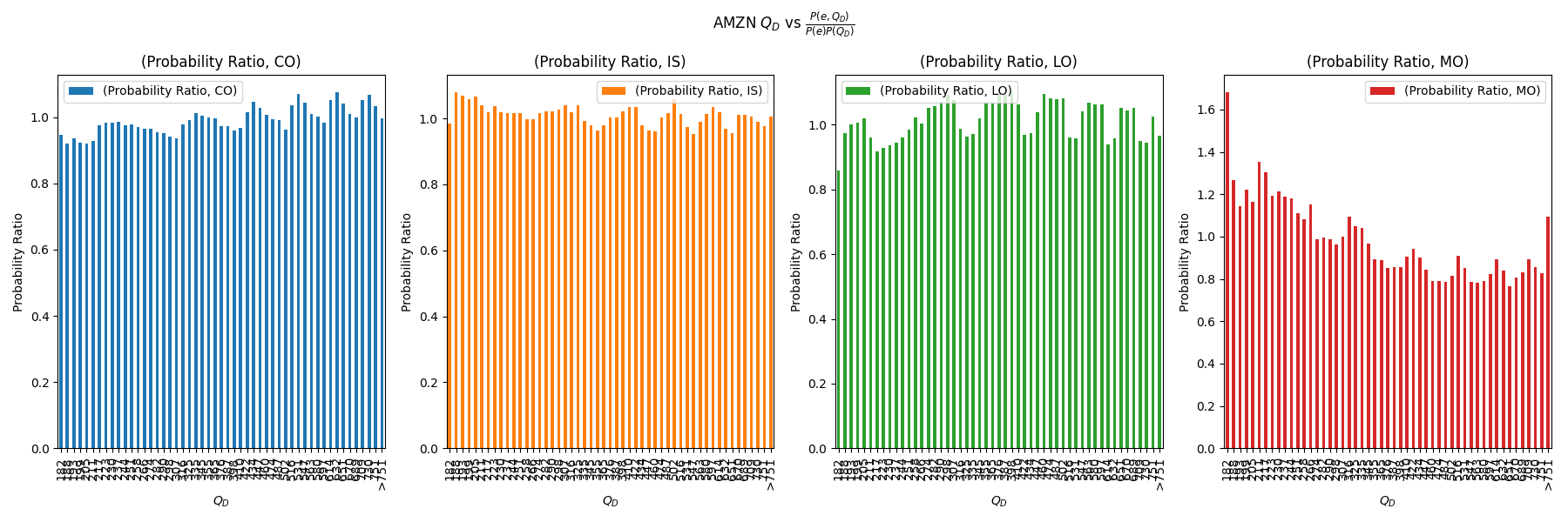
(d) AMZN $Q_{D}$

Figure 19: Testing Assumption 1: Queue Reactiveness: This independence test shows that for large tick stocks like SIRI, the intensity of events like COs, LOs and MOs, and the queue sizes at the top of the book are not independent variables. Unsurprisingly, the same is not true for the deeper volumes in a large tick LOB. For a small tick asset like AMZN, the picture becomes less clear for $Q_{T}$ however for MOs, one can observe a clear dependence among the variables. For $Q_{D}$ too we note that the MOs intensity is quite clearly not independent in the case of small tick stocks.

Queue reactiveness in the LOB has been relatively well established in point process simulations literature ([22], [24], [15]). It is evident from these papers that the intensities of LOB events depend on the current queue sizes of the LOB. However, it is unclear whether the number of past events alone (i.e., without considering individual quantities) is a reasonable proxy for the cause of this dependence. We would like to note that the Hawkes Process methodology implicitly makes the intensity depend on the count of past events. We perform tests on this assumption in Figure 19. We note that the queue reactiveness is very evident for top of the book queue size in large tick stocks however this reactiveness dies to a significant extent in small tick names. Unsurprisingly, large tick stocks dynamics seem to be unreactive to the deeper quoted volumes but there is a definite structure, particularly in MOs, for small tick stocks.

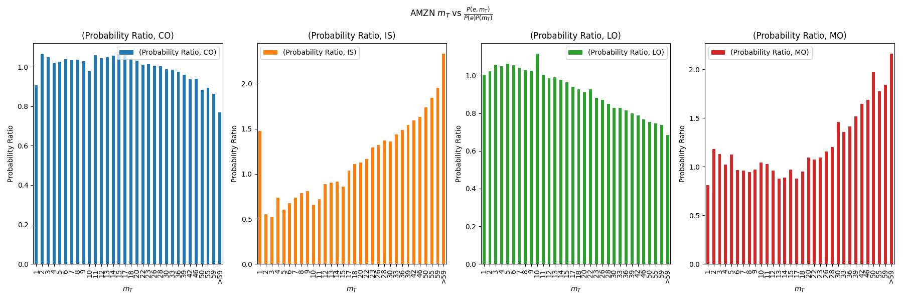
(a) $m_{T}$

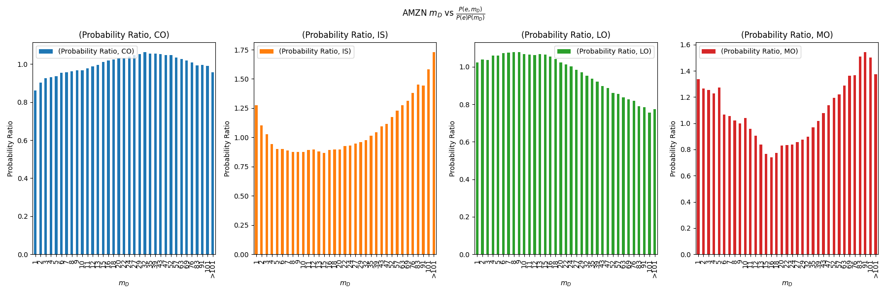
(b) $m_{D}$

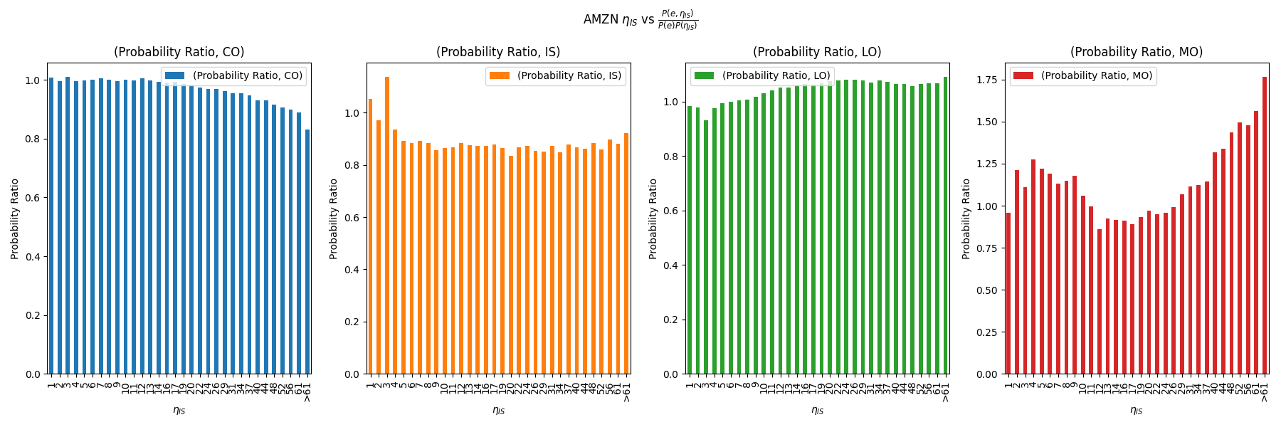
(c) $\eta_{IS}$

Figure 20: AMZN: Testing Assumption 1: We do the same analysis for a small tick stock AMZN to check the dependence between the state variables and the intensity of various events. It is evident from figures (a) and (b), that all the order intensities are related to the current width of the top queue ($m_{T}(t)$) as well as the deeper queue ($m_{D}(t)$). However for the dynamic sparsity variable, we note that there seems to be a lot of evidence (except for when $\eta_{IS}$ is very large which is a low probability event) for independence between the intensity and the previous $\eta_{IS}$ which is the most recent price improvement (in ticks) made by an in-spread LO.

Clearly from Figure 20(a), we can see that events of the type IS, CO and MO have a definitive trend with increasing $m_{T}$. While in Figure 20(b), there is a U-shape observed in IS and MO order types. Finally in Figure 20(c), we can observe a strong dependence of MO’s probability with increasing $\eta_{IS}$. However we must note that the trend becomes significant only in the right tail of the quantities which are low probability states. We do not see any clear trend when we do the same analysis for $\kappa_{LO},\kappa_{MO}$ (not illustrated). We observe similar characteristics in medium tick stocks and all other small tick stocks as well. Therefore we conclude that though for LOs and COs, we can assume the LOB state variables to be independent of their intensity functions, there exists a clear dependence of intensities of in-spread orders on the current $m_{T},m_{D}$.

Assumption 2.

Order sizes are i.i.d.

Assumption 3.

Order arrival distances from top are i.i.d.

Assumption 4.

Unseen Queue sizes on queue depletion are i.i.d.

To test the i.i.d. assumption, we measure the autocorrelations at various lags of the timeseries of the quantity. It is clear from Figure 18 that Assumption 2 is clearly violated by the empirical data. Assumption 3, however, seems to have some support from the data since the autocorrelations are absent. With regards to Assumption 4, we note that this is a modelling choice.

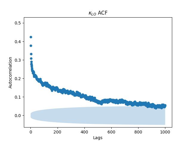
(a) $\kappa_{LO}$

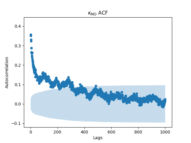
(b) $\kappa_{MO}$

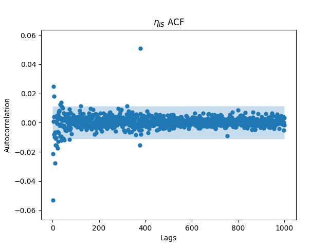
(c) $\eta_{IS}$

Figure 18: CHTR: Testing Assumption 2,3 and 4 - Clearly the ACF of order sizes ($\kappa_{(.)}$) is non neglible for 10s of lags which means that the order sizes are probably not i.i.d. However we do see the ACF of price improvements by IS orders ($\eta_{IS}$) quickly dying down to 0, giving some support to the assumption 3.

7 Discussion and Conclusion

This paper focuses on the disparity between the microstructural behaviour of the LOB between various relative tick-sizes. Tick-sizes not only define the granularity of the price formation process but also impact the market agents’ behaviour. One of our key contributions is to highlight several stylized facts, which are then used to differentiate between large, medium and small tick stocks, and define clear metrics to measure them. We also provide a set of cross-asset visualizations of the stylized facts and show how different (or similar) these attributes are with varying relative tick-size. We make use of a stylized fact known as leverage to model the LOB as a Hawkes Process with the top of the book as a separate dimension and the rest of the book (upto the median of the volume shape of the book) as a separate dimension. We then propose a simple model extending the one proposed in [16] to account for sparsity, multi-tick level price moves and the humped shape of the book for small-tick stocks. We showcase the universality of the model by performing several simulation studies using randomised parameters in the model. Thereafter, we identify the in-spread Hawkes Parameters and the sparsity variables as the critical variables which define if the simulated LOB will be similar to a large-tick or a small-tick stock. We perform several tests to showcase that a number of stylized facts like sparsity, shape, and relative returns’ distribution can be varied smoothly from that of a large-tick to small-tick asset using our model. We also compare our model’s stylized facts to that of a similar Poisson Process model where we find that the Hawkes model is superior to the Poisson one. Finally, we make note of the assumptions in this simple model and showcase a set of attributes which tests these assumptions. We show that almost all of the model’s assumptions are violated in the real data and conclude by proposing questions for further research in this area in this following.

1. Is there a mathematically tractable way of incorporating the relationship between queue sizes, width of the top of the book and width of the deeper part of the book, and the order arrival rates’ dynamics?

2. How to model order sizes such that their correlation structure observed in empirical data is preserved?

3. How can we calibrate the models above in (i) to a reasonable level of uncertainty in the model parameters?

Building on these foundations, future research will aim to enhance the adaptability and accuracy of models, leading to more robust and practical applications in limit order book modeling.

Disclaimer

Opinions and estimates constitute our judgement as of the date of this Material, are for informational purposes only and are subject to change without notice. This Material is not the product of J.P. Morgan’s Research Department and therefore, has not been prepared in accordance with legal requirements to promote the independence of research, including but not limited to, the prohibition on the dealing ahead of the dissemination of investment research. This Material is not intended as research, a recommendation, advice, offer or solicitation for the purchase or sale of any financial product or service, or to be used in any way for evaluating the merits of participating in any transaction. It is not a research report and is not intended as such. Past performance is not indicative of future results. Please consult your own advisors regarding legal, tax, accounting or any other aspects including suitability implications for your particular circumstances. J.P. Morgan disclaims any responsibility or liability whatsoever for the quality, accuracy or completeness of the information herein, and for any reliance on, or use of this material in any way.

Important disclosures at: www.jpmorgan.com/disclosures

Disclosure Statement

No potential conflict of interest was reported by the author(s).

Funding

This work was supported by JP Morgan Chase & Co.

Appendix A Stylized Facts Visualisations (continued):

In Figure 21, we show the empirical distribution of three stocks: INTC, AAPL, and AMZN, resp. a large, medium and small tick stock. We also report the time-of-day dynamics of the spread noting the ‘tick-constrained’ behaviour in INTC (and other large tick stocks). This is a common term used by practitioners to denote the fact that except for the opening hour, the spread of large tick stocks is constrained to its minimum i.e. one tick.

In Figure 22, we showcase the distance between two successive best quotes for the top 10 quotes in SIRI, PM and BKNG which is resp. a large, medium and small tick stock. We conclude that distribution of empty levels is similar across all depths and it becomes flatter as we decrease the rel. tick-size.

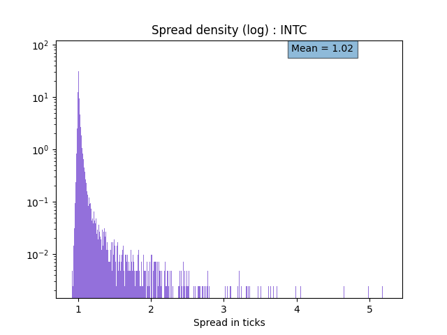
(a) INTC (Large tick) - PDF Log

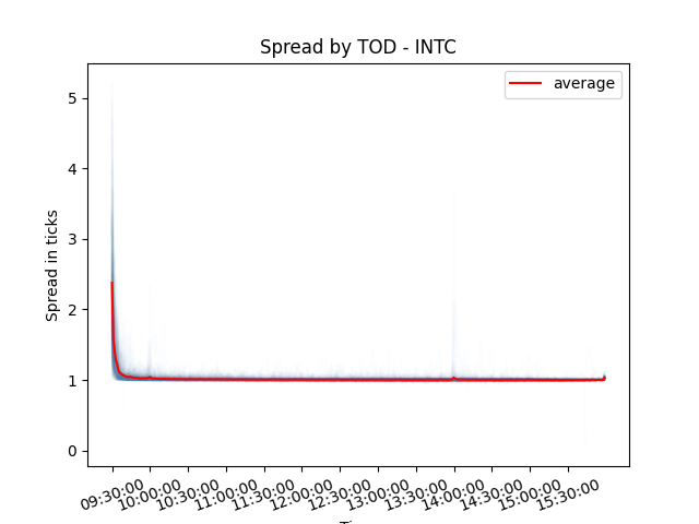
(b) INTC (Large tick) - Mean by TOD

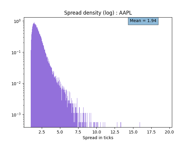
(c) AAPL (Medium tick) - PDF Log

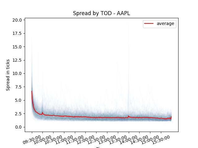
(d) AAPL (Medium tick) - Mean by TOD

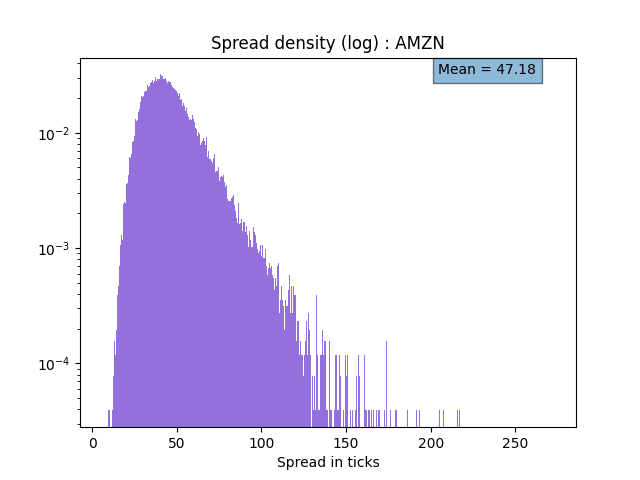
(e) AMZN (Small tick) - PDF Log

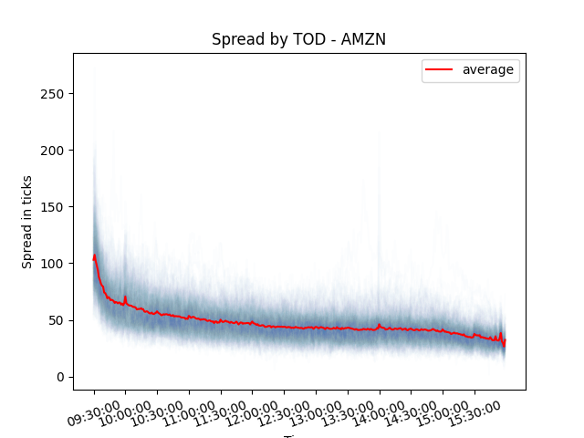
(f) AMZN (Small tick) - Mean by TOD

Figure 21: Bid-Ask Spread

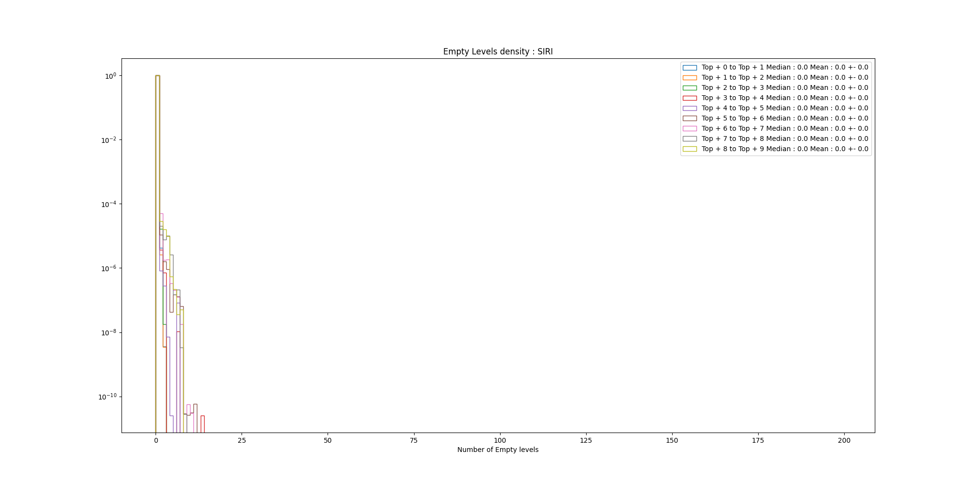
(a) SIRI (Large tick)

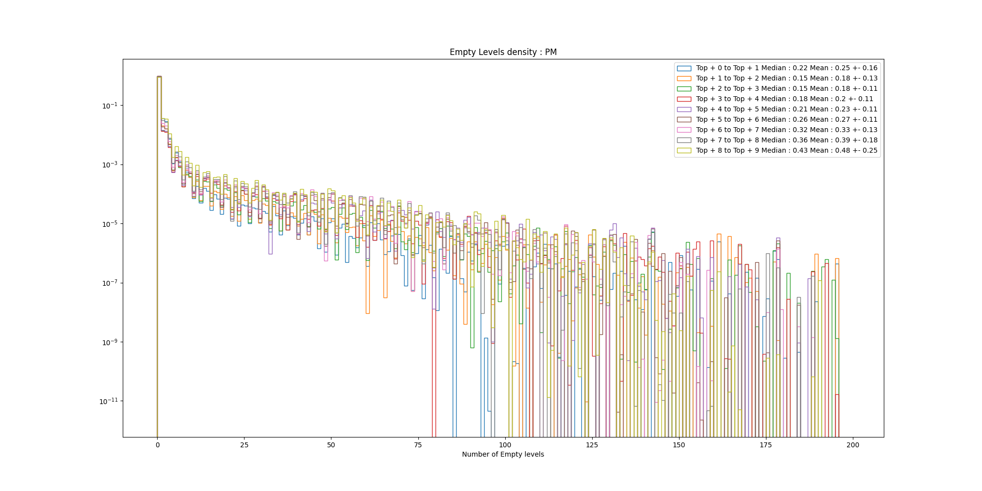
(b) PM (Medium tick)

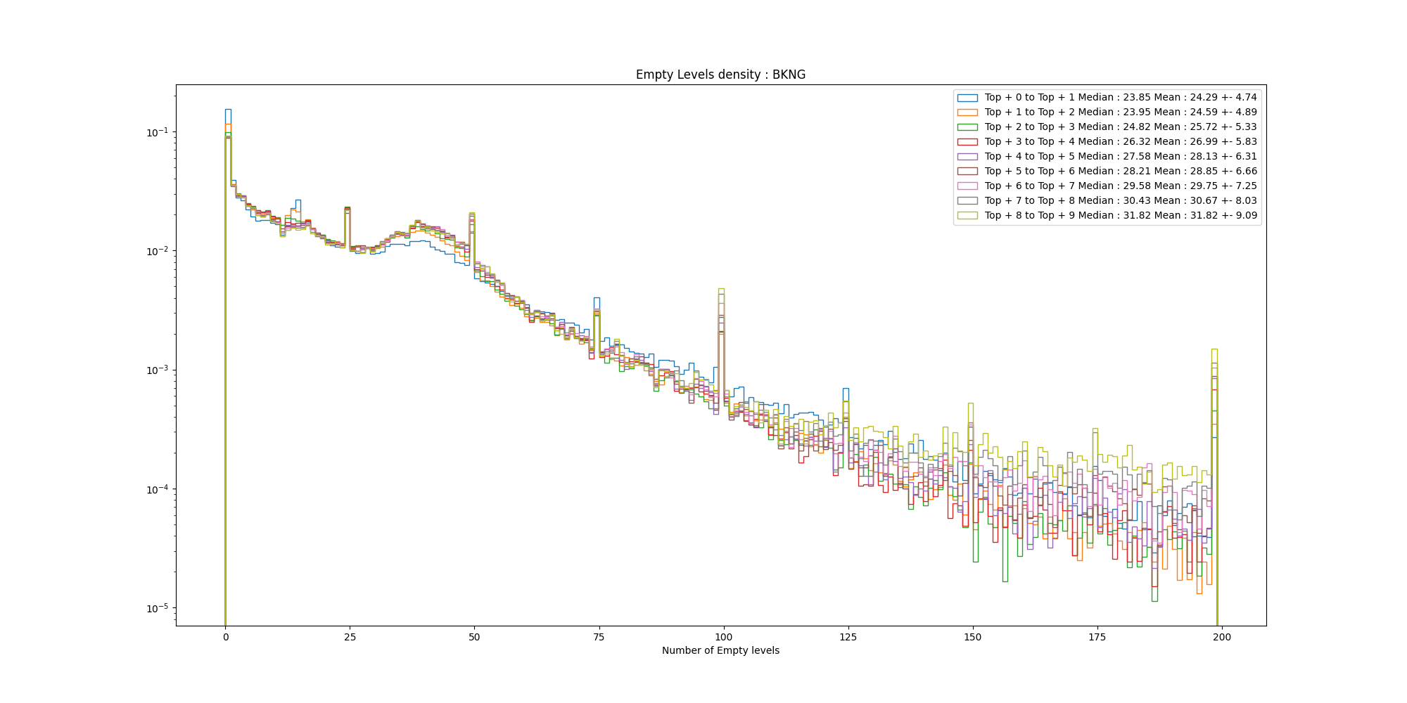
(c) BKNG (Small tick)

Figure 22: Per-stock Sparsity of the LOB : Instantaneous number of empty levels (in $) Histogram (time weighted)

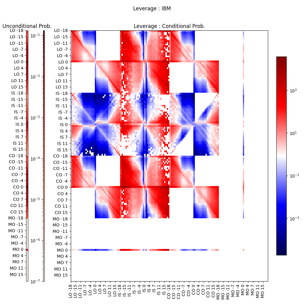
(a) IBM (Medium tick)

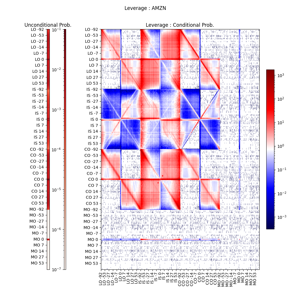
(b) AMZN (Small tick)

Figure 24: Leverage (from top): Darker the hue, more the leverage

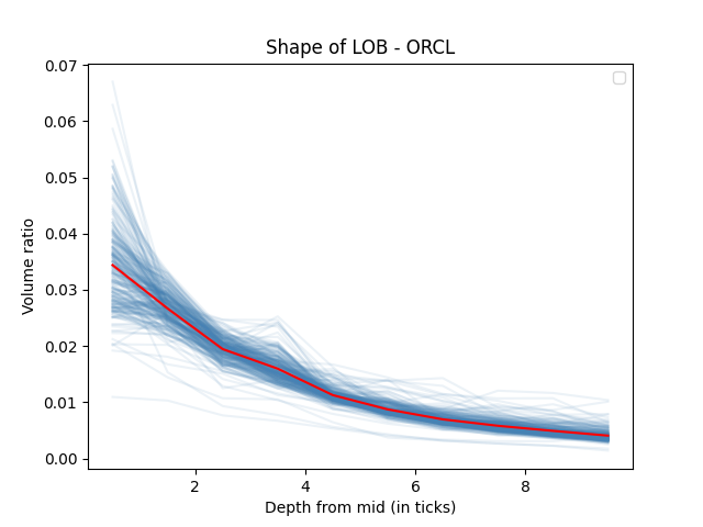
(a) ORCL (Large tick)

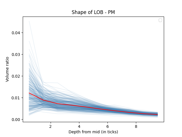
(b) PM (Medium tick)

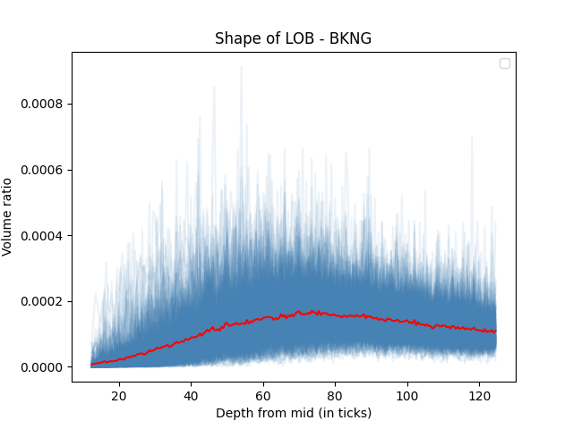
(c) BKNG (Small tick)

Figure 25: Per-stock Shape of the LOB: light blue lines are per day shapes and red is the average shape across one calendar year

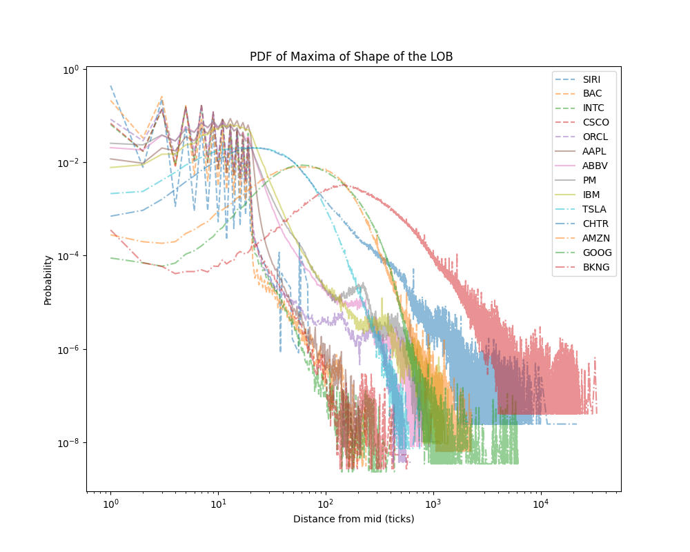
Figure 26: Distribution of Shape Maxima (log-log)

In Figure 24, we continue the depiction from Section 3.5 of uniformity of leverage across all stocks albeit with different scaling.

Figure 25, we show per stock year wide average shapes (in red) as well as daily average shapes (in light blue). Firstly the shape is stable across the whole dataset i.e. for the whole year. Secondly, we again stress the point made in Section 3.3 that the shape transforms from a decaying shape for large and medium tick stocks to that where the maxima is actually deeper in the book for small tick stocks. The distribution of this maxima’s instantaneous value is also shown in Figure 26.

Appendix B Simulation Study Results (continued):

Event	Exogenous Intensity (in events per second)
$LO_{\text{Ask}_{D}}$	0.86
$CO_{\text{Ask}_{D}}$	0.32
$LO_{\text{Ask}_{T}}$	0.33
$CO_{\text{Ask}_{T}}$	0.48
$MO_{\text{Ask}}$	0.02
$LO_{\text{Ask}_{IS}}$	0.47
$LO_{\text{Bid}_{IS}}$	0.47
$MO_{\text{Bid}}$	0.02
$CO_{\text{Bid}_{T}}$	0.48
$LO_{\text{Bid}_{T}}$	0.33
$CO_{\text{Bid}_{D}}$	0.32
$LO_{\text{Bid}_{D}}$	0.86

Table 3: Exogenous Intensity

In Table 3, we provide the exogenous intensity part of the Hawkes Process parameters ($\mu^{(.)}$) and in Figure 27, we depict the Kernel Norm matrix according to standard research practice ([3, 16]). Since the number of parameters is quite large (3 $\times$ 72 for the 72 power law kernels), we do not report them in detail.

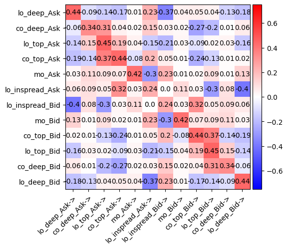
Figure 27: Norms of Kernel: AMZN.OQ

References

- [1] Frédéric Abergel et al. “Limit Order Books”, Physics of Society: Econophysics and Sociophysics Cambridge University Press, 2016 DOI: 10.1017/CBO9781316683040
- [2] Frédéric Abergel and Aymen Jedidi “Long-Time Behavior of a Hawkes Process–Based Limit Order Book” In SIAM Journal on Financial Mathematics 6.1, 2015, pp. 1026–1043 DOI: 10.1137/15M1011469
- [3] Emmanuel Bacry, Thibault Jaisson and Jean–François Muzy “Estimation of slowly decreasing hawkes kernels: application to high-frequency order book dynamics” In Quantitative Finance 16.8 Taylor & Francis, 2016, pp. 1179–1201
- [4] Emmanuel Bacry, Iacopo Mastromatteo and Jean-François Muzy “Hawkes Processes in Finance” In Market Microstructure and Liquidity 01.01, 2015, pp. 1550005 DOI: 10.1142/S2382626615500057
- [5] Jean-Philippe Bouchaud, Julius Bonart, Jonathan Donier and Martin Gould “Trades, quotes and prices: financial markets under the microscope” Cambridge University Press, 2018
- [6] Antonio Briola, Silvia Bartolucci and Tomaso Aste “Deep Limit Order Book Forecasting” In arXiv preprint arXiv:2403.09267, 2024
- [7] Antonio Briola, Silvia Bartolucci and Tomaso Aste “HLOB–Information Persistence and Structure in Limit Order Books” In arXiv preprint arXiv:2405.18938, 2024
- [8] A. Cohen “Maximum Likelihood Estimation in the Weibull Distribution Based on Complete and on Censored Samples” In Technometrics 7.4 [Taylor & Francis, Ltd., American Statistical Association, American Society for Quality], 1965, pp. 579–588 URL: http://www.jstor.org/stable/1266397
- [9] Rama Cont “Statistical Modeling of High-Frequency Financial Data” In IEEE Signal Processing Magazine 28.5, 2011, pp. 16–25 DOI: 10.1109/MSP.2011.941548
- [10] Rama Cont and Marvin S Müller “A stochastic partial differential equation model for limit order book dynamics” In SIAM Journal on Financial Mathematics 12.2 SIAM, 2021, pp. 744–787
- [11] José Da Fonseca and Riadh Zaatour “Hawkes Process: Fast Calibration, Application to Trade Clustering, and Diffusive Limit” In Journal of Futures Markets 34.6, 2014, pp. 548–579 DOI: https://doi.org/10.1002/fut.21644
- [12] Martin D. Gould et al. “Limit order books” In Quantitative Finance 13.11, 2013, pp. 1709–1742 DOI: 10.1080/14697688.2013.803
- [13] Alan G. Hawkes “Hawkes processes and their applications to finance: a review” In Quantitative Finance 18.2 Routledge, 2018, pp. 193–198 DOI: 10.1080/14697688.2017.1403131
- [14] Ulrich Horst and Wei Xu “A scaling limit for limit order books driven by Hawkes processes” In SIAM Journal on Financial Mathematics 10.2 SIAM, 2019, pp. 350–393
- [15] Weibing Huang, Charles-Albert Lehalle and Mathieu Rosenbaum “Simulating and Analyzing Order Book Data: The Queue-Reactive Model” In Journal of the American Statistical Association 110.509 [American Statistical Association, Taylor & Francis, Ltd.], 2015, pp. 107–122 URL: http://www.jstor.org/stable/24739291
- [16] Konark Jain, Nick Firoozye, Jonathan Kochems and Philip Treleaven “Limit Order Book dynamics and order size modelling using Compound Hawkes Process” In Finance Research Letters 69, 2024, pp. 106157 DOI: https://doi.org/10.1016/j.frl.2024.106157
- [17] Konark Jain, Nick Firoozye, Jonathan Kochems and Philip Treleaven “Limit Order Book Simulations: A Review” In arXiv preprint arXiv:2402.17359, 2024
- [18] Matthias Kirchner “An estimation procedure for the Hawkes process” In Quantitative Finance 17.4 Taylor & Francis, 2017, pp. 571–595
- [19] Gabriele La Spada, J. Doyne Farmer and Fabrizio Lillo “Tick Size and Price Diffusion” In Econophysics of Order-driven Markets: Proceedings of Econophys-Kolkata V Milano: Springer Milan, 2011, pp. 173–187 DOI: 10.1007/978-88-470-1766-5˙12
- [20] “LOBSTER: Limit Order Book System - The Efficient Reconstructor” Accessed: 2024-09-12, http://LOBSTER.wiwi.hu-berlin.de
- [21] Xiaofei Lu and Frédéric Abergel “High-dimensional Hawkes processes for limit order books: modelling, empirical analysis and numerical calibration” In Quantitative Finance 18.2 Routledge, 2018, pp. 249–264 DOI: 10.1080/14697688.2017.1403142
- [22] Maxime Morariu-Patrichi and Mikko S Pakkanen “State-dependent Hawkes processes and their application to limit order book modelling” In Quantitative Finance 22.3 Taylor & Francis, 2022, pp. 563–583
- [23] Ioane Muni Toke “” Market making” behaviour in an order book model and its impact on the bid-ask spread” In arXiv preprint arXiv:1003.3796, 2010
- [24] Peng Wu, Marcello Rambaldi, Jean-François Muzy and Emmanuel Bacry “Queue-reactive Hawkes models for the order flow” In arXiv preprint arXiv:1901.08938, 2019