Metric Dimension of Villarceau Grids

Abstract

The metric dimension of a graph measures how uniquely vertices may be identified using a set of landmark vertices. This concept is frequently used in the study of network architecture, location-based problems and communication. Given a graph $G$, the metric dimension, denoted as $\dim(G)$, is the minimum size of a resolving set, a subset of vertices such that for every pair of vertices in $G$, there exists a vertex in the resolving set whose shortest path distance to the two vertices is different. This subset of vertices helps to uniquely determine the location of other vertices in the graph. A basis is a resolving set with a least cardinality. Finding a basis is a problem with practical applications in network design, where it is important to efficiently locate and identify nodes based on a limited set of reference points. The Cartesian product of $P_{m}$ and $P_{n}$ is the grid network in network science. In this paper, we investigate two novel types of grids in network science: the Villarceau grid Type I and Type II. For each of these grid types, we find the precise metric dimension.

Keywords:  Villarceau grid; resolving set; basis; metric dimension
AMS Subject Classifications: 05C12

1 Introduction

Graphs are widely used to model relationships between different entities and play a fundamental role in various disciplines, including computer science, operations research and biology. Let $G$ be a connected graph having vertex set $V(G)$. For $r>0$ and $s\in V(G)$, $N_{r}(s)$ denotes the set of vertices of $G$ that are at distance $r$ from $s$. The metric dimension provides a quantitative measure of how effectively a set of vertices can function as landmarks to uniquely determine the location or identity of other vertices in the graph.

$$\mathscr{C}_{\mathscr{R}}(s)=(d(s,r_{1}),d(s,r_{2}),\ldots,d(s,r_{l}))$$

is the $l$-vector that represents the code of $s\in V(G)$ with respect to $\mathscr{R}=\{r_{1},r_{2},\ldots,r_{l}\}$. The set $\mathscr{R}$ is a resolving set for $G$ if different vertices of $G$ have distinct codes with regard to $\mathscr{R}$. The lowest cardinality of a resolving set for $G$ is denoted as $\dim(G)$, the resolving number or dimension. This idea has been significantly explored in combinatorics and numerous computer science applications. This graph’s dimension is a fundamental parameter that measures the bare minimum of vertices required to uniquely determine the position of every other vertex in the graph, according to their distances to a selected set of reference vertices.
This parameter is used in diverse domains, including robotic navigation [1], chemistry [2, 3], image processing, pattern recognition[4], linked joins in graphs [5], geometrical routing protocols [6, 4, 7] and network intruder detection[8]. Numerous intriguing similarities between the coin weighing and mastermind game have been demonstrated in [9, 10]. Practical scenarios often employ heuristics and approximation algorithms to determine or estimate this parameter in practical scenarios.
This investigation traces back to the early 1970s, with one of the seminal papers by Harary and Melter [11] in 1976, motivated by challenges in chemical graph theory and communication networks. Initially introduced by Slater in graphs, the concept gained more attention as researchers explored its properties and applications. As soon as researchers recognized the practical applications in numerous domains, there was a surge in interest in algorithmic approaches and heuristics for computing or approximating the metric dimension. Several papers during this period focused on efficient algorithms and approximation techniques.
Despite its NP-hard complexity for arbitrary graphs, significant strides have been achieved in solving the metric dimension problem for particular classes of graphs, leveraging efficient algorithms and approximation techniques. Beyond theoretical advances, practical applications of the metric dimension and its variants continue to emerge, underscoring its relevance across various disciplines.
The resolving-power domination number is examined in [12] for probabilistic neural networks, a specific type of RNN (Recurrent Neural Networks). The performance of parallel computing systems on a grand scale is significantly influenced by the quality of the interconnection networks. The various processing components that comprise up a parallel computing system rely extensively on interconnection networks to exchange data and communicate with one another. The metric size and fault tolerance of fractal cubic networks were computed by Arulperumjothi et al. [13]. An irregular network with a convex triangular metric size is computed in [14]. Prabhu et al. [15] refute the earlier findings from [16] and [17] by re-examining the metric dimension variant for butterfly networks, silicate networks, and Benes networks. Furthermore, a variety of architectures, notably generalized fat trees [18], trees [1], torus networks [19], 2-trees [20], multi-dimensional grids [1, 21], Benes networks [22], hypercube [23], honeycomb networks [25, 24], Illiac networks [26], enhanced hypercubes [27], Petersen graphs [28] and circulant graphs [29, 31, 30] have been analysed. This encompasses various types of graphs, such as Toeplitz graphs [32], infinite graphs [33], Cayley graphs [34], Kneser and Johnson graphs[35], Cartesian product graphs[10], chain graphs [36], fullerene graphs [37], Grassmann graphs[38], convex polytopes [40, 39], permutation graphs [41], bilinear graphs [42, 43], wheel-related graphs[44], incidence graph [45], regular graphs [46] and unicyclic graphs [47]. Numerous details about this topic are available in [48].
A grid is a graph having vertices $\{v_{i,j}:(i,j)\in[\![1,m]\!]\times[\![1,n]\!]\}$ and edges $\{v_{i,j}v_{i^{\prime},j^{\prime}}:|i-i^{\prime}|+|j-j^{\prime}|=1\}$. This is $m\times n$ grid, also known as Cartesian product $P_{m}\square P_{n}$ [49]. There are different grid configurations, including square, hexagonal, triangular, and rectangle ones. Because of their unique characteristics and uses, each kind of grid is appropriate for a variety of jobs and applications. Grids are a useful tool for organising data in spreadsheets, representing spatial data in geographic information systems, and providing a foundation for alignment and layout in graphic design. Mathematicians, computer scientists, and network analysts frequently utilise grid graphs to simulate spatial relationships, connectivity, and algorithms. In computer networks, grids are important because they offer an organised framework for resource management, communication, and service optimisation. Enhancing network performance, scalability, stability, and efficiency in diverse networked contexts is possible through the use of grid-based approaches and algorithms. Tomescu and Melter [4] examined the metric size for grid graphs where the distances are defined in $L_{1}$ metrics. They demonstrated that, under the $L_{1}$ metric, the metric size is two, whereas under the $L_{\infty}$ metric, it is three. Under the $L_{1}$ metric, Kuller [1] yields a characterization of the metric size of $d$-dimension. The metric basis is provided in [50] for the square grid graph. The study of graceful labelling for the grid graph has been investigated by Acharya and Gill [51]. This article examines dimensions for novel grid structures, such as the Villarceau grids.

2 Villarceau Grids

The Villarceau circles [52, 53] are a set of circles formed by the intersection of a plane inclined at a specific angle to the axis of a torus. They are named after the 19th-century French mathematician Yvon Villarceau, who studied and described these circles. When a plane intersects a torus (a surface shaped like a doughnut or a ring) at a non-perpendicular angle to the torus axis, these circles, known as the Villarceau circles, form a distinctive and captivating pattern. They are essential in understanding the geometry and topology of toroidal shapes and find applications across various mathematical and scientific disciplines. The properties of the Villarceau torus are studied in depth by Manuel [53].
The Villarceau torus is a geometric configuration that arises from the intersection of a torus with a plane at a specific inclination to the torus’s axis. It provides insights into the geometric relationships and topological properties of toroidal shapes, making it significant in geometry and topology. This mathematical concept has applications in various fields and provides a unique perspective on the interaction between planes and tori. Figure 1 illustrates the Villarceau torus, where the red and green circles, also known as the Villarceau circles, have an oblique inclination compared to the white and yellow circles of the torus. The Villarceau grids are motivated by the Villarceau torus.

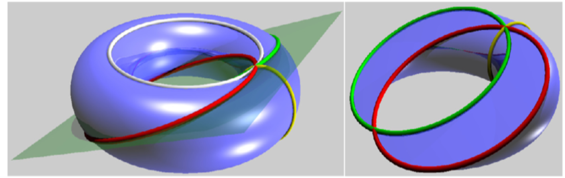
Figure 1: Villarceau torus

Our understanding of the Villarceau torus has empowered us to define the Villaceau grid, a novel grid layout distinct from traditional designs. The study of the Villarceau grid enhances our comprehension of complex geometric structures and enriches mathematical exploration.
The Villarceau grid Type I is denoted by $VG^{1}_{m,n}$, where $1\leq m\leq n$. The vertex set is defined by $\{(2i,2j+1):i\in[\![0,n]\!],j\in[\![0,m-1]\!]\}\bigcup\{(2i+1,2j):i\in[\![0,n-1]\!],j\in[\![0,m]\!]\}$ and there is an edge between $(i_{1},j_{1})$ and $(i_{2},j_{2})$ if $|i_{1}-i_{2}|=1$ and $|j_{1}-j_{2}|=1$. The notation $[\![r,s]\!]$ will be utilised for expressing the range of numbers $r<s$, $\{r,r+1,\ldots,s\}$.

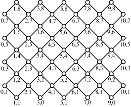
(a)

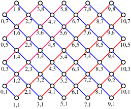
(b)

Figure 2: (a) $VG^{1}_{4,5}$; (b) Acute lines are depicted in red, while obtuse lines are depicted in blue.

The Villarceau grid Type II is denoted as $VG^{2}_{m,n}$, where $1\leq m<n$ (Figure 3). The vertex set is defined by $\{(2i+1,2j+1):i\in[\![0,n-2]\!],j\in[\![0,m-1]\!]\}\bigcup\{(2i,2j):i\in[\![0,n-1]\!],j\in[\![0,m]\!]\}$ and the vertices $(i_{1},j_{1})$ and $(i_{2},j_{2})$ are adjacent if $|i_{1}-i_{2}|=1$ and $|j_{1}-j_{2}|=1$.

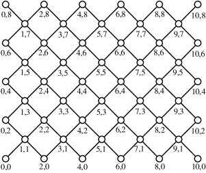
Figure 3: $VG^{2}_{4,6}$

A comparison between the standard grid and the Villarceau grid is shown in the following table.

Table 1: Grid and Villarceau grid architectures comparison

	Grid $(P_{m}\square P_{n})$	Villarceau grid Type I $(VG^{1}_{m,n})$	Villarceau grid Type II $(VG^{2}_{m,n})$
Number of vertices	$mn$	$2mn+m+n$	$2mn-m+n$
Number of edges	$2mn-m-n$	$4mn$	$4m(n-1)$
Diameter	$m+n-2$	$2n$	$2n$
Degree of vertices	$2,3,4$	$2,4$	$1,2,4$
Metric dimension	$2$	$\left\{\begin{array}[]{rll}=3&\mbox{for}\enspace n\leq 2m+1\\ >3&\mbox{for}\enspace n>2m+1\\ \end{array}\right.$	$\left\{\begin{array}[]{rll}=3&\mbox{for}\enspace n\leq 2m+1\\ >3&\mbox{for}\enspace n>2m+1\\ \end{array}\right.$
Average distance	$(m^{3}n^{2}-mn^{2}+$ $m^{2}n^{3}-m^{2}n)/$ $3(m^{2}n^{2}-mn)$	$(10n^{3}-10n+40m^{2}n^{3}+$ $40mn^{3}+60m^{2}n^{2}+30mn^{2}+$ $30m^{2}n+20m^{4}n+40m^{3}n-$ $20mn-4m^{5}+10m^{3})/$ $15(4m^{2}n^{2}+4m^{2}n+4mn^{2}+$ $m^{2}+n^{2}-m-n)$	$2(15m^{2}n+20m^{3}n+10m^{4}n-$ $2m^{5}-10m^{4}-5m^{3}-$ $20m^{3}n^{2}+5n^{3}-20m^{2}n^{2}+$ $10m^{2}-15mn^{2}+7m+$ $20n^{2}m^{3}+20n^{3}m^{2}-10n^{2}m^{2}+$ $20mn^{3}-10mn-5n)/$ $15(4m^{2}n^{2}-4m^{2}n+4mn^{2}+$ $-4mn+m^{2}+m+n^{2}-n)$

3 Main Results

Theorem 1.

[1] If a graph $G$’s metric basis is $\{s,t\}$ , then the following criteria are satisfied.

1. The vertex $s,t$ in $G$ has a degree of $3$ or less.

2. Between vertices $s$ and $t$ in $G$, there is precisely a shortest path $P$.

3. The degree of an internal vertex of $P$ in $G$ is less than or equal to $5$.

For $n=m=1$, $VG^{1}_{1,1}\cong C_{4}$ where $C_{4}$ is a cycle with 4 vertices whose metric dimension is 2, which is discussed in [1].

Lemma 2.

If $2\leq n\leq 2m+1$ and $m\neq n$, then $\dim(VG^{1}_{m,n})>2$.

Proof.

Suppose, $\dim(VG^{1}_{m,n})=2$ and $\{u,v\}$ is a resolving set of $VG^{1}_{m,n}$. By Theorem 1, there is a unique shortest $u,v$-path wherein $\deg_{G}(u)\leq 3$, $\deg_{G}(v)\leq 3$. The following cases need to be explored:
Case 1: $u$ and $v$ are on a same boundary. As there are four boundaries, We have four subcases as follows:
Case 1.1: $u=(2t+1,0)$ and $v=(2t+3,0)$, $t\in[\![0,n-2]\!].$
Then $d(u,(2t+1,2))=d(v,(2t+1,2))$ and $d(u,(2t+3,2))=d(v,(2t+3,2))$, a contradiction.
Case 1.2: $u=(0,2t+1)$ and $v=(0,2t+3)$, $t\in[\![0,m-2]\!].$
Then $d(u,(2,2t+1))=d(v,(2,2t+1))$ and $d(u,(2,2t+3))=d(v,(2,2t+3))$, a contradiction.
Case 1.3: $u=(2t+1,2m)$ and $v=(2t+3,2m)$, $t\in[\![0,n-2]\!].$
We get $d(u,(2t+1,2m-2))=d(v,(2t+1,2m-2))$ and $d(u,(2t+3,2m-2))=d(v,(2t+3,2m-2))$, a contradiction.
Case 1.4: $u=(2n,2t+1)$ and $v=(2n,2t+3)$, $t\in[\![0,m-2]\!].$
We have $d(u,(2n-2,2t+1))=d(v,(2n-2,2t+1))$ and $d(u,(2n-2,2t+3))=d(v,(2n-2,2t+3))$, a contradiction.
Case 2: $u$ and $v$ are the endpoints of the same obtuse line (refer to Figure 2).
Case 2.1: $u=(2t+1,0)$ and $v=(0,2t+1)$, $t\in[\![0,m-1]\!].$
Then $d(u,(2t+3,0))=d(v,(2t+3,0))$ and $d(u,(2t+3,2))=d(v,(2t+3,2))$, a contradiction.
Case 2.2: $u=(2t+1,0)$ and $v=(2t-2m+1,2m)$, $t\in$[​[$m,n-2$]​].
We get $d(u,(2t+3,0))=d(v,(2t+3,0))$ and $d(u,(2t+3,2))=d(v,(2t+3,2))$, a contradiction.
Case 2.3: $u=(2n-1,0)$ and $v=(2n-2m-1,2m).$
Then $d(u,(2n-2m-3,2m))=d(v,(2n-2m-3,2m))$ and $d(u,(2n-2m-3,2m-2))=d(v,(2n-2m-3,2m-2))$, a contradiction.
Case 2.4: $u=(2n,2t+1)$ and $v=(2n-2m+2t+1,2m)$, $t\in[\![0,m-1]\!].$
We have $d(u,(2n-2m+2t-1,2m))=d(v,(2n-2m+2t-1,2m))$ and $d(u,(2n-2m+2t-1,2m-2))=d(v,(2n-2m+2t-1,2m-2))$, a contradiction.
Case 3: $u$ and $v$ are the endpoints of a same acute line.
Case 3.1: $u=(0,2t+1)$ and $v=(2m-2t-1,2m)$, $t\in[\![0,m-1]\!].$
Then $d(u,(2m-2t+1,2m))=d(v,(2m-2t+1,2m))$ and $d(u,(2m-2t+1,2m-2))=d(v,(2m-2t+1,2m-2))$, a contradiction.
Case 3.2: $u=(2t+1,0)$ and $v=(2m+2t+1,2m)$, $t\in[\![0,n-m-2]\!].$
We have $d(u,(2m+2t+3,2m))=d(v,(2m+2t+3,2m))$ and $d(u,(2m+2t+3,2m-2))=d(v,(2m+2t+3,2m-2))$, a contradiction.
Case 3.3: $u=(2n-1,2m)$ and $v=(2n-2m-1,0).$
We get $d(u,(2n-2m-3,0))=d(v,(2n-2m-3,0))$ and $d(u,(2n-2m-3,2))=d(v,(2n-2m-3,2))$, a contradiction.
Case 3.4: $u=(2n-2t-1,0)$ and $v=(2n,2t+1)$, $i\in[\![0,m-1]\!].$
Then $d(u,(2n-2t-3,0))=d(v,(2n-2t-3,0))$ and $d(u,(2n-2t-3,2))=d(v,(2n-2t-3,2))$, a contradiction.
Therefore, we conclude that $\dim(VG^{1}_{m,n})>2$. ∎

Lemma 3.

If $n\geq 2$ and $m=n$, then $\dim(VG^{1}_{m,n})>2$.

Proof.

Suppose, $\dim(VG^{1}_{m,n})=2$ and $\{u,v\}$ is a resolving set for $VG^{1}_{m,n}$. By Theorem 1 we consider the cases below.
Case 1: $u$ and $v$ are on a same boundary.
Case 1.1: $u=(2t+1,0)$ and $v=(2t+3,0)$, $t\in[\![0,n-2]\!].$
Then $d(u,(2t+1,2))=d(v,(2t+1,2))$ and $d(u,(2t+3,2))=d(v,(2t+3,2))$, a contradiction.
Case 1.2: $u=(0,2t+1)$ and $v=(0,2t+3)$, $t\in[\![0,m-2]\!].$
Then $d(u,(2,2t+1))=d(v,(2,2t+1))$ and $d(u,(2,2t+3))=d(v,(2,2t+3))$, a contradiction.
Case 1.3: $u=(2t+1,2m)$ and $v=(2t+3,2m)$, $t\in[\![0,n-2]\!].$
We get $d(u,(2t+1,2m-2))=d(v,(2t+1,2m-2))$ and $d(u,(2t+3,2m-2))=d(v,(2t+3,2m-2))$, a contradiction.
Case 1.4: $u=(2n,2t+1)$ and $v=(2n,2t+3)$, $t\in[\![0,m-2]\!].$
We have $d(u,(2n-2,2t+1))=d(v,(2n-2,2t+1))$ and $d(u,(2n-2,2t+3))=d(v,(2n-2,2t+3))$, a contradiction.
Case 2: $u$ and $v$ are the endpoints of the same obtuse line.
Case 2.1: $u=(2t+1,0)$ and $v=(0,2t+1)$, $t\in[\![0,m-2]\!].$
Then $d(u,(2t+3,0))=d(v,(2t+3,0))$ and $d(u,(2t+3,2))=d(v,(2t+3,2))$, a contradiction.
Case 2.2: $u=(2n+t-1,t)$ and $v=(t,2n+t-1)$, $t\in$[​[$0,1$]​].
We get $d(u,(2n+t-3,t))=d(v,(2n+t-3,t))$ and $d(u,(2n+t-1,t+2))=d(v,(2n+t-1,t+2))$, a contradiction.
Case 2.3: $u=(2n,2t+1)$ and $v=(2t+1,2m)$, $t\in[\![0,m-1]\!].$
We have $d(u,(2t-1,2m-2))=d(v,(2t-1,2m-2))$ and $d(u,(2t-1,2m))=d(v,(2t-1,2m))$, a contradiction.
Case 3: $u$ and $v$ are the endpoints of a same acute line.
Case 3.1: $u=(0,2t+1)$ and $v=(2m-2t-1,2m)$, $t\in[\![1,m-1]\!].$
Then $d(u,(2m-2t+1,2m))=d(v,(2m-2t+1,2m))$ and $d(u,(2m-2t+1,2m-2))=d(v,(2m-2t+1,2m-2))$, a contradiction.
Case 3.2: $u=(t,1-t)$ and $v=(2m+t-1,2m-t)$, $t\in[\![0,1]\!].$
We have $d(u,(t,3-t))=d(v,(t,3-t))$ and $d(u,(t+2,1-t))=d(v,(t+2,1-t))$, a contradiction.
Case 3.3: $u=(2t+1,0)$ and $v=(2m,2m-2t-1)$, $t\in[\![1,n-1]\!].$
We get $d(u,(2t-1,0))=d(v,(2t-1,0))$ and $d(u,(2t-1,2))=d(v,(2t-1,2))$, a contradiction.
Therefore, we conclude that $\dim(VG^{1}_{m,n})>2$. ∎

The highlighted points in Figure 4 are the vertices that are not resolved by these two points $(1,0)$ and $(2n-1,0)$. Also, similar representations are given in similar colours. The following lemma demonstrates the usefulness of these points.

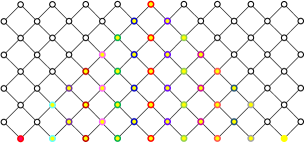
(a)

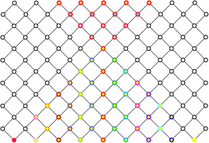
(b)

Figure 4: (a) $VG^{1}_{4,9}$; (b) $VG^{1}_{6,9}$

Lemma 4.

For the graph $VG^{1}_{m,n}$ where $2\leq n\leq 2m+1$, the intersection $N_{r_{1}}((1,0))\cap N_{r_{2}}((2n-1,0))$ is non-empty.

Proof.

Case 1: Let $r_{1}=2\nu-1$ and $r_{2}=2\gamma-1$, where $\nu,\gamma\in[\![1,n]\!].$
Case 1.1: $\nu,\gamma\in[\![1,m]\!]$.
$N_{r_{1}}((1,0))=S_{1}\cup S_{2}$, where $S_{1}=\{(2t,r_{1}):\enspace t\in[\![0,\frac{r_{1}-1}{2}]\!]$} and
$S_{2}=\{(r_{1}+1,r_{1}-2t):\enspace t\in[\![0,\frac{r_{1}-1}{2}]\!]$}
$N_{r_{2}}((2n-1,0))=S_{1}\cup S_{2}$, where $S_{1}=\{(2n-2t,r_{2}):\enspace t\in[\![0,\frac{r_{2}-1}{2}]\!]\}$ and
$S_{2}=\{(2n-r_{2}-1,r_{2}-2t):\enspace t\in[\![0,\frac{r_{2}-1}{2}]\!]\}$
Case 1.2: $\nu,\gamma\in[\![m+1,n]\!].$
$N_{r_{1}}((1,0))=\{(r_{1}+1,2m-2t+1):t\in[\![1,m]\!]\}$.
$N_{r_{2}}((2n-1,0))=\{(2n-r_{2}-1,2m-2t+1):t\in[\![1,m]\!]\}$
$N_{r_{1}}((1,0))\cap N_{r_{2}}((2n-1,0))=A\cup B$ and $r_{1}=2\nu-1$, where $\nu\in[\![2,n-2]\!]$

$$A=\left\{\begin{array}[]{ll}\{(r_{1}+1,r_{1}-2t):&t\in[\![0,\frac{r_{1}-1}{2}]\!]\},\enspace\text{if}\enspace\nu\in[\![1,\lceil\frac{n-3}{2}\rceil]\!];\enspace r_{2}=2n-r_{1}-2\\ \{(r_{1}+1,2n-r_{1}-2t-2):&t\in[\![0,\frac{2n-r_{1}-3}{2}]\!]\},\enspace\text{if}\enspace\nu\in[\![\frac{n-1}{2},n-3]\!];\enspace r_{2}=2n-r_{1}-2\\ \end{array}\right.$$

$$B=\left\{\begin{array}[]{ll}\emptyset:&n=2m+1\\ \{(2n-r_{1}+2t-1,r_{1}):&\enspace t\in[\![0,r_{1}-n+1]\!]\},\enspace\text{if}\enspace n<2m+1,\enspace\nu\in[\![\frac{n-1}{2},m-1]\!];\enspace r_{2}=r_{1}\\ \end{array}\right.$$

Case 2: $r_{1}=2\nu$ and $r_{2}=2\gamma$, where $\nu,\gamma\in[\![1,n-1]\!].$
Case 2.1: $\nu,\gamma\in[\![1,m]\!]$.
$N_{r_{1}}((1,0))=S_{1}\cup S_{2}$, where $S_{1}=\{(2t+1,r_{1}):\enspace t\in[\![0,\frac{r_{1}}{2}]\!]\}$ and
$S_{2}=\{(r_{1}+1,r_{1}-2t-2):\enspace t\in[\![0,\frac{r_{1}-2}{2}]\!]\}$
$N_{r_{2}}((2n-1,0))=S_{1}\cup S_{2}$, where $S_{1}=\{(2n-2t-1,r_{2}):\enspace t\in[\![0,\frac{r_{2}-2}{2}]\!]\}$ and
$S_{2}=\{(2n-r_{2}-1,r_{2}-2t):\enspace t\in[\![0,\frac{r_{2}}{2}]\!]\}$
Case 2.2: $\nu,\gamma\in[\![m+1,n-1]\!]$.
$N_{r_{1}}((1,0))=\{(r_{1}+1,2m-2t):t\in[\![0,m]\!]$}
$N_{r_{2}}((2n-1,0))=\{(2n-r_{2}-1,2m-2t):t\in[\![0,m]\!]\}$
$N_{r_{1}}((1,0))\cap N_{r_{2}}((2n-1,0))=A\cup B$ and $r_{1}=2\nu$, where $\nu\in[\![1,n-2]\!]$

$$A=\left\{\begin{array}[]{ll}\{(r_{1}+1,r_{1}-2t):&t\in[\![0,\frac{r_{1}}{2}]\!]\},\enspace\text{if}\enspace\nu\in[\![1,\lfloor\frac{n-1}{2}\rfloor]\!];\enspace r_{2}=2n-r_{1}-2\\ \{(r_{1}+1,2n-r_{1}-2t-2):&t\in[\![0,\frac{2n-r_{1}-2}{2}]\!]\},\enspace\text{if}\enspace\nu\in[\![\lfloor\frac{n+1}{2}\rfloor,n-2]\!];\enspace r_{2}=2n-r_{1}-2\\ \end{array}\right.$$

$$B=\left\{\begin{array}[]{ll}\emptyset:&n=2m+1\\ \{(2n-r_{1}+2t-1,r_{1}):&,\enspace t\in[\![0,r_{1}-n+1]\!]\},\enspace\text{if}\enspace n<2m+1,\enspace\nu\in[\![\lfloor\frac{n+1}{2}\rfloor,m]\!];\enspace r_{2}=r_{1}\\ \end{array}\right.$$

In both cases, the intersection $N_{r_{1}}((1,0))\cap N_{r_{2}}((2n-1,0))$ is non-empty, as shown by the inclusion of valid points in sets $A$ and $B$. Thus, we have proved that $N_{r_{1}}((1,0))\cap N_{r_{2}}((2n-1,0))$ is indeed non-empty. ∎

Lemma 5.

If $2\leq n\leq 2m+1$ and $m\neq n$, then $\dim(VG^{1}_{m,n})\leq 3$.

Proof.

We claim that $\{(1,0),(2n-1,0),(2m+1,2m)\}$ forms a resolving set of the graph.
Case 1: $n=2m+1.$
Case 1.1: $r_{3}=2\nu-1$, where $\nu\in[\![1,\frac{n+1}{2}]\!].$
Case 1.1.1: $\nu=1.$
$N_{r_{3}}((2m+1,2m))=S_{1}\cup S_{2}$, where $S_{1}=\{(2m+r_{3}+1,2m-2t-1):t\in[\![0,\frac{r_{3}-1}{2}]\!]\}$ and $S_{2}=\{(2m-r_{3}+1,2m-2t-1):t\in[\![0,\frac{r_{3}-1}{2}]\!]\}$
Case 1.1.2: $\nu\in[\![2,\frac{n-1}{2}]\!].$
$N_{r_{3}}((2m+1,2m))=S_{1}\cup S_{2}\cup S_{3}$, where $S_{1}=\{(2m+2t-r_{3}+1,2m-r_{3}):\enspace t\in[\![1,r_{3}-1]\!]$,
$S_{2}=\{(2m+r_{3}+1,2m-2t-1):t\in[\![0,\frac{r_{3}-1}{2}]\!]$ and
$S_{3}=\{(2m-r_{3}+1,2m-2t-1):t\in[\![0,\frac{r_{3}-1}{2}]\!]\}$
Case 1.1.3: $\nu=\frac{n+1}{2}.$
$N_{r_{3}}((2m+1,2m))=S_{1}\cup S_{2}$, where $S_{1}=\{(2m+r_{3}+1,2m-2t-1):t\in[\![0,m-1]\!]\}$ and
$S_{2}=\{(2m-r_{3}+1,2m-2t-1):t\in[\![0,m-1]\!]\}$
Case 1.2: $r_{3}=2\nu$, where $\nu\in[\![1,\frac{n-1}{2}]\!].$
$N_{r_{3}}((2m+1,2m))=S_{1}\cup S_{2}\cup S_{3}$, where $S_{1}=\{(2m+2t-r_{3}+1,2m-r_{3}):\enspace t\in[\![1,r_{3}-1\!]\}$,
$S_{2}=\{(2m+r_{3}+1,2m-2t):\enspace t\in[\![0,\frac{r_{3}}{2}]\!]\}$ and $S_{3}=\{(2m-r_{3}+1,2m-2t):\enspace t\in[\![0,\frac{r_{3}}{2}]\!]\}$
Case 2: $n<2m+1,n\neq m.$
Case 2.1: $r_{3}=2\nu-1$, where $\nu\in[\![1,m+1]\!].$
Case 2.1.1: $\nu=1$.
$N_{r}((2m+1,2m))=S_{1}\cup S_{2}$, where $S_{1}=\{(2m+r_{3}+1,2m-2t-1):\enspace t\in[\![0,\frac{r_{3}-1}{2}]\!]\}$ and $S_{2}=\{(2m-r_{3}+1,2m-2t-1):t\in[\![0,\frac{r_{3}-1}{2}]\!]\}$
Case 2.1.2: $\nu\in[\![2,n-m]\!].$
$N_{r}((2m+1,2m))=S_{1}\cup S_{2}\cup S_{3}$, where $S_{1}=\{(2m+2t-r_{3}+1,2m-r_{3}):t\in[\![1,r_{3}-1]\!]\},$
$S_{2}=\{(2m+r_{3}+1,2m-2t-1):\enspace t\in[\![0,\frac{r_{3}-1}{2}]\!]\}$ and $S_{3}=\{(2m-r_{3}+1,2m-2t-1):t\in[\![0,\frac{r_{3}-1}{2}]\!]\}$
Case 2.1.3: $\nu\in[\![n-m+1,m]\!].$
$N_{r}((2m+1,2m))=S_{1}\cup S_{2}$, where $S_{1}=\{(2m+2t-r_{3}+1,2m-r_{3}):t\in[\![1,\frac{r_{3}-1}{2}+n-m]\!]\}$ and
$S_{2}=\{(2m-r_{3}+1,2m-2t-1):t\in[\![0,\frac{r_{3}-1}{2}]\!]\}$
Case 2.1.4: $\nu=m+1.$
$N_{r}((2m+1,2m))=\{(2m-r_{3}+1,2m-2t-1):t\in[\![0,m-1]\!]\}$
Case 2.2: $r_{3}=2\nu$, where $\nu\in[\![1,m]\!].$
Case 2.2.1: $\nu\in[\![1,n-m-1]\!].$
$N_{r}((2m+1,2m))=S_{1}\cup S_{2}\cup S_{3}$, where $S_{1}=\{(2m+2t-r_{3}+1,2m-r):t\in[\![1,r_{3}-1]\!]\},$
$S_{2}=\{(2m+r_{3}+1,2m-2t):\enspace t\in[\![0,\frac{r_{3}}{2}]\!]\}$ and $S_{3}=\{(2m-r_{3}+1,2m-2t):\enspace t\in[\![0,\frac{r_{3}}{2}]\!]\}$
Case 2.2.2: $\nu\in[\![n-m,m]\!].$
$N_{r}((2m+1,2m))=S_{1}\cup S_{2}$, where $S_{1}=\{(2m+2t-r_{3}+1,2m-r):t\in[\![1,\frac{r_{3}}{2}+n-1-m]\!]\}$ and
$S_{2}=\{(2m-r_{3}+1,2m-2t):\enspace t\in[\![0,\frac{r_{3}}{2}]\!]\}$
By Lemma 4, in every instance mentioned above, $N_{r_{1}}(1,0)\cap N_{r_{2}}(2n+1,0)\cap N_{r_{3}}(2m+1,2m)$ is empty. Thus, $\{(1,0),(2n-1,0),(2m+1,2m)\}$ forms a resolving set. Hence, $\dim(VG^{1}_{m,n})\leq 3$. ∎

Theorem 6.

For $2\leq n\leq 2m+1$, $\dim(VG^{1}_{m,n})=3$.

Proof.

By Lemmas 2 and 5, we have $\dim(VG^{1}_{m,n})=3$ if $n\neq m$.
When $n=m$ and $n>1$, by Lemma 3, $\dim(VG^{1}_{m,n})\geq 3$ and $\{(1,0),(2n-1,0),(2m,2m-1)\}$ forms a resolving set. The proof is analogous to those of Lemma 5, with some adjustments for the specific values of $n$ and $m$. Hence $\dim(VG^{1}_{m,n})=3$. ∎

Lemma 7.

If $n\leq 2m+1$, then $\dim(VG^{2}_{m,n})>2$.

Proof.

Suppose, for contradiction, that $\{u,v\}$ is a resolving set for $VG^{2}_{m,n}$. By Theorem  1, there is a unique shortest $u,v$-path and $\deg_{G}(u)\leq 3$, $\deg_{G}(v)\leq 3$. We consider the below cases:
Case 1: $u$ and $v$ are on the boundary.
Case 1.1:$u=(2t,0)$ and $v=(2t+2,0)$, $t\in[\![0,n-2]\!]$.
Then $d(u,(2t,2))=d(v,(2t,2))$ and $d(u,(2t+2,2))=d(v,(2t+2,2))$, a contradiction.
Case 1.2: $u=(0,2t)$ and $v=(0,2t+2)$, $t\in[\![0,m-1]\!].$
We get $d(u,(2,2t))=d(v,(2,2t))$ and $d(u,(2,2t+2))=d(v,(2,2t+2))$, a contradiction.
Case 1.3: $u=(2t,2m)$ and $v=(2t+2,2m)$, $t\in[\![0,n-2]\!].$
We have $d(u,(2t,2m-2))=d(v,(2t,2m-2))$ and $d(u,(2t+2,2m-2))=d(v,(2t+2,2m-2))$, a contradiction.
Case 1.4: $u=(2n-2,2t)$ and $v=(2n-2,2t+2)$, $t\in[\![0,m-1]\!].$
Now, $d(u,(2n-4,2t))=d(v,(2n-4,2t))$ and $d(u,(2n-4,2t+2))=d(v,(2n-4,2t+2))$, a contradiction.
Case 2: $u$ and $v$ are the endpoints of obtuse lines.
Case 2.1: $u=(2t,0)$ and $v=(0,2t)$, $t\in[\![1,m]\!].$
Then $d(u,(2t+2,0))=d(v,(2t+2,0))$ and $d(u,(2t+2,2))=d(v,(2t+2,2))$, a contradiction.
Case 2.2: $u=(2t,0)$ and $v=(2t-2m,2m)$, $t\in[\![m+1,n-2]\!].$
We have $d(u,(2t+2,0))=d(v,(2t+2,0))$ and $d(u,(2t+2,2))=d(v,(2t+2,2))$, a contradiction.
Case 2.3: $u=(2n-2m+2t-2,2m)$ and $v=(2n-2,2t)$, $t\in[\![0,m-1]\!].$
Now, $d(u,(2n-2m+2t-4,2m))=d(v,(2n-2m+2t-4,2m))$ and $d(u,(2n-2m+2t-4,2m-2))=d(v,(2n-2m+2t-4,2m-2))$, a contradiction.
Case 3: $u$ and $v$ are the endpoints of acute lines.
Case 3.1: $u=(0,2t)$ and $v=(2m-2t,2m)$, $t\in[\![0,m-1]\!].$
We get $d(u,(2m-2t+2,2m))=d(v,(2m-2t+2,2m))$ and $d(u,(2m-2t+2,2m-2))=d(v,(2m-2t+2,2m-2))$, a contradiction.
Case 3.2: $u=(2t+2,0)$ and $v=(2m+2t+2,2m)$, $t\in[\![0,n-m-2]\!].$
Now, $d(u,(2t,0))=d(v,(2t,0))$ and $d(u,(2t,2))=d(v,(2t,2))$, a contradiction.
Case 3.3: $u=(2n-2m+2t,0)$ and $v=(2n-2,2m-2t-2)$, $t\in[\![0,m-2]\!].$
Then $d(u,(2n-2m+2t-2,0))=d(v,(2n-2m+2t-2,0))$ and $d(u,(2n-2m+2t-2,2))=d(v,(2n-2m+2t-2,2))$, a contradiction.
We conclude that $\dim(VG^{2}_{m,n})>2$. ∎

Lemma 8.

For the graph $VG^{2}_{m,n}$ with $n\leq 2m+1$ , the intersection $N_{r_{1}}((0,0))\cap N_{r_{2}}((2n-2,0))$ is non-empty.

Proof.

We analyze the problem by considering different cases for $r_{1}$ and $r_{2}$, which represent specific rows in the grid of the graph $VG^{2}_{m,n}$.
Case 1: $r_{1}$ and $r_{2}$ are odd integers.
$r_{1}=2\nu-1$ and $r_{2}=2\gamma-1$, where $\nu,\gamma\in[\![1,n-1]\!].$ Then the neighbourhoods $N_{r_{1}}((0,0))$ and $N_{r_{2}}((2n-2,0))$ are as follows.
Case 1.1: $\nu=1$ and $\gamma=1.$
$N_{r_{1}}((0,0))=\{(2t+1,r_{1}):\enspace t\in[\![0,\frac{r_{1}-1}{2}]\!]\}$
$N_{r_{1}}((2n-2,0))=\{(2n-2t-3,r_{2}):\enspace i\in[\![0,\frac{r_{2}-1}{2}]\!]\}$
Case 1.2: $\nu,\gamma\in[\![2,m]\!].$
$N_{r_{1}}((0,0))=S_{1}\cup S_{2}$, in which $S_{1}=\{(2t+1,r_{1}):\enspace t\in[\![0,\frac{r_{1}-1}{2}]\!]\}$ and
$S_{2}=\{(r_{1},r_{1}-2t):t\in[\![1,\frac{r_{1}-1}{2}]\!]\}$
$N_{r_{1}}((2n-2,0))=S_{1}\cup S_{2}$, in which $S_{1}=\{(2n-2t-3,r_{2}):\enspace t\in[\![0,\frac{r_{2}-1}{2}]\!]\}$ and
$S_{2}=\{(2n-r_{2}-2,r_{2}-2t):t\in[\![1,\frac{r_{2}-1}{2}]\!]\}$
Case 1.3: $\nu,\gamma\in[\![m+1,n-1]\!].$
$N_{r_{1}}((0,0))=\{(r_{1},2m-2t+1):t\in[\![1,m]\!]\}$
$N_{r_{1}}((2n-2,0))=\{(2n-r_{2}-2,2m-2t+1):t\in[\![1,m]\!]\}$
$N_{r_{1}}((0,0))\cap N_{r_{2}}((2n-2,0))=A\cup B$ and $r_{1}=2\nu+1$ where $\nu\in[\![1,n-3]\!]$
where

$$A=\left\{\begin{array}[]{ll}\{(r_{1},r_{1}-2t):&t\in[\![0,\frac{r_{1}-1}{2}]\!]\},\enspace\text{if}\enspace\nu\in[\![1,\lceil\frac{n-3}{2}\rceil]\!];\enspace r_{2}=2n-r_{1}-2\\ \{(r_{1},2n-r_{1}-2t-2):&t\in[\![0,\frac{2n-r_{1}-3}{2}]\!]\},\enspace\text{if}\enspace\nu\in[\![\lceil\frac{n-1}{2}\rceil,n-3]\!];\enspace r_{2}=2n-r_{1}-2\\ \end{array}\right.$$

$$B=\left\{\begin{array}[]{ll}\emptyset:&n=1+2m\\ \{(2n-r_{1}+2t-2,r_{1}):&\enspace t\in[\![0,r_{1}-n+1]\!]\},\enspace\text{if}\enspace n<2m+1,\enspace\nu\in[\![\lceil\frac{n-1}{2}\rceil,m-1]\!];\enspace r_{2}=r_{1}\\ \end{array}\right.$$

Case 2: $r_{1}$ and $r_{2}$ are even integers.
$r_{1}=2\nu$ and $r_{2}=2\gamma$, where $\nu,\gamma\in[\![1,n-1]\!].$
Case 2.1: $\nu,\gamma\in[\![1,m]\!]$.
$N_{r_{1}}((0,0))=S_{1}\cup S_{2}$, where $S_{1}=\{(2t,r_{1}):\enspace t\in[\![0,\frac{r_{1}}{2}]\!]\}$ and
$S_{2}=\{(r_{1},r_{1}-2t-2):t\in[\![0,\frac{r_{1}-2}{2}]\!]\}$
$N_{r_{2}}((2n-2,0))=S_{1}\cup S_{2}$, where $S_{1}=\{(2n-2t-2,r_{2}):\enspace t\in[\![0,\frac{r_{2}}{2}]\!]\}$ and
$S_{2}=\{(2n-r_{2}-2,r_{2}-2t):t\in[\![1,\frac{r_{2}}{2}]\!]\}$
Case 2.2: $\nu,\gamma\in[\![m+1,n-1]\!]$.
$N_{r_{1}}((0,0))=\{(r_{1},2m-2t):t\in[\![0,m]\!]\}$
$N_{r_{2}}((2n-2,0))=\{(2n-r_{2}-2,2m-2t):t\in[\![0,m]\!]\}$
$N_{r_{1}}((0,0))\cap N_{r_{2}}((2n-2,0))=A\cup B$ and $r_{2}=2\nu$, where $\nu\in[\![1,n-2]\!]$
if $n=2m+1$ and $r_{1}=2\nu$, where $\nu\in[\![1,n-2]\!]$ then

$$A=\left\{\begin{array}[]{ll}\{(r_{1},r_{1}-2t):&t\in[\![0,\frac{r_{1}}{2}]\!]\},\enspace\text{if}\enspace\nu\in[\![1,\frac{n-1}{2}]\!];\enspace r_{2}=2n-r_{1}-2\\ \{(r_{1},2n-r_{1}-2t-2):&t\in[\![0,\frac{2n-r_{1}-2}{2}]\!]\},\enspace\text{if}\enspace\nu\in[\![\frac{n+1}{2},n-2]\!];\enspace r_{2}=2n-r_{1}-2\\ \end{array}\right.$$

and $B$ is empty.
if $n<2m+1,n\neq m$ and $r_{1}=2\nu$, where $\nu\in[\![1,n-2]\!]$

$$A=\left\{\begin{array}[]{ll}\{(r_{1},r_{1}-2t):&t\in[\![0,\frac{r_{1}}{2}]\!]\},\enspace\text{if}\enspace\nu\in[\![1,\lfloor\frac{n-1}{2}\rfloor]\!];\enspace r_{2}=2n-r_{1}-2\\ \{(r_{1},2n-r_{1}-2t-2):&t\in[\![0,\frac{2n-r_{1}-2}{2}]\!]\},\enspace\text{if}\enspace\nu\in[\![\lfloor\frac{n+1}{2}\rfloor,n-2]\!];\enspace r_{2}=2n-r_{1}-2\\ \end{array}\right.$$

and $B=\{(2n-r_{1}+2t-2,r_{1}):\enspace t\in[\![0,r_{1}-n+1]\!]\},\enspace\text{if}\enspace r_{1}\in[\![\lfloor\frac{n+1}{2}\rfloor,m]\!];\enspace r_{2}=r_{1}$.
In both cases, the intersection $N_{r_{1}}((0,0))\cap N_{r_{2}}((2n-2,0))$ is non-empty, as shown by the inclusion of valid points in sets $A$ and $B$. Thus, we have proved that $N_{r_{1}}((0,0))\cap N_{r_{2}}((2n-2,0))$ is indeed non-empty. ∎

Lemma 9.

If $n\leq 2m+1$, then $\dim(VG^{2}_{m,n})\leq 3$.

Proof.

We prove that $\{(0,0),(2n-2,0),(2m,2m)\}$ forms a resolving set of the graph.
Case 1: $n=2m+1.$
Case 1.1: $r_{3}=2\nu-1$, where $\nu\in[\![1,\frac{n+1}{2}]\!].$
Case 1.1.1: $\nu=1.$
$N_{r_{3}}((2m,2m))=S_{1}\cup S_{2}$, where $S_{1}=\{(2m+r_{3},2m-2t-1):\enspace t\in[\![0,\frac{r_{3}-1}{2}]\!]\}$ and
$S_{2}=(2m-r_{3},2m-2t-1):t\in[\![0,\frac{r_{3}-1}{2}]\!]\}$
Case 1.1.2: $\nu\in[\![2,\frac{n-1}{2}]\!].$
$N_{r_{3}}((2m,2m))=S_{1}\cup S_{2}\cup S_{3}$, where $S_{1}=\{(2m-r_{3}+2t,2m-r_{3}):\enspace t\in[\![1,r_{3}-1]\!]$,
$S_{2}=\{(2m+r_{3},2m-2t-1):\enspace t\in[\![0,\frac{r_{3}-1}{2}]\!]$ and
$S_{3}=\{(2m-r_{3},2m-2t-1):t\in[\![0,\frac{r_{3}-1}{2}]\!]\}$
Case 1.1.2: $\nu=\frac{n+1}{2}.$
$N_{r_{3}}((2m,2m))=\{(2m-r_{3}+1,2m-2t-1):t\in[\![0,m-1]\!]\}$
Case 1.2: $r_{3}=2\nu$, where $\nu\in[\![1,\frac{n-1}{2}]\!].$
$N_{r_{3}}((2m,2m))=S_{1}\cup S_{2}\cup S_{3}$, where $S_{1}=\{(2m-r_{3}+2t,2m-r_{3}):\enspace t\in[\![1,r_{3}-1]\!]\}$,
$S_{2}=\{(2m+r_{3},2m-2t):\enspace t\in[\![0,\frac{r_{3}}{2}]\!]\}$, and $S_{3}=\{(2m-r_{3},2m-2t):\enspace t\in[\![0,\frac{r_{3}}{2}]\!]\}$
Case 2: $n<2m+1$, $n\neq m.$
Case 2.1: $r_{3}=2\nu-1$, where $\nu\in[\![1,m]\!].$
Case 2.1.1: $\nu=1.$
$N_{r_{3}}((2m,2m))=S_{1}\cup S_{2}$, where $S_{1}=\{(2m+r_{3},2m-2t-1):\enspace t\in[\![0,\frac{r_{3}-1}{2}]\!]\}$ and
$S_{2}=\{(2m-r_{3},2m-2t-1):\enspace t\in[\![0,\frac{r_{3}-1}{2}]\!]\}$
Case 2.1.2: $\nu\in[\![2,n-m-1]\!].$
$N_{r_{3}}((2m,2m))=S_{1}\cup S_{2}\cup S_{3}$, where $S_{1}=\{(2m-r_{3}+2t,2m-r_{3}):t\in[\![1,r_{3}-1]\!]\},$
$S_{2}=\{(2m+r_{3},2m-2t-1):\enspace t\in[\![0,\frac{r_{3}-1}{2}]\!]\}$ and $S_{3}=\{(2m-r_{3},2m-2t-1):\enspace t\in[\![0,\frac{r_{3}-1}{2}]\!]\}$
Case 2.1.3: $\nu\in[\![n-m,m]\!].$
$N_{r_{3}}((2m,2m))=S_{1}\cup S_{2}$, where $S_{1}=\{(2m-r_{3}+2t,2m-r_{3}):t\in[\![1,\frac{r_{3}-1}{2}+n-m-1]\!]\}$ and
$S_{2}=\{(2m-r_{3},2m-2t-1):\enspace t\in[\![0,\frac{r_{3}-1}{2}]\!]\!]\}$
Case 2.2: $r_{3}=2\nu$, where $\nu\in[\![1,m]\!].$
Case 2.2.1: $\nu\in[\![1,n-m-1]\!]$.
$N_{r_{3}}((2m,2m))=S_{1}\cup S_{2}\cup S_{3}$, where $S_{1}=\{(2m-r_{3}+2t,2m-r_{3}):t\in[\![1,r_{3}-1]\!]\}$,
$S_{2}=\{(2m+r_{3},2m-2t):\enspace t\in[\![0,\frac{r_{3}}{2}]\!]\}$ and $S_{3}=\{(2m-r_{3},2m-2t):\enspace t\in[\![0,\frac{r_{3}}{2}]\!]$}
Case 2.2.2: $\nu\in[\![n-m,m]\!]$.
$N_{r_{3}}((2m,2m))=S_{1}\cup S_{2}$, where $S_{1}=\{(2m-r_{3}+2t,2m-r_{3}):t\in[\![1,\frac{r_{3}}{2}+n-m-1]\!]\}$ and
$S_{2}=\{(2m-r_{3},2m-2t):\enspace t\in[\![0,\frac{r_{3}}{2}]\!]$}
By Lemma 8, the intersection $N_{r_{1}}(0,0)\cap N_{r_{2}}(2n-2,0)\cap N_{r_{3}}(2m,2m)$ is empty. Thus, $\{(1,0),(2n-1,0),(2m+1,2m)\}$ forms a resolving set for $VG^{2}_{m,n}$. Hence, $\dim(VG^{2}_{m,n})\leq 3$. ∎

Theorem 10.

For $n\leq 2m+1$, $\dim(VG^{2}_{m,n})=3$.

Proof.

By Lemmas 7 and 9, we get $\dim(VG^{2}_{m,n})\leq 3$ and $\dim(VG^{2}_{m,n})\geq 3$. Therefore, $\dim(VG^{2}_{m,n})=3$. ∎

Conjecture 1.

For $n>2m+1$, $\dim(VG^{1}_{m,n})=\dim(VG^{2}_{m,n})=\lceil\frac{n-1}{m}\rceil+1.$

Figure 5 and 6 provides evidence supporting this conjecture. Additionally, the correctness of the upper bound in Conjecture 1 for the case $n>2m+1$ can generally be verified by considering the following sets.
Define $R_{1}=\{(1+t(2m),m[1+(-1)^{t+1}])\quad;0\leq t\leq\lceil\frac{n-1}{m}\rceil-1\}$. The set $R_{1}\cup(x,y)$ forms a resolving set for $VG^{1}_{m,n}$ with size $\lceil\frac{n-1}{m}\rceil+1$.
where,

$$(x,y)=\left\{\begin{array}[]{ll}(2n,2(n+m-\lceil\frac{n-1}{m}\rceil m)-1);&\text{if}\enspace\lceil\frac{n-1}{m}\rceil\enspace\text{is odd},\\ (2n,1+2(\lceil\frac{n-1}{m}\rceil m-n));&\text{if}\enspace\lceil\frac{n-1}{m}\rceil\enspace\text{is even}.\\ \end{array}\right.$$

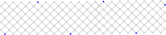
Figure 5: $VG^{1}_{4,20}$

Similarly, define $R_{2}=\{(2mt,m[1+(-1)^{t+1}])\quad;0\leq t\leq\lceil\frac{n-1}{m}\rceil-1\}$. The set $R_{2}\cup(x,y)$ is a resolving set for $VG^{2}_{m,n}$ with size $\lceil\frac{n-1}{m}\rceil+1$,
where,

$$(x,y)=\left\{\begin{array}[]{ll}(2n-2,2(n+m-\lceil\frac{n-1}{m}\rceil m-1);&\text{if}\enspace\lceil\frac{n-1}{m}\rceil\enspace\text{is odd},\\ (2n-2,2(\lceil\frac{n-1}{m}\rceil m-n+1));&\text{if}\enspace\lceil\frac{n-1}{m}\rceil\enspace\text{is even}.\\ \end{array}\right.$$

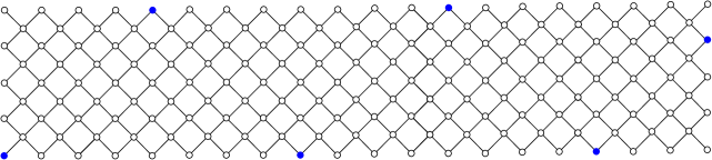
Figure 6: $VG^{2}_{4,20}$

4 Conclusion

The Villarceau grid is a geometric structure that emerges from the intersection of a cylinder and a plane, creating a unique pattern of circles on the surface of a torus. While it might seem like an abstract concept, its applications go beyond pure mathematics. This grid offers a hands-on way to explore and understand the complex shapes and properties of tori. In the world of computer graphics and visualization, the Villarceau grid can be used to create striking visual effects and simulate curved surfaces with precision. Its intricate design has the potential to inspire new ideas in architecture and design, where the principles behind the grid could lead to innovative structures and patterns. Furthermore, the grid is relevant in scientific fields where toroidal shapes play a crucial role, such as in the design of fusion reactors or the study of fluid dynamics. By providing a clearer understanding of these shapes, the Villarceau grid can contribute to advances in technology and engineering. In short, it is a tool that bridges the gap between abstract mathematics and real-world applications.
Data availability: No data associated with the manuscript.
Declarations:
Conflict of interest: The authors declare that there is no conflict of interest regarding the publication of this paper.

References

• [1] S. Khuller, B. Ragavachari, A. Rosenfield, Landmarks in graphs, Discrete Applied Mathematics 70(3) (1996) 217–229.
• [2] G. Chartrand, L. Eroh, M.A. Johnson, O. Oellermann, Resolvability in graphs and the metric dimension of a graph, Discrete Applied Mathematics 105(1) (2000) 99–113.
• [3] M.A. Johnson, Structure-activity maps for visualizing the graph variables arising in drug design, Journal of Biopharmaceutical Statistics 3 (1993) 203–236.
• [4] R.A. Melter, I. Tomescu, Metric bases in digital geometry, Computer Vision Graphics and Image Processing 25 (1984) 113–121.
• [5] A. Sebö, E. Tannier, On metric generators of graphs, Mathematics of Operations Research 29(2) (2004) 383–393.
• [6] K. Liu, N. Abu-Ghazaleh, Virtual coordinate backtracking for void traversal in geographic routing, Lecture Notes in Computer Science 4104 (2006) 46–59.
• [7] W. Goddard, Statistic mastermind revisited, Journal of Combinatorial Mathematics and Combinatorial Computing 51 (2004) 215–220.
• [8] Z. Beerliova, F. Eberhard, T. Erlebach, A. Hall, M. Hoffman, M. Mihalák, Network discovery and verification, IEEE Journal on Selected Areas in Communications 24(12) (2006) 2168–2181.
• [9] S. Söderberg, H.S. Shapiro, A combinatory detection problem, American Mathematical Monthly 70 (1963) 1066–1070.
• [10] J. Caceres, C. Hernando, M. Mora, I.M. Pelayo, M.L. Puertas, C. Seara, D.R. Wood, On the metric dimension of Cartesian products of graphs, SIAM Journal on Discrete Mathematics 21(2) (2007) 423–441.
• [11] F. Harary, R.A. Melter, On the metric dimension of a graph, Ars Combinatoria 2 (1976) 191–195.
• [12] S. Prabhu, S. Deepa, M. Arulperumjothi, L. Susilowati, J.B. Liu, Resolving-power domination number of probabilistic neural networks, Journal of Intelligent & Fuzzy Systems 43(5) (2022) 6253-6263.
• [13] M. Arulperumjothi, S. Klavžar, S. Prabhu, Redefining fractal cubic networks and determining their metric dimension and fault-tolerant metric dimension, Applied Mathematics and Computation 452 (2023) 128037.
• [14] S. Prabhu, D.S.R. Jeba, M. Arulperumjothi, S. Klavžar, Metric dimension of irregular convex triangular networks, AKCE International Journal of Graphs and Combinatorics (2023) DOI: 10.1080/09728600.2023.2280799.
• [15] S. Prabhu, V. Manimozhi, M. Arulperumjothi, S. Klavžar, Twin vertices in fault-tolerant metric sets and fault-tolerant metric dimension of multistage interconnection networks, Applied Mathematics and Computation 420 (2022) 126897.
• [16] S. Hayat, A. Khan, M.Y.H. Malik, M. Imran, M.K. Siddiqui, Fault-tolerant metric dimension of interconnection networks, IEEE Access 8 (2020) 145435–145445.
• [17] H. Raza, S. Hayat, M. Imran, X. Pan, Fault-Tolerant resolvability and external structures of graphs, Mathematics, 7(1) (2019) 78.
• [18] S. Prabhu, V. Manimozhi, A. Davoodi, J.L.G. Guirao, Fault-tolerant basis of generalized fat trees and perfect binary tree derived architectures, Journal of Supercomputing 80 (2024) 15783–15798.
• [19] P. Manuel, B. Rajan, I. Rajasingh, M.C. Monica, Landmarks in torus networks, Journal of Discrete Mathematical Sciences and Cryptography 9(2) (2006) 263–271.
• [20] A. Behtoei, A. Davoodi, M. Jannesari, B. Omoomi, A characterization of some graphs with metric dimension two, Discrete Mathematics, Algorithms and Applications 9(2) (2017) 1750027.
• [21] A. Kelenc, N. Tratni, I.G. Yero, Uniquely identifying the edges of a graph: The edge metric dimension, Discrete Applied Mathematics 251 (2018) 204–220.
• [22] P. Manuel, M.I. Abd-El-Barr, I. Rajasingh, B. Rajan, An efficient representation of Benes networks and its applications, Journal of Discrete Algorithms 6(1) (2008) 11–19.
• [23] A.F. Beardon, Resolving the hypercube, Discrete Applied Mathematics 161(13) (2013) 1882–1887.
• [24] B. Rajan, S.K. Thomas, M.C. Monica, Conditional resolvability of honeycomb and hexagonal networks, Mathematics in Computer Science 5(1) (2011) 89–99.
• [25] P. Manuel, B. Rajan, I. Rajasingh, M.C. Monica, On minimum metric dimension of honeycomb networks, Journal of Discrete Algorithms 6(1) (2008) 20–27.
• [26] B. Rajan, I. Rajasingh, P. Venugopal, M.C. Monica, Minimum metric dimension of illiac networks, Ars Combinatoria 117 (2014) 95–103.
• [27] B. Rajan, I. Rajasingh, M.C. Monica, P. Manuel, Metric dimension of enhanced hypercube networks, Journal of Combinatorial Mathematics and Combinatorial Computing 67 (2008) 5–15.
• [28] Z. Shao, S.M. Sheikholeslami, P. Wu, J. Liu, The metric dimension of some generalized Petersen graphs, Discrete Dynamics in Nature and Society 10 (2018) 4531958.
• [29] M. Imran, A.Q. Baig, S.A.U.H. Bokhary, I. Javaid, On the metric dimension of circulant graphs, Applied Mathematics Letters 25(3) (2012) 320–325.
• [30] T. Vetrík, The metric dimension of circulant graphs, Canadian Mathematical Bulletin 60(1) (2017) 206–216.
• [31] C. Grigorious, P. Manuel, M. Miller, B. Rajan, S. Stephen, On the metric dimension of circulant and Harary graphs, Applied Mathematics and Computation 248 (2014) 47–54.
• [32] J.B. Liu, M.F. Nadeem, M.A. Siddiqui, W. Nazir, Computing metric dimension of certain families of Toeplitz graphs, IEEE Access 7 (2019) 126734–126741.
• [33] J. Cáceres, C. Hernando, M. Mora, I.M. Pelayo, M.L. Puertas, On the metric dimension of infinite graphs, Electronic Notes in Discrete Mathematics 35 (2009) 15–20.
• [34] M. Fehr, S. Gosselin, O.R. Oellermann, The metric dimension of Cayley digraphs, Discrete Mathematics 306(1) (2006) 31–41.
• [35] R.F. Bailey, J. Cáceres, D. Garijo, A. González, A. Márquez, K. Meagher, M.L. Puertas, Resolving sets for Johnson and Kneser graphs, European Journal of Combinatorics 34(4) (2013) 736–751.
• [36] H. Fernau, P. Heggernes, P. Hof, D. Meister, R. Saei, Computing the metric dimension of chain graphs, Information Processing Letters 115(9) (2015) 671–676.
• [37] S. Akhter, R. Farooq, Metric dimension of fullerene graphs, Electronic Journal of Graph Theory and Applications 7(1) (2019) 91–103.
• [38] R.F. Bailey, K. Meagher, On the metric dimension of Grassmann graphs, Discrete Mathematics and Theoretical Computer Science 13(4) (2011) 97–104.
• [39] J. Kratica, V. Kovačević-Vujčić, M. Čangalović, M. Stojanović, Minimal doubly resolving sets and the strong metric dimension of some convex polytopes, Applied Mathematics and Computation 218(19) (2012) 9790–9801.
• [40] M. Imran, H.M.A. Siddiqui, Computing the metric dimension of convex polytopes generated by wheel related graphs, Acta Mathematica Hungarica 149(1) (2016) 10–30.
• [41] M. Hallaway, C.X. Kang, E. Yi, On metric dimension of permutation graphs, Journal of Combinatorial Optimization 28(4) (2014) 814–826.
• [42] M. Feng, K. Wang, On the metric dimension of bilinear forms graphs, Discrete Mathematics 312(6) (2012) 1266–1268.
• [43] J. Guo, K. Wang, F. Li, Metric dimension of symplectic dual polar graphs and symmetric bilinear forms graphs, Discrete Mathematics 313(2) (2013) 186–188.
• [44] H.M.A. Siddiqui, M. Imran, Computing the metric dimension of wheel related graphs, Applied Mathematics and Computation 242 (2014) 624–632.
• [45] R.F. Bailey, On the metric dimension of incidence graphs, Discrete Mathematics 341(6) (2018) 1613–1619.
• [46] J. Guo, K. Wang, F. Li, Metric dimension of some distance-regular graphs, Journal of Combinatorial Optimization 26 (2013) 190–197.
• [47] C. Poisson, P. Zhang, The metric dimension of unicyclic graphs, Journal of Combinatorial Mathematics and Combinatorial Computing 40 (2002) 17–32.
• [48] R.C. Tillquist, R.M. Frongillo, M.E. Lladser, Getting the lay of the land in discrete space: A survey of metric dimension and its applications, SIAM Review 65(4) (2023), 919–962.
• [49] S. Crevals, P.R.J. Östergård, Independent domination of grids, Discrete Mathematics 338 (2015) 1379–1384.
• [50] L. Saha, M. Basak, K. Tiwary, All metric bases and fault-tolerant metric dimension for square of grid, Opuscula Mathematica 42(1) (2022) 93–111.
• [51] B.D. Acharya, M.K. Gill, On the index of gracefulness of a graph and the gracefulness of two dimensional square lattice graphs, Indian Journal of Mathematics 23 (1981) 81–94.
• [52] C.C. Lee, J. M. Hervé, Oblique circular torus, Villarceau circles, and four types of Bennett linkages, Journal of Mechanical Engineering Science, 228(4) (2014) 742–752.
• [53] P. Manuel, Properties of Villarceau torus, arXiv:2306.09632 (2023).