radarODE-MTL: A Multi-Task Learning Framework with Eccentric Gradient Alignment for Robust Radar-Based ECG Reconstruction

Abstract

Millimeter-wave radar is promising to provide robust and accurate vital sign monitoring in an unobtrusive manner. However, the radar signal might be distorted in propagation by ambient noise or random body movement, ruining the subtle cardiac activities and destroying the vital sign recovery. In particular, the recovery of electrocardiogram (ECG) signal heavily relies on the deep-learning model and is sensitive to noise. Therefore, this work creatively deconstructs the radar-based ECG recovery into three individual tasks and proposes a multi-task learning (MTL) framework, radarODE-MTL, to increase the robustness against consistent and abrupt noises. In addition, to alleviate the potential conflicts in optimizing individual tasks, a novel multi-task optimization strategy, eccentric gradient alignment (EGA), is proposed to dynamically trim the task-specific gradients based on task difficulties in orthogonal space. The proposed radarODE-MTL with EGA is evaluated on the public dataset with prominent improvements in accuracy, and the performance remains consistent under noises. The experimental results indicate that radarODE-MTL could reconstruct accurate ECG signals robustly from radar signals and imply the application prospect in real-life situations. The code is available at: http://github.com/ZYY0844/radarODE-MTL.

I Introduction

Electrocardiogram (ECG) signal is commonly recognized as the golden standard in cardiac monitoring compared with other vital signs (e.g., heart rate, photoplethysmography), because ECG describes the fine-grained cardiac activities, such as atrial/ventricular depolarization/repolarization, through the featured waveform (i.e., PQRST peaks) and is crucial to the diagnosis of cardiovascular diseases [1]. The traditional ECG measurement relies on the adhesive electrode patches with wired connections to the monitor to provide real-time and accurate ECG signals and is mainly used in clinical scenarios due to the cumbersome apparatus. However, the contact-based ECG collection is unfriendly to long-term monitoring and is not applicable to daily wellness monitoring [2]. Recently, radar has become a promising contactless sensor to provide non-invasive and accurate ECG monitoring by using advanced signal-processing algorithm and deep neural network [2, 3, 4, 5].

The trials on the radar-based ECG recovery can be categorized into two paradigms. The first paradigm only performs the extraction of high-resolution cardiac mechanical activities to produce quasi-ECG signals, omitting the morphological ECG features while maintaining certain fine-grained features. For example, the mostly adopted quasi-ECG signal only preserves R and T peaks and can be realized by signal decomposition [6] or state estimation [7, 8]. In contrast, the second paradigm aims to reconstruct the ECG waveform as measured by clinical apparatus, because the doctor and ECG analysis toolbox all rely on the shape of ECG to make diagnosis [9]. However, decoupling the ECG signal from the measured radar signal requires establishing an extremely complex model from the perspective of electrophysiology (i.e., excitation-contraction coupling [1]), and the existing research can only leverage deep learning methods to learning such domain transformation from the dataset containing numerous radar/ECG pairs [2, 3, 4, 5].

In the literature, radar-based ECG waveform recovery has been achieved based on various deep-learning architectures, such as convolutional neural network (CNN) [2, 5], long short-term memory (LSTM) network [7], and Transformer [2, 3]. However, the noise robustness of the deep-learning framework is rarely investigated in the literature, especially for the random body movement (RBM) noise that is inevitable in contactless monitoring and has orders of magnitude larger than cardiac activities. The existing work either discarded the data during the RBM [4] or reported the heavy distortion as the future work [2]. Additionally, the existing deep-learning methods are also blamed for being purely data-drove as a black box and the transformation between cardiac mechanical and electrical activities lacks the theoretical explanation [5].

Based on the limitations of the existing methods, it is necessary to provide a feasible model that explains the transformation inside radar-based long-term ECG recovery and is also robust to real-life noises. Therefore, this work proposes to deconstruct the radar-based ECG reconstruction into three individual tasks as a multi-task learning (MTL) problem to extract cardiac features with different levels of granularity, i.e., coarse features: heartbeat detection and cardiac cycle timing; fine-grained feature: ECG waveform. However, another consequent problem is to simultaneously optimize three individual tasks under the MTL paradigm, because the optimization of one task may degrade the performance of the others [10, 11].

In the literature, MTL is a widely-used deep learning paradigm in various fields such as scene understanding [12, 13], autonomous driving [14] and speech/text processing [15]. However, the MTL paradigm has never been applied in radar-based ECG recovery, and the existing MTL optimization strategies cannot fairly optimize all the tasks due to the imbalanced task difficulties [16]. In this work, the difficulty of extracting the ECG waveform is much higher than the other two, and simply applying the existing optimization strategies cannot achieve an ideal result with fair improvements on all tasks according to our initial experiments.

Inspired by the above discussion, the contributions of this work can be concluded as:

• A novel optimization strategy called eccentric gradient alignment (EGA) is proposed for updating shared parameters in the MTL neural network, aiming to balance the intrinsic difficulty across tasks during network training and also prevent the negative transfer phenomenon.

• To the best of our knowledge, this is the first work that models the radar-based long-term ECG recovery as three tasks and realized by an end-to-end MTL framework named radarODE-MTL, improving the robustness against both constant and abrupt noises.

• Sufficient experiments show that the proposed radarODE-MTL with EGA optimization strategy outperforms other frameworks and optimization strategies under various noise conditions and datasets.

The rest of the paper is organized as follows. Section II provides the background for radar-based ECG recovery and MTL optimization. The proposed radarODE-MTL framework with EGA strategy is elaborated in Section III, and the experimental settings and results are shown in Section IV. At last, Section V concludes this paper with future work.

II Background and Problem Statement

This section will provide compact explanations of the domain transformation in ECG recovery and the optimization problem in MTL network, with the corresponding problem statements.

II-A Model for Domain Transformation and Problem Statement

II-A1 Signal Model for Cardiac Mechanical Activities

The first step for any contactless vital sign monitoring is to obtain the displacement near the chest region by unwrapping the chest displacement $\tilde{x}(t)$ from the phase change $\Delta\phi(t)$ of the received radar signal with wavelength $\lambda$ as:

$$\Delta\phi(t)=\frac{4\pi\tilde{x}(t)}{\lambda}$$ (1)

The demodulated chest displacement contains the interested cardiac mechanical activities with multiple noises, such as respiration noise [17] and RBM noise [2]. In ECG recovery, some periodic or high-frequency noise can be filtered in pre-processing following the methods in [6], while some constant or abrupt noises are hard to remove. Therefore, the original chest displacement $\tilde{x}(t)$ can be processed to $x(t)$ for ECG recovery after initial noise removal as:

$$x(t)=x_{c}(t)+n_{abr}(t)+n_{con}(t)$$ (2)

where $x_{c}(t)$ contains the interested cardiac mechanical activities, $n_{abr}(t)$ represents the abrupt noises (e.g., RBM) and $n_{con}(t)$ describes many other constant noises that affect the signal-to-noise ratio (SNR), such as thermal noise [6, 18], monitoring from random directions [19] and long-range monitoring [17].

According to our previous work [5], the fine-grained cardiac mechanical activities include aortic valve opening/closure (AO/AC) and mitral valve opening/closure (MO/MC), revealed by the corresponding prominent vibrations $v_{1}$ and $v_{2}$ as measured in radar signal $x(t)$ as depicted in Figure 1. Therefore, the signal model $x(t)$ can be further refined into subtle cardiac activities for $K$ cardiac cycles as:

$$x(t)=\sum_{k=1}^{K}v^{k}_{1}(t)+\sum_{k=1}^{K}v^{k}_{2}(t)+n_{abr}(t)+n_{con}(t)$$ (3)

with

$$v^{k}_{1}(t) =\mathrm{a}^{k}_{1}\mathrm{cos}(2\pi f^{k}_{1}t)\exp\left(-\frac{(t-T^{k}_{1})^{2}}{{b^{k}_{1}}^{2}}\right)$$ (4)

$$v^{k}_{2}(t) =\mathrm{a}^{k}_{2}\mathrm{cos}(2\pi f^{k}_{2}t)\exp\left(-\frac{(t-T^{k}_{2})^{2}}{{b^{k}_{1}}^{2}}\right)$$

where $a_{1}^{k}$, $b_{1}^{k}$ and $a_{2}^{k}$, $b_{2}^{k}$ jointly determine the amplitudes and lengths of the first and second prominent vibrations for $k^{th}$ cardiac cycle, $f_{1}^{k}$, $f_{2}^{k}$ are the corresponding central frequencies and $T_{1}^{k}$, $T_{2}^{k}$ represent when the vibrations happen.

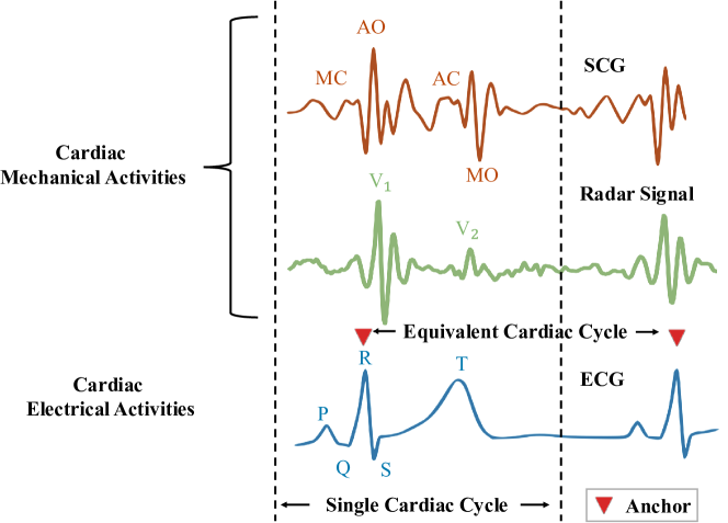
Figure 1: Relationships between cardiac mechanical and electrical activities, with single cardiac cycle and ECG anchors labeled.

II-A2 Model of Domain Transformation

The radar signal modeled in (3) shares a strong temporal consistency with the ECG signal as shown in Figure 1, because the excitation-contraction coupling indicates that the electrical signal (ECG) triggers the heart muscle contraction (SCG) [1]. Therefore, this work proposed to deconstruct the radar-based ECG recovery into three tasks to realize the robust transformation from the measured radar signal $x(t)$ to the ECG signal, and the three tasks can be modeled as:

• Task $1$: The reconstruction of the morphological features aims to learn the mapping function $\mathcal{T}(\cdot)$ only for the single-cycle cardiac activities from $x(t)$ to the ECG pieces as $x_{ecg}(t)=\mathcal{T}(x(t))$.

• Task $2$: The detection of R peaks (anchors) is equivalent to finding $\mathbf{R}=\{T^{1}_{1},T^{2}_{1},\cdots,T^{K}_{1}\}$ in (4) according to the central frequency $f^{k}_{1}$ of $v^{k}_{1}$, as shown in Figure 1.

• Task $3$: The prediction of the length of a single cardiac cycle is equivalent to finding the distance between successive anchors (i.e., peak-to-peak interval (PPI)) as $PPI^{k}=T_{1}^{k+1}-T_{1}^{k}$, as shown in Figure 1.

II-A3 Problem Statement for Domain Transformation

The main problem in the existing domain transformation methods can be summarized as follows:

• The transformation between arbitrary radar/ECG pairs is hard to model, and hence the ECG recovery process is vulnerable to the noises with bad root mean square error (RMSE) and Pearson correlation coefficient (PCC) as shown in Figure LABEL:sub@fig:distorted_ecg.

• Although the model for the domain transformation between single-cycle radar/ECG pair has been proposed in [5], the long-term ECG recovery might be misaligned with ground truth due to inaccurate PPI estimation [5], deteriorating the RMSE/PCC even if the morphological features are well-recovered as shown in Figure LABEL:sub@fig:mis_ecg.

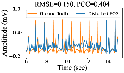
(a)

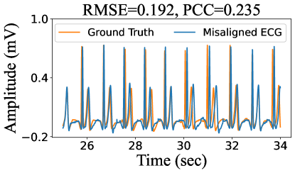
(b)

Figure 2: The impact of strong noise and misalignment: (a) ECG recovery distorted by RBM noise [2]; (b) Misaligned ECG recovery due to the inaccurate PPI estimation [5].

In addition, the constant and abrupt noises heavily affect the quality of contactless cardiac monitoring and have been investigated a lot, especially for the algorithms in coarse cardiac feature monitoring [6, 17, 19]. However, the fine-grained ECG recovery could only realized by deep-learning methods, and the noise robustness of the deep-learning model has never been evaluated in the literature [2, 4, 3, 5]. Therefore, radarODE-MTL dissects the long-term ECG recovery into three tasks, and hence each decoder only focuses on extracting the cardiac feature with different granularity, aiming to improve the accuracy and noise robustness of the radar-based ECG recovery.

II-B Optimization Strategies for MTL

II-B1 Optimization of MTL Network

A standard definition for an MTL optimization problem with $n$ tasks under hard parameter sharing (HPS [20]) architecture is given by:

$$\boldsymbol{\theta}^{*}=\underset{\boldsymbol{\theta}\in\mathbb{R}^{m}}{\arg\min}\left\{\mathcal{F}(\boldsymbol{\theta})\triangleq\frac{1}{n}\sum_{i=1}^{n}\mathcal{L}_{i}(\boldsymbol{\theta})\right\}$$ (5)

where $\boldsymbol{\theta}\in\mathbb{R}^{m}$ denotes the shared parameter space, $\mathcal{L}_{i}(\boldsymbol{\theta})$ is the task-specific non-negative objective function for $\mathbb{R}^{m}\rightarrow\mathbb{R}_{+}$, and $\mathcal{F}(\boldsymbol{\theta})$ represents a mapping from the parameter space to the objective space as $\mathbb{R}^{m}\rightarrow\mathbb{R}^{n}$. The MTL optimization strategy aims to find the optimal parameter set $\boldsymbol{\theta}^{*}$ that minimizes the average loss.

The dilemma in the design of MTL optimization strategies is mainly on avoiding negative transfer when the optimization of individual tasks conflicts with each other [21, 22, 23, 24, 25, 26, 27, 28], spawning two main categories of methods, loss balancing method and gradient balancing methods, to impartially search for the optimal solution(s) subjecting to Pareto optimality [24].

The loss balancing methods add the weight to each task loss $\mathcal{L}_{i}(\boldsymbol{\theta})$ based on various criteria, such as learning rate [26], inherent task uncertainty [28] or the loss magnitude [23]. In contrast, gradient balancing methods address the negative transfer by balancing both magnitudes and the directions of the task-specific gradient $\boldsymbol{g}_{i}=\nabla_{\boldsymbol{\theta}}\mathcal{L}_{i}(\boldsymbol{\theta})$, according to certain criteria such as the cosine similarity between gradients [24], descending rate [24] or the orthogonality of the gradient system [21].

II-B2 Problem Statement for Designing MTL Optimization Strategies

The existing methods perform not well on the proposed radarODE-MTL framework because most methods aim to treat all the tasks equally and pay too much attention to the easy tasks with the least achievement after convergence (e.g., slow learning rate in GradNorm [29], small singular value in Aligned-MTL [21]), while the hard task tolerates a slow convergence rate due to the limited gradient magnitudes or update frequencies [16]. Several studies in the literature proposed to increase the weight for the hard task metered the learning rate [16, 30]. However, the forcible change of the weight may aggravate the gradient conflict and hence degrade other tasks, because the loss-balancing method can not alleviate the gradient conflict issue [24].

In addition, the slow learning rate can be interpreted in two ways: (a) The optimization stalls due to the compromise in gradients normalization, and the constraint on the hard task should be released as adopted in GradNorm [29] and DWA [26]; (b) The optimization has already achieved convergence and should be terminated as in the early stop technique [31]. Unfortunately, it is hardly investigated whether the optimization actually converges or stalls, or say, should more computational resources be skewed towards the task with limited learning progress. Therefore, EGA is proposed in this paper to estimate the intrinsic task difficulty based on the current learning progress and dynamically alter the gradients in orthogonal space to fairly benefit all the tasks without knowing the actual optimization status (i.e., stall or convergence).

III Methodology

III-A Overview of radarODE-MTL with EGA Strategy

The aforementioned three deconstructed tasks for radar-based ECG recovery can be realized by the proposed radarODE-MTL framework as shown in Figure 3, and the dataset used for training and validation is provided in [2]. Firstly, the $50$ synchronous radar signals will be pre-processed into spectrograms by synchrosqueezed wavelet transform (SST) to highlight the central frequencies for locating the prominent vibrations $v_{1}$ and $v_{2}$. Then, radarODE-MTL is designed to generate the long-term ECG recovery in an end-to-end manner with certain shared layers to capture the common representations for all tasks and three task-specific decoders to recover the ECG morphological features, detect ECG anchors (R peaks) and estimate single-cardiac-cycle length respectively, as shown in Figure 3(a)-(d).

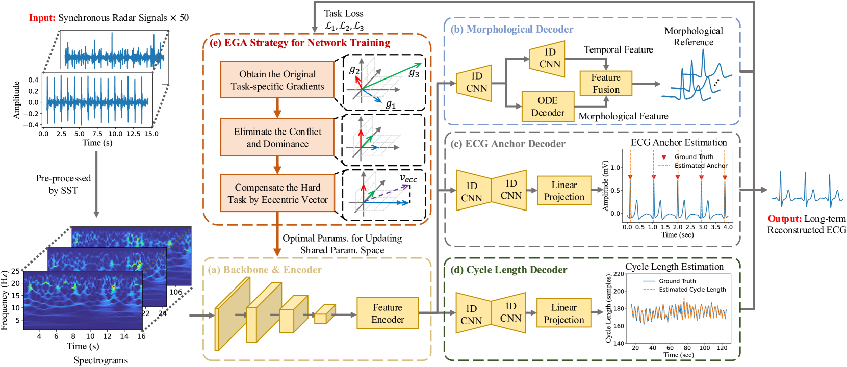
Figure 3: Overview of the radarODE-MTL framework with EGA strategy: (a) Shared backbone extracts time-frequency features from the signal spectrograms; (b) Morphological decoder only reconstructs the shape of the current ECG piece; (c) ECG anchor decoder estimates the time-index of anchors (R peaks); (d) Cycle length decoder estimates the length of the current cardiac cycle; (e) The proposed EGA strategy for optimizing shared parameter space.

During the training stage, the network optimization of three decoders follows the standard single-task optimization method, and the share parameter space (Backbone$\&$Encoder) is updated using the proposed EGA strategy based on the task-specific loss $\mathcal{L}_{1},\mathcal{L}_{2},\mathcal{L}_{3}$, as shown in Figure 3(e). In general, the EGA strategy first tries to eliminate the conflict and dominance among the original task-specific gradients, e.g., $\boldsymbol{g_{1}}$, $\boldsymbol{g_{2}}$ have opposite directions and $\boldsymbol{g_{3}}$ has large magnitude. Secondly, the eccentric vector ($v_{ecc}$) is introduced for balancing the task difficulties to fairly optimize all the tasks.

Remark 1

The latent information needed in different tasks can be broadcasted across layers to improve the generalization of the model and the performance of every single task [10, 21]. Therefore, in addition to the design of optimization strategies, challenges also arise to designing the efficient MTL structure for knowledge sharing that benefits all the tasks [26].

III-B Backbone and Encoder

The backbone of radarODE-MTL is used to extract the latent features from the input SST spectrograms and is expected to figure out the remarkable patterns for vibrations $v_{1}$ and $v_{2}$ with certain central frequencies and periodicity. Specifically, ResNet is adopted in this work as the backbone and has been proven to be an efficient structure in computer vision or signal processing [32, 33, 34]. Then, the encoder contains only one 2D convolutional layer to further compress the feature in the time-frequency domain into the 1D time domain for later processing. The performance has been verified in our previous work with the detailed structure shown in [5].

III-C Morphological Decoder

The morphological decoder has been designed in our previous work radarODE [5] as the single cycle ECG generate (SCEG) module to realize the robust domain transformation in a single cardiac cycle with a fast rate of convergence, because an ODE model is introduced in the ODE decoder to provide morphological feature as the prior knowledge to guide/constrain the ECG recovery. Similarly, in radarODE-MTL, a morphological decoder will be used to realize the mapping function $\mathcal{T}(\cdot)$ in Task $1$ and generate morphological reference by fusing both temporal and morphological features, as shown in Figure 3(b).

III-D ECG Anchor Decoder and Cycle Length Decoder

The ECG anchor decoder and cycle length decoder are designed to identify the time-domain anchors $T_{1}^{k}$ and single-cardiac-cycle length $PPI^{k}$ in Task $2$ and $3$ simultaneously for the accurate alignment of ECG pieces as shown in Figure 3(c) and (d), avoiding the impact of error accumulation in long-term ECG recovery [5]. In addition, the prediction of the ECG anchors and cycle lengths can leverage the context information even if the current cardiac cycle is ruined by noises, because the vital signs are nearly unchanged for healthy people in successive cardiac cycles [8].

The structures of the ECG anchor decoder and cycle length decoder are the same as shown in Figure 3(c) and (d), with several layers of 1D CNN-based encoder/decoder followed by a linear projection block. Specifically, the encoder is assembled by four 1D CNN blocks with each block containing 1D convolution, batch normalization (BN) and rectified linear unit (ReLU) activation function; the decoder is composed of two 1D transposed CNN blocks with each block containing 1D transposed convolution, BN and ReLu; and the linear projection block is assembled by linear layer, BN and ReLU with one linear layer appended at last as the output layer.

III-E Input, Output and Loss Function

The inputs of radarODE-MTL are the $4$-sec segments divided from long-term radar signal with a step length of $1$ sec, and the middle cardiac cycle is selected as the ground truth ECG piece. Then, to calculate the loss value, the ground truth ECG piece should be resampled as a fixed length $200$ to match the output dimension, and the RMSE is used to calculate $\mathcal{L}_{1}$. The output of the ECG anchor decoder should contain multiple predicted anchors within $4$-sec segment, and the cross-entropy loss is used for $\mathcal{L}_{2}$ calculation as a multi-class classification problem (i.e., each time index acts as a possible class). Differently, the output of the cycle length decoder only represents the length of the current evaluated cardiac cycle with only one true label (value = $1$), and the cross-entropy loss is used for $\mathcal{L}_{3}$ calculation as a one-class classification problem.

Eventually, the calculated $\mathcal{L}_{1},\mathcal{L}_{2},\mathcal{L}_{3}$ will be used for optimization using the later proposed EGA strategy during training, otherwise the three outputs can directly form the long-term ECG recovery by aligning the recovered ECG pieces (Task $1$) with the predicted anchors (Task $2$) after resampling the ECG pieces as the cycle lengths (Task $3$).

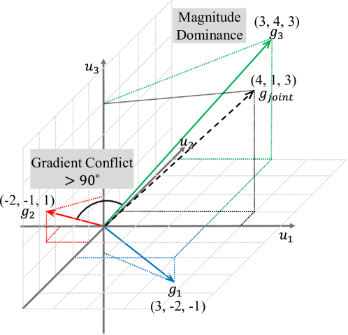
(a)

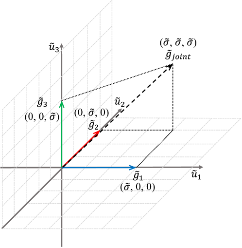
(b)

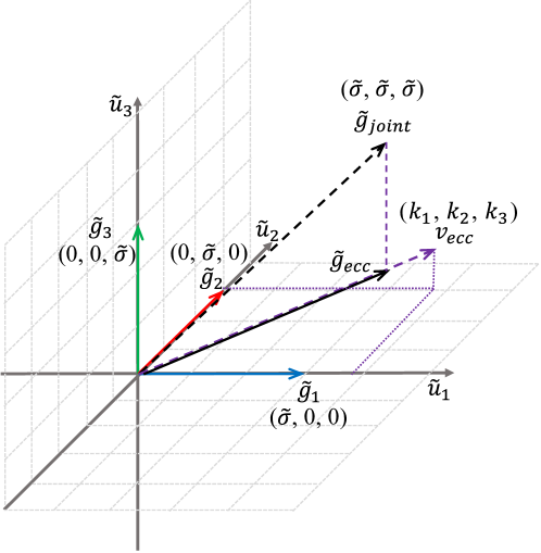
(c)

Figure 4: Illustration of EGA: (a) Original gradient space with gradient conflict and magnitude dominance; (b) The projection of the original gradient space into the orthogonal space with equal “learning rate”; (c) The implementation of eccentric gradient alignment to skew the joint gradient $\tilde{g}_{joint}$ towards the hard task by introducing the eccentric vector $v_{ecc}$.

III-F Eccentric Gradient Alignment (EGA) Strategy

According to the discussion in Section II-B, the imbalanced difficulties among three tasks will raise a new challenge to not only simultaneously optimize all the tasks without negative transfer [25], but also keep improving the hard tasks even if the easy tasks have already achieved convergence.

In this case, EGA first needs to solve the gradient conflict and magnitude dominance within the original task-specific gradients $\boldsymbol{g}_{1}$, $\boldsymbol{g}_{2}$, $\boldsymbol{g}_{3}$ as shown in Figure LABEL:sub@fig:grad_conflict, e.g., $\boldsymbol{g}_{1}$ and $\boldsymbol{g}_{2}$ may have opposite directions hence canceling with each other, and $\boldsymbol{g}_{3}$ may have a large magnitude hence dominating the linear combination of all the gradients, with the resultant $\boldsymbol{g}_{joint}$ leaning on $\boldsymbol{g}_{3}$. A common solution is to project all the gradients into an orthogonal space to eliminate gradient conflict [21, 35], and hence the optimization based on $\boldsymbol{g}_{joint}$ will not degrade any of the tasks. Then, the magnitude of the gradients will be unified as the same value (e.g., $\tilde{\sigma}$) to obtain new task-specific gradients $\tilde{\boldsymbol{g}}_{1}$, $\tilde{\boldsymbol{g}}_{2}$, $\tilde{\boldsymbol{g}}_{3}$, as shown in Figure LABEL:sub@fig:grad_orth.

Furthermore, instead of categorically selecting the hard task based on the learning rate and only increasing the corresponding weight, EGA creatively provides an adjustable estimation of the intrinsic task difficulty by mapping the learning rate through a softmax with hyperparameter $T$. In other words, suitable intrinsic task difficulty can be obtained by adjusting $T$ without knowing the actual optimization status (i.e., stall or convergence), and the discrepancy among task difficulties can be adjusted to avoid overlooking or overrating any task. In practice, to integrate the estimated intrinsic task difficulty with MTL optimization, EGA proposed to add an eccentric vector $\boldsymbol{v}_{ecc}$ to eccentrically align the joint gradient $\tilde{\boldsymbol{g}}_{joint}$ to the hard task, as shown in Figure LABEL:sub@fig:grad_ecc.

The detailed EGA strategy will be explained in this section in terms of the preparation stage, gradient projection and normalization, and eccentric gradient alignment.

III-F1 Preparations for EGA Optimization

As a gradient-based MTL optimization method with objective function in (5), EGA requires to access task-specific gradient in terms of the shared parameters $\boldsymbol{\theta}$, and the gradients can be obtained as $\boldsymbol{g}_{i}=\nabla_{\boldsymbol{\theta}}\mathcal{L}_{i}(\boldsymbol{\theta}),i\in[n]$, forming the original gradient matrix as $\boldsymbol{G}=\{\boldsymbol{g}_{1},\cdots,\boldsymbol{g}_{i}\}\in\mathbb{R}^{n\times m}$. Then, the joint gradient for optimizing the shared parameter space can be linearly combined as $\boldsymbol{g}_{joint}=\boldsymbol{G^{\intercal}w}$, with $\boldsymbol{w}=[1,\cdots,1]^{\intercal}$ representing the weights for each $\boldsymbol{g}_{i}$. The original gradient matrix $\boldsymbol{G}$ normally has gradient conflict and magnitude dominance issues, as shown in Figure LABEL:sub@fig:grad_conflict.

III-F2 Gradients Projection and Normalization

In order to solve the conflict inside the gradient matrix $\boldsymbol{G}$, the orthogonal projection problem can be formulated as finding a gradient matrix $\boldsymbol{\tilde{G}}$ with the new joint gradient $\boldsymbol{\tilde{g}}_{joint}=\boldsymbol{\tilde{G}^{\intercal}w}$ close to the original $\boldsymbol{g}_{joint}$:

$$\min\|\boldsymbol{g}_{joint}-\boldsymbol{\tilde{g}}_{joint}\|_{2}^{2}\quad\text{ s.t. }\ \tilde{\boldsymbol{G}}\tilde{\boldsymbol{G}}^{\intercal}=\boldsymbol{I}$$ (6)

Then, according to the derivation based on triangle inequality:

$$\left\|\boldsymbol{g}_{joint}-\tilde{\boldsymbol{g}}_{joint}\right\|_{2}^{2}=\left\|\boldsymbol{G^{\intercal}w}-{\boldsymbol{\tilde{G}^{\intercal}w}}\right\|_{2}^{2}\leq\|\boldsymbol{G^{\intercal}}-{\boldsymbol{\tilde{G}^{\intercal}}}\|_{F}^{2}\|\boldsymbol{w}\|_{2}^{2}$$ (7)

At last, the projection problem can be finally formulated as:

$$\min_{\tilde{\boldsymbol{G}}}\|\boldsymbol{G}-\tilde{\boldsymbol{G}}\|_{F}^{2}\quad\text{ s.t. }\ \tilde{\boldsymbol{G}}\tilde{\boldsymbol{G}}^{\intercal}=\boldsymbol{I}$$ (8)

The solution to the problem in (8) has been given in the orthogonal Procrustes problem [36] by simply applying singular value decomposition (SVD) to $\boldsymbol{G}$ as:

$$\boldsymbol{G}=\boldsymbol{U}\boldsymbol{\Sigma}\boldsymbol{V}^{\intercal}$$ (9)

Then, the orthogonal gradient matrix $\boldsymbol{\tilde{G}}$ with unit singular values can be obtained as:

$$\tilde{\boldsymbol{G}}=\boldsymbol{UV^{\intercal}}$$ (10)

In addition, the calculation can be simplified by applying the eigenvalue decomposition to the Gram matrices $\boldsymbol{GG^{\intercal}}$ as:

$$\boldsymbol{GG^{\intercal}}=\boldsymbol{U\left(\Sigma\Sigma^{\intercal}\right)U^{\intercal}}$$ (11)

Then, the final solution in (10) can be rewritten by combining (9) and (11) as:

$$\tilde{\boldsymbol{G}}=\boldsymbol{U\Sigma^{-1}U^{\intercal}G}$$ (12)

The current $\tilde{\boldsymbol{G}}$ in (12) is orthogonal but with unit singular values, and the next step is to re-scale the task-specific gradients to avoid magnitude dominance. According to the literature [21], the original magnitude of task-specific gradients is proportional to the singular values of $\tilde{\boldsymbol{G}}$. Therefore, to ensure the convergence to the optima of all the tasks, the minimal singular value is selected to calculate the scaling factor instead of using the original singular values, and the re-scaled $\tilde{\boldsymbol{G}}$ can be obtained as:

$$\tilde{\boldsymbol{G}}=\tilde{\sigma}\boldsymbol{U\Sigma^{-1}U^{\intercal}G},\quad\text{with}\ \tilde{\sigma}=\min(\sqrt{\text{eigenvalue}(\boldsymbol{GG^{\intercal}})})$$ (13)

At last, the orthogonal gradient matrix with equal magnitude is shown in Figure LABEL:sub@fig:grad_orth, but all the tasks are currently compromised on the same learning rate, causing the stall of the optimization for certain hard tasks.

Algorithm 1 EGA Optimization Strategy for MTL

1:Input:

Loss values for $n$ tasks $[\mathcal{L}_{1},\cdots,\mathcal{L}_{i}],i\in[n]$,

Shared parameters $\boldsymbol{\theta}$ and Step length $\eta$,

$T$ for softmax and $t_{warm}$ for warmup epoch

2:Output: Optimal parameters $\boldsymbol{\theta}^{*}$ for updating $\boldsymbol{\theta}$

3:Objective:

4:- Find the optimal parameter set $\boldsymbol{\theta}^{*}$ such that

5:$\boldsymbol{\theta}^{*}=\underset{\boldsymbol{\theta}\in\mathbb{R}^{m}}{\arg\min}\left\{\mathcal{F}(\boldsymbol{\theta})\triangleq\frac{1}{n}\sum_{i=1}^{n}\mathcal{L}_{i}(\boldsymbol{\theta})\right\}$

6:For the input batch in certain epoch:

7:- Initialize eccentric vector $\boldsymbol{v}_{ecc}=[1,\cdots,1]^{\intercal}\in\mathbb{R}^{n}$

8:- Get the current epoch as $t$

9:- Calculate task-specific gradient $\boldsymbol{g}_{i}=\nabla_{\boldsymbol{\theta}}\mathcal{L}_{i}(\boldsymbol{\theta}),i\in[n]$

10:- Form gradient matrix $\boldsymbol{G}=\{\boldsymbol{g}_{1},\cdots,\boldsymbol{g}_{i}\}\in\mathbb{R}^{n\times m}$

11:-

Calculate eigenvalues/eigenvectors of Gram matrix as in (11):

$\boldsymbol{GG^{\intercal}}=\boldsymbol{U\left(\Sigma\Sigma^{\intercal}\right)U^{\intercal}}$ with eigenvalues $\boldsymbol{\lambda}$

12:-

Get scaling factor: $\tilde{\sigma}=\min(\boldsymbol{\sqrt{\lambda}})$

13:-

Calculate the orthogonal and normalized gradient matrix as in (13): $\tilde{\boldsymbol{G}}=\tilde{\sigma}\boldsymbol{U\Sigma^{-1}U^{\intercal}G}$

14:if $t=t_{warm}$ then

15:     - Record the loss values for all the tasks $\mathcal{L}_{i}(t_{warm})$

16:else if $t>t_{warm}$ then

17:     -

Calculate the intrinsic task difficulty as in (15):

$k_{i}(t)=\text{softmax}(lr_{i}(t-1))$

18:     - Form eccentric vector $\boldsymbol{v}_{ecc}=[k_{1},\cdots,k_{i}]^{\intercal}$

19:end if

20:- Calculate final joint gradient $\boldsymbol{\tilde{g}}_{ecc}=\tilde{\boldsymbol{G}}^{\intercal}\boldsymbol{\boldsymbol{v}}_{ecc}$

21:- Calculate optimal parameters $\boldsymbol{\theta}^{*}=\boldsymbol{\theta}-\eta\boldsymbol{\tilde{g}}_{ecc}$

III-F3 Eccentric Gradient Alignment

To estimate the intrinsic task difficulty, the first step is to assess the current learning rate $lr_{i}$ based on the loss value $\mathcal{L}_{i}$ of each task:

$$lr_{i}(t-1)=\frac{\mathcal{L}_{i}(t-1)}{\mathcal{L}_{i}(t_{warm})}$$ (14)

with $\mathcal{L}_{i}(t-1)$ and $\mathcal{L}_{i}(t_{warm})$ representing the loss value for Task $i$ at the previous epoch and the warmup epoch (e.g., $t_{warm}=4$ in this paper), and the $lr_{i}$ is inversely proportional to the learning rate (i.e., small $lr_{i}$ for fast learning rate). Then, a softmax function is applied to mapping the $lr_{i}$ to the intrinsic task difficulty $k_{i}$ as:

$$k_{i}(t)=\text{softmax}(lr_{i}(t-1))=\frac{n\exp\left(lr_{i}(t-1)/T\right)}{\sum_{j=1}^{n}\exp\left(lr_{j}(t-1)/T\right)}$$ (15)

with $T$ controlling the discrepancy of the mapped task difficulties (i.e., small $T$ enlarges the discrepancy between $k_{i}$), and the summation of the weights should be $\sum_{i=1}^{n}k_{i}=n$. In addition, the intrinsic task difficult $k_{i}$ is positive without the negative transfer issue and can be formed as eccentric vector $\boldsymbol{v}_{ecc}=[k_{1},\cdots,k_{i}]^{\intercal}$ as in Figure LABEL:sub@fig:grad_ecc to guide the final joint gradient $\boldsymbol{\tilde{g}}_{ecc}$ for optimization as $\boldsymbol{\tilde{g}}_{ecc}=\tilde{\boldsymbol{G}}^{\intercal}\boldsymbol{\boldsymbol{v}}_{ecc}$. At last, the optimal parameter set $\boldsymbol{\theta}^{*}$ for updating the shared parameter space can be obtained after providing a step length $\eta$ based on the current parameter set $\boldsymbol{\theta}$ as $\boldsymbol{\theta}^{*}=\boldsymbol{\theta}-\eta\boldsymbol{\tilde{g}}_{ecc}$.

The entire EGA optimization strategy is summarized in Algorithm 1 to repeatedly update the shared parameter space (i.e., Backbone$\&$Encoder in this work) based on all the batches in each epoch, and the optimization will be terminated until achieving a pre-defined epoch number.

TABLE I: Comparison of different optimization strategies on radar-based ECG recovery

	ECG Shape Recovery		Cycle Length Estimation	ECG Anchor Estimation		$\Delta m\%\uparrow$
	RMSE (mV) $\downarrow$	PCC $\uparrow$	PPI Error (ms) $\downarrow$	Timing Error (ms) $\downarrow$	MDR $\downarrow$
Single-task baseline	0.106	86.6%	9.6	7.5	6.67%	0%
Loss Balancing Methods
Equal Weight	0.125	79.7%	8.0	9.7	5.51%	-0.73%
UW [28]	0.066	88.5%	11.2	5.5	6.44%	5.95%
GLS [27]	0.087	87.3%	14.1	6.7	4.32%	-4.65%
DWA [26]	0.133	80.7%	8.3	6.4	5.33%	4.84%
STCH [25]	0.070	88.0%	13.9	5.5	3.28%	3.90%
Gradient Balancing Methods
CAGrad [24]	0.107	84.2%	10.2	6.2	3.98%	6.72%
IMTL [23]	0.088	89.4%	9.3	6.0	6.22%	8.90%
MoCo [22]	0.179	61.0%	8.7	6.8	4.27%	-5.72%
Aligned-MTL [21]	0.092	87.9%	10.0	6.9	3.52%	10.26%
EGA ($T=0.1$)	0.119	79.0%	10.6	6.8	3.34%	2.74%
EGA ($T=0.5$)	0.082	89.6%	9.9	6.3	4.19%	12.10%
EGA ($T=1.0$)	0.085	87.4%	8.5	7.2	4.31%	13.95%
EGA ($T=1.5$)	0.105	82.9%	8.1	6.3	5.13%	10.95%
EGA ($T=2.0$)	0.091	86.3%	9.2	7.3	4.01%	10.78%
Bold and underline represent the best and the second best results, respectively.

IV Experimental Setting and Result Evaluation

IV-A Dataset and Implementation

IV-A1 Dataset

MMECG [2] is a dataset used for radar-based ECG recovery and is collected by TI AWR-1843 radar with $77$Ghz start frequency and $3.8$GHz bandwidth. In addition, the respiration noise has been filtered in pre-processing, but this dataset still contains signals with low SNR or RBM noise.

NYUv2 [12] is a dataset for indoor scene understanding recorded using the RGB and Depth cameras and has been widely used as a unified task for validating MTL optimization strategies based on the performance of semantic segmentation, depth estimation, and surface normal prediction [21, 22, 23, 24, 25, 26, 27, 28].

IV-A2 Implementation Details

The proposed radarODE-MTL along with the radarODE [5] and MMECG [2] are coded using PyTorch and trained on the NVIDIA RTX A4000 ($16$GB) for $200$ epochs with batch size $32$, SGD optimizer [37], learning rate $5\times 10^{-3}$, weight decay $5\times 10^{-4}$ and momentum $0.937$. The dataset is split into training, validation and testing sets following $80\%:10\%:10\%$. At last, the Python package NeuriKit2 [9] is applied to all the evaluations regarding ECG signals, such as the identification of single cardiac cycles, PQRST peaks detection and heart rate estimation.

The deep learning framework used for scene understanding is implemented in [10] with many popular MTL optimization strategies embedded for comparison. The training is on the same GPU as before with $200$ epochs, batch size $18$, Adam optimizer [38], learning rate $10^{-4}$ and weight decay $10^{-5}$.

IV-B Performance of EGA

IV-B1 Radar-based ECG Recovery

The performance of EGA is evaluated on three tasks in terms of different metrics: RMSE/PCC for the recovered single-cycle ECG pieces, absolute PPI Error for the cycle lengths estimation and absolute Timing Error and missed detected rate (MDR) for the anchors prediction, with the corresponding comparison across other MTL optimization strategies as shown in Table I. In addition, the last column $\Delta m\%$ in Table I shows a comprehensively assessment across $n$ tasks and is calculated as:

$$\Delta m\%=\frac{1}{n}\sum_{i=1}^{n}\frac{1}{n_{i}}\sum_{j=1}^{n_{i}}S_{i,j}\frac{M_{m,i,j}-M_{b,i,j}}{M_{b,i,j}}\times 100\%$$ (16)

where $n_{i}$ is the number of metrics for task $i$, $M_{m,i,j}$ means the performance of a method $m$ on the task $i$ measured with the metric $j$, $M_{b,i,j}$ represents the performance for the single-task baseline, and $S_{i,j}=1/0$ if lower/higher values are better for the current metric (indicated by $\downarrow/\uparrow$).

In general, the proposed EGA strategy meets the expectation by adjusting the value of $T$ with the following evaluations:

• EGA with $T=1.0$ achieves the largest improvement of $\Delta m\%$ but none of the individual metrics gets the best or second-best result, and $T=1.0$ can be viewed as a suitable estimation of intrinsic task difficulty, earning unbiased improvements on all tasks.

• EGA with $T=0.5$ obtains the second-best overall improvement and becomes the best in learning ECG morphological features according to RMSE/PCC, indicating $T=0.5$ slightly overrates the difficulty of Task $1$.

• EGA with $T=0.1$ cannot balance the task difficulties, hence getting a low score.

• EGA with large $T$ values ($1.5$ and $2.0$) tend to evenly distribute the task difficulty weights, and the performance should be similar to other orthogonality-based method (e.g., Aligned-MTL).

In addition, it is also worth noticing that some methods achieve a significant improvement on a particular task, e.g., UW obtains $\text{RMSE}=0.066$mV and $\text{PPI Error}=5.5$ms, implying a potential improvement probably by enlarging the parameter space (scaling the model size) or designing a more efficient MTL architecture instead of using simple HPS [39]. However, the method with remarkable performance on the single task cannot achieve unified improvement on other tasks, e.g., UW and STCH both get good results in ECG anchor estimation ($\text{Timing Error}=5.5$ms), but a huge degradation happens on the cycle length estimation ($\text{PPI Error}>10$ms), revealing the effectiveness of EGA to avoid overvaluing one certain task.

Lastly, when comparing EGA to the method also based on orthogonality, Aligned-MTL stalls after Task $3$ achieves convergence (low $MDR=3.52\%$), while EGA ($T=1.0$) keeps improving Task $1$ and $2$ and gets a better result on $\text{RMSE}=0.085$mV and $\text{PPI Error}=8.5$ms with only a slight degradation on Task $3$ ($\text{Timing Error}=7.2$ms, $\text{MDR}=4.31\%$), showing the ability of EGA to focus on the hard task without distracted by the well-trained easy tasks.

TABLE II: Comparison of different optimization strategies on indoor scene understanding

Method	Segmentation $\uparrow$		Depth Estimation $\downarrow$		Surface Normal Prediction					$\Delta m\%\uparrow$
					Angle Distance $\downarrow$		Within t${}^{\circ}\uparrow$
	mIoU	Pixel Acc.	Abs. Err.	Rel. Err.	Mean	Median	11.25	22.5	30
Single-task baseline	52.08	74.11	0.4147	0.1751	23.83	17.36	34.34	60.22	71.47	0.0%
Loss Balancing Methods
Equal Weight	53.36	74.94	0.3953	0.1672	24.35	17.55	34.22	59.64	70.71	1.74%
UW [28]	53.33	75.43	0.3878	0.1639	24.03	17.24	34.80	60.33	71.31	2.92%
GLS [27]	53.04	74.68	0.3951	0.1600	24.03	17.30	34.78	60.17	71.28	2.69%
DWA [26]	53.12	75.23	0.3883	0.1615	24.26	17.60	34.25	59.51	70.62	2.55%
STCH [25]	52.87	74.78	0.3915	0.1615	23.27	16.34	36.61	62.33	72.98	4.00%
Gradient Balancing Methods
CAGrad [24]	52.19	74.07	0.3976	0.1634	23.83	17.16	34.89	60.65	71.77	2.09%
IMTL [23]	52.34	74.35	0.3897	0.1579	23.76	17.00	35.28	60.92	71.89	3.24%
MoCo [22]	52.78	74.59	0.3858	0.1612	23.34	16.51	36.21	61.90	72.65	3.94%
Aligned-MTL [21]	52.19	74.17	0.3911	0.1605	23.44	16.73	35.45	61.74	72.70	3.23%
EGA ($T=0.1$)	52.16	74.23	0.3944	0.1651	23.32	16.62	35.87	61.81	72.72	2.84%
EGA ($T=0.5$)	51.82	73.98	0.3904	0.1614	23.41	16.66	35.87	61.65	72.51	3.11%
EGA ($T=1.0$)	51.75	74.38	0.3913	0.1609	23.09	16.29	36.54	62.51	73.22	3.71%
EGA ($T=1.5$)	52.37	74.65	0.3950	0.1571	23.15	16.46	36.07	62.22	73.07	3.96%
EGA ($T=2.0$)	52.18	74.23	0.3922	0.1605	23.28	16.61	35.77	61.95	72.86	3.40%
Bold and underline represent the best and the second best results, respectively.

IV-B2 Indoor Scene Understanding

The indoor scene understanding based on NYUv2 is a commonly adopted task by all the studies about MTL optimization strategies [12]. The metrics for each task are: mean intersection over union (mIoU) and pixel accuracy (Pixel Acc.) for segmentation, absolute/related error (Abs./Rel. Err.) for depth estimation and mean/median angle distance, and the percentage of surface normal within $t^{\circ}$ for surface normal prediction, as shown in the heads of Table II.

According to the improvements $\Delta m\%$ in Table II, EGA ($T=1.5$ and $1.0$) achieves a competitive result compared with other powerful methods, indicating that EGA can be applied to other MTL tasks with an appropriate selection of $T$. An interesting observation is that some methods with average or even poor performance in Table I (i.e., STCH and MoCo) achieve remarkable results in scene understanding. A possible explanation is that the indoor scene understanding task may have a small discrepancy in task difficulties and fewer conflicts in gradient directions. This guess can also be verified by the fact that loss balancing methods achieve competitive performance compared with gradient balancing methods, and different $T$ values have limited impacts on the final performance of EGA.

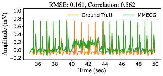
(a)

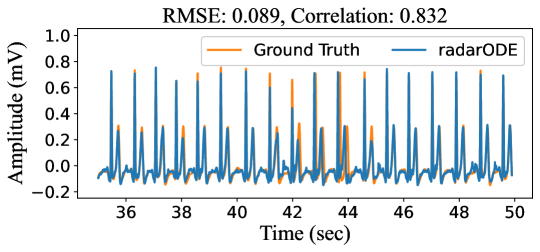
(b)

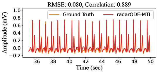
(c)

Figure 5: Illustration of different frameworks under the same abrupt RBM noise: (a) MMECG cannot provide reasonable recovery under the noise; (b) radarODE could provide the general ECG shape but with a misalignment issue; (c) radarODE-MTL generates the high-fidelity ECG recovery under the noise.

To conclude the above evaluations in terms of different tasks, the proposed EGA could successfully alleviate the gradient conflicts and magnitude dominance in MTL optimization, while the intrinsic task difficulty can be successfully estimated to guide the optimization direction by introducing eccentric vector $\boldsymbol{v}_{ecc}$. Compared with other methods, EGA achieves an outstanding result for the tasks with disparate difficulties and is also competitive in the common tasks, but the hyperparameter $T$ should be carefully selected with large $T$ evenly treating all the tasks and small $T$ highlighting the hard task in each training epoch.

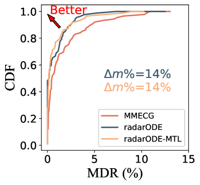
(a)

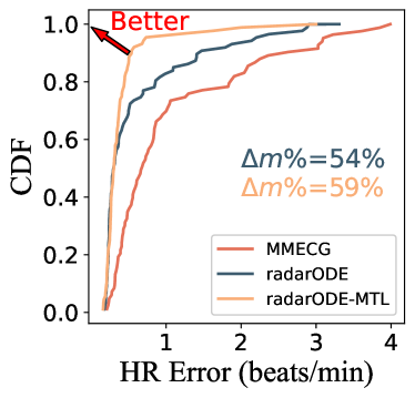
(b)

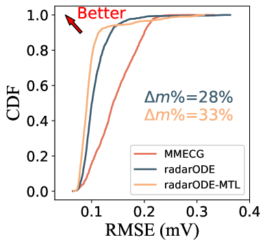
(c)

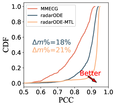
(d)

Figure 6: Evaluations for long-term ECG recovery: (a) - (d) CDF plots of MDR, HR Error, RMSE and PCC, with corresponding improvements.

IV-C Evaluations on the Long-term Recovered ECG

The outputs from Task $1-3$ can form the long-term ECG signal as introduced in Methodology and the general performance can be depicted in Figure 5, with all three frameworks successfully reconstructing the ECG signals without noises. However, Figure LABEL:sub@fig:mmecg_noise shows that MMECG cannot resist RBM noise and obtains bad RMSE/PCC as also reported in the benchmark paper [2]. In contrast, radarODE could preserve the general shapes of ECG pieces due to the constrain from ODE model [5], but the peaks deviate from the ground truth because the inaccurate PPI estimation and the reintroduction of noises in long-term reconstruction stage, degrading the RMSE/PCC as shown in Figure LABEL:sub@fig:ode_noise. Lastly, the proposed radarODE-MTL realizes the ECG reconstruction in an end-to-end manner without reintroducing the noises, and the recovered ECG is less corrupted by the noises with the best RMSE/PCC compared with other frameworks as shown in Figure LABEL:sub@fig:mtl_noise. The following part will thoroughly evaluate the recovered long-term ECG signals in terms of corrupt ECG reconstruction, coarse cardiac feature and fine-grained ECG feature reconstruction, respectively.

IV-C1 Corrupt ECG Reconstruction

The concept of MDR is used to statistically evaluate the corruptions in the recovered ECG signals due to noise distortion. The result is shown as the cumulative distribution function (CDF) of MDR in Figure LABEL:sub@fig:mdr_cdf with the median MDR as $1.7\%$, $0.13\%$ and $0.13\%$ for MMECG, radarODE and radarODE-MTL respectively, and $\Delta m\%$ across $91$ trails are both $14\%$. The reason for the similar performance of two ODE-based methods is that the misaligned ECG pieces with small deviations ($<150$ms) in radarODE will not be identified as ‘missed detected’, and hence the CDFs of MDR share a similar pattern and trend in Figure LABEL:sub@fig:mdr_cdf.

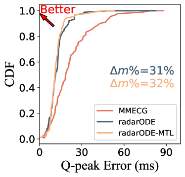
(a)

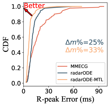
(b)

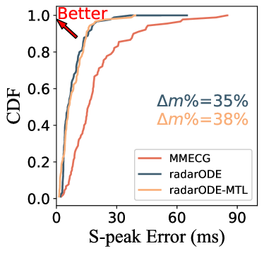
(c)

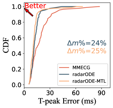
(d)

Figure 7: Evaluations for fine-grained ECG peaks recovery: (a) - (d) CDF plots of the timing error for QRST peaks, with corresponding improvements.

IV-C2 Coarse Cardiac Feature Reconstruction

All three frameworks evaluated in this paper are designed for fine-grained cardiac features reconstruction and should perform well on the coarse cardiac feature (i.e., heart rate (HR) monitoring). The result in Figure LABEL:sub@fig:hr_cdf coincides with the expectation with median HR error as $0.6$, $0.3$ and $0.3$ beats/min respectively, and $\Delta m\%$ for the ODE-based methods are $43\%$ and $48\%$. It is notable in Figure LABEL:sub@fig:hr_cdf that the performances of ODE-based methods are very similar at the beginning, while the radarODE tends to get more errors when the noise in the raw radar signal affects the R peaks recovery, because the calculation of HR is based on the R peak positions.

IV-C3 Fine-Grained Morphological Feature Reconstruction

The morphological feature is an essential fine-grained feature to describe the general similarity between the recovered and ground truth ECG signals, and the morphological accuracy can be evaluated by RMSE and PCC, with RMSE sensitive to the peak deviation and PCC focusing on the similarity of the general shape. The results are shown in Figure LABEL:sub@fig:rmse_cdf and LABEL:sub@fig:ocor_cdf as the CDF of RMSE/PCC across $91$ trails in the dataset, and three frameworks get the median RMSE/PCC as $0.125$mV/$82.1\%$, $0.098$mV/$90.1\%$ and $0.083$mV/$92.7\%$ respectively. As indicated by $\Delta m\%$, the improvements of RMSE ($28\%,33\%$) are larger than PCC ($18\%,21\%$) for radarODE and radarODE-MTL respectively, because the ODE model embedded in the decoder preserves the main features of ECG even under noises and contributes more on the peaks than on the shapes. In addition, radarODE-MTL further improves the results by aligning the ECG pieces with the predicted anchors, avoiding the misalignment issue in radarODE.

IV-C4 Fine-Grained ECG Peaks Reconstruction

In the evaluations of timing errors of the ECG peaks it is common only to analyze QRST peaks because the inconspicuous P peaks can be miss-detected even in some ground truth signals [2, 5]. The CDF plots for the absolute timing errors of QRST peaks are shown in Figure 7 with the following observations:

• Both ODE-based methods reveal better performance than the benchmark, but the radarODE-MTL only achieves equivalent performance as radarODE with similar $\Delta m\%$ around $31\%$, $35\%$ and $24\%$ as shown in Figure LABEL:sub@fig:Q_cdf, LABEL:sub@fig:S_cdf and LABEL:sub@fig:T_cdf. The possible reason is that radarODE-MTL only aligns the ECG pieces with R peaks, but the impacts on the QST peaks are random. In other words, the alignment of the R peak may degrade the accuracy of other peaks, and hence the overall performance of radarODE and radarODE-MTL on the QST peaks are similar.

• It is worth noticing that $\Delta m\%$ of the radarODE-MTL ($33\%$) on the R peak is obviously larger than that of the radarODE ($25\%$), with the median timing error as $14$, $10$ and $6$ms for three frameworks as shown in Figure LABEL:sub@fig:R_cdf. Therefore, radarODE-MTL is a better way to generate long-term ECG signals by aligning the ECG pieces with predicted R peaks, instead of reintroducing the noisy time-domain radar signal as in radarODE.

IV-D Noise Robustness Test

In this work, $10$ trails (No. $75-84$) are selected for the noise robustness test by adding different types of synthesized noises with certain decibel (dB).

IV-D1 Constant Noise

The constant noise normally affects the SNR of the signal, and can be simulated by adding Gaussian noise with different intensities as implemented in [6, 19, 40, 41, 42]. The baseline results for three frameworks are firstly obtained in terms of the RMSE, PCC, R-peak error and MDR as shown in Table III, and $\Delta m\%$ is calculated as $0\%$, $7.47\%$ and $10.64\%$ as indicated by the initial points in Figure 8. Then, the Gaussian noises with $6$ to $-3$dB are added into the raw radar signal without retraining the deep-learning framework, and the results are shown in Table III with the trends of performance degradation shown in Figure 8.

TABLE III: Comparison of the frameworks under different SNR

SNR	RMSE (mV) $\downarrow$	PCC $\uparrow$	Peak Error (ms) $\downarrow$	MDR $\downarrow$	$\Delta m\%^{1}\uparrow$
MMECG [2]
Baseline	0.107	83.75%	9.45	4.52%	0.0%
${\color[rgb]{1,1,1}-}6$ dB	0.107	82.60%	9.76	4.37%	-0.44%
${\color[rgb]{1,1,1}-}3$ dB	0.108	82.64%	9.85	4.84%	-3.20%
${\color[rgb]{1,1,1}-}0$ dB	0.109	80.00%	11.80	4.92%	-10.14%
$-1$ dB	0.114	78.55%	12.20	5.32%	-15.02%
$-2$ dB	0.120	74.32%	14.64	5.59%	-25.42%
$-3$ dB	0.127	62.45%	21.28	6.40%	-52.82%
radarODE [5]
Baseline	0.091	83.53%	9.08	4.03%	0.0%
${\color[rgb]{1,1,1}-}6$ dB	0.093	83.30%	9.12	4.36%	-2.83%
${\color[rgb]{1,1,1}-}3$ dB	0.095	83.01%	9.01	4.70%	-5.23%
${\color[rgb]{1,1,1}-}0$ dB	0.101	82.21%	9.89	5.86%	-16.86%
$-1$ dB	0.116	79.66%	11.90	5.36%	-24.17%
$-2$ dB	0.157	70.87%	13.95	6.19%	-48.74%
$-3$ dB	-	-	-	-	Failed2
radarODE-MTL
Baseline	0.089	85.03%	8.22	4.08%	0.0%
${\color[rgb]{1,1,1}-}6$ dB	0.088	85.31%	8.18	4.20%	-0.31%
${\color[rgb]{1,1,1}-}3$ dB	0.089	84.29%	8.31	4.27%	-1.87%
${\color[rgb]{1,1,1}-}0$ dB	0.091	83.77%	8.03	4.76%	-4.58%
$-1$ dB	0.093	84.01%	8.10	5.10%	-7.33%
$-2$ dB	0.093	84.51%	8.02	5.45%	-9.18%
$-3$ dB	0.094	84.96%	8.19	6.02%	-13.30%
1. $\Delta m\%$ is calculated for each framework based on each baseline.
2. The ECG recovery fails if PCC$<60\%$, according to the empirical
observation of the morphological ECG features.

A general observation of Table III is that all the frameworks perform well before $0$dB with a similar degradation rate as in Figure LABEL:sub@fig:constant. Then, radarODE-MTL could still provide reasonable results with mild degradation after $0$dB because the MTL paradigm split the ECG reconstruction task into several sub-tasks, and each task can either be constrained by prior knowledge or leverage the information from context data with less pollution. In contrast, radarODE could generate high-fidelity ECG pieces as claimed in [5] and gets the second best baseline result in Table III, but the design of PPI estimation stage does not consider the noise robustness. Therefore, the performance is heavily dropped to the worst in Figure LABEL:sub@fig:constant because of the bad results of Peak Error as shown in Table III. Lastly, the MMECG considers the ECG recovery as an arbitrary domain transformation problem without any constraints in the network design, and the performance also heavily degrades in Figure LABEL:sub@fig:constant because only meaningless results will be generated as shown previously in Figure LABEL:sub@fig:mmecg_noise.

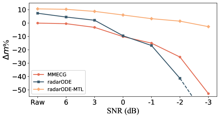
(a)

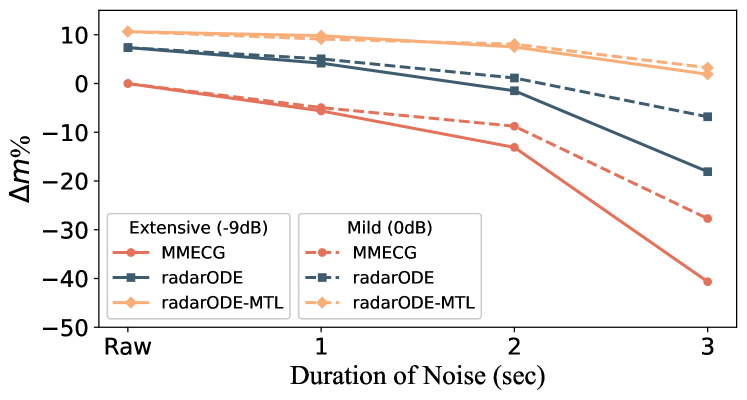
(b)

Figure 8: Noise robustness test: (a) Impact of constant noises with different intensities, (b) Impact of abrupt noises with different intensities and durations.

TABLE IV: Comparison of the frameworks under abrupt noises

Duration	RMSE (mV) $\downarrow$	PCC $\uparrow$	Peak Error (ms) $\downarrow$	MDR $\downarrow$	$\Delta m\%^{1}\uparrow$	RMSE (mV) $\downarrow$	PCC $\uparrow$	Peak Error (ms) $\downarrow$	MDR $\downarrow$	$\Delta m\%\uparrow$
MMECG [2]:	Mild Body Movement ($0$ dB)					Extensive Body Movement ($-9$ dB)
Baseline	0.107	83.75%	9.45	4.52%	0.0%	0.107	83.75%	9.45	4.52%	0.0%
$1$ sec	0.107	85.53%	10.84	4.82%	-4.94%	0.107	84.05%	10.93	4.82%	-5.62%
$2$ sec	0.110	82.64%	11.31	5.02%	-8.76%	0.108	79.01%	12.31	5.23%	-13.10%
$3$ sec	0.114	76.87%	15.56	5.92%	-27.71%	0.116	75.09%	12.50	9.56%	-40.66%
radarODE [5]:	Mild Body Movement ($0$ dB)					Extensive Body Movement ($-9$ dB)
Baseline	0.091	83.53%	9.08	4.03%	0.0%	0.091	83.53%	9.08	4.03%	0.0%
$1$ sec	0.091	83.49%	9.12	4.36%	-2.31%	0.095	82.96%	9.15	4.33%	-3.19%
$2$ sec	0.092	83.39%	9.82	4.64%	-6.23%	0.098	82.16%	9.31	4.97%	-8.86%
$3$ sec	0.095	83.01%	10.01	5.7%	-14.19%	0.102	81.87%	9.66	7.39%	-25.46%
radarODE-MTL:	Mild Body Movement ($0$ dB)					Extensive Body Movement ($-9$ dB)
Baseline	0.089	85.03%	8.22	4.08%	0.0%	0.089	85.03%	8.22	4.08%	0.0%
$1$ sec	0.090	84.62%	7.87	4.42%	-1.52%	0.090	84.31%	8.28	4.08%	-0.82%
$2$ sec	0.090	84.78%	8.29	4.44%	-2.56%	0.091	84.21%	8.32	4.41%	-3.15%
$3$ sec	0.091	84.44%	8.34	5.12%	-7.39%	0.095	84.17%	8.43	5.10%	-8.74%
1. $\Delta m\%$ is calculated for each framework based on the corresponding baseline.

IV-D2 Abrupt Noise

In this part, the Gaussian noises with different intensities ($0$ and $-9$dB) are used to simulate mild body movement (e.g., during talking or writing) and extensive body movement (e.g., during torso movement) as suggested in the literature [43]. Only $20\%$ of the segments randomly selected from one trial are doped, and the duration of noise varies from $1$ to $3$ sec.

For mild body movement, the experimental results are shown in Table IV with the changes of $\Delta m\%$ shown in Figure LABEL:sub@fig:abrupt. Firstly, it is evident that the impact of $1$-sec abrupt noise is limited for all the frameworks, and the results for ODE-based methods are almost equivalent to the baselines. Secondly, $2$-sec noise starts to have a noticeable impact on MMECG, while the ODE-based methods could preserve the performance on the morphological features (RMSE/PCC) with small degradation on the Peak Error and MDR. Lastly, $3$-sec noise has distorted $3/4$ of the input radar segment, and the performances of MMECG and radarODE drop obviously as shown in Figure LABEL:sub@fig:abrupt, while radarODE-MTL only loses some points on $\text{MDR}=5.12\%$ as shown in Table IV.

In comparison, the extensive body movements with $1$ and $2$ sec have similar impacts with mild ones on ODE-based methods, because the ODE decoder could preserve the ECG shape even under strong noises, whereas the segments affected by noise cannot contribute to the recovery for MMECG as evident by the significant drop of PCC (from $84.05\%$ to $79.01\%$) as shown in Table IV. In addition, the $3$-sec noise destroys the ECG recovery for MMECG and radarODE with a significant degradation as shown in Figure LABEL:sub@fig:abrupt, whereas the radarODE-MTL only sacrifices certain RMSE and peak accuracy with the overall degradation dropping slightly from $-7.39\%$ to $-8.74\%$ as shown in Table IV.

In summary, the noise-robustness tests indicate that it is necessary to consider the noise robustness when designing the deep-learning model, because both MMECG and radarODE reveal a severe degradation in the performance, especially for the low SNR scenarios. In addition, the deconstruction of the ECG recovery task in radarODE-MTL could effectively resist the noises, because the ODE decoder protects the morphological feature, and the peak accuracy can be compensated from the adjacent cardiac cycles with less noise distortion.

V Conclusions

This paper investigates the radar-based ECG monitoring technique and proposes a deep-learning framework radarODE-MTL to provide accurate ECG monitoring under noises. The radarODE-MTL adopts the MTL paradigm to realize the ECG reconstruction through $3$ sub-tasks, and a novel optimization strategy called EGA is also proposed to simultaneously optimize all the tasks without stall or negative transfer issues. The performance of EGA has been evaluated on various MTL tasks, and the experimental results evidence that EGA is competitive with other state-of-the-art optimization strategies on the unified task and achieves outstanding results on radar-based EGA recovery with unbalanced task difficulties. In addition, the well-trained radarODE-MTL could provide long-term ECG reconstructions with high fidelity in terms of MDR, morphological similarity and peak accuracy. Lastly, this is the first study that conducts noise-robustness tests for deep-learning frameworks, and the proposed radarODE-MTL could also achieve reasonable ECG recovery with mild degradation under constant and abrupt noises. In the future, the proposed method needs to be verified for patients with cardiovascular diseases to enable potential clinical use.

References

- [1] L. M. Swift, M. W. Kay, C. M. Ripplinger, and N. G. Posnack, “Stop the beat to see the rhythm: excitation-contraction uncoupling in cardiac research,” American Journal of Physiology-Heart and Circulatory Physiology, vol. 321, no. 6, pp. H1005–H1013, Dec. 2021.
- [2] J. Chen, D. Zhang, Z. Wu, F. Zhou, Q. Sun, and Y. Chen, “Contactless electrocardiogram monitoring with millimeter wave radar,” IEEE Transactions on Mobile Computing, Dec. 2022.
- [3] Y. Wu, H. Ni, C. Mao, and J. Han, “Contactless reconstruction of ECG and respiration signals with mmWave Radar based on RSSRnet,” IEEE Sensors Journal, Nov. 2023.
- [4] Z. Wang, B. Jin, S. Li, F. Zhang, and W. Zhang, “ECG-grained cardiac monitoring using UWB signals,” Proceedings of the ACM on Interactive, Mobile, Wearable and Ubiquitous Technologies, vol. 6, no. 4, pp. 1–25, Dec. 2023.
- [5] Y. Zhang, R. Guan, L. Li, R. Yang, Y. Yue, and E. G. Lim, “radarODE: An ODE-embedded deep learning model for contactless ECG reconstruction from millimeter-wave radar,” arXiv preprint arXiv:2408.01672 [eess], Aug. 2024.
- [6] S. Dong, Y. Li, C. Gu, and J. Mao, “Robust cardiac timing detection technique with vectors analytic demodulation in Doppler cardiogram sensing,” IEEE Transactions on Microwave Theory and Techniques, Jan. 2024.
- [7] S. Ji, Z. Zhang, Z. Xia, H. Wen, J. Zhu, and K. Zhao, “RBHHM: A novel remote cardiac cycle detection model based on heartbeat harmonics,” Biomedical Signal Processing and Control, vol. 78, p. 103936, Sep. 2022.
- [8] W. Xia, Y. Li, and S. Dong, “Radar-based high-accuracy cardiac activity sensing,” IEEE Transactions on Instrumentation and Measurement, vol. 70, pp. 1–13, Jan. 2021.
- [9] D. Makowski, T. Pham, Z. J. Lau, J. C. Brammer, F. Lespinasse, H. Pham, C. Schölzel, and S. A. Chen, “NeuroKit2: A Python toolbox for neurophysiological signal processing,” Behavior Research Methods, pp. 1–8, Feb. 2021.
- [10] B. Lin and Y. Zhang, “LibMTL: A Python library for multi-task learning,” Journal of Machine Learning Research, vol. 24, no. 209, pp. 1–7, Jul. 2023.
- [11] R. Guan, R. Zhang, N. Ouyang, J. Liu, K. L. Man, X. Cai, M. Xu, J. Smith, E. G. Lim, Y. Yue et al., “Talk2radar: Bridging natural language with 4D mmwave radar for 3D referring expression comprehension,” arXiv preprint arXiv:2405.12821, Jul. 2024.
- [12] N. Silberman, D. Hoiem, P. Kohli, and R. Fergus, “Indoor segmentation and support inference from RGBD images,” in Proceedings of the European Conference on Computer Vision. Springer, Oct. 2012, pp. 746–760.
- [13] C. Yeshwanth, Y.-C. Liu, M. Nießner, and A. Dai, “Scannet++: A high-fidelity dataset of 3D indoor scenes,” in Proceedings of the IEEE/CVF International Conference on Computer Vision, Oct. 2023, pp. 12–22.
- [14] S. Yao, R. Guan, Z. Wu, Y. Ni, Z. Zhang, Z. Huang, X. Zhu, Y. Yue, E. G. Lim, H. Seo et al., “Waterscenes: A multi-task 4D radar-camera fusion dataset and benchmark for autonomous driving on water surfaces,” IEEE Transactions on Intelligent Transportation Systems, Jul. 2023.
- [15] L.-Y. Liu, W.-Z. Liu, and L. Feng, “A primary task driven adaptive loss function for multi-task speech emotion recognition,” Engineering Applications of Artificial Intelligence, vol. 127, p. 107286, Jan 2024.
- [16] M. Guo, A. Haque, D.-A. Huang, S. Yeung, and L. Fei-Fei, “Dynamic task prioritization for multitask learning,” in Proceedings of the European Conference on Computer Vision, Sep. 2018, pp. 270–287.
- [17] H. Shen, C. Xu, Y. Yang, L. Sun, Z. Cai, L. Bai, E. Clancy, and X. Huang, “Respiration and heartbeat rates measurement based on autocorrelation using IR-UWB radar,” IEEE Transactions on Circuits and Systems II: Express Briefs, vol. 65, no. 10, pp. 1470–1474, Oct. 2018.
- [18] M. Lin, R. Chi, and N. Sheng, “Data driven latent variable adaptive control for nonlinear multivariable processes,” International Journal of Systems Science, pp. 1–18, Aug. 2024.
- [19] J. Liu, J. Wang, Q. Gao, X. Li, M. Pan, and Y. Fang, “Diversity-enhanced robust device-free vital signs monitoring using mmWave signals,” IEEE Transactions on Mobile Computing, Jun. 2024.
- [20] R. Caruana, “Multitask learning: A knowledge-based source of inductive bias,” in Proceedings of the Tenth International Conference on Machine Learning. Citeseer, 1993, pp. 41–48.
- [21] D. Senushkin, N. Patakin, A. Kuznetsov, and A. Konushin, “Independent component alignment for multi-task learning,” in Proceedings of the IEEE/CVF Conference on Computer Vision and Pattern Recognition, Sep. 2023, pp. 20 083–20 093.
- [22] H. Fernando, H. Shen, M. Liu, S. Chaudhury, K. Murugesan, and T. Chen, “Mitigating gradient bias in multi-objective learning: A provably convergent approach,” in International Conference on Learning Representations, May 2023.
- [23] L. Liu, Y. Li, Z. Kuang, J.-H. Xue, Y. Chen, W. Yang, Q. Liao, and W. Zhang, “Towards impartial multi-task learning,” in International Conference on Learning Representations, Oct. 2021.
- [24] B. Liu, X. Liu, X. Jin, P. Stone, and Q. Liu, “Conflict-averse gradient descent for multi-task learning,” Advances in Neural Information Processing Systems, vol. 34, pp. 18 878–18 890, Dec. 2021.
- [25] X. Lin, X. Zhang, Z. Yang, F. Liu, Z. Wang, and Q. Zhang, “Smooth Tchebycheff scalarization for multi-objective optimization,” in International Conference on Machine Learning, Jul. 2024.
- [26] S. Liu, E. Johns, and A. J. Davison, “End-to-end multi-task learning with attention,” in Proceedings of the IEEE/CVF Conference on Computer Vision and Pattern Recognition, Jun. 2019, pp. 1871–1880.
- [27] S. Chennupati, G. Sistu, S. Yogamani, and S. A Rawashdeh, “Multinet++: Multi-stream feature aggregation and geometric loss strategy for multi-task learning,” in Proceedings of the IEEE/CVF Conference on Computer Vision and Pattern Recognition Workshops, Nov. 2019, pp. 0–0.
- [28] A. Kendall, Y. Gal, and R. Cipolla, “Multi-task learning using uncertainty to weigh losses for scene geometry and semantics,” in Proceedings of the IEEE Conference on Computer Vision and Pattern Recognition, Jun. 2018, pp. 7482–7491.
- [29] Z. Chen, V. Badrinarayanan, C.-Y. Lee, and A. Rabinovich, “Gradnorm: Gradient normalization for adaptive loss balancing in deep multitask networks,” in International Conference on Machine Learning. PMLR, Jul. 2018, pp. 794–803.
- [30] J. Huo, L. Wang, Z. Lu, and X. Wen, “Vehicular crowdsensing inference and prediction with multi-task pre-training graph transformer networks,” IEEE Internet of Things Journal, Aug. 2023.
- [31] Y. Yao, L. Rosasco, and A. Caponnetto, “On early stopping in gradient descent learning,” Constructive Approximation, vol. 26, no. 2, pp. 289–315, Apr. 2007.
- [32] X. Chen, R. Yang, Y. Xue, B. Song, and Z. Wang, “TFPred: Learning discriminative representations from unlabeled data for few-label rotating machinery fault diagnosis,” Control Engineering Practice, vol. 146, p. 105900, Feb. 2024.
- [33] J. Wang, Y. Zhuang, and Y. Liu, “FSS-Net: A fast search structure for 3D point clouds in deep learning,” International Journal of Network Dynamics and Intelligence, pp. 100 005–100 005, Jun. 2023.
- [34] Z. Chu, R. Yan, and S. Wang, “Vessel turnaround time prediction: A machine learning approach,” Ocean & Coastal Management, vol. 249, p. 107021, Mar. 2024.
- [35] X. Dong, R. Wu, C. Xiong, H. Li, L. Cheng, Y. He, S. Qian, J. Cao, and L. Mo, “Gdod: Effective gradient descent using orthogonal decomposition for multi-task learning,” in Proceedings of the 31st ACM International Conference on Information & Knowledge Management, Oct. 2022, pp. 386–395.
- [36] P. H. Schönemann, “A generalized solution of the orthogonal Procrustes problem,” Psychometrika, vol. 31, no. 1, pp. 1–10, Mar. 1966.
- [37] I. Loshchilov and F. Hutter, “SGDR: Stochastic gradient descent with warm restarts,” arXiv preprint arXiv:1608.03983, Aug. 2016.
- [38] D. P. Kingma and J. Ba, “Adam: A method for stochastic optimization,” arXiv preprint arXiv:1412.6980, 2014.
- [39] W. Jeong and K.-J. Yoon, “Quantifying task priority for multi-task optimization,” in Proceedings of the IEEE/CVF Conference on Computer Vision and Pattern Recognition, Jun. 2024, pp. 363–372.
- [40] Y. Feng, X. Li, D. Shi, and D. Dai, “An efficient robust model predictive control for nonlinear markov jump systems with persistent disturbances using matrix partition,” International Journal of Systems Science, vol. 54, no. 10, pp. 2118–2133, May 2023.
- [41] X. Qian and B. Cui, “A mobile sensing approach to distributed consensus filtering of 2d stochastic nonlinear parabolic systems with disturbances,” Systems Science & Control Engineering, vol. 11, no. 1, p. 2167885, Jan. 2023.
- [42] Y. Xue, R. Yang, X. Chen, Z. Tian, and Z. Wang, “A novel local binary temporal convolutional neural network for bearing fault diagnosis,” IEEE Transactions on Instrumentation and Measurement, Jul. 2023.
- [43] Z. Chen, T. Zheng, C. Cai, and J. Luo, “MoVi-Fi: Motion-robust vital signs waveform recovery via deep interpreted RF sensing,” in Proceedings of the 27th Annual International Conference on Mobile Computing and Networking (MobiCom), Feb. 2021, pp. 392–405.