Riemannian Gradient Descent Method to Joint Blind Super-Resolution and Demixing in ISACthanks: Corresponding author: Jinchi Chen

Zeyu Xiang1, Haifeng Wang2, Jiayi Lv1, Yujie Wang1, Yuxue Wang1, Yuxuan Ma1, Jinchi Chen1 1School of Mathematics, East China University of Science and Technology, Shanghai, China
{jcchen.phys}@gmail.com
2China Mobile (Zhejiang) Research & Innovation Institute, Hangzhou, China
{wanghaifeng40}@zj.chinamobile.com
Abstract

Integrated Sensing and Communication (ISAC) has emerged as a promising technology for next-generation wireless networks. In this work, we tackle an ill-posed parameter estimation problem within ISAC, formulating it as a joint blind super-resolution and demixing problem. Leveraging the low-rank structures of the vectorized Hankel matrices associated with the unknown parameters, we propose a Riemannian gradient descent (RGD) method. Our theoretical analysis demonstrates that the proposed method achieves linear convergence to the target matrices under standard assumptions. Additionally, extensive numerical experiments validate the effectiveness of the proposed approach.

Index Terms:
Blind dimixing, blind super-resolution, vectorized Hankel lift, Riemannian gradient descent.

I Introduction

ISAC represents an innovative and emerging paradigm aimed at enhancing spectral efficiency by enabling the joint utilization of spectrum resources for both communication and sensing functionalities [1, 2, 3]. By integrating these two functions, ISAC seeks to reduce spectrum congestion and improve the overall performance of wireless systems.

In practical implementations of ISAC, several significant challenges arise. One major challenge is that the transmitted waveform in passive [4, 5] or multistatic [6] radar systems is often unknown to the receiver. This uncertainty complicates the ability of the receiver to effectively detect and process signals, leading to a decrease in system performance.

Another critical challenge in ISAC systems is the acquisition of accurate channel state information (CSI) in communication systems, which is inherently complex. For example, in Terahertz (THz) band communication systems [7, 1], the channel coherence time is extremely short, making it difficult to obtain reliable CSI using conventional pilot-based methods. The rapid variability of THz channels, combined with severe path loss and molecular absorption, further complicates the acquisition process.

In this paper, we consider a generalized scenario where both the radar and communication channels, along with their transmitted signals, are unknown to the common receiver. We formulate the task of estimating channel parameters and transmitted signals as a Joint Blind Super-resolution and Demixing (JBSD) problem. Specifically, we use a subspace lifting technique to leverage the low-dimensional structures inherent in the data matrices related to the channel parameters and transmitted signals. This allows us to frame the JBSD problem as a low-rank matrix demixing problem. To solve the low-rank matrix demixing problem, we propose a novel Riemannian gradient descent framework. This approach enables computationally efficient reconstruction, with exact recovery guarantees established under standard assumptions.

II Problem Formulation

Consider a scenario involving $K$ radar or communication users transmitting signals to a common receiver. The received signal at the receiver is modeled as a superposition of convolutions from $K$ users, expressed mathematically as:

$\displaystyle y(t)=\sum_{k=1}^{K}\sum_{p=1}^{r_{k}}d_{k,p}\delta(t-\tau_{k,p})\ast g_{k}(t),$

where $r_{k}$ represents the number of paths for the $k$-th user, $\tau_{k,p}\in[0,1)$ denotes the delay, $d_{k,p}$ is the complex-valued amplitude, and $g_{k}(t)$ is the waveform corresponding to the $k$-th user. By taking the Fourier transform and sampling, we obtain for $j=0,1,\cdots,n$:

$\displaystyle y[j]=\sum_{k=1}^{K}\sum_{p=1}^{r}d_{k,p}e^{-\imath 2\pi(j-1)\tau_{k,p}}\hat{g}_{k}[j],$ (II.1)

where $\hat{g}_{k}$ represents the Fourier transform of $g_{k}(t)$. Defining $\bm{g}_{k}=\begin{bmatrix}g_{k}[0]&\cdots&g_{k}[n-1]\end{bmatrix}^{\mathsf{T}}\in\mathbb{C}^{n}$, the objective of the JBSD problem is to estimate the parameters $\{d_{k,p},\tau_{k,p}\}$ as well as the unknown signals $\{\bm{g}_{k}\}$ from the observations in the equation above.

Since the number of measurements is less than the number of unknowns, JBSD is an ill-posed problem. To address this challenge, we adopt a subspace assumption inspired by prior research [8, 9, 10, 11]. Specifically, we assume that each signal $\bm{g}_{k}$ lies in a low-dimensional subspace defined by a matrix $\bm{B}_{k}\in\mathbb{C}^{n\times s_{k}}$, such that

$\displaystyle\bm{g}_{k}=\bm{B}_{k}\bm{h}_{k},\quad p=1,\cdots,r.$

where $\bm{h}_{k}\in\mathbb{C}^{s_{k}}$ is an unknown coefficient vector. This assumption implies that the waveform $\bm{g}_{k}$ can be represented as a linear combination of a redundant codebook matrix $\bm{B}_{k}$.

Under the subspace assumption, the measurements can be expressed as:

$\displaystyle y[j]=\sum_{k=1}^{K}\left\langle\bm{b}_{k,j}\bm{e}_{j}^{\mathsf{T}},\bm{X}_{k,\natural}\right\rangle,$ (II.2)

where $\bm{X}_{k,\natural}=\sum_{p=1}^{r_{k}}d_{k,p}\bm{h}_{k}\bm{a}_{\tau_{k,p}}^{\mathsf{T}}$, the steering vector $\bm{a}_{\tau}\in\mathbb{C}^{n}$ is defined by:

$\displaystyle\begin{bmatrix}1&e^{-\imath 2\pi\tau}&\cdots&e^{-\imath 2\pi\tau(n-1)}\end{bmatrix}^{\mathsf{T}},$

and $\left\langle\cdot,\cdot\right\rangle$ represents the inner product, defined as $\left\langle\bm{A},\bm{B}\right\rangle=\operatorname{trace}(\bm{A}^{\mathsf{H}}\bm{B})$. Without loss of generality, we assume $r_{1}=\cdots=r_{K}=r$ and $s_{1}=\cdots=s_{K}=s$. Let ${\cal A}_{k}:\mathbb{C}^{s\times n}\rightarrow\mathbb{C}^{n}$ be a linear operator defined by:

$\displaystyle{\cal A}_{k}(\bm{X})[j]=\left\langle\bm{b}_{k,j}\bm{e}_{j}^{\mathsf{T}},\bm{X}\right\rangle,$

with the adjoint operator ${\cal A}^{\ast}_{k}$ given by ${\cal A}^{\ast}_{k}(\bm{y})=\sum_{j=1}^{n}\bm{y}[j]\bm{b}_{j,k}\bm{e}_{j}^{\mathsf{T}}$. Then the measurements in can be expressed as a more compact form:

$\displaystyle\bm{y}=\sum_{k=1}^{K}{\cal A}_{k}(\bm{X}_{k,\natural}).$ (II.3)

The problem of JBSD can thus be formulated as the task of demixing a sequence of matrices $\{\bm{X}_{k}\}$ from the superposed linear measurements. Once the data matrices are recovered, the delays $\{\tau_{k,p}\}$ can be estimated using spatial smoothing MUSIC [12, 13, 14, 15], and the parameters $\{d_{k,p},\bm{h}_{k}\}$ can be recovered using an overparameterized linear system [16]. Thus the main objective of this work is to efficiently recover the data matrices $\{\bm{X}_{k,\natural}\}$ from the measurement (II.2).

When $K=1$, JBSD reduces to the classical blind super-resolution problem. Convex and non-convex approaches have been successfully employed to solve this problem. In particular, the theoretical guarantees of convex methods, including atomic norm minimization [17, 18, 19] and nuclear norm minimization [12], have been established. However, these convex optimization-based methods are computationally expensive. To overcome this issue, non-convex optimization-based methods, such as low-rank factorization [20, 21] and low-rank manifold-based [22] approaches, have gained attention for their efficiency in leveraging the low-rank structures of the data matrices.

Given that the measurements are a superposition of multiple users’ data, JBSD presents a greater challenge compared to blind super-resolution. Consequently, theoretical guarantees and algorithms developed for blind super-resolution cannot be directly applied to JBSD. Recent research has focused on JBSD, with notable progress achieved through methods such as ANM (Atomic Norm Minimization) [8, 23, 24] and vectorized Hankel lifts[25, 26]. However, compared to blind super-resolution, computationally efficient algorithms for JBSD remain limited. Therefore, developing fast and robust algorithms for JBSD is a critical area of interest. In this work, we propose a Riemannian gradient descent method for solving the aforementioned optimization problem efficiently.

III Algorithms

Let ${\cal H}:\mathbb{C}^{s\times n}\rightarrow\mathbb{C}^{sn_{1}\times n_{2}}$ denote the vectorized Hankel lift operator defined as follows:

$\displaystyle{\cal H}(\bm{X})=\begin{bmatrix}\bm{x}_{0}&\bm{x}_{1}&\cdots&\bm{x}_{n_{2}-1}\\ \bm{x}_{1}&\bm{x}_{2}&\cdots&\bm{x}_{n_{2}}\\ \vdots&\vdots&\ddots&\vdots\\ \bm{x}_{n_{1}-1}&\bm{x}_{n_{1}}&\cdots&\bm{x}_{n-1}\\ \end{bmatrix}\in\mathbb{C}^{sn_{1}\times n_{2}},$

where $\bm{x}_{j}$ is the $(j+1)$-th column of $\bm{X}$ with $j=0,1,\cdots,n-1$, and $n_{1}+n_{2}=n+1$. It has shown that $\operatorname{\mathrm{rank}}({\cal H}(\bm{X}_{k,\natural}))=r$ [12]. Consequently, we consider the following non-convex optimization problem to recover the data matrices:

$\displaystyle\min_{\bm{X}_{k}}~{}$ $\displaystyle\frac{1}{2}\left\|\bm{D}\bm{y}-\sum_{k=1}^{K}{\cal A}_{k}{\cal D}(\bm{X}_{k})\right\|_{{\footnotesize{2}}}^{2}~{}\text{s.t.}~{}\operatorname{\mathrm{rank}}({\cal H}(\bm{X}_{k}))=r.$ (III.1)

Furthermore, we define the operator ${\cal D}:\mathbb{C}^{s\times n}\rightarrow\mathbb{C}^{s\times n}$ as follows:

$\displaystyle{\cal D}(\bm{X})=\begin{bmatrix}\sqrt{w_{0}}\bm{x}_{0}&\cdots&\sqrt{w_{n-1}}\bm{x}_{n-1}\end{bmatrix},$

where $w_{i}=\#\{j+k=i,0\leq j\leq n_{1}-,0\leq k\leq n_{2}-1\}$. Let $\bm{D}={\cal D}(\bm{I}_{n})$ and ${\cal G}={\cal H}{\cal D}^{-1}$. Denoting $\bm{Z}_{k}={\cal G}{\cal D}(\bm{X}_{k})$, the optimization (III.1) can be reformulated as follows:

$\displaystyle\min_{\bm{Z}_{k}}~{}$ $\displaystyle\frac{1}{2}\left\|\bm{D}\bm{y}-\sum_{k=1}^{K}{\cal A}_{k}{\cal G}^{\ast}(\bm{Z}_{k})\right\|_{{\footnotesize{2}}},$
s.t. $\displaystyle\bm{Z}_{k}\in{\cal M}_{k,r},~{}({\cal I}-{\cal G}{\cal G}^{\ast})(\bm{Z}_{k})=\bm{0},~{}k=1,\cdots,K.$

where ${\cal M}_{k,r}$ is the Riemannian manifold of all rank-$r$ complex matrix, embedded with inner product, the second constraint guarantees that $\bm{Z}_{k}$ has the vectorized Hankel structure. Define $\bm{Z}=(\bm{Z}_{1},\cdots,\bm{Z}_{K})$. Let ${\cal M}_{r}={\cal M}_{1,r}\times\cdots\times{\cal M}_{K,r}$ be the product manifold. We also consider the following optimization problem:

$\displaystyle\min_{\bm{Z}\in{\cal M}_{r}}f(\bm{Z}),$

where

$\displaystyle f(\bm{Z}):$ $\displaystyle=\frac{1}{2}\left\|\sum_{k=1}^{K}{\cal A}_{k}{\cal G}^{\ast}(\bm{Z}_{k}-\bm{Z}_{k,\natural})\right\|_{{\footnotesize{2}}}^{2}$
$\displaystyle\qquad+\frac{1}{2}\sum_{k=1}^{K}\left\|({\cal I}-{\cal G}{\cal G}^{\ast})(\bm{Z}_{k})\right\|_{{\footnotesize{\mathsf{F}}}}^{2},$ (III.2)

We employ the Riemannian Gradient Descent (RGD) method [27] for the problem (III), which is summarized in Algorithm 1. The RGD algorithm generates a sequence of iterates using the following update rule:

$\displaystyle\bm{Z}_{k,t+1}={\cal R}_{k}\left(\bm{Z}_{k,t}-\eta_{t}\nabla_{{\cal M}_{k,r}}f(\bm{Z}_{k,t})\right),$

where $\eta_{t}$ represents the step size, $\nabla_{{\cal M}_{k,r}}f(\bm{Z}_{k,t})$ is the Riemannian gradient at $\bm{Z}_{k,t}$, and ${\cal R}_{k}(\cdot)$ is the retraction operator. By adopting the canonical Riemannian metric and employing truncated Singular Value Decomposition (SVD) as the retraction, the RGD method becomes:

$\displaystyle\bm{Z}_{k,t+1}={\cal P}_{r}\left(\bm{Z}_{k,t}-\alpha_{t}{\cal P}_{T_{k,t}}(\bm{G}_{k,t})\right),$

where $\bm{G}_{k,t}$ is given by

$\displaystyle\bm{G}_{k,t}=\sum_{\ell=1}^{K}{\cal G}{\cal A}_{k}^{\ast}{\cal A}_{\ell}{\cal G}^{\ast}(\bm{Z}_{\ell,t}-\bm{Z}_{\ell,\natural})+({\cal I}-{\cal G}{\cal G}^{\ast})(\bm{Z}_{k,t}),$ (III.3)

and ${\cal P}_{T_{k,t}}$ represents the projection onto the tangent space of the manifold ${\cal M}_{k,r}$ at $\bm{Z}_{k,t}$. Let $\bm{Z}_{k,t}=\bm{U}_{k,t}\bm{\Sigma}_{k,t}\bm{V}_{k,t}^{\mathsf{H}}$ be the compact SVD. The tangent space $T_{k,t}$ of ${\cal M}_{k,r}$ at $\bm{Z}_{k,t}$ is defined as follows:

$\displaystyle T_{k,t}=\{\bm{U}_{k,t}\bm{A}_{k,t}^{\mathsf{H}}+\bm{B}_{k,t}\bm{V}_{k,t}^{\mathsf{H}}:\bm{A}_{k,t}\in\mathbb{C}^{n_{2}\times r},\bm{B}_{k,t}\in\mathbb{C}^{sn_{1}\times r}\}.$

The projection ${\cal P}_{T_{k,t}}(\bm{Y}_{k})$ is defined as follows:

$\displaystyle{\cal P}_{T_{k,t}}(\bm{Y}_{k})=\bm{U}_{k,t}\bm{U}_{k,t}^{\mathsf{H}}\bm{Y}_{k}+\bm{Y}_{k}\bm{V}_{k,t}\bm{V}_{k,t}^{\mathsf{H}}-\bm{U}_{k,t}\bm{U}_{k,t}^{\mathsf{H}}\bm{Y}_{k}\bm{V}_{k,t}\bm{V}_{k,t}^{\mathsf{H}}.$

Indeed, the RGD algorithm can be regarded as a generalization of Fast Iterative Hard Thresholding (FIHT) in [28, 29, 22] to the JBSD problem. Moreover, the RGD method can be efficiently implemented, where the main computational complexity in each step is ${\cal O}(K(r^{2}sn+r^{3}+srn\log n))$.

1
2for $t=0,1,\cdots,T-1$ do
       // Fully parallel
3       for $k=1,\cdots,K$ do
4             Compute the gradient $\bm{G}_{k,t}$ via (III.3);
5             Update on the tangent space: $\bm{W}_{k,t}=\bm{Z}_{k,t}-\alpha_{t}{\cal P}_{T_{k,t}}(\bm{G}_{k,t})$;
6             Retaction: $\bm{Z}_{k,t+1}={\cal P}_{r}(\bm{W}_{k,t})$;
7            
8       end for
9      
10 end for
11
Algorithm 1 RGD–JBSD

IV Theoretical Results

In this section, we present our primary result based on the following two assumptions.

Assumption IV.1 ($\mu_{0}$-incoherence).

Suppose that the columns $\{\bm{b}_{k,i}\}$ of $\bm{B}_{k}^{\mathsf{H}}$ for $k=1,\cdots,K$, are i.i.d sampled from the a distribution $F$, which satisfies the following conditions for $\bm{b}\sim F$:

$\displaystyle\mathbb{E}\left\{\bm{b}\rule{0.0pt}{8.53581pt}\right\}=\bm{0},\mathbb{E}\left\{\bm{b}\bm{b}^{\mathsf{H}}\rule{0.0pt}{8.53581pt}\right\}=\bm{I},\max_{1\leq p\leq s}|\bm{b}[p]|\leq\sqrt{\mu_{0}}.$
Assumption IV.2 ($\mu_{1}$-incoherence).

Let $\bm{Z}_{k,\natural}=\bm{U}_{k,\natural}\bm{\Sigma}_{k,\natural}\bm{V}_{k,\natural}^{\mathsf{H}}$ be the singular value decomposition of $\bm{Z}_{k,\natural}$, where $\bm{U}_{k,\natural}\in\mathbb{C}^{sn_{1}\times r},\bm{V}_{k,\natural}\in\mathbb{C}^{n_{2}\times r}$. Let $\bm{U}_{k,\natural,j}=\bm{U}_{k,\natural}[js:(j+1)s-1,:]\in\mathbb{C}^{s\times r}$ be the $j$-th block of $\bm{U}_{k,\natural}$ for $j=0,\cdots,n_{1}-1$. Suppose that for all $k=1,\cdots,K$, the matrix $\bm{Z}_{k,\natural}$ obeys the following conditions:

$\displaystyle\max_{0\leq j\leq n_{1}-1}\left\|\bm{U}_{k,\natural,j}\right\|_{{\footnotesize{\mathsf{F}}}}^{2}\leq\frac{\mu_{1}r}{n}\text{ and }\max_{0\leq\ell\leq n_{2}-1}\left\|\bm{e}_{\ell}^{\mathsf{T}}\bm{V}_{k,\natural}\right\|_{{\footnotesize{2}}}^{2}\leq\frac{\mu_{1}r}{n}$

for some positive constant $\mu_{1}$.

We are now prepared to formally state our main result.

Theorem IV.1.

Assume that Assumptions IV.1 and IV.2 hold. If the number of measurements satisfies $n\geq C_{\gamma}K^{2}s^{2}r^{2}\kappa^{2}\mu_{0}^{2}\mu_{1}\log^{2}(sn)$, then with probability at least $1-(sn)^{-\gamma}$, the iterations produced by Algorithm 1 satisfy

$\displaystyle\sum_{k=1}^{K}\left\|\bm{Z}_{k}-\bm{Z}_{k,\natural}\right\|_{{\footnotesize{\mathsf{F}}}}^{2}\leq\frac{1}{2^{t}}\cdot\frac{\sigma_{0}^{2}}{K\mu_{0}s(1+\varepsilon)}$ (IV.1)

for $t=0,1,\cdots,T$, where $\sigma_{0}^{2}=\sum_{k=1}^{K}\sigma_{r}^{2}(\bm{Z}_{k,\natural})$ and $\kappa=\frac{\max_{k}\sigma_{1}(\bm{Z}_{k,\natural})}{\min_{k}\sigma_{r}(\bm{Z}_{k,\natural})}$.

Remark IV.1.

Theorem IV.1 establishes that RGD converges to the target matrices at a linear rate. Furthermore, the convergence rate is independent of the condition number of the target matrix, underscoring the efficiency of the proposed method.

V Numerical Experiments

In this section, we assess the performance of the proposed method and compare it to the Scaled Gradient Descent (Scaled–GD) method [16]. All numerical experiments were conducted using MATLAB R2022b on a macOS system equipped with a multi-core Intel CPU running at 2.3 GHz and 16 GB of RAM.

In our experiments, the data matrix $\bm{X}_{k,\natural}$ is constructed as $\bm{X}_{k,\natural}=\sum_{p=1}^{r}d_{k,p}\bm{h}_{k}\bm{a}_{\tau_{k,p}}^{\mathsf{T}}$. The amplitudes $\{d_{k,p}\}$ are generated in the form $(1+10^{c_{k,p}})e^{-\imath\varphi_{k,p}}$, where $c_{k,p}$ is uniformly sampled from $[0,1]$ and $\varphi_{k,p}$ is uniformly distributed over $[0,2\pi)$. The coefficient vector $\bm{h}_{k}$ is a standard Gaussian random vector, subsequently normalized. For data matrices without frequency separation, the time delay parameters $\{\tau_{k,p}\}$ are uniformly sampled from $[0,1)$. For data matrices with frequency separation, $\{\tau_{k,p}\}_{p=1,\cdots,r}$ are sampled uniformly from $[0,1)$, ensuring the minimum separation satisfies $\min_{p_{1}\neq p_{2}}|\tau_{k,p_{1}}-\tau_{k,p_{2}}|\geq\frac{1}{n}$. Additionally, the subspace matrices $\{\bm{B}_{k}\}$ are i.i.d random matrices with entries uniformly sampled from $[-\sqrt{3},\sqrt{3}]$. We conduct $20$ Monte Carlo trials and consider the recovery successful if the relative error satisfies the condition

$\displaystyle\sqrt{\frac{\sum_{k=1}^{K}\left\|\hat{\bm{X}}_{k}-\bm{X}_{k,\natural}\right\|_{{\footnotesize{\mathsf{F}}}}^{2}}{\sum_{k=1}^{K}\left\|\bm{X}_{k,\natural}\right\|_{{\footnotesize{\mathsf{F}}}}^{2}}}\leq 10^{-3}.$

The algorithms are terminated when the relative error falls below $10^{-4}$ or the number of iterations exceeds $2000$.

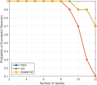
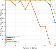
In the first experiment, we examine the recovery performance of RGD in comparison to GD and Scaled–GD using the empirical phase transition framework. We set $n=160,s=K=2$ and vary $r$ in the range $\{2:1:8\}$. Fig 1 presents the phase transition plots both with and without imposing the separation condition. The results indicate that RGD is more robust to the frequency separation condition and exhibits a higher phase transition threshold compared to the GD method.

Refer to caption
(a)
Refer to caption
(b)
Figure 1: The Empirical probability of successful recovery for RGD, GD and Scaled-GD (a) with frequency separation (b) without frequency separation.

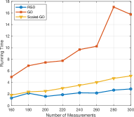
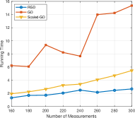
In the second experiment, we compare the running times of RGD, GD, and Scaled-GD. For this comparison, we fix the parameters $s=r=K=2$ and vary $n$ within the range $\{160:20:300\}$. We report the computational times for RGD, GD, and Scaled-GD across different values of $n$. The average computational times for all three methods are shown in Figure 2, both with and without the separation condition. The results clearly demonstrate that RGD significantly reduces running time compared to GD and Scaled-GD, particularly for larger $n$ is large, highlighting the superior efficiency of RGD.

Refer to caption
(a)
Refer to caption
(b)
Figure 2: The CPU running time for RGD, GD and Scaled-GD.

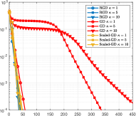
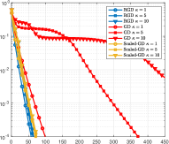
In the third experiment, we evaluate the convergence performance of RGD in comparison to GD and Saled-GD. For this comparison, we select $n=160,s=r=K=2$ and $n=256,s=r=4,K=2$. Fig 3 shows the relative recovery error as a function of iterations for different condition numbers $\kappa=1,5,10$. The results indicate that RGD achieves linear convergence, independent of the condition number, aligning with the predictions of our main theorem.

Refer to caption
(a)
Refer to caption
(b)
Figure 3: Convergence rate (a) $n=160,s=r=K=2$, (b) $n=256,s=r=4,K=2$

VI Proof of Main Result

We will prove our main result by induction. Notice that Lemma V.7 in [16] guarantees that (IV.1) holds when $t=0$. Next we assume (IV.1) holds for the iterations $0,1,...,t$, and then prove it also holds for $t+1$.

Recall that $\bm{Z}_{t}$ is a block diagonal matrix. A direct computation yields that

$\displaystyle\left\|\bm{Z}_{t+1}-\bm{Z}_{\natural}\right\|_{{\footnotesize{\mathsf{F}}}}$ $\displaystyle\leq\left\|\bm{Z}_{t+1}-\bm{W}_{t}\right\|_{{\footnotesize{\mathsf{F}}}}+\left\|\bm{W}_{t}-\bm{Z}_{\natural}\right\|_{{\footnotesize{\mathsf{F}}}}$
$\displaystyle\leq 2\left\|\bm{W}_{t}-\bm{Z}_{\natural}\right\|_{{\footnotesize{\mathsf{F}}}}.$

Moreover, one can express $\bm{W}_{t}-\bm{Z}_{\natural}$ as follows:

$\displaystyle\bm{W}_{t}-\bm{Z}_{\natural}$ $\displaystyle={\cal P}_{{\cal S}_{t}}\left(\bm{Z}_{t}-\alpha_{t}\nabla f(\bm{Z}_{t})\right)-\bm{Z}_{\natural}$
$\displaystyle=(1-\alpha_{t}){\cal P}_{{\cal S}_{t}}\left(\bm{Z}_{t}-\bm{Z}_{\natural}\right)$
$\displaystyle\qquad+\alpha_{t}{\cal P}_{{\cal S}_{t}}\widetilde{{\cal G}}({\cal I}-{\cal A}^{\ast}{\cal A})\widetilde{{\cal G}}^{\ast}{\cal P}_{{\cal S}_{t}}(\bm{Z}_{t}-\bm{Z}_{\natural})$
$\displaystyle\qquad+\alpha_{t}{\cal P}_{{\cal S}_{t}}\widetilde{{\cal G}}\widetilde{{\cal G}}^{\ast}\left({\cal I}-{\cal P}_{{\cal S}_{t}}\right)(\bm{Z}_{t}-\bm{Z}_{\natural})$
$\displaystyle\qquad-\alpha_{t}{\cal P}_{{\cal S}_{t}}\widetilde{{\cal G}}{\cal A}^{\ast}{\cal A}\widetilde{{\cal G}}^{\ast}\left({\cal I}-{\cal P}_{{\cal S}_{t}}\right)(\bm{Z}_{t}-\bm{Z}_{\natural})$
$\displaystyle\qquad+({\cal I}-{\cal P}_{{\cal S}_{t}})\left(\bm{Z}_{t}-\bm{Z}_{\natural}\right),$

which implies that

$\displaystyle\left\|\bm{W}_{t}-\bm{Z}_{\natural}\right\|_{{\footnotesize{\mathsf{F}}}}\leq$ $\displaystyle(1-\alpha_{t})\left\|{\cal P}_{{\cal S}_{t}}\left(\bm{Z}_{t}-\bm{Z}_{\natural}\right)\right\|_{{\footnotesize{\mathsf{F}}}}$
$\displaystyle+\underbrace{\left\|({\cal I}-{\cal P}_{{\cal S}_{t}})\left(\bm{Z}_{t}-\bm{Z}_{\natural}\right)\right\|_{{\footnotesize{\mathsf{F}}}}}_{:=I_{1}}$
$\displaystyle+\alpha_{t}\underbrace{\left\|{\cal P}_{{\cal S}_{t}}\widetilde{{\cal G}}{\cal A}^{\ast}{\cal A}\widetilde{{\cal G}}^{\ast}\left({\cal I}-{\cal P}_{{\cal S}_{t}}\right)(\bm{Z}_{t}-\bm{Z}_{\natural})\right\|_{{\footnotesize{\mathsf{F}}}}}_{:=I_{2}}$
$\displaystyle+\alpha_{t}\underbrace{\left\|{\cal P}_{{\cal S}_{t}}\widetilde{{\cal G}}\widetilde{{\cal G}}^{\ast}\left({\cal I}-{\cal P}_{{\cal S}_{t}}\right)(\bm{Z}_{t}-\bm{Z}_{\natural})\right\|_{{\footnotesize{\mathsf{F}}}}}_{:=I_{3}}$
$\displaystyle+\alpha_{t}\underbrace{\left\|{\cal P}_{{\cal S}_{t}}\widetilde{{\cal G}}({\cal I}-{\cal A}^{\ast}{\cal A})\widetilde{{\cal G}}^{\ast}{\cal P}_{{\cal S}_{t}}(\bm{Z}_{t}-\bm{Z}_{\natural})\right\|_{{\footnotesize{\mathsf{F}}}}}_{;=I_{4}}.$

To this end, we bound these four terms, respectively.

  • Bounding of $I_{1}$. A direct computation yields that

    $\displaystyle I_{1}$ $\displaystyle=\sqrt{\sum_{k=1}^{K}\left\|({\cal I}-{\cal P}_{{\cal S}_{k,t}})\left(\bm{Z}_{k,\natural}\right)\right\|_{{\footnotesize{\mathsf{F}}}}^{2}}$
    $\displaystyle\leq\sqrt{\sum_{k=1}^{K}\frac{1}{\sigma_{r}^{2}(\bm{Z}_{k,\natural})}\left\|\bm{Z}_{k,t}-\bm{Z}_{k,\natural}\right\|_{{\footnotesize{\mathsf{F}}}}^{4}}$
    $\displaystyle\leq\max_{k}\frac{\left\|\bm{Z}_{k,t}-\bm{Z}_{k,\natural}\right\|_{{\footnotesize{\mathsf{F}}}}}{\sigma_{r}(\bm{Z}_{k,\natural})}\cdot\sqrt{\sum_{k=1}^{K}\left\|\bm{Z}_{k,t}-\bm{Z}_{k,\natural}\right\|_{{\footnotesize{\mathsf{F}}}}^{2}}$
    $\displaystyle\leq\frac{\epsilon}{2\sqrt{K\mu_{0}s(1+\epsilon)}}\cdot\left\|\bm{Z}_{t}-\bm{Z}_{\natural}\right\|_{{\footnotesize{\mathsf{F}}}}.$
  • Bounding of $I_{2}$. A simple calculation yields that

    $\displaystyle I_{2}$ $\displaystyle\leq\left\|{\cal P}_{{\cal S}_{t}}\widetilde{{\cal G}}{\cal A}^{\ast}\right\|\cdot\left\|{\cal A}\widetilde{{\cal G}}^{\ast}\right\|\cdot\left\|\left({\cal I}-{\cal P}_{{\cal S}_{t}}\right)(\bm{Z}_{t}-\bm{Z}_{\natural})\right\|_{{\footnotesize{\mathsf{F}}}}$
    $\displaystyle\leq 3\sqrt{1+\epsilon}\cdot\sqrt{K\mu_{0}s}\cdot\frac{\epsilon}{2\sqrt{K\mu_{0}s(1+\epsilon)}}\cdot\left\|\bm{Z}_{t}-\bm{Z}_{\natural}\right\|_{{\footnotesize{\mathsf{F}}}}$
    $\displaystyle=\frac{3\epsilon}{2}\left\|\bm{Z}_{t}-\bm{Z}_{\natural}\right\|_{{\footnotesize{\mathsf{F}}}}.$
  • Bounding of $I_{3}$. One has

    $\displaystyle I_{3}$ $\displaystyle\leq\left\|\left({\cal I}-{\cal P}_{{\cal S}_{t}}\right)(\bm{Z}_{t}-\bm{Z}_{\natural})\right\|_{{\footnotesize{\mathsf{F}}}}$
    $\displaystyle\leq\frac{\epsilon}{2\sqrt{K\mu_{0}s(1+\epsilon)}}\cdot\left\|\bm{Z}_{t}-\bm{Z}_{\natural}\right\|_{{\footnotesize{\mathsf{F}}}}.$
  • Bounding of $I_{4}$. Applying Lemma yields that

    $\displaystyle I_{4}\leq 21\epsilon\left\|\bm{Z}_{t}-\bm{Z}_{\natural}\right\|_{{\footnotesize{\mathsf{F}}}}$

Combining together, one has

$\displaystyle\left\|\bm{Z}_{t+1}-\bm{Z}_{\natural}\right\|_{{\footnotesize{\mathsf{F}}}}$ $\displaystyle\leq 2(1-\alpha_{t})\left\|\bm{Z}_{t}-\bm{Z}_{\natural}\right\|_{{\footnotesize{\mathsf{F}}}}$
$\displaystyle\quad+2\frac{\epsilon}{2\sqrt{K\mu_{0}s(1+\epsilon)}}\left\|\bm{Z}_{t}-\bm{Z}_{\natural}\right\|_{{\footnotesize{\mathsf{F}}}}$
$\displaystyle\quad+2\alpha_{t}\frac{3\epsilon}{2}\left\|\bm{Z}_{t}-\bm{Z}_{\natural}\right\|_{{\footnotesize{\mathsf{F}}}}$
$\displaystyle\quad+2\alpha\frac{\epsilon}{2\sqrt{K\mu_{0}s(1+\epsilon)}}\left\|\bm{Z}_{t}-\bm{Z}_{\natural}\right\|_{{\footnotesize{\mathsf{F}}}}$
$\displaystyle\quad+2\alpha_{t}\cdot 21\epsilon\left\|\bm{Z}_{t}-\bm{Z}_{\natural}\right\|_{{\footnotesize{\mathsf{F}}}}$
$\displaystyle\leq\left(2(1-\alpha_{t})+50\alpha_{t}\epsilon\right)\left\|\bm{Z}_{t}-\bm{Z}_{\natural}\right\|_{{\footnotesize{\mathsf{F}}}}$
$\displaystyle\leq\frac{1}{2}\left\|\bm{Z}_{t}-\bm{Z}_{\natural}\right\|_{{\footnotesize{\mathsf{F}}}},$

where the last line is due to $1\geq\alpha_{t}\geq\frac{7}{8}$. Thus we complete the proof.

VI-A Useful Lemmas

Lemma VI.1.

[16, Lemma VII.3] Suppose $n\geq C_{\gamma}\epsilon^{-2}K^{2}\mu_{0}s\mu_{1}r\log(sn)$. Then with probability at least $1-(sn)^{-\gamma+1}$, there holds the following inequality

$\displaystyle\left\|{\cal P}_{T}\widetilde{{\cal G}}({\cal A}^{\ast}{\cal A}-{\cal I})\widetilde{{\cal G}}^{\ast}{\cal P}_{T}\right\|\leq\epsilon.$
Lemma VI.2.

Suppose that then

$\displaystyle\max_{k}\frac{\left\|\bm{Z}_{k,t}-\bm{Z}_{k,\natural}\right\|_{{\footnotesize{\mathsf{F}}}}}{\sigma_{r}(\bm{Z}_{k,\natural})}\leq\frac{\epsilon}{\sqrt{K\mu_{0}s(1+\epsilon)}}$

Conditioned on Lemma VI.1, one has

$\displaystyle\left\|{\cal A}\widetilde{{\cal G}}^{\ast}{\cal P}_{{\cal S}_{t}}\right\|$ $\displaystyle\leq 3\sqrt{1+\epsilon},$
$\displaystyle\left\|{\cal P}_{{\cal S}_{t}}\widetilde{{\cal G}}({\cal I}-{\cal A}^{\ast}{\cal A})\widetilde{{\cal G}}^{\ast}{\cal P}_{{\cal S}_{t}}\right\|$ $\displaystyle\leq 21\epsilon.$
Proof.

For any block diagonal matrix $\bm{Y}$ such that $\left\|\bm{Y}\right\|_{{\footnotesize{\mathsf{F}}}}=1$, one has

$\displaystyle\left\|{\cal A}\widetilde{{\cal G}}^{\ast}{\cal P}_{{\cal S}}(\bm{Y})\right\|_{{\footnotesize{\mathsf{F}}}}^{2}$
$\displaystyle=\left\langle\bm{Y},\left({\cal P}_{{\cal S}}\widetilde{{\cal G}}{\cal A}^{\ast}{\cal A}\widetilde{{\cal G}}^{\ast}{\cal P}_{{\cal S}}-{\cal P}_{{\cal S}}\right)(\bm{Y})\right\rangle+\left\|{\cal P}_{{\cal S}}(\bm{Y})\right\|_{{\footnotesize{\mathsf{F}}}}^{2}$
$\displaystyle\leq\left\|{\cal P}_{{\cal S}}\widetilde{{\cal G}}{\cal A}^{\ast}{\cal A}\widetilde{{\cal G}}^{\ast}{\cal P}_{{\cal S}}-{\cal P}_{{\cal S}}\right\|\cdot\left\|\bm{Y}\right\|_{{\footnotesize{\mathsf{F}}}}^{2}+1$
$\displaystyle\leq 1+\epsilon.$

Furthermore, one has

$\displaystyle\left\|\left({\cal P}_{{\cal S}_{t}}-{\cal P}_{{\cal S}}\right)(\bm{Y})\right\|_{{\footnotesize{\mathsf{F}}}}$ $\displaystyle\leq\sqrt{\sum_{k=1}^{K}\left\|{\cal P}_{{\cal S}_{k,t}}-{\cal P}_{{\cal S}_{k}}\right\|^{2}\cdot\left\|\bm{Y}_{k}\right\|_{{\footnotesize{\mathsf{F}}}}^{2}}$
$\displaystyle\leq\sqrt{\sum_{k=1}^{K}\left(\frac{2\left\|\bm{Z}_{k,t}-\bm{Z}_{k,\natural}\right\|_{{\footnotesize{\mathsf{F}}}}}{\sigma_{r}(\bm{Z}_{k,\natural})}\right)^{2}\cdot\left\|\bm{Y}_{k}\right\|_{{\footnotesize{\mathsf{F}}}}^{2}}$
$\displaystyle\leq\max_{k}\frac{2\left\|\bm{Z}_{k,t}-\bm{Z}_{k,\natural}\right\|_{{\footnotesize{\mathsf{F}}}}}{\sigma_{r}(\bm{Z}_{k,\natural})}$
$\displaystyle\leq\frac{2\epsilon}{\sqrt{K\mu_{0}s(1+\epsilon)}},$

which implies that $\left\|{\cal P}_{{\cal S}_{t}}-{\cal P}_{{\cal S}}\right\|\leq\frac{2\epsilon}{\sqrt{K\mu_{0}s(1+\epsilon)}}$. A simple computation yields that

$\displaystyle\left\|{\cal A}\widetilde{{\cal G}}^{\ast}{\cal P}_{{\cal S}_{t}}(\bm{Y})\right\|_{{\footnotesize{\mathsf{F}}}}$ $\displaystyle\leq\left\|{\cal A}\widetilde{{\cal G}}^{\ast}\left({\cal P}_{{\cal S}_{t}}-{\cal P}_{{\cal S}}\right)(\bm{Y})\right\|_{{\footnotesize{\mathsf{F}}}}$
$\displaystyle\quad+\left\|{\cal A}\widetilde{{\cal G}}^{\ast}\left({\cal P}_{{\cal S}}\right)(\bm{Y})\right\|_{{\footnotesize{\mathsf{F}}}}$
$\displaystyle\leq\left\|{\cal A}\widetilde{{\cal G}}^{\ast}\right\|\cdot\left\|\left({\cal P}_{{\cal S}_{t}}-{\cal P}_{{\cal S}}\right)(\bm{Y})\right\|_{{\footnotesize{\mathsf{F}}}}+\sqrt{1+\epsilon}$
$\displaystyle\leq\sqrt{K\mu_{0}s}\cdot\frac{2\epsilon}{\sqrt{K\mu_{0}s(1+\epsilon)}}.+\sqrt{1+\epsilon}$
$\displaystyle\leq 3\sqrt{1+\epsilon}.$

Finally, one has

$\displaystyle{\cal P}_{{\cal S}_{t}}\widetilde{{\cal G}}({\cal I}-{\cal A}^{\ast}{\cal A})\widetilde{{\cal G}}^{\ast}{\cal P}_{{\cal S}_{t}}$
$\displaystyle=$ $\displaystyle\left({\cal P}_{{\cal S}_{t}}-{\cal P}_{{\cal S}}\right)\widetilde{{\cal G}}\widetilde{{\cal G}}^{\ast}{\cal P}_{{\cal S}_{t}}+{\cal P}_{{\cal S}}\widetilde{{\cal G}}\widetilde{{\cal G}}^{\ast}\left({\cal P}_{{\cal S}_{t}}-{\cal P}_{{\cal S}}\right)$
$\displaystyle\qquad+{\cal P}_{{\cal S}}\widetilde{{\cal G}}\widetilde{{\cal G}}^{\ast}{\cal P}_{{\cal S}}-{\cal P}_{{\cal S}}\widetilde{{\cal G}}{\cal A}^{\ast}{\cal A}\widetilde{{\cal G}}^{\ast}{\cal P}_{{\cal S}}$
$\displaystyle\qquad+\left({\cal P}_{{\cal S}}-{\cal P}_{{\cal S}_{t}}\right)\widetilde{{\cal G}}{\cal A}^{\ast}{\cal A}\widetilde{{\cal G}}^{\ast}{\cal P}_{{\cal S}}$
$\displaystyle\qquad+{\cal P}_{{\cal S}_{t}}\widetilde{{\cal G}}{\cal A}^{\ast}{\cal A}\widetilde{{\cal G}}^{\ast}\left({\cal P}_{{\cal S}}-{\cal P}_{{\cal S}_{t}}\right),$

which implies that

$\displaystyle\left\|{\cal P}_{{\cal S}_{t}}\widetilde{{\cal G}}({\cal I}-{\cal A}^{\ast}{\cal A})\widetilde{{\cal G}}^{\ast}{\cal P}_{{\cal S}_{t}}\right\|$
$\displaystyle\leq\left\|\left({\cal P}_{{\cal S}_{t}}-{\cal P}_{{\cal S}}\right)\widetilde{{\cal G}}\widetilde{{\cal G}}^{\ast}{\cal P}_{{\cal S}_{t}}\right\|+\left\|{\cal P}_{{\cal S}}\widetilde{{\cal G}}\widetilde{{\cal G}}^{\ast}\left({\cal P}_{{\cal S}_{t}}-{\cal P}_{{\cal S}}\right)\right\|$
$\displaystyle\qquad+\left\|{\cal P}_{{\cal S}}\widetilde{{\cal G}}\widetilde{{\cal G}}^{\ast}{\cal P}_{{\cal S}}-{\cal P}_{{\cal S}}\widetilde{{\cal G}}{\cal A}^{\ast}{\cal A}\widetilde{{\cal G}}^{\ast}{\cal P}_{{\cal S}}\right\|$
$\displaystyle\qquad+\left\|\left({\cal P}_{{\cal S}}-{\cal P}_{{\cal S}_{t}}\right)\widetilde{{\cal G}}{\cal A}^{\ast}{\cal A}\widetilde{{\cal G}}^{\ast}{\cal P}_{{\cal S}}\right\|$
$\displaystyle\qquad+\left\|{\cal P}_{{\cal S}_{t}}\widetilde{{\cal G}}{\cal A}^{\ast}{\cal A}\widetilde{{\cal G}}^{\ast}\left({\cal P}_{{\cal S}}-{\cal P}_{{\cal S}_{t}}\right)\right\|$
$\displaystyle\leq 2\left\|{\cal P}_{{\cal S}_{t}}-{\cal P}_{{\cal S}}\right\|+\epsilon$
$\displaystyle\qquad+2\left\|{\cal A}\right\|\cdot\left\|{\cal P}_{{\cal S}_{t}}-{\cal P}_{{\cal S}}\right\|\cdot\left(\left\|{\cal A}\widetilde{{\cal G}}^{\ast}{\cal P}_{{\cal S}}\right\|+\left\|{\cal A}\widetilde{{\cal G}}^{\ast}{\cal P}_{{\cal S}_{t}}\right\|\right)$
$\displaystyle\leq\epsilon+2\cdot\frac{2\epsilon}{\sqrt{K\mu_{0}s(1+\epsilon)}}$
$\displaystyle\qquad+2\sqrt{K\mu_{0}s}\cdot\frac{2\epsilon}{\sqrt{K\mu_{0}s(1+\epsilon)}}\cdot\left(\sqrt{1+\epsilon}+3\sqrt{1+\epsilon}\right)$
$\displaystyle\leq\epsilon+4\epsilon+16\epsilon$
$\displaystyle\leq 21\epsilon.$

VII Conclusion

In this work, we investigate the problem of simultaneous blind super-resolution and demixing in ISAC, formulating it as a low-rank matrix demixing problem. We propose an RGD method to solve this problem and establish its sample complexity, along with a linear convergence guarantee. Notably, we demonstrate that the convergence rate is independent of the condition number of the target matrices. The empirical effectiveness of our algorithm is validated through extensive numerical experiments.

References

  • [1] Shihang Lu, Fan Liu, Yunxin Li, Kecheng Zhang, Hongjia Huang, Jiaqi Zou, Xinyu Li, Yuxiang Dong, Fuwang Dong, Jia Zhu, et al., “Integrated sensing and communications: Recent advances and ten open challenges,” IEEE Internet of Things Journal, 2024.
  • [2] Nuria González-Prelcic, Musa Furkan Keskin, Ossi Kaltiokallio, Mikko Valkama, Davide Dardari, Xiao Shen, Yuan Shen, Murat Bayraktar, and Henk Wymeersch, “The integrated sensing and communication revolution for 6g: Vision, techniques, and applications,” Proceedings of the IEEE, 2024.
  • [3] Dingzhu Wen, Yong Zhou, Xiaoyang Li, Yuanming Shi, Kaibin Huang, and Khaled B Letaief, “A survey on integrated sensing, communication, and computation,” arXiv preprint arXiv:2408.08074, 2024.
  • [4] Le Zheng and Xiaodong Wang, “Super-resolution delay-Doppler estimation for OFDM passive radar,” IEEE Transactions on Signal Processing, vol. 65, no. 9, pp. 2197–2210, 2017.
  • [5] Saeid Sedighi, Kumar Vijay Mishra, MR Bhavani Shankar, and Björn Ottersten, “Localization with one-bit passive radars in narrowband internet-of-things using multivariate polynomial optimization,” IEEE Transactions on Signal Processing, vol. 69, pp. 2525–2540, 2021.
  • [6] Sayed Hossein Dokhanchi, Bhavani Shankar Mysore, Kumar Vijay Mishra, and Björn Ottersten, “A mmwave automotive joint radar-communications system,” IEEE Transactions on Aerospace and Electronic Systems, vol. 55, no. 3, pp. 1241–1260, 2019.
  • [7] Kumar Vijay Mishra, MR Bhavani Shankar, Visa Koivunen, Bjorn Ottersten, and Sergiy A Vorobyov, “Toward millimeter-wave joint radar communications: A signal processing perspective,” IEEE Signal Processing Magazine, vol. 36, no. 5, pp. 100–114, 2019.
  • [8] Edwin Vargas, Kumar Vijay Mishra, Roman Jacome, Brian M Sadler, and Henry Arguello, “Dual-blind deconvolution for overlaid radar-communications systems,” IEEE Journal on Selected Areas in Information Theory, 2023.
  • [9] Jonathan Monsalve, Edwin Vargas, Kumar Vijay Mishra, Brian M Sadler, and Henry Arguello, “Beurling-selberg extremization for dual-blind deconvolution recovery in joint radar-communications,” arXiv preprint arXiv:2211.09253, 2022.
  • [10] Roman Jacome, Edwin Vargas, Kumar Vijay Mishra, Brian M Sadler, and Henry Arguello, “Multi-antenna dual-blind deconvolution for joint radar-communications via soman minimization,” arXiv preprint arXiv:2303.13609, 2023.
  • [11] Saeed Razavikia, Sajad Daei, Mikael Skoglund, Gabor Fodor, and Carlo Fischione, “Off-the-grid blind deconvolution and demixing,” arXiv preprint arXiv:2308.03518, 2023.
  • [12] Jinchi Chen, Weiguo Gao, Sihan Mao, and Ke Wei, “Vectorized hankel lift: A convex approach for blind super-resolution of point sources,” IEEE Transactions on Information Theory, vol. 68, no. 12, pp. 8280–8309, 2022.
  • [13] JE Evans, “High resolution angular spectrum estimation technique for terrain scattering analysis and angle of arrival estimation,” in 1st IEEE ASSP Workshop Spectral Estimat., McMaster Univ., Hamilton, Ont., Canada, 1981, 1981, pp. 134–139.
  • [14] James Everett Evans, DF Sun, and JR Johnson, “Application of advanced signal processing techniques to angle of arrival estimation in atc navigation and surveillance systems,” Tech. Rep., Massachusetts Inst of Tech Lexington Lincoln Lab, 1982.
  • [15] Zai Yang, Petre Stoica, and Jinhui Tang, “Source resolvability of spatial-smoothing-based subspace methods: A hadamard product perspective,” IEEE Transactions on Signal Processing, vol. 67, no. 10, pp. 2543–2553, 2019.
  • [16] Jinchi Chen, “Fast and provable simultaneous blind super-resolution and demixing for point source signals: Scaled gradient descent without regularization,” arXiv preprint arXiv:2407.09900, 2024.
  • [17] Yuejie Chi, “Guaranteed blind sparse spikes deconvolution via lifting and convex optimization,” IEEE Journal of Selected Topics in Signal Processing, vol. 10, no. 4, pp. 782–794, 2016.
  • [18] Dehui Yang, Gongguo Tang, and Michael B Wakin, “Super-resolution of complex exponentials from modulations with unknown waveforms,” IEEE Transactions on Information Theory, vol. 62, no. 10, pp. 5809–5830, 2016.
  • [19] Shuang Li, Michael B Wakin, and Gongguo Tang, “Atomic norm denoising for complex exponentials with unknown waveform modulations,” IEEE Transactions on Information Theory, vol. 66, no. 6, pp. 3893–3913, 2019.
  • [20] Sihan Mao and Jinchi Chen, “Blind super-resolution of point sources via projected gradient descent,” IEEE Transactions on Signal Processing, vol. 70, pp. 4649–4664, 2022.
  • [21] Jinsheng Li, Wei Cui, and Xu Zhang, “Simpler gradient methods for blind super-resolution with lower iteration complexity,” IEEE Transactions on Signal Processing, 2024.
  • [22] Zengying Zhu, Jinchi Chen, and Weiguo Gao, “Blind super-resolution of point sources via fast iterative hard thresholding,” Communications in Mathematical Sciences, 2023.
  • [23] Roman Jacome, Edwin Vargas, Kumar Vijay Mishra, Brian M Sadler, and Henry Arguello, “Multi-antenna dual-blind deconvolution for joint radar-communications via soman minimization,” Signal Processing, vol. 221, pp. 109484, 2024.
  • [24] Sajad Daei, Saeed Razavikia, Mikael Skoglund, Gabor Fodor, and Carlo Fischione, “Timely and painless breakups: Off-the-grid blind message recovery and users’ demixing,” arXiv preprint arXiv:2406.17393, 2024.
  • [25] Jonathan Monsalve, Edwin Vargas, Kumar Vijay Mishra, Brian M Sadler, and Henry Arguello, “Beurling-selberg extremization for dual-blind deconvolution recovery in joint radar-communications,” in 2023 IEEE 9th International Workshop on Computational Advances in Multi-Sensor Adaptive Processing (CAMSAP). IEEE, 2023, pp. 246–250.
  • [26] Haifeng Wang, Jinchi Chen, Hulei Fan, Yuxiang Zhao, and Li Yu, “Robust simultaeous blind demixing and blind super-resolution based on low rank vectorized hankel structures,” in preparation.
  • [27] Nicolas Boumal, An introduction to optimization on smooth manifolds, Cambridge University Press, 2023.
  • [28] Jian-Feng Cai, Suhui Liu, and Weiyu Xu, “A fast algorithm for reconstruction of spectrally sparse signals in super-resolution,” in Wavelets and Sparsity XVI. International Society for Optics and Photonics, 2015, vol. 9597, p. 95970A.
  • [29] Ke Wei, Jian-Feng Cai, Tony F Chan, and Shingyu Leung, “Guarantees of riemannian optimization for low rank matrix recovery,” SIAM Journal on Matrix Analysis and Applications, vol. 37, no. 3, pp. 1198–1222, 2016.