Existence of orthogonal domain walls in Bénard-Rayleigh convection

Abstract

In Bénard-Rayleigh convection we consider the pattern defect in orthogonal domain walls connecting a set of convective rolls with another set of rolls orthogonal to the first set. This is understood as an heteroclinic orbit of a reversible system where the $x$ - coordinate plays the role of time. This appears as a perturbation of the heteroclinic orbit proved to exist in a reduced 6-dimensional system studied by a variational method in [3], and studied analytically in [10]. We then prove for a given amplitude $\varepsilon^{2}$, and an imposed symmetry in coordinate $y$, the existence of a one-parameter family of heteroclinic connections between orthogonal sets of rolls,  with wave numbers (different in general) which are linked to an adapted ”shift” of rolls parallel to the wall.

Key words: Reversible dynamical systems, Bifurcations, Heteroclinic connection, Domain walls in convection

1 Introduction

Remark 1

This work slightly improves the results (see Theorem 8) of a previous version accepted for publication in JMFM (2024). The modifications are consequences of an improvement of estimates obtained after revision (see Theorem 5) in [10], which are extensively used here.

The Bénard-Rayleigh convection problem is a classical problem in fluid mechanics. It concerns the flow of a three-dimensional viscous fluid layer situated between two horizontal parallel plates and heated from below. Upon increasing the difference of temperature between the two plates, the simple conduction state looses stability at a critical value of the temperature difference corresponding to a critical value $\mathcal{R}_{c}$ of the Rayleigh number. Beyond the instability threshold, a convective regime develops in which patterns are formed, such as convective rolls, hexagons, or squares [11]. Observed patterns are often accompanied by defects as for instance domain walls which occur between rolls with different orientations. We refer to the works [1, 12, 13], and the references therein, for experimental and analytical results, and detailed descriptions of these patterns and defects.

Mathematically, the governing equations are the Navier-Stokes equations coupled with an equation for the temperature, and completed by boundary conditions at the two plates. Observed patterns are then found as particular steady solutions of these equations. In [5] and [6] Haragus and Iooss handled the full governing Navier-Stokes-Boussinesq  (N-S-B) equations and proved, for various boundary conditions, the existence of symmetric domain walls in convection (however not yet observed experimentally).

The existence of orthogonal domain walls (effectively observed experimentally) has been studied formally by Manneville and Pomeau in [13]. In [2] and [8], (this is named ”planar 90⁰ grain boundary separating two stripe domains of mutually perpendicular orientations”), this is completed by the study of the dynamics of these defects, function of the waves numbers of each set of rolls, however only on a Swift-Hohenberg type of model ODE so that these previous works do not start with the Navier-Stokes-Boussinesq system of equations, and just give interesting asymptotic non rigorous results in the mathematical sense.

More recently Buffoni et al [3] handle the full governing equations, showing that the study leads to a small perturbation of the reduced system of amplitude equations in $\mathbb{R}^{6}$ , the same system as the one predicted in [13]:

$$A^{(4)} = A(1-A^{2}-gB^{2})$$ (1)

$$B^{\prime\prime} = \varepsilon^{2}B(-1+gA^{2}+B^{2}),$$

where $\varepsilon^{2}$ is the amplitude of rolls at infinities, and $g$ a number, function of the Prandtl number of the flow. By a variational argument Boris Buffoni et al [3] prove the existence of an heteroclinic orbit, for any $g>1,$ and $\varepsilon$ small enough, such that

$$A_{\ast}(x) > 0,\text{ }0<B_{\ast}(x)<1$$

$$(A_{\ast}(x),B_{\ast}(x)) \rightarrow \left\{\begin{array}[]{c}M_{-}=(1,0)\text{ as }x\rightarrow-\infty\\ M_{+}=(0,1)\text{ as }x\rightarrow+\infty\end{array}\right..$$

This orbit is expected to represent the connection between a set of convecting rolls parallel to the $x$ direction, with a set of orthogonal rolls. Unfortunately, this type of elegant proof does not allow to prove the persistence of such heteroclinic curve under reversible perturbations of the vector field, such that the one resulting from the full N-S-B system. Our purpose here is to use the analytic results of [10] for proving the persistence of the above heteroclinic, hence applied to orthogonal domain walls in Bénard-Rayleigh convection. It should be noticed that even though the present analysis looks similar to the one made in [5] and [6], it really needs serious adaptation since, here we loose the symmetry of the wall defect, which plays an important role in [5] and [6]. Contrary to the symmetric case considered in [5] and [6], the size of the perturbation depends on $\varepsilon,$ which appears also in the rescaled heteroclinic of system (1). This introduces lot of computations for controling higher order terms (see section 4). For obtaining steady solutions of N-S-B system, we are led to consider the connection between rolls of different wave numbers; we give the link between them and a modulated ”shift” of the system of rolls parallel to the wall, leading to a one parameter set of solutions, for a fixed Rayleigh number slightly above criticality, and a fixed Prandtl number. Contrary to the symmetric case, the wave numbers of rolls at infinities need not be the same.

Section 2 introduces the 8 dimensional system which perturbs (1) and contains the full N-S-B system. Moreover we give the final result in Theorem 8. In section 3 we introduce the new variables which tend exponentially towards 0 at infinities, in such a way as to work in the weighted space $L_{\eta}^{2}.$ In section 4 we obtain estimates (in $L_{\eta}^{2})$ for solving in section 5, via a Lyapunov-Schmidt reduction, the infinite-dimensional (in a function space) part of the system. In subsection 5.3 we solve the one-dimensional remaining bifurcation equation leading to the result of Theorem 8. In Appendix A.1 we indicate the normal form found in [3] and establish the perturbed system (3). In Appendix A.2 we give precisely the expression of the equilibrium at $-\infty$ (rolls parallel to $x$ axis) and in Appendix A.3 we give precisely the expression of the periodic solution at $+\infty$ (rolls parallel to the wall), giving a new analytic (necessary) proof for the family of periodic solutions in the 1:1 resonance reversible bifurcation problem (completing the former geometric proof of [9]).

2 The reduced system

In [3], starting from a formulation of the steady governing N-S-B equations as an infinite-dimensional dynamical system in which the horizontal coordinate $x$ plays the role of evolutionary variable (spatial dynamics), and looking for solutions periodic in $y$, a center manifold reduction is performed, which leads to a $12$-dimensional reduced reversible dynamical system, reducing to $8$-dimensional ($\mathbb{R}^{4}\times\mathbb{C}^{2}),$ after restricting to solutions with reflection symmetry $y\rightarrow-y$ (fixing the a priori free shift in the $y$ direction). A normal form up to cubic order for this reduced system is obtained in [3]. We may notice that $\varepsilon^{2}A_{0}$ and $\varepsilon^{2}B_{0}e^{ix/2\varepsilon}$ are respectively, after the scaling made in Appendix A.1, the principal parts of amplitudes (of order $\varepsilon^{2}$) of classical convective rolls at $-\infty$ and $+\infty$.

After some calculations and rescaling (see (73) in Appendix A.1) the perturbed system becomes

$$A_{0}^{(4)} = k_{-}A_{0}^{\prime\prime}+A_{0}(1-\frac{k_{-}^{2}}{4}-A_{0}^{2}-g|B_{0}|^{2})+\widehat{f},$$

$$B_{0}^{\prime\prime} = \varepsilon^{2}B_{0}(-1+gA_{0}^{2}+|B_{0}|^{2})+\widehat{g}.$$ (3)

Parameters are defined as (see Appendix A.1)

$$\varepsilon^{4} \sim \mathcal{R}^{1/2}-\mathcal{R}_{c}^{1/2},\text{ }\mathcal{R}\text{ Rayleigh number,}$$

$$k_{c}(1+\varepsilon^{2}k_{-})\text{ wave number in }y\text{ direction,}$$

Remark 2

Notice that the system (3) becomes just system (1) for $k_{-}=\widehat{f}=\widehat{g}=0,$ and $B_{0}$ real.

In (3) we have

$$\widehat{f}(k_{-},\varepsilon,\exp(\pm i\frac{x}{2\varepsilon}),X,Y,\overline{Y}) = \widehat{f_{0}}+\widehat{f_{1}}$$

$$\widehat{g}(k_{-},\varepsilon,\exp(\pm i\frac{x}{2\varepsilon}),X,Y,\overline{Y}) = \widehat{g_{0}}+\widehat{g_{1}},$$

where

$$X = (A_{0},A_{0}^{\prime},A_{0}^{\prime\prime},A_{0}^{\prime\prime\prime})^{t}\in\mathbb{R}^{4},$$

$$Y = (B_{0},B_{0}^{\prime})^{t}\in\mathbb{C}^{2}.$$

The dependency in $\exp(\pm i\frac{x}{2\varepsilon})$ of $\widehat{f}$ and $\widehat{g}$ comes from terms not in normal form, of degree at least 5 in $(X,Y)$ and the rescaling of the original amplitude $B$ of the rolls parallel to the wall. In fact (see Appendix A.1) $B$ is rescaled as $\varepsilon^{2}B_{0}e^{ix/2\varepsilon},$ where $x$ is the rescaled coordinate. ”Cubic” terms $\widehat{f_{0}},\widehat{g_{0}}$, are autonomous, of the form

$$\widehat{f_{0}} = id_{1}\varepsilon A_{0}(B_{0}\overline{B_{0}}^{\prime}-\overline{B_{0}}B_{0}^{\prime})+\varepsilon^{2}[\sigma_{0}k_{-}A_{0}^{3}+d_{3}A_{0}^{\prime\prime}+d_{4}A_{0}^{2}A_{0}^{\prime\prime}+d_{2}A_{0}A_{0}^{\prime 2}+d_{6}A_{0}|B_{0}^{\prime}|^{2}$$ (4)

$$+d_{7}A_{0}^{\prime}(B_{0}\overline{B_{0}}^{\prime}+\overline{B_{0}}B_{0}^{\prime})+d_{5}A_{0}^{\prime\prime}|B_{0}|^{2}]+id_{8}\varepsilon^{3}A_{0}^{\prime\prime}(B_{0}\overline{B_{0}}^{\prime}-\overline{B_{0}}B_{0}^{\prime})+\mathcal{O}(\varepsilon^{4}),$$

$$\widehat{g_{0}} = \varepsilon^{3}[ic_{0}B_{0}^{\prime}+ic_{1}B_{0}^{\prime}|A_{0}|^{2}+ic_{2}B_{0}^{\prime}|B_{0}|^{2}+ic_{3}B_{0}^{2}\overline{B_{0}}^{\prime}+ic_{9}B_{0}A_{0}A_{0}^{\prime}]$$

$$+\varepsilon^{4}[c_{4}B_{0}^{\prime}(B_{0}\overline{B_{0}}^{\prime}-\overline{B_{0}}B_{0}^{\prime})+c_{5}B_{0}A_{0}A_{0}^{\prime\prime}+c_{6}B_{0}A_{0}^{\prime 2}+c_{7}B_{0}^{\prime}A_{0}A_{0}^{\prime}]$$

$$+\varepsilon^{5}[ic_{8}B_{0}A_{0}A_{0}^{\prime\prime\prime}+ic_{7}B_{0}^{\prime}A_{0}A_{0}^{\prime\prime}+ic_{10}B_{0}^{\prime}A_{0}^{\prime 2}+ic_{11}B_{0}A_{0}^{\prime}A_{0}^{\prime\prime}+\mathcal{O}(\varepsilon^{6}),$$

where oefficients $c_{j},$ $d_{j}$ are real (due to symmetries as seen in [3] and Appendix A.1). Higher order terms, not in normal form are non autonomous and such that

$$\widehat{f_{1}} = \varepsilon^{4}\mathcal{O[}|X|(|X|^{2}+|Y|^{2}+\varepsilon^{4})^{2}],$$

$$\widehat{g_{1}} = \varepsilon^{6}\mathcal{O[}(|X|^{2}+|Y|)(|X|^{2}+|Y|^{2}+\varepsilon^{4})^{2}].$$

Moreover the system (3) commutes with the reversibility symmetry $S_{1}:$

$$(x,A_{0},A_{0}^{\prime},A_{0}^{\prime\prime},A_{0}^{\prime\prime\prime},B_{0},B_{0}^{\prime})\mapsto(-x,A_{0},-A_{0}^{\prime},A_{0}^{\prime\prime},-A_{0}^{\prime\prime\prime},\overline{B_{0}},-\overline{B_{0}^{\prime}}),$$

and we have the additional symmetry property (see [3]) resulting from the equivariance of the original system under the shift by half of a wave length in the $y$ direction (fixing the symmetry $y\mapsto-y$):

$$\text{r.h.s. of }A_{0}^{(4)}\text{ is odd in }X,$$

r.h.s. of $$B_{0}^{\prime\prime}\text{ is even in }X.$$

The estimates for non normal form terms $\widehat{f_{1}}$ and $\widehat{g_{1}},$ result from the property that they start at order 5, since the normal form does not contain terms of degree 4 in $(X,Y),$ and from the inequality

$$(a+b)^{4}\leq 4(a^{2}+b^{2})^{2}\text{ for }a,b\in\mathbb{R}.$$

Remark 3

Notice that the above reduction is valid for the three classical boundary conditions for the Bénard-Rayleigh convection problem: rigid-rigid, free-free, free-rigid. However in the case of rigid-rigid or free-free boundary conditions, $Y=0$ is an invariant subspace (see [3]), which simplifies the estimate for $\widehat{g_{1}}.$

Remark 4

Notice also that the high order terms $\widehat{f_{1}}$ and $\widehat{g_{1}},$ of size $\mathcal{O}(\varepsilon^{4})$ for $A_{0}^{(4)}$ and $\mathcal{O}(\varepsilon^{6})$ for $B_{0}^{\prime\prime}$ are functions of $e^{\pm i\frac{x}{2\varepsilon}}.$ This is due to the fact that $\varepsilon^{2}B_{0}e^{i\frac{x}{2\varepsilon}}$ is the original amplitude of the $Y$ mode (see (71) in Appendix A.1).

Let us give here the results obtained in [10] for the system (1) and which are used in the calculations below:

Theorem 5

Let us choose $\frac{1}{3}\leq\delta\leq 1,$ and admit a certain conjecture on a 4th order differential equation with boundary conditions on a bounded interval, all being independent of $\varepsilon.$ Then for $\varepsilon$ small enough, the 3-dim unstable manifold of $M_{-}$ intersects transversally the 3-dim stable manifold of $M_{+},$ except for a finite number of values of $\delta.$ The connecting curve $(A_{\ast},B_{\ast})(x)$ which is obtained is the only curve for this intersection going from $M_{-}$ towards $M_{+}$, and its dependency in parameters $(\varepsilon,\delta)$ is analytic. In addition we have $B_{\ast}(x)$ and $B_{\ast}^{\prime}(x)>0$ on $(-\infty,+\infty).$ For $x\rightarrow-\infty$ we have $(A_{\ast}-1,A_{\ast}^{\prime},A_{\ast}^{\prime\prime},A_{\ast}^{\prime\prime\prime},B_{\ast},B_{\ast}^{\prime})\rightarrow 0$ at least as $e^{\varepsilon\delta x},$ while for $x\rightarrow+\infty,$ $(A_{\ast},A_{\ast}^{\prime},A_{\ast}^{\prime\prime},A_{\ast}^{\prime\prime\prime})\rightarrow 0$ at least as $e^{-\sqrt{\frac{\delta}{2}}x},$ and $(B_{\ast}-1,B_{\ast}^{\prime})\rightarrow 0$ at least as $e^{-\sqrt{2}\varepsilon x}.$

Moreover, choosing $0<\delta_{\ast}=\frac{1}{10}\delta^{2/5}$ we have the following useful estimates

Corollary 6

For $x\in(-\infty,0]$ there exists $c>0$ independent of $\varepsilon$ small enough, such that for the heteroclinic curve

$$|A_{\ast}(x)-1| \leq ce^{2\varepsilon\delta_{\ast}x},$$

$$|A_{\ast}^{\prime}(x)|+|A_{\ast}^{\prime\prime}(x)|+|A_{\ast}^{\prime\prime\prime}(x)| \leq c\varepsilon^{3/5}e^{2\varepsilon\delta_{\ast}x},$$

$$0 < B_{\ast}(x)\leq ce^{\varepsilon\delta_{\ast}x},$$

$$0 < B_{\ast}^{\prime}(x)\leq c\varepsilon e^{\varepsilon\delta_{\ast}x}.$$

Corollary 7

For $x\in[0,+\infty)$ there exists $c>0$ independent of $\varepsilon$ small enough, such that for the heteroclinic curve

$$|A_{\ast}^{(m)}(x)| \leq c\varepsilon^{2/5}e^{-\varepsilon^{1/5}\delta_{\ast}x},\text{ }m=0,1,2,3,$$

$$|B_{\ast}(x)-1| \leq ce^{-\sqrt{2}\varepsilon x},\text{ }|B_{\ast}^{\prime}(x)|\leq c\varepsilon e^{-\sqrt{2}\varepsilon x}.$$

The above result is obtained in [10] as follows: for system (1), from the equilibrium $M_{-}=(1,0)$ originates a 3-dimensional unstable invariant manifold and from the equilibrium $M_{+}=(0,1)$ originates a 3-dimensional stable invariant manifold. Both manifolds lie on a 5 dimensional invariant manifold given by $\mathcal{W}_{g}=0$ where $\mathcal{W}_{g}$ is the first integral of (1):

$$\mathcal{W}_{g}=\varepsilon^{2}(A_{0}^{\prime 2})^{\prime\prime}-3\varepsilon^{2}A_{0}^{\prime\prime 2}-|B_{0}^{\prime}|^{2}+\frac{\varepsilon^{2}}{2}(A_{0}^{2}+|B_{0}|^{2}-1)^{2}+\varepsilon^{2}(g-1)A_{0}^{2}|B_{0}|^{2}$$ (6)

(this integral was known in [13]). The delicate point is then to prove analytically that the two manifolds exist until they intersect transversally, giving as a result the heteroclinic curve connecting $M_{-}$ to $M_{+}.$ The estimates in Corollaries above follow immediately from the proof.

For the 8-dimensional perturbed system (3) we prove the following :

Theorem 8

Except for a finite number of values of $g=1+\delta^{2}$ and for $\varepsilon$ small enough, such that Theorem 5 applies, the heteroclinic solution connecting an equilibrium at $-\infty$ (representing convective rolls parallel to $x$ - axis and symmetric in coordinate $y$) and a periodic solution at $+\infty$ (representing convective rolls orthogonal to the previous ones, parallel to the wall), exists as a family of orthogonal domain walls. Denoting by $\varepsilon^{2}$ the amplitude of rolls at infinities, the wave number of rolls orthogonal to the wall (resp. parallel to the wall) being $k_{c}(1+\varepsilon^{2}k_{-})$ (resp. $k_{c}(1+\varepsilon^{2}k_{+})),$ where $k_{c}$ is the critical wave number, the result is the following: $k_{+}$ and $k_{-}$ are functions of $\varepsilon$ and of a parameter $\varphi,$ such that

$$|k_{+}(\varepsilon,\varphi)| \leq c\varepsilon^{2},\text{ }$$

$$k_{-}(\varepsilon,\varphi) = \mp\gamma_{1}\varepsilon^{1+2/5}\exp(-\varphi)+\mathcal{O}(\varepsilon^{1+3/5}),\text{ with }\exp|\varphi|\leq\varepsilon^{-2/5}.$$

The parameter $\varphi$ is linked to the ”shift” $z$ of rolls parallel to the wall in such a way that

$$z=\gamma_{2}\varepsilon^{1+1/5}(\exp\varphi\mp\exp(-\varphi))+\mathcal{O}(\varepsilon^{1+2/5}),$$

where the numbers $\gamma_{1},\gamma_{2}$, the choice of $\pm$ in $z,$ and $k_{-}$ and the possibility to obtain $k_{-}=k_{+}$ only depend on $g$ and on the cubic coefficient $(d_{2}-d_{4})$ in the normal form found in [3] (see Appendix A.1 , (4)), all being functions of the Prandtl number.

Remark 9

Numbers $\gamma_{1}$ and $\gamma_{2}$ are given by

$$\gamma_{1}=2\sqrt{\frac{2|a_{5}|}{3}},\text{ }\gamma_{2}=\frac{\varepsilon^{1/5}}{2a_{1}}\sqrt{\frac{3|a_{5}|}{2}},$$

where $a_{1}$ and $a_{5}$ are defined by (see Corollaries 6, and 7 for the size of integrals)

$$a_{1} = \int_{\mathbb{R}}A_{\ast}^{\prime\prime 2}dx=\mathcal{O}(\varepsilon^{1/5}),\text{ \ }\mp=-sgn(a_{5}),$$

$$a_{5}\varepsilon^{4/5} = (d_{2}-d_{4})\int_{\mathbb{R}}A_{\ast}A_{\ast}^{\prime 3}dx.$$

Moreover, the equality $k_{+}=k_{-}=\mathcal{O}(\varepsilon^{2})$ is possible (for a suitable choice of $\varphi)$ if

$$d_{2}-d_{4}<0.$$

Remark 10

The ”shift” $z$ of rolls parallel to the wall is not a true shift $x\rightarrow x+z$, since $z$ influences non trivially the phase of $B$ (see the function $w$ in (42) and Remark 23 giving the principal part of $w$ proportionalto the cubic coefficient $c_{9}$ of the normal form (2)).

Remark 11

The above family of solutions is invariant under the change $y\rightarrow-y$. The whole family may be shifted in $y$ direction, because of the equivariance of the initial system under these shifts. The basic heteroclinic solution for the truncated system (1) is with a real amplitude $B,$ corresponding to a fixed position of rolls parallel to the wall. After the rescaling, a ”shift” $x\rightarrow x+z$ corresponds to a ”shift” of order $z/\varepsilon$ of the original coordinate. Choosing the parameter $\varphi$ such that $\exp|\varphi|=\mathcal{O}(\varepsilon^{-1/5}),$which is allowed, we may obtain $z$ of order $\varepsilon,$ hence a significant ”shift” (of order 1 in physical space) for the rolls parallel to the wall.

Remark 12

The wave numbers of the sets of rolls at $-\infty$ and at $+\infty$ differ in general. This is a major difference with the symmetric case (of non orthogonal walls) treated in [5] and [6].

Remark 13

We might try to incorporate the 3 terms corresponding to coefficients $d_{2},d_{4}$ and $c_{9}$ of (4), (2) into a new first integral as $\mathcal{W}_{g}$ (6) (now with a complex $B_{0})$, expecting to help in finding better estimates of the perturbed heteroclinic. In fact, we cannot find such an integral, except if $d_{2}-d_{4}=c_{9}=0.$ This is indeed coherent with the necessity to look for different wave numbers at infinities, as done in the present work.

Remark 14

The coefficient $g=1+\delta^{2}$ is function of the Prandtl number $\mathcal{P}$ and is the same as introduced and computed in ([5]). Values of $\delta$ such that $0.476\leq\delta$ include values obtained for $\delta$ in the Bénard-Rayleigh convection problem. With rigid-rigid, rigid-free, or free-free boundaries the minimum values of $g$ are respectively $(g_{\min}=1.227,$ $1.332,$ $1.423)$ corresponding to $\delta_{\min}=0.476,$ $0.576,$ $0.650.$ The restriction in Theorem 5 corresponds to $1<g\leq 2.$ The eligible values for the Prandtl number are respectively $\mathcal{P}>0.5308,>0.6222,>0.8078$.

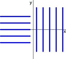
Figure 1: Orthogonal domain wall

Remark 15

Our method may be used for other physical problem displaying analogue patterns, such as, for example at a fluid-ferro-fluid interface, as studied in the symmetric case (”corner defect”) by J.Horn in [7]. More generally, any physical problem leading to a normal form such as (69) (see Appendix A.1) introduces the 4 important coefficients $(g,d_{2},d_{4},c_{9})$ of the cubic normal form, and should, after validation of the reduction, lead to a Theorem such as Theorem 8.

3 Setting of the perturbed system

3.1 Solutions at infinities

Since we leave now some freedom to the wave numbers, as well in the $y$ direction, as in the $x$ direction, the ”end points” of the expected heteroclinic are no longer $(1,0)$ at $-\infty,$ and the circle $(0,e^{i\phi})$ at $+\infty.$ In fact the classical study of steady convective rolls, shows that these should be respectively $(A_{0}^{(-\infty)}(k_{-}),B_{0}^{(-\infty)}(k_{-}))$ and $(0,B_{0}^{(+\infty)}(\omega,x))$ (see [4] section 4.3.3, or [5] sections 2 and 6.2). From Appendix A.2 for the equilibrium at $-\infty$, we have

$$(A_{0}^{(-\infty)})^{2} = 1-\frac{k_{-}^{2}}{4}+\mathcal{\sigma}_{0}\varepsilon^{2}k_{-}+\mathcal{O}(\varepsilon^{2}|k_{-}|^{3}+\varepsilon^{4}),$$

$$1-(A_{0}^{(-\infty)})\overset{def}{=}-\frac{\widetilde{\omega}_{-}^{2}}{2},\text{ with }\widetilde{\omega}_{-}^{2} = \frac{k_{-}^{2}}{4}-\mathcal{\sigma}_{0}\varepsilon^{2}k_{-}+\mathcal{O}[k_{-}^{4}+\varepsilon^{2}|k_{-}|^{3}+\varepsilon^{4}],$$

$$B_{0}^{(-\infty)} = \mathcal{O}(\varepsilon^{6}).$$

From Appendix A.3 for the periodic solutions at $+\infty,$ we have

$$e^{i\frac{x}{2\varepsilon}}B_{0}^{(+\infty)}(\omega,x) = r_{0}e^{i\omega x}+\mathcal{O}(\varepsilon^{6}),\text{ }A_{0}^{(+\infty)}=0,$$

$$\omega\overset{def}{=}\frac{1}{2\varepsilon}+\varepsilon\widetilde{\omega}_{+} = \frac{1+\varepsilon^{2}k_{+}}{2\varepsilon}+\mathcal{O}(\varepsilon^{7}),$$

$$B_{0}^{(+\infty)}e^{-i\varepsilon\widetilde{\omega}_{+}x}=C_{0}^{(+\infty)}+iD_{0}^{(+\infty)}$$

$$r_{0}^{2} = 1-\frac{k_{+}^{2}}{4}+\mathcal{O}(\varepsilon^{2}|k_{+}|+\varepsilon^{4})=1-\mathcal{O[}(\widetilde{|\omega}_{+}|+\varepsilon^{2})^{2}],$$

$$C_{0}^{(+\infty)} = r_{0}+\mathcal{O}(\varepsilon^{6}),\text{ oscil. part}(C_{0}^{(+\infty)})=\mathcal{O}(\varepsilon^{6}),$$

$$D_{0}^{(+\infty)} = \mathcal{O}(\varepsilon^{6}).$$

Remark 16

The coefficient $\sigma_{0}$ introduced in the expression of $(A_{0}^{(-\infty)})^{2}$ depends on the Prandtl number.

Remark 17

We may notice that in case the system has the symmetry $S_{0}$ representing $z\mapsto 1-z$ (OK for rigid-rigid, or free-free boundary conditions), then $B_{0}^{(-\infty)}=0,$ which simplifies computations (see Appendix A.2).

3.2 First change of variable

Let us set

$$B_{0}e^{-i\varepsilon\widetilde{\omega}_{+}x}=C_{0}+iD_{0},$$

then (3) becomes

$$A_{0}^{(4)}=k_{-}A_{0}^{\prime\prime}+A_{0}[1-\frac{k_{-}^{2}}{4}-A_{0}^{2}-g(C_{0}^{2}+D_{0}^{2})]+f$$ (7)

$$C_{0}^{\prime\prime} = 2\varepsilon\widetilde{\omega}_{+}D_{0}^{\prime}+\varepsilon^{2}C_{0}(-1+\widetilde{\omega}_{+}^{2}+gA_{0}^{2}+C_{0}^{2}+D_{0}^{2})+g_{r}$$ (8)

$$D_{0}^{\prime\prime} = -2\varepsilon\widetilde{\omega}_{+}C_{0}^{\prime}+\varepsilon^{2}D_{0}(-1+\widetilde{\omega}_{+}^{2}+gA_{0}^{2}+C_{0}^{2}+D_{0}^{2})+g_{i}$$

with

$$f=\widehat{f},\text{ \ }g_{r}+ig_{i}=\widehat{g}e^{-i\varepsilon\widetilde{\omega}_{+}x},$$

and where the exponential factor disappears in the cubic part when we replace $B_{0}$ by $(C_{0}+iD_{0})e^{i\varepsilon\widetilde{\omega}_{+}x}.$ Let us define

$$f = f_{0}(\varepsilon,k_{-},X,Y,\overline{Y})+f_{1}(\omega x,\varepsilon,k_{-},X,Y,\overline{Y})$$

$$g_{r} = g_{r0}(\varepsilon,X,Y,\overline{Y})+g_{r1}(\omega x,\varepsilon,k_{-},X,Y,\overline{Y})$$

$$g_{i} = g_{i0}(\varepsilon,X,Y,\overline{Y})+g_{i1}(\omega x,\varepsilon,k_{-},X,Y,\overline{Y}),$$

where $f_{0},g_{r0},g_{i0}$ come only from cubic terms of the normal form in (3), and where $f_{1},g_{r1},g_{i1}$ are $2\pi-$periodic in $\omega x$, smooth in their arguments, and satisfy estimates

$$|f_{1}(\omega x,\varepsilon,k_{-},X,Y,\overline{Y})| \leq c\varepsilon^{4}|X|(|X|^{2}+|Y|^{2})^{2}$$

$$|g_{r1}(\omega x,\varepsilon,k_{-},X,Y,\overline{Y})|+|g_{i1}(\omega x,\varepsilon,k_{-},X,Y,\overline{Y})| \leq c\varepsilon^{6}(|X|^{2}+|Y|)(|X|^{2}+|Y|^{2})^{2},$$

with

$$X = (A_{0},A_{0}^{\prime},A_{0}^{\prime\prime},A_{0}^{\prime\prime\prime})$$

$$Y = (C_{0}+iD_{0},C_{0}^{\prime}+iD_{0}^{\prime}).$$

Then we have from (4), (2):

$$f_{0} = d_{1}\varepsilon A_{0}(C_{0}D_{0}^{\prime}-D_{0}C_{0}^{\prime})+\sigma_{0}\varepsilon^{2}k_{-}A_{0}^{3}+d_{2}\varepsilon^{2}A_{0}A_{0}^{\prime 2}+d_{3}\varepsilon^{2}A_{0}^{\prime\prime}$$

$$+d_{4}\varepsilon^{2}A_{0}^{2}A_{0}^{\prime\prime}+d_{5}\varepsilon^{2}A_{0}^{\prime\prime}(C_{0}^{2}+D_{0}^{2})+d_{6}\varepsilon^{2}A_{0}(C_{0}^{\prime 2}+D_{0}^{\prime 2})+$$

$$+d_{7}\varepsilon^{2}A_{0}^{\prime}(C_{0}C_{0}^{\prime}+D_{0}D_{0}^{\prime})+d_{8}\varepsilon^{3}A_{0}^{\prime\prime}(C_{0}D_{0}^{\prime}-D_{0}C_{0}^{\prime})+\mathcal{O}(\varepsilon^{4}),$$

$$g_{r0}+ig_{i0} = i\varepsilon^{3}(C_{0}^{\prime}+iD_{0}^{\prime})[c_{0}+c_{1}A_{0}^{2}+c_{2}(C_{0}^{2}+D_{0}^{2})]$$

$$+\varepsilon^{3}c_{3}(C_{0}+iD_{0})(C_{0}D_{0}^{\prime}-D_{0}C_{0}^{\prime})+i\varepsilon^{3}c_{9}(C_{0}+iD_{0})A_{0}A_{0}^{\prime}$$

$$+\varepsilon^{4}c_{4}(C_{0}^{\prime}+iD_{0}^{\prime})(C_{0}D_{0}^{\prime}-D_{0}C_{0}^{\prime})+c_{5}\varepsilon^{4}A_{0}A_{0}^{\prime\prime}(C_{0}+iD_{0})$$

$$+\varepsilon^{4}[c_{6}A_{0}^{\prime 2}(C_{0}+iD_{0})+c_{7}A_{0}A_{0}^{\prime}(C_{0}^{\prime}+iD_{0}^{\prime})]$$

$$+i\varepsilon^{5}(C_{0}^{\prime}+iD_{0}^{\prime})(c_{7}A_{0}A_{0}^{\prime\prime}+c_{10}A_{0}^{\prime 2})$$

$$+i\varepsilon^{5}(C_{0}+iD_{0})(c_{8}A_{0}A_{0}^{\prime\prime\prime}+c_{11}A_{0}^{\prime}A_{0}^{\prime\prime})+\mathcal{O}(\varepsilon^{6}).$$

Now, let us set a first change of variables

$$A_{0} = A_{\ast}+\widetilde{A_{0}}$$

$$C_{0} = B_{\ast}+\widetilde{C_{0}}$$ (11)

$$D_{0} = \widetilde{D_{0}}$$

where we observe that we expect

$$\widetilde{A_{0}}\underset{x=-\infty}{\rightarrow}A_{0}^{(-\infty)}-1 = -\frac{\widetilde{\omega}_{-}^{2}}{2},\text{ }$$

$$C_{0}+iD_{0}\underset{x=-\infty}{\rightarrow}C_{0}^{(-\infty)} = B_{0}^{(-\infty)}=\mathcal{O}(\varepsilon^{6}),$$

$$\widetilde{C_{0}}+i\widetilde{D_{0}}\underset{x=+\infty}{\rightarrow}C_{0}^{(+\infty)}+iD_{0}^{(+\infty)}-1 \sim -\frac{(\widetilde{\omega}_{+}+\mathcal{O}(\varepsilon^{2}))^{2}}{2}.$$

Then (7,8) becomes the ”perturbed system”

$$\mathcal{M}_{g}(\widetilde{A_{0}},\widetilde{C_{0}})=\binom{-k_{-}(A_{\ast}^{\prime\prime}+\widetilde{A_{0}}^{\prime\prime})+\frac{k_{-}^{2}}{4}(A_{\ast}+\widetilde{A_{0}})+\widetilde{\phi_{0}}}{\frac{2\widetilde{\omega}_{+}}{\varepsilon}\widetilde{D_{0}}^{\prime}+\widetilde{\omega}_{+}^{2}(B_{\ast}+\widetilde{C_{0}})+\widetilde{\psi_{0r}}},$$ (12)

$$\mathcal{L}_{g}\widetilde{D_{0}}=-\frac{2\widetilde{\omega}_{+}}{\varepsilon}(B_{\ast}^{\prime}+\widetilde{C_{0}}^{\prime})+\widetilde{\omega}_{+}^{2}\widetilde{D_{0}}+\widetilde{\psi_{0i}},$$ (13)

where linear operators $\mathcal{M}_{g}$ and $\mathcal{L}_{g}$ are defined as

$$\mathcal{M}_{g}\left(\begin{array}[]{c}A\\ C\end{array}\right)=\left(\begin{array}[]{c}-A^{(4)}+(1-3A_{\ast}^{2}-gB_{\ast}^{2})A-2gA_{\ast}B_{\ast}C\\ \frac{1}{\varepsilon^{2}}C^{\prime\prime}+(1-gA_{\ast}^{2}-3B_{\ast}^{2})C-2gA_{\ast}B_{\ast}A\end{array}\right),$$ (14)

$$\mathcal{L}_{g}D=\frac{1}{\varepsilon^{2}}D^{\prime\prime}+(1-gA_{\ast}^{2}-B_{\ast}^{2})D,$$ (15)

and where $\widetilde{\phi_{0}},\widetilde{\psi_{0r}},\widetilde{\psi_{0i}}$ are smooth functions of $(\omega x,\varepsilon,k_{-},\widetilde{\omega}_{+},\widetilde{X},\widetilde{Y})$ where

$$\widetilde{X} = (\widetilde{A_{0}},\widetilde{A_{0}}^{\prime},\widetilde{A_{0}}^{\prime\prime},\widetilde{A_{0}}^{\prime\prime\prime})$$

$$\widetilde{Y} = (\widetilde{C_{0}},\widetilde{D_{0}},\widetilde{C_{0}}^{\prime},\widetilde{D_{0}}^{\prime})$$

$$\widetilde{\phi_{0}} = \widetilde{\phi_{00}}(\varepsilon,k_{-},\widetilde{X},\widetilde{Y})+\widetilde{\phi_{01}}(\omega x,\varepsilon,k_{-},\widetilde{X},\widetilde{Y})$$

$$\widetilde{\psi_{0r}} = \widetilde{\psi_{0r0}}(\varepsilon,k_{-},\widetilde{X},\widetilde{Y})+\widetilde{\psi_{0r1}}(\omega x,\varepsilon,k_{-},\widetilde{X},\widetilde{Y})$$

$$\widetilde{\psi_{0i}} = \widetilde{\psi_{0i0}}(\varepsilon,k_{-},\widetilde{X},\widetilde{Y})+\widetilde{\psi_{0i1}}(\omega x,\varepsilon,k_{-},\widetilde{X},\widetilde{Y})$$

$$|\widetilde{\phi_{01}}(\omega x,\varepsilon,k_{-},\widetilde{X},\widetilde{Y})| \leq c\varepsilon^{4}$$ (16)

$$|\widetilde{\psi_{0r1}}(\omega x,\varepsilon,k_{-},\widetilde{X},\widetilde{Y})|+|\widetilde{\psi_{0i1}}(\omega x,\varepsilon,k_{-},\widetilde{X},\widetilde{Y})| \leq c\varepsilon^{4}.$$

More precisely, we have

$$\widetilde{\phi_{00}}(\varepsilon,k_{-},\widetilde{X},\widetilde{Y}) = 3A_{\ast}\widetilde{A_{0}}^{2}+\widetilde{A_{0}}^{3}+2gB_{\ast}\widetilde{A_{0}}\widetilde{C_{0}}$$

$$+g(A_{\ast}+\widetilde{A_{0}})(\widetilde{C_{0}}^{2}+\widetilde{D_{0}}^{2})+f_{00},$$

$$\widetilde{\psi_{0r0}}(\varepsilon,k_{-},\widetilde{X},\widetilde{Y}) = 2gA_{\ast}\widetilde{A_{0}}\widetilde{C_{0}}+gB_{\ast}\widetilde{A_{0}}^{2}+2B_{\ast}\widetilde{C_{0}}^{2}+g\widetilde{A_{0}}^{2}\widetilde{C_{0}}$$

$$+(B_{\ast}+\widetilde{C_{0}})(\widetilde{C_{0}}^{2}+\widetilde{D_{0}}^{2})+g_{00r},$$

$$\widetilde{\psi_{0i0}}(\varepsilon,k_{-},\widetilde{X},\widetilde{Y}) = 2gA_{\ast}\widetilde{A_{0}}\widetilde{D_{0}}+2B_{\ast}\widetilde{C_{0}}\widetilde{D_{0}}+g\widetilde{A_{0}}^{2}\widetilde{D_{0}}$$ (19)

$$+\widetilde{D_{0}}(\widetilde{C_{0}}^{2}+\widetilde{D_{0}}^{2})+g_{00i},$$

and in using Theorem 5, Corollaries 6 and 7, and assuming

$$|\widetilde{X}|\leq 1,|\widetilde{Y}|\leq 1,|\widetilde{D_{0}}|\leq\varepsilon,$$ (20)

$$f_{00} = \sigma_{0}\varepsilon^{2}k_{-}A_{\ast}^{3}+\mathcal{O}[\varepsilon^{2+3/5}e^{\varepsilon\delta_{\ast}x}\chi_{(-\infty,0)}+\varepsilon^{2+2/5}e^{-\varepsilon^{1/5}\delta_{\ast}x}\chi_{(0,\infty)}+\varepsilon^{2}(|\widetilde{X}|+|\widetilde{Y}|)+\varepsilon|\widetilde{D_{0}}^{\prime}|],$$

$$g_{00r} = \mathcal{O}[\varepsilon^{2+3/5}e^{\varepsilon\delta_{\ast}x}\chi_{(-\infty,0)}+\varepsilon^{2+4/5}e^{-\varepsilon^{1/5}\delta_{\ast}x}\chi_{(0,\infty)}+\varepsilon^{2}(|\widetilde{X}|+|\widetilde{Y}|)+\varepsilon|\widetilde{D_{0}}^{\prime}|],$$

$$g_{00i} = \mathcal{O}[\varepsilon^{1+3/5}e^{\varepsilon\delta_{\ast}x}\chi_{(-\infty,0)}+\varepsilon^{1+4/5}e^{-\varepsilon^{1/5}\delta_{\ast}x}\chi_{(0,\infty)}+\varepsilon(|\widetilde{X}|+|\widetilde{Y}|)+\varepsilon(|\widetilde{C_{0}}^{\prime}|],$$

where $f_{00}$ and $g_{00r}+ig_{00i}$ are smooth functions which come from the rest of the cubic normal form written in (3.2,3.2)) and $\chi_{(-\infty,0)}$ and $\chi_{(0,\infty)}$ are the characteristic functions on the corresponding intervals.

Remark 18

We notice that the estimates for the main terms independent of $\widetilde{X},\widetilde{Y}$ come from

$$\text{for }f_{00} : \text{ }\sigma_{0}\varepsilon^{2}k_{-}A_{\ast}^{3}+d_{2}\varepsilon^{2}A_{\ast}A_{\ast}^{\prime 2}+d_{3}\varepsilon^{2}A_{\ast}^{\prime\prime}+d_{4}\varepsilon^{2}A_{\ast}^{2}A_{\ast}^{\prime\prime}+d_{5}\varepsilon^{2}A_{\ast}^{\prime\prime}B_{\ast}^{2},$$

$$\text{for }g_{00r} : \text{ }c_{5}\varepsilon^{2}A_{\ast}A_{\ast}^{\prime\prime}B_{\ast}+c_{6}\varepsilon^{2}A_{\ast}^{\prime 2}B_{\ast}+c_{7}\varepsilon^{2}A_{\ast}A_{\ast}^{\prime}B_{\ast}^{\prime}$$

$$\text{for }g_{00i} : \text{ }\varepsilon B_{\ast}^{\prime}(c_{0}+c_{1}A_{\ast}^{2}+c_{2}B_{\ast}^{2})+\varepsilon c_{9}B_{\ast}A_{\ast}A_{\ast}^{\prime}.$$

Moreover, notice that, below, we need to compute $\int f_{00}A_{\ast}^{\prime}dx,$ $\int g_{00r}B_{\ast}^{\prime}dx,$ $\int g_{00i}B_{\ast}dx,$ which, for terms independent of $\widetilde{X},\widetilde{Y}$ leads to

$$\text{for }\int f_{00}A_{\ast}^{\prime}dx = -\frac{\sigma_{0}\varepsilon^{2}k_{-}}{4}+\varepsilon^{2}\int(d_{2}A_{\ast}A_{\ast}^{\prime 3}+d_{4}A_{\ast}^{2}A_{\ast}^{\prime}A_{\ast}^{\prime\prime})dx+\mathcal{O}(\varepsilon^{3})$$

$$= -\frac{\sigma_{0}\varepsilon^{2}k_{-}}{4}+\mathcal{O}(\varepsilon^{2+4/5}),$$

$$\text{for }\int g_{00r}B_{\ast}^{\prime}dx \sim \varepsilon^{2}\int_{\mathbb{R}}c_{5}A_{\ast}A_{\ast}^{\prime\prime}B_{\ast}B_{\ast}^{\prime}dx+\varepsilon^{2}\int_{\mathbb{R}}c_{6}A_{\ast}^{\prime 2}B_{\ast}B_{\ast}^{\prime}dx=\mathcal{O}(\varepsilon^{3+1/5}),$$

$$\text{for }\int g_{00i}B_{\ast}dx = \varepsilon(\frac{c_{0}}{2}+\frac{c_{2}}{4})+\varepsilon(c_{1}-c_{9})\int_{\mathbb{R}}A_{\ast}^{2}B_{\ast}B_{\ast}^{\prime}=\mathcal{O}(\varepsilon),$$

where we notice

$$\int A_{\ast}^{\prime\prime}A_{\ast}^{\prime}dx = 0,\text{ }\varepsilon^{2}\int A_{\ast}^{\prime\prime}B_{\ast}^{2}A_{\ast}^{\prime}dx=-\varepsilon^{2}\int A_{\ast}^{\prime 2}B_{\ast}B_{\ast}^{\prime}dx=\mathcal{O}(\varepsilon^{3}),$$

$$\int(d_{2}A_{\ast}A_{\ast}^{\prime 3}+d_{4}A_{\ast}^{2}A_{\ast}^{\prime}A_{\ast}^{\prime\prime})dx = (d_{2}-d_{4})\int A_{\ast}A_{\ast}^{\prime 3}dx=\mathcal{O}(\varepsilon^{1/2}),$$

$$\int_{\mathbb{R}}A_{\ast}A_{\ast}^{\prime\prime}B_{\ast}B_{\ast}^{\prime}dx = -\int_{\mathbb{R}}[A_{\ast}^{\prime 2}B_{\ast}B_{\ast}^{\prime}+A_{\ast}A_{\ast}^{\prime}(B_{\ast}B_{\ast}^{\prime})^{\prime}]dx,$$

taking care of the convergence in $e^{\varepsilon\delta_{\ast}x}$ (resp $e^{-\varepsilon^{1/5}\delta_{\ast}x})$ at $-\infty$ (resp at $+\infty),$ which implies a division by $\varepsilon$ in the integral on $(-\infty,0)$ (resp. by $\varepsilon^{1/5}$ in the integral on $(0,+\infty)).$

3.3 Second change of variables

Before solving the system we need to change variables so that the variables and the right hand side of (12,13) tend towards $0$ at infinity. Let us denote

$$\widetilde{X}^{(-\infty)} = (A_{0}^{(-\infty)}-1,0,0,0)=(\mathcal{O}(\widetilde{\omega}_{-}^{2}),0,0,0)$$

$$\widetilde{Y}^{(-\infty)} = (C_{0}^{(-\infty)},0,0,0)=(\mathcal{O}(\varepsilon^{6}),0,0,0),$$

$$\widetilde{X}^{(+\infty)} = 0$$

$$\widetilde{Y}^{(+\infty)} = (C_{0}^{(+\infty)}-1,D_{0}^{(+\infty)},C_{0}^{(+\infty)\prime},D_{0}^{(+\infty)\prime})=[\mathcal{O}((\widetilde{\omega}_{+}+\varepsilon^{2})^{2}),\mathcal{O}(\varepsilon^{6}),\mathcal{O}(\varepsilon^{5}),\mathcal{O}(\varepsilon^{5})],$$

then, taking care in (7,8), of the forms of $f$, $g_{r},$ $g_{i},$ we notice that the limit terms in the right hand side of (12,13) as $x\rightarrow-\infty$ are

$$\frac{k_{-}^{2}}{4}A_{0}^{(-\infty)}+\widetilde{\phi_{0}}(\omega x,\varepsilon,k_{-},\widetilde{X}^{(-\infty)},\widetilde{Y}^{(-\infty)})\text{ exp limit as }e^{\varepsilon\delta_{\ast}x}\text{ (see }f_{00}),$$

$$\widetilde{\omega}_{+}^{2}C_{0}^{(-\infty)}+\widetilde{\psi_{0r}}(\omega x,\varepsilon,k_{-},\widetilde{X}^{(-\infty)},\widetilde{Y}^{(-\infty)})\text{ exp limit as }e^{\varepsilon\delta_{\ast}x}\text{ (see }g_{00r})$$

$$\widetilde{\psi_{0i}}(\omega x,\varepsilon,k_{-},\widetilde{X}^{(-\infty)},\widetilde{Y}^{(-\infty)})\text{ exp limit as }e^{\varepsilon\delta_{\ast}x}\text{ (as }B_{\ast}^{\prime}\text{ and see }g_{00i}).$$

The limit terms of the right hand side of (12,13) as $x\rightarrow+\infty$ is

$$0\text{ exp limit as }e^{-\varepsilon^{1/5}\delta_{\ast}x}\text{ (as }A_{\ast})$$

$$\frac{2\widetilde{\omega}_{+}}{\varepsilon}(D_{0}^{(+\infty)})^{\prime}+\widetilde{\omega}_{+}^{2}C_{0}^{(+\infty)}+\widetilde{\psi_{0r}}(\omega x,\varepsilon,k_{-},0,\widetilde{Y}^{(+\infty)})\text{ exp limit as }e^{-\varepsilon^{1/5}\delta_{\ast}x}\text{ (see }g_{00r}),$$

$$-\frac{2\widetilde{\omega}_{+}}{\varepsilon}(C_{0}^{(+\infty)})^{\prime}+\widetilde{\omega}_{+}^{2}D_{0}^{(+\infty)}+\widetilde{\psi_{0i}}(\omega x,\varepsilon,k_{-},0,\widetilde{Y}^{(+\infty)})\text{ exp limit as }e^{-\varepsilon\sqrt{2}x}\text{ (see }g_{00i}).$$

Let us make a second change of variables as

$$\widetilde{A_{0}} = \alpha_{-}\chi_{-}+\widehat{A_{0}}$$

$$\widetilde{C_{0}} = \beta_{-}\chi_{-}+\beta_{+}\chi_{+}+\widehat{C_{0}},$$ (21)

$$\widetilde{D_{0}} = \gamma_{+}\chi_{+}+\widehat{D_{0}},$$

with (in using Appendix A.2 and (77) in Appendix A.3)

$$\alpha_{-} = (A_{0}^{(-\infty)}-1)=\mathcal{-}\widetilde{\omega}_{-}^{2}/2,\text{ }\beta_{-}=B_{0}^{(-\infty)},$$ (22)

$$\beta_{+} = (C_{0}^{(+\infty)}(\omega x)-1),\text{ }\gamma_{+}=D_{0}^{(+\infty)}(\omega x),$$

$$\text{const part of }\beta_{+}\overset{def}{=}\beta_{+}^{(c)}=-\frac{\widetilde{\omega}_{+}^{2}}{2}+\frac{\sigma_{1}\varepsilon^{2}\widetilde{\omega}_{+}}{2}+\frac{\sigma_{2}\varepsilon^{4}}{2}+\mathcal{O[}(|\widetilde{\omega}_{+}|+\varepsilon^{2})^{4}],$$ (23)

and where $\chi_{-}$ and $\chi_{+}$ are smooth functions, such that

$$\chi_{-} = 1\text{ for }x\in(-\infty,-1),$$

$$= 0\text{ for }x>0$$

$$0 < \chi_{-}<1\text{ for }x\in(-1,0),$$

$$\chi_{+} = 1\text{ for }x\in(1,\infty),$$

$$= 0\text{ for }x<0$$

$$0 < \chi_{+}<1\text{ for }x\in(0,1),$$

such that

$$(\widehat{A_{0}},\widehat{C_{0}},\widehat{D_{0}})\rightarrow 0\text{ as }|x|\rightarrow\infty.$$

3.4 Properties of linear operators $\mathcal{M}_{g}$ and $\mathcal{L}_{g}$ (defined in (14,15))

We now give a precise definition of the function spaces where we will solve the problem with respect to $(\widehat{A_{0}},\widehat{C_{0}},\widehat{D_{0}}).$ Indeed, let us define the Hilbert spaces

$$L_{\eta}^{2}=\{u;u(x)e^{\eta|x|}\in L^{2}(\mathbb{R})\},$$

$$\mathcal{D}_{0} = \{(A,C)\in H_{\eta}^{4}\times H_{\eta}^{2};A\in H_{\eta}^{4},C\in\mathcal{D}_{1}\}$$

$$\mathcal{D}_{1} = \{C\in H_{\eta}^{2};\varepsilon^{-2}||C^{\prime\prime}||_{L_{\eta}^{2}}+\varepsilon^{-1}||C^{\prime}||_{L_{\eta}^{2}}+||C||_{L_{\eta}^{2}}\overset{def}{=}||C||_{\mathcal{D}_{1}}<\infty\}$$

equiped with natural scalar products. Then we have the following result (proved in [10]):

Lemma 19

Except maybe for a set of isolated values of $g,$ the kernel of $\mathcal{M}_{g}$ in $L_{\eta}^{2}$ is one dimensional, spanned by $(A_{\ast}^{\prime},B_{\ast}^{\prime}),$ and its range has codimension 1, $L^{2}$- orthogonal to $(A_{\ast}^{\prime},B_{\ast}^{\prime}).$ $\mathcal{M}_{g}$ has a pseudo-inverse acting from $L_{\eta}^{2}$ to $\mathcal{D}_{0}$ for any $\eta>0$ small enough, with bound independent of $\varepsilon.$

The operator $\mathcal{L}_{g}$ has a trivial kernel, and its range which has codimension 1, is $L^{2}$- orthogonal to $B_{\ast}$ ($B_{\ast}\notin L^{2}).$ $\mathcal{L}_{g}$ has a pseudo-inverse acting respectively from $L_{\eta}^{2}$ to $\mathcal{D}_{1}$ for $\eta>0$ small enough, with bound independent of $\varepsilon.$

Remark 20

We might expect a two-dimensional kernel since we have a ”circle” of heteroclinics. The one-dimensional kernel of $\mathcal{M}_{g}$ is the usual one, while we also have $\mathcal{L}_{g}B_{\ast}=0.$ However $B_{\ast}\notin L_{\eta}^{2}$ so that the kernel of $\mathcal{L}_{g}$ is $\{0\},$ and we pay this by a codimension one range for $\mathcal{L}_{g}.$ This is explicitely computed in [10].

4 Estimates for the right hand sides of $\mathcal{M}_{g}(\widehat{A_{0}},\widehat{C_{0}})$ and $\mathcal{L}_{g}\widehat{D_{0}}$

After the second change of variables (21) the remaining terms in the right hand side of $\mathcal{M}_{g}(\widehat{A_{0}},\widehat{C_{0}})$ and $\mathcal{L}_{g}\widehat{D_{0}}$ coming from

$$\widetilde{\phi_{01}}(\omega x,\varepsilon,k_{-},\widetilde{X},\widetilde{Y}),\text{ }\widetilde{\psi_{0r1}}(\omega x,\varepsilon,k_{-},\widetilde{X},\widetilde{Y}),\text{ }\widetilde{\psi_{0i1}}(\omega x,\varepsilon,k_{-},\widetilde{X},\widetilde{Y})$$

now cancel for $(\widehat{X},\widehat{Y},\widehat{\overline{Y}})=0,$ they are then estimated in $L_{\eta}^{2}$ by

$$\mathcal{O}(\varepsilon^{4}(||(\widehat{A_{0}},\widehat{C_{0}})||_{\mathcal{D}_{0}}+||\widehat{D_{0}}||_{\mathcal{D}_{1}}),$$ (24)

provided that the following condition

$$|\widehat{A_{0}}(x)|+|\widehat{A_{0}^{\prime}}(x)|+|\widehat{A_{0}^{\prime\prime}}(x)|+|\widehat{A_{0}^{\prime\prime\prime}}(x)|+|\widehat{C_{0}}(x)|+|\widehat{C_{0}^{\prime}}(x)|+|\widehat{D_{0}}(x)|+|\widehat{D_{0}^{\prime}}(x)|<<1$$ (25)

holds. We need to check this condition at the end of subsection 5.3. The unknowns in the problem are now

$$(\widehat{A_{0}},\widehat{C_{0}})\in\mathcal{D}_{0},\text{ }\widehat{D_{0}}\in\mathcal{D}_{1},\text{ }(k_{-},\widetilde{\omega}_{+})\in\mathbb{R}^{2},$$

and $\varepsilon$ is supposed to be small enough. In the following we use extensively the estimates (see (22,23))

$$\alpha_{-} = \mathcal{O}(|k_{-}|+\varepsilon^{2})^{2},\text{ \ }\beta_{+}=\mathcal{O}(|\widetilde{\omega}_{+}|+\varepsilon^{2})^{2},$$

$$\beta_{-} = \mathcal{O}(\varepsilon^{6}),\text{ oscil part }(\beta_{+})=\mathcal{O}(\varepsilon^{6}),\text{ }\gamma_{+}=\mathcal{O}(\varepsilon^{6}),$$

$$\beta_{+}^{\prime} = \mathcal{O}(\varepsilon^{5}),\text{ }\gamma_{+}^{\prime}=\mathcal{O}(\varepsilon^{5}).$$

4.1 First component of $\mathcal{M}_{g}(\widehat{A_{0}},\widehat{C_{0}})$

The first component is now the sum of small terms linear in $(\widehat{A_{0}},\widehat{C_{0}})$ plus quadratic terms and terms independent of $(\widehat{A_{0}},\widehat{C_{0}})$ which tend exponentially to $0$ as $e^{\varepsilon\delta_{\ast}x}$ for $x\rightarrow-\infty$ and $e^{-\sqrt{2}\varepsilon x}$ for $x\rightarrow+\infty:$

$$\mathcal{M}_{g}(\widehat{A_{0}},\widehat{C_{0}})|_{1}=-k_{-}\widehat{A_{0}}^{\prime\prime}+\frac{k_{-}^{2}}{4}\widehat{A_{0}}+\widehat{\phi_{0}}+\varphi_{1}(k_{-})$$ (26)

with

$$\varphi_{1}(k_{-}) = -k_{-}(A_{\ast}^{\prime\prime}+\alpha_{-}\chi_{-}^{\prime\prime})+\frac{k_{-}^{2}}{4}(A_{\ast}-\chi_{-})+\alpha_{-}\chi_{-}^{(4)}$$

$$-3(1-A_{\ast}^{2})\alpha_{-}\chi_{-}+gB_{\ast}^{2}\alpha_{-}\chi_{-}+2gA_{\ast}B_{\ast}(\beta_{-}\chi_{-}+\beta_{+}\chi_{+}),$$

$$\widehat{\phi_{0}} = \widetilde{\phi_{0}}(\omega x,\varepsilon,k_{-},\widetilde{X},\widetilde{Y})-\chi_{-}\widetilde{\phi_{0}}(\omega x,\varepsilon,k_{-},\widetilde{X}^{(-\infty)},\widetilde{Y}^{(-\infty)}).$$

More precisely we have, from (3.2), and taking into account (24)

$$\widehat{\phi_{0}} = 3[\alpha_{-}^{2}(A_{\ast}\chi_{-}^{2}-\chi_{-})+2\alpha_{-}A_{\ast}\chi_{-}\widehat{A_{0}}+A_{\ast}\widehat{A_{0}}^{2}]+\alpha_{-}^{3}(\chi_{-}^{3}-\chi_{-})$$

$$+3\alpha_{-}^{2}\chi_{-}^{2}\widehat{A_{0}}+3\alpha_{-}\chi_{-}\widehat{A_{0}}^{2}+\widehat{A_{0}}^{3}+2gB_{\ast}[\alpha_{-}\chi_{-}\widehat{C_{0}}+(\beta_{-}\chi_{-}+\beta_{+}\chi_{+})\widehat{A_{0}}+\widehat{A_{0}}\widehat{C_{0}}]$$

$$+g(A_{\ast}+\alpha_{-}\chi_{-}+\widehat{A_{0}})[(\beta_{-}\chi_{-}+\beta_{+}\chi_{+}+\widehat{C_{0}})^{2}+(\gamma_{+}\chi_{+}+\widehat{D_{0}})^{2}]$$

$$-\chi_{-}g(1+\alpha_{-})\beta_{-}^{2}+\widehat{f_{00}},$$

$$\widehat{f_{00}} = \sigma_{0}\varepsilon^{2}k_{-}(A_{\ast}^{3}-\chi_{-})+\mathcal{O}[\varepsilon^{2+2/5}(e^{\varepsilon\delta_{\ast}x}\chi_{(-\infty,0)}+e^{-\varepsilon^{1/5}\delta_{\ast}x}\chi_{(0,\infty)})+\varepsilon^{2}(|\widehat{X}|+|\widehat{Y}|)+\varepsilon|\widehat{D_{0}}^{\prime}|].$$

We notice that for $\eta=\varepsilon\delta_{\ast}/2$ $(\eta<\varepsilon\delta$ is necessary$),$ and due to Corollary 7,

$$\frac{1}{\varepsilon^{2}}\beta_{+}^{\prime} = \mathcal{O}(\varepsilon^{3}),\text{ }\frac{1}{\varepsilon^{2}}\gamma_{+}^{\prime}=\mathcal{O}(\varepsilon^{3}),$$

$$||A_{\ast}^{\prime}||_{L_{\eta}^{2}} = \mathcal{O}(\varepsilon^{1/10}),\text{ }||B_{\ast}^{\prime}||_{L_{\eta}^{2}}=\mathcal{O}(\varepsilon^{1/2}),$$

$$||A_{\ast}^{\prime 2}||_{L_{\eta}^{2}} = \mathcal{O}(\varepsilon^{7/10}),\text{ }||B_{\ast}^{\prime 2}||_{L_{\eta}^{2}}=\mathcal{O}(\varepsilon^{3/2}),$$

$$||A_{\ast}^{\prime\prime}||_{L_{\eta}^{2}} = \mathcal{O}(\varepsilon^{1/10}),\text{ }||B_{\ast}^{\prime\prime}||_{L_{\eta}^{2}}=\mathcal{O}(\varepsilon^{3/2}).$$

Then, in using extensively $2|ab|\leq a^{2}+b^{2})$ and, for example

$$\frac{k_{-}^{2}}{4}||A_{\ast}-\chi_{-}||_{L_{\eta}^{2}}=\mathcal{O(}\frac{k_{-}^{2}}{\sqrt{\varepsilon}}),$$

we obtain the estimates (here and in the following $c$ is a generic constant, independent of $\varepsilon)$

$$||\varphi_{1}(k_{-})||_{L_{\eta}^{2}} \leq c\left(\varepsilon^{1/10}|k_{-}|+\frac{k_{-}^{2}+\varepsilon^{4}}{\sqrt{\varepsilon}}+\widetilde{\omega}_{+}^{2}+\varepsilon^{2}|\widetilde{\omega}_{+}|)\right),$$ (29)

$$\int_{\mathbb{R}}\varphi_{1}(k_{-})A_{\ast}^{\prime}dx = \mathcal{O}[(|k_{-}|+|\widetilde{\omega}_{+}|+\varepsilon^{2})^{2}],$$

using integration by parts and

$$\int_{\mathbb{R}}A_{\ast}^{\prime}A_{\ast}^{\prime\prime}dx = 0,$$

$$\int_{\mathbb{R}}(A_{\ast}-\chi_{-})A_{\ast}^{\prime}dx = \mathcal{O}(1)$$

$$\int_{\mathbb{R}}(1-A_{\ast}^{2})A_{\ast}^{\prime}\chi_{-}dx = \mathcal{O}(1).$$

In next estimates, we use the following little Lemma (adapted from a simple Sobolev inequality) where we notice that we loose one $\varepsilon,$ due to the weak exponential decay at $\infty:$

Lemma 21

For any $u\in H_{\eta}^{1}$ and $\varepsilon$ sufficiently small, we have

$$|u(x)|\leq c(||u||_{L_{\eta}^{2}}+\frac{1}{\varepsilon}||u^{\prime}||_{L_{\eta}^{2}})$$

where $c$ is independent of $\varepsilon.$

Then we may use

$$|\widehat{A_{0}}^{(m)}(x)| \leq \frac{c}{\varepsilon}||\widehat{A_{0}}||_{H_{\eta}^{4}},\text{ }m=0,1,2,3$$

$$|\widehat{C_{0}}^{(m)}(x)| \leq c\varepsilon^{m}||\widehat{C_{0}}||_{\mathcal{D}_{1}},\text{ }m=0,1,$$

$$|\widehat{D_{0}}^{(m)}(x)| \leq c\varepsilon^{m}||\widehat{D_{0}}||_{\mathcal{D}_{1}},\text{ }m=0,1.$$

Now, from $f_{00}$ in (4.1), we have (see Remark 18)

$$||d_{3}\varepsilon^{2}A_{\ast}^{\prime\prime}+d_{4}\varepsilon^{2}A_{\ast}^{2}A_{\ast}^{\prime\prime}+d_{5}\varepsilon^{2}A_{\ast}^{\prime\prime}B_{\ast}^{2}||_{L_{\eta}^{2}}=\mathcal{O}(\varepsilon^{2+1/10}),$$

and for example, from Lemma 21

$$2g||B_{\ast}\widehat{A_{0}}\widehat{C_{0}}||_{L_{\eta}^{2}}\leq c||\widehat{A_{0}}||_{H_{\eta}^{4}}||\widehat{C_{0}}||_{\mathcal{D}_{1}}\leq c||(\widehat{A_{0}},\widehat{C_{0}})||_{\mathcal{D}_{0}}^{2},$$

$$||\widehat{A_{0}}^{2}||_{L_{\eta}^{2}}\leq\frac{c}{\varepsilon}||\widehat{A_{0}}||_{\mathcal{D}_{0}}^{2},\text{ \ }||\widehat{A_{0}}^{3}||_{L_{\eta}^{2}}\leq\frac{c}{\varepsilon^{2}}||\widehat{A_{0}}||_{\mathcal{D}_{0}}^{3}.$$

We then obtain, for sufficiently small $\varepsilon,|k_{-}|,|\widetilde{\omega}_{+}|,\widehat{A_{0}},\widehat{C_{0}},\widehat{D_{0}}$ in $\mathbb{R}_{+}^{3}\times\mathcal{D}_{0}\times\mathcal{D}_{1}$

$$||\widehat{\phi_{0}}||_{L_{\eta}^{2}}\leq c\left(\varepsilon^{2+1/10}+\varepsilon^{3/2}|k_{-}|+\frac{k_{-}^{4}}{\sqrt{\varepsilon}}+\widetilde{\omega}_{+}^{4}+\frac{1}{\varepsilon}||\widehat{A_{0}}||_{H_{\eta}^{4}}^{2}+\frac{1}{\varepsilon^{2}}||\widehat{A_{0}}||_{H_{\eta}^{4}}^{3}+||\widehat{C_{0}}||_{\mathcal{D}_{1}}^{2}+||\widehat{D_{0}}||_{\mathcal{D}_{1}}^{2}\right).$$ (30)

4.2 Second component of $\mathcal{M}_{g}(\widehat{A_{0}},\widehat{C_{0}})$

For the second component we have

$$\mathcal{M}_{g}(\widehat{A_{0}},\widehat{C_{0}})|_{2}=\frac{2\widetilde{\omega}_{+}}{\varepsilon}\widehat{D_{0}}^{\prime}+\widetilde{\omega}_{+}^{2}\widehat{C_{0}}+\widehat{\psi_{0r}}+\varphi_{2}(k_{-}),$$ (31)

with

$$\varphi_{2}(k_{-}) = \widetilde{\omega}_{+}^{2}(B_{\ast}-\chi_{+})-\frac{1}{\varepsilon^{2}}\beta_{-}\chi_{-}^{\prime\prime}-\frac{2}{\varepsilon^{2}}\beta_{+}^{\prime}\chi_{+}^{\prime}-\frac{1}{\varepsilon^{2}}\beta_{+}\chi_{+}^{\prime\prime}+\frac{2\widetilde{\omega}_{+}}{\varepsilon}\gamma_{+}\chi_{+}^{\prime}$$

$$-(3-gA_{\ast}^{2}-3B_{\ast}^{2})\beta_{+}\chi_{+}+[1-\chi_{-}-g(A_{\ast}^{2}-\chi_{-})]\beta_{-}\chi_{-}+2gA_{\ast}B_{\ast}\alpha_{-}\chi_{-},$$

$$\widehat{\psi_{0r}} = \widetilde{\psi_{0r}}(\omega x,\varepsilon,k_{-},\widetilde{X},\widetilde{Y})-\chi_{+}\widetilde{\psi_{0r}}(\omega x,\varepsilon,k_{-},0,\widetilde{Y}^{(+\infty)})$$

$$-\chi_{-}\widetilde{\psi_{0r}}(\omega x,\varepsilon,k_{-},\widetilde{X}^{(-\infty)},\widetilde{Y}^{(-\infty)}),$$

where $\gamma_{+}=D_{0}^{(+\infty)}.$ For $\widehat{\psi_{0r}}$ we have

$$\widehat{\psi_{0r}} = 2gA_{\ast}(\alpha_{-}\chi_{-}\widehat{C_{0}}+(\beta_{-}\chi_{-}+\beta_{+}\chi_{+})\widehat{A_{0}}+\widehat{A_{0}}\widehat{C_{0}})$$

$$+g(B_{\ast}+\beta_{+}\chi_{+}+\widehat{C_{0}})(\alpha_{-}^{2}\chi_{-}^{2}+2\alpha_{-}\chi_{-}\widehat{A_{0}}+\widehat{A_{0}}^{2})$$

$$+g\beta_{-}\chi_{-}[(\alpha_{-}^{2}(\chi_{-}^{2}-1)+2\alpha_{-}\chi_{-}\widehat{A_{0}}+\widehat{A_{0}}^{2}]$$

$$+[B_{\ast}(\beta_{-}\chi_{-}+\beta_{+}\chi_{+})^{2}-\chi_{+}\beta_{+}^{2}]+[B_{\ast}(\gamma_{+}\chi_{+})^{2}-\chi_{+}\gamma_{+}^{2}]$$

$$+\beta_{+}\chi_{+}(\chi_{+}^{2}-1)(\beta_{+}^{2}+\gamma_{+}^{2})+\beta_{-}^{3}\chi_{-}(\chi_{-}^{2}-1)$$

$$+\widehat{C_{0}}[(\beta_{-}\chi_{-}+\beta_{+}\chi_{+}+\widehat{C_{0}})^{2}+(\gamma_{+}\chi_{+}+\widehat{D_{0}})^{2}]$$

$$+2(B_{\ast}+\beta_{+}\chi_{+})(\beta_{-}\chi_{-}+\beta_{+}\chi_{+}\widehat{C_{0}}+\gamma_{+}\chi_{+}\widehat{D_{0}})$$

$$+(B_{\ast}+\beta_{-}\chi_{-}+\beta_{+}\chi_{+})(\widehat{C_{0}}^{2}+\widehat{D_{0}}^{2})+\widehat{g_{00r}},$$

$$\widehat{g_{00r}}=\mathcal{O}(\varepsilon^{2+3/5}e^{\varepsilon\delta_{\ast}x}\chi_{(-\infty,0)}+\varepsilon^{2+4/5}e^{-\varepsilon^{1/5}\delta_{\ast}x}\chi_{(0,\infty)}+\varepsilon^{2}(|\widehat{X}|+|\widehat{Y}|)+\varepsilon|\widehat{D_{0}}^{\prime}|).$$

Now we use

$$||c_{5}\varepsilon^{2}A_{\ast}A_{\ast}^{\prime\prime}B_{\ast}||_{L_{\eta}^{2}}\leq c\varepsilon^{2},$$

and, as above

$$2g||A_{\ast}\widehat{A_{0}}\widehat{C_{0}}||_{L_{\eta}^{2}}\leq\frac{c}{\varepsilon}||(\widehat{A_{0}},\widehat{C_{0}})||_{\mathcal{D}_{0}}^{2},$$

so that we obtain for sufficiently small $\varepsilon,k_{-},\widetilde{\omega}_{+},\widehat{A_{0}},\widehat{C_{0}},\widehat{D_{0}}$ in $\mathbb{R}^{3}\times\mathcal{D}_{0}\times\mathcal{D}_{1}$ (taking into account of (24))

$$||\widehat{\psi_{0r}}||_{L_{\eta}^{2}} \leq c\left(\varepsilon^{2+1/10}+\frac{k_{-}^{4}+\widetilde{\omega}_{+}^{4}}{\sqrt{\varepsilon}}+\frac{1}{\varepsilon}||\widehat{A_{0}}||_{\mathcal{D}_{0}}^{2}+||\widehat{C_{0}}||_{\mathcal{D}_{1}}^{2}+||\widehat{D_{0}}||_{\mathcal{D}_{1}}^{2}\right)$$

$$+c\left((k_{-}^{2}+\widetilde{\omega}_{+}^{2})||(\widehat{A_{0}},\widehat{C_{0}})||_{\mathcal{D}_{0}}\right),$$

In using, for example

$$||2gA_{\ast}B_{\ast}\alpha_{-}\chi_{-}||_{L_{\eta}^{2}}\leq c\frac{\widetilde{\omega}_{-}^{2}}{\sqrt{\varepsilon}},$$

we obtain easily

$$||\varphi_{2}(k_{-})||_{L_{\eta}^{2}} \leq c(\frac{\widetilde{\omega}_{-}^{2}}{\sqrt{\varepsilon}}+\frac{(|\widetilde{\omega}_{+}|+\varepsilon^{2})^{2}}{\varepsilon^{2}}),$$ (35)

$$\int_{\mathbb{R}}\varphi_{2}(k_{-})B_{\ast}^{\prime}dx = \mathcal{O[}(k_{-}^{2}+\widetilde{\omega}_{+}^{2}+\varepsilon^{4})],$$

where the last estimates use

$$\frac{1}{\varepsilon^{2}}\int_{0}^{1}\beta_{+}^{\prime}\chi_{+}^{\prime}B_{\ast}^{\prime}dx = \mathcal{O}(\varepsilon^{4})$$

$$\frac{1}{\varepsilon^{2}}\int_{0}^{1}\beta_{+}\chi_{+}^{\prime\prime}B_{\ast}^{\prime}dx = \mathcal{O}(|\widetilde{\omega}_{+}|+\varepsilon^{2})^{2}$$

obtained, for the first integral in integrating by parts, and for the second one in separating the oscillating part of order $\varepsilon^{6}$ from the constant part $\beta_{+}^{(c)}$ of $\beta_{+},$ for which we make an integration by parts, in using $B_{\ast}^{\prime\prime}=\mathcal{O}(\varepsilon^{2}B_{\ast}).$ More precisely we have

$$\int_{\mathbb{R}}\varphi_{1}(k_{-})A_{\ast}^{\prime}dx+\int_{\mathbb{R}}\varphi_{2}(k_{-})B_{\ast}^{\prime}dx = a_{2}\frac{k_{-}^{2}}{4}+a_{3}\sigma_{0}\varepsilon^{2}k_{-}$$

$$+\mathcal{O}(|k_{-}^{3}|+\varepsilon^{2}k_{-}^{2}+\widetilde{\omega}_{+}^{2}+\varepsilon^{4}),$$

with

$$a_{2} = \int_{\mathbb{R}}(A_{\ast}-\chi_{-})A_{\ast}^{\prime}dx-a_{3},$$

$$2a_{3} = \int_{-1}^{0}\chi_{-}^{(4)}A_{\ast}^{\prime}-3\int_{\mathbb{R}}(1-A_{\ast}^{2})A_{\ast}^{\prime}\chi_{-}dx+g\int_{\mathbb{R}}(A_{\ast}B_{\ast}^{2})^{\prime}\chi_{-}dx,$$

We observe that (see Corollay 6)

$$\int_{\mathbb{R}}(A_{\ast}-\chi_{-})A_{\ast}^{\prime}dx = \frac{1}{2}+\mathcal{O}(\varepsilon^{3/5})$$

$$\int_{-1}^{0}\chi_{-}^{(4)}A_{\ast}^{\prime}dx = \mathcal{O}(\varepsilon^{3/5})$$

$$g\int_{-\infty}^{0}(A_{\ast}B_{\ast}^{2})^{\prime}\chi_{-}dx = -g\int_{-1}^{0}(A_{\ast}B_{\ast}^{2})\chi_{-}^{\prime}dx=\mathcal{O}(\varepsilon^{2/5})$$

$$-3\int_{-\infty}^{0}(1-A_{\ast}^{2})\chi_{-}A_{\ast}^{\prime}dx=3\int_{-1}^{0}(A_{\ast}-\frac{A_{\ast}^{3}}{3}-\frac{2}{3})\chi_{-}^{\prime}dx=2+\mathcal{O}(\varepsilon^{2/5}),$$

so that

$$a_{2} = -3/2+\mathcal{O}(\varepsilon^{2/5}),$$ (37)

$$a_{3} = 4+\mathcal{O}(\varepsilon^{2/5}).$$ (38)

4.3 Component $\mathcal{L}_{g}\widehat{D_{0}}$

For the third component we obtain

$$\mathcal{L}_{g}\widehat{D_{0}}=-\frac{2\widetilde{\omega}_{+}}{\varepsilon}\widehat{C_{0}}^{\prime}+\widetilde{\omega}_{+}^{2}\widehat{D_{0}}+\widehat{\psi_{0i}}+\varphi_{3}(k_{-}),$$ (39)

$$\varphi_{3}(\widetilde{\omega},k_{-},\omega x) = -\frac{2\widetilde{\omega}_{+}}{\varepsilon}[B_{\ast}^{\prime}+\beta_{-}\chi_{-}^{\prime}+\beta_{+}\chi_{+}^{\prime}]-\frac{2}{\varepsilon^{2}}\gamma_{+}^{\prime}\chi_{+}^{\prime}$$

$$-\frac{1}{\varepsilon^{2}}\gamma_{+}\chi_{+}^{\prime\prime}-(1-gA_{\ast}^{2}-B_{\ast}^{2})\gamma_{+}\chi_{+},$$

and

$$\widehat{\psi_{0i}} = \widetilde{\psi_{0i}}(\omega x,\varepsilon,k_{-},\widetilde{X},\widetilde{Y})-\chi_{+}\widetilde{\psi_{0i}}(\omega x,\varepsilon,k_{-},0,\widetilde{Y}^{(+\infty)})$$

$$-\chi_{-}\widetilde{\psi_{0i}}(\omega x,\varepsilon,k_{-},\widetilde{X}^{(-\infty)},\widetilde{Y}^{(-\infty)}).$$

For sufficiently small $\varepsilon,k_{-},\widetilde{\omega}_{+},\widehat{A_{0}},\widehat{C_{0}},\widehat{D_{0}}$ in $\mathbb{R}^{3}\times\mathcal{D}_{0}\times\mathcal{D}_{1},$ we obtain the estimates

$$||\varphi_{3}||_{L_{\eta}^{2}}\leq c(\varepsilon^{3}+\frac{|\widetilde{\omega}_{+}|}{\sqrt{\varepsilon}}+\frac{|\widetilde{\omega}_{+}^{3}|}{\varepsilon}),$$ (40)

and taking into account of (24),

$$||\widehat{\psi_{0i}}||_{L_{\eta}^{2}} \leq c\{\varepsilon^{1+1/10}+(k_{-}^{2}+\widetilde{\omega}_{+}^{2})||\widehat{D_{0}}||_{\mathcal{D}_{1}}+||\widehat{A_{0}}\widehat{D_{0}}||_{L_{\eta}^{2}}$$ (41)

$$+||(\widehat{C_{0}}\widehat{D_{0}})||_{L_{\eta}^{2}}+||\widehat{D_{0}}||_{\mathcal{D}_{1}}^{2}\},$$

where the term of order $\varepsilon^{1+1/10}$ comes from

$$\varepsilon c_{9}||B_{\ast}A_{\ast}A_{\ast}^{\prime}||_{L_{\eta}^{2}}=\mathcal{O}(\varepsilon^{1+1/10}).$$

5 Bifurcation equation

Let us use an adapted Lyapunov-Schmidt method. Since

$$\mathcal{M}_{g}(A_{\ast}^{\prime},B_{\ast}^{\prime})=0,$$

we now decompose $(\widehat{A_{0}},\widehat{C_{0}},\widehat{D_{0}})$ as

$$\widehat{A_{0}} = zA_{\ast}^{\prime}+u,$$ (42)

$$\widehat{C_{0}} = zB_{\ast}^{\prime}+v,$$

$$\widehat{D_{0}} = w.$$

For $\varepsilon$ small enough, the unknowns are now

$$(u,v)\in\mathcal{D}_{0},\text{ }w\in\mathcal{D}_{1},\text{ }(z,k_{-},\widetilde{\omega}_{+})\in\mathbb{R}^{3}.$$

Remark 22

It might be interesting to give a physical interpretation of $z$. By construction of the basic heteroclinic, it corresponds to a shift in $x$ of the heteroclinic. However, $z$ occurs in the component $w$ which modifies the phase of $B_{0}$ controlling the rolls parallel to the wall, themselves affected by the slight change of wave length (due to $k_{+}).$ This ”shift” has no effect on the equilibrium at $-\infty$. We interpret this in saying that the system of rolls parallel to the wall (in $x=0$), adapts itself to fit with the rolls on the other side, orthogonal to the wall. Notice that $z$ corresponds to a ”shift” of size of order $z/\varepsilon$ for the original phase of the amplitude $B$ of rolls parallel to the wall.

Then, equations (26,31) give ($Q_{0}$ is the projection in $L^{2}$ on the range of $\mathcal{M}_{g}$)

$$\mathcal{M}_{g}(u,v)=Q_{0}\binom{-k_{-}(zA_{\ast}^{\prime}+u)^{\prime\prime}+\frac{k_{-}^{2}}{4}(zA_{\ast}^{\prime}+u)+\widehat{\phi_{0}}+\varphi_{1}(k_{-})}{\frac{2\widetilde{\omega}_{+}}{\varepsilon}w^{\prime}+\widetilde{\omega}_{+}^{2}(zB_{\ast}^{\prime}+v)+\widehat{\psi_{0r}}+\varphi_{2}(k_{-})}.$$ (43)

5.1 Resolution with respect to $\widetilde{\omega}_{+}$ and $w$

We observe that $(u,v)$ and $w$ appear non symmetrically, so we choose to first solve equation (39), where the kernel of $\mathcal{L}_{g}$ is empty, and its range of codimension 1 (see Lemma 19). This has the advantage to give $w$ and $\widetilde{\omega}_{+}$ in function of $(u,v,z,k_{-},\varepsilon).$ So, let us start by solving the compatibility condition.

Since

$$\int_{0}^{1}\frac{1}{\varepsilon^{2}}\gamma_{+}^{\prime}\chi_{+}^{\prime}B_{\ast}dx=-\int_{0}^{1}\frac{1}{\varepsilon^{2}}\gamma_{+}(\chi_{+}^{\prime}B_{\ast})^{\prime}dx=\mathcal{O}(\varepsilon^{4}),$$

and using Remark 18, we obtain the estimates

$$\int_{\mathbb{R}}\varphi_{3}B_{\ast}dx = -\frac{\widetilde{\omega}_{+}}{\varepsilon}[1+\mathcal{O}(|\widetilde{\omega}_{+}|+\varepsilon^{2})^{2}]+\mathcal{O(\varepsilon}^{4})\text{ ,}$$

$$\int_{\mathbb{R}}\widehat{\psi_{0i}}B_{\ast}dx = \mathcal{O}[\varepsilon^{1+1/10}+(k_{-}^{2}+\widetilde{\omega}_{+}^{2})||\widehat{D_{0}}||_{\mathcal{D}_{1}}+||\widehat{D_{0}}||_{\mathcal{D}_{1}}^{2}+||\widehat{A_{0}}\widehat{D_{0}}||_{L_{\eta}^{2}}+||\widehat{C_{0}}\widehat{D_{0}}||_{L_{\eta}^{2}}]$$

$$= \mathcal{O}[\varepsilon^{1+1/10}+\varepsilon^{3/5}|z|||w||_{\mathcal{D}_{1}}+||(u,v)||_{\mathcal{D}_{0}}^{2}+||w||_{\mathcal{D}_{1}}^{2}+(k_{-}^{2}+\widetilde{\omega}_{+}^{2})||w||_{\mathcal{D}_{1}})].$$

Then the compatibility condition for equation (39) leads to

$$0=\int_{\mathbb{R}}\left[-\frac{2\widetilde{\omega}_{+}}{\varepsilon}(zB_{\ast}^{\prime\prime}+v^{\prime})+\widetilde{\omega}_{+}^{2}w+\widehat{\psi_{0i}}+\varphi_{3}\right]B_{\ast}dx,$$

which gives

$$\widetilde{\omega}_{+} = \int_{\mathbb{R}}\left[-2\widetilde{\omega}_{+}(zB_{\ast}^{\prime\prime}+v^{\prime})+\varepsilon\widetilde{\omega}_{+}^{2}w\right]B_{\ast}dx$$

$$+\mathcal{O}[\varepsilon^{2}+|\widetilde{\omega}_{+}|(|\widetilde{\omega}_{+}|+\varepsilon^{2})^{2}+\varepsilon^{1+2/5}|z|||w||_{\mathcal{D}_{1}}]$$

$$+\varepsilon\mathcal{O}(||(u,v)||_{\mathcal{D}_{0}}^{2}+||w||_{\mathcal{D}_{1}}^{2}+(\widetilde{\omega}_{-}^{2}+\widetilde{\omega}_{+}^{2})||w||_{\mathcal{D}_{1}}).$$

The right hand side is a smooth function of its arguments, and may be solved with respect to $\widetilde{\omega}_{+}$ (or equivalently with respect to $k_{+}$ since $\widetilde{\omega}_{+}\sim\frac{k_{+}}{2}$) by implicit function theorem in the neighborhood of $0$ for

$$(u,v)\in\mathcal{D}_{0},\text{ }w\in\mathcal{D}_{1},\text{ }(\varepsilon,\widetilde{\omega}_{-},z)\in\mathbb{R}^{3},$$

with

$$\widetilde{\omega}_{+}=\mathfrak{k}_{+}(\varepsilon,\widetilde{\omega}_{-},z,(u,v),w)\in C^{1}(\mathbb{R}^{3}\times\mathcal{D}_{0}\times\mathcal{D}_{1}).$$

Moreover, we have the estimate

$$|\mathfrak{k}_{+}|\leq c[\varepsilon^{2}+\varepsilon^{1+2/5}|z|||w||_{\mathcal{D}_{1}}+\varepsilon\widetilde{\omega}_{-}^{2}||w||_{\mathcal{D}_{1}}+\varepsilon(||(u,v)||_{\mathcal{D}_{0}}^{2}+||w||_{\mathcal{D}_{1}}^{2})].$$ (44)

For solving equation (39) we now have

$$w=\mathcal{L}_{g}^{-1}[-\frac{2\mathfrak{k}_{+}}{\varepsilon}(zB_{\ast}^{\prime\prime}+v^{\prime})+\mathfrak{k}_{+}^{2}w+\varphi_{3}+\widehat{\psi_{0i}}]$$

which may be solved with respect to $w$ in $\mathcal{D}_{1},$ in the neighborhood of $0$, by implicit function theorem, for

$$(\varepsilon,k_{-},z,(u,v))\in\mathbb{R}^{3}\times\mathcal{D}_{0}\text{ in a neighborhood of }0.$$

Using (40), (41), (44) and

$$||\frac{B_{\ast}^{\prime\prime}}{\varepsilon}||_{L_{\eta}^{2}}=\mathcal{O}(\varepsilon^{1/2}),\text{ \ }||\frac{v^{\prime}}{\varepsilon}||_{L_{\eta}^{2}}\leq||v||_{\mathcal{D}_{1}},$$

we obtain

$$w=\mathfrak{w}(\varepsilon,\widetilde{\omega}_{-},z,u,v)$$

with

$$||\mathfrak{w}||_{\mathcal{D}_{1}}\leq c(\varepsilon^{1+1/10}+\varepsilon^{1/2}||(u,v)||_{\mathcal{D}_{0}}^{2}),$$ (45)

and we deduce

$$|\mathfrak{k}_{+}|\leq c(\varepsilon^{2}+\varepsilon||(u,v)||_{\mathcal{D}_{0}}^{2}).$$ (46)

Remark 23

The term of order $\varepsilon^{1+1/10}$ in $\mathfrak{w}$ is $\varepsilon w_{1}+\mathcal{O}(\varepsilon^{3/2})$ with $w_{1}$ coming from $\widehat{\psi_{0i}}$ and given by (see [10] for an explicit formula of the pseudo-inverse of $\mathcal{L}_{g}$)

$$w_{1}=c_{9}\mathcal{L}_{g}^{-1}[B_{\ast}A_{\ast}A_{\ast}^{\prime}-2B_{\ast}^{\prime}\int_{\mathbb{R}}B_{\ast}^{2}A_{\ast}A_{\ast}^{\prime}dx],\text{ }||w_{1}||_{\mathcal{D}_{1}}=\mathcal{O}(\varepsilon^{1/10}),$$ (47)

and the compatibility condition (orthogonality to $B_{\ast})$ is satisfied with

$$||2B_{\ast}^{\prime}\int_{\mathbb{R}}B_{\ast}^{2}A_{\ast}A_{\ast}^{\prime}dx||_{L_{\eta}^{2}}=\mathcal{O}(\varepsilon^{1/10}).$$

5.2 Resolution with respect to $(u,v)$

Now, we replace $w$ and $\widetilde{\omega}_{+}$ by their expressions $\mathfrak{w}$ and $\mathfrak{k}_{+},$ and consider (43) which may be solved by implicit function theorem (by Lemma 19 the pseudo-inverse of $\mathcal{M}_{g}$ is bounded from $L_{\eta}^{2}$ to $\mathcal{D}_{0}$) with respect to $(u,v)$ in a neighborhood of $0$ in $\mathcal{D}_{0}$ for $(\varepsilon,k_{-},z)$ close to $0$ in $\mathbb{R}^{3}.$ Indeed, the right hand side of (43) is smooth in its arguments and assuming

$$|k_{-}|<\varepsilon,$$ (48)

$$|z|<\varepsilon^{1/5},$$ (49)

$$||u||_{\mathcal{D}_{0}}<\varepsilon^{1+1/20},$$ (50)

using (42) and collecting results of (26,29,30) for the first component, and (31,35,4.2) for the second component, estimates in $L_{\eta}^{2}$ of the right hand side are as follows

1st comp. $$= \mathcal{O}\left(\frac{k_{-}^{2}}{\sqrt{\varepsilon}}+\varepsilon^{1/10}|k_{-}|+\varepsilon^{2+1/10}+\varepsilon^{7/10}z^{2}+|k_{-}||z|||u||_{\mathcal{D}_{0}}\right.$$

$$\left.+|z|\varepsilon^{2/5}||(u,v)||_{\mathcal{D}_{0}}+\frac{1}{\varepsilon}||u||_{\mathcal{D}_{0}}^{2}+||v||_{\mathcal{D}_{1}}^{2}+(1/\varepsilon^{2})||u||_{\mathcal{D}_{0}}^{3}\right),$$

2nd comp. $$= \mathcal{O}\left(\varepsilon^{2}+\frac{k_{-}^{2}}{\sqrt{\varepsilon}}+\varepsilon^{3/2}|k_{-}|+\varepsilon^{7/10}z^{2}+\frac{1}{\varepsilon}||u||_{\mathcal{D}_{0}}^{2}+||v||_{\mathcal{D}_{1}}^{2}\right.$$

$$\left.+(k_{-}^{2}+\varepsilon^{2/5}|z|)||(u,v)||_{\mathcal{D}_{0}}\right).$$

where we notice that, for example

$$||\widehat{A_{0}}^{2}||_{L_{\eta}^{2}} \leq c(\varepsilon^{7/10}z^{2}+|z|\varepsilon^{2/5}||u||_{\mathcal{D}_{0}}+\frac{1}{\varepsilon}||u||_{\mathcal{D}_{0}}^{2}),$$

$$||\widehat{C_{0}}^{2}||_{L_{\eta}^{2}} \leq c(\varepsilon z^{2}+|z|\varepsilon||v||_{\mathcal{D}_{1}}+||v||_{\mathcal{D}_{1}}^{2}).$$

Applying implicit function theorem for $(\varepsilon,k_{-},z)$ satisfying (48,49) in $\mathbb{R}^{3},$ leads to

$$(u,v)=(\mathfrak{u,v)}(\varepsilon,k_{-},z)\in\mathcal{D}_{0}$$

with

$$||(\mathfrak{u,v})||_{\mathcal{D}_{0}}\leq c(\varepsilon^{2}+\frac{k_{-}^{2}}{\sqrt{\varepsilon}}+\varepsilon^{1/10}|k_{-}|+\varepsilon^{7/10}z^{2}),$$ (51)

which satisfies the a priori estimate (50). Now using (45), (46), (48), (49) and (51) we obtain

$$||\mathfrak{w}||_{\mathcal{D}_{1}} \leq c\varepsilon^{1+1/10},$$ (52)

$$|\mathfrak{k}_{+}| \leq c\varepsilon^{2},$$ (53)

where (48), (49), (25) and (20) need to be checked at the end. In fact we have the following

Lemma 24

Assuming that (48) and (49) hold, then (25) and (20) are satisfied.

Proof. Condition (25) results immediately from the definition (42), Lemma 21 and estimates (51) and (52). Then (20) results from (21), from the same estimates as above, and from (52).   

5.3 Final bifurcation equation

It remains to satisfy the orthogonality in $L^{2}$ of the right hand side of $\mathcal{M}_{g}(\widehat{A_{0}},\widehat{C_{0}})$ with $(A_{\ast}^{\prime},B_{\ast}^{\prime})$ (see Lemma 19). This provides one relationship, expressed as the cancelling of a function of $(z,k_{-},\varepsilon),$ from which we extract the family of bifurcating solutions. It gives

$$0 = \int_{\mathbb{R}}[-k_{-}(zA_{\ast}^{\prime\prime\prime}+u^{\prime\prime})+\frac{k_{-}^{2}}{4}(zA_{\ast}^{\prime}+u)]A_{\ast}^{\prime}dx+\int_{\mathbb{R}}(\widehat{\phi_{0}}+\varphi_{1})A_{\ast}^{\prime}dx$$ (54)

$$+\int_{\mathbb{R}}[\frac{2\widetilde{\omega}_{+}}{\varepsilon}w^{\prime}+\widetilde{\omega}_{+}^{2}(zB_{\ast}^{\prime}+v)]B_{\ast}^{\prime}dx+\int_{\mathbb{R}}(\widehat{\psi_{0r}}+\varphi_{2})B_{\ast}^{\prime}dx.$$

Let us define

$$a_{1}=-\int_{\mathbb{R}}A_{\ast}^{\prime\prime\prime}A_{\ast}^{\prime}dx=\int_{\mathbb{R}}A_{\ast}^{\prime\prime 2}dx>0,\text{ }a_{1}=\mathcal{O}(\varepsilon^{1/5})$$ (55)

so that, using Corollaries 6, 7 and (51), (52), (53), we obtain

$$\int_{\mathbb{R}}[-k_{-}(zA_{\ast}^{\prime\prime\prime}+u^{\prime\prime})+\frac{k_{-}^{2}}{4}(zA_{\ast}^{\prime}+u)]A_{\ast}^{\prime}dx$$ (56)

$$= a_{1}k_{-}z+\mathcal{O}(\varepsilon^{2+1/10}|k_{-}|+\varepsilon^{1/5}k_{-}^{2}+\frac{|k_{-}^{3}|}{\varepsilon^{2/5}}+\varepsilon^{4/5}|k_{-}|z^{2}),$$

$$\int_{\mathbb{R}}[\frac{2\widetilde{\omega}_{+}}{\varepsilon}w^{\prime}+\widetilde{\omega}_{+}^{2}(zB_{\ast}^{\prime}+v)]B_{\ast}^{\prime}dx=\mathcal{O}(\varepsilon^{3+1/10}).$$ (57)

From (4.2) we also have

$$\int_{\mathbb{R}}\varphi_{1}(k_{-})A_{\ast}^{\prime}dx+\int_{\mathbb{R}}\varphi_{2}(k_{-})B_{\ast}^{\prime}dx=a_{2}\frac{k_{-}^{2}}{4}+a_{3}\sigma_{0}\varepsilon^{2}k_{-}+\mathcal{O}(|k_{-}^{3}|+\varepsilon^{2}k_{-}^{2}+\varepsilon^{4}).$$ (58)

We have, from (4.1), (4.2), (50), (52), (53), (48), (49) and Remark 18

$$\int_{\mathbb{R}}\widehat{\phi_{0}}A_{\ast}^{\prime}dx=z^{2}[a_{0}^{\prime}+\mathcal{O}(\varepsilon^{8/5})]+\sigma_{0}^{\prime}\varepsilon^{2}k_{-}+\mathcal{O}[\varepsilon^{2+4/5}+\varepsilon^{3/2}k_{-}^{2}+\varepsilon^{1/5}|z|(\varepsilon^{2}+k_{-}^{2})],$$ (59)

with

$$a_{0}^{\prime} = \int_{\mathbb{R}}(3A_{\ast}A_{\ast}^{\prime 3}+2gB_{\ast}B_{\ast}^{\prime}A_{\ast}^{\prime 2}+gA_{\ast}A_{\ast}^{\prime}B_{\ast}^{\prime 2})dx+\mathcal{O}(\varepsilon^{8/5})=\mathcal{O}(\varepsilon^{4/5}),$$

$$\sigma_{0}^{\prime} = \sigma_{0}\int_{\mathbb{R}}A_{\ast}^{\prime}(A_{\ast}^{3}-\chi_{-})dx+\mathcal{O}(\varepsilon^{2+1/10})=\sigma_{0}[\frac{3}{4}+\mathcal{O}(\varepsilon^{2/5})],$$ (60)

where (for example) the estimated term in $\varepsilon^{2+4/5}$ comes from

$$\varepsilon^{2}(d_{2}-d_{4})\int_{\mathbb{R}}A_{\ast}A_{\ast}^{\prime 3}dx\leq c\varepsilon^{2+4/5},$$ (61)

occuring (see Remark 18) in $\int_{\mathbb{R}}\widehat{f_{00}}A_{\ast}dx.$

We also obtain

$$\int_{\mathbb{R}}\widehat{\psi_{0r}}B_{\ast}^{\prime}dx = z^{2}a_{0}^{\prime\prime}+\mathcal{O}(\varepsilon^{3+1/5}+\varepsilon^{2+3/5}|z|+k_{-}^{4}+\varepsilon^{1+1/5}k_{-}^{2}$$

$$+\varepsilon^{11/20}|z|k_{-}^{2}+\varepsilon^{1+3/20}|k_{-}||z|),$$

with

$$a_{0}^{\prime\prime}=\int_{\mathbb{R}}(gB_{\ast}B_{\ast}^{\prime}A_{\ast}^{\prime 2}+2gA_{\ast}A_{\ast}^{\prime}B_{\ast}^{\prime 2}+B_{\ast}B_{\ast}^{\prime 3})dx+\mathcal{O(\varepsilon}^{1+3/4})=\mathcal{O}(\varepsilon^{1+1/5}).$$

Hence collecting (56), (57), (58), (59), (5.3), and using a priori estimates (48), (49), we obtain the bifurcation equation, in identifying main orders of independent coefficients,

$$a_{0}z^{2}+a_{1}^{\prime}k_{-}z+a_{2}^{\prime}\frac{k_{-}^{2}}{4}+a_{3}^{\prime}\varepsilon^{2}k_{-}+a_{4}\varepsilon^{2+1/5}z+a_{5}\varepsilon^{2+4/5}=0,$$ (63)

where we define

$$a_{0}=a_{0}^{\prime}+a_{0}^{\prime\prime}+\mathcal{O}(\varepsilon^{1+4/5})=\mathcal{O}(\varepsilon^{4/5}).$$ (64)

Using Corollaries 6 and 7, we notice that the main contribution of this coefficient is precisely

$$a_{0}\sim\int_{-\infty}^{0}3A_{\ast}A_{\ast}^{\prime 3}dx=\mathcal{O}(\varepsilon^{4/5}).$$

From (55), (4.2), (64) and (61) we obtain

$$a_{0} = \varepsilon^{4/5}\overline{a_{0}}=\mathcal{O}(\varepsilon^{4/5})$$

$$a_{1}^{\prime} = \int_{\mathbb{R}}A_{\ast}^{\prime\prime 2}dx+\mathcal{O}(\varepsilon^{1/2})=\mathcal{O}(\varepsilon^{1/5})$$ (65)

$$a_{2}^{\prime} = a_{2}+\mathcal{O}(\varepsilon^{3/2})=-3/2+\mathcal{O}(\varepsilon^{2/5})$$

$$a_{3}^{\prime} = a_{3}\sigma_{0}+\sigma_{0}^{\prime}+\mathcal{O}(\varepsilon^{1/10})=\frac{19}{4}\sigma_{0}+\mathcal{O}(\varepsilon^{1/10}),$$

$$a_{5}\varepsilon^{4/5} \sim (d_{2}-d_{4})\int_{\mathbb{R}}A_{\ast}A_{\ast}^{\prime 3}dx\sim\frac{(d_{2}-d_{4})}{3}a_{0}=\mathcal{O}(\varepsilon^{4/5}).$$

The discriminant of the principal part of the quadratic form in $(z,k_{-})$ of the left hand side of (63) is

$$\Delta=a_{1}^{\prime 2}-a_{0}a_{2}^{\prime}=a_{1}^{\prime 2}+\mathcal{O}(\varepsilon^{4/5})=\mathcal{O}(\varepsilon^{2/5})$$ (66)

which it is positive. The bifurcation equation (63) may then be written as

$$\left(\frac{a_{2}^{\prime}k_{-}}{2}+a_{1}^{\prime}z+a_{3}^{\prime}\varepsilon^{2}\right)^{2}-\Delta\left(z+\frac{a_{3}^{\prime\prime}\varepsilon^{2}}{\Delta}\right)^{2}=-a_{2}^{\prime}a_{5}\varepsilon^{2+4/5}+\mathcal{O}(\varepsilon^{3+3/5})$$

where

$$a_{3}^{\prime\prime}=a^{\prime}_{1}a_{3}^{\prime}-\frac{a_{4}a^{\prime}_{2}}{2}\varepsilon^{1/5}=\mathcal{O}(\varepsilon^{1/5}).$$

Using the implicit function theorem, we obtain a family of solutions such that $z$ and $k_{-}$ are given by (notice that $a^{\prime}_{1}=\mathcal{O}(\varepsilon^{1/5})$)

i) if $a_{5}<0$

$$z = \sqrt{\frac{-3a_{5}}{2}}\frac{\varepsilon^{1+2/5}}{a_{1}^{\prime}}\cosh\phi+\mathcal{O}(\varepsilon^{1+2/5}).$$

$$k_{-} = 2\sqrt{\frac{-2a_{5}}{3}}\varepsilon^{1+2/5}\exp(-\phi)+\mathcal{O}(\varepsilon^{1+3/5}).$$ (67)

$$\phi \in \mathbb{R};$$

ii) if $a_{5}>0$

$$z = \frac{1}{a_{1}^{\prime}}\sqrt{\frac{3a_{5}}{2}}\varepsilon^{1+2/5}\sinh\phi+\mathcal{O}(\varepsilon^{1+2/5})$$

$$k_{-} = -2\sqrt{\frac{2a_{5}}{3}}\varepsilon^{1+2/5}\exp(-\phi)+\mathcal{O}(\varepsilon^{1+3/5})$$ (68)

$$\phi \in \mathbb{R}.$$

For $\varepsilon$ small enough, we notice that the principal part of the solution only depends on $g$ and on coefficient $(d_{2}-d_{4})$ of the cubic normal form (4). The above estimates on $u,v,w,z,k_{-}$ and Lemma 21 imply that the conditions (48), (49), are satisfied for $\exp|\phi|\leq\varepsilon^{-2/5}$. So, Lemma 24 applies and Theorem 8 is then proved.

Remark 25

It should be noted that the one parameter family of solutions which are obtained for a fixed $\varepsilon$, correspond to convective rolls at $-\infty$ with wave numbers

$$k_{c}(1+\varepsilon^{2}k_{-})$$

connected to convective rolls at $+\infty$ with wave numbers

$$k_{c}(1+2\varepsilon^{2}\widetilde{\omega}_{+}).$$

The calculations made above, show that we obtain $\widetilde{\omega}_{+}$ and $k_{-}$ as functions of $\varepsilon,\phi$ where $\phi\in\mathbb{R}$ such that $\exp|\phi|\leq\varepsilon^{-2/5}.$ This is a one parameter family of relationships between wave numbers at each infinity, depending on the amplitude $\varepsilon^{2}$ of rolls.

Remark 26

We might examine the limit size of $k_{-}.$ For example, is it possible to obtain the case $k_{-}=k_{+}=2\widetilde{\omega}_{+}=\mathcal{O}(\varepsilon^{2})?$ Then, looking at the bifurcation equation we need to solve at main orders

$$(\overline{a_{0}}z^{2}+a_{5}\varepsilon^{2})\varepsilon^{4/5}=\mathcal{O}(\varepsilon^{3+1/5}).$$

Since $a_{5}\sim\frac{(d_{2}-d_{4})}{3}a_{0}$, this is only possible with $z\sim\varepsilon\sqrt{\frac{d_{4}-d_{2}}{3}}$ provided that

$$d_{4}-d_{2}>0,$$

which coefficient of the cubic normal form (4) is a function of the Prandtl number.

Appendix A Appendix

A.1 Reduction of the normal form

We start with the N-S-B steady system of PDE’s, applying spatial dynamics with $x$ as ”time” and considering solutions $2\pi/k$ periodic in $y$ (coordinate parallel to the wall). We show in [3] that near criticality a 12-dimensional center manifold reduction to a reversible system applies for $(\mu,k)$ close to $(0,k_{c}),$ where $\mu$ is $\mathcal{R}^{1/2}-\mathcal{R}_{c}^{1/2}$ ($\mathcal{R}$ is the Rayleigh number), and $k_{c}$ the critical wave number. Then restricting the system to solutions symmetric in $y$, the full system reduces to a 8-dimensional one such as ($A_{0}$ (real) and $B_{0}$ are the amplitudes of the rolls respectively at $x=-\infty,$ and $x=+\infty).$ Let us define

$$X = (A_{0},A_{1},A_{2},A_{3})^{t}\in\mathbb{R}^{4},$$

$$Y = (B_{0},B_{1})^{t}\in\mathbb{C}^{2},$$

$$k = k_{c}(1+\widetilde{k}),$$

so that the system may be written under normal form as (see [3] )

$$\frac{dX}{dx} = LX+N(X,Y,\overline{Y},\mu,\widetilde{k})+F(X,Y,\overline{Y},\mu,\widetilde{k}),$$ (69)

$$\frac{dY}{dx} = L_{k_{c}}Y+M(X,Y,\overline{Y},\mu)+G(X,Y,\overline{Y},\mu),$$

with

$$LX = (A_{1},A_{2},A_{3},0)^{t},$$

$$L_{k_{c}}Y = (ik_{c}B_{0}+B_{1},ik_{c}B_{1})^{t}.$$

The (reversible) system (69) anticomutes with the symmetry $\mathbf{S}_{1}$ (representing the reflection $x\mapsto-x$). and commutes with $\mathbf{\tau}_{\pi}$ (shift by half of one period in $y$ direction)$:$

$$(A_{0},A_{1},A_{2},A_{3},B_{0},B_{1}) \mapsto {}^{\mathbf{S}_{1}}(A_{0},-A_{1},A_{2},-A_{3},\overline{B_{0}},-\overline{B_{1}}),$$

$$(A_{0},A_{1},A_{2},A_{3},B_{0},B_{1}) \mapsto {}^{\mathbf{\tau}_{\pi}}(-A_{0},-A_{1},-A_{2},-A_{3},B_{0},B_{1}).$$

Remark 27

We don’t use the vertical symmetry $z\mapsto 1-z$ here (valid only in rigid-rigid or free-free boundaries). In the case of rigid-free boundary conditions, we have no such symmetry. The symmetry $\mathbf{\tau}_{\pi}$ implies that $F$ is odd in $X$ and $G$ even in $X$. Moreover it can be shown that there is no term of degree 4 in $X,Y,\overline{Y}$ in the normal form.

Then we obtain the estimates for $F$ and $G$ which are $C^{m}-$ smooth in their arguments close to $0$, with $m$ as large as we need, and

$$|F(X,Y,\overline{Y},\mu,\widetilde{k})| \leq c|X|(|X|^{2}+|Y|^{2}+|\widetilde{k}|+|\mu|)^{2}$$

$$|G(X,Y,\overline{Y},\mu)| \leq c(|X|^{2}+|Y|)(|X|^{2}+|Y|^{2}+|\mu|)^{2},$$ (70)

and the normal form is (see[3])

$$N(X,Y,\overline{Y},\mu)=\left(\begin{array}[]{c}0\\ A_{0}P_{1}\\ A_{1}P_{1}+c_{8}u_{8}+c_{13}u_{13}\\ A_{2}P_{1}+A_{0}P_{3}++c_{8}v_{8}+c_{13}v_{13}+d_{14}u_{14}\end{array}\right),$$

$$M(X,Y,\overline{Y},\mu)=\left(\begin{array}[]{c}iB_{0}Q_{0}+\alpha_{10}u_{10}\\ iB_{1}Q_{0}+B_{0}Q_{1}+\alpha_{10}v_{10}+i\beta_{10}u_{10}+i\beta_{12}u_{12}\end{array}\right),$$

$$P_{1} = b_{0}\mu+b_{0}^{\prime}\widetilde{k}+b_{1}u_{1}+b_{3}u_{3}+b_{5}u_{5}+b_{6}u_{6},$$

$$P_{3} = d_{0}\mu+d_{0}^{\prime\prime}\widetilde{k}^{2}+d_{1}u_{1}+d_{1}^{\prime}\widetilde{k}u_{1}+d_{3}u_{3}+d_{5}u_{5}+d_{6}u_{6},$$

$$Q_{0} = \alpha_{0}\mu+\alpha_{1}u_{1}+\alpha_{3}u_{3}+\alpha_{5}u_{5}+\alpha_{6}u_{6}$$

$$Q_{1} = \beta_{0}\mu+\beta_{1}u_{1}+\beta_{3}u_{3}+\beta_{5}u_{5}+\beta_{6}u_{6},$$

where

$$u_{1} = A_{0}^{2},\text{ \ }v_{1}=A_{0}A_{1},\text{ \ }w_{1}=\frac{1}{2}A_{1}^{2},$$

$$u_{3} = 2A_{0}A_{2}-A_{1}^{2},\text{ \ }v_{3}=3A_{0}A_{3}-A_{1}A_{2}$$

$$u_{5} = B_{0}\overline{B_{0}},\text{ \ }v_{5}=\frac{1}{2}(B_{0}\overline{B_{1}}+\overline{B_{0}}B_{1}),\text{ \ }w_{5}=\frac{1}{2}B_{1}\overline{B_{1}}$$

$$u_{6} = i(B_{0}\overline{B_{1}}-\overline{B_{0}}B_{1}).$$

$$u_{8} = A_{0}v_{3}-A_{1}u_{3},\text{ \ }v_{8}=A_{1}v_{3}-2A_{2}u_{3},$$

$$u_{13} = A_{0}v_{5}-A_{1}u_{5},\text{ \ }v_{13}=A_{0}w_{5}-A_{2}u_{5},$$

$$u_{14} = A_{0}w_{5}+A_{2}u_{5}-A_{1}v_{5},$$

$$u_{10} = B_{0}v_{1}-B_{1}u_{1},\text{ \ }v_{10}=2B_{0}w_{1}-B_{1}v_{1}$$

$$u_{12} = B_{0}v_{3}-B_{1}u_{3}.$$

Then, the $X$ part of the system (69) may be written as a 4th order real ODE, while the $Y$ part becomes a 2nd order complex ODE as

$$A_{0}^{(4)} = A_{0}[d_{0}\mu+(d_{0}^{\prime\prime}-b_{0}^{\prime 2})\widetilde{k}^{2}+d_{1}A_{0}^{2}+d_{1}^{\prime}\widetilde{k}A_{0}^{2}+d_{5}\widetilde{B_{0}}\overline{\widetilde{B_{0}}}+d_{1}^{\prime}\widetilde{k}A_{0}^{2}$$

$$+id_{6}(\widetilde{B_{0}}\overline{\widetilde{B_{0}}}^{\prime}-\overline{\widetilde{B_{0}}}\widetilde{B_{0}}^{\prime})]+(a_{0}\mu+3b_{0}^{\prime}\widetilde{k})A_{0}^{\prime\prime}+a_{1}A_{0}^{2}A_{0}^{\prime\prime}+a_{2}A_{0}A_{0}^{\prime 2}$$

$$+a_{3}A_{0}\widetilde{B_{0}}^{\prime}\overline{\widetilde{B_{0}}}^{\prime}+a_{4}A_{0}^{\prime}(\widetilde{B_{0}}\overline{\widetilde{B_{0}}}^{\prime}+\overline{\widetilde{B_{0}}}\widetilde{B_{0}}^{\prime})+a_{5}A_{0}^{\prime\prime}\widetilde{B_{0}}\overline{\widetilde{B_{0}}}$$

$$+3ib_{6}A_{0}^{\prime\prime}(\widetilde{B_{0}}\overline{\widetilde{B_{0}}}^{\prime}-\overline{\widetilde{B_{0}}}\widetilde{B_{0}}^{\prime})+a_{6}A_{0}A_{0}^{\prime}A_{0}^{\prime\prime\prime}+a_{7}A_{0}A_{0}^{\prime\prime 2}+a_{8}A_{0}^{\prime 2}A_{0}^{\prime\prime}+\mathcal{O}_{X}(5),$$

$$\widetilde{B_{0}}^{\prime\prime} = \widetilde{B_{0}}[\beta_{0}\mu+\beta_{1}A_{0}^{2}+\beta_{5}\widetilde{B_{0}}\overline{\widetilde{B_{0}}}]+ic_{1}\widetilde{B_{0}}^{\prime}A_{0}^{2}+ic_{2}\widetilde{B_{0}}^{\prime}|\widetilde{B_{0}}|^{2}+ic_{3}\overline{\widetilde{B_{0}}}^{\prime}\widetilde{B_{0}}^{2}$$

$$+2i\alpha_{0}\mu\widetilde{B_{0}}^{\prime}+ic_{4}\widetilde{B_{0}}A_{0}A_{0}^{\prime}-2\alpha_{6}\widetilde{B_{0}}^{\prime}(\widetilde{B_{0}}\overline{\widetilde{B_{0}}}^{\prime}-\overline{\widetilde{B_{0}}}\widetilde{B_{0}}^{\prime})$$

$$+c_{5}\widetilde{B_{0}}A_{0}A_{0}^{\prime\prime}+c_{6}\widetilde{B_{0}}A_{0}^{\prime 2}+c_{7}\widetilde{B_{0}}^{\prime}A_{0}A_{0}^{\prime}+ic_{8}\widetilde{B_{0}}A_{0}A_{0}^{\prime\prime\prime}$$

$$ic_{9}\widetilde{B_{0}}^{\prime}A_{0}A_{0}^{\prime\prime}+ic_{10}\widetilde{B_{0}}^{\prime}A_{0}^{\prime 2}+ic_{11}\widetilde{B_{0}}A_{0}^{\prime}A_{0}^{\prime\prime}+\mathcal{O}_{Y}(5),$$

with real coefficients $d_{j},d_{1}^{\prime}d_{0}^{\prime\prime},a_{j},b_{j},b_{0}^{\prime},c_{j},\beta_{j},\alpha_{j}$ and

$$\widetilde{B_{0}}=B_{0}e^{-ik_{c}x},\text{ }\widetilde{B_{1}}=B_{1}e^{-ik_{c}x},$$ (71)

$$d_{0} = -4k_{c}^{2}\beta_{0}>0,\text{ }d_{1}=-4k_{c}^{2}\beta_{5}<0,\text{ }$$

$$\frac{\beta_{1}}{\beta_{5}} = \frac{d_{5}}{d_{1}}:=g>0,\text{ }b_{0}^{\prime}=\frac{4k_{c}^{2}}{3},d_{0}^{\prime\prime}=-\frac{20}{9}k_{c}^{4},$$

$$\mathcal{O}_{X}(5) = \mathcal{O}(|X|(|X|^{2}+|Y|^{2}+\widetilde{k}^{2}+|\mu|)^{2}),$$

$$\mathcal{O}_{Y}(5) = \mathcal{O[}(|X|^{2}+|Y|)(|X|^{2}+|Y|^{2}+|\mu|)^{2}],$$

$$X = (A_{0},A_{0}^{\prime},A_{0}^{\prime\prime},A_{0}^{\prime\prime\prime})^{t}$$

$$Y = (\widetilde{B_{0}},\widetilde{B_{0}}^{\prime}).$$

Notice that the high order rests $\mathcal{O}_{X}(5)$ and $\mathcal{O}_{Y}(5)$ are no longer autonomous, since they are functions of $e^{\pm ik_{c}x}.$

Now, as indicated in [3] we make the following scaling

$$x = \frac{1}{2\varepsilon k_{c}}\widetilde{x},\text{ }\mu=\frac{4k_{c}^{2}}{-\beta_{0}}\varepsilon^{4},\text{ }\widetilde{k}=\varepsilon^{2}k_{-}\$$ (72)

$$A_{0}(x) = \frac{2k_{c}}{\sqrt{\beta_{5}}}\varepsilon^{2}\widetilde{A_{0}}(\widetilde{x}),\text{ }\widetilde{B_{0}}(x)=\frac{2k_{c}}{\sqrt{\beta_{5}}}\varepsilon^{2}\widetilde{\widetilde{B_{0}}}(\widetilde{x}),$$

so that the system above becomes, after suppressing the tildes,

$$A_{0}^{(4)} = k_{-}A_{0}^{\prime\prime}+A_{0}(1-\frac{k_{-}^{2}}{4}-A_{0}^{2}-g|B_{0}|^{2})+\widehat{f},$$

$$B_{0}^{\prime\prime} = \varepsilon^{2}B_{0}(-1+gA_{0}^{2}+|B_{0}|^{2})+\widehat{g},$$ (73)

with additional cubic terms of the form (changing the definitions of coefficients)

$$\widehat{f} = id_{1}\varepsilon A_{0}(B_{0}\overline{B_{0}}^{\prime}-\overline{B_{0}}B_{0}^{\prime})+\sigma_{0}\varepsilon^{2}k_{-}A_{0}^{3}+\varepsilon^{2}[d_{3}A_{0}^{\prime\prime}+d_{4}A_{0}^{2}A_{0}^{\prime\prime}+d_{2}A_{0}A_{0}^{\prime 2}+d_{6}A_{0}|B_{0}^{\prime}|^{2}$$

$$+d_{7}A_{0}^{\prime}(B_{0}\overline{B_{0}}^{\prime}+\overline{B_{0}}B_{0}^{\prime})+d_{5}A_{0}^{\prime\prime}|B_{0}|^{2}]+id_{8}\varepsilon^{3}A_{0}^{\prime\prime}(B_{0}\overline{B_{0}}^{\prime}-\overline{B_{0}}B_{0}^{\prime})+\mathcal{O}(\varepsilon^{4}),$$

$$\widehat{g} = \varepsilon^{3}[ic_{0}B_{0}^{\prime}+ic_{1}B_{0}^{\prime}|A_{0}|^{2}+ic_{2}B_{0}^{\prime}|B_{0}|^{2}+ic_{3}B_{0}^{2}\overline{B_{0}}^{\prime}+ic_{9}B_{0}A_{0}A_{0}^{\prime}]$$

$$+\varepsilon^{4}[c_{4}B_{0}^{\prime}(B_{0}\overline{B_{0}}^{\prime}-\overline{B_{0}}B_{0}^{\prime})+c_{5}B_{0}A_{0}A_{0}^{\prime\prime}+c_{6}B_{0}A_{0}^{\prime 2}+c_{7}B_{0}^{\prime}A_{0}A_{0}^{\prime}]$$

$$+\varepsilon^{5}[ic_{8}B_{0}A_{0}A_{0}^{\prime\prime\prime}+ic_{7}B_{0}^{\prime}A_{0}A_{0}^{\prime\prime}+ic_{10}B_{0}^{\prime}A_{0}^{\prime 2}+ic_{11}B_{0}A_{0}^{\prime}A_{0}^{\prime\prime}+\mathcal{O}(\varepsilon^{6}).$$

A.2 Equilibrium solution at $x=-\infty$

Let us look for equilibria of (3), which should correspond to the convective rolls at $x=-\infty$ parallel to $x$ - axis. Cancelling all derivatives with respect to $x,$ we obtain a system commuting with the symmetry $(A_{0},B_{0})\mapsto(A_{0},\overline{B_{0}}).$ It then results a system of 2 real equations for $A_{0},B_{0}:$

$$A_{0}(1-\frac{k_{-}^{2}}{4}-A_{0}^{2}+\sigma_{0}\varepsilon^{2}k_{-}A_{0}^{2}-gB_{0}^{2})+\mathcal{O}(\varepsilon^{4}) = 0$$

$$B_{0}(-1+gA_{0}^{2}+B_{0}^{2})+\mathcal{O}(\varepsilon^{4}) = 0,$$

where we may observe that the terms $\mathcal{O}(\varepsilon^{4})$ in the second equation contain at least terms of degree 1 in $B_{0},$ since they come from terms of order 5 in $(A_{0},B_{0},\overline{B_{0}}).$ The first terms not containing $B_{0}$ may be found at order 6 in $A_{0},$ which makes order $\varepsilon^{6}$ after the scaling (72) in the rest (12-6=6).

It then results that the equilibrium that we are looking for satisfies (by implicit function theorem)

$$A_{0}^{2} = 1-\frac{k_{-}^{2}}{4}+\sigma_{0}\varepsilon^{2}k_{-}+\mathcal{O}(\varepsilon^{2}|k_{-}|^{3}+\varepsilon^{4}),$$

$$B_{0} = \mathcal{O}(\varepsilon^{6}).$$

Remark 28

In the cases where vertical symmetry $z\mapsto 1-z$ applies, the additional symmetry $S_{0}$ changes the signs of $A_{0}$ and $B_{0},$ implying that $Y=0$ is an invariant subspace, so that in such cases $B_{0}=0$ for the equilibrium at $-\infty.$

A.3 Periodic solution in $M_{+}$

Let us consider the 4-dimensional reversible vector field corresponding to the system (69) with $X=0$ and rescaled. We intend to give precise estimates on the family of periodic bifurcating solutions $B_{0}^{(+\infty)}(k_{+},x)$, here corresponding to the periodic convecting rolls at infinity in $M_{+}$ with wave numbers close to $k_{c}$ (becomes $1/2\varepsilon$ after the scaling (72)).

Since we use the normal form up to cubic order, and since there is no term of order 4, it takes the form (after the scaling used in [3], but before we incorporate $e^{\frac{ix}{2\varepsilon}}$ in $B_{0},$ so that the system is still autonomous):

$$\frac{dB_{0}}{dx} = \frac{i}{2\varepsilon}B_{0}+B_{1}+i\varepsilon^{3}B_{0}P+\mathcal{\varepsilon}^{7}g_{0}(\varepsilon,Y,\overline{Y})$$ (74)

$$\frac{dB_{1}}{dx} = \frac{i}{2\varepsilon}B_{1}+\varepsilon^{2}B_{0}Q+i\varepsilon^{3}B_{1}P+\mathcal{\varepsilon}^{6}g_{1}(\varepsilon,Y,\overline{Y}),$$

with

$$Y = (B_{0},B_{1})$$

$$P = \alpha+\beta|B_{0}|^{2}+\varepsilon\gamma K$$

$$Q = -1+|B_{0}|^{2}+\varepsilon\delta K$$

$$K = \frac{i}{2}(B_{0}\overline{B_{1}}-\overline{B_{0}}B_{1})$$

where we are looking for a periodic solution $(B_{0},B_{1})$, with wave number $\omega$ close to $\frac{1+\varepsilon^{2}k_{+}}{2\varepsilon}.$

A.3.1 Principal part

Let us first compute periodic solutions for $g_{0}=g_{1}\equiv 0.$ Then these small terms will be perturbations treated by an adapted implicit function theorem.

Without $g_{0}$ and $g_{1},$ let us use polar coordinates (see [4] section 4.3.3)

$$B_{0} = r_{0}e^{i\theta_{0}}$$

$$B_{1} = ir_{1}e^{i\theta_{1}}$$

then

$$K = r_{0}r_{1}\cos(\theta_{0}-\theta_{1})=\text{const}$$

$$\frac{dr_{0}}{dx} = r_{1}\sin(\theta_{0}-\theta_{1})$$

$$\frac{dr_{1}}{dx} = \varepsilon^{2}r_{0}\sin(\theta_{0}-\theta_{1})Q(\varepsilon,r_{0}^{2},K)$$

$$r_{0}\frac{d\theta_{0}}{dx} = \frac{r_{0}}{2\varepsilon}+r_{1}\cos(\theta_{0}-\theta_{1})+\varepsilon^{3}r_{0}P$$

$$r_{1}\frac{d\theta_{1}}{dx} = \frac{r_{1}}{2\varepsilon}-\varepsilon^{2}r_{0}\cos(\theta_{0}-\theta_{1})Q(\varepsilon,r_{0}^{2},K)+\varepsilon^{3}r_{1}P.$$

The required periodic solutions correspond to

$$r_{0}\text{ and }r_{1}\text{ const}$$

$$\theta_{0} = \theta_{1},\text{ }\frac{d\theta_{0}}{dx}=\frac{1+\varepsilon^{2}k_{+}}{2\varepsilon}$$

$$K = r_{0}r_{1},$$

hence

$$\frac{\varepsilon k_{+}}{2} = \frac{r_{1}}{r_{0}}+\varepsilon^{3}P$$ (75)

$$(\frac{r_{1}}{r_{0}})^{2} = -\varepsilon^{2}Q.$$ (76)

Solving (75) with respect to $r_{1}$ gives

$$r_{1} = \varepsilon r_{0}\frac{k_{+}-2\varepsilon^{2}(\alpha+\beta r_{0}^{2})}{2(1+\varepsilon^{4}\gamma r_{0}^{2})}$$

$$= \frac{\varepsilon r_{0}}{2}[k_{+}-2\varepsilon^{2}(\alpha+\beta r_{0}^{2})](1+\mathcal{O}(\varepsilon^{4})),$$

and (76) leads to

$$\frac{1}{4}[k_{+}-2\varepsilon^{2}(\alpha+\beta r_{0}^{2})]^{2}+\frac{\varepsilon^{2}\delta r_{0}^{2}}{2}[k_{+}-2\varepsilon^{2}(\alpha+\beta r_{0}^{2})]=(1-r_{0}^{2})(1+\gamma\mathcal{\varepsilon}^{4}r_{0}^{2})^{2}$$

which is solved with respect to $r_{0}^{2},$ by implicit function theorem$:$

$$r_{0}^{2} = 1-\frac{k_{+}^{2}}{4}+\mathcal{\sigma}_{1}\varepsilon^{2}k_{+}+\sigma_{2}\varepsilon^{4}+\mathcal{O}[(|k_{+}|+\varepsilon^{2})^{4}],$$ (77)

$$r_{1} = \frac{\varepsilon r_{0}}{2}k_{+}+\mathcal{O}(\varepsilon^{3}),$$

where we notice that coefficients $\sigma_{1}$ and $\sigma_{2}$ are functions of the Prandtl number. We obtain a one-parameter family of periodic solutions (parameter $k_{+}),$ with only the Fourier modes $e^{\pm is}.$

A.3.2 Estimates of higher order terms

The proof below is new and self contained. There is a geometrical proof without estimates in Iooss-Pérouème [9], and a more precise proof by Horn in [7] section 3.5.

Let us define by $\omega$ the frequency of periodic solutions, where $\omega$ is close to

$$\omega_{0}=\frac{1+\varepsilon^{2}k_{+}}{2\varepsilon},$$

and set

$$s = \omega x,\text{ }\omega=\omega_{0}+\widehat{\omega}$$

$$B_{0}(s) = r_{0}e^{is}+\widehat{B_{0}}$$

$$B_{1}(s) = ir_{1}e^{is}+i\widehat{B_{1}},$$

where $B_{0}$ and $B_{1}$ are $2\pi-$ periodic in $s,$ and $r_{0},r_{1}$ are solution of (75,76). Let us introduce the linear operator

$$L_{0}=\left(\begin{array}[]{cc}-(i\omega_{0}\frac{d}{ds}+\frac{1}{2\varepsilon}+\varepsilon^{3}P_{0})&-1\\ \varepsilon^{2}Q_{0}&-(i\omega_{0}\frac{d}{ds}+\frac{1}{2\varepsilon}+\varepsilon^{3}P_{0})\end{array}\right),$$

acting in the function space $H^{1}(\mathbb{R}/2\pi\mathbb{Z})\times L^{2}(\mathbb{R}/2\pi\mathbb{Z}).$ It appears that $L_{0}$ has a one-dimensional kernel

$$(r_{0}e^{is},r_{1}e^{is})\overset{def}{=}V_{0}e^{is}$$

since (75,76) implies

$$[(\omega_{0}-\frac{1}{2\varepsilon}-\varepsilon^{3}P_{0}]r_{0}-r_{1} = 0$$

$$\varepsilon^{2}Q_{0}r_{0}+[(\omega_{0}-\frac{1}{2\varepsilon}-\varepsilon^{3}P_{0}]r_{1} = 0,$$

with

$$P_{0} = \alpha+\beta r_{0}^{2}+\varepsilon\gamma r_{0}r_{1},$$

$$Q_{0} = -1+r_{0}^{2}+\varepsilon\delta r_{0}r_{1}.$$

Then the system (74), to be completed by its complex conjugate, becomes:

$$\widehat{\omega}V_{0}e^{is}+L_{0}\binom{\widehat{B_{0}}}{\widehat{B_{1}}} = i\widehat{\omega}\frac{d}{ds}\binom{\widehat{B_{0}}}{\widehat{B_{1}}}+\left(\begin{array}[]{c}\varepsilon^{3}r_{0}P_{lin}\\ -\varepsilon^{2}r_{0}Q_{lin}+\varepsilon^{3}r_{1}P_{lin}\end{array}\right)$$ (83)

$$+\left(\begin{array}[]{c}R_{0}(\widehat{Y},\overline{\widehat{Y}})\\ R_{1}(\widehat{Y},\overline{\widehat{Y}})\end{array}\right),$$

where

$$P_{lin} = e^{2is}[\beta r_{0}\overline{\widehat{B_{0}}}+\frac{\varepsilon\gamma}{2}(r_{0}\overline{\widehat{B_{1}}}+r_{1}\overline{\widehat{B_{0}}})]$$

$$+[\beta r_{0}\widehat{B_{0}}+\frac{\varepsilon\gamma}{2}(r_{0}\widehat{B_{1}}+r_{1}\widehat{B_{0}})]$$

$$Q_{lin} = e^{2is}[-r_{0}\overline{\widehat{B_{0}}}+\frac{\varepsilon\delta}{2}(r_{0}\overline{\widehat{B_{1}}}+r_{1}\overline{\widehat{B_{0}}})]$$

$$+[-r_{0}\widehat{B_{0}}+\frac{\varepsilon\delta}{2}(r_{0}\widehat{B_{1}}+r_{1}\widehat{B_{0}})],$$

$$R_{0}(\widehat{Y},\overline{\widehat{Y}}) = \varepsilon^{3}r_{0}e^{is}P_{quad}+\varepsilon^{3}\widehat{B_{0}}(e^{-is}P_{lin}+P_{quad})-i\varepsilon^{7}g_{0},$$

$$R_{1}(\widehat{Y},\overline{\widehat{Y}}) = -\varepsilon^{2}r_{0}e^{is}Q_{quad}-\varepsilon^{2}\widehat{B_{0}}(e^{-is}Q_{lin}+Q_{quad})$$

$$+\varepsilon^{3}r_{1}e^{is}P_{quad}+\varepsilon^{3}\widehat{B_{1}}(e^{-is}P_{lin}+P_{quad})-\varepsilon^{6}g_{1},$$

with

$$Q_{quad} = \widehat{B_{0}}\overline{\widehat{B_{0}}}+\frac{\varepsilon\delta}{2}(\widehat{B_{0}}\overline{\widehat{B_{1}}}+\widehat{B_{1}}\overline{\widehat{B_{0}}})$$

$$P_{quad} = \beta\widehat{B_{0}}\overline{\widehat{B_{0}}}+\frac{\varepsilon\gamma}{2}(\widehat{B_{0}}\overline{\widehat{B_{1}}}+\widehat{B_{1}}\overline{\widehat{B_{0}}}).$$

Let us decompose

$$\binom{\widehat{B_{0}}}{\widehat{B_{1}}}=\widehat{y}\binom{r_{1}e^{is}}{-r_{0}e^{is}}+\binom{\widetilde{B_{0}}}{\widetilde{B_{1}}}$$

where $\widetilde{B_{0}}$ and $\widetilde{B_{1}}$ have no Fourier component in $e^{is},$ and we take the component in $e^{is}$ orthogonal to $V_{0}e^{is}$, since adding a component proportional to $(r_{0},r_{1})$ is equivalent to adapt $(r_{0},r_{1}).$

We first solve (83) with respect to $(\widetilde{B_{0}},\widetilde{B_{1}})$ in using the implicit function theorem, since we observe (notice the term $n\omega_{0}=\frac{n}{2\varepsilon}(1+\varepsilon^{2}k_{+})$ in the operator for a Fourier component $e^{nis}$), that the pseudo-inverse of $L_{0}$ is bounded from $H^{1}(\mathbb{R}/2\pi\mathbb{Z})\times L^{2}(\mathbb{R}/2\pi\mathbb{Z})$ to $H^{2}(\mathbb{R}/2\pi\mathbb{Z})\times H^{1}(\mathbb{R}/2\pi\mathbb{Z}).$ Let us notice that the difference with the classical Hopf bifurcation proof is that, norms in these spaces are chosen as, for example

$$||u||_{H^{2}}=\frac{1}{\varepsilon^{2}}||u^{\prime\prime}||_{L^{2}}+\frac{1}{\varepsilon}||u^{\prime}||_{L^{2}}+||u||_{L^{2}},$$

and notice that $H^{1}(\mathbb{R}/2\pi\mathbb{Z})$ is an algebra. It results that we obtain an estimate such that

$$||(\widetilde{B_{0}},\widetilde{B_{1}})||_{H^{2}\times H^{1}}\leq c(\varepsilon^{2}|\widehat{y}|+\varepsilon^{6}).$$

It then remains to solve the 2-dimensional system in $(\widehat{\omega},\widehat{y})$ which is a real system, due to the reversibility symmetry:

$$\widehat{\omega}r_{0}+\widehat{y}r_{1} = -\widehat{\omega}\widehat{y}r_{1}+\mathcal{O}(\varepsilon^{4}|\widehat{y}|+\varepsilon^{3}|\widehat{y}|+\varepsilon^{7})$$

$$\widehat{\omega}r_{1}-\widehat{y}r_{0} = \widehat{\omega}\widehat{y}r_{0}+\mathcal{O}(\varepsilon^{3}|\widehat{y}|+\varepsilon^{2}|\widehat{y}|+\varepsilon^{6}),$$

which gives

$$\widehat{\omega} = \mathcal{O}(\varepsilon^{7})$$

$$\widehat{y} = \mathcal{O}(\varepsilon^{6}).$$

It results finally that the family of periodic solutions at $M_{+}$ are such that

$$B_{0} = r_{0}e^{i\omega x}+\mathcal{O}(\varepsilon^{6}),$$

$$B_{1} = ir_{1}e^{i\omega x}+\mathcal{O}(\varepsilon^{6}),$$ (84)

$$\omega = \frac{1}{2\varepsilon}+\frac{\varepsilon k_{+}}{2}+\mathcal{O}(\varepsilon^{7}).$$

References

- [1] E. Bodenschatz, W. Pesch, G. Ahlers. Recent developments in Rayleigh-Bénard convection. Annu. Rev. Fluid Mech. 32 (2000), 709-778.
- [2] D.Boyer, J.Viñals. Grain-boundary motion in layered phases. Phys.rev. E 63, 2001.
- [3] B.Buffoni, M.Haragus, G.Iooss. Heteroclinic orbits for a system of amplitude equations for orthogonal domain walls. J.Diff.Equ,2023. https://doi.org/10.1016/j.jde.2023.01.026.
- [4] M.Haragus, G.Iooss. Local bifurcations, Center manifolds, and Normal forms in infinite-dimensional dynamical systems. Universitext. Springer-Verlag London, EDP Sciences, Les Ulis, 2011.
- [5] M.Haragus, G.Iooss. Bifurcation of symmetric domain walls for the Bénard-Rayleigh convection problem. Arch. Rat. Mech. Anal. 239(2), 733-781, 2020.
- [6] M. Haragus, G. Iooss. Domain walls for the Bénard-Rayleigh convection problem with “rigid-free” boundary conditions. J. Dyn. Diff. Equat. (2021b), https://doi.org/10.1007/s10884-021-09986-0.
- [7] J.Horn. Pattern formation at a fluid-ferrofluid interface. PHD dissertation. Saarbrücken, 2023.
- [8] Z-F Huang, J.Viñals. Grain-boundary dynamics in stripe phases of nonpotential systems. Phys.Rev.E 75 , 2007.
- [9] G.Iooss, M.C.Pérouème. Perturbed homoclinic solutions in reversible 1:1 resonance vector fields. J.Diff. Equ. 102 (1993), 62-88.
- [10] G.Iooss. Heteroclinic for a 6-dimensional reversible system related with orthogonal domain walls in convection. Preprint 2023.
- [11] E.L. Koschmieder. Bénard cells and Taylor vortices. Cambridge Monographs on Mechanics and Applied Mathematics. Cambridge University Press, New York, 1993.
- [12] P. Manneville. Rayleigh-Bénard convection, thirty years of experimental, theoretical, and modeling work. In “Dynamics of Spatio-Temporal Cellular Structures. Henri Bénard Centenary Review”, I. Mutabazi, E. Guyon, J.E. Wesfreid, Editors, Springer Tracts in Modern Physics 207 (2006), 41-65.
- [13] P.Manneville, Y.Pomeau. A grain boundary in cellular structures near the onset of convection. Phil. Mag. A, 1983, 48, 4, 607-621.