HU-EP-24/27-RTG
Perturbative bootstrap of the Wilson-line defect CFT: Bulk-defect-defect correlators
Daniele Articoa,111daniele.artico@hu-physik.de, Julien Barratb,222julien.barrat@desy.de and Yingxuan Xua,333yingxuan.xu@hu-physik.de
a Institut für Physik und IRIS Adlershof, Humboldt-Universität zu Berlin, Zum Großen Windkanal 2, 12489 Berlin, Germany
b Deutsches Elektronen-Synchrotron DESY, Notkestr. 85, 22607 Hamburg, Germany
Abstract
Abstract
We study the correlators of bulk and defect half-BPS operators in super Yang-Mills theory with a Maldacena-Wilson line defect, focusing on the case involving one bulk and two defect local operators. We analyze the non-perturbative constraints on these correlators, which include a topological sector, pinching and splitting limits, as well as a compatibility with expanding in superconformal blocks. Using these constraints, we compute a variety of bulk-defect-defect correlators up to next-to-leading order at weak coupling, and observe that transcendental terms cancel. Additionally, we study the two leading terms in the strong-coupling regime, and present partial results for the next-to-next-to-leading order.
1 Introduction
Defects are central to a broad range of physical theories, from condensed-matter systems to high-energy physics. Despite the presence of a defect, the local structure of a theory remains intact, preserving key features that allow for instance the application of non-perturbative techniques. In critical systems, conformal defects retain a significant portion of the underlying conformal symmetry, enabling the use of modern tools like the conformal bootstrap to formulate constraints on observables. Although numerical studies face challenges due to the absence of positivity, substantial progress has been made on the analytic side, inspired by the development of Lorentzian inversion formulas and dispersion relations in conformal field theories (CFTs) without defectsCaron-Huot:2017vep ; Carmi:2019cub . In recent years, a wide variety of defect CFTs has been investigated, with Wilson lines emerging as crucial probes in both the AdS/CFT correspondence Maldacena:1997re ; Maldacena:1998im and the study of quark confinement Polyakov:1978vu ; Witten:1998zw .
In this context, the configuration involving a Maldacena-Wilson line in four-dimensional super Yang-Mills (SYM) theory holds a particularly prominent position. This setup retains many key features of its parent theory, including one-dimensional conformal symmetry, supersymmetry and integrability. Recent studies have focused on two canonical configurations: the two-point functions of bulk operators in the presence of the Wilson line and multipoint correlators of defect operators. For the two-point functions, correlators involving half-BPS operators have been studied at weak and strong coupling, employing analytical bootstrap methods Barrat:2021yvp ; Barrat:2022psm ; Bianchi:2022ppi ; Gimenez-Grau:2023fcy , perturbative techniques Barrat:2020vch , and exact results obtained through localization in a specific kinematic regime known as topological Drukker:2007yx ; Giombi:2009ds ; Giombi:2009ek ; Buchbinder:2012vr ; Beccaria:2020ykg . In the context of multipoint correlators, extensive work has been conducted on four-point functions of defect half-BPS operators using modern approaches that combine numerical conformal bootstrap and integrability Cavaglia:2021bnz ; Cavaglia:2022qpg ; Cavaglia:2022yvv ; Cavaglia:2023mmu . Strong-coupling results have also been derived through direct computations Giombi:2017cqn ; Giombi:2023zte or with the analytical bootstrap Liendo:2016ymz ; Liendo:2018ukf ; Ferrero:2021bsb ; Ferrero:2023znz ; Ferrero:2023gnu . Exact results have also been obtained with localization techniques Giombi:2018qox . Additionally, studies of higher-point functions at weak coupling have led to conjectures about superconformal Ward identities Barrat:2021tpn ; Barrat:2022eim , which have been confirmed and expanded upon Bliard:2024und ; Barrat:2024ta , leading to new results for five- and six-point functions Bliard:2023zpe ; Peveri:2023qip ; Barrat:2024nod ; Barrat:2024ta2 .
The configurations discussed above are generally considered the simplest correlators with non-trivial kinematics in defect CFTs. However, there is another canonical setup that has so far received little attention: correlators of one bulk and two defect operators. This configuration is particularly interesting in the context of the Wilson-line defect CFT, as it depends on just one spacetime cross-ratio and one -symmetry variable for half-BPS operators. In contrast, two-point functions of bulk operators rely on two spacetime cross-ratios and one -symmetry variable, while four-point functions of defect operators depend on one spacetime cross-ratio and two -symmetry variables. To date, bulk-defect-defect correlators have been explored primarily in scalar theories with line defects Lauria:2020emq , with some insights drawn from locality constraints Levine:2023ywq ; Levine:2024wqn and conformal block expansion Buric:2020zea ; Okuyama:2024tpg .111See also Gimenez-Grau:2020jvf for an analysis involving boundaries. In the context of the Wilson-line defect CFT, the localization machinery has been developed in Giombi:2018hsx for calculating these correlators exactly in a special kinematic limit. This setup is represented in Figure 1.
In this paper, we initiate the study of bulk-defect-defect correlators in the Wilson-line defect CFT, focusing on the simplest case where both the bulk and defect operators are half-BPS.
Through a heuristic approach, we derive differential constraints (that we interpret as superconformal Ward identities), and demonstrate their equivalence to the existence of a topological sector.
These constraints prove useful in systematically eliminating one -symmetry channel.
We also examine specific limits of these correlators, where they reduce either to bulk-defect two-point functions or to the product of bulk one-point and defect two-point functions. We extend the study of the kinematic limit presented in Giombi:2018hsx to NLO, introducing its use in this context as a tool to fix constants and to perform checks.
We then study the weak and strong coupling expansions of bulk-defect-defect correlators. At weak coupling, we show that the number of -symmetry channels increases order by order in perturbation theory.
At next-to-leading order, we fully determine the correlators by focusing on the simplest -symmetry channel, which avoids bulk vertices.
Notably, the results contain no transcendental functions, despite their potential presence in individual diagrams. At strong coupling, we focus on one particular correlator and study it up to partial next-to-next-to-leading order results by using a combination of superconformal and analyticity constraints in the spirit of Levine:2023ywq
The structure of the paper is as follows. In Section 2, we establish the foundational elements necessary for the computations in this work. Section 3 compiles the non-perturbative constraints that govern the correlators. Perturbative results in the weak and strong coupling regimes are presented in Section 4. In Section 5, we summarize the main findings and explore potential future directions. Appendix A provides the integrals required for the computations discussed in the main text. In Appendix B we perform a check of our results through direct Feynman diagrams calculations.
2 Preliminaries
This section reviews the Wilson-line defect CFT and the correlators of local operators in the presence of a defect. We begin by presenting the theory both with and without defects, outlining the Feynman rules and discussing special representations of the symmetry group, known as half-BPS operators. Next, we provide a concise overview of the correlators involving bulk and defect half-BPS operators, first treating them separately, and then considering them together.
2.1 The Wilson-line defect CFT
We start by outlining the key aspects of SYM and the Maldacena-Wilson line. This includes presenting the action, its symmetries, and the corresponding bulk and defect Feynman rules. We then review the special role played by half-BPS operators within this defect CFT.
2.1.1 The action
We consider as a bulk action SYM in four dimensions. The theory consists of six scalar fields , four Weyl fermions and one gauge field. The action is given by DAuria:1981zjr
| (1) |
where the Weyl fermions have been compactly written in the form of a single -component Majorana fermion. The repeated indices are contracted with the flat Euclidean metric . SYM is conformal at the quantum level, and its supersymmetry algebra is . In the following, we focus on the large limit of the gauge group, and study the perturbative expansions for the coupling
| (2) |
At small , SYM is conjectured to be dual to a strongly-coupled string theory in five dimensions Maldacena:1997re .
The symmetries of SYM are broken when a line defect is included. Here, we choose the defect to be the Maldacena-Wilson line, defined as Maldacena:1998im
| (3) |
with the spacetime orientation determined by
| (4) |
and where we choose the -symmetry vector to be
| (5) |
These choices are arbitrary. Eq.(5) simply defines which scalar fields couple to the line. The Maldacena-Wilson line is an extended half-BPS operator, which has the protected expectation value Erickson:2000af
| (6) |
This operator breaks the conformal algebra in the following manner:
| (7) |
where the first term on the right-hand side corresponds to the one-dimensional CFT preserved along the line, while the second one refers to rotations around the defect. We associate to the quantum number , which should be understood as the scaling dimension of the defect operators. For , the quantum number is , which we call transverse spin. On the left-hand side, bulk operators will be determined by their quantum numbers (the scaling dimension) and (the spin). As we explain in more detail in Section 2.1.3, the representations of are distinguished through their trace structure.
The -symmetry algebra is also broken by the presence of the defect:
| (8) |
We associate the quantum numbers and to and to , respectively. All in all, the supersymmetry algebra breaks into the defect algebra .
2.1.2 Feynman rules
In this section, we list the Feynman rules of the SYM theory and of the Wilson-line defect CFT, generated by the action (1) together with the extended operator (3).
Bulk Feynman rules.
The free propagators of the SYM fields are given by
| (9) |
where we defined the four-dimensional scalar propagator as
| (10) |
In this work, we make explicit use of the following vertices, whose Feynman rules in the form of insertion rules have been given in Erickson:2000af :
| (11) | ||||
| (12) |
while, for completion, we simply mention the other ones:
| (13) |
In our case, these are only relevant for self-energy calculations, which we give here in the form of an insertion rule. For instance, the scalar self-energy is given by Erickson:2000af
| (14) |
Further insertion rules can be found, e.g., in the appendix of Barrat:2021tpn
Defect Feynman rules.
The Maldacena-Wilson line introduces new Feynman rules in the theory, in particular in the form of integrated vertices coupling the line to the allowed fields. These rules are given by
| (15) | ||||
| (16) |
where the contribution from the gauge group depends on the number of insertions.
2.1.3 Half-BPS operators
We now consider a special case of representations of SYM, with and without the defect. These operators preserve half of the supersymmetry and are called half-BPS operators.
Bulk operators.
We consider in this work correlation functions that involve scalar single-trace half-BPS operators, which can be defined as
| (17) |
where the representation is made symmetric and traceless through the condition
| (18) |
These operators are protected and have integer scaling dimensions . The normalization constants can be evaluated to be Semenoff:2002kk
| (19) |
Note that the restriction to single-trace operators is here purely technical. All the techniques presented in this paper can be applied to higher-trace operators as well, the only limitation being that the CFT data is in general not known.
Defect operators.
We can define defect half-BPS operators in a similar manner. The analog of the single-trace operators (17) take the following explicit form:
| (20) |
with the half-BPS conditions
| (21) |
Here we defined insertions on the Wilson line as
| (22) |
The normalization constants can be evaluated explicitly through localization techniques Giombi:2018qox . To the best of our knowledge, there exists no general closed form, but they can be found case by case. For instance, we have
| (23) | ||||
| (24) | ||||
| (25) |
where we have defined the help function
| (26) |
We can construct operators with a higher number of traces. In fact, they are expected to appear in the bulk-to-defect OPE.222See Giombi:2018hsx as well as Barrat:2021yvp for a detailed explanation. For traces on top of the one of the Wilson line, they take the form
| (27) |
with and . We use the notation instead of to emphasize that, as they stand, these operators do not form a good basis of operators since they are not orthogonal to the single-trace ones. This can be achieved by defining new operators following a Gram-Schmidt procedure. The OPE coefficients that appear in a block expansion give correspond to such an orthonormal basis, for which we use the notation .
2.2 Correlators of half-BPS operators
We now consider correlation functions of the half-BPS operators introduced in Section 2.1.3. Since we consider mixed correlators of bulk and defect scalar operators, we use for the rest of this paper the shorthand notation
| (28) |
2.2.1 Bulk correlators
We begin by discussing the correlators of bulk operators, i.e., without the line defect.
Two-point functions.
Two-point functions are fixed by the conformal symmetry to be
| (29) |
where we use the superpropagator
| (30) |
Three-point functions.
Three-point functions are also fixed kinematically, and for scalar operators they read
| (31) |
where we have defined
| (32) |
In the large limit, three-point functions of single-trace operators are known to be exactly given by Lee:1998bxa
| (33) |
The higher-point functions are not fixed kinematically anymore. They depend on spacetime cross-ratios. They have been studied at weak and strong-coupling using a variety of techniques Drukker:2008pi ; Drukker:2009sf ; Bercini:2024pya .
2.2.2 Defect correlators
We now consider the case of correlators that involve defect operators only.
Two-point functions.
Similarly to (29), defect two-point functions are fixed by the one-dimensional conformal symmetry to be
| (34) |
where we used the notation
| (35) |
Three-point functions.
The three-point functions of defect scalar operators are once again fixed by conformal symmetry and they are given by
| (36) |
with defined in the same way as in (32).
As opposed to the bulk case, the OPE coefficients are not currently known in an analytical form, even in the large limit. They can however be calculated case by case using the integrability techniques of Giombi:2018qox . We give explicitly here the expression for , as it is useful for our calculations:
| (37) |
with defined in (26).
Higher-point functions.
Higher-point defect correlators take the general form
| (38) |
where is a (super)conformal prefactor. In general, these correlators depend on spacetime cross-ratios and -symmetry variables.
2.2.3 Correlators of bulk and defect operators
This section is dedicated to correlators that involve both bulk and defect operators.
Bulk-defect two-point functions.
Two-point bulk-defect correlators are fixed kinematically by conformal symmetry.
| (39) |
where we use the superpropagators
| (40) |
The normalization of the operators is now fixed and it does not leave the possibility of fixing the coefficients to unity. The bulk-defect coefficients are indeed an additional set of conformal data, and at weak coupling they can be expressed as
| (41) |
Note that we consider in this formula. Correlators with vanish.
In principle these OPE coefficients can be calculated exactly using either localization techniques Giombi:2018hsx or microbootstrap. The latter was used in Barrat:2021un ; Barrat:2024nod to efficiently produce a large number of expressions, and to find a closed form for relevant special cases:
| (42) | ||||
| (43) |
When the defect operator is the identity, the two-point coefficients become the one-point coefficients of the bulk operators:
| (44) |
Bulk-defect-defect three-point functions.
We now move to the observables that are the central focal point of this work: correlators with one bulk and two defect half-BPS operators. They can be expressed as
| (45) |
where is a reduced correlator, and is a superconformal prefactor. The prefactor is chosen such that the leading order at weak coupling comes without a factor . For instance, in the case , this results in
| (46) |
The conformal cross-ratios are defined as
| (47) |
for the spacetime variables, and
| (48) |
The factor in our definition of is chosen such that the kinematic limit studied in Giombi:2018hsx , which is known as topological sector, corresponds to the sum of all the symmetry channels defined in the next paragraph.
In our conventions, the reduced correlator is a polynomial in the -symmetry variable . Concretely,
| (49) |
We call the functions -symmetry channels. The dependency on in the prefactors is chosen such that they become in the topological limit of Giombi:2018hsx . The number of channels for a specific configuration is given by
| (50) |
for and
| (51) |
for .333We always assume without loss of generality.
The operator product expansion (OPE) can be used to expand the correlator into conformal blocks. One can either start with an OPE of the two defect operators , or with the OPE of the bulk operator with the line defect, . In fact, these two operations lead to the same expression, resulting in the absence of a crossing relation. The conformal block expansion reads
| (52) |
where the sum runs over all the primaries, including superdescendants. Although not specified explicitly here to avoid cluttering the notation, the blocks depend on the scaling dimensions and (but not ). They have been determined in Buric:2020zea ; Okuyama:2024tpg to be
| (53) |
The OPE is illustrated in Figure 2. In order for the sum in (52) to be over superprimaries instead of primaries, we should determine superconformal blocks. We provide the superblock expansion for the case in Section 3.2. Finally, note that an alternative expansion in terms of local blocks was derived in Levine:2023ywq ; Levine:2024wqn .
3 Non-perturbative constraints
We now discuss the non-perturbative constraints of the bulk-defect-defect correlators of half-BPS operators. We start by showing how superconformal symmetry can be used to trade a function of the spacetime cross-ratio for a constant. This constant, called the topological sector, can be evaluated using localization techniques. From the symmetry we are also able to derive superconformal blocks for the case , which will be extensively studied in Section 4. Finally, we discuss pinching and splitting limits, that relate parts of the bulk-defect-defect correlators to lower-point functions.
3.1 Superconformal symmetry
Superconformal symmetry can typically be encoded in the form of superconformal Ward identities (SCWI). Thye have been shown to be powerful tools for constraining correlators of half-BPS operators, both in SYM Dolan:2001tt ; Dolan:2004iy ; Dolan:2004mu and in the Wilson-line defect CFT Liendo:2016ymz ; Liendo:2018ukf ; Barrat:2021tpn ; Bliard:2024und ; Barrat:2024ta . To the best of our knowledge, SCWI are not known for the setup (45). We conjecture in this section that they are fully encoded by the topological sector.
3.1.1 Topological sector and superconformal Ward identity
Our starting point is the topological sector calculated in Giombi:2018hsx . In our conventions, it can be expressed as the sum of the -symmetry channels of (49):
| (54) |
The right-hand side is a constant, in the sense that it depends neither on spacetime nor -symmetry variables. It is however a function of the coupling . Equation (54) can readily be used to eliminate one -symmetry channel:
| (55) |
In fact, we formulated an Ansatz for the Ward identities based on known examples and used the results of Section 4 to constraint the numerical coefficients. We found the differential constraint
| (56) |
Unfortunately, this equation can be shown not to encode more constraints than (54). It is plausible that the fact that the correlator depends on only one spacetime and one -symmetry cross-ratio does not leave much room for supersymmetry to constrain its form any further. It is also possible that differential constraints not taking the form (56) are being missed by this strategy. For instance, in five-point functions of half-BPS operators in SYM, this Ansatz approach proved unsuccessful, although it is known that differential constraints exist. For the time being, we use the constraint (55) to study the correlators at leading and next-to-leading orders in Section 4.
3.1.2 Localization results
The topological sector can be evaluated for arbitrary , , using the localization techniques of Giombi:2018hsx . We reproduce here some of their results and extend them to next-to-leading order.
The topological sector follows the following perturbative structure:
| (57) |
where is introduced in (105) and corresponds to the minimum number of propagators connecting the operator and the Wilson line.
Weak coupling.
For a given configuration , the leading order is given by
| (58) |
where we use the following conventions for the Heaviside step function:
| (59) |
This formula is the compact version of the results presented in Appendix B.1 of Giombi:2018hsx .
The next-to-leading order contribution to is 0 for or with odd. For the other cases ( or with even) we find
| (60) |
where the Heaviside step function is defined as in (59).
Strong coupling.
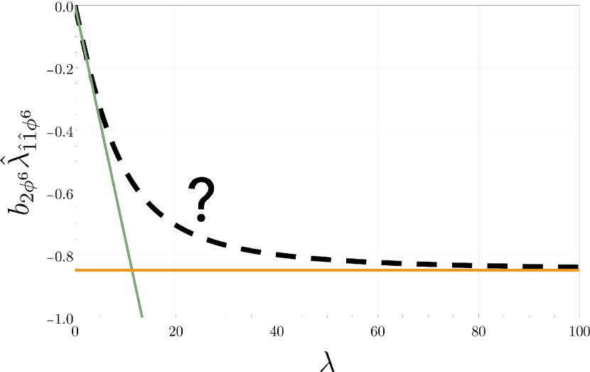
The strong-coupling limit of the topological sector can be evaluated using the already mentioned tools of Giombi:2018hsx . We focus ourselves here on the case , since it is the only one that we consider at strong coupling. It reads
| (61) |
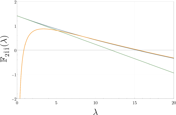
The topological sector at weak and strong coupling is plotted in Figure 3 for . Note that an exact expression is also provided in (78).
3.2 Superblock expansion
The constraints from superconformal symmetry discussed above can be used for deriving an expansion in superconformal blocks for the bulk-defect-defect correlators. Generically, the expansion in superconformal blocks (or superblocks) take the form
| (62) |
where designates the superprimary operators appearing in the OPE . For the case of the Wilson-line CFT, this OPE is given, e.g., in Ferrero:2023znz and reads
| (63) |
In the case , the leading contribution corresponds to the identity through the identification . The operators have unprotected scaling dimensions. The lowest-lying operator, both at weak and strong coupling, is , which has dimension Alday:2007hr ; Grabner:2020nis ; Cavaglia:2021bnz
| (64) | ||||
| (65) |
For , the content of the OPE is
| (66) |
In a perturbative setting, operators can become degenerate. The degeneracy grows with the tree-level scaling dimension . The large limit helps to reduce the degeneracy, but there are still many operators with the same tree-level scaling dimensions.444A counting of the number of operators can be found in Ferrero:2023znz .
From (66), we can read the expansion of in superblocks:
| (67) |
where in the last sum refers to the operators of .
We now discuss how to derive the explicit form of the superblocks. They can be decomposed into a -symmetry and a spacetime part through the following sum over the Dynkyn labels of the -symmetry and the scaling dimensions, here labelled as :
| (68) |
where refers to the bosonic blocks already introduced in (53). The range of the sums is determined by considering the content of the supermultiplets. This analysis was done in Ferrero:2023znz for the case of the Wilson-line defect CFT. We then apply the SCWI (56) on the blocks in order to fix the open coefficients . This amounts to requiring that individual blocks satisfy the symmetries of the correlator.
The identity block is simply given by
| (69) |
where the factor is there to account for the one present in the definition (48).
For the operator , we see in (B.4) of Ferrero:2023znz that the block should take the form
| (70) |
Note that we have selected scalar contributions in the supermultiplet. Generically, -symmetry blocks depend on the external operators, and for they are expected to take the form
| (71) |
where the coefficients are so far unfixed. Applying the SCWI (56) and choosing the normalization according to the highest-weight channel, we finally obtain
| (72) |
The same method can be applied for the superblocks of the long operators, yielding
| (73) |
The expansion in superblocks can be expanded in the coupling constant, through
| (74) |
and similarly for OPE coefficients. This allows a perturbative analysis, which will play an important role in Section 4. It is important however to notice that, as mentioned above, OPE coefficients and scaling dimensions become degenerate in a perturbative setting. Instead of individual coefficients, we are therefore forced to consider their average only. For instance,
| (75) |
where the sum is over all the operators that have the same tree-level scaling dimension . Note that we are using here the notation of Ferrero:2023znz . Moreover, the same analysis can be performed at strong coupling, and it is known that in this regime the degeneracy is being lifted slower than at weak coupling Liendo:2018ukf ; Ferrero:2021bsb .
The superblock expansion can be studied in the topological sector as well. It is well-known that only half-BPS contributions survive in this kinematic limit. For the case of , we have
| (76) |
This provides an exact formula for the topological sector discussed in Section 3.1.2. The average in the following sum corresponds to the contributions from the two operators and . This degeneracy is in fact absent, as it can be seen in the following way. Following the Gram-Schmidt procedure mentioned in above, the good operator takes the form
| (77) |
The corresponding OPE coefficient is of order . However the three-point function vanishes as a consequence of (77). The topological sector is therefore simply given by
| (78) |
This expression is plotted in Figure 3 from weak to strong coupling, using the analytic results (44), (43) and (37), and is shown to agree well with the perturbative results of Giombi:2018hsx .
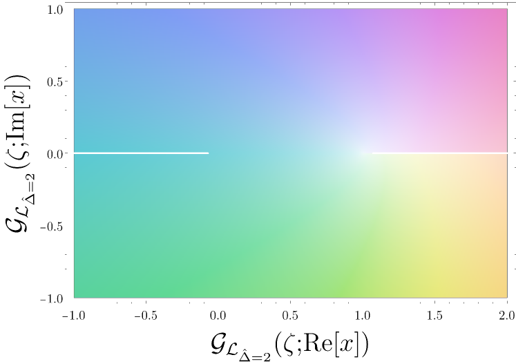
To conclude this section, let us make some remarks on the analytic structure of the conformal blocks. As noted in Levine:2023ywq ; Levine:2024wqn , conformal blocks are discontinuous at , which means that they do not satisfy locality on their own. This is shown in Figure 3. As a consequence, the (infinite) sum of superblocks should produce a function that is free of this discontinuity. This imposes strong constraints on the CFT data, which were studied in Levine:2023ywq ; Levine:2024wqn and formulated as sum rules.
3.3 Pinching and splitting limits
In this section, we present two kinematic limits corresponding to the reduction of some bulk-defect-defect correlators to simple functions, in particular to two-point bulk-defect functions (pinching limit) and products of one-point bulk correlators and two-point defect correlators (splitting limit). In our framework, lower-point functions serve as further non-perturbative information constraining the correlators under study.
3.3.1 Pinching limit
The pinching of the two defect operators into one having scaling dimension being the sum of the original two, i.e., the limit of the correlator and , results in the OPE coefficient after accounting for the different normalization constants:
| (79) |
with . This provides a valuable limit of the bulk-defect-defect correlator, since the coefficients can be evaluated (see (41)). If one inserts the expansion in channels (49) in (79), only the channel computed at survives:
| (80) |
from which it is possible to extract the pinching constraints at leading and next-to-leading orders:
| (81) | ||||
| (82) |
It might be tempting to consider another pinching limit, which consists in bringing the bulk operator in a third position on the line in order to generate a double-trace defect operator. This operator would however be of the form (27) and not orthonormal to the single-trace operators, as discussed in Section 3.1.2. Therefore, the fact that this pinching limit gives a non-vanishing result for is not an inconsistency with respect to (77), as this limit appears to be misleading at best.
3.3.2 Splitting limit
A different limit comes from considering a large separation between the bulk operator and the defect ones, i.e., . In the correlator expressed in symmetry channels (49), this corresponds to the limit of the whole correlator without setting (which would instead correspond to the previous pinching). In this case, the bulk-defect-defect correlator factorizes into a product of a two-point defect correlator and a one-point function of a bulk operator:
| (83) |
from which (49) simplifies to
| (84) |
where the coefficient is given in (44). This can serve as a constraint or consistency check for the case : Equation (84) combined with (49) gives
| (85) |
which is valid non-perturbatively.
4 Perturbative results
In this section, we present explicit results for the bulk-defect-defect correlators introduced in Section 2.2.3, and for which we listed non-perturbative constraints in Section 3. We begin by calculating correlators up to next-to-leading order at weak coupling. The results are obtained by combining the constraints mentioned above with simple calculations of Feynman diagrams that do not involve bulk vertices. For the case of , we determine the CFT data using the superblocks presented in Section 3.2. We observe that transcendental terms are systematically absent at this order, which results into relations for the OPE coefficients. We then consider the strong-coupling limit. We determine the contributions to the correlator up to next-to-leading order, and extract the corresponding CFT data. Finally, we present partial results for the next-to-next-to-leading order, for which one rational function remains unfixed but is shown to be strongly constrained by a collection of sum rules.
4.1 Weak coupling
4.1.1 Perturbative structure
At weak coupling, the bulk-defect-defect correlator has the following perturbative structure at large :
| (86) |
where the inside the brackets refer to higher powers of , while the at the end of the expression refer to corrections in . We focus mainly on this correlator in this section for ease of readability, before generalizing the expressions for arbitrary external dimensions in Section 4.1.4. As explained in (49), consists of two -symmetry channels:
| (87) |
4.1.2 Leading order
Correlator.
As a warm-up, let us determine the leading order for the case . This correlator consists of a single Feynman diagram, which can be represented as
| (88) |
and only consists of the free propagators defined in (9). It is easy to see that the -symmetry channels take the form
| (89) |
where is a constant that can be fixed either through direct calculation, the pinching constraint of (81) or the topological sector (58). At this order, we find
| (90) |
Note that the identity does not contribute at this order, i.e., we have
| (91) |
CFT data.
It is a trivial task to extract the CFT data for these results using the superblock expansion (67). For the long operators labelled as , we find the following closed form:
| (92) |
This is the supersymmetric version of the formula given in Levine:2023ywq ; Levine:2024wqn , and corresponding to an expansion in bosonic blocks.
4.1.3 Next-to-leading order
We now consider the next-to-leading order.
Correlator.
The Feynman diagrams corresponding to the correlator are listed in Table 1. Thanks to the non-perturbative constraints, we do not have to calculate all the diagrams. In particular, we can focus on the diagrams that do not contain bulk vertices. They are easy to compute using the integrals (154) and (155). We obtain
| (93) | ||||
| (94) |
where the prefactors result from symmetry factors and trace contributions. Note that each open line in (93)-(94) can end on the orange dots placed along the defect. Putting the two diagrams together, we obtain for the -symmetry channel the result
| (95) |
As a consistency test, we can check that this expression is compatible with the splitting constraint of Section 3.3:
| (96) |
The channel can be obtained through the supersymmetry constraints of Section 3.1. Using the solution (55) to the Ward identity, we obtain
| (97) |
Using the results of Giombi:2018hsx (summarized in Section 3.1.2), we can calculate the topological sector, and we get
| (98) |
The correlator is now completely fixed. Notice that this result was obtained without considering the second line of Table 1, where the Feynman diagrams consist of bulk vertices and are significantly harder than the first line. We calculated however these diagrams as a check of our results, and we found perfect agreement. This computation is reported in Appendix B.
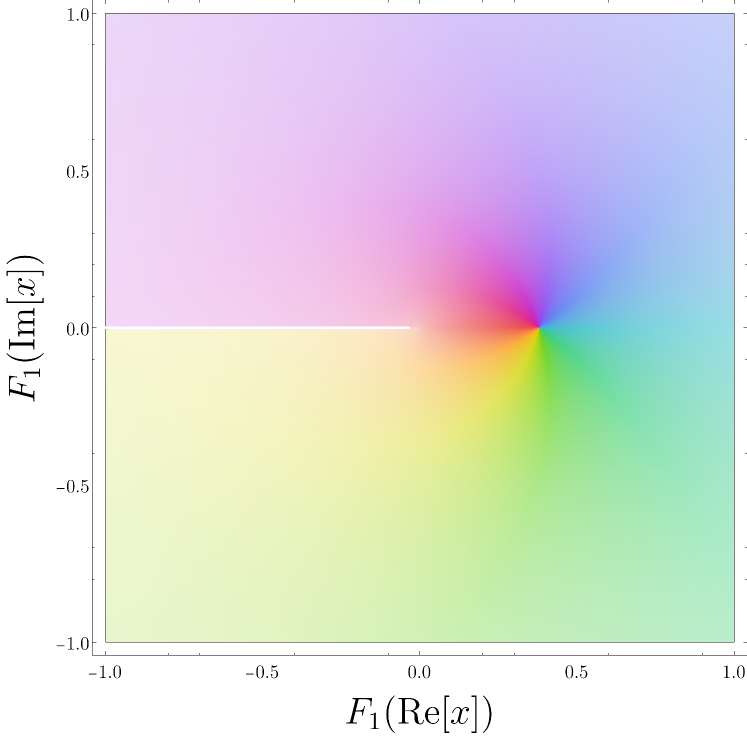
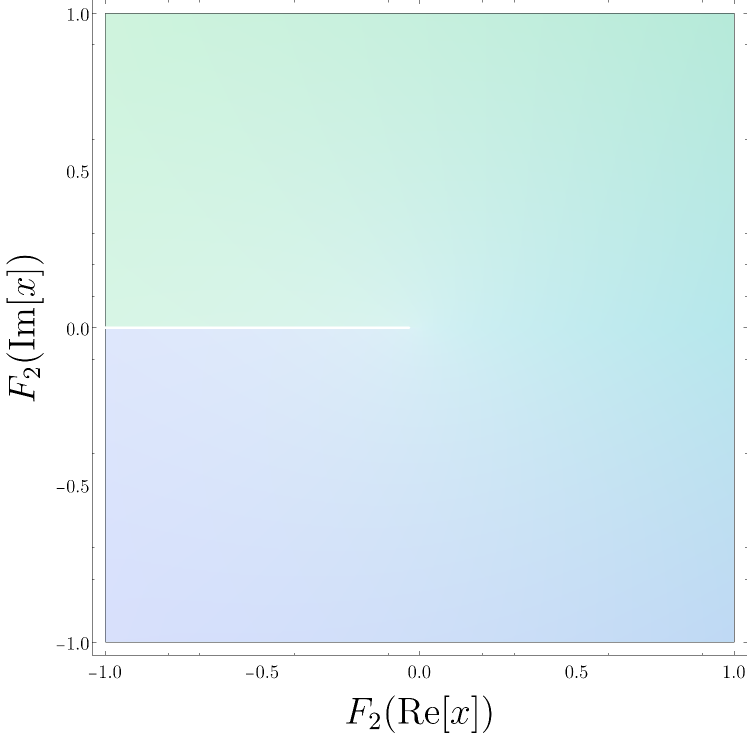
It is interesting to analyze the analytic structure of our results. It was shown in Levine:2023ywq ; Levine:2024wqn that, in order to satisfy locality constraints, bulk-defect-defect correlators should have a vanishing discontinuity at . Moreover, they are expected to have a branch cut at . The -symmetry channels and are plotted in Figure 4, where they are seen to satisfy these properties. Notice also that the individual diagrams of (93)-(94) do not satisfy the locality constraints, as can be seen in Figure 5.

CFT data.
The results above can be used for determining the CFT data at next-to-leading order. Notice that the expressions (95) and (97) are entirely rational, i.e., there are no transcendental functions appearing at this order. This is surprising, since we know that the operators exchanged in the OPE generally have anomalous dimensions at one loop, while we have seen in (92) that operators with even have a tree level OPE coefficient. This observation can be summarized in the following equation:
| (99) |
where the brackets should be understood in the average sense explained in (75) and below. We comment on the absence of logarithmic terms in Section 4.1.5.
In (92), we saw that operators with odd tree-level scaling dimension have vanishing OPE coefficients at order . They start to contribute at one loop, and we find the following closed form for their average:
| (100) |
with the harmonic numbers defined through
| (101) |
The lowest operator described by (100) corresponds to and is not degenerate. Its corresponding OPE coefficient is given by
| (102) |
Long operators with an even tree-level scaling dimension receive corrections to their tree-level value given in (92). It is difficult to find an analytic closed form, however they can be expressed in the form of a recursion relation:
| (103) |
Although this is not a closed form, note that recursion relations are extremely efficient, even for high . In the formula above, we used the Pochhammer symbols, defined through
| (104) |
4.1.4 Generalization to arbitrary , ,
We now repeat the analysis of the correlators presented above for the general case . We do not extract the CFT data, although we note that it is in principle possible to do it case by case in the same way as in Sections 4.1.2 and 4.1.3.
General Feynman diagrams.
We have seen in (88) and (93)-(94) that the correlator is fixed up to next-to-leading order by Feynman diagrams that do not contain bulk vertices. This observation holds for the general case . We are therefore interested in diagrams of the form
| (105) |
Here, the thick solid lines designate free propagators. The coefficients refer to the possible allowed contractions without involving a bulk vertex. They satisfy the consistency relations
| (106) |
Perturbative structure.
The Feynman diagrams (105) can be used to understand the perturbative structure of the bulk-defect-defect correlators. It is not hard to see that general correlators have to take the following form:
| (107) |
where we defined , i.e., the lowest number of propagators that can connect the bulk operators and the line defect for a given configuration characterized by , , , while still satisfying (106). The number of -symmetry channels can grow arbitrarily high, as can be seen in (50). However, at low orders, most of the -symmetry channels are suppressed for a given configuration. Concretely,
| (108) | ||||
| (109) | ||||
| (110) |
A new channel appears at each order until the full number of channels has been reached. In the following we study the correlators up to next-to-leading order, in which only two -symmetry channels contribute.
Leading order.
The leading order is given by the topological sector, since only one channel contributes and it is constant. To see that this is the case, consider the Feynman diagrams (105) for the distinct cases and . In the first case, there is no propagator connecting to the defect when minimizing , and thus the leading -symmetry channel is constant. The second configuration leads to considering to nested defect integrals. Using the identity (153), we can rewrite them in terms of a single master defect integral:
| (111) |
This integral is elementary and its solution is given by the sum of (154) and (155). The coefficient encodes the symmetry factors and the contributions from the traces. It is given by the topological sector (58), or the pinching limit (82) when applicable.
Next-to-leading order.
At next-to-leading order, we can use the supersymmetry constraint (55) and focus on calculating the channel only:
| (112) |
We only need to solve the generalized version of (93)-(94) in order to obtain all the correlators.
We can group the correlators into two different groups:
-
•
: These configurations are the ones where only one -symmetry channel exists. In this case, the correlator is topological and is equal to the topological sector .
-
•
: In the conformal frame , the only surviving diagrams are the ones depicted in (105), for which the value of is now raised by . The correlator can then be determined from the function
(113) which is the obvious generalization of (93)-(94). The sum over the signs means the presence of two summands with opposite signs. The constant is then fixed by the topological sector and pinching/splitting limits of Section 3.3.
4.1.5 On the absence of transcendental functions
We now comment on the absence of transcendental functions observed at next-to-leading order. In this setup, supersymmetry forces the combination of the Feynman diagrams gathered in Appendix B to form a rational function. It is unclear at present whether we should expect this property to appear in other theories. We provide in this section a few hints about this curious cancellation.
The first thing to notice is that, since we are dealing with OPE coefficients at leading order, we can restrict our operators to effective ones, i.e., operators that have spin and non-vanishing bulk-defect and three-point functions. Such operators are of the form
| (114) |
with a tensor structure This is required for the tree-level three-point functions to be potentially non-vanishing. The terms hidden in the might contribute however to .
Example for .
Let us illustrate Equation (99) for the OPE coefficient , to convince ourselves that it is not a trivial relation. From the correlator , we expect through (92) that
| (115) |
At , there are two operators contributing in the OPE which have the form (114). At one loop, they are defined as Correa:2018fgz
| (116) |
through orthogonalization of the anomalous dimension matrix. The one-loop anomalous dimensions are given by
| (117) |
From our results at leading order (see (92), we observe that
| (118) |
from which we conclude that
| (119) |
Moreover, we have argued in (114) that the two three-point function coefficients are equal. The equation (115) can then be written as
| (120) |
from which we can extract the disentangled data
| (121) |
It would be interesting to understand how this expression generalizes for higher-length operators, and if it persists for models without supersymmetry. We discuss this possibility further in Section 5.
4.2 Strong coupling
We now consider the bulk-defect-defect correlators in the strong-coupling regime. We provide the leading and next-to-leading orders with the corresponding CFT data for . At next-to-next-to-leading order, we determine through an Ansatz the transcendental part of the correlator, while the rational part is constrained by sum rules arising from locality.
4.2.1 Perturbative structure
We study the strong-coupling regime through a perturbative expansion at large of the form
| (122) |
For simplicity, we focus on . As in (86), the refer to corrections in inside the brackets and in outside the brackets. The relevant Witten diagrams are listed in Table 2, following the conventions of Figure 6, although we mostly use them as guides.
4.2.2 Leading order
At leading order, there is only one disconnected Witten diagram, which corresponds to the contribution of the identity operator. We have seen in Section 3.2 that the identity only appears in (in the form of a constant), and thus we have
| (123) |
The CFT data for the long operators is obviously
| (124) |
This expression is conservative, and in fact it is easy to convince oneself that individual operators have vanishing OPE coefficients:
| (125) |
4.2.3 Next-to-leading order
Witten diagram.
At next-to-leading order, there are two Witten diagrams contributing to the correlator, namely the second and third ones in Table 2. The first contribution is disconnected and corresponds to .555Note that the disconnected part can be evaluated at all orders in using the protected CFT data. The second one is the leading connected term, which consists only of free propagators. We therefore expect again the -symmetry channels to be constant. Moreover, this diagram corresponds, up to a prefactor, to the leading term of the bulk-defect correlator . This results in
| (126) |
Meanwhile, the disconnected term gives
| (127) |
CFT data.
We can easily extract the CFT data from this correlator. We first observe that the spectrum consists of defect operators with even scaling dimensions at tree level. This is in agreement with expectations from the AdS/CFT correspondence. For instance, the operator flows from at weak coupling to a two-particle state at strong coupling Alday:2007hr . Although the interpretation differs from weak coupling, the CFT data at leading order takes the same form up to an overall constant:
| (128) |
4.2.4 Partial results at next-to-next-to-leading order

We now discuss partial results for the next-to-next-to-leading order, in which we expect several Witten diagrams to appear. One example is the fourth diagram of Table 2. We give here the transcendental part of the correlator, as well as strong constraints on the remaining CFT data, in the form of sum rules.
Ansatz.
We start by formulating an Ansatz based on the expected structure of the correlator. In the strong-coupling regime, the transcendentality weight typically increases in steps of with powers of . Moreover, since we are dealing with a function of a single spacetime cross-ratio, this means that the correlator takes the following form at transcendentality one:
| (129) |
where the functions are rational functions (both at and ) as well as polynomials of degree one in in order to reflect the structure presented in (87):
| (130) |
Logarithmic terms.
We can obtain the log terms by using the fact that degeneracies are not lifted at next-to-leading order in the scaling dimensions.666See, e.g., Ferrero:2021bsb for an explanation and an application in four-point functions of defect operators. This means that we can extract the anomalous dimensions from the averages:
| (131) |
Note that this statement is assuming that the operators are single-trace. If we denote an arbitrary multi-trace operator of dimension by , we can convince ourselves that this is the case by noting that
| (132) |
Thus, at large , we only need to worry about , since three-point functions of defect multi-trace operators are suppressed. In fact, the coefficients and are seen to scale as by noting that
| (133) |
We are now in a similar situation to the one described below Equation (77): this scaling is true if the three-point function is non-vanishing. In fact, by requiring that is orthogonal to , we set at the same time , similarly to (77). To summarize, only single-trace operators appear in the left-hand side of (131). We believe this to be true at all orders in the coupling constant.777The statement above might still hold for higher-trace operators. The argument developed here is merely a way to circumvent the question.
Anomalous dimensions for the long operators are given by the quadratic Casimir eigenvalue for singlets of -symmetry and transverse spin:
| (134) |
Plugging these values inside the superblock expansion and comparing to the Ansatz (129), we find that the rational function corresponding to the log terms is given by
| (135) |
Topological sector.
We can further constrain the correlator by using the superconformal Ward identity. From the expression (55), we eliminate one of the two remaining rational functions through
| (136) |
The correlator at next-to-next-to-leading order is now fully fixed up to the rational function .
Sum rules.
We conclude this section by mentioning that the remaining rational function can in principle be further constrained from consistency conditions. The open rational function follows the superblock expansion
| (137) |
Strong constraints on these OPE coefficients can be derived by demanding locality, as it was shown in Levine:2023ywq . Since we are interested only in the rational terms, and that the terms are local, the coefficients of a corresponding bosonic block expansion are constrained by the sum rules
| (138) |
where is defined in Equation (3.27) of Levine:2023ywq . Here, is a positive integer assumed to be small but unknown. The sum rules alone are however insufficient for fixing all the coefficients if . Perhaps an input from the Witten diagram side can help to make the sum rules useful for fixing . We will not do this here, but mention interesting directions that can be followed with the sum rules in Section 5.
5 Conclusions
In this work, we have studied the correlation functions involving one bulk and two defect half-BPS operators in the context of the Wilson-line defect CFT in SYM. This setup preserves a lot of properties of SYM without defect, such as supersymmetry, integrability and a large subset of conformal symmetry. Through a combination of non-perturbative constraints and perturbative insights, we derived novel results for external operators with arbitrary scaling dimensions at weak coupling. At next-to-leading order, we observe a cancellation of transcendental terms. This is explained through intricate relations between the OPE coefficients and the scaling dimensions, which follows from supersymmetry. It is unclear what the fate of this observation is in other models. In the strong-coupling regime, we provide results for the correlator up to next-to-leading order, and present partial results for the next-to-next-to-leading order contribution. In this case, the correlator is known up to a rational function of the spacetime cross-ratio, which is further constrained through sum rules in the gist of Levine:2023ywq .
There are many interesting directions that one can take after this work. We list here some that we find particularly promising:
-
•
In the weak coupling regime, little is known about the functional space of these correlators. In the case of the Wilson line in SYM, we encounter trigonometric functions of the spacetime cross-ratio , which are rational for the whole range . This is not surprising, as is directly related to the angle formed by the two defect operators while keeping the bulk operator fixed. It would be interesting to study the integrals encountered at next-to-next-to-leading order using the variable , and see if it leads to simplifications. A valuable tool to further constrain the result once understood the space of functions can be locality, in the spirit of the discontinuity analysis presented in Levine:2023ywq . As Fig. 5 shows, the functions appearing as the result of individual Feynman diagrams can have non-physical branch cuts: if the space of functions is known, applying locality constraints can partially fix the contribution from other diagrams, as non-physical discontinuities must cancel;
-
•
We observe a surprising cancellation of the transcendental terms at next-to-leading order. Although this can be explained through relations between the OPE coefficients, it would be valuable to gain a deeper insight into the reasons that prevent logarithms to appear, in particular to see if supersymmetry is responsible for this cancellation. One idea is to consider the bulk-defect-defect correlator of the lowest-lying operators in the model, using the -expansion at the Wilson-Fisher fixed point (see Cuomo:2021kfm ; Gimenez-Grau:2022czc ; Gimenez-Grau:2022ebb ; Bianchi:2022sbz ; Pannell:2023pwz ; Giombi:2023dqs for related works). At next-to-leading order, a single diagram contributes:
(139) We observe in this case as well an absence of transcendental terms, which might hint at a more universal mechanism that does not involve supersymmetry. This can be investigated systematically by considering different models (e.g. fishnet field theory in presence of a defect Wu:2020nis ; Gromov:2021ahm or fermionic defect CFT Giombi:2022vnz ; Barrat:2023ivo ; Pannell:2023pwz ) and different external operators;
-
•
The sum rules presented in Levine:2023ywq are amenable to a numerical study, especially in this case where the spectrum is known through integrability throughout the conformal manifold Cavaglia:2021bnz ; Cavaglia:2022qpg ; Cavaglia:2022yvv . Typical bootstrap strategies are however suffering from the fact that the OPE coefficients are not positive, as it is the case for four-point functions of identical operators. An alternative method would be to truncate the sum à la Gliozzi Gliozzi:2016cmg and use an adapted version of the Tauberian theorem to estimate the tail, similarly to what was done in thermal cases Qiao:2017xif ; Marchetto:2023fcw ; Barrat:2024aoa . It would also be interesting to see a full-fledged bootstrap study of a defect CFT that involves the four-point functions of defect operators , the two-point functions of bulk operators (in presence of the defect) , together with the bulk-defect-defect correlators . This should result in intertwining relations that might provide interesting relations for lifting degeneracies in perturbative settings. A good candidate of an observable to study numerically and that appears in is the combination (see Figure 8). The three-point function has been studied extensively and is known precisely from weak to strong coupling, up to a sign, while presently very little is known about . The numerical approach would also profit from integrated correlator relations, such as the ones derived for SYM in Dorigoni:2022zcr ; Alday:2023pet and for line defects in Drukker:2022pxk ; Cavaglia:2022qpg ; Cavaglia:2022yvv ; Pufu:2023vwo .
Acknowledgements.
We are particularly grateful to Lorenzo Bianchi, Gabriel Bliard, Valentina Forini, Philine Van Vliet for useful discussions. DA and YX are funded by the Deutsche Forschungsgemeinschaft (DFG, German Research Foundation) – Projektnummer 417533893/GRK2575 “Rethinking Quantum Field Theory”. JB is supported by ERC-2021-CoG - BrokenSymmetries 101044226, and has benefited from the German Research Foundation DFG under Germany’s Excellence Strategy – EXC 2121 Quantum Universe – 390833306. DA is especially grateful to the organizers of the workshop Defects, from condensed matter to quantum gravity for providing the framework for useful discussions.Appendix A Integrals
A.1 Bulk integrals
We gather here the bulk integrals used throughout this work. We often encounter the well-known X-integral, for which the definition and the solution are
| (140) |
where we have used the Bloch-Wigner function bloch1978applications , defined as
| (141) |
Here the cross-ratios and are related to the coordinates of the external points in the standard way:
| (142) |
Note that the Bloch-Wigner function is crossing symmetric:
| (143) |
If two external points are coincident, the X-integral becomes divergent. It can be expressed in the following way:
| (144) |
where the integral is given in (147).
We also encounter the Y-integral, which can be obtained through the limit of the X-integral:
| (145) |
The cross-ratios are now defined as
| (146) |
The Y-integral is log-divergent in the limit where two external points are coincident. The corresponding expression is given by
| (147) |
Note that we use point-splitting regularization. The Y-integral is often encountered with derivatives. The following identities are useful for manipulating the integrals:
| (148) |
where we have use the scalar Green’s equation
| (149) |
It is useful to define the following integral:
| (150) |
where we have introduced the shorthand notation . This integral is encountered in Feynman diagrams with two gluon vertices. It can be expressed in terms of X- and Y-integrals Beisert:2002bb :
| (151) |
The F-integral is also log-divergent in the coincident limit:
| (152) |
A.2 Defect integrals
We present here explicitly the defect integrals necessary to compute the bulk-defect-defect correlators at NLO. The diagrams appearing in the channel do not have bulk vertices, therefore the integrals arise from the coupling of with the Wilson line
| (153) |
and similar from a point to . Equation (153) implies that the only integrals determining bulk-defect-defect correlators as next-to-leading order are
| (154) |
and
| (155) |
Appendix B Check through Feynman diagrams
We present here the results for the Feynman diagrams of Table 1 that contribute to the channel of the correlator . The results are obtained using the Feynman rules of Section 2.1.2 and the integrals of Appendix A.
B.1 Self-energy diagrams
We begin by the self-energy diagrams. Using the insertion rule (14), it is easy to find that
| (156) |
while
| (157) |
Note that these results are given in the conformal limit . In other words, each diagram contains corrections in , however since we know that the correlator depends on a single cross-ratio , they are expected to cancel once added up. As visible in the final result (97), we observe indeed a cancellation of the terms.
B.2 Diagrams with bulk vertices
There are two diagrams that involve bulk vertices but no integration along the Wilson line. The first one contains the X-integral defined in (140), and pinched to (144). Taking into account all the prefactors, it reads
| (158) |
The second diagram involves the F-integral (150). Using (152), we obtain
| (159) |
B.3 Boundary diagrams
Finally, there are two diagrams that involve an integral along the Wilson line, as well as a bulk vertex. These integrals are more challenging but can be performed analytically in the conformal frame . The first one gives
| (160) |
where it should be understood that the gluon propagator can connect to each orange dot on the line. The second one yields
| (161) |
When adding all the diagrams, we find that the divergences cancel as well as the terms. The result is in perfect agreement with 97.
References
- (1) S. Caron-Huot, Analyticity in Spin in Conformal Theories, JHEP 09 (2017) 078 [1703.00278].
- (2) D. Carmi and S. Caron-Huot, A Conformal Dispersion Relation: Correlations from Absorption, JHEP 09 (2020) 009 [1910.12123].
- (3) J. M. Maldacena, The Large N limit of superconformal field theories and supergravity, Adv. Theor. Math. Phys. 2 (1998) 231 [hep-th/9711200].
- (4) J. M. Maldacena, Wilson loops in large N field theories, Phys. Rev. Lett. 80 (1998) 4859 [hep-th/9803002].
- (5) A. M. Polyakov, Thermal Properties of Gauge Fields and Quark Liberation, Phys. Lett. B 72 (1978) 477.
- (6) E. Witten, Anti-de Sitter space, thermal phase transition, and confinement in gauge theories, Adv. Theor. Math. Phys. 2 (1998) 505 [hep-th/9803131].
- (7) J. Barrat, A. Gimenez-Grau and P. Liendo, Bootstrapping holographic defect correlators in = 4 super Yang–Mills, JHEP 04 (2022) 093 [2108.13432].
- (8) J. Barrat, A. Gimenez-Grau and P. Liendo, A dispersion relation for defect CFT, JHEP 02 (2023) 255 [2205.09765].
- (9) L. Bianchi and D. Bonomi, Conformal dispersion relations for defects and boundaries, 2205.09775.
- (10) A. Gimenez-Grau, The Witten Diagram Bootstrap for Holographic Defects, 2306.11896.
- (11) J. Barrat, P. Liendo and J. Plefka, Two-point correlator of chiral primary operators with a Wilson line defect in = 4 SYM, JHEP 05 (2021) 195 [2011.04678].
- (12) N. Drukker, S. Giombi, R. Ricci and D. Trancanelli, Wilson loops: From four-dimensional SYM to two-dimensional YM, Phys. Rev. D 77 (2008) 047901 [0707.2699].
- (13) S. Giombi and V. Pestun, Correlators of local operators and 1/8 BPS Wilson loops on S**2 from 2d YM and matrix models, JHEP 10 (2010) 033 [0906.1572].
- (14) S. Giombi and V. Pestun, The 1/2 BPS ’t Hooft loops in N=4 SYM as instantons in 2d Yang–Mills, J. Phys. A 46 (2013) 095402 [0909.4272].
- (15) E. I. Buchbinder and A. A. Tseytlin, Correlation function of circular Wilson loop with two local operators and conformal invariance, Phys. Rev. D 87 (2013) 026006 [1208.5138].
- (16) M. Beccaria and A. A. Tseytlin, On the structure of non-planar strong coupling corrections to correlators of BPS Wilson loops and chiral primary operators, JHEP 01 (2021) 149 [2011.02885].
- (17) A. Cavaglià, N. Gromov, J. Julius and M. Preti, Integrability and conformal bootstrap: One dimensional defect conformal field theory, Phys. Rev. D 105 (2022) L021902 [2107.08510].
- (18) A. Cavaglià, N. Gromov, J. Julius and M. Preti, Bootstrability in defect CFT: integrated correlators and sharper bounds, JHEP 05 (2022) 164 [2203.09556].
- (19) A. Cavaglià, N. Gromov, J. Julius and M. Preti, Integrated correlators from integrability: Maldacena-Wilson line in = 4 SYM, JHEP 04 (2023) 026 [2211.03203].
- (20) A. Cavaglià, N. Gromov and M. Preti, Computing Four-Point Functions with Integrability, Bootstrap and Parity Symmetry, 2312.11604.
- (21) S. Giombi, R. Roiban and A. A. Tseytlin, Half-BPS Wilson loop and AdS2/CFT1, Nucl. Phys. B 922 (2017) 499 [1706.00756].
- (22) S. Giombi, S. Komatsu, B. Offertaler and J. Shan, Boundary reparametrizations and six-point functions on the AdS2 string, JHEP 08 (2024) 196 [2308.10775].
- (23) P. Liendo and C. Meneghelli, Bootstrap equations for = 4 SYM with defects, JHEP 01 (2017) 122 [1608.05126].
- (24) P. Liendo, C. Meneghelli and V. Mitev, Bootstrapping the half-BPS line defect, JHEP 10 (2018) 077 [1806.01862].
- (25) P. Ferrero and C. Meneghelli, Bootstrapping the half-BPS line defect CFT in N=4 supersymmetric Yang–Mills theory at strong coupling, Phys. Rev. D 104 (2021) L081703 [2103.10440].
- (26) P. Ferrero and C. Meneghelli, Unmixing the Wilson line defect CFT. Part I. Spectrum and kinematics, JHEP 05 (2024) 090 [2312.12550].
- (27) P. Ferrero and C. Meneghelli, Unmixing the Wilson line defect CFT. Part II. Analytic bootstrap, JHEP 06 (2024) 010 [2312.12551].
- (28) S. Giombi and S. Komatsu, Exact Correlators on the Wilson Loop in SYM: Localization, Defect CFT, and Integrability, JHEP 05 (2018) 109 [1802.05201].
- (29) J. Barrat, P. Liendo, G. Peveri and J. Plefka, Multipoint correlators on the supersymmetric Wilson line defect CFT, JHEP 08 (2022) 067 [2112.10780].
- (30) J. Barrat, P. Liendo and G. Peveri, Multipoint correlators on the supersymmetric Wilson line defect CFT II: Unprotected operators, 2210.14916.
- (31) G. Bliard, On multipoint Ward identities for superconformal line defects, 2405.15846.
- (32) J. Barrat, C. Meneghelli and S. Müller, work in progress, To appear .
- (33) G. J. S. Bliard, Perturbative and non-perturbative analysis of defect correlators in AdS/CFT, Ph.D. thesis, Humboldt U., Berlin, 2023. 2310.18137. 10.18452/27559.
- (34) G. Peveri, Correlators on the Wilson Line Defect CFT, Ph.D. thesis, Humboldt U., Berlin, 2023. 2310.17358. 10.18452/27524.
- (35) J. Barrat, Line defects in conformal field theory, Ph.D. thesis, Humboldt U., Berlin, Humboldt-Universität zu Berlin, 2024. 2401.10336. 10.18452/28278.
- (36) J. Barrat, G. Bliard, P. Ferrero, C. Meneghelli and G. Peveri, Bootstrapping multipoint correlators on the Wilson line defect CFT, To appear .
- (37) E. Lauria, P. Liendo, B. C. Van Rees and X. Zhao, Line and surface defects for the free scalar field, JHEP 01 (2021) 060 [2005.02413].
- (38) N. Levine and M. F. Paulos, Bootstrapping bulk locality. Part I: Sum rules for AdS form factors, JHEP 01 (2024) 049 [2305.07078].
- (39) N. Levine and M. F. Paulos, Bootstrapping bulk locality. Part II: Interacting functionals, 2408.00572.
- (40) I. Burić and V. Schomerus, Defect Conformal Blocks from Appell Functions, JHEP 05 (2021) 007 [2012.12489].
- (41) Y. Okuyama, Aspects of critical O model with boundary and defect, other thesis, 1, 2024.
- (42) A. Gimenez-Grau, P. Liendo and P. van Vliet, Superconformal boundaries in dimensions, JHEP 04 (2021) 167 [2012.00018].
- (43) S. Giombi and S. Komatsu, More Exact Results in the Wilson Loop Defect CFT: Bulk-Defect OPE, Nonplanar Corrections and Quantum Spectral Curve, J. Phys. A 52 (2019) 125401 [1811.02369].
- (44) R. D’Auria, P. Fre and A. J. da Silva, Geometric Structure of and Superyang-mills Theory, Nucl. Phys. B 196 (1982) 205.
- (45) J. K. Erickson, G. W. Semenoff and K. Zarembo, Wilson loops in N=4 supersymmetric Yang–Mills theory, Nucl. Phys. B 582 (2000) 155 [hep-th/0003055].
- (46) G. W. Semenoff and K. Zarembo, Wilson loops in SYM theory: From weak to strong coupling, Nucl. Phys. B Proc. Suppl. 108 (2002) 106 [hep-th/0202156].
- (47) S. Lee, S. Minwalla, M. Rangamani and N. Seiberg, Three point functions of chiral operators in D = 4, N=4 SYM at large N, Adv. Theor. Math. Phys. 2 (1998) 697 [hep-th/9806074].
- (48) N. Drukker and J. Plefka, The Structure of n-point functions of chiral primary operators in N=4 super Yang–Mills at one-loop, JHEP 04 (2009) 001 [0812.3341].
- (49) N. Drukker and J. Plefka, Superprotected n-point correlation functions of local operators in N=4 super Yang–Mills, JHEP 04 (2009) 052 [0901.3653].
- (50) C. Bercini, B. Fernandes and V. Goncalves, Two loop five point integrals: light, heavy and large spin correlators, 2401.06099.
- (51) J. Barrat, A. Gimenez-Grau and P. Liendo, Unpublished notes, .
- (52) F. A. Dolan and H. Osborn, Superconformal symmetry, correlation functions and the operator product expansion, Nucl. Phys. B 629 (2002) 3 [hep-th/0112251].
- (53) F. A. Dolan and H. Osborn, Conformal partial wave expansions for N=4 chiral four point functions, Annals Phys. 321 (2006) 581 [hep-th/0412335].
- (54) F. A. Dolan, L. Gallot and E. Sokatchev, On four-point functions of 1/2-BPS operators in general dimensions, JHEP 09 (2004) 056 [hep-th/0405180].
- (55) L. F. Alday and J. M. Maldacena, Gluon scattering amplitudes at strong coupling, JHEP 06 (2007) 064 [0705.0303].
- (56) D. Grabner, N. Gromov and J. Julius, Excited States of One-Dimensional Defect CFTs from the Quantum Spectral Curve, JHEP 07 (2020) 042 [2001.11039].
- (57) D. Correa, M. Leoni and S. Luque, Spin chain integrability in non-supersymmetric Wilson loops, JHEP 12 (2018) 050 [1810.04643].
- (58) G. Cuomo, Z. Komargodski and M. Mezei, Localized magnetic field in the O(N) model, JHEP 02 (2022) 134 [2112.10634].
- (59) A. Gimenez-Grau, E. Lauria, P. Liendo and P. van Vliet, Bootstrapping line defects with O(2) global symmetry, JHEP 11 (2022) 018 [2208.11715].
- (60) A. Gimenez-Grau, Probing magnetic line defects with two-point functions, 2212.02520.
- (61) L. Bianchi, D. Bonomi and E. de Sabbata, Analytic bootstrap for the localized magnetic field, JHEP 04 (2023) 069 [2212.02524].
- (62) W. H. Pannell and A. Stergiou, Line defect RG flows in the expansion, JHEP 06 (2023) 186 [2302.14069].
- (63) S. Giombi and B. Liu, Notes on a Surface Defect in the Model, 2305.11402.
- (64) J.-b. Wu, J. Tian and B. Chen, Loop operators in three-dimensional = 2 fishnet theories, JHEP 07 (2020) 215 [2004.07592].
- (65) N. Gromov, J. Julius and N. Primi, Open fishchain in N = 4 Supersymmetric Yang-Mills Theory, JHEP 07 (2021) 127 [2101.01232].
- (66) S. Giombi, E. Helfenberger and H. Khanchandani, Line Defects in Fermionic CFTs, 2211.11073.
- (67) J. Barrat, P. Liendo and P. van Vliet, Line defect correlators in fermionic CFTs, 2304.13588.
- (68) F. Gliozzi, Truncatable bootstrap equations in algebraic form and critical surface exponents, JHEP 10 (2016) 037 [1605.04175].
- (69) J. Qiao and S. Rychkov, A tauberian theorem for the conformal bootstrap, JHEP 12 (2017) 119 [1709.00008].
- (70) E. Marchetto, A. Miscioscia and E. Pomoni, Broken (super) conformal Ward identities at finite temperature, 2306.12417.
- (71) J. Barrat, B. Fiol, E. Marchetto, A. Miscioscia and E. Pomoni, Conformal line defects at finite temperature, 2407.14600.
- (72) D. Dorigoni, M. B. Green and C. Wen, Exact results for duality-covariant integrated correlators in SYM with general classical gauge groups, SciPost Phys. 13 (2022) 092 [2202.05784].
- (73) L. F. Alday, S. M. Chester, D. Dorigoni, M. B. Green and C. Wen, Relations between integrated correlators in = 4 supersymmetric Yang-Mills theory, JHEP 05 (2024) 044 [2310.12322].
- (74) N. Drukker, Z. Kong and G. Sakkas, Broken Global Symmetries and Defect Conformal Manifolds, Phys. Rev. Lett. 129 (2022) 201603 [2203.17157].
- (75) S. S. Pufu, V. A. Rodriguez and Y. Wang, Scattering From -Strings in , 2305.08297.
- (76) S. Bloch, Applications of the dilogarithm function in algebraic K-theory and algebraic geometry, in Proc. of the Int. Symp. on Algebraic Geometry, Kyoto, 1977, Kinokuniya, Tokyo, 1978, 1978.
- (77) N. Beisert, C. Kristjansen, J. Plefka, G. W. Semenoff and M. Staudacher, BMN correlators and operator mixing in N=4 superYang–Mills theory, Nucl. Phys. B 650 (2003) 125 [hep-th/0208178].