DART: Denoising Autoregressive Transformer for Scalable Text-to-Image Generation

Abstract

Diffusion models have become the dominant approach for visual generation. They are trained by denoising a Markovian process which gradually adds noise to the input. We argue that the Markovian property limits the model’s ability to fully utilize the generation trajectory, leading to inefficiencies during training and inference. In this paper, we propose DART, a transformer-based model that unifies autoregressive (AR) and diffusion within a non-Markovian framework. DART iteratively denoises image patches spatially and spectrally using an AR model that has the same architecture as standard language models. DART does not rely on image quantization, which enables more effective image modeling while maintaining flexibility. Furthermore, DART seamlessly trains with both text and image data in a unified model. Our approach demonstrates competitive performance on class-conditioned and text-to-image generation tasks, offering a scalable, efficient alternative to traditional diffusion models. Through this unified framework, DART sets a new benchmark for scalable, high-quality image synthesis.

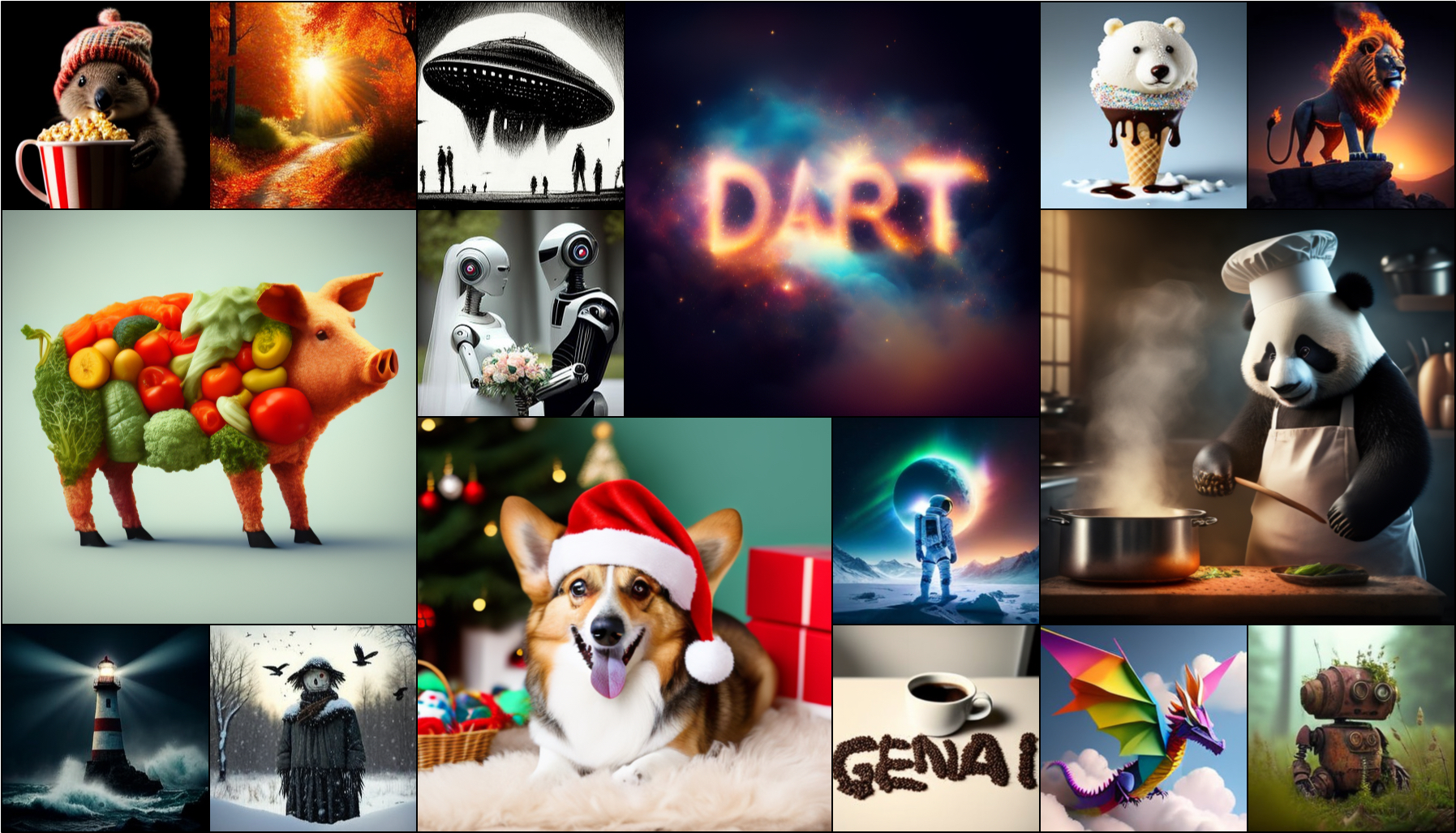
Figure 1: Curated examples of images generated by DART at $256\times 256$ and $512\times 512$ pixels.

1 Introduction

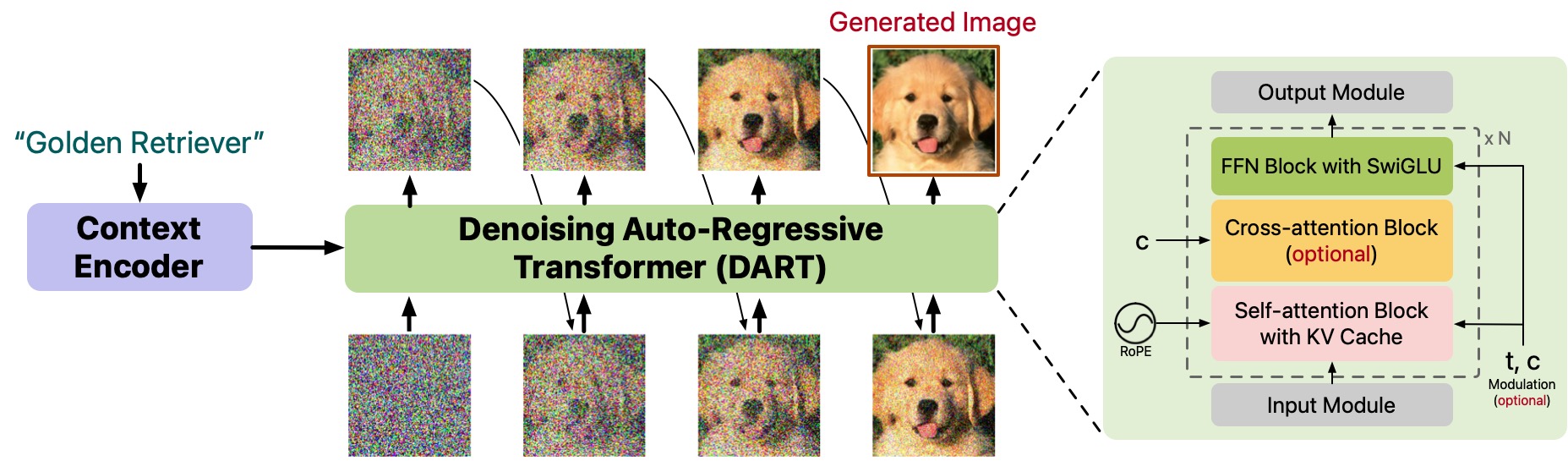
Figure 2: ($\leftarrow$) A general illustration of the proposed DART. The model autoregressively denoises image through a Transformer until a clean image is generated. Here, whole images are shown for visualization purpose; ($\rightarrow$) We show the architecture details which integrates state-of-the-art designs similar to common language models (Dubey et al., 2024).

Recent advancements in deep generative models have led to significant breakthroughs in visual synthesis, with diffusion models emerging as the dominant approach for generating high-quality images (Rombach et al., 2022; Esser et al., 2024). Diffusion models (Sohl-Dickstein et al., 2015; Ho et al., 2020) operate by progressively adding Gaussian noise to an image and learning to reverse this process in a sequence of denoising steps. Despite their success, these models are difficult to train on high resolution images directly, requiring either cascaded models (Ho et al., 2022), or multiscale approaches (Gu et al., 2023) or preprocessing of images to autoencoder codes at lower resolutions (Rombach et al., 2022). These limitations can stem from their reliance on the Markovian assumption, which simplifies the generative process but restricts the model only to see the generation from the previous step. This often leads to inefficiencies during training and inference, as the individual steps of denoising are unaware of the trajectory of generations from prior steps.

In parallel, autoregressive models, such as GPT-4 (Achiam et al., 2023), have shown great success in modeling long-range dependencies in sequential data, particularly in the field of natural language processing. These models efficiently cache computations and manage dependencies across time steps, which has also inspired research into adapting autoregressive models for image generation. Early efforts such as PixelCNN (Oord et al., 2016) suffered from high computational costs due to pixel-wise generation. More recent models like VQ-GAN (Esser et al., 2021) and related work (Yu et al., 2022; Team, 2024; Tian et al., 2024) learn models of quantized images in a compressed latent space; Li et al. (2024) propose to generate directly in such space without quantization by employing a diffusion-based loss function. However, these methods fail to fully leverage the progressive denoising benefits of diffusion models, resulting in limited global context and error propagation during generation.

To address these limitations, we propose Denoising AutoRegressive Transformer (DART), a novel generative model that integrates autoregressive modeling within a non-Markovian diffusion framework (Song et al., 2021) (Fig. 2). The non-Markovian formulation in DART enables the model to leverage the full generative trajectory during training and inference, while retaining the progressive modeling benefits of diffusion models, resulting in more efficient and flexible generation compared to traditional diffusion and autoregressive approaches. Additionally, DART introduces two key improvements to address the limitations of the non-Markovian approach: (1) token-level autoregressive modeling (DART-AR), which captures dependencies between image tokens autoregressively, enabling finer control and improved generation quality, and (2) a flow-based refinement module (DART-FM), which enhances the model’s expressiveness and smooths transitions between denoising steps. These extensions make DART a flexible and efficient framework capable of handling a wide range of tasks, including class conditional, text-to-image, as well as multimodal generation.

DART offers a scalable, efficient alternative to traditional diffusion models, achieving competitive performance on standard benchmarks for class-conditioned (e.g., ImageNet (Deng et al., 2009)) and text-to-image generation. To summarize, major contributions of our work include:

• We propose DART, a novel non-Markovian diffusion model that leverages the full denoising trajectory, leading to more efficient and flexible image generation compared to traditional approaches.

• We propose two key improvements: DART-AR and DART-FM, which improve the expressiveness and coherence throughout the non-Markovian generation process.

• DART achieves competitive performance in both class-conditioned and text-to-image generation tasks, offering a scalable and unified approach for high-quality, controllable image synthesis.

2 Background

2.1 Diffusion Models

Diffusion models (Sohl-Dickstein et al., 2015; Ho et al., 2020; Song et al., 2020) are latent variable models with a fixed posterior distribution, and trained with a denoising objective. These models have gained widespread use in image generation (Rombach et al., 2021; Podell et al., 2023; Esser et al., 2024). Diffusion models produce the entire image in a non-autoregressive manner through iterative processes. Specifically, given an image ${\bm{x}}_{0}\in\mathbb{R}^{3\times H\times W}$, we define a series of latent variables ${\bm{x}}_{t}$ ($t=1,\cdots,T$) with a Markovian process which gradually adds noise to the original image ${\bm{x}}_{0}$. The transition $q({\bm{x}}_{t}|{\bm{x}}_{t-1})$ and the marginal $q({\bm{x}}_{t}|{\bm{x}}_{0})$ probabilities are defined as follows, respectively:

$$q({\bm{x}}_{t}|{\bm{x}}_{t-1})=\mathcal{N}({\bm{x}}_{t};\sqrt{1-\beta_{t}}{\bm{x}}_{t-1},\beta_{t}\mathbf{I}),\;\;q({\bm{x}}_{t}|{\bm{x}}_{0})=\mathcal{N}({\bm{x}}_{t};\sqrt{\bar{\alpha}_{t}}{\bm{x}}_{0},\left(1-\bar{\alpha}_{t}\right)\mathbf{I}),$$ (1)

where $\bar{\alpha}_{t}=\prod_{\tau=1}^{t}(1-\beta_{\tau}),0<\beta_{t}<1$ are determined by the noise schedule. The model learns to reverse this process with a backward model $p_{\theta}({\bm{x}}_{t-1}|{\bm{x}}_{t})$, which aims to denoise the image. The training objective for the model is:

$$\min\mathcal{L}_{\theta}^{\text{DM}}=\mathbb{E}_{t\sim[1,T],{\bm{x}}_{t}\sim q({\bm{x}}_{t}|{\bm{x}}_{0})}[\omega_{t}\cdot\|{\bm{x}}_{\theta}({\bm{x}}_{t},t)-{\bm{x}}_{0}\|_{2}^{2}],$$ (2)

where ${\bm{x}}_{\theta}({\bm{x}}_{t},t)$ is a time-conditioned denoiser that learns to map the noisy sample ${\bm{x}}_{t}$ to its clean version ${\bm{x}}_{0}$; $\omega_{t}$ is a time-dependent loss weighting, which usually uses SNR (Ho et al., 2020) or SNR+1 (Salimans & Ho, 2022). Practically, ${\bm{x}}_{t}$ can be re-parameterized with noise- or v-prediction (Salimans & Ho, 2022) for enhanced performance, and can be applied on pixel space (Gu et al., 2023; Saharia et al., 2022) or latent space, encoded by a VAE encoder (Rombach et al., 2021). However, standard diffusion models are computationally inefficient, requiring numerous denoising steps and extensive training data. Moreover, they lack the ability to leverage generation context effectively, hindering scalability to complex scenes and long sequences like videos.

2.2 Autoregressive Models

In the field of natural language processing, Transformer models have achieved notable success in autoregressive modeling (Vaswani et al., 2017b; Raffel et al., 2020). Building on this success, similar approaches have been applied to image generation (Parmar et al., 2018; Esser et al., 2021; Chen et al., 2020; Yu et al., 2022; Sun et al., 2024; Team, 2024). Different from diffusion-based methods, these methods typically focus on learning the dependencies among discrete image tokens (e.g., through Vector Quantization (Van Den Oord et al., 2017)). To elaborate, consider an image ${\bm{x}}\in\mathbb{R}^{3\times H\times W}$. The process begins by encoding this image into a sequence of discrete tokens ${\bm{z}}_{1:N}=\mathcal{E}({\bm{x}})$. These tokens are designed to approximately reconstruct the original image through a learned decoder $\hat{{\bm{x}}}=\mathcal{D}({\bm{z}}_{1:N})$. An autoregressive model is then trained by maximizing the cross-entropy as follows:

$$\max\mathcal{L}_{\theta}^{\textrm{CE}}=\sum_{n=1}^{N}\log P_{\theta}({\bm{z}}_{n}|{\bm{z}}_{0:n-1}),$$ (3)

where ${\bm{z}}_{0}$ is the special start token. During the inference phase, the autoregressive model is first used to sample tokens from the learned distribution, and then decode them into image space using $\mathcal{D}$.

As discussed in Kilian et al. (2024), autoregressive models offer significant efficiency advantages over diffusion models by caching previous steps in memory and enabling the entire generation process to be computed in a single parallel forward pass. This reduces computational overhead and accelerates training and inference. However, the reliance on quantization can lead to information loss, potentially degrading generation quality. Additionally, the linear, step-by-step nature of token prediction may overlook the global structure, making it challenging to capture long-range dependencies and holistic coherence in complex scenes or sequences.

3 DART

3.1 Non-Markovian Diffusion Formulation

We start by revisiting the basics of diffusion models from the perspective of hierarchical variational auto-encoders (HVAEs, Kingma & Welling, 2013; Child, 2021). Given a data-point ${\bm{x}}_{0}$, a HVAE process $p_{\theta}$ of a sequence of latent variables $\{{\bm{x}}_{t}\}_{t}$ by maximizing a evidence lower bound (ELBO):

$$\max\mathcal{L}^{\text{ELBO}}_{\theta,\phi}=\mathbb{E}_{{\bm{x}}_{1:T}\sim q_{\phi}({\bm{x}})}\left[\sum_{t=1}^{T}\log p_{\theta}({\bm{x}}_{t-1}|{\bm{x}}_{t:T})+\log p_{\theta}({\bm{x}}_{T})-\log q_{\phi}({\bm{x}}_{1:T}|{\bm{x}}_{0})\right],$$ (4)

where ${\bm{x}}_{0}$ is the real data, and $q_{\phi}$ is a learnable inference model. As pointed out in VDM (Kingma et al., 2021), diffusion models can essentially be seen as HVAEs with three specific modifications:

1. A fixed inference process $q$ which gradually adds noise to corrupt data ${\bm{x}}_{0}$;

2. Markovian forward and backward process where ${\bm{x}}_{t}$ depends only on ${\bm{x}}_{t+1}$ (Eq 1);

3. Noise-dependent loss weighting that reweighs ELBO with a focus on perception.

Only with all above simplifications combined, standard diffusion models can be formulated as Eq 2 where the generator becomes Markovian $p_{\theta}({\bm{x}}_{t-1}|{\bm{x}}_{t:T})=p_{\theta}({\bm{x}}_{t-1}|{\bm{x}}_{t})$ so that one can randomly sample $t$ to learn each transition independently. This greatly simplifies modeling, enabling training models with sufficiently large number of steps (e.g., $T=1000$ for original DDPM (Ho et al., 2020)) without suffering from memory issues.

In prior research, these aspects are highly coupled, and few works attempt to disentangle them. We speculate that the Markovian assumption might not be a necessary requirement for a high generation quality, as long as the fixed posterior distribution and flexible loss weightings are maintained. As a side evidence, one can achieve reasonable generation with much fewer steps (e.g., $100$) at inference time using non-Markovian HVAE. On the contrary, the Markovian modeling forces all information compressed solely in the corrupted data from previous noise level which could be an obstacle preventing efficient learning and require more inference steps.

NOn-MArkovian Diffusion Models (NOMAD)

In this paper, we reconsider the original form of generator $p_{\theta}({\bm{x}}_{t-1}|{\bm{x}}_{t:T})$ of HVAEs while maintaining the modifications, 1 and 3, made by diffusion models. More precisely, we learn the following weighted ELBO loss (Eq 4) with adjustable $\tilde{\omega}_{t}$:

$$\max\mathcal{L}^{\textrm{NOMAD}}_{\theta}=\mathbb{E}_{{\bm{x}}_{1:T}\sim q({\bm{x}}_{0})}\left[\sum_{t=1}^{T}\tilde{\omega}_{t}\cdot\log p_{\theta}({\bm{x}}_{t-1}|{\bm{x}}_{t:T})\right],$$ (5)

where $q$ is the pre-defined inference process. This formulation shares many similarities as autoregressive (AR) models in Eq 3, where in our case, each token represents a noisy sample ${\bm{x}}_{t}$. Therefore, it is natural to implement such process with autoregressive Transformers (Vaswani et al., 2017b).

However, the Markovian inference process of standard diffusion models makes it impossible for the generator $\theta$ to use the entire context except for ${\bm{x}}_{t}$. That is to say, even if we initiate our generator as $p_{\theta}({\bm{x}}_{t-1}|{\bm{x}}_{t:T})$, the model only needs information in ${\bm{x}}_{t}$ in order to best denoise ${\bm{x}}_{t-1}$. Therefore, it is critical to design a fixed and non-Markovian inference process $q({\bm{x}}_{t}|{\bm{x}}_{0:t-1})$ to sample the noisy sequences ${\bm{x}}_{1:T}\sim{\bm{x}}_{0}$. The simplest approach is to perform an independent noising process:

$$q({\bm{x}}_{t}|{\bm{x}}_{0:t-1})=q({\bm{x}}_{t}|{\bm{x}}_{0})=\mathcal{N}({\bm{x}}_{t};\sqrt{\gamma_{t}}{\bm{x}}_{0},(1-\gamma_{t})\mathbf{I}),\;\;\forall t\in[1,T],$$ (6)

where $\gamma_{t}$ represents the non-Markovian noise schedule. Note that, while Eq 6 may look close to the marginal distribution of the original diffusion models (Eq 1), the underlying meaning is different as ${\bm{x}}_{t}$ is conditionally independent given ${\bm{x}}_{0}$. In practice, one can also choose a more complex non-Markovian process as presented in DDIM (Song et al., 2021), and we leave this exploration in future work. Additionally, we can show the following proposition:

Proposition 1.

A non-Markovian diffusion process $\{{\bm{x}}_{t}\}_{t}$ with independent noising $\gamma_{t}$ has a bijection to a Markovian diffusion process $\{{\bm{y}}_{t}\}_{t}$ with the same number of steps and noise level $\{\bar{\alpha}_{t}\}_{t}$; $\{{\bm{y}}_{t}\}_{t}$ achieves the maximal signal-to-noise ratio when its noise level satisfies $\frac{\bar{\alpha}_{t}}{1-\bar{\alpha}_{t}}=\sum_{\tau=t}^{T}\frac{\gamma_{\tau}}{1-\gamma_{\tau}}$.

We defer the proof to Appendix A. The above proposition indicates that we can carefully choose a set of noise level $\gamma_{t}$ to model the same information-destroying process as a comparable diffusion baseline, while modeling with the entire generation trajectory.

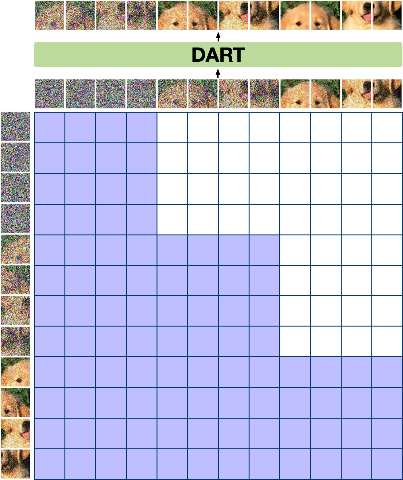
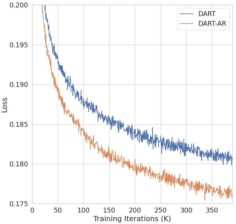
(a)	(b)	(c)

Figure 3: Attention masks for (a) DART and (b) DART-AR, highlighting their different structures. (c) Comparison of learning curves, demonstrating the superior performance of DART-AR.

3.2 Proposed Methods

Denoising AutoRegressive Transformer (DART)

We propose DART – a Transformer-based generative model that implements non-Markovian diffusion with an independent noising process (see Figure 2). First, following DiT (Peebles & Xie, 2022), we represent each image by first extracting the latent map with a pretrained VAE (Rombach et al., 2021), patchify, and flatten the map into a sequence of continuous tokens ${\bm{x}}_{t}\in\mathbb{R}^{K\times C}$, where $K$ is the length, and $C$ is the channel dimension. When considering multiple noise levels, we concat tokens along the length dimension. Then, DART models the generation as $p_{\theta}({\bm{x}}_{t-1}|{\bm{x}}_{t:T})=\mathcal{N}\left({\bm{x}}_{t-1};\sqrt{\gamma_{t-1}}{\bm{x}}_{\theta}({\bm{x}}_{t:T}),(1-\gamma_{t-1})\mathbf{I}\right)$, where ${\bm{x}}_{\theta}(.)$ is a Transformer network that takes in the concatenated sequence ${\bm{x}}_{t:T}\in\mathbb{R}^{K(T-t)\times C}$, and predicts the “mean” of the next noisy image. By combining with Eq 6, we simplify Eq 5 as:

$$\min\mathcal{L}^{\textrm{DART{}}}_{\theta}=\mathbb{E}_{{\bm{x}}_{1:T}\sim q({\bm{x}}_{0})}\left[\sum_{t=1}^{T}\omega_{t}\cdot\|{\bm{x}}_{\theta}({\bm{x}}_{t:T})-{\bm{x}}_{0}\|^{2}_{2}\right],$$ (7)

where we define $\omega_{t}=\frac{\gamma_{t-1}}{1-\gamma_{t-1}}\tilde{\omega}_{t}$ to simplify the notation. Similar to standard AR models, training of $T$ denoising steps is in parallel, where computations across different steps are shared. A chunk-based causal mask is used to maintain the autoregressive structure (see Figure 3(a)).

It is evident from Eq 7 that the objective is similar to the original diffusion objective (Eq 2), demonstrating that DART can be trained as robustly as standard diffusion models. Additionally, by leveraging the diffusion trajectory within an autoregressive framework, DART allows us to incorporate the proven design principles of large language models (Brown et al., 2020; Dubey et al., 2024). Furthermore, Proposition 1 indicates that we can select $\omega_{t}$ according to its associated diffusion process. For instance, with SNR weighting (Ho et al., 2020), $\omega_{t}$ can be defined as $\omega_{t}=\sum_{\tau=t}^{T}\frac{\gamma_{\tau}}{1-\gamma_{\tau}}$.

Sampling from DART is straightforward: we simply predict the mean ${\bm{x}}_{\theta}({\bm{x}}_{t:T})$, add Gaussian noise to obtain the next step $\hat{{\bm{x}}}_{t-1}$, and feed that to the following iteration. Unlike diffusion models, no complex solvers are needed. Similar to diffusion models, classifier-free guidance (CFG, Ho & Salimans, 2021) is applied to the prediction of ${\bm{x}}_{\theta}$ for improved visual quality. Additionally, KV-cache is employed to enhance decoding efficiency.

Limitations of Naive DART

Unlike diffusion models, which can be trained with a large number of steps $T$, non-Markovian modeling is constrained by memory consumption as $T$ increases. For example, using $T=16$ on $256\times 256$ images will easily create over $4000$ tokens even in the latent space. This fundamentally limits the modeling capacity on complex tasks such as text-to-image generation. However, the flexibility of the autoregressive structure allows us to enhance the capacity without compromising scalability. In this work, we propose two methods on top of DART:

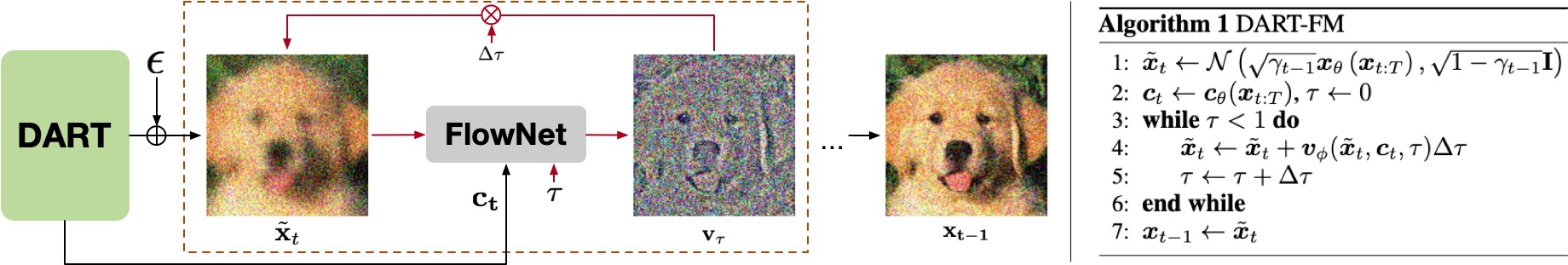
Figure 4: An illustration for the generation process of DART-FM.

1. DART with Token Autoregressive (DART-AR)

As similarly discussed by Xiao et al. (2021), the independent Gaussian assumption of $p_{\theta}({\bm{x}}_{t-1}|{\bm{x}}_{t:T})$ is inaccurate to approximate the complex true distribution of $q({\bm{x}}_{t-1}|{\bm{x}}_{t:T})$, especially when $T$ is small. A straightforward solution to model image denoising as an additional autoregressive model $p_{\theta}({\bm{x}}_{t-1}|{\bm{x}}_{t:T})=\prod_{k=1}^{K}p_{\theta}({\bm{x}}_{k,t-1}|{\bm{x}}_{<k,t-1},{\bm{x}}_{t:T})$:

$$\min\mathcal{L}^{\textrm{DART{}-AR}}_{\theta}=\mathbb{E}_{{\bm{x}}_{1:T}\sim q({\bm{x}}_{0})}\left[\sum_{t=1}^{T}\omega_{t}\sum_{k=1}^{K}\|{\bm{x}}_{\theta}({\bm{x}}_{<k,t-1},{\bm{x}}_{t:T})-{\bm{x}}_{k,0}\|^{2}_{2}\right],$$ (8)

where ${\bm{x}}_{1,t-1},\ldots,{\bm{x}}_{K,t-1}$ are the $K$ flatten tokens of ${\bm{x}}_{t-1}$. The autoregressive decomposition ensures each tokens are not independent, which is strictly stronger than the original DART. We demonstrate this by visualizing the training curve in Figure 3 (c). Training of DART-AR takes essentially the same amount of computation as standard DART with two additional modifications at the input and attention masks (see comparison in Figure 3 (a) (b)). At sampling time, DART-AR is relatively much more expensive as it requires $K\times T$ AR steps before it outputs the final prediction.

2. DART with Flow Matching (DART-FM)

The above approach models dependency across tokens, while maintaining Gaussian modeling at each step. Alternatively, we can improve the expressiveness of $p_{\theta}({\bm{x}}_{t-1}|{\bm{x}}_{t:T})$ by abandoning the Gaussian assumption, similar to Li et al. (2024). More precisely, we first sample $\tilde{{\bm{x}}}_{t}$ as in regular DART. Then, we recursively apply a continuous flow network, ${\bm{v}}_{\phi}(\tilde{{\bm{x}}}_{t},{\bm{c}}_{t},\tau_{t})$, over multiple iterations to bridge the gap between $\tilde{{\bm{x}}}_{t}$ and ${\bm{x}}_{t-1}$ (see Figure 4). Here, ${\bm{v}}_{\phi}(\tilde{{\bm{x}}}_{t},{\bm{c}}_{t},\tau)$ models the velocity field for the probabality flow between the distributions of $\tilde{{\bm{x}}}_{t}$ and ${\bm{x}}_{t-1}$, $\tau\in[0,1]$ denotes the auxiliary flow timestep, and ${\bm{c}}_{t}={\bm{c}}_{\theta}({\bm{x}}_{t:T})$ represents the features from the last Transformer block, providing contextual information across the noisy image. Consequently, a simple MLP suffices to model ${\bm{v}}_{\phi}$, adding only a minimal overhead to the total training cost. We train ${\bm{v}}_{\phi}$ via flow matching (Liu et al., 2022; Lipman et al., 2023; Albergo et al., 2023) due to its simplicity:

$$\min\mathcal{L}^{\textrm{FM}}_{\phi,\theta}=\mathbb{E}_{{\bm{x}}_{1:T}\sim q({\bm{x}}_{0})}\sum_{t=1}^{T}\mathbb{E}_{\tau\in[0,1]}\|{\bm{v}}_{\phi}((1-\tau)\tilde{{\bm{x}}}_{t}+\tau{\bm{x}}_{t-1},{\bm{c}}_{t},\tau)-({\bm{x}}_{t-1}-\tilde{{\bm{x}}}_{t})\|^{2}_{2},$$ (9)

where $\tilde{{\bm{x}}}_{t}=\sqrt{\gamma_{t-1}}\texttt{SG}\left[{\bm{x}}_{\theta}({\bm{x}}_{t:T})\right]+\sqrt{1-\gamma_{t-1}}\mathbf{\epsilon}$, and $\mathbf{\epsilon}\sim\mathcal{N}(0,\mathbf{I})$. $\texttt{SG}\left[\right]$ is the stop-gradient operator to avoid trivial solutions in optimization. In practice, we combine Eq 9 with the original DART objectives, which can be seen as an additional refinement on top of the Gaussian-based prediction.

3.3 Multi-resolution Generation

DART (including both the -AR and -FM variants) is a highly flexible framework that can be easily extended and applied in various scenarios with minimal changes in the formulation. For example, instead of learning a fixed resolution of images, one can learn a joint distribution of $p_{\theta}(\{{\bm{x}}^{i}_{0}\}_{i=1}^{N})$ where ${\bm{x}}^{i}_{0}\in\mathbb{R}^{K_{i}\times C}$ is ${\bm{x}}_{0}$ with a different resolution. Following the approaches proposed in Gu et al. (2022; 2023); Zheng et al. (2023) for diffusion models, a single DART — referred to as Matryoshka-DART — can model multiple resolutions by representing each image with its corresponding noisy sequence $\{{\bm{x}}^{k}_{t}\}_{t}$ separately, then flattening and concatenating these sequences for sequential prediction. As a special case shown in Figure 5 ($\leftarrow$), we model the NOMAD objective in Eq 5 as

$$\max\mathcal{L}^{\textrm{Matryoshka}}_{\theta}=\mathbb{E}_{\{\{{\bm{x}}^{i}_{t}\}_{t=0}^{T_{i}}\}_{i=1}^{N}\sim q({\bm{x}}_{0})}\left[\sum_{i=1}^{N}\sum_{t=1}^{T}\tilde{\omega}_{t}^{i}\cdot\log p_{\theta}({\bm{x}}_{t-1}^{i}|{\bm{x}}^{i}_{t:T},{\bm{x}}^{<i}_{1:T})\right],$$ (10)

where the above can be implemented using any DART variant. Note that ${\bm{x}}^{i}_{0}$ is not directly conditioned on ${\bm{x}}^{<i}_{0}$, which not only avoids the need to handle shape changes at the boundaries but also mitigates potential error propagation, a common issue in learning cascaded diffusion (Ho et al., 2022). All low-resolution information is processed through self-attention.

By this approach, the model can balance the number of noise levels with the total number of tokens to achieve better efficiency. Additionally, learning resolutions can be progressively increased by finetuning low-resolution models with extended sequences.

3.4 Multi-modal Generation

Our proposed framework, built on an autoregressive model, naturally extends to discrete token modeling tasks. This includes discrete latent modeling for image generation (Gu et al., 2024) and multi-modal generation (Team, 2024). By leveraging a shared architecture, we jointly optimize for both continuous denoising and next-token prediction loss using cross-entropy for discrete latents which we call Kaleido-DART considering its architectural similarity as Gu et al. (2024) (see Figure 5). To balance inference across modalities, we reweight the discrete loss (Eq 3) according to the relative lengths between the discrete and image tokens:

$$\mathcal{L}^{\textrm{Kaleido}}_{\theta}=\lambda\mathcal{L}^{\textrm{CE}}_{\theta}+\mathcal{L}^{\textrm{DART}}_{\theta},$$ (11)

where $\lambda=\frac{\textrm{\# text tokens}}{\textrm{\# image tokens}}$. It is important to note that our approach is markedly distinct from several concurrent works aimed at unifying autoregressive and diffusion models within a single parameter space (Zhou et al., 2024; Xie et al., 2024; Zhao et al., 2024; Xiao et al., 2024). In these efforts, the primary goal is to adapt language model architectures to perform diffusion tasks, without modifying the underlying diffusion process itself to account for the shift in model design. As we have discussed, the Markovian nature of diffusion models inherently limits their ability to leverage generation history, a feature that lies at the core of autoregressive models. In contrast, DART is designed to merge the advantages of both autoregressive and diffusion frameworks, fully exploiting the autoregressive capabilities. This formulation also allows for seamless integration into LLM pipelines.

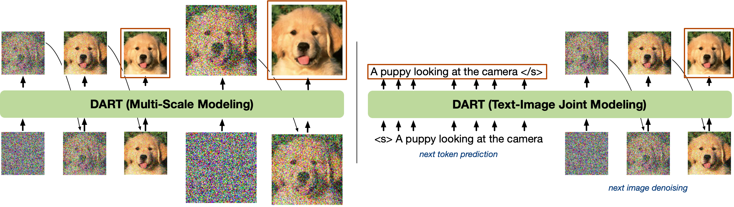
Figure 5: Illustrations of Matryoshka-DART ($\leftarrow$) and Kaleido-DART ($\rightarrow$). By joint training models, DART can perform various applications such as multi-resolution and multi-modal generation.

4 Experiments

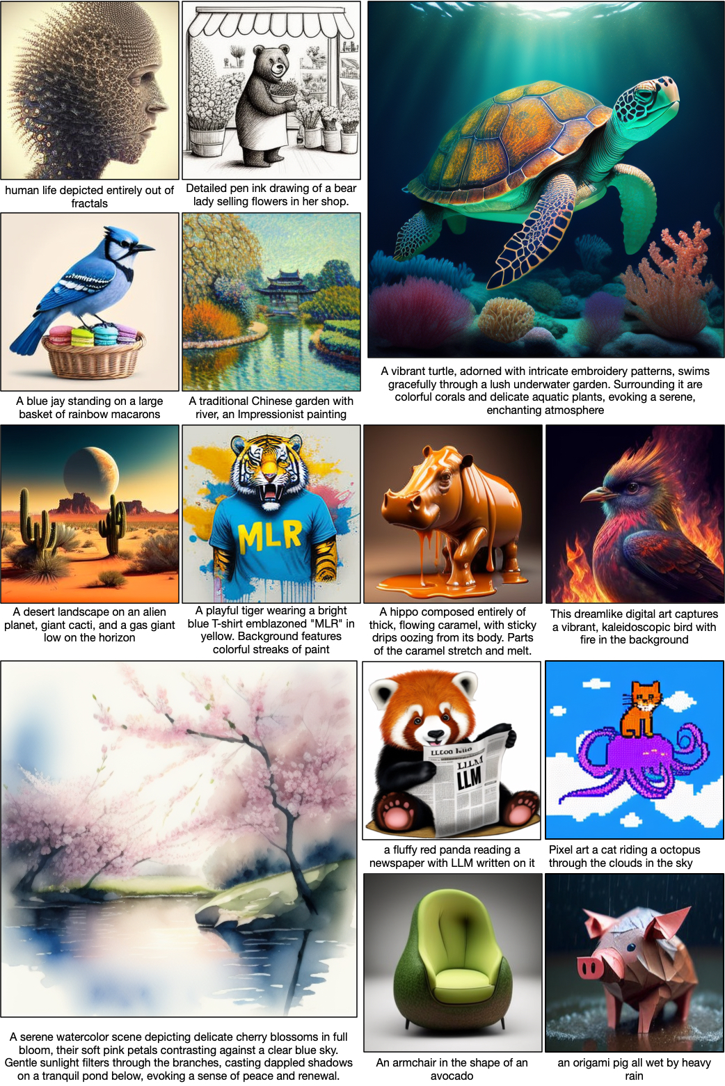
Figure 6: Samples generated by text-to-image DART-FM at $256\times 256$ and $512\times 152$ pixels

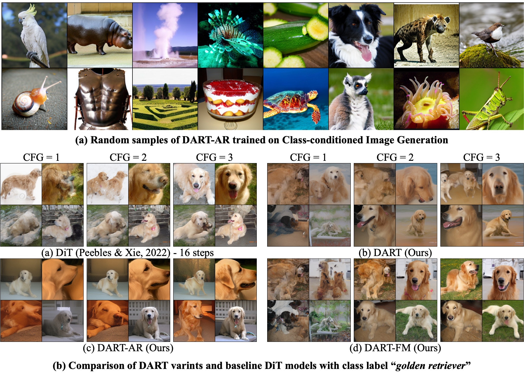
Figure 7: Comparison for class-conditioned image generation with DART and baselines trained on ImageNet.

4.1 Experimental Settings

Dataset

We experiment with DART on both class-conditioned image generation on ImageNet (Deng et al., 2009) and text-to-image generation on CC12M (Changpinyo et al., 2021), where each image is accompanied by a descriptive caption. All images are center-cropped and resized. All models, except those used for Matryoshka-DART finetuning, are trained to synthesize images at $256\times 256$ resolution, while the latter are trained at $512\times 512$. For multimodal generation tasks, we augment CC12M with synthetic captions as the discrete ground-truth.

Evaluation

In line with prior works, we report Fréchet Inception Distance (FID) (Heusel et al., 2017) to quantify the the realism and diversity of generated images. For text-to-image generation, we also use the CLIP score (Hessel et al., 2021) to measure how well the generated images align with the given text instructions. To assess the zero-shot capabilities of the models, we report scores based on the MSCOCO 2017 (Lin et al., 2014) validation set.

Architecture

Following § 3.2, we experimented with three variants of the proposed model: the default DART, along with two enhanced versions, DART-AR and DART-FM. All variants are implemented using the same Transformer blocks for consistency. As illustrated in Figure 2, our design is similar to Dubey et al. (2024), incorporating rotary positional encodings (RoPE, Su et al., 2024) within the self-attention layers and SwiGLU activation (Shazeer, 2020) in the FFN layers. For class-conditioned generation, we follow (Peebles & Xie, 2022), adding an AdaLN block to each Transformer block to integrate class-label information. For text-to-image generation, we replace AdaLN with additional cross-attention layers over pretrained T5-XL encoder (Raffel et al., 2020). Since DART uses a fixed noise schedule, there is no need for extra time embeddings as long as RoPE is active. In addition, for DART-FM, we incorporate a small flow network, implemented as a 3-layer MLP, which increases the total parameter count by only about 1%.

Training & Inference

Proposition 1 not only makes a connection between DART and diffusion models, but also allows us to define the noise schedule based on any existing diffusion schedule $\{\bar{\alpha}_{t}\}_{t}$, which can be inversely mapped to the DART schedule $\{\gamma_{t}\}_{t}$ using the bijection. In this paper, we adopt the cosine schedule $\bar{\alpha}_{t}=\cos{\left({\pi}/{2}\cdot{t}/{T}\right)}$. We set $T=16$ while $K=256$ throughout all experiments unless otherwise specified. We train all models with a batch size of 128 images, resulting in a total of 0.5M image tokens per update. For finetuning Matryoshka-DART, we additionally set the high-resolution part $T=4$ with $K=1024$. We use the AdamW optimizer (Loshchilov & Hutter, 2017) with a cosine learning rate schedule, setting the maximum learning rate to $3\textrm{e-}4$. During inference, we enable KV-cache with memory pre-allocated based on the total sequence length. DART performs the same number of steps for inference as in training. For the FM variants, we additionally apply $100$ flow matching steps between each autoregressive step, following Li et al. (2024). More implementation details can be found in Appendix B.

4.2 Results

Class-conditioned Generation

We report the FID scores for conditional ImageNet generation in Figure 8(a), following the approach of previous works. In line with Li et al. (2024), we apply a linear CFG scheduler to DART and its variants. As shown in the figure, both -AR and -FM variants consistently outperform the default DART across all guidance scales, demonstrating the effectiveness of the proposed improvement strategies. We also compare our methods with DiT (Peebles & Xie, 2022), using both 16 sampling steps (to match DART) and 250 steps (the suggested best setting). Notably, DART-AR achieves the best FID score of 3.98 among all variants and significantly surpasses DiT when using 16 steps, highlighting its advantage in leveraging generative trajectories, particularly when the number of sampling timesteps is limited. Not surprisingly, DiT with 250 steps performs better than DART. However, it is important to note that the official DiT model is trained for 7M steps, which is substantially more training iterations than those used for DART.

Figure 7 also presents examples of generated results on ImageNet from all models using 16 sampling steps. DART-FM tends to produce sharper images with higher fidelity at higher CFG values. In contrast, DART-AR demonstrates an ability to generate more realistic samples at lower CFG values when compared to both the baselines and other variants. More samples are shown in Appendix C.

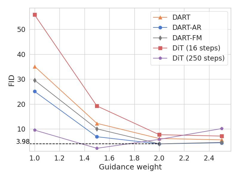
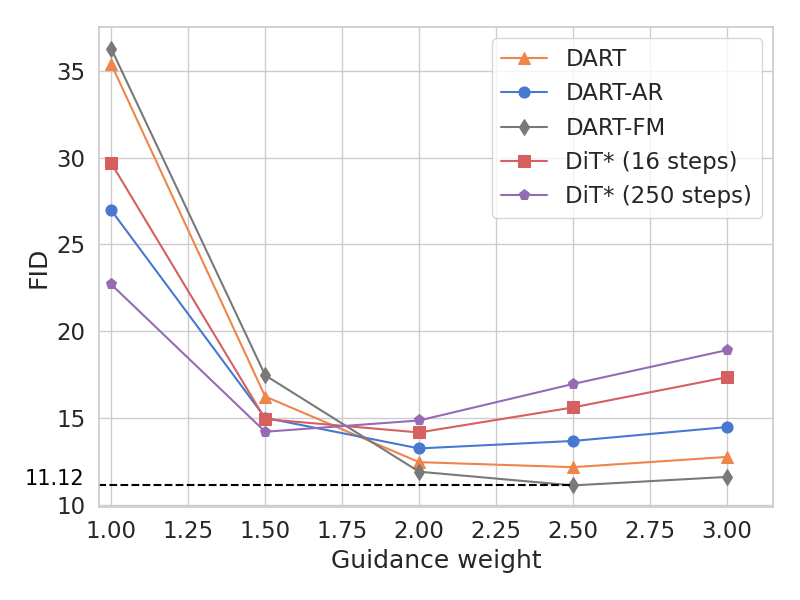
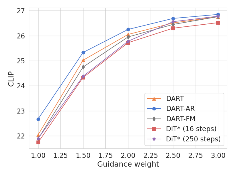
(a) FID50K on ImageNet	(b) FID30K on COCO	(c) CLIP score on COCO

Figure 8: Comparison of DART, DART-AR, DART-FM and baseline models with different CFG guidance scale on different benchmarks. * denotes models implemented and trained by us.

Model Gflops Speed (s) DART 2.157 0.075 DART-AR 2.112 7.44 DART-FM 2.177 0.32 DiT (16) 2.073 0.065 DiT (256) 32.384 0.84
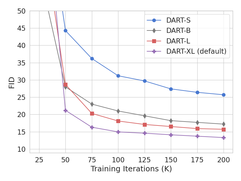
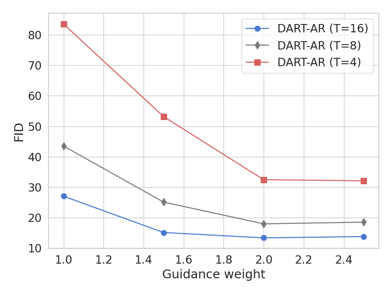
(a) Inference speed & flops	(b) Comparison of model sizes	(c) Comparison of # of steps

Figure 9: (a) Inference flops and speed (caulated as second per image) of different models. (b) Performance of DART of different sizes. (c) Effect of number of noise levels on DART.

Text-to-Image Generation

To demonstrate the capability of DART at scale, we train the model for text-to-image generation. We also implement an in-house DiT with cross attention to text condition in comparison to our models, where we evaluate the performance on both $16$ and $250$ steps. As shown in Figure 8, while both -AR and -FM variants still show clear improvements against the default DART, FM achieves the best FID of 11.12, indicating its ability of handling diverse generation tasks.

To validate the scalability of high-resolution image generation, we further finetune DART by jointly modeling $256\times 256$ and $512\times 512$ resolutions within a single autoregressive process (§ 3.3). Sampled results are shown in Figure 6 and Appendix C.

Efficiency

We compare both the actual inference speed (measured by wall-clock time with batch size 32 on a single H100) as well as the theoretical computation (measured by GFlops) in 9(a). Since DART, DART-AR, DART-FM share the same encoder-decoder Transformer architecture, their flops are roughly the same. However, DART-AR has high wall clock inference time due to its large autoregressive steps, which have not been well parallelized in our current implementation. Integrated with recent advances in autoregressive LLMs, DART-AR can be deployed in a more efficient and we leave this for future investigations. DART-FM also have a inference time overhead due to the iterations of flow net in inference. Compared to DART, DiT has less flops for a single pass. However, it requires sufficient many number of iterations to generate high quality samples. DART has comparable flops and inference time as DiT with 16 sampling timesteps, while DART achieves better performance than DiT (16) on ImageNet and COCO, showing the efficiency benefits of DART.

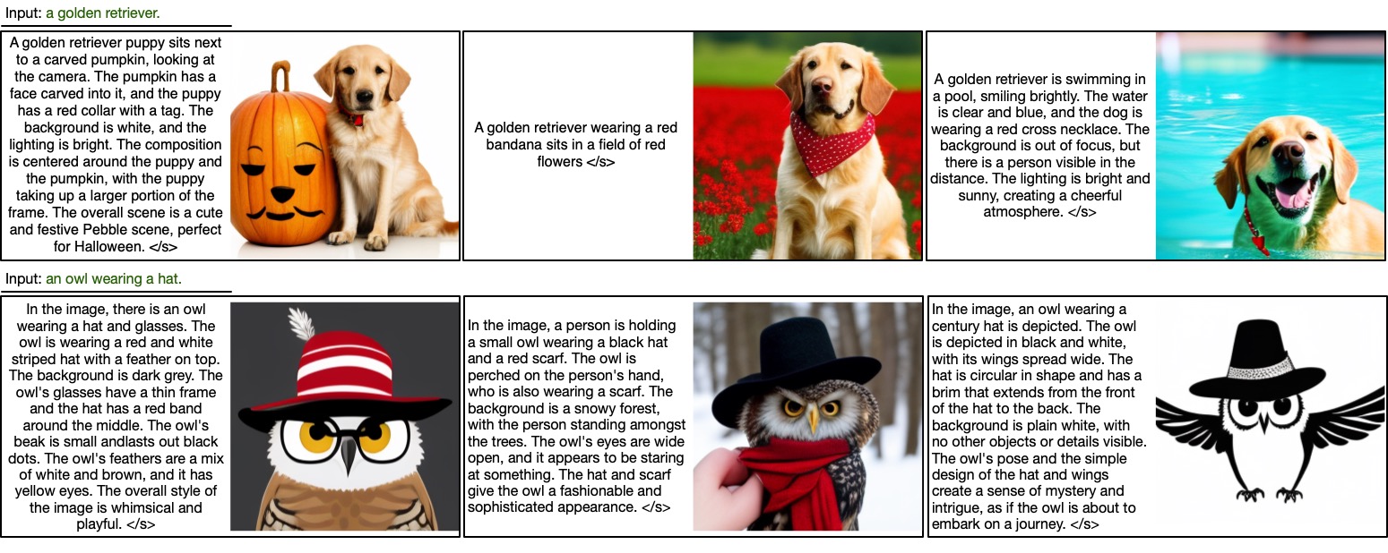
Figure 10: Examples of multi-modal generation with Kaleido-DART.

Scalibility

We show the scalability of our DART by training models of different sizes including small (S), base (B), large (L), and extra large (XL) on CC12M, where the configurations are listed in Appendix B.1. Figure 9(b) illustrates how the performance changes as model size increase. Across all the four models, CLIP score significantly improves by increasing the number of parameters in DART. Besides, the perform steadily increases as more training iterations are applied. This demonstrates that our proposed generative paradigm benefits from scaling as previous generative models like diffusion (Peebles & Xie, 2022) and autoregressive models (Li et al., 2024).

Effects of noise levels.

We experiment with different noise levels, where we vary the number of total noise levels in our denoising framework (Figure 9(c)). A total of $T=4$ or $8$ noise levels are trained in comparison with standard $16$ noise levels. Not surprisingly, less noise levels lead to gradually degraded performance. However, with as few as 4 noise levels, DART can still generate plausible samples, indicating the capabilities of deploying DART in a more efficient way. Variants in noise levels provides a potential option for finding the optimal computation and performance trade-off especially when compute is limited.

Multimodal Generation

We showcase the capabilities of our proposed method in the joint generation of discrete text and continuous images, as introduced in § 3.4. Figure 10 provides examples of multimodal generation using the Kaleido-DART framework. Given an input, the model generates rich descriptive texts along with corresponding realistic images, demonstrating its ability to produce diverse samples with intricate details. Notably, unlike Gu et al. (2024), our approach processes both text and images through the same model, utilizing a unified mechanism to handle both modalities. This unified framework can potentially be integrated into any multimodal language models.

5 Conclusion

We presented DART, a novel model that integrates autoregressive denoising with non-Markovian diffusion to improve the efficiency and scalability of image generation. By leveraging the full generation trajectory and incorporating token-level autoregression and flow matching, DART achieves competitive performance on class-conditioned and text-to-image tasks. This approach offers a unified and flexible solution for high-quality visual synthesis.

Our current model is restricted by the number of tokens in the denoising process. One direction is to explore more efficient architectures for long context modeling (Gu & Dao, 2023; Yan et al., 2024) which enables application to problems like video generations. Also, current work only conduct preliminary investigates on multimodal generation. Future work may train a multimodal generative model based on the framework of the decoder-only language model to handle a wide variety of problems with one unified model.

Appendix A Proof of Proposition 1

Proof.

Due to $q({\bm{x}}_{t}|{\bm{x}}_{0})=\mathcal{N}({\bm{x}}_{t};\sqrt{\gamma_{t}}{\bm{x}}_{0},(1-\gamma_{t})\mathbf{I})$, we can write ${\bm{x}}_{t}=\sqrt{\gamma_{t}}{\bm{x}}_{0}+\sqrt{1-\gamma_{t}}{\bm{\epsilon}}_{t}$.

With certain coefficient $\{\lambda^{t}_{s}\}_{s=t}^{T}$, let us define:

$${\bm{y}}_{t} \triangleq\sum_{s=t}^{T}\lambda^{t}_{s}{\bm{x}}_{s},$$ (12)

We study when the signal-to-noise ratio of ${\bm{y}}_{t}$ achieves its maximal value:

$${\bm{y}}_{t} =\left(\sum_{s=t}^{T}\lambda^{t}_{s}\sqrt{\gamma_{s}}\right){\bm{x}}_{0}+\sum_{s=t}^{T}\lambda^{t}_{s}\sqrt{1-\gamma_{s}}{\bm{\epsilon}}_{s}$$ (13)

$$\Rightarrow\text{SNR}({\bm{y}}_{t}) =\frac{\left(\sum_{s=t}^{T}\lambda^{t}_{s}\sqrt{\gamma_{s}}\right)^{2}}{\sum_{s=t}^{T}{\lambda^{t}_{s}}^{2}(1-\gamma_{s})}\leq\sum_{s=t}^{T}\frac{\gamma_{s}}{1-\gamma_{s}},$$ (14)

which follows from Titu’s lemma and the Cauchy-Schwarz inequality. It becomes an equality when:

$$\lambda^{t}_{s}\propto\frac{\sqrt{\gamma_{s}}}{1-\gamma_{s}},\forall s\in[t,T]$$ (15)

Next, we demonstrate that $\{{\bm{y}}_{t}\}_{t}$ follows a Markov property when achieving the maximal signal-to-noise ratio for each ${\bm{y}}_{t}$. From Eq 15, let $\lambda_{s}^{t}=\rho_{t}\frac{\sqrt{\gamma_{s}}}{1-\gamma_{s}},\rho_{t}>0$, and $\eta_{t}=\frac{\gamma_{t}}{1-\gamma_{t}}$, $\bar{\eta}_{t}=\sum_{s=t}^{T}\eta_{s}$, we have:

$${\bm{y}}_{t} =\rho_{t}\left(\bar{\eta}_{t}{\bm{x}}_{0}+\sum_{s=t}^{T}\sqrt{\eta_{s}}{\bm{\epsilon}}_{s}\right)$$ (16)

$$=\rho_{t}\left(\bar{\eta}_{t}{\bm{x}}_{0}+\sqrt{\bar{\eta}_{t}}{\bm{\epsilon}}^{\prime}_{t}\right),$$ (17)

where we use ${\bm{\epsilon}}^{\prime}_{t}\sim\mathcal{N}(0,\mathbf{I})$ to equivalently simplify the noise term. When $\rho_{t}=1\big{/}\sqrt{\bar{\eta}^{2}_{t}+\bar{\eta}_{t}}$, $\{{\bm{y}}_{t}\}_{t}$ is variance preserving (VP). Next, let us assume

$$\hat{{\bm{y}}} =\frac{\rho_{t+1}\bar{\eta}_{t+1}}{\rho_{t}\bar{\eta}_{t}}{\bm{y}}_{t}+\sigma{\bm{\epsilon}},{\bm{\epsilon}}\sim\mathcal{N}(0,\mathbf{I})$$ (18)

$$=\rho_{t+1}\bar{\eta}_{t+1}{\bm{x}}_{0}+\rho_{t+1}\bar{\eta}_{t+1}/\sqrt{\bar{\eta}}_{t}{\bm{\epsilon}}^{\prime}_{t}+\sigma{\bm{\epsilon}}$$ (19)

$$=\rho_{t+1}\left(\bar{\eta}_{t+1}{\bm{x}}_{0}+\sqrt{\frac{\bar{\eta}_{t+1}^{2}}{\bar{\eta}_{t}}+\frac{\sigma^{2}}{\rho^{2}_{t+1}}}{\bm{\epsilon}}^{\prime\prime}\right),$$ (20)

where we use ${\bm{\epsilon}}^{\prime\prime}$ to replace the noise term. So if we let $\hat{{\bm{y}}}$ match the distribution of ${\bm{y}}_{t+1}$, then

$$\frac{\bar{\eta}_{t+1}^{2}}{\bar{\eta}_{t}}+\frac{\sigma^{2}}{\rho^{2}_{t+1}}=\bar{\eta}_{t+1}$$ (21)

$$\Rightarrow\;\; \sigma^{2}=\rho^{2}_{t+1}\frac{\bar{\eta}_{t+1}\eta_{t}}{\bar{\eta}_{t}}>0$$ (22)

The above equation has root that $\sigma=\rho_{t+1}\sqrt{{\bar{\eta}_{t+1}\eta_{t}}\big{/}{\bar{\eta}_{t}}}$, This implies that we can find an independent noise term added to ${\bm{y}}_{t}$ to obtain ${\bm{y}}_{t+1}$, establishing that ${{\bm{y}}_{t}}_{t}$ constitutes a Markovian forward process.

$$p({\bm{y}}_{t+1}|{\bm{y}}_{t})=\mathcal{N}\left(\frac{\rho_{t+1}\bar{\eta}_{t+1}}{\rho_{t}\bar{\eta}_{t}}{\bm{y}}_{t},\rho^{2}_{t+1}{\frac{\bar{\eta}_{t+1}\eta_{t}}{\bar{\eta}_{t}}\mathbf{I}}\right)$$ (23)

What’s more, $\{{\bm{x}}_{t}\}_{t}$ sequence can be uniquely determined from $\{{\bm{y}}_{t}\}_{t}$ via

$${\bm{x}}_{t}=\begin{cases}\left(\dfrac{{\bm{y}}_{t}}{\rho_{t}}-\dfrac{{\bm{y}}_{t+1}}{\rho_{t+1}}\right)\dfrac{1-\gamma_{t}}{\sqrt{\gamma}_{t}},&\text{if }t<T\\ \dfrac{{\bm{y}}_{t}}{\rho_{t}}\dfrac{1-\gamma_{t}}{\sqrt{\gamma}_{t}},&\text{if }t=T.\end{cases}$$ (24)

Therefore, the two processes $\{{\bm{x}}_{t}\}_{t}$ and $\{{\bm{y}}_{t}\}_{t}$ has a one-to-one correspondence.

∎

Appendix B Implementation Details

B.1 Architecture

In this paper, we use encoder-decoder Transformer architecture (Vaswani et al., 2017a) to implement our DART model. The total number of parameters in our standard model is about 800M. For text-to-image (T2I) generation, we employ pretrained Flan-T5-XL (Raffel et al., 2020; Chung et al., 2022) as the textual encoder in all experiments. During training, the encoder is frozen and only the decoder is trained. For class-conditioned (C2I) generation, the encoder is simply a embedding layer, mapping a class label into a fixed length vector. Since we do not use a text encoder for cross-attention, we pass context information through Adaptive LayerNorm. To maintain parity in the total number of parameters with text-to-image models, we set the hidden size to $1152$. Below is the default configurations of DARTs.

model config for DARTs:
    patch_size=2
    hidden_size=1280 (T2I) or 1152 (C2I)
    num_layers=28
    num_channels_per_head=64
    use_swiglu_ffn=True
    use_rope=True
    rope_axes_dim=[16,24,24]
    use_per_head_rmsnorm=True
    use_adaln=False (T2I) or True (C2I)
    lm_feature_projected_channels=2048

Table 1 lists the configurations of different model sizes used in the scalability experiments of §4.2. For DART-FM, we implement the flow network as three MLPs (FFNs) with additional adaptive LayerNorm for modulation. Unlike standard FFN blocks in Transformers, the hidden size in our implementation remains unchanged, matching the hidden dimension of the main DART blocks.

Table 1: Configurations of DART of different sizes.

Model	# Layers	Hidden size	# Heads	# Params
DART-S	12	384	6	48M
DART-B	12	768	12	141M
DART-L	24	1024	16	464M
DART-XL	28	1280	20	812M

In Matryoshka-DART upsample tuning, we follow the default setting and set the patch size as 2 for $512\times 512$ images, which end up containing 1024 tokens each. In total, the model has 8192 tokens in total, including 4096 tokens for $256\times 256$ images with 16 denoising steps and 4096 tokens for $512\times 512$ images with 4 denoising steps. We also applies rotary positional embedding (RoPE) (Su et al., 2024) to embed the information of token position. We find it critical to spatially align the positional embedding of high resolution images with low resolution ones. In particular, we define the rotary matrix feature at position $(i,j)$ in a $256\times 256$ image as $\mathbf{R}_{\Theta}^{(i,j)}$. For feature $x^{(i^{\prime},j^{\prime})}$ at position $(i^{\prime},j^{\prime})$ in the corresponding high resolution image with upsample ratio $r$, the rotary matrix is given $\mathbf{R}_{\Theta}^{(i^{\prime}/r,j^{\prime}/r)}$. In our case, the ratio is 2, which halves the position values on $512\times 512$ images.

B.2 Training

In all the experiments, we share the following training configuration for our proposed DART.

default training config:
    batch_size=128
    optimizer=’AdamW’
    adam_beta1=0.9
    adam_beta2=0.95
    adam_eps=1e-8
    learning_rate=3e-4
    warmup_steps=10_000
    weight_decay=0.01
    gradient_clip_norm=2.0
    ema_decay=0.9999
    mixed_precision_training=bf16

B.3 Parameterization of Diffusion Model

In our implementation, we employ v-prediction (Salimans & Ho, 2022) for improved performance. Namely, DART is trained to output ${\bm{v}}_{t}=\frac{\alpha_{t}{\bm{x}}_{t}-{\bm{x}}}{\sigma_{t}}$. The prediction of the model $\tilde{{\bm{v}}}_{t}$ is mapped to the clean image through $\tilde{{\bm{x}}}=\alpha_{t}{\bm{x}}_{t}-\sigma_{t}\tilde{{\bm{v}}}_{t}$. The loss is then computed between ${\bm{x}}$ and $\tilde{{\bm{x}}}$, and the loss weighting is also applied here.

Appendix C Additional Samples

C.1 Prompts for Figure 1 (from left to right, top to bottom)

• Cinematic photo of a fluffy baby Quokka with a knitted hat eating a large cup of popcorns, close up, studio lighting, screen reflecting in its eyes. 35mm photographs, film, bokeh, professional, 4k, highly detailed

• A golden autumn scene, with the sun shining through a canopy of orange and red leaves, a path covered in fallen leaves, and soft light casting long shadows

• Detailed pen and ink drawing of the arrival of a giant alien ship.

• A diffusion cloud expanding in a cosmic scene, with the words ’DART’ subtly emerging from the nebula, blending into the stars and dust

• A polar bear made entirely of vanilla ice cream, standing on a waffle cone iceberg with chocolate syrup dripping from its fur.

• A lion made entirely out of swirling fire, standing majestically on a rocky outcrop as the sun sets behind it.

• A pig made out of vegetables

• At a futuristic wedding ceremony, a robot sharp and precise, holds the hand of the other robot.

• A panda chef in a professional kitchen, wearing a chef’s hat and apron, carefully preparing a gourmet dish on the counter with steam rising from the pot.

• In the image, a corgi dog is wearing a Santa hat and is laying on a fluffy rug. The dog’s tongue is sticking out and it appears to be happy. There are two Christmas boxes and a basket of toys nearby, indicating that the scene takes place during the winter season. The background features a Christmas tree, further suggesting the holiday atmosphere. The image has a warm and cozy feel to it, with the dog looking adorable in its hat and the boxes adding a festive touch

• An astronaut standing on a frozen alien planet, looking up at a sky filled with two suns and a swirling aurora, with ice-covered

• A lighthouse standing tall on a rocky shore, with massive waves crashing against the base, as the beam of light cuts through the night.

• A scarecrow standing at the edge of a forest in early winter, its clothes dusted with fresh snow, with crows circling above against a cold, gray sky

• The phrase ’GenAI’ made of scattered coffee beans that form the letters, arranged on top of a white kitchen table with a coffee mug.

• An origami dragon made from rainbow-colored paper, soaring through a sky filled with clouds, leaving a trail of vibrant color behind it

• Photography closeup portrait of an adorable rusty broken down steampunk robot covered in budding vegetation, surrounded by tall grass, misty futuristic sci-fi forest environment

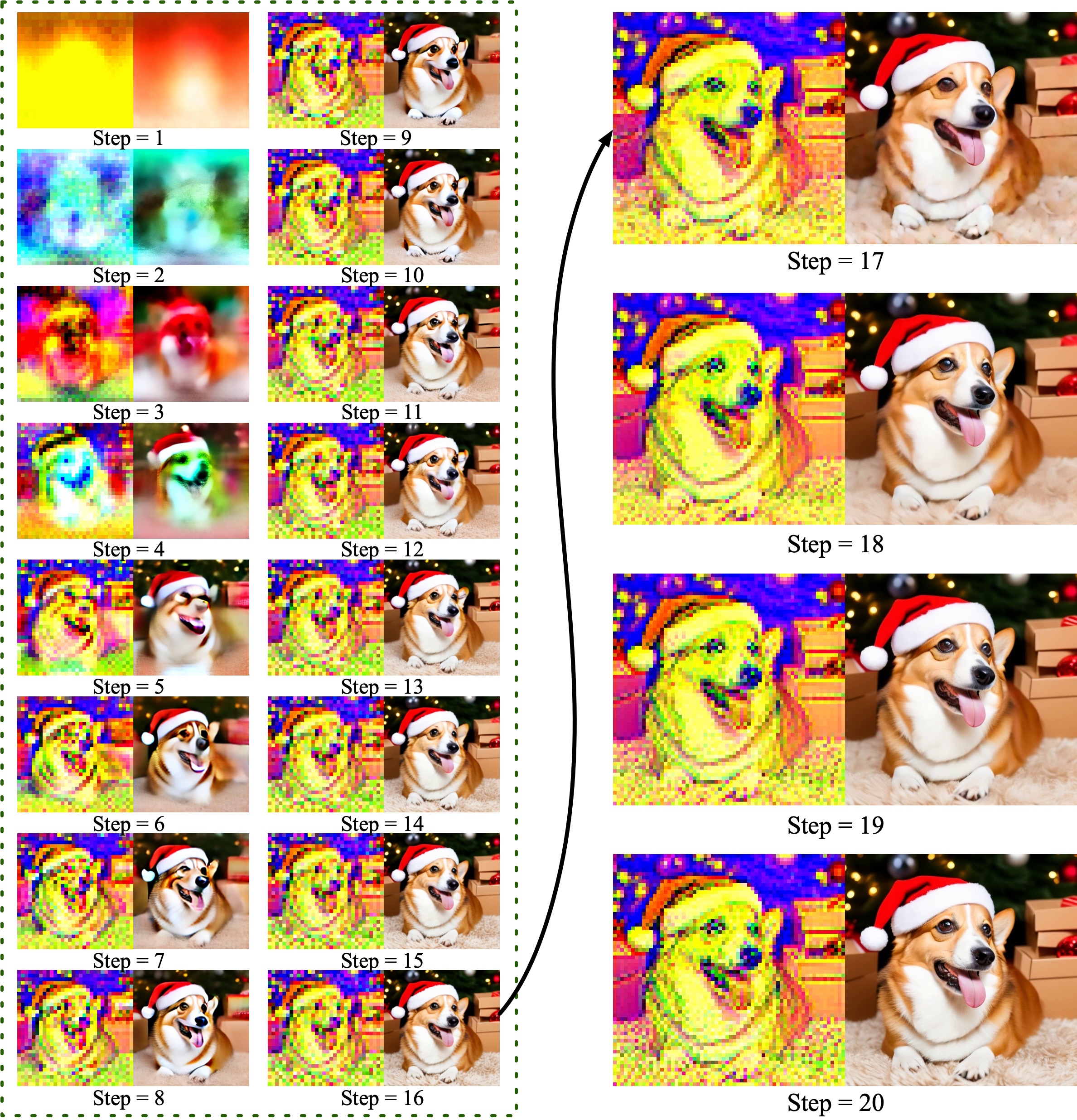
Figure 11: Visualization of the generation process (left: latent maps, right: decoded RGB images) for $256\times 256$ $(T=16)$ and its upsampling to $512\times 512$ $(T=4)$ using Matryoshka-DART.

C.2 Step-wise Generative Results

Figure 11 visualizes the generative process of an image at resolution $256\times 256$ and its upsampling to $512\times 512$ by Matryoshka-DART. DART first iteratively refines the generative results for 16 denoising steps at resolution $256\times 256$. It then upsamples images at resolution $512\times 512$ through iterative denoising as well. Since the generation of high resolution is conditioned on the previous low-resolution samples, it only needs 4 denoising steps at high resolution to generate realistic images.

C.3 Additional Samples

ImageNet

We here show more generative examples from DART variants trained on ImageNet $256\times 256$ in Figure 12. The proposed two improvement methods, DART-AR and DART-FM, generate images with higher fidelity and more details when compared with origin DART.

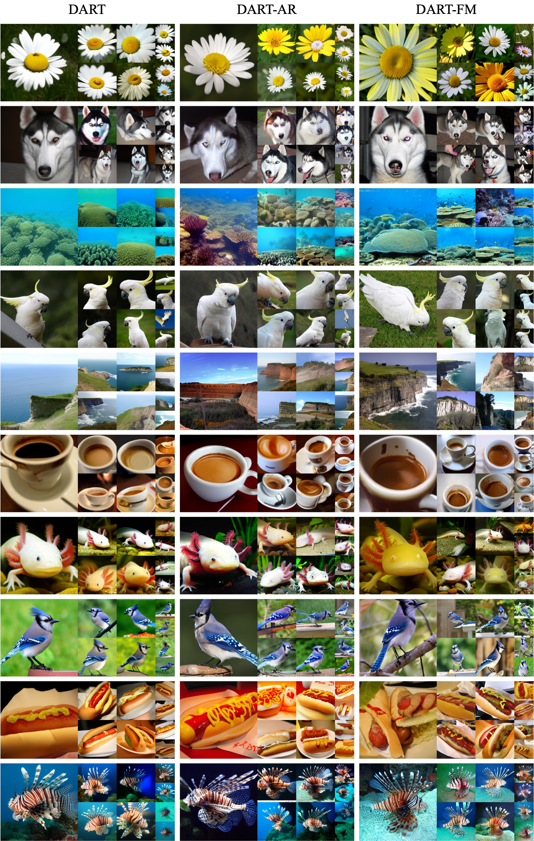
Figure 12: Uncurated samples from DART varints on ImageNet $256\times 256$ with for labels of daisy, husky, coral reel, sulphur-crested cockatoo, cliff, espresso, axolotl, jay, hotdog, lionfish.

Text-to-Image

We here show more text-to-image generative examples from DART-AR and DART-FM at resolution $256\times 256$ in Figure 13. We also show examples at resolution $512\times 512$ from Matryoshka-DART finetuned from DART-FM at $256\times 256$ in Figures 14 and 15.

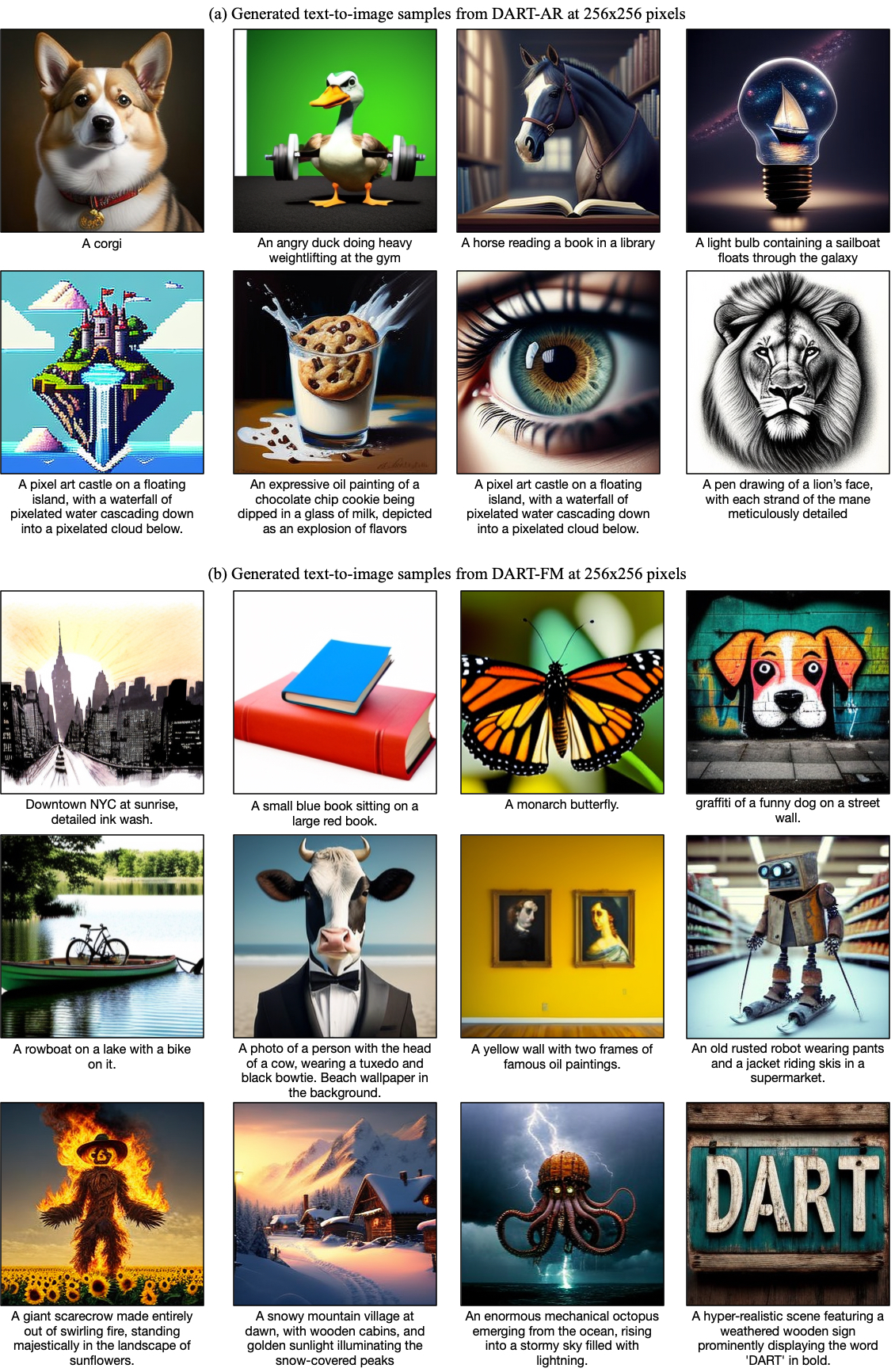
Figure 13: Uncurated samples from DART varints on text-to-image generation at $256\times 256$ pixels given various captions.

Figure 14: Uncurated samples from DART-FM with Matryoshka-DART fine-tuning on text-to-image generation at $512\times 512$ pixels given various captions.

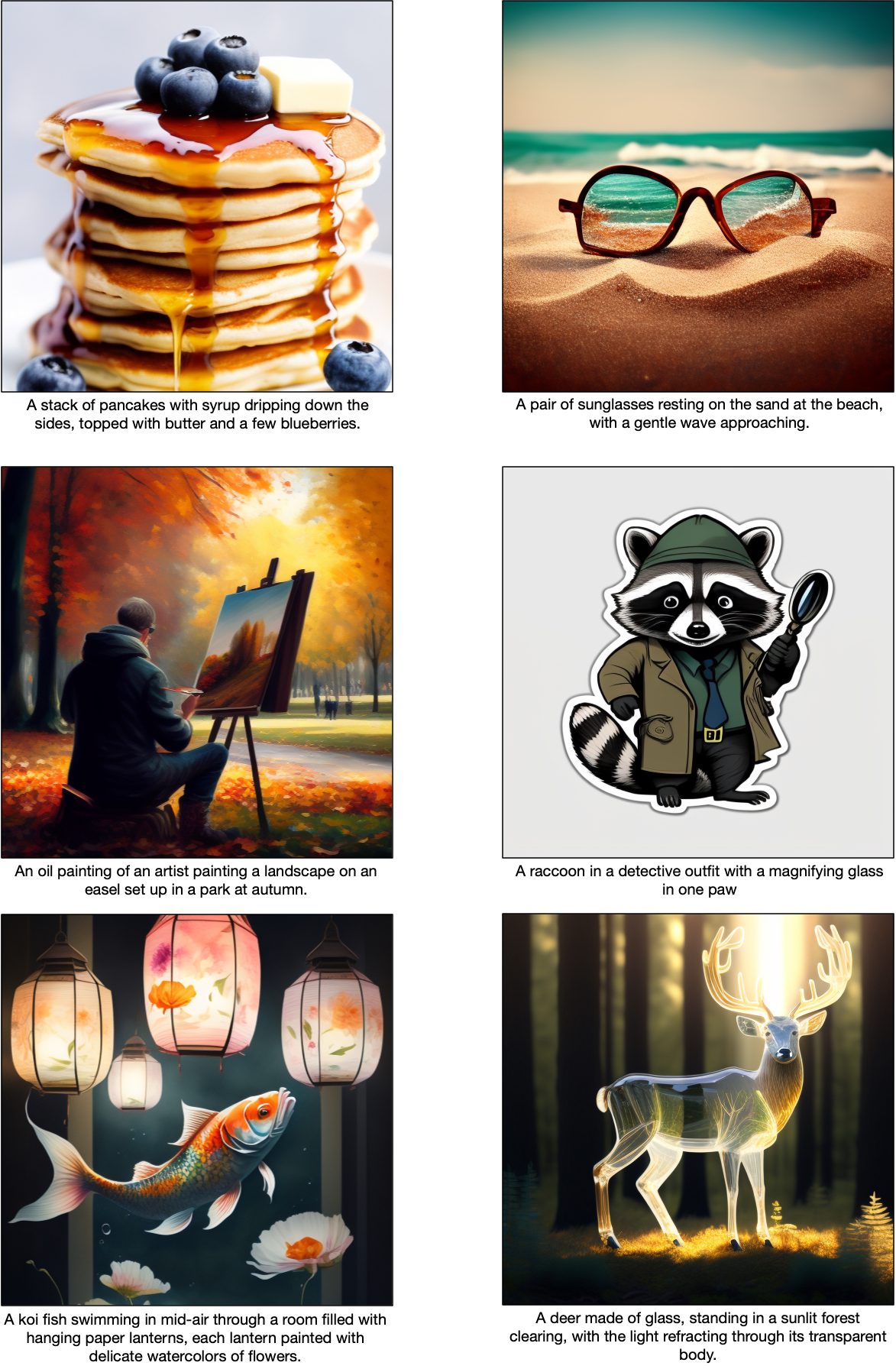
Figure 15: Uncurated samples from DART-FM with Matryoshka-DART fine-tuning on text-to-image generation at $512\times 512$ pixels given various captions.

References

- Achiam et al. (2023) Josh Achiam, Steven Adler, Sandhini Agarwal, Lama Ahmad, Ilge Akkaya, Florencia Leoni Aleman, Diogo Almeida, Janko Altenschmidt, Sam Altman, Shyamal Anadkat, et al. Gpt-4 technical report. arXiv preprint arXiv:2303.08774, 2023.
- Albergo et al. (2023) Michael S Albergo, Nicholas M Boffi, and Eric Vanden-Eijnden. Stochastic interpolants: A unifying framework for flows and diffusions. arXiv preprint arXiv:2303.08797, 2023.
- Brown et al. (2020) Tom B. Brown, Benjamin Mann, Nick Ryder, Melanie Subbiah, Jared Kaplan, Prafulla Dhariwal, Arvind Neelakantan, Pranav Shyam, Girish Sastry, Amanda Askell, Sandhini Agarwal, Ariel Herbert-Voss, Gretchen Krueger, Tom Henighan, Rewon Child, Aditya Ramesh, Daniel M. Ziegler, Jeffrey Wu, Clemens Winter, Christopher Hesse, Mark Chen, Eric Sigler, Mateusz Litwin, Scott Gray, Benjamin Chess, Jack Clark, Christopher Berner, Sam McCandlish, Alec Radford, Ilya Sutskever, and Dario Amodei. Language models are few-shot learners. Advances in neural information processing systems, 2020.
- Changpinyo et al. (2021) Soravit Changpinyo, Piyush Sharma, Nan Ding, and Radu Soricut. Conceptual 12M: Pushing web-scale image-text pre-training to recognize long-tail visual concepts. In CVPR, 2021.
- Chen et al. (2020) Mark Chen, Alec Radford, Rewon Child, Jeffrey Wu, Heewoo Jun, David Luan, and Ilya Sutskever. Generative pretraining from pixels. In International conference on machine learning, pp. 1691–1703. PMLR, 2020.
- Child (2021) Rewon Child. Very deep vaes generalize autoregressive models and can outperform them on images. In International Conference on Learning Representations, 2021.
- Chung et al. (2022) Hyung Won Chung, Le Hou, Shayne Longpre, Barret Zoph, Yi Tay, William Fedus, Eric Li, Xuezhi Wang, Mostafa Dehghani, Siddhartha Brahma, Albert Webson, Shixiang Shane Gu, Zhuyun Dai, Mirac Suzgun, Xinyun Chen, Aakanksha Chowdhery, Sharan Narang, Gaurav Mishra, Adams Yu, Vincent Zhao, Yanping Huang, Andrew Dai, Hongkun Yu, Slav Petrov, Ed H. Chi, Jeff Dean, Jacob Devlin, Adam Roberts, Denny Zhou, Quoc V. Le, and Jason Wei. Scaling instruction-finetuned language models, 2022. URL https://arxiv.org/abs/2210.11416.
- Deng et al. (2009) Jia Deng, Wei Dong, Richard Socher, Li-Jia Li, Kai Li, and Li Fei-Fei. ImageNet: A Large-scale Hierarchical Image Database. IEEE Conference on Computer Vision and Pattern Recognition, pp. 248–255, 2009.
- Dubey et al. (2024) Abhimanyu Dubey, Abhinav Jauhri, Abhinav Pandey, Abhishek Kadian, Ahmad Al-Dahle, Aiesha Letman, Akhil Mathur, Alan Schelten, Amy Yang, Angela Fan, et al. The llama 3 herd of models. arXiv preprint arXiv:2407.21783, 2024.
- Esser et al. (2021) Patrick Esser, Robin Rombach, and Bjorn Ommer. Taming transformers for high-resolution image synthesis. In Proceedings of the IEEE/CVF conference on computer vision and pattern recognition, pp. 12873–12883, 2021.
- Esser et al. (2024) Patrick Esser, Sumith Kulal, Andreas Blattmann, Rahim Entezari, Jonas Müller, Harry Saini, Yam Levi, Dominik Lorenz, Axel Sauer, Frederic Boesel, et al. Scaling rectified flow transformers for high-resolution image synthesis. In Forty-first International Conference on Machine Learning, 2024.
- Gu & Dao (2023) Albert Gu and Tri Dao. Mamba: Linear-time sequence modeling with selective state spaces. arXiv preprint arXiv:2312.00752, 2023.
- Gu et al. (2022) Jiatao Gu, Shuangfei Zhai, Yizhe Zhang, Miguel Angel Bautista, and Josh Susskind. f-dm: A multi-stage diffusion model via progressive signal transformation. arXiv preprint arXiv:2210.04955, 2022.
- Gu et al. (2023) Jiatao Gu, Shuangfei Zhai, Yizhe Zhang, Joshua M Susskind, and Navdeep Jaitly. Matryoshka diffusion models. In The Twelfth International Conference on Learning Representations, 2023.
- Gu et al. (2024) Jiatao Gu, Ying Shen, Shuangfei Zhai, Yizhe Zhang, Navdeep Jaitly, and Joshua M Susskind. Kaleido diffusion: Improving conditional diffusion models with autoregressive latent modeling. arXiv preprint arXiv:2405.21048, 2024.
- Hessel et al. (2021) Jack Hessel, Ari Holtzman, Maxwell Forbes, Ronan Le Bras, and Yejin Choi. Clipscore: A reference-free evaluation metric for image captioning. In Proceedings of the 2021 Conference on Empirical Methods in Natural Language Processing, pp. 7514–7528, 2021.
- Heusel et al. (2017) Martin Heusel, Hubert Ramsauer, Thomas Unterthiner, Bernhard Nessler, and Sepp Hochreiter. Gans trained by a two time-scale update rule converge to a local nash equilibrium. Advances in neural information processing systems, 30, 2017.
- Ho & Salimans (2021) Jonathan Ho and Tim Salimans. Classifier-free diffusion guidance. In NeurIPS 2021 Workshop on Deep Generative Models and Downstream Applications, 2021.
- Ho et al. (2020) Jonathan Ho, Ajay Jain, and Pieter Abbeel. Denoising diffusion probabilistic models. Advances in Neural Information Processing Systems, 33:6840–6851, 2020.
- Ho et al. (2022) Jonathan Ho, Chitwan Saharia, William Chan, David J Fleet, Mohammad Norouzi, and Tim Salimans. Cascaded diffusion models for high fidelity image generation. J. Mach. Learn. Res., 23:47–1, 2022.
- Kilian et al. (2024) Maciej Kilian, Varun Japan, and Luke Zettlemoyer. Computational tradeoffs in image synthesis: Diffusion, masked-token, and next-token prediction. arXiv preprint arXiv:2405.13218, 2024.
- Kingma et al. (2021) Diederik Kingma, Tim Salimans, Ben Poole, and Jonathan Ho. Variational diffusion models. Advances in neural information processing systems, 34:21696–21707, 2021.
- Kingma & Welling (2013) Diederik P Kingma and Max Welling. Auto-encoding variational bayes. arXiv preprint arXiv:1312.6114, 2013.
- Li et al. (2024) Tianhong Li, Yonglong Tian, He Li, Mingyang Deng, and Kaiming He. Autoregressive image generation without vector quantization. arXiv preprint arXiv:2406.11838, 2024.
- Lin et al. (2014) Tsung-Yi Lin, Michael Maire, Serge Belongie, James Hays, Pietro Perona, Deva Ramanan, Piotr Dollár, and C. Lawrence Zitnick. Microsoft COCO: Common Objects in Context. European Conference on Computer Vision, pp. 740–755, 2014.
- Lipman et al. (2023) Yaron Lipman, Ricky T. Q. Chen, Heli Ben-Hamu, Maximilian Nickel, and Matthew Le. Flow matching for generative modeling. In The Eleventh International Conference on Learning Representations, 2023. URL https://openreview.net/forum?id=PqvMRDCJT9t.
- Liu et al. (2022) Xingchao Liu, Chengyue Gong, and Qiang Liu. Flow straight and fast: Learning to generate and transfer data with rectified flow. arXiv preprint arXiv:2209.03003, 2022.
- Loshchilov & Hutter (2017) Ilya Loshchilov and Frank Hutter. Decoupled weight decay regularization. arXiv preprint arXiv:1711.05101, 2017.
- Oord et al. (2016) Aaron van den Oord, Nal Kalchbrenner, and Koray Kavukcuoglu. Pixel Recurrent Neural Networks. ICML, 2016.
- Parmar et al. (2018) Niki Parmar, Ashish Vaswani, Jakob Uszkoreit, Lukasz Kaiser, Noam Shazeer, Alexander Ku, and Dustin Tran. Image transformer. In International conference on machine learning, pp. 4055–4064. PMLR, 2018.
- Peebles & Xie (2022) William Peebles and Saining Xie. Scalable diffusion models with transformers. arXiv preprint arXiv:2212.09748, 2022.
- Podell et al. (2023) Dustin Podell, Zion English, Kyle Lacey, Andreas Blattmann, Tim Dockhorn, Jonas Müller, Joe Penna, and Robin Rombach. Sdxl: improving latent diffusion models for high-resolution image synthesis. arXiv preprint arXiv:2307.01952, 2023.
- Raffel et al. (2020) Colin Raffel, Noam Shazeer, Adam Roberts, Katherine Lee, Sharan Narang, Michael Matena, Yanqi Zhou, Wei Li, and Peter J Liu. Exploring the limits of transfer learning with a unified text-to-text transformer. Journal of machine learning research, 21(140):1–67, 2020.
- Rombach et al. (2021) Robin Rombach, Andreas Blattmann, Dominik Lorenz, Patrick Esser, and Björn Ommer. High-resolution image synthesis with latent diffusion models, 2021.
- Rombach et al. (2022) Robin Rombach, Andreas Blattmann, Dominik Lorenz, Patrick Esser, and Björn Ommer. High-resolution image synthesis with latent diffusion models. In Proceedings of the IEEE/CVF conference on computer vision and pattern recognition, pp. 10684–10695, 2022.
- Saharia et al. (2022) Chitwan Saharia, William Chan, Saurabh Saxena, Lala Li, Jay Whang, Emily L Denton, Kamyar Ghasemipour, Raphael Gontijo Lopes, Burcu Karagol Ayan, Tim Salimans, et al. Photorealistic text-to-image diffusion models with deep language understanding. Advances in Neural Information Processing Systems, 35:36479–36494, 2022.
- Salimans & Ho (2022) Tim Salimans and Jonathan Ho. Progressive distillation for fast sampling of diffusion models. arXiv preprint arXiv:2202.00512, 2022.
- Shazeer (2020) Noam Shazeer. Glu variants improve transformer. arXiv preprint arXiv:2002.05202, 2020.
- Sohl-Dickstein et al. (2015) Jascha Sohl-Dickstein, Eric Weiss, Niru Maheswaranathan, and Surya Ganguli. Deep unsupervised learning using nonequilibrium thermodynamics. In International Conference on Machine Learning, pp. 2256–2265. PMLR, 2015.
- Song et al. (2021) Jiaming Song, Chenlin Meng, and Stefano Ermon. Denoising diffusion implicit models. In International Conference on Learning Representations, 2021.
- Song et al. (2020) Yang Song, Jascha Sohl-Dickstein, Diederik P Kingma, Abhishek Kumar, Stefano Ermon, and Ben Poole. Score-based generative modeling through stochastic differential equations. arXiv preprint arXiv:2011.13456, 2020.
- Su et al. (2024) Jianlin Su, Murtadha Ahmed, Yu Lu, Shengfeng Pan, Wen Bo, and Yunfeng Liu. Roformer: Enhanced transformer with rotary position embedding. Neurocomputing, 568:127063, 2024.
- Sun et al. (2024) Peize Sun, Yi Jiang, Shoufa Chen, Shilong Zhang, Bingyue Peng, Ping Luo, and Zehuan Yuan. Autoregressive model beats diffusion: Llama for scalable image generation. arXiv preprint arXiv:2406.06525, 2024.
- Team (2024) Chameleon Team. Chameleon: Mixed-modal early-fusion foundation models. arXiv preprint arXiv:2405.09818, 2024.
- Tian et al. (2024) Keyu Tian, Yi Jiang, Zehuan Yuan, Bingyue Peng, and Liwei Wang. Visual autoregressive modeling: Scalable image generation via next-scale prediction. arXiv preprint arXiv:2404.02905, 2024.
- Van Den Oord et al. (2017) Aaron Van Den Oord, Oriol Vinyals, et al. Neural discrete representation learning. Advances in neural information processing systems, 30, 2017.
- Vaswani et al. (2017a) Ashish Vaswani, Noam Shazeer, Niki Parmar, Jakob Uszkoreit, Llion Jones, Aidan N. Gomez, Lukasz Kaiser, and Illia Polosukhin. Attention Is All You Need. Advances in Neural Information Processing Systems, pp. 5998–6008, 2017a.
- Vaswani et al. (2017b) Ashish Vaswani, Noam Shazeer, Niki Parmar, Jakob Uszkoreit, Llion Jones, Aidan N Gomez, Łukasz Kaiser, and Illia Polosukhin. Attention is all you need. In Advances in neural information processing systems, pp. 5998–6008, 2017b.
- Xiao et al. (2024) Shitao Xiao, Yueze Wang, Junjie Zhou, Huaying Yuan, Xingrun Xing, Ruiran Yan, Shuting Wang, Tiejun Huang, and Zheng Liu. Omnigen: Unified image generation. arXiv preprint arXiv:2409.11340, 2024.
- Xiao et al. (2021) Zhisheng Xiao, Karsten Kreis, and Arash Vahdat. Tackling the generative learning trilemma with denoising diffusion gans. arXiv preprint arXiv:2112.07804, 2021.
- Xie et al. (2024) Jinheng Xie, Weijia Mao, Zechen Bai, David Junhao Zhang, Weihao Wang, Kevin Qinghong Lin, Yuchao Gu, Zhijie Chen, Zhenheng Yang, and Mike Zheng Shou. Show-o: One single transformer to unify multimodal understanding and generation. arXiv preprint arXiv:2408.12528, 2024.
- Yan et al. (2024) Jing Nathan Yan, Jiatao Gu, and Alexander M Rush. Diffusion models without attention. In Proceedings of the IEEE/CVF Conference on Computer Vision and Pattern Recognition, pp. 8239–8249, 2024.
- Yu et al. (2022) Jiahui Yu, Yuanzhong Xu, Jing Yu Koh, Thang Luong, Gunjan Baid, Zirui Wang, Vijay Vasudevan, Alexander Ku, Yinfei Yang, Burcu Karagol Ayan, et al. Scaling autoregressive models for content-rich text-to-image generation. Transactions on Machine Learning Research, 2022.
- Zhao et al. (2024) Chuyang Zhao, Yuxing Song, Wenhao Wang, Haocheng Feng, Errui Ding, Yifan Sun, Xinyan Xiao, and Jingdong Wang. Monoformer: One transformer for both diffusion and autoregression. arXiv preprint arXiv:2409.16280, 2024.
- Zheng et al. (2023) Huangjie Zheng, Zhendong Wang, Jianbo Yuan, Guanghan Ning, Pengcheng He, Quanzeng You, Hongxia Yang, and Mingyuan Zhou. Learning stackable and skippable lego bricks for efficient, reconfigurable, and variable-resolution diffusion modeling. In The Twelfth International Conference on Learning Representations, 2023.
- Zhou et al. (2024) Chunting Zhou, Lili Yu, Arun Babu, Kushal Tirumala, Michihiro Yasunaga, Leonid Shamis, Jacob Kahn, Xuezhe Ma, Luke Zettlemoyer, and Omer Levy. Transfusion: Predict the next token and diffuse images with one multi-modal model. arXiv preprint arXiv:2408.11039, 2024.