On Densest $k$-Subgraph Mining and Diagonal Loading

Abstract

The Densest $k$-Subgraph (D$k$S) problem aims to find a subgraph comprising $k$ vertices with the maximum number of edges between them. A continuous reformulation of the binary quadratic D$k$S problem is considered, which incorporates a diagonal loading term. It is shown that this non-convex, continuous relaxation is tight for a range of diagonal loading parameters, and the impact of the diagonal loading parameter on the optimization landscape is studied. On the algorithmic side, two projection-free algorithms are proposed to tackle the relaxed problem, based on Frank-Wolfe and explicit constraint parametrization, respectively. Experiments suggest that both algorithms have merits relative to the state-of-art, while the Frank-Wolfe-based algorithm stands out in terms of subgraph density, computational complexity, and ability to scale up to very large datasets.

1 Introduction

Dense subgraph detection (DSD) aims to extract highly interconnected subsets of vertices from a graph. DSD is a key primitive in graph mining (see the surveys [1, 2] and references therein), and finds application in diverse settings ranging from discovering DNA motifs [3] to mining trending topics in social media [4] and discovering complex patterns in gene annotation graphs [5]. In recent years, DSD has also been employed for detecting fraudulent activities occurring in e-commerce and financial transaction networks [6, 7, 8, 9].

Owing to its relevance, the development of algorithmic approaches for DSD has received extensive attention. A widely-used formulation for DSD is the Densest Subgraph (DSG) problem [10], which aims to extract the subgraph with the maximum average induced degree. DSG can be solved exactly in polynomial time via maximum-flow, while a lower complexity alternative is a greedy peeling algorithm that runs in linear time and provides a $1/2$-factor approximation guarantee [11]. Recent work [12, 13] has developed multi-stage extensions of the basic greedy algorithm, which provide improved approximation guarantees for DSG at roughly the same complexity. Another popular approach for DSD is to compute the $k$-core of a graph [14], which corresponds to the subgraph that maximizes the minimum induced degree. The greedy algorithm for DSG (with a slight tweak) optimally computes the $k$-core in linear-time. Recently, Veldt et al. [15] provided a more general framework for computing solutions of degree-based density objectives, which contain DSG and $k$-core as special cases.

An inherent limitation of the aforementioned approaches is that the size of the extracted subgraph cannot be explicitly controlled, which raises the possibility that the solution may be a large subgraph that is too sparsely connected to be practically useful. These observations have been made on real-world graphs for DSG [16] and the $k$-core [17]. A natural remedy is to add an explicit size constraint to DSG, leading to the Densest $k$-Subgraph (D$k$S) problem [18]. The objective of D$k$S is to find a size-$k$ vertex subset with the maximum average induced degree. By varying the size parameter $k$, D$k$S can extract a spectrum of dense subgraphs, providing flexibility for users to select a solution with the desired density when the outputs of the aforementioned approaches are unsatisfactory. However, this simple modification makes the resulting D$k$S problem NP-hard. Furthermore, D$k$S has been shown to be difficult to approximate [19, 20] in the worst case. Hence, developing effective algorithmic tools for D$k$S (on practical instances) is substantially more challenging compared to DSG or $k$-core extraction. It is also worth noting that there are variants of D$k$S that impose size constraints on the extracted subgraph [21, 22, 23]. However, using these formulations does not guarantee that the entire spectrum of densest subgraphs (i.e., of every size) can be explored.

1.1 Related Work

The best polynomial-time approximation algorithm for D$k$S can provide an $O(n^{1/4+\epsilon})$-approximation solution in time $O(n^{1/\epsilon})$ for every $\epsilon>0$ [24], which is generally quite pessimistic. Bhaskara et al. [25] proposed using a hierarchy of linear programming (LP) relaxations of increasing complexity to approximate D$k$S, which makes it unattractive for large datasets. Even implementing the lowest level of the hierarchy is computationally expensive, as a large number of extra variables and linear inequalities have to be introduced in order to successfully linearize the quadratic objective function of D$k$S. Meanwhile, Ames [26] formulated D$k$S as a rank-constrained optimization problem, which was then relaxed and solved using the Alternating Direction Method of Multipliers (ADMM) [27]. However, implementing the approach requires using matrix lifting, which results in a quadratic number of variables and thus makes it unsuitable for even moderately sized problem instances. A different relaxation of D$k$S which uses semi-definite programming (SDP) was proposed by Bombina and Ames in [28]. The relaxation provides optimality guarantees for D$k$S when applied on a certain class of random graphs. In addition to the high complexity entailed in solving the SDP, the optimality claims of the proposed algorithm in [28] do not extend straightforwardly to real-world graphs. Barman [29] reformulated D$k$S as the Normalized Densest $k$-Subgraph problem (ND$k$S) and proved that an $\epsilon$-additive approximate solution of ND$k$S can be found in polynomial time if an $\epsilon$-additive approximate solution of a specific continuous relaxation of ND$k$S is given. However, no practical numerical algorithm was given in [29].

Since the aforementioned algorithms are sophisticated and can incur high computational complexity, efforts have also focused on developing more practical algorithms for the D$k$S problem. Yuan and Zhang [30] proposed using the Truncated Power Method (TPM) for tackling D$k$S and proved the convergence of this algorithm under certain conditions. However, in practice, the subgraphs obtained by TPM can be highly sub-optimal. Papailiopoulos et al. [31] employed the Spannogram, an exact solver for certain low-rank bilinear optimization problems, to approximately solve the D$k$S problem. If the graph adjacency matrix has a constant rank, it was shown that the Spannogram can approximate the solution to the D$k$S problem in polynomial time. Improving the approximation quality may require choosing a relatively high rank, which limits scalability due to the exponential dependence of the algorithm’s time complexity on the rank. Even performing a rank-2 approximation using the Spannogram framework incurs $O(n^{3})$ complexity, making it challenging to apply to large-scale problems.

A separate line of research has considered applying continuous relaxations of D$k$S followed by application of gradient-based optimization algorithms. Hager et al. [32] introduced a relaxation of D$k$S and applied a pair of gradient-based optimization algorithms for solving it. A different relaxation was introduced by Sotirov in [33], and coordinate descent algorithms were applied to solve it. However, neither [32] nor [33] analyzed whether the relaxations are tight or not. In [34], an alternate convex relaxation was proposed by Konar and Sidiropoulos which is based on using the Lovaśz extension of the objective function of D$k$S as a convex surrogate. A customized algorithm based on an inexact version of ADMM [35] was put forth to solve the relaxed formulation. Nonetheless, [34] also did not provide an analysis of whether the relaxation is tight and the computational cost of the proposed algorithm can also be relatively high. Recently, Liu et al. [36] introduced Extreme Point Pursuit (EXPP), which relaxes the discrete constraint of D$k$S, and adopts a quadratic penalty based approach combined with a homotopy optimization technique to tackle the relaxed problem. They employed an empirical strategy for selecting the penalty parameter for homotopy optimization, and it remains unclear whether their relaxation is tight.

1.2 Contributions

Our contributions can be summarized as follows:

• We adopt a continuous relaxation of the D$k$S problem with diagonal loading. Although the resulting problem is non-convex, we establish the minimum value of the diagonal loading parameter $\lambda$ to ensure that the relaxation is tight. We derive the lower bound and the upper bound of this result via a non-trivial extension of the classic Motzkin-Straus theorem [37] and an extension of Lemma 5.1 in [29]. Furthermore, our result reveals that the value of $\lambda$ required to establish tightness of the diagonal loading based relaxation is much smaller than that obtained using classical results in optimization [38]. The upshot is that the optimization landscape of such a “lightly” loaded relaxation can be more amenable to gradient-based optimization approaches.

• To efficiently obtain (approximate) solutions of the relaxed optimization problem, we utilize two iterative gradient-based approaches: one based on the Frank-Wolfe algorithm [39, 40] and the other based on explicit constraint parameterization. A key feature of these methods is that they are projection-free, meaning they avoid the need to compute computationally expensive projections onto the constraint set of the proposed relaxation, which enhances their scalability. We provide a complexity analysis demonstrating that the computational cost of the proposed parameterization approach is not prohibitive, while that of the Frank-Wolfe approach is surprisingly low.

• We validate the effectiveness of diagonal loading empirically and demonstrate that the proposed algorithms, especially the Frank-Wolfe algorithm, achieve state-of-the-art results across several real-world datasets. We also show that the Frank-Wolfe algorithm achieves good subgraph density while maintaining low computational complexity.

It is important to point out that the Frank-Wolfe framework has been previously applied for solving DSG in [41]. However, the application is on a formulation which is very different from our considered relaxation (see problem (5) in section “Problem Formulation”). Perhaps the most important difference is that the problem considered in [41] is convex, whereas problem (5) is not. Hence, the Frank-Wolfe algorithm applied to (5) (see Algorithm $1$) has different properties in terms of convergence, step size selection, and implementation.

1.3 Notation

In this paper, lowercase regular font is used to represent scalars, lowercase bold font is used to represent vectors, uppercase bold font is used to represent matrices, calligraphic font is used to represent sets or pairs of sets. $x_{i}$ denotes the $i$-the element of the vector $\boldsymbol{x}$. $\boldsymbol{x}^{(t)}$ and $a^{(t)}$ denote the scalar $a$ and the vector $\boldsymbol{x}$ at the $t$-th iteration, respectively. $[n]$ denotes the set $\{1,2,\dots,n\}$. $(\cdot)^{\mathsf{T}}$ denotes the transpose of a vector or a matrix. $\boldsymbol{A}\succeq\boldsymbol{0}$ denotes $\boldsymbol{A}$ is a positive semi-definite matrix. $\|\cdot\|_{2}$ denotes the Euclidean norm of a vector or the spectral norm of a matrix. $|\cdot|$ denotes the cardinality of a set. $\text{top}_{k}(\boldsymbol{x})$ denotes the index set of the largest $k$ elements in $\boldsymbol{x}$. $\boldsymbol{x}[\mathcal{C}]\leftarrow a$ denotes assigning the value $a$ to the entries of $\boldsymbol{x}$ corresponding to $\mathcal{C}$.

2 Problem Formulation

Consider an unweighted, undirected, and simple graph $\mathcal{G}=(\mathcal{V},\mathcal{E})$ with $n$ vertices and $m$ edges, where $\mathcal{V}=\{1,\dots,n\}$ represents the vertex set and $\mathcal{E}$ is the edge set. Given a positive integer $k\in[n]$, the D$k$S problem aims to find a vertex subset $\mathcal{S}\subseteq\mathcal{V}$ of size $k$ such that the subgraph induced by $\mathcal{S}$ has the maximum average degree. Formally, the problem can be expressed as

$$\max_{\boldsymbol{x}\in\mathbb{R}^{n}} f(\boldsymbol{x})=\boldsymbol{x}^{\mathsf{T}}\boldsymbol{A}\boldsymbol{x}$$ (1)

s.t. $$\boldsymbol{x}\in\mathcal{B}_{k}^{n},$$

where $\boldsymbol{A}$ is the symmetric $n\times n$ adjacency matrix of $\mathcal{G}$ and the constraint set $\mathcal{B}_{k}^{n}=\{\boldsymbol{x}\in\mathbb{R}^{n}|\boldsymbol{x}\in\{0,1\}^{n},\sum_{i\in[n]}x_{i}=k\}$ captures the subgraph size restriction. The binary vector $\boldsymbol{x}\in\{0,1\}^{n}$ is an indicator vector corresponding to the selected vertices in the subset $\mathcal{S}$, i.e.,

$$x_{i}=\begin{cases}1,&\text{if }i\in\mathcal{S},\\ 0,&\text{otherwise}.\end{cases}$$ (2)

The combinatorial sum-to-$k$ constraint in (1) makes the D$k$S problem hard to solve. A natural choice to alleviate the difficulty is to relax the constraint to its convex hull, a strategy also employed in [33, 34, 36]. After relaxation, the problem can be formulated as

$$\max_{\boldsymbol{x}\in\mathbb{R}^{n}} f(\boldsymbol{x})=\boldsymbol{x}^{\mathsf{T}}\boldsymbol{A}\boldsymbol{x}$$ (3)

s.t. $$\boldsymbol{x}\in\mathcal{C}_{k}^{n},$$

where $\mathcal{C}_{k}^{n}=\{\boldsymbol{x}\in\mathbb{R}^{n}|\boldsymbol{x}\in[0,1]^{n},\sum_{i\in[n]}x_{i}=k\}$ is a polytope that represents the convex hull of $\mathcal{B}_{k}^{n}$. As the problem is now continuous, it is amenable to (approximate) maximization via gradient-based methods. However, we cannot guarantee that the optimal solution of (1) remains optimal for (3), indicating that the relaxation from (1) to (3) might not be tight. One way to address this issue is to introduce a regularization term in the objective function to promote sparsity in the solution. This can be achieved by equivalently reformulating (1) as

$$\max_{\boldsymbol{x}\in\mathbb{R}^{n}} g(\boldsymbol{x})=\boldsymbol{x}^{\mathsf{T}}(\boldsymbol{A}+\lambda\boldsymbol{I})\boldsymbol{x}$$ (4)

s.t. $$\boldsymbol{x}\in\mathcal{B}_{k}^{n},$$

where $\lambda$ is a non-negative constant and $\boldsymbol{I}$ is the identity matrix of size $n$. We refer to this trick as “diagonal loading” with parameter $\lambda$. Similar to the relaxation from (1) to (3), the combinatorial constraint $\mathcal{B}_{k}^{n}$ in (4) can be relaxed to $\mathcal{C}_{k}^{n}$, yielding the following relaxation

$$\max_{\boldsymbol{x}\in\mathbb{R}^{n}} g(\boldsymbol{x})=\boldsymbol{x}^{\mathsf{T}}(\boldsymbol{A}+\lambda\boldsymbol{I})\boldsymbol{x}$$ (5)

s.t. $$\boldsymbol{x}\in\mathcal{C}_{k}^{n}.$$

If $\lambda$ is selected large enough so that the matrix $\boldsymbol{A}+\lambda\boldsymbol{I}\succeq\boldsymbol{0}$, (i.e., $\lambda\geq-\lambda_{n}(\boldsymbol{A})$, where $\lambda_{n}(\boldsymbol{A})$ denotes the smallest eigenvalue of $\boldsymbol{A}$), then the objective function of (5) becomes convex. Since the maximum of a convex function over a polytope is attained at one of its extreme points, directly invoking [38, Theorem 32.2] shows that

$$\arg\max_{\boldsymbol{x}\in\mathcal{B}_{k}^{n}}\boldsymbol{x}^{\mathsf{T}}(\boldsymbol{A}+\lambda I)\boldsymbol{x}\subseteq\arg\max_{\boldsymbol{x}\in\mathcal{C}_{k}^{n}}\boldsymbol{x}^{\mathsf{T}}(\boldsymbol{A}+\lambda\boldsymbol{I})\boldsymbol{x}.$$ (6)

This implies that the maximum of $\boldsymbol{x}^{\mathsf{T}}(\boldsymbol{A}+\lambda\boldsymbol{I})\boldsymbol{x}$ over the combinatorial sum-to-$k$ constraint $\boldsymbol{x}\in\mathcal{B}_{k}^{n}$ (i.e., the solution of D$k$S) is attained only when $\boldsymbol{x}$ is also the maximum of $\boldsymbol{x}^{\mathsf{T}}(\boldsymbol{A}+\lambda\boldsymbol{I})\boldsymbol{x}$ over the continuous sum-to-$k$ constraint $\boldsymbol{x}\in\mathcal{C}_{k}^{n}$. In this paper, we say a relaxation is tight if every optimal solution of the original problem is also an optimal solution of the relaxed problem. It is also clear that if the relaxation from (4) to (5) is tight when the diagonal loading parameter $\lambda=\lambda^{\ast}$, then when the diagonal loading parameter $\lambda>\lambda^{\ast}$, the sets of optimal solutions of (4) and (5) are the same. Hence, for such a choice of $\lambda\geq-\lambda_{n}(\boldsymbol{A})$, the relaxation from (4) to (5) is tight. However, when gradient-based optimization algorithms are applied on (5), they can easily get stuck in sub-optimal solutions if the diagonal loading parameter $\lambda$ is too large. Therefore, choosing the diagonal loading parameter $\lambda$ properly has a significant impact on the practical quality of the solution that can be achieved.

Previous works [30, 32, 36] also use diagonal loading to equivalently reformulate the D$k$S problem as (4). The main differences between existing works and this paper are twofold. First, [30] does not apply relaxation on (4), while [32] applies a relaxation that is different from (5). Specifically, the relaxed problem is recast as sparse PCA with a non-convex constraint set. Second, [32] only mentions choosing $\lambda$ sufficiently large to ensure that $\boldsymbol{A}+\lambda\boldsymbol{I}$ is a positive definite matrix, without analyzing whether their sparse PCA-based relaxation is tight. This can also lead the algorithm to converge to a sub-optimal result. Meanwhile, [30, 36] only provide empirical strategies to avoid premature convergence to sub-optimal solutions by gradually increasing $\lambda$. None of these works provide theoretical justification for the choices of $\lambda$ employed in their algorithms.

To the best of our knowledge, [29] is the only paper that analyzes whether the relaxation from (4) to (5) is tight and proves the relaxation is tight when the diagonal loading parameter $\lambda=2$. However, it remains unclear whether $\lambda=2$ is the minimum value to ensure that the relaxation is tight and neither practical numerical algorithm nor landscape analysis is given in [29].

In this paper, we consider the continuous relaxation (5) and aim to derive the minimum value of $\lambda$ for which this relaxation is tight. Establishing this minimum value of $\lambda$ can make the optimization landscape of (5) “friendlier” to gradient-based methods, thereby enabling the attainment of higher-quality solutions for D$k$S in practice. The key to finding the minimum value of $\lambda$ is to establish a lower bound and a tighter upper bound for the minimum value of $\lambda$. The main technical approach for deriving a lower bound is based on an extension of the classic Motzkin-Straus theorem, which forges a link between the global maxima of a non-convex quadratic program and the maximum clique problem. Meanwhile, a tighter upper bound is obtained by extending the upper bound presented in [29].

Theorem 1 (Lemma 5.1 in [29]).

Given $\lambda=2$ and a non-integral feasible $\boldsymbol{x}$ of (5), we can always find an integral feasible $\boldsymbol{x}^{\prime}$ of (5) such that $g(\boldsymbol{x}^{\prime})\geq g(\boldsymbol{x})$.

Theorem 2 (An Extension of Lemma 5.1 in [29]).

Given any $\lambda\geq 1$ and a non-integral feasible $\boldsymbol{x}$ of (5), we can always find an integral feasible $\boldsymbol{x}^{\prime}$ of (5) such that $g(\boldsymbol{x}^{\prime})\geq g(\boldsymbol{x})$.

Proof.

Please refer to Appendix A. ∎

Corollary 1.

If $\lambda\geq 1$, there always exists a global maximizer of (5) that is integral, which implies that the relaxation from (4) to (5) is tight when $\lambda\geq 1$.

Corollary 1 shows that $\lambda=1$ is a tighter upper bound for the minimum value of $\lambda$. Next, we consider the lower bound for the minimum value of $\lambda$.

Theorem 3 (Motzkin-Straus Theorem [37]).

Let $\mathcal{G}$ be an unweighted, undirected, and simple graph of $n$ vertices. Let $\omega$ be the size of the largest clique of $\mathcal{G}$ and $\boldsymbol{A}$ be the adjacency matrix of $\mathcal{G}$. Let

$$f(\boldsymbol{x})=\boldsymbol{x}^{\mathsf{T}}\boldsymbol{Ax},$$ (7)

then

$$f^{*}=\max_{\boldsymbol{x}\in\Delta_{n}}f(\boldsymbol{x})=1-\frac{1}{\omega},$$ (8)

where

$$\Delta_{n}=\{\boldsymbol{x}\in\mathbb{R}^{n}|\sum_{i\in[n]}x_{i}=1,x_{i}\geq 0,\forall i\in[n]\}$$ (9)

is the $n$-dimensional probability simplex.

We now present our extended version of the Motzkin-Straus theorem, which we later use to analyze the choice of the requisite diagonal loading parameter $\lambda$.

Theorem 4 (An Extension of Motzkin-Straus Theorem).

Let $\mathcal{G}$ be an unweighted, undirected, and simple graph of $n$ vertices. Let $\omega$ be the size of the largest clique of $\mathcal{G}$ and $\boldsymbol{A}$ be the adjacency matrix of $\mathcal{G}$. Let

$$g(\boldsymbol{x})=\boldsymbol{x}^{\mathsf{T}}(\boldsymbol{A}+\lambda\boldsymbol{I})\boldsymbol{x},$$ (10)

where $\lambda\in[0,1]$ and $\boldsymbol{I}$ is the identity matrix of size $n$, then

$$g^{*}=\max_{\boldsymbol{x}\in\Delta_{n}}g(\boldsymbol{x})=1+\frac{\lambda-1}{\omega},$$ (11)

where

$$\Delta_{n}=\{\boldsymbol{x}\in\mathbb{R}^{n}|\sum_{i\in[n]}x_{i}=1,x_{i}\geq 0,\forall i\in[n]\}.$$ (12)

Proof.

Please refer to Appendix B. ∎

Corollary 2.

If $\lambda<1$, the tightness of the relaxation from (4) to (5) cannot be guaranteed in general.

Proof.

Consider the following problem

$$\max_{\boldsymbol{x}\in\mathbb{R}^{n}} \boldsymbol{x}^{\mathsf{T}}(\boldsymbol{A}+\lambda\boldsymbol{I})\boldsymbol{x}$$ (13)

s.t. $$\boldsymbol{x}\in\Delta_{k}^{n},$$

where $\Delta_{k}^{n}=\{\boldsymbol{x}\in\mathbb{R}^{n}|\sum_{i\in[n]}x_{i}=k,x_{i}\geq 0,\forall i\in[n]\}$. Observe that (13) can be viewed as a relaxation of (5). This yields the following chain of inequalities.

$$\begin{split}\max_{\boldsymbol{x}\in\mathcal{B}_{k}^{n}}\boldsymbol{x}^{\mathsf{T}}(\boldsymbol{A}+\lambda\boldsymbol{I})\boldsymbol{x}&\leq\max_{\boldsymbol{x}\in\mathcal{C}_{k}^{n}}\boldsymbol{x}^{\mathsf{T}}(\boldsymbol{A}+\lambda\boldsymbol{I})\boldsymbol{x}\\ &\leq\max_{\boldsymbol{x}\in\Delta_{k}^{n}}\boldsymbol{x}^{\mathsf{T}}(\boldsymbol{A}+\lambda\boldsymbol{I})\boldsymbol{x}.\end{split}$$ (14)

From Theorem 4, we know that if $\lambda\in[0,1]$ and $k<\omega$, then $\max_{\boldsymbol{x}\in\mathcal{B}_{k}^{n}}\boldsymbol{x}^{\mathsf{T}}(\boldsymbol{A}+\lambda\boldsymbol{I})\boldsymbol{x}=k(k+\lambda-1)$ and $\max_{\boldsymbol{x}\in\mathcal{C}_{k}^{n}}\boldsymbol{x}^{\mathsf{T}}(\boldsymbol{A}+\lambda\boldsymbol{I})\boldsymbol{x}=\max_{\boldsymbol{x}\in\Delta_{k}^{n}}\boldsymbol{x}^{\mathsf{T}}(\boldsymbol{A}+\lambda\boldsymbol{I})\boldsymbol{x}=k^{2}+\frac{k^{2}(\lambda-1)}{\omega}$. When $\lambda$ is restricted to lie in $[0,1]$ and $k<\omega$, the relaxation from (4) to (5) is tight if and only if $\lambda=1$. ∎

Corollary 2 shows that $\lambda=1$ is a lower bound for the minimum value of $\lambda$, which is the same as the upper bound for the minimum value of $\lambda$ obtained in Corollary 1. Therefore, $\lambda=1$ is the minimum value of $\lambda$ to ensure that the relaxation is tight.

The sets of optimal solutions of (4) and (5) are the same when $\lambda>1$. Although there may exist non-integral optimal solutions of (5) when $\lambda=1$, we can easily round them to integral optimal solutions by the method described in Appendix A.

After we have obtained the minimum value of $\lambda$ to ensure that the relaxation is tight, we analyze the impact of the choice of $\lambda$ on the optimization landscape of (5).

Lemma 1.

If $\lambda>1$, then there does not exist a non-integral local maximizer of (5).

Proof.

Please refer to Appendix C. ∎

Theorem 5.

If $\lambda_{2}>\lambda_{1}>1$ and $\boldsymbol{x}$ is a local maximizer of (5) with diagonal loading parameter $\lambda_{1}$, then $\boldsymbol{x}$ is also a local maximizer of (5) with diagonal loading parameter $\lambda_{2}$.

Proof.

Please refer to Appendix D. ∎

To conclude, we have shown that $\lambda=1$ is the minimum value of the diagonal loading parameter that guarantees the relaxation from (4) to (5) is tight. Furthermore, we have proven in Theorem 5 that a larger diagonal loading parameter $\lambda$ can lead to more local maxima in (5), making the optimization landscape more challenging. Experimental results in the following section further reveal that the diagonal loading parameter $\lambda=1$ effectively balances the trade-off between the optimality of solutions and the convergence rate.

3 Proposed Approaches

To solve the optimization problem (5), projected gradient ascent (PGA) is a natural choice. However, ensuring that the iterates of PGA remain feasible requires computing the projection onto the polytope $\boldsymbol{x}\in\mathcal{C}_{k}^{n}$ in every iteration. This can prove to be a computational burden since the projection problem does not admit a closed-form solution. To bypass the projection step altogether, we employ two projection-free approaches in this paper to solve the optimization problem (5): one based on the Frank-Wolfe algorithm [39, 40] and the other based on explicit constraint parameterization.

3.1 The Frank-Wolfe Algorithm

The Frank-Wolfe algorithm [39, 40] is a first-order projection-free method that can be employed to maximize a continuously differentiable function with a Lipschitz continuous gradient over a non-empty, closed, and convex set [42, Section 3.2]. The pseudocode for the algorithm is provided in Algorithm 1.

Input: The adjacency matrix $\boldsymbol{A}$, the subgraph size $k$, and the diagonal loading parameter $\lambda$.

Initialization: $\boldsymbol{x}^{(1)}$ is a feasible point of (5) and $\boldsymbol{s}^{(1)},\boldsymbol{s}^{(2)},\dots$ are zero vectors of dimension $n$.

1 $L\leftarrow\|\boldsymbol{A}+\lambda\boldsymbol{I}\|_{2}$;

2 while the convergence criterion is not met do

3       $\boldsymbol{g}^{(t)}\leftarrow(\boldsymbol{A}+\lambda\boldsymbol{I})\boldsymbol{x}^{(t)}$;

4       $\boldsymbol{s}^{(t)}[\text{top}_{k}(\boldsymbol{g}^{(t)})]\leftarrow 1$;

5       $\boldsymbol{d}^{(t)}\leftarrow\boldsymbol{s}^{(t)}-\boldsymbol{x}^{(t)}$;

6       Option I: $\gamma^{(t)}\leftarrow\min\left\{1,\frac{(\boldsymbol{g}^{(t)})^{\mathsf{T}}\boldsymbol{d}^{(t)}}{L\|\boldsymbol{d}^{(t)}\|_{2}^{2}}\right\}$;

7       Option II: $\gamma^{(t)}\leftarrow\min\left\{1,\frac{(\boldsymbol{g}^{(t)})^{\mathsf{T}}\boldsymbol{d}^{(t)}}{2kL}\right\}$;

8       $\boldsymbol{x}^{(t+1)}\leftarrow\boldsymbol{x}^{(t)}+\gamma^{(t)}\boldsymbol{d}^{(t)}$;

9       $t\leftarrow t+1$;

10      

Algorithm 1 Frank-Wolfe for problem (5)

The algorithm first requires finding an initial feasible solution, which is easy for the optimization problem (5). After initialization, at each iteration, Line 3 in Algorithm 1 computes the gradient $\boldsymbol{g}^{(t)}$ at the current iterate $\boldsymbol{x}^{(t)}$. Line 4 uses the gradient direction to determine an ascent direction $\boldsymbol{s}^{(t)}$ by solving the following linear maximization problem (LMP)

$$\boldsymbol{s}^{(t)}\in\arg\max_{{\boldsymbol{x}\in\mathcal{C}_{k}^{n}}}(\boldsymbol{g}^{(t)})^{\mathsf{T}}\boldsymbol{x}.$$ (15)

The LMP admits a simple closed-form solution - simply extract the index set of the largest $k$ elements of the gradient of the objective function. Lines 6 and 7 in Algorithm 1 offer two choices to calculate the step size in each iteration: Option I is taken from [42, p. 268] whereas Option II is mentioned in [43]. Both step size schedules guarantee convergence of the generated iterates to a stationary point of (5), which satisfies necessary conditions for optimality. Additionally, the convergence rate of the step size provided by Option II is $O(1/\sqrt{t})$ [43]. Line 8 in Algorithm 1 updates the feasible solution $\boldsymbol{x}^{(t)}$ through a convex combination using the step size obtained from one of the previous options.

3.2 Parameterization

Another approach to bypass the projection onto the set $\mathcal{C}_{k}^{n}$ is to equivalently reformulate the constrained problem (5) as an unconstrained optimization problem through an appropriate change of variables. As a result, we can apply algorithms such as Adam [44] or AdamW [45] to solve this new unconstrained problem.

We now outline our second approach. Since the adjacency matrix $\boldsymbol{A}$ is non-negative, the optimization problem (5) is equivalent to

$$\max_{\boldsymbol{x}\in\mathbb{R}^{n}} \boldsymbol{x}^{\mathsf{T}}(\boldsymbol{A}+\lambda\boldsymbol{I})\boldsymbol{x}$$ (16)

s.t. $$\boldsymbol{x}\in\mathcal{D}_{k}^{n}.$$

where $\mathcal{D}_{k}^{n}=\{\boldsymbol{x}\in\mathbb{R}^{n}|\boldsymbol{x}\in[0,1]^{n},\sum_{i\in[n]}x_{i}\leq k\}$. For the constraints $\boldsymbol{x}\in[0,1]^{n}$, consider the parameterization

$$x_{i}=\frac{1}{(1+\mathrm{e}^{\phi})(1+\mathrm{e}^{-\theta_{i}})}=\frac{\sigma(\theta_{i})}{1+\mathrm{e}^{\phi}},\forall i\in[n],$$ (17)

where $\sigma(\cdot)$ is the sigmoid function. Clearly, $x_{i}\in[0,1],\forall\phi\in\mathbb{R},\forall\theta_{i}\in\mathbb{R},\forall i\in[n]$. Furthermore, the remaining constraint

$$\sum_{i\in[n]}x_{i}=\frac{1}{1+\mathrm{e}^{\phi}}\sum_{i\in[n]}\sigma(\theta_{i})\leq k$$ (18)

can be parameterized as

$$\mathrm{e}^{\phi}=\max\left\{\frac{1}{k}\sum_{i\in[n]}\sigma(\theta_{i})-1,0\right\}.$$ (19)

Hence, the constrained variables $\boldsymbol{x}\in\mathcal{C}_{k}^{n}$ in problem (16) can be parameterized in terms of the free variables $\{\theta_{i}\}_{i=1}^{n}$ as

$$x_{i}=\frac{\sigma(\theta_{i})}{1+\max\left\{\frac{1}{k}\sum_{i\in[n]}\sigma(\theta_{i})-1,0\right\}},\forall i\in[n].$$ (20)

Changing the variables to $\{\theta_{i}\}_{i=1}^{n}$ in (16) results in an unconstrained problem. Notice that when $k=1$, the variable $\phi$ is not needed, reducing to the well-known softmax parameterization. To the best of our knowledge, this is the first time that the more general constraint $\mathcal{D}_{k}^{n}$ has been parameterized.

3.3 Computational Complexity

We first consider the computational complexity of the Frank-Wolfe algorithm. The addition of $\boldsymbol{A}$ and $\lambda\boldsymbol{I}$ takes $O(m+n)=O(m)$ time because $\boldsymbol{A}$ and $\lambda\boldsymbol{I}$ have $O(m)$ and $O(n)$ non-zeros elements, respectively. The multiplication of $\boldsymbol{A}+\lambda\boldsymbol{I}$ and $\boldsymbol{x}$ takes $O(m)$ time because $\boldsymbol{A}+\lambda\boldsymbol{I}$ has $O(m)$ non-zeros elements. If we use the Power method and consider the number of iterations for it as a constant, then we need $O(m)$ time to obtain the Lipschitz constant $L$. For Line 3 in Algorithm 1, as mentioned earlier, it takes $O(m)$ time. For Line 4 in Algorithm 1, we can build a heap by Floyd’s algorithm in $O(n)$ time and it takes $O(k\log n)$ time to select the largest $k$ elements from the heap. For Lines 5 to 9 in Algorithm 1, it takes $O(n)$ time. Therefore, the per-iteration computational complexity of the Frank-Wolfe algorithm is $O(m+k\log n)$.

For parameterization, the per-iteration computational complexity depends on the cost of computing the (sub)gradient of the objective function $f(\boldsymbol{\theta})$ of the parameterized optimization problem. Since $f$ is not differentiable only when $\frac{1}{k}\sum_{i\in[n]}\sigma(\theta_{i})=1$, we consider two cases: $\frac{1}{k}\sum_{i\in[n]}\sigma(\theta_{i})>1$ and $\frac{1}{k}\sum_{i\in[n]}\sigma(\theta_{i})<1$.

• If $\frac{1}{k}\sum_{i\in[n]}\sigma(\theta_{i})>1$, then $x_{j}=\frac{k\sigma(\theta_{j})}{\sum_{i\in[n]\sigma(\theta_{i})}},\forall j\in[n]$. For every $j\in[n]$, we have

  $$\frac{\partial f}{\partial\theta_{j}}=\frac{\partial f}{\partial x_{j}}\cdot\frac{\partial x_{j}}{\partial\theta_{j}}+\sum_{l\neq j}\frac{\partial f}{\partial x_{l}}\cdot\frac{\partial x_{l}}{\partial\theta_{j}}.$$ (21)

  Since $\boldsymbol{A}+\lambda\boldsymbol{I}$ has $O(m)$ non-zeros elements, all derivatives in $\left(\frac{\partial f}{\partial x_{1}},\frac{\partial f}{\partial x_{2}},\dots,\frac{\partial f}{\partial x_{n}}\right)$ can be obtained in $O(m)$ time. Since

  $$\frac{\partial x_{j}}{\partial\theta_{j}}=\frac{k\sigma(\theta_{j})(1-\sigma(\theta_{j}))(\sum_{i\neq j}\sigma(\theta_{i}))}{(\sum_{i\in[n]}\sigma(\theta_{i}))^{2}},$$ (22)

  and for every $l\neq j$

  $$\frac{\partial x_{l}}{\partial\theta_{j}}=-\frac{k\sigma(\theta_{j})(1-\sigma(\theta_{j}))\sigma(\theta_{l})}{(\sum_{i\in[n]}\sigma(\theta_{i}))^{2}},$$ (23)

  we can obtain all partial derivatives in the Jacobian matrix

  $$\boldsymbol{J}=\begin{bmatrix}\frac{\partial x_{1}}{\partial\theta_{1}}&\frac{\partial x_{1}}{\partial\theta_{2}}&\dots&\frac{\partial x_{1}}{\partial\theta_{n}}\\ \frac{\partial x_{2}}{\partial\theta_{1}}&\frac{\partial x_{2}}{\partial\theta_{2}}&\dots&\frac{\partial x_{2}}{\partial\theta_{n}}\\ \vdots&\vdots&\ddots&\vdots\\ \frac{\partial x_{n}}{\partial\theta_{1}}&\frac{\partial x_{n}}{\partial\theta_{2}}&\dots&\frac{\partial x_{n}}{\partial\theta_{n}}\end{bmatrix}$$ (24)

  in $O(n^{2})$ time by precomputing $\sum_{i\in[n]}\sigma(\theta_{i})$. Hence, it takes $O(m+n^{2})=O(n^{2})$ time to compute the gradient.

• If $\frac{1}{k}\sum_{i\in[n]}\sigma(\theta_{i})<1$, then $x_{j}=\sigma(\theta_{j}),\forall j\in[n]$. For every $j\in[n]$, we have

  $$\frac{\partial f}{\partial\theta_{j}}=\frac{\partial f}{\partial x_{j}}\cdot\frac{\partial x_{j}}{\partial\theta_{j}}.$$ (25)

  It is clear that we can obtain all partial derivatives in $\left(\frac{\partial f}{\partial x_{1}},\frac{\partial f}{\partial x_{2}},\dots,\frac{\partial f}{\partial x_{n}}\right)$ and $\left(\frac{\partial x_{1}}{\partial\theta_{1}},\frac{\partial x_{2}}{\partial\theta_{2}},\dots,\frac{\partial x_{n}}{\partial\theta_{n}}\right)$ in $O(m)$ and $O(n)$ time, respectively. Hence, it takes $O(m+n)=O(m)$ time to compute the gradient.

4 Experimental Results

In this section, we first compare different choices of the diagonal loading parameter $\lambda$ and two step sizes for the Frank-Wolfe algorithm. Subsequently, we compare the proposed algorithms with existing algorithms to illustrate the effectiveness of our approaches.

4.1 Datasets

We pre-processed the datasets by converting directed graphs to undirected graphs and removing self-loops. A summary of the datasets used in this paper is provided in Table 1. All datasets were downloaded from [46], and the sizes of the largest cliques were obtained from [47, 48].

Network	$n$	$m$	$\omega$
Facebook	4,039	88,234	69
web-Stanford	281,903	1,992,636	61
com-Youtube	1,134,890	2,987,624	17
soc-Pokec	1,632,803	22,301,964	29
as-Skitter	1,696,415	11,095,298	67
com-Orkut	3,072,441	117,185,083	51

Table 1: The details of the pre-processed datasets ($n$ denotes the number of vertices, $m$ denotes the number of edges, and $\omega$ denotes the size of the largest clique).

4.2 Baselines

The following baselines are used for comparison with the algorithms proposed in this paper.

• Greedy: The greedy approxmiation algorithm was proposed in [18, Procedure 2]. This algorithm first selects $k/2$ vertices with the maximum degrees from the vertex set $\mathcal{V}$, and these selected vertices form a subset of the vertices $\mathcal{H}\subseteq\mathcal{V}$. This algorithm then selects $k/2$ vertices with the maximum number of neighbors in $\mathcal{H}$ from the set $\mathcal{V}\backslash\mathcal{H}$, and these selected vertices form a subset of the vertices $\mathcal{C}\subseteq\mathcal{V}\backslash\mathcal{H}$. The output of this algorithm is $\mathcal{H}\cup\mathcal{C}$.

• Low-Rank Bilinear Optimization (LRBO): The low-rank bilinear optimization algorithm was proposed in [31]. This algorithm first performs a rank-$d$ approximation on the adjacency matrix $\boldsymbol{A}$ to obtain $\boldsymbol{A}_{d}$. This algorithm then uses the Spannogram, an exact bilinear optimization solver, to solve the D$k$S problem approximately. The time complexity of this algorithm is $O(n^{d+1})$. The experimental results in [34] demonstrate that even performing a rank-2 approximation on a small dataset, the execution time of this algorithm significantly exceeds that of other algorithms. Therefore, in the experiments conducted in this paper, we only consider rank-1 approximation.

• L-ADMM: The L-ADMM algorithm was proposed in [34] to solve the Lovaśz relaxation optimization problem. Since the solution obtained by this algorithm is not guaranteed to be an integral vector in general, the solution is projected onto the combinatorial sum-to-$k$ constraint $\boldsymbol{x}\in\mathcal{B}_{k}^{n}$ as a post-processing step.

• EXPP: The EXPP algorithm was proposed in [36]. This algorithm first relaxes the binary constraint and adds a proper penalty function, then utilizes a homotopy optimization method to solve the problem. This algorithm requires the same post-processing as L-ADMM.

• Upper Bound: The upper bound of the edge density was introduced in [31, Lemma 3]. In this paper, we use the same normalized edge density version of the upper bound as in [34], which is defined by

  $$\min\left\{1,\frac{\boldsymbol{1}^{\mathsf{T}}_{\mathcal{S}_{1}^{*}}\boldsymbol{A}_{1}\boldsymbol{1}_{\mathcal{S}_{1}^{*}}}{k(k-1)}+\frac{\sigma_{2}(\boldsymbol{A})}{k-1},\frac{\sigma_{1}(\boldsymbol{A})}{k-1}\right\},$$ (26)

  where $\sigma_{i}(\boldsymbol{A})$ denotes the $i$-th largest singular value of $\boldsymbol{A}$, $\boldsymbol{A}_{1}$ denotes the rank-1 approximation on $\boldsymbol{A}$, and $\mathcal{S}_{1}^{*}$ is the vertex set corresponding to an optimal solution of the rank-1 approximate D$k$S problem.

4.3 Implementation

In this paper, all the code is implemented in Python, and all the experiments were conducted on a workstation with 256GB RAM and an AMD Ryzen Threadripper PRO 5975WX processor. We use the built-in AdamW optimizer in PyTorch [49] to solve the unconstrained optimization problem after parameterization. The initialization of the Frank-Wolfe algorithm is chosen to be $x_{i}=\frac{k}{n}$, $\forall i\in[n]$ and the initialization of AdamW is chosen to be $\theta_{i}=0$, $\forall i\in[n]$. Unless specifically stated, the diagonal loading parameter $\lambda=1$ and the Frank-Wolfe algorithm uses Option I in Algorithm 1 for the step size. AdamW uses learning rates of 3. The maximum number of iterations for both the Frank-Wolfe algorithm and AdamW is set to 200. Similar to L-ADMM and EXPP, the proposed algorithms also perform a projection onto the combinatorial sum-to-$k$ constraint $\boldsymbol{x}\in\mathcal{B}_{k}^{n}$ as a post-processing step.

4.4 Selecting the Diagonal Loading Parameter

Theorem 2 and Theorem 4 prove that $\lambda=1$ is the minimum value of the diagonal loading parameter that guarantees the relaxation from (4) to (5) is tight. Theorem 5 further shows the impact of the choice of the diagonal loading parameter $\lambda$ on the optimization landscape of (5). Figure 1 demonstrates that in comparison to $\lambda=10$ and $\lambda=100$, the Frank-Wolfe algorithm with $\lambda=1$ achieves better subgraph density because of its “friendlier” optimization landscape, which is supported by Theorem 5. In comparison to $\lambda=0$ and $\lambda=0.1$, the Frank-Wolfe algorithm with $\lambda=1$ exhibits a faster convergence rate and also is more prone to converge to an integral optimal solution. The experimental results in Figure 1 indicate that the diagonal loading parameter setting $\lambda=1$ effectively achieves a balance between the optimality of solutions and the convergence rate.

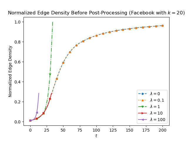
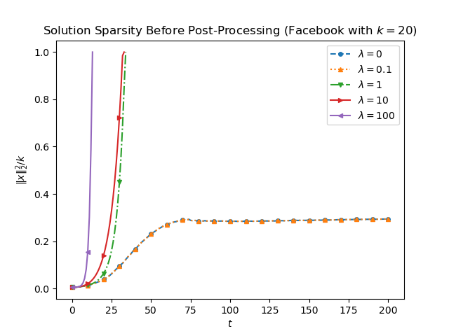
Figure 1: The comparison of different diagonal loading parameters for the Facebook dataset.

4.5 Step size selection for Frank-Wolfe

Figure 2 demonstrates that although Option I in Algorithm 1 does not guarantee a convergence rate of $O(1/\sqrt{t})$ like Option II, Option I offers much faster convergence rate than Option II. Therefore, we adopt Option I as the step size for the Frank-Wolfe algorithm.

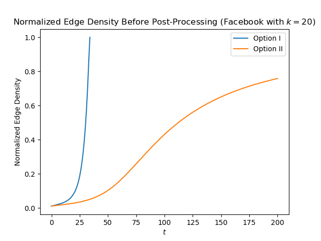
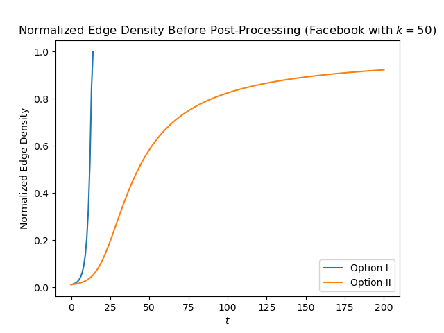
Figure 2: The comparison of the Frank-Wolfe algorithm with different step sizes for the Facebook dataset.

4.6 Comparison with Baselines

Figures 3 and 4 show the normalized edge density and the execution time of the two proposed algorithms and baselines on various datasets and different subgraph sizes. Through Figure 3 and 4, we have the following observations:

• The proposed Frank-Wolfe algorithm generally yields better subgraph density in the vast majority of cases, while also exhibiting lower computational cost compared to other algorithms that achieve similar subgraph density.

• Using the AdamW optimizer to solve the proposed parameterized optimization problem yields better subgraph density in certain cases, but overall it does not outperform the proposed Frank-Wolfe algorithm. This may be related to the landscape of the parameterized optimization problem, which may not be as favorable as that of the original optimization problem. The high computational cost of AdamW is partially attributable to the fact that matrix computations in PyTorch are more costly than those in NumPy.

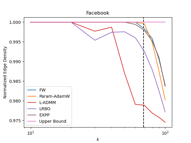
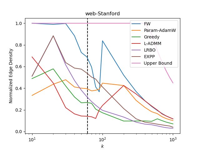
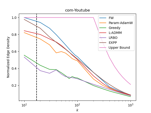
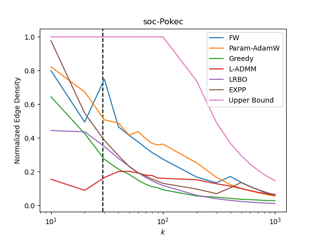
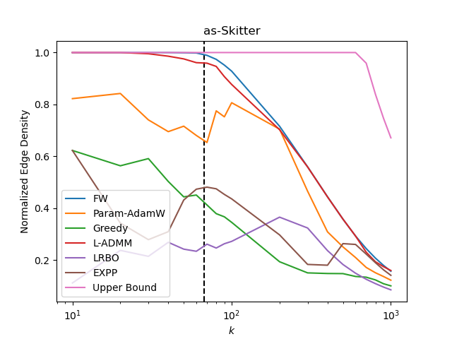
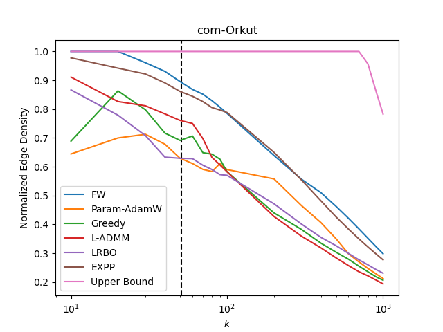
Figure 3: Normalized edge density versus subgraph size (the dashed line indicates the size of the largest clique. The greedy algorithm is omitted in Facebook to bring out the differences among the other algorithms).

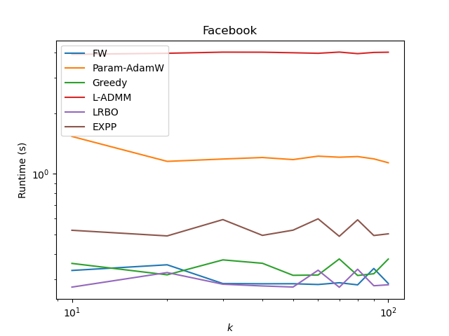
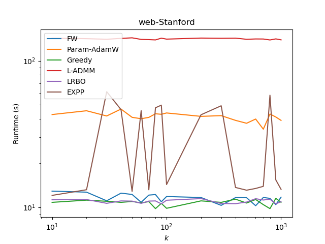
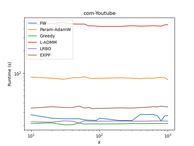
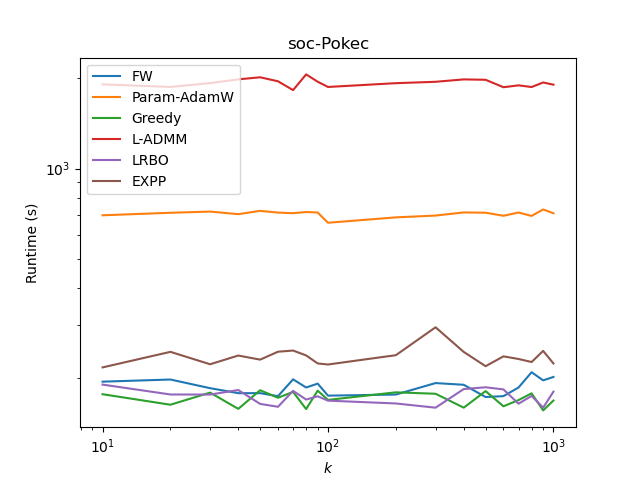
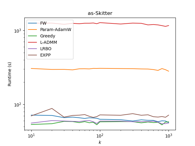
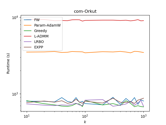
Figure 4: Execution time versus subgraph size.

5 Conclusion

In this paper, we considered the D$k$S problem. We first reformulated the D$k$S problem through diagonal loading, and then relax the combinatorial sum-to-$k$ constraint $\boldsymbol{x}\in\mathcal{B}_{k}^{n}$ to its convex hull. We proved that $\lambda=1$ is the minimum value of the diagonal loading parameter to ensure the tightness of this relaxation by leveraging an extension of the Motzkin-Straus theorem and an extension of Lemma 5.1 in [29] that we also proved herein. We also justified the importance of the diagonal loading parameter choice through landscape analysis. We proposed two projection-free approaches to solve the relaxed optimization problem. The first approach is based on the Frank-Wolfe algorithm, while the second approach involves first reformulating the relaxed optimization problem to a new unconstrained optimization problem and then solving the new optimization problem using AdamW. We experimentally verified the effectiveness of diagonal loading with parameter $\lambda=1$ and the relaxation. Experimental results show that the Frank-Wolfe algorithm is relatively lightweight and a top performer in most cases considered. It also scales well to large networks with millions of vertices.

6 Acknowledgments

This research has been supported in part by NSF IIS-1908070. The authors would like to thank Ya Liu, Junbin Liu, and Professor Wing-Kin Ma for sharing their code for [36] as a baseline for comparison.

Appendix A Proof of Theorem 2

Proof.

Let $\mathcal{M}(\boldsymbol{x})=\{i\in[n]\mid 0<x_{i}<1\}$. The set $\mathcal{M}(\boldsymbol{x})$ denotes the indices of all entries in $\boldsymbol{x}$ that are not integers. Since the cardinality of $\mathcal{M}(\boldsymbol{x})$ is either 0 or strictly greater than 1, for any non-integral feasible $\boldsymbol{x}$, we can always find two distinct vertices $i,j\in\mathcal{M}(\boldsymbol{x})$ such that $\lambda x_{i}+s_{i}\geq\lambda x_{j}+s_{j}$, where $s_{i}=\sum_{(i,l)\in\mathcal{E}}x_{l}$, $\forall i\in[n]$.

Let $\delta=\min\{x_{j},1-x_{i}\}$ and $\boldsymbol{d}=\boldsymbol{e}_{i}-\boldsymbol{e}_{j}$, where $\boldsymbol{e}_{i}$ is the $i$-th vector of the canonical basis for $\mathbb{R}^{n}$, and $\hat{\boldsymbol{x}}=\boldsymbol{x}+\delta\boldsymbol{d}$. Clearly, $\hat{\boldsymbol{x}}$ is still feasible. Next, we discuss the relationship between $g(\boldsymbol{x})$ and $g(\hat{\boldsymbol{x}})$ in two cases.

• If $(i,j)\not\in\mathcal{E}$, then we have

  $$g(\hat{\boldsymbol{x}})-g(\boldsymbol{x})$$ (27)

  $$= 2(x_{i}+\delta)s_{i}+\lambda(x_{i}+\delta)^{2}+2(x_{j}-\delta)s_{j}+\lambda(x_{j}-\delta)^{2}-2x_{i}s_{i}-\lambda x_{i}^{2}$$

  $$-2x_{j}s_{j}-\lambda x_{j}^{2}$$

  $$= 2\delta(\lambda x_{i}+s_{i}-\lambda x_{j}-s_{j})+2\lambda\delta^{2}$$

  $$\geq 0.$$

• If $(i,j)\in\mathcal{E}$, then we have

  $$g(\hat{\boldsymbol{x}})-g(\boldsymbol{x})$$ (28)

  $$= 2(x_{i}+\delta)(s_{i}-x_{j})+\lambda(x_{i}+\delta)^{2}+2(x_{j}-\delta)(s_{j}-x_{i})+\lambda(x_{j}-\delta)^{2}$$

  $$+2(x_{i}+\delta)(x_{j}-\delta)-2x_{i}s_{i}-\lambda x_{i}^{2}-2x_{j}s_{j}-\lambda x_{j}^{2}-2x_{i}x_{j}$$

  $$= 2\delta(\lambda x_{i}+s_{i}-\lambda x_{j}-s_{j})+2(\lambda-1)\delta^{2}$$

  $$\geq 0.$$

Note that the appearance of the constant 2 in (27) and (28) is because the quadratic form $\boldsymbol{x}^{\mathsf{T}}\boldsymbol{Ax}$ calculates each edge twice.

Therefore, the objective function value $g(\hat{\boldsymbol{x}})$ is greater than or equal to the objective function value $g(\boldsymbol{x})$ and the cardinality of $\mathcal{M}(\hat{\boldsymbol{x}})$ is strictly smaller than the cardinality of $\mathcal{M}(\boldsymbol{x})$. Repeat this update until the cardinality of $\mathcal{M}(\boldsymbol{x})$ reduces to 0, and we obtain an integral feasible $\boldsymbol{x}^{\prime}$ of (3) such that $g(\boldsymbol{x}^{\prime})\geq g(\boldsymbol{x})$. ∎

Appendix B Proof of Theorem 4

Proof.

We first show that $g^{*}\geq 1+\frac{\lambda-1}{\omega}$. Let

$$x_{i}=\begin{cases}\frac{1}{\omega},\text{ if vertex }i\text{ is in the largest clique},\\ 0,\text{ otherwise.}\end{cases}$$ (29)

then

$$g(\boldsymbol{x})=1-\frac{1}{\omega}+\frac{\lambda\omega}{\omega^{2}}=1+\frac{\lambda-1}{\omega}.$$ (30)

Now we show that $g^{*}\leq 1+\frac{\lambda-1}{\omega}$ by induction.

Base Case ($\boldsymbol{n}$ = 2):

• If the graph is not connected ($\omega=1$), then $g^{*}=\lambda$ when $x_{1}=1$ or $x_{2}=1$.

• If the graph is connected ($\omega=2$), then

  $$g^{*}=\max_{\boldsymbol{x}\in\Delta_{2}}2x_{1}x_{2}+\lambda(x_{1}^{2}+x_{2}^{2})=\frac{1+\lambda}{2}.$$ (31)

  when $x_{1}=x_{2}=\frac{1}{2}$.

Inductive Step: Assume that $g^{*}\leq 1+\frac{\lambda-1}{\omega}$ holds for any unweighted, undirected, and simple graph with at most $n-1$ ($n>2$) vertices. Let $\boldsymbol{x}^{*}\in\arg\max_{\boldsymbol{x}\in\Delta_{n}}g(x)$.

• If there exists a vertex $i$ such that $x_{i}^{*}=0$, we can obtain $\mathcal{G}^{\prime}$ by removing vertex $i$ from $\mathcal{G}$. Let $\boldsymbol{A}^{\prime}$ be the adjacency matrix of $\mathcal{G}^{\prime}$, $g^{\prime}(\boldsymbol{x})=\boldsymbol{x}^{\mathsf{T}}(\boldsymbol{A}^{\prime}+\lambda\boldsymbol{I})\boldsymbol{x}$, and $\boldsymbol{x}^{\prime}\in\arg\max_{\boldsymbol{x}\in\Delta_{n-1}}g^{\prime}(\boldsymbol{x})$. By induction, we know that

  $$g^{*}=g(\boldsymbol{x}^{*})\leq g^{\prime}(\boldsymbol{x}^{\prime})\leq 1+\frac{\lambda-1}{\omega^{\prime}}\leq 1+\frac{\lambda-1}{\omega}.$$ (32)

  where $\omega^{\prime}$ is the size of the largest clique of $\mathcal{G}^{\prime}$ and $\omega\geq\omega^{\prime}$ because the largest clique of $\mathcal{G}^{\prime}$ is also a clique of $\mathcal{G}$.

• If $x_{i}^{*}>0$, $\forall i\in[n]$, and $\mathcal{G}$ is not a complete graph, we assume that edge (1, 2) is missing without loss of generality. Let $\boldsymbol{x}^{\prime\prime}=[x_{1}^{*}+t,x_{2}^{*}-t,x_{3}^{*},\dots,x_{n}^{*}]^{\mathsf{T}}$ and $f(\boldsymbol{x})=\boldsymbol{x}^{\mathsf{T}}\boldsymbol{Ax}$. By leveraging the necessary optimality conditions for constrained optimization problems (see [50, p. 7] for details), it follows that

  $$f(\boldsymbol{x}^{*})=f(\boldsymbol{x}^{\prime\prime}),\forall t\in\mathbb{R}.$$ (33)

  Since $\|\boldsymbol{x}^{*}\|_{2}^{2}<\|\boldsymbol{x}^{\prime\prime}\|_{2}^{2}$ when $x_{1}^{*}+t=0$ or $x_{2}^{*}-t=0$ and $g(\boldsymbol{x})=f(\boldsymbol{x})+\lambda\|\boldsymbol{x}\|_{2}^{2}$, we know that

  $$g(\boldsymbol{x}^{*})\leq g(\boldsymbol{x}^{\prime\prime}).$$ (34)

  Hence, based on the case that there exists a vertex $i$ such that $x_{i}^{*}=0$, we know that

  $$g^{*}=g(\boldsymbol{x}^{*})\leq g(\boldsymbol{x}^{\prime\prime})\leq 1+\frac{\lambda-1}{\omega}.$$ (35)

• If $x_{i}^{*}>0$, $\forall i\in[n]$, and $\mathcal{G}$ is a complete graph ($\omega=n$), then

  $$g(\boldsymbol{x})= \left(\sum_{i\in[n]}x_{i}\right)^{2}-\sum_{i\in[n]}x_{i}^{2}+\lambda\sum_{i\in[n]}x_{i}^{2}$$ (36)

  $$= (\lambda-1)\sum_{i\in[n]}x_{i}^{2}+1.$$

  Since $g(\boldsymbol{x})$ is maximized when $x_{i}^{*}=\frac{1}{n},\forall i\in[n]$, we know that

  $$g^{*}=g(\boldsymbol{x}^{*})=1+\frac{\lambda-1}{n}.$$ (37)

Conclusion: Therefore, $g^{*}\leq 1+\frac{\lambda-1}{\omega}$ by induction which further implies that $g^{*}=1+\frac{\lambda-1}{\omega}$. ∎

Appendix C Proof of Lemma 1

Proof.

Suppose that $\boldsymbol{x}$ is a non-integral feasible point of (5). Let $\mathcal{M}(\boldsymbol{x})=\{i\in[n]\mid 0<x_{i}<1\}$. The set $\mathcal{M}(\boldsymbol{x})$ denotes the indices of all entries in $\boldsymbol{x}$ that are not integers. Since the cardinality of $\mathcal{M}(\boldsymbol{x})$ is either 0 or strictly greater than 1, for any non-integral feasible $\boldsymbol{x}$, we can always find two distinct vertices $i,j\in\mathcal{M}(\boldsymbol{x})$ such that $\lambda x_{i}+s_{i}\geq\lambda x_{j}+s_{j}$, where $s_{i}=\sum_{(i,l)\in\mathcal{E}}x_{l}$, $\forall i\in[n]$.

Let $\hat{\delta}=\min\{x_{j},1-x_{i}\}$ and $\boldsymbol{d}=\boldsymbol{e}_{i}-\boldsymbol{e}_{j}$, where $\boldsymbol{e}_{i}$ is the $i$-th vector of the canonical basis for $\mathbb{R}^{n}$. We show that $g(\boldsymbol{x}+\delta\boldsymbol{d})>g(\boldsymbol{x})$, for every $\delta\in(0,\hat{\delta}]$ in two cases.

• If $(i,j)\not\in\mathcal{E}$, then we have

  $$g(\boldsymbol{x}+\delta\boldsymbol{d})-g(\boldsymbol{x})$$ (38)

  $$= 2(x_{i}+\delta)s_{i}+\lambda(x_{i}+\delta)^{2}+2(x_{j}-\delta)s_{j}+\lambda(x_{j}-\delta)^{2}-2x_{i}s_{i}-\lambda x_{i}^{2}$$

  $$-2x_{j}s_{j}-\lambda x_{j}^{2}$$

  $$= 2\delta(\lambda x_{i}+s_{i}-\lambda x_{j}-s_{j})+2\lambda\delta^{2}$$

  $$> 0.$$

• If $(i,j)\in\mathcal{E}$, then we have

  $$g(\boldsymbol{x}+\delta\boldsymbol{d})-g(\boldsymbol{x})$$ (39)

  $$= 2(x_{i}+\delta)(s_{i}-x_{j})+\lambda(x_{i}+\delta)^{2}+2(x_{j}-\delta)(s_{j}-x_{i})+\lambda(x_{j}-\delta)^{2}$$

  $$+2(x_{i}+\delta)(x_{j}-\delta)-2x_{i}s_{i}-\lambda x_{i}^{2}-2x_{j}s_{j}-\lambda x_{j}^{2}-2x_{i}x_{j}$$

  $$= 2\delta(\lambda x_{i}+s_{i}-\lambda x_{j}-s_{j})+2(\lambda-1)\delta^{2}$$

  $$> 0.$$

Similar to the proof in Appendix A, the appearance of the constant 2 in (38) and (39) is because the quadratic form $\boldsymbol{x}^{\mathsf{T}}\boldsymbol{Ax}$ calculates each edge twice. Therefore, $\boldsymbol{d}=\boldsymbol{e}_{i}-\boldsymbol{e}_{j}$ is an ascent direction at $\boldsymbol{x}$, which implies that $\boldsymbol{x}$ is not a local maximizer of (5). ∎

Appendix D Proof of Theorem 5

Proof.

Since $\boldsymbol{x}$ is a local maximizer of (5) with diagonal loading parameter $\lambda_{1}$, there exists $\epsilon>0$, such that $\boldsymbol{x}^{\mathsf{T}}(\boldsymbol{A}+\lambda_{1}\boldsymbol{I})\boldsymbol{x}\geq\boldsymbol{y}^{\mathsf{T}}(\boldsymbol{A}+\lambda_{1}\boldsymbol{I})\boldsymbol{y}$ for every $\boldsymbol{y}\in\mathcal{C}_{\epsilon}$, where $\mathcal{C}_{\epsilon}=\{\boldsymbol{y}\in\mathcal{C}_{k}^{n}\mid\|\boldsymbol{x}-\boldsymbol{y}\|_{2}\leq\epsilon\}$. Now, we only need to show that $\boldsymbol{x}^{\mathsf{T}}(\boldsymbol{A}+\lambda_{2}\boldsymbol{I})\boldsymbol{x}\geq\boldsymbol{y}^{\mathsf{T}}(\boldsymbol{A}+\lambda_{2}\boldsymbol{I})\boldsymbol{y}$ for every $\boldsymbol{y}\in\mathcal{C}_{\epsilon}$. From Lemma 1, we know that $\boldsymbol{x}$ is integral, which implies that

$$\boldsymbol{x}^{\mathsf{T}}(\boldsymbol{A}+\lambda_{2}\boldsymbol{I})\boldsymbol{x}-\boldsymbol{y}^{\mathsf{T}}(\boldsymbol{A}+\lambda_{2}\boldsymbol{I})\boldsymbol{y}$$ (40)

$$= \boldsymbol{x}^{\mathsf{T}}(\boldsymbol{A}+\lambda_{1}\boldsymbol{I})\boldsymbol{x}+(\lambda_{2}-\lambda_{1})\|\boldsymbol{x}\|_{2}^{2}-\boldsymbol{y}^{\mathsf{T}}(\boldsymbol{A}+\lambda_{1}\boldsymbol{I})\boldsymbol{y}-(\lambda_{2}-\lambda_{1})\|\boldsymbol{y}\|_{2}^{2}$$

$$\geq (\lambda_{2}-\lambda_{1})(\|\boldsymbol{x}\|_{2}^{2}-\|\boldsymbol{y}\|_{2}^{2})$$

$$\geq 0,$$

where the last inequality holds because $\|\boldsymbol{z}\|_{2}^{2}$ is maximized over $\mathcal{C}_{k}^{n}$ when $\boldsymbol{z}$ is integral.

Therefore, $\boldsymbol{x}$ is also a local maximizer of (5) with diagonal loading parameter $\lambda_{2}$. ∎

References

- [1] T. Lanciano, A. Miyauchi, A. Fazzone, and F. Bonchi, “A survey on the densest subgraph problem and its variants,” ACM Computing Surveys, vol. 56, no. 8, pp. 1–40, 2024.
- [2] W. Luo, C. Ma, Y. Fang, and L. V. Lakshman, “A survey of densest subgraph discovery on large graphs,” arXiv preprint arXiv:2306.07927, 2023.
- [3] E. Fratkin, B. T. Naughton, D. L. Brutlag, and S. Batzoglou, “Motifcut: Regulatory motifs finding with maximum density subgraphs,” Bioinformatics, vol. 22, no. 14, pp. e150–e157, 2006.
- [4] A. Angel, N. Koudas, N. Sarkas, D. Srivastava, M. Svendsen, and S. Tirthapura, “Dense subgraph maintenance under streaming edge weight updates for real-time story identification,” The VLDB Journal, vol. 23, pp. 175–199, 2014.
- [5] B. Saha, A. Hoch, S. Khuller, L. Raschid, and X.-N. Zhang, “Dense subgraphs with restrictions and applications to gene annotation graphs,” in 14th International Conference on Research in Computational Molecular Biology (RECOMB 2010), pp. 456–472, Springer, 2010.
- [6] B. Hooi, H. A. Song, A. Beutel, N. Shah, K. Shin, and C. Faloutsos, “Fraudar: Bounding graph fraud in the face of camouflage,” in Proceedings of the 22nd ACM SIGKDD International Conference on Knowledge Discovery and Data Mining, pp. 895–904, ACM, 2016.
- [7] X. Li, S. Liu, Z. Li, X. Han, C. Shi, B. Hooi, H. Huang, and X. Cheng, “Flowscope: Spotting money laundering based on graphs,” in Proceedings of the AAAI Conference on Artificial Intelligence, vol. 34, pp. 4731–4738, 2020.
- [8] Y. Ji, Z. Zhang, X. Tang, J. Shen, X. Zhang, and G. Yang, “Detecting cash-out users via dense subgraphs,” in Proceedings of the 28th ACM SIGKDD Conference on Knowledge Discovery and Data Mining, pp. 687–697, ACM, 2022.
- [9] T. Chen and C. Tsourakakis, “Antibenford subgraphs: Unsupervised anomaly detection in financial networks,” in Proceedings of the 28th ACM SIGKDD Conference on Knowledge Discovery and Data Mining, pp. 2762–2770, ACM, 2022.
- [10] A. V. Goldberg, “Finding a maximum density subgraph,” tech. rep., 1984.
- [11] M. Charikar, “Greedy approximation algorithms for finding dense components in a graph,” in International Workshop on Approximation Algorithms for Combinatorial Optimization, pp. 84–95, Springer, 2000.
- [12] D. Boob, Y. Gao, R. Peng, S. Sawlani, C. Tsourakakis, D. Wang, and J. Wang, “Flowless: Extracting densest subgraphs without flow computations,” in Proceedings of The Web Conference 2020, pp. 573–583, ACM, 2020.
- [13] C. Chekuri, K. Quanrud, and M. R. Torres, “Densest subgraph: Supermodularity, iterative peeling, and flow,” in Proceedings of the 2022 Annual ACM-SIAM Symposium on Discrete Algorithms (SODA), pp. 1531–1555, SIAM, 2022.
- [14] S. B. Seidman, “Network structure and minimum degree,” Social Networks, vol. 5, no. 3, pp. 269–287, 1983.
- [15] N. Veldt, A. R. Benson, and J. Kleinberg, “The generalized mean densest subgraph problem,” in Proceedings of the 27th ACM SIGKDD Conference on Knowledge Discovery & Data Mining, pp. 1604–1614, ACM, 2021.
- [16] C. Tsourakakis, F. Bonchi, A. Gionis, F. Gullo, and M. Tsiarli, “Denser than the densest subgraph: Extracting optimal quasi-cliques with quality guarantees,” in Proceedings of the 19th ACM SIGKDD International Conference on Knowledge Discovery and Data Mining, pp. 104–112, ACM, 2013.
- [17] K. Shin, T. Eliassi-Rad, and C. Faloutsos, “Corescope: Graph mining using -core analysis — patterns, anomalies and algorithms,” in 2016 IEEE 16th International Conference on Data Mining (ICDM), pp. 469–478, IEEE, 2016.
- [18] U. Feige, D. Peleg, and G. Kortsarz, “The dense -subgraph problem,” Algorithmica, vol. 29, pp. 410–421, 2001.
- [19] S. Khot, “Ruling Out PTAS for Graph Min-Bisection, Dense -Subgraph, and Bipartite Clique,” SIAM Journal on Computing, vol. 36, no. 4, pp. 1025–1071, 2006.
- [20] P. Manurangsi, “Almost-polynomial ratio eth-hardness of approximating densest -subgraph,” in Proceedings of the 49th Annual ACM SIGACT Symposium on Theory of Computing, pp. 954–961, ACM, 2017.
- [21] R. Andersen and K. Chellapilla, “Finding dense subgraphs with size bounds,” in International Workshop on Algorithms and Models for the Web-Graph, pp. 25–37, Springer, 2009.
- [22] S. Khuller and B. Saha, “On finding dense subgraphs,” in International Colloquium on Automata, Languages, and Programming, pp. 597–608, Springer, 2009.
- [23] Y. Kawase and A. Miyauchi, “The densest subgraph problem with a convex/concave size function,” Algorithmica, vol. 80, pp. 3461–3480, 2018.
- [24] A. Bhaskara, M. Charikar, E. Chlamtac, U. Feige, and A. Vijayaraghavan, “Detecting high log-densities: an approximation for densest -subgraph,” in Proceedings of the Forty-Second ACM Symposium on Theory of Computing, pp. 201–210, ACM, 2010.
- [25] A. Bhaskara, M. Charikar, V. Guruswami, A. Vijayaraghavan, and Y. Zhou, “Polynomial integrality gaps for strong sdp relaxations of densest -subgraph,” in Proceedings of the Twenty-Third Annual ACM-SIAM Symposium on Discrete Algorithms, pp. 388–405, SIAM, 2012.
- [26] B. P. Ames, “Guaranteed recovery of planted cliques and dense subgraphs by convex relaxation,” Journal of Optimization Theory and Applications, vol. 167, pp. 653–675, 2015.
- [27] J. Eckstein and D. P. Bertsekas, “On the Douglas—Rachford splitting method and the proximal point algorithm for maximal monotone operators,” Mathematical Programming, vol. 55, pp. 293–318, 1992.
- [28] P. Bombina and B. Ames, “Convex optimization for the densest subgraph and densest submatrix problems,” in SN Operations Research Forum, vol. 1, pp. 1–24, Springer, 2020.
- [29] S. Barman, “Approximating Nash equilibria and dense subgraphs via an approximate version of Carathéodory’s theorem,” SIAM Journal on Computing, vol. 47, no. 3, pp. 960–981, 2018.
- [30] X.-T. Yuan and T. Zhang, “Truncated power method for sparse eigenvalue problems,” Journal of Machine Learning Research, vol. 14, no. 28, pp. 899–925, 2013.
- [31] D. Papailiopoulos, I. Mitliagkas, A. Dimakis, and C. Caramanis, “Finding dense subgraphs via low-rank bilinear optimization,” in Proceedings of the 31st International Conference on Machine Learning, pp. 1890–1898, PMLR, 2014.
- [32] W. W. Hager, D. T. Phan, and J. Zhu, “Projection algorithms for nonconvex minimization with application to sparse principal component analysis,” Journal of Global Optimization, vol. 65, pp. 657–676, 2016.
- [33] R. Sotirov, “On solving the densest -subgraph problem on large graphs,” Optimization Methods and Software, vol. 35, no. 6, pp. 1160–1178, 2020.
- [34] A. Konar and N. D. Sidiropoulos, “Exploring the subgraph density-size trade-off via the Lovaśz extension,” in Proceedings of the 14th ACM International Conference on Web Search and Data Mining, p. 743–751, ACM, 2021.
- [35] L. Condat, “A primal-dual splitting method for convex optimization involving Lipschitzian, proximable and linear composite terms,” Journal of Optimization Theory and Applications, vol. 158, no. 2, pp. 460–479, 2013.
- [36] Y. Liu, J. Liu, and W.-K. Ma, “Cardinality-constrained binary quadratic optimization via extreme point pursuit, with application to the densest k-subgraph problem,” in 2024 IEEE International Conference on Acoustics, Speech and Signal Processing (ICASSP), pp. 9631–9635, 2024.
- [37] T. S. Motzkin and E. G. Straus, “Maxima for graphs and a new proof of a theorem of Turán,” Canadian Journal of Mathematics, vol. 17, p. 533–540, 1965.
- [38] R. T. Rockafellar, Convex Analysis. Princeton, NJ: Princeton University Press, 1970.
- [39] M. Frank and P. Wolfe, “An algorithm for quadratic programming,” Naval Research Logistics Quarterly, vol. 3, no. 1-2, pp. 95–110, 1956.
- [40] M. Jaggi, “Revisiting Frank-Wolfe: Projection-free sparse convex optimization,” in Proceedings of the 30th International Conference on Machine Learning, pp. 427–435, PMLR, 2013.
- [41] M. Danisch, T.-H. H. Chan, and M. Sozio, “Large scale density-friendly graph decomposition via convex programming,” in Proceedings of the 26th International Conference on World Wide Web, pp. 233–242, 2017.
- [42] D. Bertsekas, Nonlinear Programming. Belmont, MA: Athena Scientific, 3rd ed., 2016.
- [43] S. Lacoste-Julien, “Convergence rate of Frank-Wolfe for non-convex objectives,” arXiv preprint arXiv:1607.00345, 2016.
- [44] D. P. Kingma and J. Ba, “Adam: A method for stochastic optimization,” in International Conference on Learning Representations, 2015.
- [45] I. Loshchilov and F. Hutter, “Decoupled weight decay regularization,” in International Conference on Learning Representations, 2019.
- [46] J. Leskovec and A. Krevl, “SNAP Datasets: Stanford large network dataset collection.” http://snap.stanford.edu/data, June 2014.
- [47] A. Jursa, “Fast algorithm for finding maximum clique in scale-free networks.,” in Proceedings of the 16th ITAT Conference Information Technologies - Applications and Theory, pp. 212–217, 2016.
- [48] S. Jain and C. Seshadhri, “The power of pivoting for exact clique counting,” in Proceedings of the 13th International Conference on Web Search and Data Mining, p. 268–276, ACM, 2020.
- [49] A. Paszke, S. Gross, F. Massa, A. Lerer, J. Bradbury, G. Chanan, T. Killeen, Z. Lin, N. Gimelshein, L. Antiga, A. Desmaison, A. Kopf, E. Yang, Z. DeVito, M. Raison, A. Tejani, S. Chilamkurthy, B. Steiner, L. Fang, J. Bai, and S. Chintala, “Pytorch: An imperative style, high-performance deep learning library,” in Advances in Neural Information Processing Systems, vol. 32, Curran Associates, Inc., 2019.
- [50] A. A. Ahmadi, “ORF 523 Convex and Conic Optimization, Lecture 14: Complexity of Local Optimization, the Motzkin-Straus Theorem, Matrix Copositivity.” Lecture Notes, Princeton University, 2018.