Nonlinear resonant interactions of radiation belt electrons with intense whistler-mode waves.

Abstract

The dynamics of the Earth’s outer radiation belt, filled by energetic electron fluxes, is largely controlled by electron resonant interactions with electromagnetic whistler-mode waves. The most coherent and intense waves resonantly interact with electrons nonlinearly, and the observable effects of such nonlinear interactions cannot be described within the frame of classical quasi-linear models. This paper provides an overview of the current stage of the theory of nonlinear resonant interactions and discusses different possible approaches for incorporating these nonlinear interactions into global radiation belt simulations. We focused on observational properties of whistler-mode waves and theoretical aspects of electron nonlinear resonant interactions between such waves and energetic electrons.

1 Introduction

The outer radiation belt is a near-Earth magnetospheric region filled with energetic electrons reaching relativistic and even ultra-relativistic energies Horne et al. [2005]; Horne [2007]; Baker et al. [2014, 2016]; Allison & Shprits [2020]. The potentially significant damaging effects of relativistic electron fluxes for the many satellites on orbit continuously drives investigation, modelling, and forecasting of the radiation belt dynamics Horne, Glauert, Meredith, Boscher, Maget, Heynderickx & Pitchford [2013]; Baker et al. [2018]. Although the magnetic field in the outer radiation belt is dominated by the quite stable dipole field of the Earth, energetic electron fluxes in this region may vary by several orders of magnitude. Wave-particle resonant interaction is the main driver of such flux variations: the radial drift of energetic electrons is provided by drift resonance with ultra-low-frequency (ULF) waves, whereas bounce and cyclotron resonances with extremely and very-low-frequency (ELF/VLF) waves are responsible for electron pitch-angle scattering and energization Lyons & Williams [1984]; Schulz & Lanzerotti [1974]; Tverskoy [1969]; Trakhtengerts & Rycroft [2008]. Without wave-particle resonant interactions, since electrons are magnetized by the strong dipolar geomagnetic field, three adiabatic invariants are conserved during electron motion, corresponding to three types of electron periodical motions: the magnetic moment, $\mu$, corresponds to the gyrorotation, the bounce invariant, $J_{\parallel}$, corresponds to bounce oscillations along field lines, and the third invariant, $\Phi$, corresponds to the azimuthal drift motion around the Earth (see schematic 1 and Schulz & Lanzerotti [1974]; Tverskoy [1969]). The conservation of these invariants can fix the electron energy $\gamma=E/m_{e}c^{2}$ and equatorial pitch-angle $\alpha_{eq}$, and the $L$-shell, the normalized distance between the Earth center and the farthest (equatorial) point of the magnetic field line along which electrons are bouncing at every point along the electron drift orbit. Therefore, any change of electron phase space density should be attributed to destruction of one or more of these invariants.

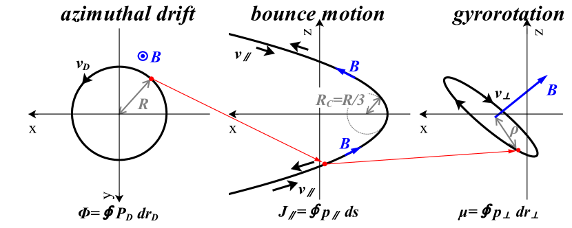
Figure 1: Schematic view of electron motion in dipole magnetic field. Three types of periodical motions are shown (from left to right): azimuthal drift around the Earth with the invariant $\Phi=\oint{P_{D}dr_{D}}$ where $P_{D}=eA_{\Phi}/c+mv_{D}\approx eA_{\Phi}/c$ is the azimuthal momentum and $dr_{D}=Rd\Phi$ is the element of azimuthal trajectory; bounce motion along magnetic field lines between mirror points with the invariant $J_{\parallel}=\oint{p_{\parallel}ds}$ where $s$ is the field aligned coordinate; gyrorotation around the magnetic field with the invariant $\mu=\oint{p_{\perp}dr_{\perp}}$ where $(p_{\parallel},p_{\perp})$ are parallel and perpendicular momentum components. The direction of the magnetic field is shown in blue. In dipole field $R=R_{E}L$ ($R_{E}$ is the Earth radius and $L$ is the $L$-shell parameter), the magnetic field inhomogeneity scale along magnetic field lines is the curvature radius $R_{C}=R/3$, the electron gyroradius $\rho\ll R$.

Adiabatic invariants are conserved exponentially well Kulsrud [1957]; Lenard [1959]; Dykhne [1960]; Slutskin [1964]; Cohen et al. [1978]; Neishtadt [2000], and their destruction requires the action of a force varying in space or time faster than the spatial/temporal scale of the periodic motion corresponding to the specific invariant [e.g., Roberts, 1969]. For example, destruction of $\Phi$ requires some external force with a temporal scale comparable to the electron azimuthal drift period, whereas violation of $\mu$ requires an external force with a temporal scale comparable to the electron gyroperiod. Such external forces can be Lorentz force of wave electromagnetic fields varying with the corresponding temporal scales. Figure 2 shows an example of such invariant violation for the electron resonant interaction with circularly polarized electromagnetic waves. Each resonant interaction lasts for a short interval during which the adiabatic invariant experiences a random jump, whereas the longer time intervals between resonant interactions are characterized by conservation of the adiabatic invariant, when the particle is bouncing or drifting far from the wave region.

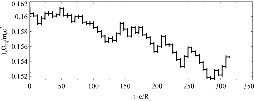
Figure 2: Example of electron resonant interactions with a field-aligned whistler-mode wave: effect of electron scattering and magnetic moment violation is shown. Plots show the electron magnetic moment $I_{x}=m_{e}c^{2}(\gamma^{2}-1)\sin^{2}\alpha/\Omega_{0}$ along the particle trajectory during half of an electron bounce period in a dipole magnetic field. System parameters are: whistler-mode wave frequency equal to $0.35$ of equatorial electron gyrofrequency, wave magnetic field amplitude is $10$ pT, the background magnetic field is dipolar Bell [1984] with $L-$shell equal to $6$, equatorial plasma density is given by an empirical model [Sheeley et al., 2001] and it is constant along magnetic field lines. The magnetic moment is $\mu=eI_{x}/m_{e}c$, and time is normalized to $c/R$ with $R=LR_{E}$, with $R_{E}$ the Earth radius. The total time of this simulation is $\sim 41$s.

Therefore, the primary theoretical problem for evaluation of the radiation belt dynamics is to develop an approach describing the evolution of the electron phase space density $f$ due to multiple resonances with realistic electromagnetic waves. Let us start our introduction to this problem with a brief description of a well developed, and most frequently used, theoretical concept of such evolution – quasi-linear theory MacDonald & Walt [1961]; Vedenov et al. [1962]; Drummond & Pines [1962]; Trakhtengerts [1963]; Wentworth [1963]; Kennel & Engelmann [1966]; Kennel & Petschek [1966]; Roberts [1969]. This theory describes the self-consistent dynamics of the charged particle distribution and of the spectrum of electromagnetic waves: waves are generated by unstable particle populations and scatter these populations, moving them in parameter space toward the equilibrium state. The two main equations of the quasi-linear theory are the Fokker-Planck (diffusion) equation

$$\frac{{\partial f_{0}}}{{\partial t}} = \frac{\partial}{{\partial p_{\bot}}}\left({D_{\bot\bot}\frac{{\partial f_{0}}}{{\partial p_{\bot}}}+D_{\bot\parallel}\frac{{\partial f_{0}}}{{\partial p_{\parallel}}}}\right)+\frac{\partial}{{\partial p_{\parallel}}}\left({D_{\parallel\parallel}\frac{{\partial f_{0}}}{{\partial p_{\parallel}}}+D_{\parallel\bot}\frac{{\partial f_{0}}}{{\partial p_{\bot}}}}\right)$$

$$+ \frac{{D_{\bot\parallel}}}{{p_{\bot}}}\frac{{\partial f_{0}}}{{\partial p_{\parallel}}}+\frac{{D_{\bot\bot}}}{{p_{\bot}}}\frac{{\partial f_{0}}}{{\partial p_{\bot}}}=\frac{\partial}{{\partial{\bf p}}}\left({\hat{D}_{{pp}}\frac{{\partial f}}{{\partial{\bf p}}}}\right)$$

and the wave spectrum equation

$$\frac{{\partial{\cal U}_{w}}}{{\partial t}}+\left({\nabla\cdot{\bf v}_{g}{\cal U}_{w}}\right)=2\gamma{\cal U}_{w}$$

where $\hat{D}_{pp}$ is the $2\times 2$ tensor consisting of diffusion coefficients in momentum space $(p_{\parallel},p_{\perp})$; and $\parallel,\perp$ are relative to the direction of the background magnetic field; ${\cal U}_{w}$ is the wave energy density, that can be expressed through the wave magnetic field energy $B_{k}^{2}$ and the Hermitian part of the dielectric tensor $\hat{\varepsilon}(\omega)$ Shklyar & Matsumoto [2009], as

$${\cal U}_{w}=\frac{1}{{16\pi\omega}}\left({{\bf E}\cdot\frac{{d\omega^{2}\hat{\varepsilon}(\omega)}}{{d\omega}}{\bf E}}\right)=\frac{1}{{16\pi}}\left({B_{k}^{2}{\bf a}\cdot\frac{{d\omega\hat{\varepsilon}(\omega)}}{{d\omega}}{\bf a}+{\bf B}^{2}}\right)=B_{k}^{2}Y,$$

where the vector ${\bf a}$ is given by the relationship between wave electric field vector and wave magnetic field magnitude ${\bf E}_{w}={\bf a}B_{k}$ and is determined by the wave dispersion relation, as well as coefficient $Y$. Note that the mostly used quasi-linear equations are written for cyclotron resonance between charged particles and electromagnetic waves and, thus, describe the system averaged over electron gyrophase, i.e., these equations reduce the initially 3D momentum space to 2D $(p_{\parallel},p_{\perp})$ space. Diffusion coefficients $\hat{D}_{pp}$ can be derived from the linear perturbation theory, the basic assumption of any quasi-linear model Vedenov et al. [1962]; Drummond & Pines [1962]; Trakhtengerts [1963]; Kennel & Engelmann [1966]. Although the initial formulation of quasi-linear theory assumes that $\hat{D}_{pp}$ should be derived for a self-consistent wave spectrum $B_{k}^{2}$, the diffusion equation is often solved only for the most energetic (or relativistic) particle population, which usually does not contribute significantly to the variation of $B_{k}^{2}$. Therefore, statistical models of the waves, measured by spacecraft, can then be used instead of numerically evaluating the self-consistent evolution of $B_{k}^{2}$ [see examples in Summers, 2005; Summers et al., 2007; Glauert & Horne, 2005; Ni et al., 2008].

The quasi-linear equations describe only diffusion $\hat{D}_{pp}\propto{\cal B}_{w}^{2}/B_{0}^{2}$ and drift $\hat{V}_{p}\nabla_{p}\hat{D}_{pp}\propto{\cal B}_{w}^{2}/B_{0}^{2}$ with ${\cal B}_{w}^{2}=\langle B_{k}^{2}\rangle$ the wave spectrum intensity. These two processes, diffusion and drift, are the results of integration of the wave Lorentz force along unperturbed particle trajectories and, thus, do not include any nonlinear effects. Nonlinearity consists in a significant role played by the wave Lorentz force in charged particle dynamics, and should manifest itself in a nonlinear dependence of diffusion on wave intensity, $\hat{D}_{pp}\propto({\cal B}_{w}/B_{0})^{\kappa}$ with $\kappa\neq 2$, strong drifts $\hat{V}_{p}\nabla_{p}\hat{D}_{pp}\propto({\cal B}_{w}/B_{0})^{\kappa}$ with $\kappa<2$, and nondiffusive/drift terms in the full kinetic equation. The latter terms are the most difficult to include in the basic numerical models of radiation belt dynamics [see discussion in Furuya et al., 2008; Artemyev, Vasiliev, Mourenas, Agapitov, Krasnoselskikh, Boscher & Rolland, 2014; Omura et al., 2015]. To explain a possible generalization of the Fokker-Planck equation suitable for including nonlinear wave-particle interactions, let us start with the general form of Smoluchowski coagulation equation Sinitsyn et al. [2011]

$$\frac{{\partial f_{0}}}{{\partial t}}=\int\limits_{-\infty}^{\infty}{\left({\hat{K}\left({\left.{\bf p}\right|{\bf p^{\prime}}}\right)f_{0}\left({{\bf p^{\prime}}}\right)-\hat{K}\left({\left.{{\bf p^{\prime}}}\right|{\bf p}}\right)f_{0}\left({\bf p}\right)}\right)d{\bf p^{\prime}}}$$ (1)

describing the evolution of $f({\bf p})$. Here, $\hat{K}({\bf p}|{\bf p’})$ is the coagulation kernel that describes the rate at which particle positions change in 2D $(p_{\parallel},p_{\perp})$ space from ${\bf p}$ to ${\bf p’}$. Thus, the first term in Eq. (1) describes the particle flux toward ${\bf p}$ and the second term describes the particle fluxes away from ${\bf p}$.

Let us assume that each resonant interaction slightly changes particle momentum, $\Delta p_{\parallel,\perp}/p\ll 1$, so that we can expand $f({\bf p’})$ as

$$f_{0}\left({{\bf p^{\prime}}}\right)=f_{0}\left({{\bf p}+\Delta{\bf p}}\right)=f_{0}\left({\bf p}\right)+\frac{{\partial f_{0}}}{{\partial{\bf p}}}\cdot\Delta{\bf p}+\frac{1}{2}\frac{{\partial^{2}f_{0}}}{{\partial{\bf p}^{2}}}\left({\Delta{\bf p}}\right)^{2}$$

Substituting this expression into Eq. (1), we obtain

$$\frac{{\partial f_{0}}}{{\partial t}} = f_{0}\left({\bf p}\right)\int\limits_{-\infty}^{\infty}{\left({\hat{K}\left({\left.{\bf p}\right|{\bf p^{\prime}}}\right)-\hat{K}\left({\left.{{\bf p^{\prime}}}\right|{\bf p}}\right)}\right)d{\bf p^{\prime}}}+\frac{{\partial f_{0}}}{{\partial{\bf p}}}\int\limits_{-\infty}^{\infty}{\hat{K}\left({\left.{\bf p}\right|{\bf p^{\prime}}}\right)\Delta{\bf p}d{\bf p^{\prime}}}$$

$$+ \frac{1}{2}\frac{{\partial^{2}f_{0}}}{{\partial{\bf p}^{2}}}\int\limits_{-\infty}^{\infty}{\hat{K}\left({\left.{\bf p}\right|{\bf p^{\prime}}}\right)\left({\Delta{\bf p}}\right)^{2}d{\bf p^{\prime}}}={\bf V}\frac{{\partial f_{0}}}{{\partial{\bf p}}}+\hat{D}_{pp}\frac{{\partial^{2}f_{0}}}{{\partial{\bf p}^{2}}}=\frac{\partial}{{\partial{\bf p}}}\left({\hat{D}_{pp}\frac{{\partial f_{0}}}{{\partial{\bf p}}}}\right)$$

where the last equality is provided by the divergence free condition ${\bf V}=\partial\hat{D}_{pp}/\partial{\bf p}$ Sinitsyn et al. [2011]; Sagdeev et al. [1988]; Lichtenberg & Lieberman [1983]. In this case, the Smoluchowski coagulation equation can be reduced to the Fokker-Planck diffusion equation:

$$\frac{{\partial f_{0}}}{{\partial t}}=\frac{\partial}{{\partial{\bf p}}}\left({\hat{D}_{pp}\frac{{\partial f_{0}}}{{\partial{\bf p}}}}\right)$$

This is the limit of the quasi-linear theory. If the resonant interaction is nonlinear, but can still be described by $\Delta p_{\parallel,\perp}/p\ll 1$, the diffusion equation is still usable, although diffusion coefficients should then be derived from test particle models including nonlinear wave field effects [see examples in Karpman & Shklyar, 1977; Inan, 1987; Shklyar, 2021; Allanson et al., 2022; Frantsuzov et al., 2023].

The most sophisticated case is when $\hat{K}$ describe large momentum changes $\Delta p_{\parallel,\perp}/p\sim 1$, and the integral operator $\sim\int\hat{K}$ cannot be reduced to the differential one. Such situation is common for electron nonlinear resonant interaction with intense whistler-mode waves [e.g., Demekhov et al., 2006; Omura et al., 2007; Bortnik et al., 2008; Agapitov et al., 2015b] and EMIC [e.g., Albert & Bortnik, 2009; Omura & Zhao, 2012; Grach & Demekhov, 2018a, 2020]. Figure 3 shows examples of electron trajectories with the large resonant changes of momentum due to the so-called phase trapping effect. A comparison of black (scattered electrons) and red (phase trapped electron) trajectories illustrates the main problem for the description of nonlinear resonant interractions with the differential operators of the Fokker-Planck equation: the momentum change for a single resonant interaction (i.e., during the interval between electron trapping into the resonance and escape from this trapping) is comparable to the initial momentum amplitude. Therefore, the inclusion of such large momentum jumps into the Fokker-Planck equation would either require a significant decrease of the typical time-step of the simulation [such that the time-step of electron distribution evolution is much smaller than the electron bounce period, and phase trapping is modelled as a combination of small consecutive energy changes, see examples in Shklyar, 1981; Foster et al., 2017], or the development of a non-differential (integral) operator describing the large energy change on the smallest system time-scale, during an electron bounce period. Therefore, the main challenge for radiation belt models is to construct $\hat{K}$ or find an approach for taking into account the effects of the integral operator $\sim\int\hat{K}$ into the diffusive Fokker-Planck equation. This review is devoted to possible solutions to this challenge.

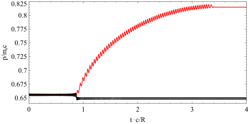
Figure 3: Examples of electron resonant interactions with a field-aligned whistler-mode wave: the effect of phase trapping is shown by red color, whereas all black trajectories show the phase bunching effect (small momentum decrease). Plot shows electron momentum $p=m_{e}c\sqrt{\gamma^{2}-1}$ for a half of an electron bounce period in a dipole magnetic field. System parameters are the same as in Fig. 2, but wave amplitude is $300$pT.

The most direct, and quite effective, approach consists in numerically evaluating the $\hat{K}$ function. This approach has been applied for test particle simulations of electron interactions with EMIC and electrostatic waves [Zheng et al., 2019; Artemyev, Vasiliev & Neishtadt, 2019], but the most elaborate variant of this approach, called the Green function approach, has been proposed for electron resonant interactions with chorus waves [Furuya et al., 2008; Omura et al., 2015]. This is the most developed and advanced approach accounting for multiple properties of resonances: wave frequency drift [Hsieh & Omura, 2017b], wave propagation in the form of a train of short wave packets [Kubota & Omura, 2018; Hiraga & Omura, 2020], wave oblique propagation [Hsieh & Omura, 2017a; Hsieh et al., 2020], multiple resonances due to wave obliqueness [Hsieh et al., 2022; Hsieh & Omura, 2023]. The main advance of this approach is that the numerical evaluation of $\hat{K}$ can be performed for an arbitrary and very realistic wave field model. The main disadvantage is that such numerical evaluation requires a discretization of the momentum space with a sufficient statistics (sufficiently large number) of resonant interactions inside each bin, whereas the lowest bin size is determined by weak diffusive scattering $\Delta p\propto{\cal B}_{w}/B_{0}$ and the range of $\Delta p$ is determined by the phase trapping property with $\Delta p\propto O({\cal B}_{w}/B_{0})\gg{\cal B}_{w}/B_{0}$. Thus, a purely numerical evaluation of $\hat{K}$ may sometimes miss some weak diffusive effects, and this approach should be mostly effective for modeling brief events with not-widely-varying system characteristics (to avoid a recalculation of $\hat{K}$ for multiple realizations of system parameters).

In this review, we examine the theoretical properties of the $\hat{K}$ function, and explore different approaches for its analytical evaluation (Sections 2, 3, and 4). We provide a detailed investigation of $\hat{K}$ for nonlinear electron interactions with monochromatic intense whistler-mode waves, and provide asymptotic solutions for the kinetic equation including such $\hat{K}$ (Sections 4). Then, we generalize $\hat{K}$ for systems with a large wave ensemble, and perform such a generalization via the mapping technique for nonlinear resonant interactions (Section 4.4). In Appendix E, we provide several examples of application of this technique for simulations of the observed dynamics of the electron flux. The next natural generalization of the theoretical approach for nonlinear wave-particle interactions consists of the inclusion of the effects of short wave-packets. We discuss the main aspects of this generalization (Section 5) and of the theoretical approaches for inclusion of short wave-packets into the mapping technique (Section 6). Next, we consider an approach allowing the incorporation of nonlinear resonant interactions into existing global numerical models of the radiation belts (Section 7). Finally we discuss several aspects of nonlinear resonant interactions that are not included in this review, but can be important for specific plasma systems (Section 8). The review also contains Appendix A, with the main equations of the Hamiltonian approach for wave-particle resonant interactions, Appendix B considering a special situation of nonlinear interactions for field-aligned particles, Appendix C describing analytical estimates for electron resonant interaction with short wave-packets, Appendix D describing the problem of the electron phase gain between two resonances, and Appendix E with several examples of observations of nonlinear resonant effects.

2 Basic properties of electron resonant interactions

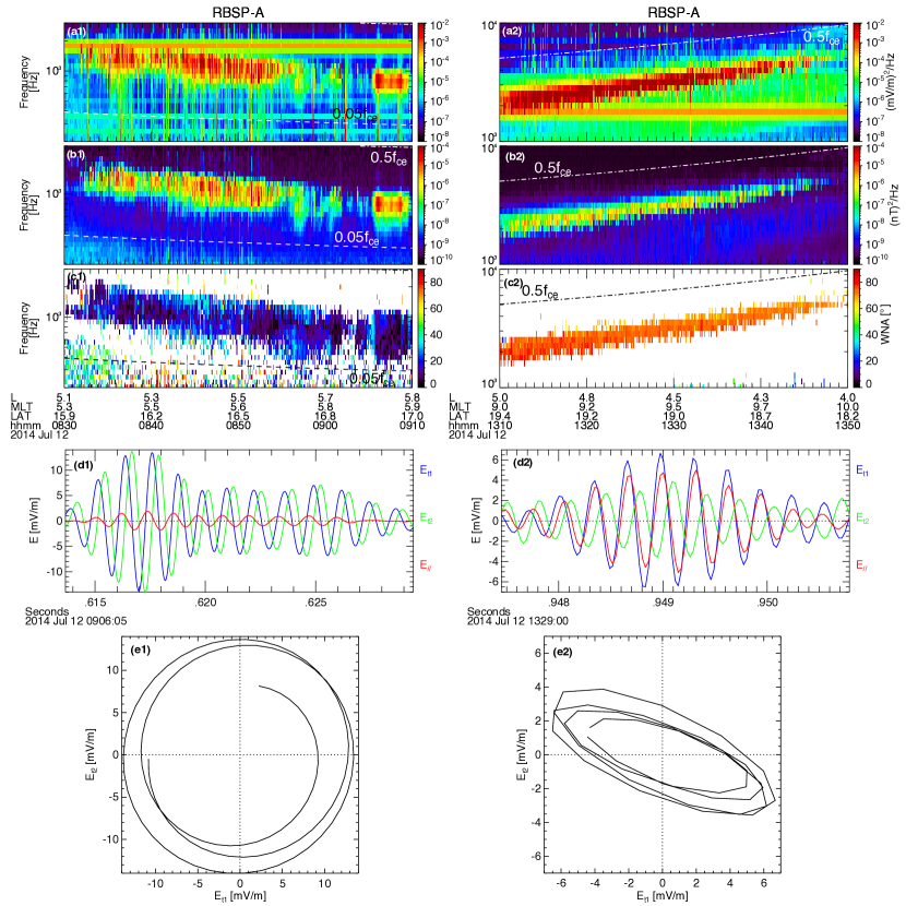
Figure 4: Two examples of whistler-mode waves (from top to bottom): (a) wave electric field spectrum, (b) wave magnetic field spectrum, (c) wave normal angle, (d) examples of individual wave-packets (electric field components are shown), (e) examples of electric field polarization (two transverse components are plotted). Left panels show the example of field-aligned intense waves, and right panels show the example of very oblique waves. In panels (a-c) $f_{ce}=\Omega_{0}/2\pi$ is the electron gyrofrequency. Data are collected by Van Allen Radiation Belt Probes (RBSP) Mauk et al. [2013] in the outer radiation belt (see coordinates in $L$-shell, magnetic local time, and latitudes below panels (c)). We use wave field measurements by the Electric and Magnetic Field Instrument Suite and Integrated Science (EMFISIS) on RBSP Kletzing et al. [2013]. Details of wave data processing can be found in Agapitov et al. [2016, 2015b].

We start with general information about whistler-mode waves observed in the inner magnetosphere, and specifically within the outer radiation belt, outside the plasmasphere. These right-hand circularly polarized electromagnetic waves are mainly generated in the frequency range from $0.1$ to $0.7$ times the equatorial electron gyrofrequency $\Omega_{0}$ under the form of repetitive rising tones, and have been called chorus waves Storey [1953]; Helliwell [1965]; Burton & Holzer [1974]; Tsurutani & Smith [1974]. There are two main modes of these waves: electromagnetic mode with nearly parallel propagation relative to the background magnetic field and quasi-electrostatic mode with strongly oblique propagation. Figure 4 shows examples of both wave modes. More detailed information about statistics of these two wave modes and their relative occurrence rates can be found in Meredith et al. [2012]; Li, Bortnik, Thorne & Angelopoulos [2011]; Li, Santolik, Bortnik, Thorne, Kletzing, Kurth & Hospodarsky [2016]; Agapitov et al. [2013, 2018]; Artemyev, Agapitov, Mourenas, Krasnoselskikh, Shastun & Mozer [2016].

Field-aligned (i.e., propagating parallel to the background magnetic field) whistler-mode waves are generated at the equator by transversely anisotropic electron populations Sagdeev & Shafranov [1961]; Kennel [1966], which are either injected from the plasma sheet Tao, Thorne, Li, Ni, Meredith & Horne [2011]; Fu et al. [2014] or generated by dayside magnetosphere compression Li et al. [2015]. After an initial linear wave growth Kennel [1966], nonlinear wave growth takes over once the generated wave reaches a threshold amplitude for electron trapping in the inhomogeneous magnetic field, leading to the formation of characteristic rising or falling tone elements [see reviews in Helliwell & Crystal, 1973; Nunn, 1974; Demekhov, Taubenschuss & Santolík, 2017; Omura et al., 2008, 2013; Omura, 2021; Tao et al., 2020, 2021]. The electron azimuthal drift from the injection region to the day side and such day side compression determine the domain of presence of near-equatorial field-aligned whistler-mode waves Meredith et al. [2012]; Li, Bortnik, Thorne & Angelopoulos [2011]; Li, Bortnik, Thorne, Cully, Chen, Angelopoulos, Nishimura, Tao, Bonnell & Lecontel [2013]; Agapitov et al. [2013]. Propagating away from their equatorial source region, these waves become oblique Alekhin & Shklyar [1980]; Bell et al. [2002]; Shklyar et al. [2004]; Bortnik et al. [2006] and experience Landau damping by suprathermal electrons Bortnik et al. [2007]; Chen et al. [2013]; Watt et al. [2013]. Such damping is stronger on the night side due to larger magnetic field line curvature, leading to a confinement of these waves near the equator ($<15^{\circ}$), whereas on the day side field-aligned and weakly oblique waves may propagate up to middle latitudes of $\sim 30^{\circ}$ Agapitov et al. [2013, 2018]. A potentially important sub-population of field-aligned waves consists of ducted waves, which are trapped within plasma density perturbations and can propagate without damping to high latitudes Laird & Nunn [1975]; Karpman & Kaufman [1982]. Such waves have been observed in-situ Streltsov & Bengtson [2020]; Chen, Gao, Lu, Chen, Tsurutani, Li, Ni & Wang [2021]; Chen, Gao, Lu, Tsurutani & Wang [2021], reproduced in numerical simulations Hanzelka & Santolík [2019]; Ke et al. [2021]; Streltsov & Goyal [2021], and detected by ground-based stations Collier et al. [2011]; Titova et al. [2015, 2017]; Martinez-Calderon et al. [2015, 2020]; Demekhov, Manninen, Santolík & Titova [2017]. However, the population of ducted whistler-mode waves has not yet been precisely quantified and their occurrence rate in each region is not known [see discussion in Artemyev, Demekhov, Zhang, Angelopoulos, Mourenas, Fedorenko, Maninnen, Tsai, Wilkins, Kasahara, Miyoshi, Matsuoka, Kasahara, Mitani, Yokota, Keika, Hori, Matsuda, Nakamura, Kitahara, Takashima & Shinohara, 2021; Artemyev et al., 2024; Zhang, Meng, Artemyev, Zou & Mourenas, 2023].

Very oblique waves observed at high latitudes likely result from the diffraction of initially field-aligned waves during their propagation along the inhomogeneous magnetic field Agapitov et al. [2013]; Breuillard et al. [2012, 2014]; Chen et al. [2013]. However, additionally to this high-latitude population, there are also near-equatorial very oblique waves Cully, Bonnell & Ergun [2008]; Cattell et al. [2008]; Agapitov et al. [2013], which are likely generated by transversely anisotropic electrons in the presence of field-aligned electron streams that reduce the Landau damping Mourenas et al. [2015]; Artemyev, Agapitov, Mourenas, Krasnoselskikh, Shastun & Mozer [2016]; Gao et al. [2016]; Li, Mourenas, Artemyev, Bortnik, Thorne, Kletzing, Kurth, Hospodarsky, Reeves, Funsten & Spence [2016]. Generation of very oblique waves, propagating around the resonance cone angle Sazhin [1993], require specific distributions of suprathermal ($100$ eV to a few keV) electrons with a plateau in parallel velocity space Mourenas et al. [2015]; Artemyev, Agapitov, Mourenas, Krasnoselskikh, Shastun & Mozer [2016]; Chen et al. [2019]; Kong et al. [2021]; Ke et al. [2022]. Such field-aligned electron streams can be formed either by electrostatic parallel fields often observed around plasma sheet injections [see discussion in Artemyev & Mourenas, 2020] or by ionosphere outflow [see discussion in Artemyev, Zhang, Angelopoulos, Mourenas, Vainchtein, Shen, Vasko & Runov, 2020]. Although both scenarios assume specific conditions for very oblique wave generation, this wave population is quite widespread in observations Agapitov et al. [2013]; Li, Santolik, Bortnik, Thorne, Kletzing, Kurth & Hospodarsky [2016] and important for energetic electron flux dynamics Agapitov et al. [2015b]; Artemyev, Agapitov, Mourenas, Krasnoselskikh & Zelenyi [2013]; Artemyev, Agapitov, Mourenas, Krasnoselskikh & Mozer [2015]; Mourenas, Artemyev, Agapitov & Krasnoselskikh [2014]; Hsieh et al. [2020]. Nevertheless, intense very oblique waves are rarely observed simultaneously with intense field-aligned waves, probably due to Landau damping and nonlinear effects Agapitov et al. [2016].

Electron resonant interactions with these two wave modes are quite different Bell [1984, 1986]; Solovev & Shkliar [1986]; Shklyar & Matsumoto [2009]; Artemyev, Agapitov, Mourenas, Krasnoselskikh & Mozer [2015]; Albert [2017]. Therefore, nonlinear effects will be considered separately for each wave mode. Both wave modes share an important property – they are coherent and quite narrow band waves, with a high intensity. The importance of this property will become clear if we consider the applicability criteria for quasi-linear theory. This theory is based on the concept of resonance overlap for a wide spectrum of waves Shapiro & Sagdeev [1997]. In momentum space, the resonance width is $\Delta p_{R}\approx\sqrt{eU_{w}m_{e}}$ where $U_{w}=A_{w}\sqrt{2I_{x}\Omega_{0}/m_{e}c^{2}}$ for the cyclotron resonance with electromagnetic waves Karimabadi et al. [1990] and $U_{w}=\varphi$ for Landau resonance with electrostatic waves Palmadesso [1972]. The width of the Landau resonance for an electrostatic wave does not depend on electron characteristics and is entirely determined by the wave electrostatic potential, $\varphi$, whereas the width of the cyclotron resonance depends not only on the wave vector potential, $A_{w}=B_{w}/k$, but also on electron magnetic moment $I_{x}$ (i.e., on pitch-angle and energy). Note, however, that Landau resonance with electromagnetic waves is also characterized by a resonant width depending on wave characteristics Shklyar & Matsumoto [2009]. The distance between resonances with two nearby waves in the spectrum would be $\Delta p_{\omega}=m_{e}\left({\Delta\omega/k}\right)\cdot\left({1-p_{R}/m_{e}v_{g}}\right)$, where $\Delta\omega$ is the distance between waves (e.g., spectral width of wave-packet), and $v_{g}=\partial\omega/\partial k$ is the wave group velocity Karpman [1974]. The overlap condition requires that there are many $\Delta p_{R}$ within $\Delta p_{\omega}$, i.e., that the wave spectrum be wide enough ($\Delta\omega$ is large) or that the wave amplitude be weak enough ($U_{w}$ is small). This condition is generally satisfied for low amplitude whistler-mode waves observed in the near-Earth plasma sheet [Gao et al., 2022; Waheed et al., 2023], but it is often not satisfied for narrow band intense whistler-mode chorus waves in the plasma injection regions and Earth’s outer radiation belt, see Fig. 5. Besides quite small wave spectrum width, $\Delta\omega/\omega$, whistler-mode wave packets have peak amplitudes of about $\in[10^{-2},10^{-3}]B_{0}$ [e.g., Wilson et al., 2011; Agapitov et al., 2014; Zhang, Mourenas, Artemyev, Angelopoulos, Bortnik, Thorne, Kurth, Kletzing & Hospodarsky, 2019; Tyler et al., 2019], that is, a factor $\times 100$ higher than mean wave amplitudes derived from the averaged wave spectra (e.g., compare wave packet statistics in Zhang, Thorne, Artemyev, Mourenas, Angelopoulos, Bortnik, Kletzing, Kurth & Hospodarsky [2018] or Zhang, Mourenas, Artemyev, Angelopoulos, Bortnik, Thorne, Kurth, Kletzing & Hospodarsky [2019] with time-averaged wave statistics in Agapitov et al. [2018]). Such high intensity wave packets may nonlinearly interact with electrons through cyclotron or Landau resonances.

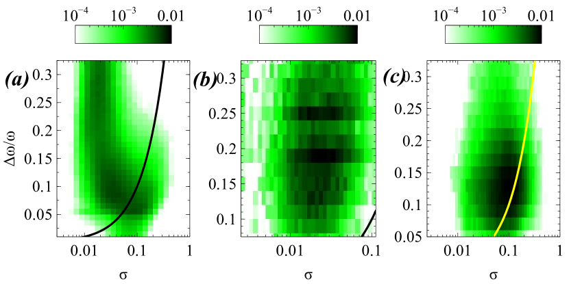
Figure 5: Distribution of statistics of field-aligned intense whistler-mode waves in ($\Delta\omega/\omega$, $\sigma$) parametric space where $\Delta\omega$ is the spectrum width, $\sigma=\sqrt{{\cal B}_{w}/B_{0}}\beta_{e}^{1/4}\left({\Omega_{0}/\omega-1}\right)^{-1/4}$ and $\beta_{e}$ is the electron plasma beta parameter (ratio of electron thermal pressure and background magnetic field pressure). Curves show the $\sigma=\Delta\omega/\omega$ threshold. Panel (a) shows statistics of field-aligned whistler-mode wave packets in the Earth’s outer radiation belt [see Zhang, Mourenas, Artemyev, Angelopoulos, Bortnik, Thorne, Kurth, Kletzing & Hospodarsky, 2019]; panel (b) shows statistics of whistler-mode waves observed in the plasma sheet, around injection regions Zhang, Angelopoulos, Artemyev & Liu [2018]; panel (c) shows statistics of very oblique whistler-mode waves observed in the outer radiation belt (we use THEMIS Angelopoulos [2008] electric field and magnetic field Bonnell et al. [2008]; Le Contel et al. [2008] wave measurements and the same criteria for wave identification as Li, Santolik, Bortnik, Thorne, Kletzing, Kurth & Hospodarsky [2016]).

Therefore, wave-particle resonant interactions should be considered under the assumption that electrons interact resonantly with individual intense waves. The corresponding Hamiltonian for wave particle interactions in dipole field can be written as (see Appendix A and [Albert, 1993; Albert et al., 2013; Vainchtein et al., 2018]):

$$H=m_{e}c^{2}\gamma-eU_{w}\left({I_{x},s}\right)\cos\left({\phi-{n_{r}}\psi}\right),\quad\gamma=\sqrt{1+\left({\frac{{p_{\parallel}}}{{m_{e}c}}}\right)^{2}+\frac{{2I_{x}\Omega_{0}\left(s\right)}}{{m_{e}c^{2}}}}$$ (2)

where $\Omega_{0}(s)=eB_{0}(s)/m_{e}c$ is the electron gyrofrequency, $(s,p_{\parallel})$ are conjugated field-aligned coordinate and momentum, $(\psi,I_{x})$ are conjugated gyrophase and magnetic moment ($I_{x}=(\gamma^{2}-1)m_{e}c^{2}\sin^{2}\alpha/\Omega_{0}$ and $\alpha$ is a local pitch-angle), ${n_{r}}=0,\pm 1,\pm 2,...$ is the resonance number. The resonance condition $\dot{\phi}={n_{r}}\dot{\psi}$, the wave phase definition $\dot{\phi}=k_{\parallel}(s)\dot{s}-\omega$, and Hamiltonian equations $\dot{\psi}=\partial H/\partial I_{x}=\Omega_{0}/\gamma$, $\dot{s}=\partial H/\partial p_{\parallel}=p_{\parallel}/m_{e}\gamma$ determine the resonant momentum $p_{\parallel}=p_{R}$:

$$p_{R}=m_{e}\frac{{\gamma\omega+{n_{r}}\Omega_{0}}}{{k_{\parallel}}}$$

The function $U_{w}$ is the generalized wave amplitude, including effects of whistler-mode dispersion (see Appendix A and [Albert, 1993; Artemyev, Neishtadt, Vasiliev & Mourenas, 2018]):

$$U_{w}=A_{w}\sum\limits_{{n_{r}}=-\infty}^{+\infty}{h^{({n_{r}})}}$$

and

$$h^{({n_{r}})}=\frac{{\rho\Omega_{0}}}{{2c\gamma}}\left({\left({C_{1}-\cos\theta}\right)J_{{n_{r}}-1}-\left({C_{1}+\cos\theta}\right)J_{{n_{r}}+1}}\right)-\left({\frac{{p_{\parallel}}}{{\gamma m_{e}c}}+C_{2}}\right)\sin\theta J_{{n_{r}}}$$

where $J_{{n_{r}}}$ are Bessel functions with argument $k_{\bot}\rho$, $\rho=\sqrt{2I_{x}/m_{e}\Omega_{0}}$, $\theta$ is the wave normal angle (wave number has two components: field-aligned $k_{\parallel}=k\cos\theta$ and transverse $k_{\perp}=k\sin\theta$). This equation for $u_{w}^{({n_{r}})}$ has been derived using the relations between wave magnetic and electric field components in a cold plasma Williams & Lyons [1974]; Tao & Bortnik [2010] and, thus, the coefficients $C_{1,2}$, given in Appendix A, depend only on wave characteristics. An important property of $C_{1}$ is that for $\theta=0$ (field-aligned propagation) it is equal to one, whereas $U_{w}^{({n_{r}})}=0$ for all ${n_{r}}$ except ${n_{r}}=-1$, for which we have $h^{(-1)}=\rho\Omega_{0}/c\gamma=\sqrt{2I_{x}\Omega_{0}/m_{e}c^{2}}$.

To describe the wave dispersion, $\omega=\omega(k,\theta)$, we again use the cold plasma approximation Stix [1962]:

$$N^{2}=\frac{1}{2}\frac{{(RL-PS)\sin^{2}\theta+2PS}}{{S\sin^{2}\theta+P\cos^{2}\theta}}+\frac{1}{2}\frac{{\sqrt{(RL-PS)^{2}\sin^{4}\theta+4P^{2}D^{2}\cos^{2}\theta}}}{{S\sin^{2}\theta+P\cos^{2}\theta}}$$

where $N=kc/\omega$ is the refractive index, and Stix coefficients are

$$R = 1-\sum\limits_{j}{\frac{{\Omega_{pj}^{2}}}{\omega}\frac{1}{{\omega+\Omega_{0j}}}},\quad L=1-\sum\limits_{j}{\frac{{\Omega_{pj}^{2}}}{\omega}\frac{1}{{\omega-\Omega_{0j}}}}$$

$$S = \frac{1}{2}(R+L),\quad D=\frac{1}{2}(R-L),\quad P=1-\sum\limits_{j}\Omega_{pj}^{2}/\omega^{2}$$

Here $\Omega_{0j}=e_{j}B/m_{j}c$ is the gyrofrequency for particles with a charge $j=e$ for electrons and $j=i$ or $j=p$ for ions or protons, $\Omega_{pj}=\sqrt{4\pi n_{0}e_{j}^{2}/m_{j}}$, $n_{0}$ is the background density ($n_{0}=n_{e}=n_{i}$). Note $e_{j}=-e$ for electrons and $e_{j}=e$ for protons.

A simplified form of this dispersion relation for a dense plasma is

$$\omega^{2}=\frac{{\Omega_{0}^{2}\cos^{2}\theta}}{{\left({1+(\Omega_{pe}/kc)^{2}}\right)^{2}}}+\frac{{\nu\Omega_{0}^{2}}}{{1+(\Omega_{pe}/kc)^{2}}}$$

where $\Omega_{pe}(s)\gg\Omega_{0}(s)$ is the electron plasma frequency, $\Omega_{0}=\Omega_{0e}$, and $\nu=m_{e}/m_{i}$, $m_{i}$ is the mass of the ion mixture (i.e., this is the proton mass for purely proton-electron plasma). For quasi-parallel wave propagation, $\theta\sim 0$, the last term in the simplified dispersion relation can be omitted:

$$\omega=\frac{{\Omega_{0}\cos\theta}}{{1+(\Omega_{pe}/kc)^{2}}}$$

Let us consider the Hamiltonian (2) under the assumption of constant wave frequency, $\omega=const$. Although this assumption is not applicable for the most intense whistler-mode chorus waves [Omura et al., 2008; Omura, 2021; Tao et al., 2021], it is quite useful to describe the basic properties of wave-particle interactions. In this case, the time dependence is included only as a linear term $\omega t$ in the wave phase $\phi$ and, therefore, we may remove this dependence (to obtain a conservative Hamiltonian) by changing the variables: from $(\psi,I_{x})$ to $(\zeta,I)$ where $\zeta={n_{r}}\psi+\phi$. The corresponding generating function is

$$W=\left({\phi-{n_{r}}\psi}\right)I+sp+\psi\tilde{I}_{x}$$

and the new Hamiltonian is

$${\cal H}_{I} = -\omega I+m_{e}c^{2}\gamma-eU_{w}\left({\tilde{I}_{x}-{n_{r}}I,s}\right)\cos\zeta$$

$$\gamma = \sqrt{1+\left({\frac{{p+k_{\parallel}I}}{{m_{e}c}}}\right)^{2}+\frac{{2\left({\tilde{I}_{x}-{n_{r}}I}\right)\Omega_{0}\left(s\right)}}{{m_{e}c^{2}}}}$$

where $p=p_{\parallel}-k_{\parallel}I$ is the new momentum conjugated to the new coordinate $\tilde{s}=s$ (keeping the $s$ notation), $I_{x}=\tilde{I}_{x}-{n_{r}}I$, and $I$ is conjugated to the new phase $\zeta$ [see, e.g., Artemyev, Neishtadt, Vasiliev & Mourenas, 2018].

The Hamiltonian (LABEL:eq:hamiltonian_const) does not depend on time, and thus ${\cal H}_{I}$=const, with the integral of electron motion

$$h=m_{e}c^{2}\gamma-\omega I$$ (4)

Note that $\tilde{I}_{x}$ is a constant, because ${\cal H}_{I}$ does not depend on $\psi$. For the case of Landau resonance, ${n_{r}}=0$, $\tilde{I}_{x}=I_{x}$, i.e., $I_{x}$ is conserved. Using this conservation law in Eq. (4) gives $h=\Omega_{eq}I_{x}=const$. For the first cyclotron resonance, ${n_{r}}=-1$, $\tilde{I}_{x}=I_{x}-I$ and can be set equal to zero, i.e. $I_{x}=I$. In this case, Eq. (4) can be written as:

$$h=m_{e}c^{2}\gamma-\omega I_{x}$$

The integral given by Eq.(4) describes trajectories, in the momentum space or in energy, pitch-angle space $(E,\alpha_{eq})$, along which wave-particle interactions are transporting electrons. Note that without such interactions, the energy $E=m_{e}c^{2}(\gamma-1)$ and equatorial pitch-angle $\alpha_{eq}={\rm asin}\left(2I_{x}\Omega_{eq}/(\gamma^{2}-1)\right)$ would be constants of motion. Figure 6 shows these trajectories (also called resonance curves; e.g., Walker [1993]) for the Landau (${n_{r}}=0$) and first cyclotron (${n_{r}}=-1$) resonances of electrons with whistler-mode waves. The main feature of the cyclotron resonance is that the resonance curves are almost parallel to the pitch-angle axis for small pitch-angles, and show energy increase with pitch-angle increase for larger pitch-angles. Thus, electrons transported to smaller pitch-angles (and finally into the loss-cone, thereby precipitating into the atmosphere) lose their energy, but around the loss-cone (at small pitch-angles) this transport occurs almost without energy change. The main feature of the Landau resonance is the large energy increase of electrons transported along the resonant curves toward smaller pitch-angles, i.e., electron precipitation due to the Landau resonance is accompanied by electron acceleration. In contrast to the cyclotron resonance, electron transport to higher pitch-angles via the Landau resonance is associated with electron energy loss. For the Landau resonance, the shape of resonance curves is dictated by magnetic moment conservation and does not depend on the wave frequency, whereas for the cyclotron resonance a smaller wave frequency means less energy change for the same pitch-angle change. At high energies for cyclotron resonance, the resonance curves show a change of direction: there, energy increase corresponds to pitch-angle decrease. This is the so-called turning acceleration effect [Omura et al., 2007], which occurs when $\gamma\omega/\Omega_{0}$ is larger than one and $d\gamma/d\alpha$ changes sign for large $\alpha$:

$$\frac{{d\gamma}}{{d\alpha}}=\frac{{\left({\omega/\Omega_{0}}\right)\left({\gamma^{2}-1}\right)\sin\alpha\cos\alpha}}{{1-\left({\omega\gamma/\Omega_{0}}\right)\sin^{2}\alpha}}$$

This equation is obtained by differentiation of Eq. (4) over $\alpha$. Note that $\gamma\omega/\Omega_{0}=1$ also separates cyclotron resonances with negative resonant momentum (waves and resonant particles are moving in opposite directions) and with positive resonant momentum (waves and resonant particles are moving in the same direction), $p_{R}=m_{e}\gamma\omega\left(1-\Omega_{0}/\gamma\omega\right)/k_{\parallel}$.

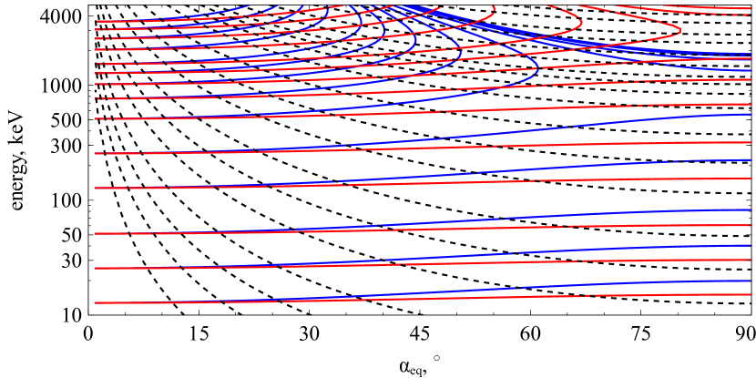
Figure 6: Resonance curves given by Eq. (4) for Landau (${n_{r}}=0$; dashed black line) and first cyclotron (${n_{r}}=-1$; solid red and blue lines) resonances. Two wave frequencies are shown: $\omega/\Omega_{eq}=0.15$ (red) and $\omega/\Omega_{eq}=0.35$ (blue).

The resonance curves in Fig. 6 show that for the same wave characteristics, electrons with different energies and pitch-angles (i.e., with different $h$ integrals of motion) can interact resonantly with a same monochromatic ($\omega=const$) wave. This is due to background magnetic field inhomogeneity: electrons bounce along magnetic field lines and have a different local pitch-angle $\alpha(s)={\rm asin}\left(\sin(\alpha_{eq})\sqrt{\Omega_{0}(s)/\Omega_{eq}}\right)$ at different magnetic latitudes (coordinate $s$). Accordingly, electrons with a fixed energy will be able to find a specific latitude where their pitch-angles will satisfy the resonance condition with a whistler-mode wave of fixed frequency. There are two important consequences of such magnetic field inhomogeneity: (1) a monochromatic wave may interact resonantly with electrons in a wide energy, pitch-angle range (in contrast to a homogeneous plasma, where only a wide wave spectrum may provide resonances over a wide energy, pitch-angle range), (2) electron bounce motion moves particles into the resonances and moves them out of the resonances, which are therefore of limited size in latitude, and of limited duration. This second effect actually replaces the limitation of the duration of the resonant interaction of electrons with whistler-mode waves that is due to the existence of a broad wave spectrum in classical quasi-linear models [see discussion in Karpman, 1974; Shklyar, 1981, 2011; Albert, 2001, 2010; Allanson et al., 2022].

2.1 Resonant interaction with monochromatic wave

Let us now consider the effects of a high wave amplitude on resonant particle dynamics for an arbitrary wave propagation angle. We start with the Hamiltonian (LABEL:eq:hamiltonian_const) and follow the standard procedure for analysis of resonant Hamiltonian systems [Neishtadt & Vasiliev, 2005; Neishtadt, 2014; Albert et al., 2013; Artemyev, Neishtadt, Vasiliev & Mourenas, 2018]. First, let us write the equation for the resonant condition, $\dot{\zeta}=0$

$$\dot{\zeta}=\frac{{\partial H_{I}}}{{\partial I}}\approx-\omega+m_{e}\frac{{{n_{r}}\Omega_{0}+k_{\parallel}\left({p+k_{\parallel}I}\right)}}{m_{e}\gamma}=0$$

where we omit the term

$$\sim\frac{{\partial eU_{w}}}{{\partial I}}\cos\zeta$$

that is proportional to the wave amplitude and should not be included into the definition of the resonance (see discussion of exceptions in Li et al. [2022] and discussion of the importance of this term in Appendix B).

Equation $\dot{\zeta}=0$ has a solution $I=I_{R}$, where

$$\frac{{k_{\parallel}I_{R}}}{{m_{e}c}}=-\frac{p}{{m_{e}c}}-\frac{{{n_{r}}\Omega_{0}}}{{k_{\parallel}c}}+\frac{1}{{\sqrt{N_{\parallel}^{2}-1}}}\sqrt{1+\frac{{2\tilde{I}_{x}\Omega_{0}}}{{m_{e}c^{2}}}-\left({\frac{{{n_{r}}\Omega_{0}}}{{k_{\parallel}c}}}\right)^{2}-2\frac{{{n_{r}}\Omega_{0}}}{{k_{\parallel}c}}\frac{p}{{m_{e}c}}}$$

where $N_{\parallel}=k_{\parallel}c/\omega$.

Expanding Hamiltonian (LABEL:eq:hamiltonian_const) around $I=I_{R}$, we obtain

$${\cal H}_{I} \approx \Lambda+\frac{1}{{2M}}\left({I-I_{R}}\right)^{2}+eU_{w}\left({I_{R},s}\right)\cos\zeta$$

$$\Lambda = -\omega I_{R}+m_{e}c^{2}\gamma_{R},\quad\gamma_{R}=\frac{{N_{\parallel}}}{{\sqrt{N_{\parallel}^{2}-1}}}\sqrt{1+\frac{{2\tilde{I}_{x}\Omega_{0}}}{{m_{e}c^{2}}}-\left({\frac{{{n_{r}}\Omega_{0}}}{{k_{\parallel}c}}}\right)^{2}-2\frac{{{n_{r}}\Omega_{0}}}{{k_{\parallel}c}}\frac{p}{{m_{e}c}}}$$

In Appendix A, we describe the variable change and the corresponding generating function: $(\zeta,I)\to(\zeta,P_{\zeta})$ where $P_{\zeta}=I-I_{R}$. After this change and an expansion relative to the resonance, the Hamiltonian ${\cal H}_{I}$ is separated into two parts. The first part

$$\Lambda=-\omega I_{R}(s,p)+m_{e}c^{2}\gamma_{R}(s,p)$$ (5)

describes the dynamics of slow variables, $(s,p)$. The second part

$${\cal H}_{\zeta}=\frac{1}{{2M}}P_{\zeta}^{2}+{\rm A}\zeta+{\rm B}\cos\zeta$$ (6)

describes the dynamics of fast variables $(\zeta,P_{\zeta})$, with coefficients depending on slow variables $(p,s)$. Coefficients $M$, ${\rm A}$, and ${\rm B}$ are derived in Appendix A for the general case of arbitrary wave propagation direction. For the first cyclotron resonance with field-aligned waves, these coefficients are

$${\rm A} = \left\{{\Lambda,I_{R}}\right\}_{s,p}\approx-\frac{{m_{e}c^{2}{\cal D}}}{{\gamma_{R}}}\frac{{N_{\parallel}^{2}}}{{N_{\parallel}^{2}-1}}\left({\left({\frac{{p_{\parallel,R}}}{{m_{e}c}}}\right)^{2}\frac{{\partial\ln N_{\parallel}}}{{\partial\ln\Omega_{0}}}+\frac{{\Omega_{0}}}{{\omega N_{\parallel}}}\frac{{p_{\parallel,R}}}{{m_{e}c}}-\frac{{\Omega_{0}I_{x,R}}}{{m_{e}c^{2}}}}\right)$$

$${\rm B} = eU_{w}\left({I_{R},s_{R}}\right),\quad M=\left({\frac{{\partial^{2}{\cal H}_{I}}}{{\partial I^{2}}}}\right)_{I_{R}}^{-1}=\frac{{m_{e}c^{2}}}{{\omega^{2}}}\frac{{\gamma_{R}}}{{N_{\parallel}^{2}-1}}$$

where $N_{\parallel}=k_{\parallel}c/\omega$, $p_{\parallel,R}=(\gamma_{R}-{n_{r}}\Omega_{0}/\omega)/N_{\parallel}$, ${\cal D}=c(\partial\ln\Omega_{0}/\partial s)/N_{\parallel}\omega\ll 1$ is a dimensionless factor of system inhomogeneity, and $s_{R}$ and $I_{x,R}$ are coordinate and momentum in the resonance.

These coefficients determine the character of wave-particle resonant interactions. Figure 7 shows the phase portrait for two regimes: $a=|{\rm B}/{\rm A}|<1$ and $a=|{\rm B}/{\rm A}|>1$, where

$$\frac{\rm B}{\rm A}=-\frac{{eU_{w}\left({I_{R},s_{R}}\right)\gamma_{R}}}{{m_{e}c^{2}{\cal D}}}\frac{{N_{\parallel}^{2}-1}}{{N_{\parallel}^{2}}}\left({\left({\frac{{p_{\parallel,R}}}{{m_{e}c}}}\right)^{2}\frac{{\partial\ln N_{\parallel}}}{{\partial\ln\Omega_{0}}}+\frac{{\Omega_{0}}}{{\omega N_{\parallel}}}\frac{{p_{\parallel,R}}}{{m_{e}c}}-\frac{{\Omega_{0}I_{x,R}}}{{m_{e}c^{2}}}}\right)^{-1}$$

For $a<1$ the phase portrait is filled by trajectories crossing the resonance, $\dot{\zeta}=P_{\zeta}/M=0$, only once. These are so-called transient trajectories, and as particles moving along these trajectories spend a quite limited time around the resonance, the wave field cannot significantly change their orbits. Such regime of wave-particle resonant interactions is principally similar to linear scattering, which is evaluated for unperturbed particle trajectories Karpman & Shklyar [1977]; Albert [2001].

For $a>1$ the phase portrait is divided into two domains: the internal domain is filled by closed trajectories with multiple resonance $\dot{\zeta}=0$ crossings, whereas the external domain is filled by open trajectories with a single resonance crossing, but particles on these trajectories need to move around the interval domain and thus spend much more time around the resonance in comparison with particles moving along transient trajectories. Particles inside the internal domain are called phase trapped and may spend a very long time in the resonance (oscillating around the resonance). Particles in the external domain will be scattered, but this scattering cannot be evaluated under the approximation of unperturbed trajectories. This nonlinear scattering is very different from the linear one, appropriate for transient trajectories. The entire problematic of nonlinear wave-particle interaction consists in developing an accurate description of such nonlinear scattering and phase trapping effects for a large ensemble of electrons.

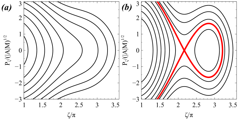
Figure 7: Phase portraits for Hamiltonian (6) for $a=|{\rm B}/{\rm A}|<1/2$ (a) and $a=|{\rm B}/{\rm A}|=2$ (b).

The factor $1/a$ is essentially the same parameter as the $S$-parameter used in previous studies of wave-particle resonant interactions by Helliwell [1967]; Omura et al. [2008, 2009] and as the $\tau/\alpha$-parameter used by Karpman et al. [1974, 1975]; Shklyar & Matsumoto [2009]; Shklyar [2011]. We can rewrite the expression for $a$ as

$$\frac{1}{a} = \frac{{m_{e}c^{2}}}{{eB_{w}\gamma_{R}}}\sqrt{\frac{{m_{e}c^{2}}}{{2\Omega_{0}I_{x}}}}\frac{k}{\omega}\frac{{N_{\parallel}}}{{N_{\parallel}^{2}-1}}\left({\frac{{\Omega_{0}I_{x}}}{{m_{e}c^{2}}}-\left({\frac{{p_{\parallel,R}}}{{m_{e}c}}}\right)^{2}\frac{{\partial\ln N_{a}}}{{\partial\ln\Omega_{0}}}-\frac{{\Omega_{0}}}{{\omega N_{a}}}\frac{{p_{\parallel,R}}}{{m_{e}c}}}\right)c\frac{{\partial\ln\Omega_{0}}}{{\partial s}}$$

$$= \frac{c}{{s^{\prime}_{0}\Omega_{w}\omega}}\frac{{\partial\Omega_{0}}}{{\partial s}}\frac{1}{{2\xi^{\prime}\delta^{\prime}}}\left({\frac{{\gamma_{R}\omega}}{{\Omega_{0}}}\left({\frac{{V^{\prime}_{\bot 0}}}{c}}\right)^{2}-2\gamma_{R}\frac{\omega}{{\Omega_{0}}}\left({\frac{{V^{\prime}_{R}}}{c}}\right)^{2}\frac{{\partial\ln N_{\parallel}}}{{\partial\ln\Omega_{0}}}-2\frac{{V^{\prime}_{R}V^{\prime}_{p}}}{{c^{2}}}}\right)$$

$$= \frac{c}{{s^{\prime}_{0}\Omega_{w}\omega}}\frac{{\partial\Omega_{0}}}{{\partial s}}\frac{1}{{2\xi^{\prime}\delta^{\prime}}}\left({\frac{{\gamma_{R}\omega}}{{\Omega_{0}}}\left({\frac{{V^{\prime}_{\bot 0}}}{c}}\right)^{2}-\left({2+\frac{\omega}{{\Omega_{0}}}\frac{{\Omega_{0}-\gamma_{R}\omega}}{{\Omega_{0}-\omega}}}\right)\frac{{V^{\prime}_{R}V^{\prime}_{p}}}{{c^{2}}}}\right)$$

where we used notation from [Omura et al., 2009]:

$$s^{\prime}_{0} = \frac{{N_{\parallel}^{2}-1}}{N_{\parallel}}\frac{{V_{\bot 0}}}{c},\quad\xi^{\prime}=\sqrt{N_{\parallel}^{2}-1},\quad\delta^{\prime}=\sqrt{1-N_{\parallel}^{-2}}$$

$$V^{\prime}_{R} = p_{\parallel,R}/m_{e}\gamma_{R},\quad V^{\prime}_{\bot 0}=c\sqrt{2I_{x}\Omega_{0}/m_{e}c^{2}}/\gamma_{R},\quad V^{\prime}_{p}=\omega/k=c/N_{\parallel}$$

and a simplified dispersion relation with constant plasma density (see Appendex A):

$$\frac{{\partial\ln N_{\parallel}}}{{\partial\ln\Omega_{0}}}=-\frac{1}{2}\frac{\omega}{{\Omega_{0}-\omega}}$$

In this form, $1/a$ fully coincides with $S$ given for $\partial\omega/\partial t=0$ by Eqs. (10)-(13) from Omura et al. [2009].

This parameter determines whether the wave field $\sim{\rm B}$ is sufficiently strong to overcome the inhomogeneity of the background magnetic field $\sim{\rm A}$. For $a>1$, the wave-particle resonant interaction is nonlinear, and this nonlinearity both changes the electron diffusion and introduces new effects of phase bunching and trapping. The parameter $a$ depends on background plasma and wave characteristics, but also on electron energy and pitch-angle. Figure 8 shows the probability distribution of $a>1$ for field-aligned whistler-mode waves in the outer radiation belt (this probability is displayed in $(E,\alpha_{eq})$ space). Medium to high pitch-angle electrons with not-too-high energies interact resonantly with waves close to the equator (where $\partial\Omega_{0}/\partial s$ is small), and this increases the probability of nonlinear interaction. Small pitch-angles and/or very high energy electrons interact resonantly with waves at high latitudes (farther from the equator), where the large $\partial\Omega_{0}/\partial s$ reduces the probability of nonlinear interaction. Note that the equation for $a$ has been derived from Hamiltonian (6), whereas this Hamiltonian would not work for very small pitch-angle particles having $I_{x}\Omega_{0}\sim eU_{w}$ (see details in Section 3.1 and Appendix B). In this limit of small pitch-angles, another criterion for nonlinear interactions can be derived Gan et al. [2024], which shows the possibility for such interactions.

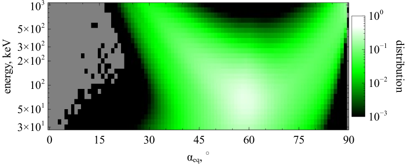
Figure 8: Probability distribution of $a>1$ (i.e., of nonlinear wave-particle interaction) for electrons and intense field-aligned whistler-mode waves in the outer radiation belt, for $L$-shell $\in[5,7]$. Dataset is from [Zhang, Mourenas, Artemyev, Angelopoulos, Bortnik, Thorne, Kurth, Kletzing & Hospodarsky, 2019].

2.2 Diffusion by monochromatic waves

To demonstrate how the inhomogeneity can affect wave-particle interactions, let us derive the electron diffusion rates in the simple case of a field-aligned whistler mode wave. Equations of motion for Hamiltonian (2) have the form:

$${\cal H}=mc^{2}\gamma-\sqrt{\frac{{2I_{x}\Omega_{0}}}{{m_{e}c^{2}}}}\frac{{eA_{w}}}{\gamma}\cos\left({\phi+\psi}\right),\quad\gamma=\sqrt{1+\left({\frac{{p_{\parallel}}}{{m_{e}c}}}\right)^{2}+\frac{{2I_{x}\Omega_{0}(z)}}{{m_{e}c^{2}}}}$$

and we can use $U_{w}=\sqrt{2I_{x}\Omega_{0}/m_{e}c^{2}}A_{w}/\gamma$.

Let us consider the approximation of a small wave amplitude $|{\rm A}|\gg|{\rm B}|$ at the resonance. Then, we can consider unperturbed ($U_{w}=0$) particle trajectories to determine the phase $\zeta$ variation around the resonance $t=t_{R}$, $\zeta_{R}=\zeta(t_{R})$. Expanding $\zeta$ around the resonance, we obtain

$$\zeta\approx\zeta_{R}+\frac{1}{2}\left({t-t_{R}}\right)^{2}\left.{\ddot{\zeta}}\right|_{t=t_{R}}$$

because $\dot{\zeta}|_{t=t_{R}}=0$. For Hamiltonian ${\cal H}_{\zeta}$ from Eqs. (6) $\ddot{\zeta}|_{t=t_{R}}$ can be expressed as

$$\ddot{\zeta}=\frac{{\dot{P}_{\zeta}}}{M}=\frac{{\left\{{\Lambda,I_{R}}\right\}}}{M}+\frac{{U_{w}}}{M}\cos\zeta\quad$$

Thus, for $|{\rm A}|\gg|{\rm B}|$ (i.e., $|{\Lambda,I_{R}}|\gg|eU_{w}|$) we have

$$\left.{\ddot{\zeta}}\right|_{t=t_{R}}=\frac{\rm A}{M}=\frac{{\left\{{\Lambda,I_{R}}\right\}}}{M}$$

Therefore, the $\Delta I$ change in the resonance is given by the time integral of $-\partial H_{I}/\partial\zeta$ and can be written as

$$\Delta I = eU_{w}\int\limits_{-\infty}^{+\infty}{\sin\zeta dt}=eU_{w}\int\limits_{-\infty}^{+\infty}{\sin\left({\zeta_{R}+\frac{1}{2}\left.{\ddot{\zeta}}\right|_{t=t_{R}}\left({t-t_{R}}\right)^{2}}\right)dt}$$ (7)

$$= 2eU_{w}\left({\left.{\frac{1}{2}\ddot{\zeta}}\right|_{t=t_{R}}}\right)^{-1/2}\left({\sin\zeta_{R}\int\limits_{0}^{+\infty}{\cos\left({q^{2}}\right)dq}+\cos\zeta_{R}\int\limits_{0}^{+\infty}{\sin\left({q^{2}}\right)dq}}\right)$$

$$= \sqrt{2\pi}eU_{w}\left({\left.{\frac{1}{2}\ddot{\zeta}}\right|_{t=t_{R}}}\right)^{-1/2}\sin\left({\zeta_{R}+\frac{\pi}{4}}\right)$$

where the $\pm\infty$ limits of integration correspond to the large $\Delta t\omega\gg 1$ approximation for the time $\Delta t$ of motion around the resonance, and we use the Fresnel integral equation

$$\int\limits_{0}^{+\infty}{\cos\left({q^{2}}\right)dq}=\int\limits_{0}^{+\infty}{\sin\left({q^{2}}\right)dq}=\sqrt{\frac{\pi}{8}}$$

The averaged momentum change is zero, $\langle\Delta I\rangle_{\zeta_{R}}=0$, and we have

$$\left\langle{\left({\Delta I}\right)^{2}}\right\rangle_{\zeta_{R}}=\frac{{\pi\left({eU_{w}}\right)^{2}}}{{\left.{\ddot{\zeta}}\right|_{t=t_{R}}}}=\pi\left({\frac{{m_{e}c^{2}}}{\omega}}\right)^{2}\frac{{B_{w}^{2}}}{{B_{0}^{2}}}\frac{{2I_{x}\Omega_{0}}}{{m_{e}c^{2}}}\frac{{\Omega_{0}^{2}}}{{\omega^{2}N_{\parallel}^{4}}}\frac{c}{{\delta v_{R}}}$$ (8)

where $\delta v_{R}$ is the effective resonance width:

$$\delta v_{R}=c\frac{{\partial\ln\Omega_{0}}}{{k_{\parallel}\partial s}}\left({\left({\frac{{p_{\parallel,R}}}{{m_{e}c}}}\right)^{2}\left({\frac{{\partial\ln N_{\parallel}}}{{\partial\ln\Omega_{0}}}+\frac{1}{2}}\right)+\frac{{\Omega_{0}}}{{\omega N_{\parallel}}}\frac{{p_{\parallel,R}}}{{m_{e}c}}+\frac{1}{2}\left({1-\gamma^{2}}\right)}\right).$$

In Eq. (8), all variables depending on $s$ should be evaluated at the resonance location.

Taking into account Eq. (4), the equation for $\left\langle{\left({\Delta\gamma}\right)^{2}}\right\rangle$ can be rewritten as

$$\left\langle{\left({\Delta\gamma}\right)^{2}}\right\rangle_{\zeta_{R}}=\left\langle{\left({\frac{{\omega\Delta I}}{{mc^{2}}}}\right)^{2}}\right\rangle_{\zeta_{R}}=\pi\frac{{B_{w}^{2}}}{{B_{0}^{2}}}\frac{{2I_{x}\Omega_{0}}}{{m_{e}c^{2}}}\frac{{\Omega_{0}^{2}}}{{\omega^{2}N^{4}}}\frac{c}{{\delta v_{R}}}$$

The conservation of magnetic moment $I_{x}=(\gamma^{2}-1)\sin^{2}\alpha_{eq}/2\Omega_{0}(0)$ provides an additional relation between energy $mc^{2}\gamma$ and pitch-angle $\alpha_{eq}$ changes:

$$\left.{\frac{{\partial\alpha_{eq}}}{{\partial\gamma}}}\right|_{I_{x}=const}=\frac{{\gamma\tan\alpha_{eq}}}{{\gamma^{2}-1}}$$

This relation allows the recalculation of $\left\langle{\left({\Delta\gamma}\right)^{2}}\right\rangle_{\zeta_{R}}$ to $\left\langle{\left({\Delta\alpha_{eq}}\right)^{2}}\right\rangle_{\zeta_{R}}$. Therefore, we may characterize wave-particle interactions by diffusion coefficients

$$D_{\gamma\gamma}=\frac{{\left\langle{\left({\Delta\gamma}\right)^{2}}\right\rangle_{\zeta_{R}}}}{{2\tau}},\quad D_{\alpha_{eq}\alpha_{eq}}=\frac{{\left\langle{\left({\Delta\alpha_{eq}}\right)^{2}}\right\rangle_{\zeta_{R}}}}{{2\tau}}=\left({\frac{{\gamma\tan\alpha_{eq}}}{{\gamma^{2}-1}}}\right)^{2}D_{\gamma\gamma}$$ (9)

where $\tau=\tau(\gamma,\alpha_{eq})$ is the time between two resonant interactions for a single resonance within half of a bounce period, $\tau=\tau_{bounce}/2$, and Eqs. (9) provide the bounce averaged energy and pitch-angle diffusion rates [see also Albert, 2010].

Note that Eq. (7) provides the $\Delta I$ change for unperturbed particle trajectories (i.e., when particle coordinate and velocity do not depend on $eU_{w}$) and, thus, $\Delta I\sim\int{eU_{w}\sin\zeta dt}$ with $\zeta=\zeta_{0}(t)$ does not depend on $eU_{w}$. The mean value of such a change is $\langle\Delta I\rangle=0$, whereas its variance is $\langle(\Delta I)^{2}\rangle\propto(eU_{w})^{2}$. The next order of particle trajectory perturbations should include terms linearly proportional to $eU_{w}$, and thus $\zeta=\zeta_{0}(t)+eU_{w}\cdot C\sin\left(\zeta_{0}(t)\right)$ where $C$ is a function of slow coordinates. At this next order, $\Delta I\sim\int{eU_{w}\sin\zeta dt}$ will contain two terms $\int{eU_{w}\sin\zeta_{0}dt}$ and $\sim\int{eU_{w}^{2}\sin^{2}\zeta dt}$, with a mean value $\langle\Delta I\rangle\propto(eU_{w})^{2}$ provided by the second term. Thus, to estimate $\langle\Delta I\rangle$ of the same order as $\langle(\Delta I)^{2}\rangle\propto(eU_{w})^{2}$, one needs to consider a second order perturbation of particle trajectories. The absence of a mean value $\langle\Delta I\rangle$ for the unperturbed trajectories does not mean that $\langle\Delta I\rangle=0$, but only implies that one has not $\langle\Delta I\rangle\propto eU_{w}$, but instead $\langle\Delta I\rangle\propto(eU_{w})^{2}$.

3 Nonlinear resonant characteristics

Let us describe the main characteristics of nonlinear resonant interactions. We start with the resonant energy change experienced by the particles crossing the resonance $\dot{\zeta}=0$, the so-called transient particles. Using Eq. (4), we can write $m_{e}c^{2}\Delta\gamma=\omega\Delta I$ where $\Delta I$ is given by integration of the Hamiltonian equation for Hamiltonian (LABEL:eq:hamiltonian_const):

$$\Delta I=2eU_{w}\int\limits_{-\infty}^{t_{R}}{\sin\zeta dt}$$

where $t_{R}$ is the time of resonance crossing ($\dot{\zeta}=0$). Using Hamiltonian (6) for $dt=d\zeta/\dot{\zeta}=Md\zeta/P_{\zeta}$, we obtain

$$\Delta I=2eU_{w}M\int\limits_{-\infty}^{\zeta_{R}}{\frac{{\sin\zeta}}{{P_{\zeta}}}d\zeta}=\int\limits_{-\infty}^{\zeta_{R}}{\frac{{eU_{w}\sqrt{2M}\sin\zeta d\zeta}}{{\sqrt{2\pi\xi{\rm A}-{\rm A}\zeta-{\rm B}\cos\zeta}}}}\\$$

where we introduce $\xi={\cal H}_{\zeta}/2\pi{\rm A}$, the energy of particles in the phase portrait from Fig. 7. Equation (3) can be written as $\Delta I=\Delta I_{0}F(\xi,a)$, where

$$\Delta I_{0}=\sqrt{2M\left|{\rm A}\right|}$$

and

$$F=\int\limits_{-\infty}^{\zeta_{R}}{\frac{{a\sin\zeta d\zeta}}{{\sqrt{2\pi\xi-\zeta-a\cos\zeta}}}}$$ (10)

The function $F$ is shown in Fig. 9(a). It is a periodic function of $\xi$ with the period $1$:

$$F(a,\xi+1) =\int\limits_{-\infty}^{\zeta_{R}}d\zeta\>\frac{\sqrt{a}\sin\zeta}{\sqrt{2\pi\xi+2\pi-\zeta-a\>\cos\zeta}}=\int\limits_{-\infty}^{\zeta_{R}-2\pi}d\tilde{\zeta}\>\frac{\sqrt{a}\sin\tilde{\zeta}}{\sqrt{2\pi\xi-\tilde{\zeta}-a\>\cos\tilde{\zeta}}}=$$

$$=\int\limits_{-\infty}^{\tilde{\zeta}_{R}}d\tilde{\zeta}\>\frac{\sqrt{a}\sin\tilde{\zeta}}{\sqrt{2\pi\xi-\tilde{\zeta}-a\>\cos\tilde{\zeta}}}=F(a,\xi)$$

For $a<1$, this periodic function is such that its average $\langle F(a,\xi)\rangle_{\xi\in[0,1)}$ is zero, whereas for $a>1$ the profile of $F$ becomes asymmetric relative to zero and $\langle f(a,\xi)\rangle_{\xi\in[0,1)}$ is finite (see Appendix A and Neishtadt [1975]). As function $F$ takes both positive and negative values, resonant electrons can increase and decrease their moment $I$, with $\Delta I\sim F$. The $\xi$-averaged $F$ is always non positive, and this determines the conventional description of electron resonant scattering (for $a>1$ and the first cyclotron resonance this scattering is called phase bunching, see Matsumoto & Omura [1981]; Omura & Matsumoto [1982]; Winglee [1985]) as a process with electron momentum (and energy) decrease [e.g., Albert, 2001]. However, for individual $\xi$ values (i.e., for specific values of electron resonant energy ${\cal H}_{\zeta}$) $\Delta I$ is positive, and this effect is called positive phase bunching and has been considered in [Albert et al., 2022; Vargas et al., 2023]. Although such positive phase bunching may be important for transient electron scattering by very intense whistler-mode wave packets [see discussion in Lundin & Shkliar, 1977; Inan et al., 1978], the overall electron ensemble dynamics can be described by $\xi$-averaged system characteristics that do not include positive phase bunching [Vargas et al., 2023].

The energy $\xi$ depends on initial particle gyrophase and can be considered as a random variable with uniform distribution within $[0,1]$ (see Fig. 8 in [Itin et al., 2000] and Fig. 5 in [Frantsuzov et al., 2023]). Therefore, to estimate the actual energy variation of transient particles we shall average the function $F$ over $\xi$ [see also Neishtadt, 2014; Artemyev, Neishtadt, Vainchtein, Vasiliev, Vasko & Zelenyi, 2018; Frantsuzov et al., 2023]:

$$\langle F\rangle_{\xi}=-\frac{1}{\pi}\int\limits_{\zeta_{-}}^{\zeta_{+}}{\sqrt{\zeta_{+}-\zeta+a\left({\cos\zeta_{+}-\cos\zeta}\right)}d\zeta}$$ (11)

This equation has been derived in Neishtadt [1975], and we repeat the derivations in Appendix A.

Equation (11) shows that $\langle\Delta I\rangle_{\xi}=\Delta I_{0}\langle F\rangle_{\xi}$ can be written as

$$\langle\Delta I\rangle_{\xi}=\sqrt{2M|{\rm A}|}\langle F\rangle_{\xi}$$ (12)

and is equal to $-{\cal S}/2\pi$, where ${\cal S}$ is the area surrounded by the separatrix in Fig. 7(b):

$${\cal S}={\sqrt{8M\left|{\rm A}\right|}}\int\limits_{\zeta_{-}}^{\zeta_{+}}{\sqrt{\zeta_{+}-\zeta+a\left({\cos\zeta_{+}-\cos\zeta}\right)}d\zeta},$$ (13)

Here the two $\zeta_{\pm}$ values are the coordinate of the saddle point ($\sin\zeta_{-}=1/a$) and a solution of $\zeta+a\cos\zeta=\zeta_{-}+a\cos\zeta_{-}$ equation, different from $\zeta_{-}$. From the definition of ${\cal S}$ it is clear that ${\cal S}=0$ for $a\leq 1$. The equality $\langle\Delta I\rangle_{\xi}=-{\cal S}/2\pi$ is an important property of the Hamiltonian system (6) that determines a balance between phase trapping and phase bunching processes [see Solovev & Shkliar, 1986; Itin et al., 2000; Artemyev, Neishtadt, Vasiliev & Mourenas, 2016]. A useful asymptotic expression of ${\cal S}$ is

$${\cal S}_{a\gg 1}\approx\sqrt{8M\left|B\right|}\int\limits_{0}^{2\pi}{\sqrt{1-\cos\zeta}d}\zeta=2^{5/2}\sqrt{8M\left|B\right|}=16\sqrt{M\left|B\right|}$$

where $\zeta_{-}\to 0$ and $\zeta_{+}\to 2\pi$. This asymptote shows that ${\cal S}$ scales with wave amplitude as ${\cal S}\propto\sqrt{|{\rm B}|}\propto\sqrt{U_{w}}\propto\sqrt{{\cal B}_{w}/B_{0}}$.

Figure 9(b) shows functions $\langle F(\xi,a)\rangle_{\xi}$, $\langle F^{2}(\xi,a)\rangle_{\xi}^{1/2}$, and $\sqrt{\langle F(\xi,a)^{2}\rangle_{\xi}-\langle F(\xi,a)\rangle_{\xi}^{2}}$ that describe the mean energy change, variance, and energy dispersion. Comparing Figs. 9(a) and (b), we see that although $F$ can be both positive and negative, the averaged $\langle F(\xi,a)\rangle_{\xi}$ is always positive (or zero, for $a<1$). Thus, individual particles may experience $\Delta I$ increase due to the phase bunching, but the $\xi$-averaged effect of such bunching corresponds to $\Delta I<0$. Such positive phase bunching ($\Delta I>0$) has been explained and investigated in Albert et al. [2022], whereas Vargas et al. [2023] demonstrated that positive bunching does change the overall dynamics of a charged particle ensemble, which can be fully described by the averaged $\langle F(\xi,a)\rangle_{\xi}$ function.

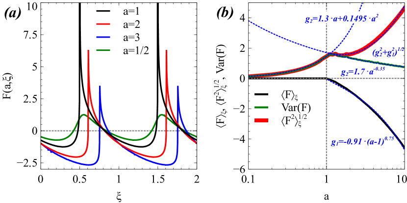
Figure 9: Panel (a) shows function $F(\xi,a)$ given by Eq. (10). Panel (b) shows functions $\langle F(\xi,a)\rangle_{\xi}$, $\langle F^{2}(\xi,a)\rangle_{\xi}^{1/2}$, and ${\rm Var}(F)=\sqrt{\langle F(\xi,a)^{2}\rangle_{\xi}-\langle F(\xi,a)\rangle_{\xi}^{2}}$. Blue dashed lines present fittings of the displayed functions.

Let us now consider particles experiencing phase trapping. In contrast with transient particles merely crossing the resonance $\dot{\zeta}=0$, trapped particles cross the separatrix (the curve demarcating open and closed trajectories in Fig. 7(b)), and their characteristic motion is qualitatively changed, i.e., they start oscillating around the resonance $\dot{\zeta}=0$. To estimate the amount of such particles, we shall compare the variation of the area surrounded by the separatrix, ${\cal S}$, and the total phase space flux ${\cal F}$ crossing the resonance:

$${\cal F}={\int\limits_{0}^{2\pi}{\dot{P}_{\zeta}d\zeta}}=2\pi{\rm A}$$

This comparison provides the so-called probability of trapping:

$$\Pi\approx\frac{{\left\{{{\cal S},\Lambda}\right\}}}{{\left|{\cal F}\right|+\left\{{{\cal S},\Lambda}\right\}/2}}=\frac{{2\left\{{{\cal S},\Lambda}\right\}}}{{4\pi\left|{\left\{{I_{R},\Lambda}\right\}}\right|+\left\{{{\cal S},\Lambda}\right\}}}$$ (14)

where $\dot{\cal S}=\{{\cal S},\Lambda\}$ and $\Pi=0$ for area decrease, $\dot{\cal S}<0$. If ${\cal S}$ changes slowly enough ( $\dot{\cal S}<4\pi|\{I_{R},\Lambda\}|$), which is the case in almost all systems under consideration, we can use the approximation

$$\Pi\approx\frac{{\left\{{{\cal S},\Lambda}\right\}}}{{2\pi\left|{\left\{{I_{R},\Lambda}\right\}}\right|}}$$ (15)

We note that ${I_{R},\Lambda}=\dot{I}_{R}$, and thus the probability of trapping can be rewritten as

$$\Pi\approx\frac{{\dot{\cal S}}}{{2\pi\dot{I}_{R}}}=\frac{1}{{2\pi}}\left.{\frac{{d{\cal S}}}{{dI}}}\right|_{I=I_{R}}$$

Taking into account that $\langle\Delta I\rangle_{\xi}=-{\cal S}/2\pi$, we obtain

$$\Pi\approx-\frac{{d\left\langle{\Delta I}\right\rangle_{\xi}}}{{dI}}$$

This equation provides a direct relationship between the probability of trapping and the average variation $\langle\Delta I\rangle_{\xi}$ due to nonlinear scattering.

The probability of trapping can be understood as the ratio of particles experiencing trapping for a single resonant interaction to the total number of particles crossing the resonance. For fixed system characteristics and $h$ constant, this probability depends only on the initial electron energy. Figure 10 shows examples of verification of Eq. (15) for the first cyclotron resonance with field-aligned waves and for the Landau resonance with very oblique waves [see more examples in Artemyev et al., 2012; Artemyev, Vasiliev, Mourenas, Agapitov, Krasnoselskikh, Boscher & Rolland, 2014; Artemyev, Vasiliev, Mourenas, Neishtadt, Agapitov & Krasnoselskikh, 2015; Vainchtein et al., 2018]. The usual scheme for an evaluation of the probability of trapping in numerical test particle simulations includes an integration of trajectories for a large particle ensemble with the same initial energy and pitch-angles, but random initial gyrophases. This ensemble passes through the resonance once and we can count the number of particles trapped into the resonance. The ratio of such trapped particles to the initial total number of particles in the ensemble will provide an estimate of the probability of trapping. Each colored circle in Fig. 10 has been obtained via such a scheme, applied to different particle (energy, pitch-angle) and system ($L$-shell, wave amplitude) parameters. This numerically evaluated probability of phase trapping is compared with the analytical formula of $\Pi$, confirming that Eq. (15) accurately describes the trapping probability. Note that we can resort to probabilities for the description of trapping, because in any realistic system the initial electron gyrophase is an unknown parameter. Therefore, we can average the system over this gyrophase to reduce its dimensionality, which leads to an inherently probabilistic description of trapping Neishtadt [1975]; Shklyar [1981].

Figure 10: Four sets of examples of numerical verification of the equation for the probability of trapping: curves show theoretical results from Eq. (15) and circles show results of test-particle simulations (a relative number of particles experiencing the phase trapping for a single resonant interaction). Panel (a) shows results for Landau resonance from Artemyev, Vasiliev, Mourenas, Agapitov & Krasnoselskikh [2013] (wave amplitudes are the same for black and blue curves, but a factor of $2$ larger for the red curve), panel (b) shows results for Landau resonance from Artemyev, Vasiliev, Mourenas, Agapitov, Krasnoselskikh, Boscher & Rolland [2014], panel (c) shows results for the cyclotron resonance from Artemyev, Vasiliev, Mourenas, Neishtadt, Agapitov & Krasnoselskikh [2015], and panel (d) shows results for the cyclotron resonance from Vainchtein et al. [2018]. Details of wave models and background magnetic field conditions can be found in the corresponding studies.

To evaluate the energy variation of an electron due to phase trapping, let us consider the motion of a trapped electrons. After crossing the separatrix in the phase portrait from Fig. 7(b), electrons start rotating around the resonance along closed trajectories. This rotation occurs with a frequency $\Omega_{tr}\sim\sqrt{{\rm B}/M}\propto({\cal B}_{w}/B_{0})^{1/2}\Omega_{0}$, whereas the phase portrait evolves with the rate of $(s,p)$ change, that is $\sim 2\pi/\tau_{b}\gg\Omega_{0}$ (the bounce period being the longest time scale in this system). Note that the resonance condition for whistler-mode waves assumes that $\Omega_{0}$ is of the same order as $k_{\parallel}\dot{s}\sim k_{\parallel}R/\tau_{b}$, where $R$ is the spatial scale of the background magnetic field inhomogeneity. On the other hand, the condition for nonlinear resonant interaction, $a>1$, assumes that $k_{\parallel}^{-1}\partial\ln\Omega_{0}/\partial s\sim 1/k_{\parallel}R$ is of the same order as the wave strength $\sim{\cal B}_{w}/B_{0}$, i.e. $k_{\parallel}R\sim B_{0}/{\cal B}_{w}$ and $\Omega_{0}\tau_{b}\sim B_{0}/{\cal B}_{w}\gg 1$. Thus, trapped electron oscillations around the resonance are much faster than the phase portrait evolution, $\Omega_{tr}\tau_{b}\propto({\cal B}_{w}/B_{0})^{1/2}\Omega_{0}\tau_{b}\propto({\cal B}_{w}/B_{0})^{-1/2}\gg 1$. Such a fast periodical motion should introduce an adiabatic invariant $I_{\zeta}=(2\pi)^{-1}\oint{P_{\zeta}d\zeta}$ [Landau & Lifshitz, 1960], which is equal to ${\cal S}_{tr}/2\pi$ evaluated at the time of trapping. Thus, trapped electrons move within the region surrounded by the separatrix, and at the time of trapping their invariant (area surrounded by their trajectories) is $I_{\zeta}={\cal S}_{tr}/2\pi$ with an increasing ${\cal S}_{tr}$. Electrons will stay trapped until ${\cal S}/2\pi$ becomes larger than $I_{\zeta}$. Accordingly, electrons will escape from the trapping regime when ${\cal S}={\cal S}_{tr}$ and ${\cal S}$ decreases. Illustration of this trapping/de-trapping dynamics is shown in Fig. 11.

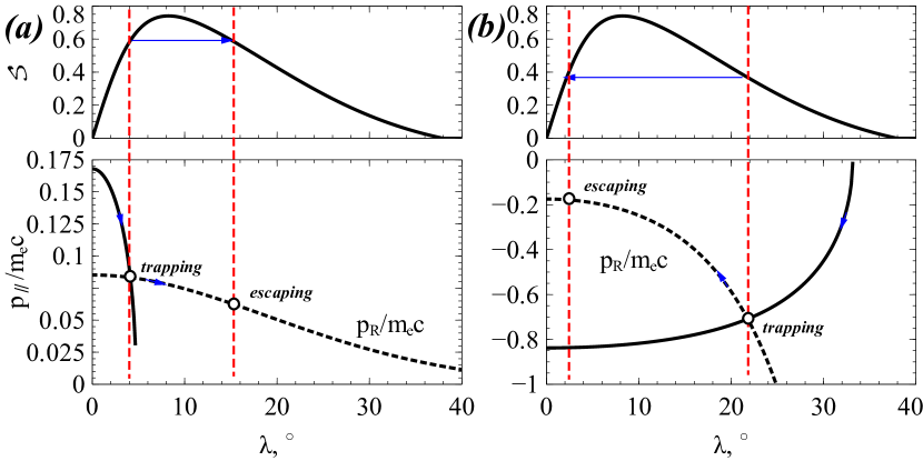
Figure 11: Schematic view of electron trapping/de-trapping (escape) for the Landau (a) and cyclotron (b) resonances. Top panels show typical profiles of area ${\cal S}(\lambda)$, and bottom panels show unperturbed electron trajectory $p_{\parallel}(\lambda)$ and resonant condition $p_{\parallel}=p_{R}(\lambda)$. Trapping and escape positions are shown by vertical red lines.

Figures 9-11 show that all nonlinear resonant effects are described by the ${\cal S}(I)$ (or ${\cal S}(\gamma)$) function: the energy variation of phase bunched particles is $\Delta\gamma=-\omega{\cal S}/2\pi m_{e}c^{2}$, the probability of phase trapping is $\Pi\approx(2\pi)^{-1}d{\cal S}/dI=(2\pi)^{-1}(d{\cal S}/d\gamma)\cdot(\omega/m_{e}c^{2})$, and the energy variation due to trapping is determined by the equation ${\cal S}(\gamma)={\cal S}\left(\gamma+\Delta\gamma_{tr}\right)$ [see also Artemyev, Neishtadt, Vasiliev & Mourenas, 2018]. Conversely, electron diffusion requires knowing $\langle F^{2}\rangle_{\xi}$, which cannot be expressed through the ${\cal S}=-2\pi\sqrt{2|{\rm A}|M}\langle F\rangle_{\xi}$ function, and should be evaluated separately. In the next section, we will use a quite universal property of ${\cal S}$ to construct a kinetic equation including the effects of nonlinear resonant interactions.

3.1 Small pitch-angle limit

There is one important limitation of system (6, 5): the factor $\sim{\cal B}_{w}\sqrt{2I\Omega_{0}}$ in the wave term is implicitly assumed to be constant within a typical time-scale of resonant interaction $\sim\Omega_{tr}^{-1}$. This assumption is valid as long as the phase variation $\dot{\zeta}$ is controlled by the $O({\cal B}_{w}/B_{0})$ term, while the term $\sim{\cal B}_{w}\sqrt{2\Omega_{0}/I}\sin\zeta$ remains a small correction. This assumption is naturally violated for sufficiently small $I$, when the term $\sim{\cal B}_{w}\sqrt{2\Omega_{0}/I}$ becomes important and the variation rate of $I$ becomes comparable to the $\zeta$ variation rate [Lundin & Shkliar, 1977]. A detailed description of this case can be found in [Albert et al., 2021; Artemyev, Neishtadt, Albert, Gan, Li & Ma, 2021] and in Appendix B, whereas multiple important effects of small $I$ (small $I_{x}$) on resonant electron motion are described in [Kitahara & Katoh, 2019; Grach & Demekhov, 2020; Gan et al., 2022]. Here, we only briefly discuss these effects.

Let us consider resonant nonlinear scattering of electrons with small $I_{x}=I$ and ${n_{r}}=-1$, and expand the Hamiltonian (LABEL:eq:hamiltonian_const) for small $I$:

$$\tilde{{\cal H}}_{I}\approx\Lambda_{0}+\frac{1}{{2M_{0}}}\left({I-I_{R}}\right)^{2}+\sqrt{\frac{{2I\Omega_{0}}}{{m_{e}c^{2}}}}\frac{{e{\cal B}_{w}}}{k}\cos\zeta$$

where $M_{0}=\partial^{2}{\cal H}_{I}/\partial I^{2}|_{I=0}$, $\Lambda_{0}={\cal H}_{I}|_{I=0}$, and $I_{R}$ is given in Appendix B. The main difference from the Hamiltonian expanded around the resonant $I_{R}$ is that wave amplitude in $\tilde{{\cal H}}$ depends on $I$. The Hamiltonian $\tilde{{\cal H}}_{I}$ describes fast $\zeta$ motion and slow $(s,p,I)$. An important property of this Hamiltonian is that for $I\sim({\cal B}_{w}/B_{0})^{2/3}$ the dynamics of $I$ becomes as fast as the dynamics of $\zeta$ and, thus, there is no time separation between $\zeta$ and $I$, which become fast variables. In Appendix B we show that the Hamiltonian of these fast variables is

$${\cal L}=\frac{1}{2}\left({\frac{1}{2}P^{2}+\frac{1}{2}q^{2}-Y_{R}}\right)^{2}+uq$$ (16)

where $P=({\cal B}_{w}/B_{0})^{-1/3}\sqrt{2I\Omega_{0}/m_{e}c^{2}}\sin\zeta$, $q=-({\cal B}_{w}/B_{0})^{-1/3}\sqrt{2I\Omega_{0}/m_{e}c^{2}}\cos\zeta$, $Y_{R}=({\cal B}_{w}/B_{0})^{-2/3}I_{R}\Omega_{0}/m_{e}c^{2}$, and $u$ is a normalization constant. The phase portrait of Hamiltonian (16) is shown in Fig. 12(c). Let us compare this phase portrait with phase portraits of the Hamiltonian expanded around $I_{R}$,

$${\cal H}_{I}=-\omega I_{R}+\gamma_{R}+\frac{1}{{2M}}\left({I-I_{R}}\right)^{2}+\sqrt{\frac{{2I_{R}\Omega_{0}}}{{m_{e}c^{2}}}}\frac{{e{\cal B}_{w}}}{{k}}\sin\zeta$$ (17)

The main difference between this Hamiltonian and the Hamiltonian from Eq. (16) is that the effective wave amplitude does not depend on $I$. The phase portrait of Hamiltonian (17) with frozen slow variables is shown in Fig. 12(a).

Instead of introducing $(q,P)$ coordinates, it is more convenient to introduce $P_{\zeta}=I-I_{R}$ and rewrite Hamiltonian (17) into Eq. (6). The phase portrait of Hamiltonian (6) with frozen slow variables is shown in Fig. 12(b). This is the classical portrait of the pendulum with torque with three main phase space regions: before resonance $P_{\zeta}=0$ crossing, particles are in $G_{1}$, and resonance crossing can result in trapping (particles appear in $G_{0}$) or scattering (particles appear in $G_{2}$). Therefore, there is a direct relation between three regions $G_{0,1,2}$ of Hamiltonian of (16) and Hamiltonian (6).

For the initial system given by Eq. (2) with ${n_{r}}=-1$ the phase bunching (transition from $G_{1}$ to $G_{2}$) always appears with $I_{x}$ decrease, and this effect is well seen in the phase portrait (c) of Fig. 12: the area ${\cal S}_{1}$ is always larger than the area ${\cal S}_{2}$. But when the initial invariant $I_{x}$ is sufficiently small, particles become trapped within region $G_{0}$ as soon as this region appears during particle motion along their trajectories. In phase portrait (c) of Fig. 12 this trapping means that the area surrounded by the particle trajectory $2\pi\oint{Pdq}\sim 2\pi\sqrt{2I\Omega_{0}/m_{e}c^{2}}$ is smaller than $S_{0}$ at the moment when $G_{0}$ appears. The threshold $I_{x}$ value is $2I_{x}\Omega_{0}/m_{e}c^{2}\sim({\cal B}_{w}/B_{0})^{2/3}$ (see Appendix B and Artemyev, Neishtadt, Albert, Gan, Li & Ma [2021]; Albert et al. [2021]).

This is the so-called autoresonance phenomena of 100% probability of trapping in resonant systems [see, e.g., Fajans & Frièdland, 2001; Friedland, 2009; Neishtadt et al., 2013; Neishtadt, 1975; Sinclair, 1972, and references therein]. Being trapped into $G_{0}$, particles can both increase or decrease their $I_{x}$ during the transition from $G_{0}$ to $G_{2}$: the $I_{x}$ change depends on the ratio of $S_{0}/S_{2}$ at the moment when $S_{0}$ becomes equal to $2\pi\oint{Pdq}$. For sufficiently small $2\pi\oint{Pdq}$ (small $I_{x}$), the ratio $S_{0}/S_{2}=2\pi\oint{Pdq}/S_{2}$ will be below one, and particles will increase their $I_{x}$ due to the resonant interaction. Formally, this interaction cannot be called bunching, because particles are trapped into $G_{0}$ from the beginning.

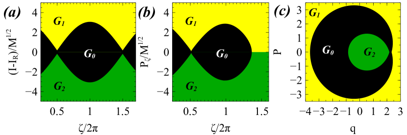
Figure 12: Comparison of phase portraits of (a) Hamiltonian (LABEL:eq:hamiltonian_const), (b) Hamiltonian (6), and (c) Hamiltonian (16).

4 Kinetic equation with nonlinear resonant effects

In this section, we use the function of ${\cal S}(\gamma)$ to derive a kinetic equation for the distribution function of electrons nonlinearly interacting resonantly with whistler-mode waves for a constant $h$ given by Eq. (4). Let us start with the simplified situation of a constant bounce period $\partial\tau_{b}/\partial\gamma=0$. We separate the $\hat{K}$ kernel into two parts: one part describing diffusion and the phase bunching effect $\hat{K}_{bc}$ and another part describing the trapping effect $\hat{K}_{tr}$. Using the approximation of small energy change due to bunching, we expand $\hat{K}_{bc}$ as

$$\int\limits_{0}^{\infty}{\hat{K}_{bc}(\gamma,\gamma^{\prime})f(\gamma^{\prime})d\gamma^{\prime}}=\frac{\partial}{{\partial\gamma}}\left({D_{\gamma\gamma}\frac{{\partial f}}{{\partial\gamma}}}\right)-\frac{\partial}{{\partial\gamma}}\left({V_{\gamma}f}\right)$$

Note that there are two main contributions to the particle drift term $V_{\gamma}$: the gradient of the diffusion rate, $V_{\gamma}\propto\partial D_{\gamma\gamma}/\partial\gamma\propto({\cal B}_{w}/B_{0})^{2}$, and nonlinear scattering (phase bunching effect), $V_{\gamma}\propto{\cal S}\propto({\cal B}_{w}/B_{0})^{1/2}$. The first term determines the divergence-free condition for the Fokker-Planck diffusion equation and is taken into account in the form of a $\propto D_{\gamma\gamma}$ operator Lieberman & Lichtenberg [1973]; Sagdeev et al. [1988]. Thus, in the equation for $\hat{K}_{bc}$ we may include only the second term $V_{\gamma}\propto({\cal B}_{w}/B_{0})^{1/2}$, which is much larger than the first one, because ${\cal B}_{w}/B_{0}\ll 1$.

For the trapping kernel, we use the following formulation:

$$\int\limits_{0}^{\infty}{\hat{K}_{tr+}\left({\left.\gamma\right|\gamma^{\prime}}\right)f\left({\gamma^{\prime}}\right)d\gamma^{\prime}}-\int\limits_{0}^{\infty}{\hat{K}_{tr-}\left({\left.{\gamma^{\prime}}\right|\gamma}\right)f\left(\gamma\right)d\gamma^{\prime}}$$

where the second term describes particle transport from the energy of trapping, $\gamma$, and the first term describes particle transport toward the energy of escape from the resonance, $\gamma$, from the energy of trapping, $\gamma^{\prime}$, given by ${\cal S}(\gamma^{\prime})={\cal S}(\gamma)$. Substituting $K_{bn}$ and $K_{tr}$ into the Smoluchowski equation (1), we obtain

$$\frac{{\partial f}}{{\partial t}} = \frac{\partial}{{\partial\gamma}}\left({D_{\gamma\gamma}\frac{{\partial f}}{{\partial\gamma}}}\right)-\frac{\partial}{{\partial\gamma}}\left({V_{\gamma}f}\right)$$

$$+ \int\limits_{0}^{\infty}{\hat{K}_{tr+}\left({\left.\gamma\right|\gamma^{\prime}}\right)f\left({\gamma^{\prime}}\right)d\gamma^{\prime}}-\int\limits_{0}^{\infty}{\hat{K}_{tr-}\left({\left.{\gamma^{\prime}}\right|\gamma}\right)f\left(\gamma\right)d\gamma^{\prime}}$$

The term responsible for particle transport from the energy of trapping, $\gamma$, can be written as

$$\int\limits_{0}^{\infty}{\hat{K}_{tr-}\left({\left.{\gamma^{\prime}}\right|\gamma}\right)f\left(\gamma\right)d\gamma^{\prime}}=\int\limits_{0}^{\infty}{\frac{\Pi\left(\gamma\right)}{\tau_{b}}\delta\left({\gamma-\gamma^{\prime}}\right)f\left(\gamma\right)d\gamma^{\prime}}=\frac{\Pi(\gamma)}{\tau_{b}}f(\gamma)\left(1-\Theta\right)$$

where

$$\Theta\left(\gamma\right){\rm=}\left\{{\begin{array}[]{*{20}c}{{\rm 0,}}&{dS/d\gamma<0}\\ {{\rm 1,}}&{dS/d\gamma>0}\\ \end{array}}\right.$$ (18)

The term responsible for particle transport from the energy $\gamma^{\prime}$ into the energy of escape, $\gamma$, can be written as

$$\int\limits_{0}^{\infty}{\hat{K}_{tr+}\left({\left.\gamma\right|\gamma^{\prime}}\right)f\left({\gamma^{\prime}}\right)d\gamma^{\prime}} = \int\limits_{0}^{\infty}{\Pi\left({\gamma^{\prime}}\right)\delta\left({\gamma-{\rm T}\left({\gamma^{\prime}}\right)}\right)f\left({\gamma^{\prime}}\right)d\gamma^{\prime}}$$

$$= \frac{\Pi\left({\gamma^{*}}\right)}{\tau_{b}}\left|{\frac{{d{\rm T}\left({\gamma^{*}}\right)}}{{d\gamma^{*}}}}\right|^{-1}f\left({\gamma^{*}}\right)$$

where ${\rm T}(\gamma^{*})=\gamma$ is the solution of the equation ${\cal S}(\gamma^{*})={\cal S}(\gamma)$. Note that Eq. (4) provides a linear relation between electron energy $\gamma$ and momentum $I$: $d\gamma/dI=\omega/m_{e}c^{2}=const$. This relation allows us to use the equation $d\gamma^{*}/d\gamma=dI^{*}/dI$ to write:

$$\frac{{dT\left({\gamma^{*}}\right)}}{{d\gamma^{*}}}=\frac{{d\gamma}}{{d\gamma^{*}}}=\frac{{dI}}{{dI^{*}}}=\frac{{dS\left({I^{*}}\right)/dI^{*}}}{{dS\left(I\right)/dI}}=-\frac{{\Pi\left({I^{*}}\right)/\tau_{b}}}{{dS\left(I\right)/dI}}=-\frac{{\Pi\left({\gamma^{*}}\right)/\tau_{b}}}{{dV_{\gamma}\left(\gamma\right)/d\gamma}}$$

Thus, for $\hat{K}_{tr+}$ we obtain for $\Theta=1$

$$\int\limits_{0}^{\infty}{K_{tr+}\left({\left.\gamma\right|\gamma^{\prime}}\right)f\left({\gamma^{\prime}}\right)d\gamma^{\prime}}=\frac{{dS\left(\gamma\right)}}{{d\gamma}}f\left({\gamma^{*}}\right)$$

Therefore, combining all these terms in the equation for $\partial f/\partial t$, we obtain:

$$\frac{{\partial f}}{{\partial t}}=\frac{\partial}{{\partial\gamma}}\left({D_{\gamma\gamma}\frac{{\partial f}}{{\partial\gamma}}}\right)-\frac{\partial}{{\partial\gamma}}\left({V_{\gamma}f}\right)+\frac{{dV_{\gamma}\left(\gamma\right)}}{{d\gamma}}f\left({\gamma^{*}}\right)\Theta-\frac{{\Pi\left(\gamma\right)}}{{\tau_{b}}}f\left(\gamma\right)\left(1-\Theta\right)$$ (19)

Taking into account that $\Pi=(2\pi)^{-1}(d{\cal S}/dI)=-dV_{\gamma}/d\gamma$, we can rewrite Eq.(19) as:

$$\frac{{\partial f}}{{\partial t}}=\frac{\partial}{{\partial\gamma}}\left({D_{\gamma\gamma}\frac{{\partial f}}{{\partial\gamma}}}\right)-V_{\gamma}\frac{\partial f}{{\partial\gamma}}+\frac{{dV\left(\gamma\right)}}{{d\gamma}}\left(f\left({\gamma^{*}}\right)-f\left({\gamma}\right)\right)\Theta$$

This is a basic formulation of a kinetic equation describing electron distribution dynamics due to multiple nonlinear resonant interactions. The numerical solution of this equation has been verified by comparisons with test particle simulations in Artemyev, Neishtadt, Vasiliev & Mourenas [2016]; Artemyev et al. [2017b]; Leoncini et al. [2018]. Figure 13 shows two examples of such verifications. We use two different initial conditions for the $f(\gamma)$ function and solve Eq. (19) within the energy range of ${\cal S}\neq 0$, i.e., we consider electron dynamics only within the energy range of nonlinear resonant interactions, $\gamma\in[\gamma_{\min},\gamma_{\max}]$. The diffusion rate $D_{\gamma\gamma}$ does not necessary vanish at $\gamma_{\min,\max}$ and particles can diffusively move in/out of the energy range of nonlinear resonant interactions. Thus, to verify Eq. (19) within the range $\gamma\in[\gamma_{\min},\gamma_{\max}]$ we numerically modify $D_{\gamma\gamma}\to D_{\gamma\gamma}\cdot 4\left(\gamma-\gamma_{\min}\right)^{2}\left(\gamma_{\max}-\gamma\right)^{2}/\left(\gamma_{\max}-\gamma_{\min}\right)^{4}$, to guarantee that electrons will not leave the range $\gamma\in[\gamma_{\min},\gamma_{\max}]$ of nonlinear resonant interactions. We also numerically integrate $10^{6}$ test particle trajectories described by the Hamiltonian (2).

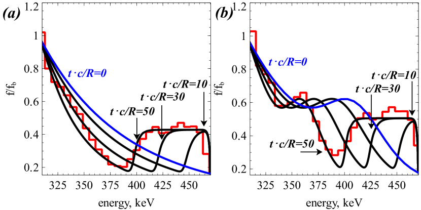
Figure 13: Solutions of Eq. (19) for two initial conditions (shown in blue). The function $f$ is normalized to its initial value at the left boundary, $f_{b}$. Results are shown at three different times, and the solution for $tc/R=50$ is compared with results of test particle simulations (red) with $10^{6}$ trajectories. Solutions are obtained for $h/m_{e}c^{2}=1.454$ (this value of $h$ corresponds to, e.g., an equatorial pitch-angle $\alpha_{eq}=45^{\circ}$ for 300 keV electron energy). We use a curvature-free dipole magnetic field [Bell, 1984] at $L$-shell$=4.5$. The whistler-mode wave frequency is $0.35$ times the electron cyclotron frequency at the equator, and the plasma frequency is $4.5$ times the electron cyclotron frequency at the equator. Wave amplitude is $300$ pT. The distribution of the wave amplitude along magnetic field lines is modeled by the empirical function $\tanh((\lambda/\delta\lambda_{1})^{2})\exp(-(\lambda/\delta\lambda_{2})^{2})$ with $\delta\lambda_{1}=2^{\circ}$, $\delta\lambda_{2}=20^{\circ}$. This empirical function fits the typically observed whistler-mode wave intensity distribution Agapitov et al. [2013].

The solutions shown in Fig. 13(a) start with a power law distribution $f\sim\gamma^{-3}$. Phase trapping forms an accelerated population of electrons at large energies, and with time this population drifts to smaller energies due to the phase bunching. The fine balance of bunching speed and trapping probability prevents an accumulation of electrons in the region where electrons are released from trapping acceleration: the new accelerated population only replaces a previously accelerated population moved to smaller energy, and the electron population at large energy does not increase in magnitude but occupies a larger energy range as time goes on. At the time $50R/c$, corresponding to about fifty bounce periods with a single resonant interaction during each period, we compare the solution of Eq. (19) with test particle simulation results: the corresponding red and black curves are quite close, demonstrating that the kinetic equation describes well the dynamics of the electron energy distribution.

The solutions shown in Fig. 13(b) start with a distribution having a small maximum at intermediate energies and a plateau. The resonant dynamics of the electron energy distribution includes the same components shown in Fig. 13(a): formation of an accelerated population due to phase trapping and the following drift of this population to smaller energies due to phase bunching. This dynamics is supplemented by the evolution of the maximum initially present at intermediate energies: due to an absence of phase trapping at these energies, this maximum merely drifts toward smaller energies via phase bunching. The enhanced electron population at smaller energies (due to the initial plateau) provides more particles for trapping acceleration, and the accelerated population in Fig. 13(b) has a larger magnitude in comparison with the population shown in Fig. 13(a). The comparison of solution of Eq. (19) with results of test particle simulations (at time $50R/c$) confirms that the kinetic equation describes correctly the dynamics of the electron energy distribution.

We note that in the case of test particle simulations, we cannot perform the modification of the diffusion coefficient that prevents particle escape from the energy range of nonlinear wave-particle interactions in the numerical solution of Eq. (19). Thus, to perform fair comparisons between test particle simulations and solutions of Eq. (19), we rerun each particle escaping $\gamma\in[\gamma_{\min},\gamma_{\max}]$ and save the total number of particles within this energy range. The diffusion $D_{\gamma\gamma}$ changes the electron distribution much slower than nonlinear resonant phase trapping and bunching, and such a weak effect of diffusion may help the comparison of test particle simulation results with solutions of Eq. (19), despite the different descriptions of diffusive scattering in the frame of these two approaches (due to $D_{\gamma\gamma}$ modification in the kinetic equation).

4.1 Boundary conditions

The profile ${\cal S}(\gamma)$ determines all the main terms of the kinetic equation (19) and, therefore, the properties of ${\cal S}(\gamma)$ are very important for understanding the solution of this equation. The important characteristic of ${\cal S}(\gamma)$ is its asymptotic behavior near zero values. Depending on the specific distribution of wave electromagnetic field (the term $\sim B_{w}$ in Eq. (2)0, there are different numbers of zeros of ${\cal S}(\gamma)$, but the simplest case corresponds to the cyclotron resonance with field-aligned whistler-mode waves when the term $\sim{\cal B}_{w}$ varies monotonically along the magnetic latitude. Note that for a conserved invariant $h$ from Eq. (4), the resonant energy $\gamma$ is a linear function of $I=I_{x}$ and a monotonic function of magnetic latitude $\lambda$ (or coordinate $s$). Figure 14(a) shows examples of latitudinal profiles of resonant energy for different $h$ values.

Near the equatorial plane, ${\cal S}(\gamma)$ should drop to zero because ${\cal B}_{w}\to 0$ in the wave source region, and thus $a\propto{\cal B}_{w}$ is less than one [see Shklyar, 2017, 2021; Shklyar & Luzhkovskiy, 2023, for descriptions of alternative ${\cal B}_{w}$ profiles for whistler-mode waves generated by lightning in the ionosphere and propagating from high latitudes to the equator]. At high latitudes, the gradient $\partial\Omega_{0}/\partial s$ becomes quite large and thus $a\propto\left(\partial\Omega_{0}/\partial s\right)^{-1}$ becomes less than one. Thus, for sufficiently large ${\cal B}_{w}$ we find that ${\cal S}$ is above zero between the equatorial plane and some high-latitude location. Let us consider the behavior of ${\cal S}$ around these two zeros, where $a\to 1$. First, we expand Hamiltonian (6) as [see Artemyev, Neishtadt & Vasiliev, 2019; Artemyev, Neishtadt, Vasiliev & Mourenas, 2021]:

$${\cal H}_{\zeta}=\frac{1}{2M}P_{\zeta}^{2}+{\rm B}\cdot\left({\frac{1}{a}\zeta+\cos\zeta}\right)\approx\frac{1}{2M}P_{\zeta}^{2}-{\rm B}\cdot\left({\left({1-\frac{1}{a}}\right)\zeta-\frac{1}{6}\zeta^{3}}\right)$$ (20)

where we expand $\cos\zeta$ around $\zeta=\pi/2$ and shift $\zeta\to\zeta-\pi/2$. The profile of potential energy  $U/{\rm B}=-\left(1-a^{-1}\right)\zeta+\zeta^{3}/6$ for this Hamiltonian is shown in Fig. 14(b): potential energy has a local minimum in the interval $(\zeta_{-},\zeta_{+})$. The corresponding area surrounded by the separatrix takes the form

$${\cal S}_{a\approx 1} = \sqrt{8M|{\rm B}|}\int\limits_{\zeta_{-}}^{\zeta_{+}}{\sqrt{\left({1-a^{-1}}\right)\left({\zeta-\zeta_{-}}\right)-\frac{1}{6}\left({\zeta^{3}-\zeta_{-}^{3}}\right)}d\zeta}$$

$$= \sqrt{8M|{\rm B}|}\left({1-a^{-1}}\right)^{5/4}\int\limits_{\tilde{\zeta}_{-}}^{\tilde{\zeta}_{+}}{\sqrt{\left({\tilde{\zeta}-\tilde{\zeta}_{-}}\right)-\frac{1}{6}\left({\tilde{\zeta}^{3}-\tilde{\zeta}_{-}^{3}}\right)}d\tilde{\zeta}}$$

$$= \sqrt{8M|{\rm B}|}\left({1-a^{-1}}\right)^{5/4}\frac{{12\cdot 3^{3/4}}}{5}=\frac{{12\cdot 3^{3/4}}}{5}\sqrt{8M\frac{|{\rm A}|^{5/2}}{|{\rm B}|^{3/2}}}\left({a-1}\right)^{5/4}$$

where $\tilde{\zeta}=\zeta/\left(a^{-1}-1\right)^{1/2}$. This equation provides the asymptotic variation of ${\cal S}$ for $a\to 1$, and we can rewrite this asymptote as a function of the resonant energy. Indeed, $a$ is a function of $s$, and for a conserved $h$ given by Eq. (4) there is a profile of resonant energy $\gamma(s)$, see Fig. 14(a). Therefore, we can write $a=a(\gamma)$ and then expand $a$ around the energy $\gamma_{b}$ corresponding to $a=1$ and ${\cal S}=0$: $a\approx 1+C\cdot(\gamma-\gamma_{b})$, where $C=const$. Substituting this expansion into equation ${\cal S}_{a\approx 1}$, we obtain

$${\cal S}_{a\approx 1}\propto\left|\gamma-\gamma_{b}\right|^{5/4}$$

Note that ${\cal S}\neq 0$ within some $\gamma\in[\gamma_{\min},\gamma_{\max}]$ domain, and we should have an asymptotic form ${\cal S}\propto|\gamma-\gamma_{\min,\max}|^{5/4}$ at both boundaries. This asymptotic form of ${\cal S}$ around $a\approx 1$ shows that $\Pi\propto d{\cal S}/d\gamma\propto|\gamma-\gamma_{b}|^{1/4}\to 0$ at the energy boundary, i.e., both drift $V\propto{\cal S}$ and probability of trapping $\Pi$ drop to zero at the boundary.

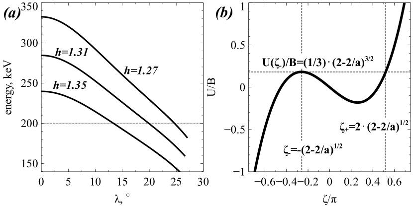
Figure 14: (a) Resonant energy $(\gamma-1)m_{e}c^{2}$ as a function of magnetic latitude for first cyclotron resonance with field-aligned waves ($\omega/\Omega_{eq}=0.35$, $L=6$) for several $h$ (equatorial pitch-angle $60^{\circ}$, $45^{\circ}$, and $30^{\circ}$ for $200$keV electron) values. (b) Profile of of potential energy $U/B=\zeta^{3}/6-\zeta(1-a^{-1})$ for Hamiltonian (20).

The equation for ${\cal S}_{a\approx 1}$ determines the ${\cal S}$ profile around the zeros, and can be adopted to describe systems with intrinsically small ${\cal S}$. The most natural example of such systems is a system with wave-packets. The corresponding schematic is provided in Fig. 15(a). The plane wave $\sim\sin(\zeta)$ is a very simplified approximation of much more complicated and realistic situations, where the wave field often consists of a series of wave-packets [Zhang, Mourenas, Artemyev, Angelopoulos, Bortnik, Thorne, Kurth, Kletzing & Hospodarsky, 2019; Zhang, Agapitov, Artemyev, Mourenas, Angelopoulos, Kurth, Bonnell & Hospodarsky, 2020]. Each packet has a finite length, and small-scale packets will correspond to a small latitudinal range of ${\cal S}\neq 0$, i.e., the $a\approx 1$ regime will be applicable for the entire range of energies with ${\cal S}\neq 0$. Then, ${\cal S}$ can be approximated as

$${\cal S}_{small}=S_{0}\cdot\left(\gamma_{\max}-\gamma\right)^{5/4}\left(\gamma-\gamma_{\min}\right)^{5/4}$$

where $S_{0}$ is the magnitude of ${\cal S}$ and $\gamma_{\max,\min}$ are boundary values of energies where $a=1$. Using changes of variables, $x=2\gamma/(\gamma_{\max}-\gamma_{\min})-(\gamma_{\max}+\gamma_{\min})/(\gamma_{\max}-\gamma_{\min})$ and $S_{0}\to S_{0}\cdot\left((\gamma_{\max}-\gamma_{\min})/2\right)^{5/2}$, we can write

$${\cal S}_{small}=S_{0}(1-x^{2})^{5/4}$$ (21)

with the equation for the probability of trapping $\Pi=d{\cal S}_{small}/dx=-(5/2)\cdot xS_{0}(1-x^{2})^{1/4}$. Equation (21) provides a very convenient and useful model for investigating the properties of systems with nonlinear wave particle resonant interactions. This equation works as long as the area is sufficiently large that $\Delta x_{tr}\gg\Delta x_{bn}\sim S_{0}$ (see scheme in Fig. 15(b)), and with the decrease of $(\gamma_{\max}-\gamma_{\min})$ (with increase of $S_{0}$) this equation becomes inapplicable (see Artemyev, Neishtadt, Vasiliev & Mourenas [2021] and Appendix C).

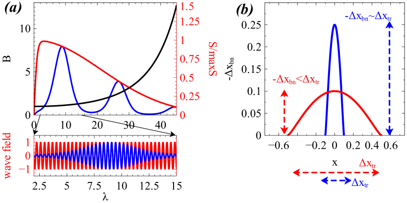
Figure 15: Panel (a) shows a schematic view of ${\cal S}$ profiles for plane wave (red) and wave-packet (blue). Panel (b) shows the difference of $S(x)/2\pi=-\Delta x_{bn}(x)$ profiles for a long wave-packet having $\Delta x_{tr}\gg|\Delta x_{bn}|$ and for short wave-packets having $\Delta x_{tr}\sim|\Delta x_{bn}|$

4.2 Asymptotic solutions

Let us consider the asymptote of the solution of Eq. (19) for $t\to\infty$ [see details in Artemyev, Neishtadt & Vasiliev, 2019]. We use the normalized variable $x=2\gamma/(\gamma_{\max}-\gamma_{\min})-(\gamma_{\max}+\gamma_{\min})/(\gamma_{\max}-\gamma_{\min})$ and rewrite this equation as

$$\frac{{\partial f}}{{\partial t}}=\left\{{\begin{array}[]{*{20}c}{-V\left(x\right)\frac{{\partial f}}{{\partial x}}+\frac{1}{2}\frac{\partial}{{\partial x}}\left({D\left(x\right)\frac{\partial}{{\partial x}}}\right),}&{x\leq 0}\\ {-V\left(x\right)\frac{{\partial f}}{{\partial x}}-\frac{{dV\left(x\right)}}{{dx}}\left({f-f^{\prime}}\right)+\frac{1}{2}\frac{\partial}{{\partial x}}\left({D\left(x\right)\frac{\partial}{{\partial x}}}\right),}&{x\geq 0}\\ \end{array}}\right.$$ (22)

where $V(x)=V_{0}(1-x^{2})^{5/4}$ for $x\in[-1,1]$, $f^{*}=f(x^{*})$ and $x^{*}=-x$. This equation, as well as Eq. (19), conserves the total number of particles:

$$\frac{d}{{dt}}\int\limits_{-1}^{1}{f\left({x,t}\right)dx}=\int\limits_{-1}^{1}{\frac{{\partial f\left({x,t}\right)}}{{\partial t}}dx}=\int\limits_{-1}^{1}{\frac{1}{2}\frac{\partial}{{\partial x}}\left({D\frac{{\partial f}}{{\partial x}}}\right)dx}+\int\limits_{-1}^{0}{\left({-\frac{{\partial\left({Vf}\right)}}{{\partial x}}+f\frac{{\partial V}}{{\partial x}}}\right)dx}$$

$$+ \int\limits_{0}^{1}{\left({-\frac{{\partial\left({Vf}\right)}}{{\partial x}}+f^{*}\frac{{\partial V}}{{\partial x}}}\right)dx}=\int\limits_{-1}^{0}{f\left({x,t}\right)\frac{{\partial V\left(x\right)}}{{\partial x}}dx}+\int\limits_{0}^{1}{f^{*}\left({y,t}\right)\frac{{\partial V\left(y\right)}}{{\partial y}}dy}$$

Changing the integration variable in the second integral $y\to x$ and using $V(x)=V(y)$, $f(x,t)=f^{\prime}(y,t)$ we get

$$\frac{d}{{dt}}\int\limits_{-1}^{1}{f\left({x,t}\right)dx}=\int\limits_{-1}^{0}{f\left({x,t}\right)\frac{{dV(x)}}{{dx}}dx}+\int\limits_{0}^{1}{f\left({x,t}\right)\frac{{dV(x)}}{{dx}}dx}=0$$

To find an asymptotic solution to Eq. (22) for $t\to\infty$, we restrict our consideration to the case with $D=0$. This is a reasonable approximation, because diffusion leads to much slower changes in the electron distribution than nonlinear resonant phase bunching and trapping. This approximation also requires that bunching and trapping do not compensate each other, leaving diffusion the main process (see discussion in Appendix C). Thus, we consider

$$\frac{{\partial f}}{{\partial t}}=\left\{{\begin{array}[]{*{20}c}{-V\left(x\right)\frac{{\partial f}}{{\partial x}},}&{x\leq 0}\\ {-V\left(x\right)\frac{{\partial f}}{{\partial x}}-\frac{{dV\left(x\right)}}{{dt}}\left({f-f^{*}}\right),}&{x\geq 0}\\ \end{array}}\right.$$

We start with the construction of the general solution to this equation. The characteristic curves of this equation are

$$\frac{{dt}}{1} = \frac{{dx}}{{V\left(x\right)}}=\frac{{df}}{0},\quad x\leq 0$$

$$\frac{{dt}}{1} = \frac{{dx}}{{V\left(x\right)}}=\frac{{df}}{{-{\textstyle{{dV}\over{dx}}}\left({f-f^{*}}\right)}},\quad x\geq 0$$

The first equation gives

$$t-\int\limits_{0}^{x}{\frac{{dy}}{{V\left(y\right)}}=C_{1}}=const,$$

and thus for $x\leq 0$ we have the general solution

$$f\left({x,t}\right)={\cal W}\left({t-\int\limits_{0}^{x}{\frac{{dy}}{{V\left(y\right)}}}}\right),\quad x\leq 0$$

where ${\cal W}$ is an arbitrary smooth function.

The characteristics for $x\geq 0$ give

$$t-\int\limits_{0}^{x}{\frac{{dy}}{{V\left(y\right)}}=const=C_{2}},\quad\quad\frac{{df}}{{dx}}=-\frac{1}{{V\left(x\right)}}\frac{{dV}}{{dx}}\left({f-f^{*}}\right),$$

and thus for $x\geq 0$ we have the general solution

$$f\left({x,t}\right)=\frac{1}{{V\left(x\right)}}\int\limits_{0}^{x}{\frac{{dV(y)}}{{dy}}f^{*}\left({y,t+\int\limits_{x}^{y}{\frac{{dV(z)}}{{dz}}}}\right)dy}+\frac{1}{{V\left(x\right)}}{\cal Y}\left({t-\int\limits_{0}^{x}{\frac{{dV(z)}}{{dz}}}}\right),\quad x\geq 0$$

where ${\cal Y}$ is an arbitrary smooth function. This solution differs from one for $x\leq 0$ by the term $\sim(f-f^{*})$ where $f^{*}$ can be considered as a source term. The requirement that the solution to be continuous at $x=0$ gives ${\cal W}=V_{0}{\cal Y}$ where $V_{0}=V(0)$.

We consider a simple symmetric $V(x)$ function, such that if $x^{\prime}<0$ is the trapping value then $x=-x^{*}$ is the value of release from the trapping. Thus, we can write (see the more general case with arbitrary $V(x)$ function in Artemyev, Neishtadt & Vasiliev [2019]):

$$f^{*}\left({x,t}\right)=f\left({-x,t}\right)={\cal W}\left({t-\int\limits_{0}^{-x}{\frac{{dy}}{{V\left(y\right)}}}}\right)$$

Using this equation and ${\cal W}=V_{0}{\cal Y}$, we obtain for the general solution at $x>0$:

$$f\left({x,t}\right)=\frac{1}{{V\left(x\right)}}\int\limits_{0}^{x}{\frac{{dV\left(y\right)}}{{dy}}{\cal W}\left({t-\int\limits_{0}^{x}{\frac{{dz}}{{V\left(z\right)}}}-\int\limits_{y}^{-y}{\frac{{dz}}{{V\left(z\right)}}}}\right)}+\frac{{V_{0}}}{{V\left(x\right)}}{\cal W}\left({t-\int\limits_{0}^{x}{\frac{{dy}}{{V\left(y\right)}}}}\right)$$

Let $f_{0}(x)$ be an initial distribution function, $f(x,0)=f_{0}(x)$. For negative arguments of ${\cal W}$ we can define ${\cal W}$ through $f_{0}(x)$:

$$f_{0}\left(x\right)={\cal W}\left({-\int\limits_{0}^{x}{\frac{{dy}}{{V\left(y\right)}}}}\right)$$

and thus ${\cal W}$ is a bounded function for negative values of its argument. We define the function ${\cal W}$ for positive argument through the initial distribution as a solution of the equation

$$f_{0}\left(x\right)=\frac{1}{{V\left(x\right)}}\int\limits_{0}^{x}{\frac{{dy}}{{V\left(y\right)}}{\cal W}\left({-\int\limits_{0}^{x}{\frac{{dz}}{{V\left(z\right)}}}-\int\limits_{y}^{-y}{\frac{{dz}}{{V\left(z\right)}}}}\right)dz}+\frac{{V_{0}}}{{V\left(x\right)}}{\cal W}\left({-\int\limits_{0}^{x}{\frac{{dz}}{{V\left(z\right)}}}}\right),$$

One can show that this equation determines a unique bounded function $W$.

Let us define

$$\bar{\cal W}=\mathop{\lim}\limits_{x\to 1}\int\limits_{0}^{x}{\frac{{dV\left(y\right)}}{{dy}}{\cal W}\left({-\int\limits_{0}^{x}{\frac{{dz}}{{V\left(z\right)}}-\int\limits_{y}^{-y}{\frac{{dz}}{{V\left(z\right)}}}}}\right)dy}$$

This is a finite limit, because $dV/dy=O\left(|y\mp 1|^{1/4}\right)$ if $y\sim\pm 1$ and $dV/dy=O\left(y\right)$ if $y\sim 0$.

One can show that ${\cal W}(arg)\to-\bar{\cal W}/V_{0}$ for $arg\to+\infty$.

Let us consider the limit $\lim_{t\to\infty}f\left({x,t}\right)$ at a fixed $x\neq\pm 1$. For $x\leq 0$ we can write

$$f\left({x,t}\right)={\cal W}\left({t-\int\limits_{0}^{x}{\frac{{dy}}{{V\left(y\right)}}}}\right)\to-\frac{{\bar{\cal W}}}{{V_{0}}}=const,\quad{\rm as}\;t\to\infty$$

Thus, for $x\geq 0$ we can write

$$f^{*}\left({x,t}\right)\to-\frac{{\bar{\cal W}}}{{V_{0}}}=const,\quad{\rm as}\;t\to\infty$$

and

$$f\left({x,t}\right)\to\frac{1}{{V\left(x\right)}}\left({-\frac{{\bar{\cal W}}}{{V_{0}}}\int\limits_{0}^{x}{\frac{{dV\left(y\right)}}{{dy}}dy}-\bar{\cal W}}\right)=-\frac{{\bar{\cal W}}}{{V_{0}}},\quad{\rm as}\;t\to\infty$$

Therefore, $f(x,t)\to const$ as $t\to\infty$, and the asymptotic solution to Eq. (19) is a constant function $f=const$. This is an important result, because it theoretically proves that the final stage of the evolution of the electron distribution in the presence of multiple nonlinear resonant interactions is identical to the final stage of a diffusive evolution, that is, a plateau with a null gradient along the resonance curve. Figure 16 shows a numerical verification of this result. For the numerical solution, we use ${\cal S}(x)$ given by Eq. (21), but we do not make any assumption of smallness $\gamma_{\max}-\gamma_{\min}$, i.e., the function ${\cal S}(x)$ does not necessarily corresponds to the short wave-packet approximation. Numerical results show that the initially localized maximum of $f(x)|_{t=0}$ quickly (over a time scale $\sim({\cal B}_{w}/B_{0})^{-1/2}$) evolves toward $f=const$. Therefore, there are two main differences between nonlinear and quasi-linear evolution: (1) the formation of new phase space gradients (like beam structures) due to nonlinear resonant interactions in the transient initial phase, (2) the much shorter time-scale of evolution to the final stage in the case of nonlinear interactions. The first difference is important mainly when we compare very quick phenomena associated with resonant wave-particle interactions which include only a few such interactions; a good example is the phenomenon of microburst precipitation [see details in the Section 8 and in Shumko et al., 2021; Chen et al., 2020; Kang et al., 2022; Chen et al., 2022]. The second difference is more important for long-term radiation belt dynamics [see details in the Section 7 and in Artemyev, Mourenas, Zhang & Vainchtein, 2022].

4.3 Effect of a non-constant bounce period

Equation (19) can be generalized for the case when the period between resonant interactions depends on energy. For electron resonance with a monochromatic whistler-mode wave, this period $\tau$ is equal to the half of the bounce period along a magnetic field line (in case of waves propagating away from the equatorial source region). Thus, in dipole magnetic field we have

$$\tau=\frac{\tau_{b}}{2}=2\int\limits_{0}^{s_{\max}}{\frac{{m_{e}\gamma ds}}{{p_{\parallel}}}}=\frac{{2\,m_{e}}}{{c\sqrt{1-\gamma^{-2}}}}\int\limits_{0}^{s_{\max}}{\left({1-\sin^{2}\alpha_{eq}\frac{{\Omega_{0}\left(s\right)}}{{\Omega_{0}\left(0\right)}}}\right)^{-1/2}ds}$$

where $s_{\max}$ is determined by $\sin^{2}\alpha_{eq}\Omega_{0}(s_{\max})=\Omega(0)$. Thus, for $h=const$ from Eq. (4) we have $\tau=\tau(\gamma;h)$:

$$\tau=\frac{{2m_{e}}}{{c\sqrt{1-\gamma^{-2}}}}\int\limits_{0}^{s_{\max}}{\left({1-\frac{{2\left({\gamma-h/m_{e}c^{2}}\right)}}{{\gamma^{2}-1}}\frac{{\Omega_{0}\left(s\right)}}{\omega}}\right)^{-1/2}ds}$$

The generalized form of Eq. (19) can be written as [Artemyev et al., 2017a; Artemyev, Neishtadt & Vasiliev, 2021]:

$$\frac{{\partial f}}{{\partial t}} = \frac{1}{2}\frac{\partial}{{\partial\gamma}}\left({D_{\gamma\gamma}\frac{{\partial f}}{{\partial\gamma}}}\right)-\frac{\partial}{{\partial\gamma}}\left({\frac{{\left\langle{\Delta\gamma}\right\rangle}}{\tau}f}\right)+\frac{f}{\tau}\frac{{d\left\langle{\Delta\gamma}\right\rangle}}{{d\gamma}}\left({1-\Theta}\right)+\frac{{d\left\langle{\Delta\gamma}\right\rangle}}{{d\gamma}}\frac{{f^{*}}}{{\tau^{*}}}\Theta$$

$$= \frac{1}{2}\frac{\partial}{{\partial\gamma}}\left({D_{\gamma\gamma}\frac{{\partial f}}{{\partial\gamma}}}\right)-V\frac{{\partial f}}{{\partial\gamma}}-\frac{{dV}}{{d\gamma}}\left({f-f^{*}\frac{\tau}{{\tau^{*}}}}\right)\Theta+V\frac{{d\ln\tau}}{{d\gamma}}\left({\frac{\tau}{{\tau^{*}}}f^{*}\Theta-f\left({1-\Theta}\right)}\right)$$

where $V=\langle\Delta\gamma\rangle/\tau$, $f^{*}=f(\gamma^{*})$ and $\tau^{*}=\tau(\gamma^{*})$ with ${\cal S}(\gamma)={\cal S}(\gamma^{*})$, and $\Theta$ is defined by Eq. (18). Note $\langle\Delta\gamma\rangle=\omega\langle\Delta I\rangle_{\xi}/m_{e}c^{2}$ and $\langle\Delta I\rangle_{\xi}$ is given by Eq. (12). We may introduce a new variable $J$ as

$$\frac{{d\gamma}}{{dJ}}=\frac{{2\pi}}{{\tau\left(\gamma\right)}}$$

Using this new variable, we introduce $\tilde{f}(J,t)$, $D_{JJ}$, $V_{J}$:

$$f=\frac{{\tilde{f}\tau}}{{2\pi}},\quad V=\frac{{2\pi V_{J}}}{\tau},\quad D_{\gamma\gamma}=\frac{{4\pi^{2}D_{JJ}}}{{\tau^{2}}}$$

Then, we can rewrite Eq. (LABEL:eq:kinetic1D_tau) as

$$\frac{{\partial\tilde{f}}}{{\partial t}}=-V_{J}\frac{{\partial\tilde{f}}}{{\partial J}}+\frac{1}{2}\frac{\partial}{{\partial J}}\left({D_{JJ}\frac{{\partial\tilde{f}}}{{\partial J}}}\right)+\frac{{\partial V_{J}}}{{\partial J}}\left({f^{*}-f}\right)\Theta$$ (24)

This equation coincides with Eq. (19), but instead of $\gamma$ (or $I=m_{e}c^{2}\gamma/\omega-const$) we should use the variable $J$. The asymptotic solutions of Eqs. (19) and (24) are the same. Therefore, the system equations are not changed in the more general case with $\tau_{b}=\tau_{b}(\gamma)$, but the energy space is modified: instead of having $\gamma$ linearly proportional to $I_{x}$ through Eq. (4), we now have $J$ given by $dJ/d\gamma=\tau_{b}(\gamma)/2\pi$.

4.4 Simulation Techniques

In this section, we briefly review several possible schemes for the numerical simulation of electron dynamics in a system with multiple nonlinear resonances. We focus on the mapping technique, which is first introduced in the case of a single monochromatic wave, and then generalized for a wave ensemble. But we also compare this technique with the well-developed and quite powerful Green function approach Furuya et al. [2008]; Omura et al. [2015] and with an analytically derived version of the generalized Fokker-Planck equation, which relies on a Probabilistic approach. All these techniques are based on the same equations and physical concepts, and the main (if not only) difference concerns the numerical implementation of these techniques. Note that, although we do not provide results of simulations of realistic (observed by spacecraft) events in this section, Appendix E includes a detailed analysis of two observational events modeled with the mapping technique.

4.5 Mapping for a single wave

Kinetic equations (19) and (LABEL:eq:kinetic1D_tau) describe the dynamics of the electron distribution function in a system with multiple nonlinear resonances. Since the evolution of the distribution consists of information about multiple electron trajectories, instead of solving the kinetic equation we may solve a large set of equations describing each individual electron trajectory. The most detailed Hamiltonian equations (2) trace all electron coordinates, fast and slow, but kinetic equations (19,LABEL:eq:kinetic1D_tau) describe only the electron energy evolution (or $I$) for $h=const$. Therefore, the corresponding equation for electron trajectories should also involve only equations for energy, and should not describe electron motion between resonant interactions. The closest analog of such equations describing electron energy change at resonances is the Chirikov map Chirikov [1987] that should give $\gamma_{n+1}=\gamma_{n}+\Delta\gamma(\gamma_{n})$, where $n$ is the number of resonant interactions [see such maps for electron scattering by whistler-mode waves in Benkadda et al., 1996; Khazanov et al., 2014]. For kinetic equations (19,LABEL:eq:kinetic1D_tau) this map can be written as Artemyev, Neishtadt & Vasiliev [2020a, b]:

$$\begin{array}[]{l}\gamma_{n+1}=\gamma_{n}+\left\{{\begin{array}[]{*{20}c}{\Delta\gamma_{trap}\left({\gamma_{n}}\right),}&{\xi_{n}\in\left[{0,\Pi\left({\gamma_{n}}\right)}\right)}\\ {\Delta\gamma_{bunch}\left({\gamma_{n}}\right)}&{\xi_{n}\in\left({\Pi\left({\gamma_{n}}\right),1}\right]}\\ \end{array}}\right.\\ \Pi\left({\gamma_{n}}\right)=-d\Delta\gamma_{bunch}\left({\gamma_{n}}\right)/d\gamma\\ \end{array}$$ (25)

where $\xi_{n}$ is a random variable with a uniform distribution within $[0,1]$. The value of $\xi_{n}$ is indeed determined by the phase gain between two resonant interactions, and this gain can be considered as a random variable, which is a nontrivial result. A rigorous proof of $\xi_{n}$ properties can be found in Gao et al. [2023]. A simplified version of this proof is provided in Appendix D.

For the simplified model (21) this map can be rewritten as

$$\begin{array}[]{l}x_{n+1}=x_{n}+\left\{{\begin{array}[]{*{20}c}{-2x_{n},}&{\xi_{n}\in\left[{0,\Pi\left({x_{n}}\right)}\right)}\\ {-\Delta x_{0}\cdot\left({1-x_{n}^{2}}\right)^{5/4}}&{\xi_{n}\in\left({\Pi\left({x_{n}}\right),1}\right]}\\ \end{array}}\right.\\ \Pi\left({x_{n}}\right)=-\Delta x_{0}\frac{5}{2}x_{n}\left({1-x_{n}^{2}}\right)^{1/4}\\ \end{array}$$ (26)

with $\Delta\gamma_{bunch}=-S/2\pi$ and $\Delta x_{0}=(S_{0}/2\pi)\propto\sqrt{{\cal B}_{w}/B_{0}}$. Figure 16(a) shows several examples of $x_{n}$ trajectories obtained with the map (26). The dynamics of $x$ consists of rare and large jumps (due to phase trapping) with $x$ increase and regular $x$ drift to smaller values (due to phase bunching). This dynamics consists of basic elements, phase trapping and phase bunching, resembling well electron energy changes due to a single resonant interaction, see Fig. 3. The fine balance between trapping and bunching (the probability of trapping $\Pi=(2\pi)^{-1}d{\cal S}/dx$, and magnitude of bunching $\Delta x=-{\cal S}/2\pi$) results in a quasi-periodical $x$ motion between small ($x\sim-1$) and large ($x\sim 1$) values.

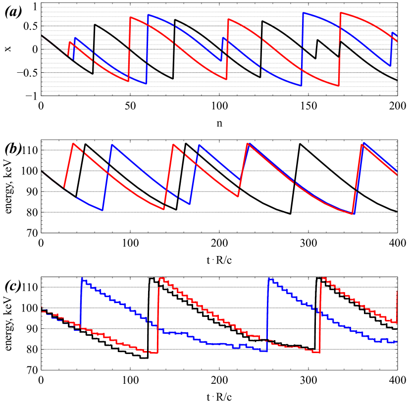
Figure 16: Panel (a) shows three trajectories $x_{n}$ for map (26) with $\Delta x_{0}=10^{-3/2}$. Panel (b) shows three trajectories $m_{e}c^{2}(\gamma_{n}-1)$ for map (25). Panel (c) shows three trajectories obtained by numerical integration of Hamiltonian equations (2). Results in panels (b,c) are obtained for initial energy $100$ keV, initial pitch-angle $\alpha_{eq}=60^{\circ}$, wave amplitude $300$ pT, and $L$-shell$=6$. Other systems parameters are the same as in Fig. 2.

For realistic systems, ${\cal S}(\gamma)$ should be derived based on actual wave field and background magnetic field latitudinal profiles. Using such realistic ${\cal S}(\gamma)$, we plot $\gamma_{n}$ trajectories in Fig. 16(b) and compare them with trajectories obtained by direct numerical integration of Hamiltonian equations (2), which are plotted in Fig. 16(c). This comparison demonstrates that the map (25) describes well the main constitutive elements of the dynamics of $\gamma$. Note that the map (25) includes a significant randomization factor (the random $\xi$) and, therefore, we cannot expect a one-to-one similarity (at each time) between the $\gamma_{n}$ profiles obtained from the map and from numerical integration of Hamiltonian equations, even if both trajectories start with the same initial conditions. However, the most important point is that the statistical properties of the $\gamma_{n}$ dynamics are the same for trajectories obtained by the mapping technique and by direct numerical integration of Hamiltonian equations.

4.6 Nonlinear resonances with multiple waves

Kinetic equations (19) and (LABEL:eq:kinetic1D_tau) have been derived for a 1D system with $h=const$, i.e., for a system including only one monochromatic wave. If we consider a more realistic situation where electrons interact resonantly with various waves having different frequencies, we cannot use this 1D approximation, because for each wave frequency we will correspond to a different $h$ given by Eq. (4). This means that the frequency value determines the shape of resonance curves in the velocity, energy space, and for different frequencies the wave-particle resonance move electrons along different curves. Moreover, $I$ also depends on wave frequency (or wave number $k$), and for each wave frequency we have a corresponding $I$, i.e., in the system with two wave frequencies we have $I_{1}$ and $I_{2}$. During the resonant interaction with the first wave, $I_{1}$ changes but $I_{2}$ is conserved, and vice versa. Therefore, for each resonance electrons move along the corresponding resonance curve. The conservation of $h$ and of one of the momenta ($I_{1}$ or $I_{2}$) leads to a one-dimensional electron dynamics in the energy/pitch-angle space, and if there is only one wave in the system electrons never leave the corresponding single resonance curve. However, electron dynamics becomes 2D in the presence of two waves, when both $I_{1}$ and $I_{2}$ change. Figure 17 illustrates this effect by showing electron resonant interactions with a single wave and with two waves. The electron moves along resonance curves and jumps between these curves due to $I_{1,2}$ jumps. Accumulation of such jumps between resonance curves ultimately leads a single electron trajectory to cover the entire energy/pitch-angle space [see more details in Artemyev, Neishtadt, Vasiliev, Zhang, Mourenas & Vainchtein, 2021].

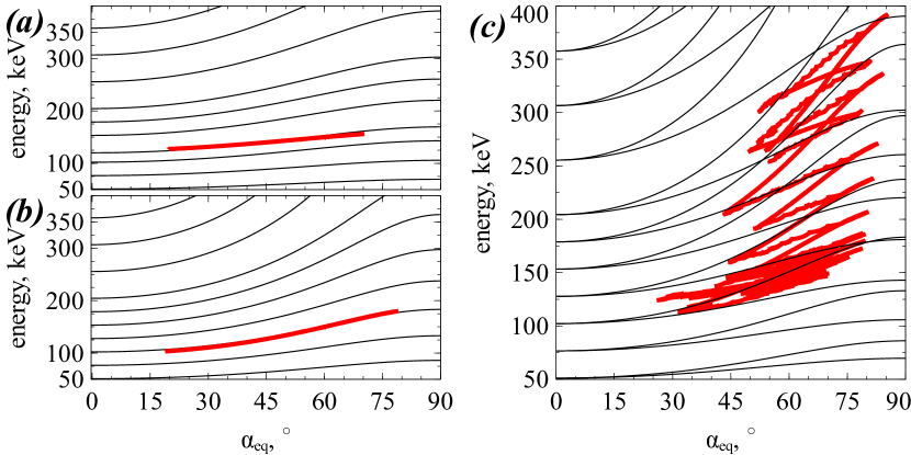
Figure 17: Top panels show resonance curves (black) and electron trajectories in the energy/pitch-angle space for Hamiltonian (2), when the electron interacts only with the first whistler-mode wave (a), only with the second whistler-mode wave (b), or with both whistler-mode waves (c). Wave frequencies are $\omega_{1}=0.4\Omega_{eq}$, $\omega_{2}=0.2\Omega_{eq}$, both wave amplitudes are $300$ pT, $L=6$, and other system parameters are from Fig. 2.

As emphasized earlier, to generalize kinetic equations (19) and (LABEL:eq:kinetic1D_tau) for systems with multiple waves, we need to use a probabilistic approach. We introduce a probability distribution function ${\cal P}(B_{w},\omega)$ that determines the wave characteristics $(\omega,B_{w})$ during the next resonant interaction. And then we average all operators in these equations over ${\cal P}$. Since such averaging significantly complicates the kinetic equations, we need an alternative approach. Let us discuss three possible methods for modeling the evolution of the electron distribution due to multiple resonances with a wave ensemble. Although we are speaking about a wave ensemble, it is assumed that electrons interact resonantly with only one monochromatic wave at a time, without the wave resonance overlap [see discussion in Tao et al., 2013; An, Wu & Tao, 2022; Gan et al., 2022], while the resonant waves may have different properties during different bounce period.

Green function approach

The Green function approach Furuya et al. [2008]; Omura et al. [2015] assumes that systems with multiple different waves (or with a single wave with evolving characteristics) can be described using Eq. (1) with a kernel derived from test-particle simulations. Figure 18(a) shows the basic scheme of this approach: test particle simulations provide the probability distribution function of energy and pitch-angle changes, and this function is used to construct the kernel and rewrite the Smoluchowski equation as

$$\begin{array}[]{l}f_{n+1}\left({E,\alpha_{eq}}\right)=\int\limits_{0}^{\infty}{dE^{\prime}\int\limits_{0}^{\pi/2}{f_{n}\left({E^{\prime},\alpha^{\prime}_{eq}}\right)G\left({\left.{E,\alpha_{eq}}\right|E^{\prime},\alpha^{\prime}_{eq}}\right)d\alpha^{\prime}_{eq}}}\\ G\left({\left.{E,\alpha_{eq}}\right|E^{\prime},\alpha^{\prime}_{eq}}\right)={\cal C}\left[{\delta\left({E-E^{\prime},\alpha_{eq}-\alpha^{\prime}_{eq}}\right)}\right]\\ \end{array}$$

where $\partial f/\partial t$ is replaced by a discrete difference $f_{n+1}-f_{n}$ during each time step of one bounce period, and $f_{n}$ is included into the Green function

$$\int\limits_{0}^{\infty}{dE^{\prime}\int\limits_{0}^{\pi/2}{G\left({\left.{E,\alpha_{eq}}\right|E^{\prime},\alpha^{\prime}_{eq}}\right)d\alpha^{\prime}_{eq}}=1}$$

while ${\cal C}$ is the particle scattering operator describing energy and pitch-angle change during a single bounce period. This operator can be obtained from test particle simulations: a large particle ensemble can be traced across the resonance and the variations of their energy and pitch-angles can be combined to determine the probabilities of all possible transports $(E^{\prime},\alpha_{eq}^{\prime})\to(E,\alpha_{eq})$ Furuya et al. [2008]. This is quite a powerful approach for quantitatively describing multiple nonlinear resonant interactions affecting the dynamics of energetic electron fluxes. Several important results have been obtained this way, like that description of the formation of relativistic/ultra-relativistic electron populations due to turning acceleration by field-aligned waves Omura et al. [2015] or due to the Landau and high-order resonances with oblique waves Hsieh & Omura [2017a]; Hsieh et al. [2020], and investigations of rapid scattering and losses of energetic electrons due to a combination of the Landau and cyclotron nonlinear resonances Hsieh et al. [2022]; Hsieh & Omura [2023]. These simulations demonstrated that the Green function approach is really promising and, combined with the observed wave distributions, it can potentially replace and supersede standard simulations of radiation belt dynamics based on the Fokker-Planck diffusion equation. The main technical difficulty of this approach is the need to predefine the resolution in energy and pitch-angle for the ${\cal C}$ operator that will be determined using test particle simulations. For instance, typical nonlinear wave-particle interactions with intense waves often cover at least three order of magnitude of energies, $[1,1000]$ keV, whereas a simultaneous inclusion of electron scattering by weak waves requires a minimum energy bin size about $10-100$eV [see typical diffusion rate magnitudes in Glauert & Horne, 2005; Horne, Kersten, Glauert, Meredith, Boscher, Sicard-Piet, Thorne & Li, 2013]. Therefore, to accurately incorporate the effects from both intense and weak waves, one would need $10^{4}-10^{5}$ energy bins and about the same number of pitch-angle bins. Thus filling the corresponding $2D$ matrix for ${\cal C}$ is computationally very expensive. Consequently, the Green function approach is useful mostly for describing electron flux dynamics in a system with intense waves (during active geomagnetic conditions), when the energy and pitch-angle bin sizes can remain sufficiently large. The two alternative methods described below, the Probabilistic approach and the Mapping technique, would require similarly huge numbers of small energy and pitch-angle bins for an accurate description of electron dynamics in the presence of both intense and weak waves, but as we will see, with potentially different intrinsic accuracy and total CPU time. The main differences of the (Probabilistic approach and Mapping technique) from the Green function approach consists in the analytical evaluation of the basic properties (characteristics) of wave-particle resonant interactions. This improves the accuracy of the evaluation of such characteristics, but reduces the flexibility for including comprehensive details of wave-particle interactions (like wave frequency drift and wave-packet structure). Roughly speaking, the Green function approach is ideal for a detailed modeling of short-term dynamics of electron fluxes, when peculiarities of wave-field can play the most important role, the Probabilistic approach is optimal for the inclusion of nonlinear resonant effects into existing numerical schemes of radiation belt dynamics (an even simpler technique for such an inclusion is discussed in Section 7), and the Mapping technique is the most suitable for observation-based modeling of meso-scale events, when wave characteristics are derived from spacecraft observations, and for incorporation of wave-particle resonant interactions into global test-particle simulations (see discussion in [Artemyev, Neishtadt & Angelopoulos, 2022] and in Section 6.3).

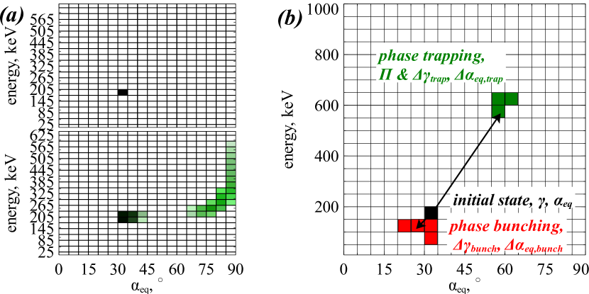
Figure 18: (a) Schematic view of the Green function approach. Numerical simulations are performed to obtain energy, pitch-angle distribution of electrons after resonant interactions (bottom panel) for electrons having the same initial energy, pitch-angle (top panel). Such distributions, obtained for different wave characteristics and for all energy, pitch-angle bins are combined into the Green function $G\left({\left.{E,\alpha_{eq}}\right|E^{\prime},\alpha^{\prime}_{eq}}\right)$ that describes the probability of $(E^{\prime},\alpha_{eq}^{\prime})\to(E,\alpha_{eq})$ transition [see details in Omura et al., 2015]. (b) Schematic view of the probabilistic approach, where for each energy, pitch-angle bin the analytical model (for a given distribution of wave characteristics) provides the probability $\Pi$ and energy, pitch-angle changes due to phase trapping (green) and due to phase bunching (red) [see details in Vainchtein et al., 2018].

Probabilistic approach

An alternative to the Green function approach and a different way of rewriting the Smoluchowski equation was proposed in Vainchtein et al. [2018]. This approach is based on the idea of separating phase trapping and bunching processes and their analytical evaluations. In this case, the discretization of the electron energy, pitch-angle space allows constructing a matrix $\hat{R}$ of energy, pitch-angle probability jumps. Within this approach, Eq. (1) takes the form

$$\frac{{\partial f_{ij}}}{{\partial t}}=-\frac{{N_{ij}}}{{\tau_{ij}}}\int\limits_{W}{{\cal P}\left(W\right)dW}+\left({\int\limits_{W}{\sum\limits_{k,l}{\hat{M}_{ij}^{kl}\left(W\right){\cal P}\left(W\right)dW}}}\right)f_{ij}$$ (27)

where $f_{i,j}=f(E_{i},\alpha_{eq,j})$, $N_{ij}=N(E_{i},\alpha_{eq,j})$ is the number of resonant interactions that particles undergo during a single bounce period $\tau_{ij}=\tau(E_{i},\alpha_{eq,j})$, $W=({\cal B}_{w},\omega)$ are wave characteristics and ${\cal P}(W)$ is the probability distribution function of wave characteristics normalized in such a way that $\int_{W}{\cal P}(W)dW$ is the ratio of the total time interval of spacecraft wave measurements to the cumulative time interval of observations of intense waves resonating with electrons nonlinearly. The operator $\hat{M}_{ij}^{kl}(W)$ is a 4D matrix describing the transformation of the 2D matrix $f_{ij}$ of initial energy, pitch-angle to a $f_{kl}$ matrix of energy, pitch-angle after one bounce period.

A schematic view of this probabilistic approach is provided in Fig. 18(b): for each energy, pitch-angle bin and each pair of wave characteristics $({\cal B}_{w},\omega)$, we determine the probabilities of particle coming and leaving due to the phase trapping and phase bunching. These probabilities are determined using the analytical model of wave-particle nonlinear interaction and, therefore, do not require large numerical test-particle simulations. Next, the matrices $\hat{R}(W)$ are averaged over the probability distributions of wave characteristics. The averaged matrix is used in the equation for the electron distribution function. The main advantage of this approach is that it is based on an analytical model of energy changes and trapping probabilities that can be rapidly evaluated over a wide parametric domain with arbitrarily high accuracy. The main disadvantage is that such analytical equations do not allow a simple generalization for more sophisticated and realistic waveforms (see discussion in Section 5). However, even such an idealized approach can still provide important information about systems with nonlinear wave-particle interactions. Specifically, numerical simulations of electron distribution dynamics with realistic and wave distributions, ${\cal P}({\cal B}_{w},\omega)$, have shown the importance of appropriately choosing the initial electron distributions Vainchtein et al. [2018]. The evolution of the electron distribution function due to nonlinear wave-particle interactions leads to a rapid change of the total electron energy, but the energy of a whistler-mode wave is not sufficient in itself to provide such an deceleration/acceleration [see discussion and estimates in Shklyar, 2011]. Therefore, the large population of scattered (decelerated) electrons provides the only available energy source for trapped electron acceleration. The corresponding energy balance imposes several constraints on the initial electron distribution function for models describing nonlinear interactions. This initial distribution should be consistent with the conservation of the total energy for solutions of Eq. (27). Vainchtein et al. [2018] checked the total particle energy variation for different initial pitch-angle distributions: an initial distribution with transverse anisotropy ($F\propto\sin\alpha_{eq}$) immediately loses energy, whereas a field-aligned anisotropic distribution ($f\propto\cos\alpha_{eq}$) first gains energy before losing it. More specific distributions (butterfly $f\propto\sin 2\alpha_{eq}$ sometimes observed in the radiation belts [see statistics in Åsnes et al., 2005] and a distribution with field-aligned beams $f\propto\sin\alpha_{eq}\cos^{4}\alpha_{eq}$ observed during particle injections [e.g., Mozer et al., 2016]) show energy increase during the first stage of the evolution. This suggests that for a $f$ to result in total energy conservation it should be more isotropic (i.e., an intermediate state between transverse anisotropy $\sim\sin\alpha_{eq}$ and field-aligned anisotropy $\sim\cos\alpha_{eq}$). Moreover, under realistic conditions, particle anisotropy is energy dependent, and can be different for $<100$ keV particles and $\sim 1$ MeV particles. Therefore, further investigations of particle distributions consistent with the assumption of total energy conservation are needed to accurately model nonlinear wave-particle interactions [see, also, Shklyar, 2017; Shklyar & Luzhkovskiy, 2023, for details on the relation between trapped and scattered electron populations in a system with small variations of wave intensity].

Mapping technique

The mapping technique can easily be generalized to multi-wave systems: instead of Eq. (25) for a single wave, we should use

$$\gamma_{n+1}=\gamma_{n}+\left\{{\begin{array}[]{*{20}c}{\Delta\gamma_{trap}\left({\eta_{n},\gamma_{n}}\right),}&{\xi_{n}\in\left[{0,\Pi\left({\eta_{n},\gamma_{n}}\right)}\right)}\\ {\Delta\gamma_{bunch}\left({\eta_{n},\gamma_{n}}\right),}&{\xi_{n}\in\left({\Pi\left({\eta_{n},\gamma_{n}}\right),1}\right]}\\ \end{array}}\right.$$ (28)

where the index $\eta_{n}$ is a random number with a probability distribution such that $\eta$ determines the probability of resonant interaction with different waves, which characteristics are given by the distribution ${\cal P}(B_{w},\omega)$. Thus, before each resonant interaction (each $\gamma$ change) with a particular particle, we determine from ${\cal P}(B_{w},\omega)$ the corresponding wave, and use the corresponding ${\cal S}$ to determine energy, pitch-angle change for this particle. Particle pitch-angles should be recalculated with new $\gamma_{n+1}$ and corresponding wave frequency $\omega$ accordingly to Eq. (4). Figure 19(a) shows several examples of electron trajectories evaluated with the mapping (28) for the wave probability distribution ${\cal P}(B_{w},\omega)$ from panel (c). This distribution contains waves of different frequencies, and for each frequency the resonant interaction will move electrons along the $h(\omega)=const$ curve (see Eq. (4)). Phase bunching moves electrons along $h=const$ curves with energy and pitch-angle decrease (see the prolonged intervals with energy decrease in panel (a)), whereas phase trapping moves electrons along the same curves, but with an energy increase (see the rare positive energy jumps in panel (b)). For a single frequency system, there would be only one curve $h=const$ for each initial electron energy, pitch-angle, and thus electrons would move along this curve in the energy, pitch-angle space. But the system in Fig. 19 contains multiple frequencies and, thus, resonant interactions will provide complex electron dynamics in the 2D energy, pitch-angle space. Figure 19(b) shows two trajectories from panel (a) in the energy, pitch-angle space: drifting from one resonant curve to another one, electrons may increase their energy with a net pitch-angle decrease (see also Fig. 17(c)), which is purely due to resonant interactions with different waves at multiple frequencies. Note that the distribution shown in Fig. 19(c) contains many waves with an amplitude insufficiently large to resonate with a particular electron nonlinearly. Such waves should provide electron diffusive scattering, which is not included into the mapping given by Eq. (28). Such diffusive scattering can be incorporated into the mapping scheme using standard (Chirikov-type, see Chirikov [1987]) maps. Examples of such maps can be found in Vasilev et al. [1988]; Zaslavskii et al. [1989]; Khazanov et al. [2013, 2014].

The map (28) can be used with a 3D wave characteristic distribution ${\cal P}={\cal P}(B_{w},\omega,\theta)$, but then, we need to use a different Eq. (4) for a different resonance number. Generally two main resonances, Landau resonance with very oblique waves (${n_{r}}=0$) and the first cyclotron resonance with quasi-parallel waves (${n_{r}}=1$), are included Artemyev, Neishtadt, Vasiliev, Zhang, Mourenas & Vainchtein [2021]. The difference is in relation of $I$ from Eq. (4) and the electron magnetic moment $I_{x}$: for ${n_{r}}=0$ Eq. (4) becomes $I_{x}=const$, whereas for ${n_{r}}=1$ Eq. (4) becomes $m_{e}c^{2}\gamma-\omega I_{x}=const$.

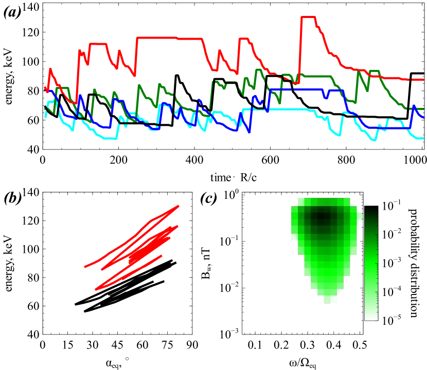
Figure 19: Panel (a) shows five examples of electron trajectories (energy vs. time) for cyclotron resonance with waves having the distribution shown in panel (c). All electrons have the same initial energy and pitch-angle. Panel (b) shows two trajectories from panel (a) in the (energy, pitch-angle) space. Background magnetic field and plasma density characteristics are the same as in Fig. 2.

Using a similar approach with a probability distribution for the waves, we may generalize the map (28) for a system with both types of whistler-mode waves: quasi-parallel and very oblique. In this case, before each resonant interaction, we determine the wave type, which in turn determines the type of resonance – Landau or cyclotron. Figure 20(a) shows examples of electron trajectories in the case where the probability for electrons to meet very oblique and quasi-parallel waves is the same. Electron energy dynamics resembles results obtained for a system including only cyclotron resonance (see Fig.19(a)): prolonged periods of energy decrease due to the phase bunching (due to both Landau and cyclotron resonances) are intermittently interrupted by rare positive jumps of energy due to phase trapping (related to both Landau and cyclotron resonances). The main difference with the cyclotron-resonance-only system (including only parallel waves) from Fig. 19 is that energy increases/decreases in Landau resonance correspond to pitch-angle decreases/increases, such that Landau phase trapping, in particular, results in simultaneous acceleration and pitch-angle decrease. Together, nonlinear wave-particle interactions through cyclotron and Landau resonances with parallel and oblique waves provide both significant electron acceleration and efficient transport toward the loss-cone (see Fig.20(b) and compare with Fig.19(b)) and, therefore, lead to an enhanced precipitation of energetic (accelerated) electrons compared with a system including only cyclotron resonance with parallel waves [see more details of this effect in Mourenas et al., 2016; Hsieh et al., 2022].

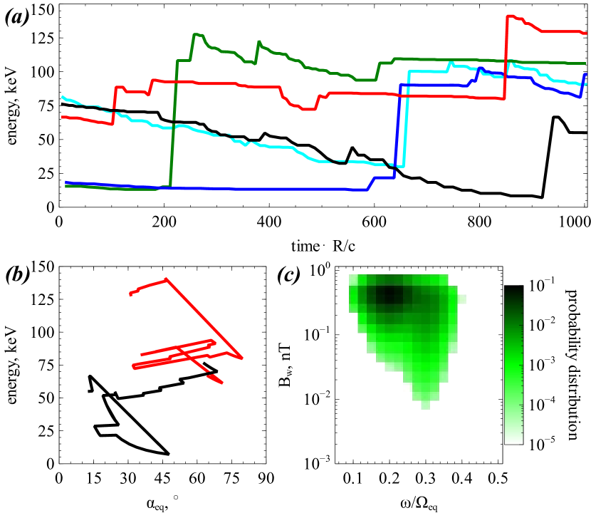
Figure 20: Panel (a) shows five examples of electron trajectories (energy vs. time) for Landau and cyclotron resonances with waves having the distribution shown in panel (c). All electrons have the same initial energy and pitch-angle. Panel (b) shows two trajectories from panel (a) in the (energy, pitch-angle) space. Background magnetic field and plasma density characteristics are the same as in Fig. 2.

Such mapping simulations of individual electron trajectories (energy as a function of the resonant interaction number or time) can be combined to comprehensively describe the full dynamics of the electron distribution function [Artemyev, Neishtadt, Vasiliev, Zhang, Mourenas & Vainchtein, 2021; Artemyev, Zhang, Zou, Mourenas, Angelopoulos, Vainchtein, Tsai & Wilkins, 2022; Zhang, Artemyev, Angelopoulos, Tsai, Wilkins, Kasahara, Mourenas, Yokota, Keika, Hori, Miyoshi, Shinohara & Matsuoka, 2022]. Therefore, the mapping technique may provide the same level of system description as the probabilistic approach and Green function approach.

5 Effects of short wave-packets

The general theoretical results described by Eqs. (19) and (28) were obtained in the simplified case of a plane wave (such that the term $\sim B_{w}$ contains only $\sin\zeta$ in Hamiltonian (2)). However, in realistic plasma systems, such very long wave-packets (such that the wave packet envelope can be neglected) are rarely observed, and most of the whistler-mode waves present in the outer radiation belt are propagating in the form of short wave-packets (see examples in Fig. 21(a,b) and [Zhang, Thorne, Artemyev, Mourenas, Angelopoulos, Bortnik, Kletzing, Kurth & Hospodarsky, 2018; Zhang, Mourenas, Artemyev, Angelopoulos, Bortnik, Thorne, Kurth, Kletzing & Hospodarsky, 2019]). Typical wave-packets (or subpackets) comprise several (up to ten) wave periods and reach moderate peak amplitudes (${\cal B}_{w}\approx 100-300$ pT), but the most intense (${\cal B}_{w}>500$ T) wave-packets can be quite long and may include more than hundred wave periods. The formation of such long wave-packets is associated with the classical nonlinear mechanism of whistler-mode chorus wave generation [see reviews in Demekhov, Taubenschuss & Santolík, 2017; Omura et al., 2013; Omura, 2021; Tao et al., 2020, 2021], and it is also the case for moderately long but intense subpackets Chen et al. [2024]. On the other hand, most of the moderate intensity short wave-packets are likely generated due to wave superposition, also called wave beating [see details in Zhang, Mourenas, Artemyev, Angelopoulos, Kurth, Kletzing & Hospodarsky, 2020; Nunn et al., 2021; Mourenas et al., 2022; An, Wu & Tao, 2022]. Detailed comparison of wave generation models and spacecraft statistics of whistler-mode wave-packets confirms this scenario of separation of short and long wave-packets Zhang et al. [2021]. Note that basic empirical models of whistler-mode waves do not include information about wave-packets Meredith et al. [2012]; Agapitov et al. [2013], and this significantly complicates the investigation of nonlinear resonant effects [see discussion in Allanson et al., 2024]. In this review, we utilize wave-packet statistics published in Zhang, Mourenas, Artemyev, Angelopoulos, Bortnik, Thorne, Kurth, Kletzing & Hospodarsky [2019]; Zhang, Mourenas, Artemyev, Angelopoulos, Kurth, Kletzing & Hospodarsky [2020].

To model this effect for a monochromatic wave, we may adopt the scheme proposed in Matsoukis et al. [2000]; Wykes et al. [2001] and rewrite the field term in Eq. (2) as

$${\cal B}_{w}(\lambda)\sin\zeta\to{\cal B}_{w}(\lambda)\exp\left(-{\cal A}\sin^{2}\left(\phi/2\ell\right)\right)\sin\zeta$$

where parameter ${\cal A}$ determines the depth of wave field modulation, $\ell$ is the wave-packet size in wave length (wave periods) units. Figure 21(c) shows examples of this wave-packet model.

An alternative and more sophisticated wave-packet model for whistler-mode chorus waves (with frequency drift) has been proposed in Furuya et al. [2008] and actively used for investigation of the effect of wave field modulation on efficiency of electron resonant dynamics [Tao, Bortnik, Thorne, Albert & Li, 2012; Tao et al., 2013; Gan et al., 2020]. This model includes the difference between group and phase wave velocities, and thus describes wave-packet modification during the propagation, because different waves contributing to each wave-packet propagate with different velocities. Kubota & Omura [2018]; Hiraga & Omura [2020]; Hsieh et al. [2020] have investigated in detail this chorus wave-packet model and incorporated it into a general scheme of electron flux evaluation in systems with multiple nonlinear resonances based on the Green function approach Omura et al. [2015].

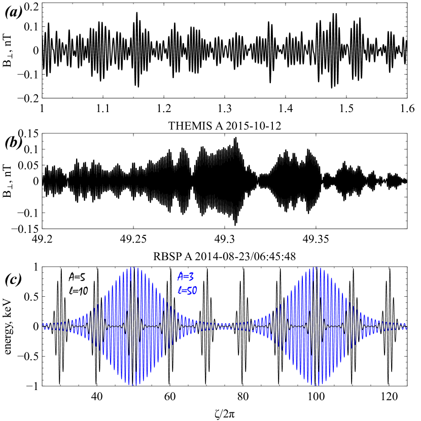
Figure 21: Panel (a,b) shows four examples of whistler-mode wave-packets propagating with a small wave normal angle: measurements from THEMIS Le Contel et al. [2008] and Van Allen Probes Kletzing et al. [2013] search-coil magnetometers ($L$-shell and $MLT$ are indicated within panels).Panel (c) shows two examples of model wave-packets.

Resonant interactions with such short wave-packets differ from the simplified picture of interaction with infinitely long packets in four main aspects:

Nonlinear phase bunching

is affected mostly by the wave-packet propagation in latitude. For an infinite wave-packet, the wave amplitude at the latitude of resonance (for fixed energy and pitch-angle) is determined by a fixed $B_{w}(\lambda)$ profile that does not depend on time. But for short wave-packets, the wave amplitude depends on the time delay between the particle and the wave-packet arriving at the latitude of resonance with that particle (see scheme in Fig. 22(a)). This significantly randomizes the effect of phase bunching and gives a broader energy distribution in comparison with results for the infinite plane wave. Figure 22(b) shows the probability distribution of energy changes due to a single resonant interaction with a very long wave-packet ($\ell=300$, $\ell=500$) and short wave-packets ($\ell=10$). In these simulations, the upper limit of the negative energy jump (the phase bunching effect) is the same, because it is determined by the peak wave amplitude, which is the same in all cases. However, for short wave-packets there is a broader distribution of negative energy changes, because particles can encounter various (randomized) instantaneous wave amplitudes at the resonance. These simulations have been set up in such a way that initial electron coordinates are uniformly distributed within the range corresponding to electrons arriving to the resonance when the wave-packet amplitude there exceeds $1/100$ of the peak value, i.e., we excluded from the simulations the particles arriving into the resonance between two successive wave-packets and which would not significantly interact with the waves.

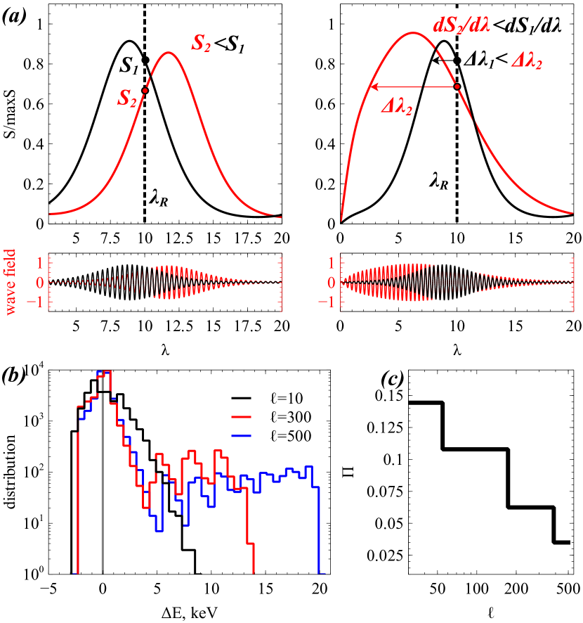
Figure 22: Panel (a) shows a schematic view of electron resonant interactions with short wave-packets. The three main parameters are the dependencies of (1) the instantaneous wave amplitude (determining the efficiency of phase bunching) at the resonance and (2) the wave amplitude gradient (determining the phase trapping probability) on the initial electron location relative to the wave-packet generated at the equator, and (3) the wave-packet size (which determines the energy gain due to phase trapping, instead of the background magnetic field gradient in the case of a very long packet). Panel (b) shows the distribution of energy changes due to a single resonant interaction with long ($\ell=300$ and $\ell=500$) and short ($\ell=10$) wave-packets. Panel (c) shows the distribution of the trapping probability, $\Pi$, for a single resonant interaction, as a function of wave-packet length, $\ell$. For numerical simulations shown in panels (b,c) we use field-aligned whistler-mode waves with a peak amplitude of $500$ pT and electrons with an initial energy of $100$ keV and an equatorial pitch-angle of $30^{\circ}$; other system characteristics are the same as in Fig. 2.

The probability of nonlinear phase trapping

is also mostly affected by the strong wave field gradient at the wave-packet edges. For an infinite wave-packet, the trapping probability is determined by the latitudinal gradients of the wave field and background magnetic field, but for short wave-packets this probability is instead determined by the gradient of the wave-packet envelope Bortnik et al. [2008]. In contrast to background latitudinal gradients, with typical spatial scales of $\sim LR_{E}\sim 10^{4}$km, the typical scale of the wave envelope gradient can shrink to only a few wavelengths, $\sim 10-100$km, which represents a huge increase of $d{\cal S}/d\gamma\propto d{\cal B}_{w}/d\lambda$ along the resonant trajectory. Figure 22(c) shows how the trapping probability depends on wave-packet size for a given wave-packet model, and increases for shorter packets. In particular, for a short wave-packet, electrons interacting resonantly with the packet leading edge have a larger probability of phase trapping.

Energy changes due to nonlinear phase trapping

are also strongly affected by the wave-packet size. For such short wave-packets, in principle phase trapping becomes possible at any latitude of resonance, without a strong influence of the background profiles of wave and magnetic fields. However, the resulting strong increase of the probability of trapping is compensated by the brevity of this trapping, because particles rapidly escape from the resonance (and from the trapping) at the edges of wave-packets. For the first cyclotron resonance, the resonant electrons and waves are propagating in opposite directions, corresponding to a maximum possible trapping time $\Delta t_{trap}\approx 2\pi\ell/k|v_{g}+v_{R}|$, where $v_{g}=\partial\omega/\partial k_{\parallel}$ denotes the wave group velocity and $v_{R}=(\omega-\Omega_{0}/\gamma)/k_{\parallel}<0$ the velocity of the particle in cyclotron resonance with the wave. Using a simple approximation $v_{g}\approx\omega/k_{\parallel}$ [for parallel propagating waves, the typical ratio of $k_{\parallel}v_{g}/\omega$ is $1-2$, see Stix, 1962], we obtain $\Delta t_{trap}\approx 2\pi\ell/\Omega_{ce}$. Thus, a finite wave-packet size directly sets an upper limit on the electron acceleration. A possible exception has been considered in Hiraga & Omura [2020], where the idea of successive trapping into series of wave-packets (wave-packet train) has been proposed. Such a mechanism allows to neglect the effect of particle detrapping at the edges of wave-packets, because such detrapped particles will soon be trapped again by the next packet. However, successive trapping requires that the wave phase remain coherent across the entire wave-packet train, without strong phase stochastization at the wave-packet edges, which limits its applicability [see examples of observations of both coherent and non-coherent wave packet trains in Zhang, Agapitov, Artemyev, Mourenas, Angelopoulos, Kurth, Bonnell & Hospodarsky, 2020].

In Figure 22(b), wave-packets are assumed to be isolated, or separated by random jumps of wave frequency and phase as in most observations [Zhang, Mourenas, Artemyev, Angelopoulos, Kurth, Kletzing & Hospodarsky, 2020; Zhang, Agapitov, Artemyev, Mourenas, Angelopoulos, Kurth, Bonnell & Hospodarsky, 2020]. Compared with long packets, short wave-packets lead to a significantly broader distribution of small positive energy changes at $\Delta E=0-5$ keV through phase trapping, due to a randomization of the duration of trapping and of the related energy change, while the maximum energy changes are strongly reduced (from 20 keV to 8 keV). Together with the randomization of phase bunching effects for negative energy changes, short wave-packets therefore lead to a more symmetrical distribution of energy changes compared with long packets.

The periodical structures present in the distribution of energy changes due to trapping for long packets ($\ell=300$ and $\ell=500$) is due to the discretization of the trapping time: trapped particles can spend in acceleration regime time intervals divisible to trapping periods $\sim 2\pi/\Omega_{tr}$. As a result, resonant particles may makes $\sim{\cal N}_{trap}$ times rotations during their trapping, with ${\cal N}_{trap}=\Delta t_{trap}\Omega_{tr}/2\pi$. Changes of this number by $\pm 1$ due to uncertainties of trapping/de-trapping time result in the formation of several peaks in the $\Delta E$ distribution [see details in Vainchtein et al., 2017].

Nonlinear anomalous phase trapping effects

are also affected, because a very long packet corresponds to one long phase trapping interval, whereas short wave-packets result in multiple trapping occurrences, more probable but much more short-lived. For medium to high pitch-angles, this leads to a modification of the probability distribution of energy changes (see an example in Fig. 22(b)), whereas for small pitch-angles this may prevent an effective particle transport away from the loss-cone, i.e., it can reduce the efficiency of anomalous trapping [see Appendix in Mourenas et al., 2022]. Figure 23 illustrates this idea: for long wave-packets a significant fraction of low pitch-angle particles are transported by anomalous trapping to higher pitch-angles [see also Kitahara & Katoh, 2019], whereas for short wave-packets the resonant interactions become less regular and anomalous trapping competes with phase bunching, leading to a global transport of initially low equatorial pitch-angle electrons to both smaller and higher pitch-angles, in roughly similar quantities (note that only the first cyclotron resonance is considered here), corresponding to a symmetrization of pitch-angle changes.

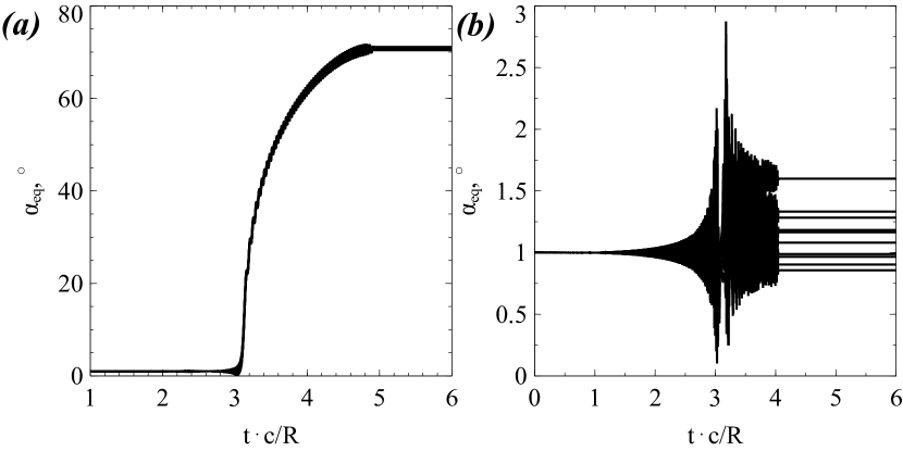
Figure 23: Dynamics of electron equatorial pitch-angles due to a single resonant interaction with a plane wave, corresponding to an infinitely long ($\ell\to\infty$) wave-packet (a) and with a short ($\ell=10$) wave-packet (b). The system parameters are the same as in Fig. 22.

5.1 Kinetic equation

Let us consider the kinetic equation (19) under the short wave-packet approximation. The effects of phase trapping at arbitrary latitude (arbitrary $\gamma$ or $I$) and the variability of the phase bunching amplitudes cannot be straightforwardly included into this kinetic equation (we shall describe these effects using the mapping technique in Sect. 6.1). Thus, we limit our consideration to the effects in a small energy (or $I$) range with $V(\gamma)\propto{\cal S}(\gamma)\neq 0$. The maximum energy change due to trapping is equal to $mc^{2}(\gamma_{\max}-\gamma_{\min})$, where $\gamma_{\min,\max}$ are boundary values of the ${\cal S}(\gamma)$ profile, i.e., ${\cal S}(\gamma_{\min,\max})=0$. Therefore, for a small range $[\gamma_{\min},\gamma_{\max}]$ we can expand the nonlocal term of Eq. (19) as:

$$f\left(\gamma^{\prime}\right)\approx f\left(\gamma\right)-\frac{{\partial f}}{{\partial\gamma}}\cdot\left({\gamma-\gamma^{\prime}}\right)\approx f-2\frac{{\partial f}}{{\partial\gamma}}\left({\gamma-\gamma_{0}}\right)$$

where $\gamma_{0}$ is the energy where ${\cal S}(\gamma)$ reaches its peak value. Substituting this expansion into Eq. (19), we obtain

$$\frac{{\partial f}}{{\partial t}}=\frac{\partial}{{\partial\gamma}}\left({D_{\gamma\gamma}\frac{{\partial f}}{{\partial\gamma}}}\right)-\tilde{V}\frac{{\partial f}}{{\partial\gamma}},\quad\tilde{V}=V_{\gamma}+2\frac{{dV_{\gamma}}}{{d\gamma}}\left({\gamma-\gamma_{0}}\right)\Theta$$

(29)

$$\Theta=1,\quad\gamma>\gamma_{0},\quad\&\quad\Theta=0,\quad\gamma<\gamma_{0}$$

Using the variable $x=(\gamma-\gamma_{0})/\left(\gamma_{\max}-\gamma_{\min}\right)$ with $\gamma_{0}=\left(\gamma_{\max}+\gamma_{\min}\right)/2$ and ${\cal S}$ from Eq. (21), we can write

$$V_{\gamma}=-V_{0}\left({1-x^{2}}\right)^{5/4},\quad\tilde{V}=-V_{0}\left({1-x^{2}}\right)^{1/4}\left({1-x^{2}\left({5\Theta+1}\right)}\right)$$

Figure 24(a) shows the profile of $\tilde{V}(x)$: $\tilde{V}$ is positive for $x<0$ ($\gamma<\gamma_{0}$, $\Theta=0$) and negative for $x>1/\sqrt{6}$ ($\gamma>0$, $\Theta=1$). Therefore, electrons with $x>1/\sqrt{6}$ and $x<1/\sqrt{6}$ are drifting in opposite directions, corresponding to the opposite effects of trapping-induced acceleration and deceleration by nonlinear scattering.

If we omit the diffusion term, $\sim D_{\gamma\gamma}$, Eq. (29) represents a simple drift equation

$$\frac{{\partial f}}{{\partial t}}=-\tilde{V}\left(x\right)\frac{{\partial f}}{{\partial x}},$$

and for an initial condition $f_{t=0}(x)$ this equation has an analytical solution: $f$ is a constant along trajectories $t-\int{dx/\tilde{V}(x)}=const$. The function $\int{dx/\tilde{V}(x)}\to\pm\infty$ at $x=1/\sqrt{6}$ where $\tilde{V}(x)=0$, implying that the particles should drift in energy space away from $x=1/\sqrt{6}$. Indeed, the solution of the drift equation displayed in Figure 23(b) demonstrates the formation of a plateau in energy space around $x=1/\sqrt{6}$. This effect is essentially the same as what occurs during the well-known quasi-linear evolution of a particle distribution function: resonant wave-particle interactions result in a flattening of the phase space density profile within the range of resonant energies [e.g., Galeev & Sagdeev, 1979; Vedenov & Ryutov, 1975]. However, in contrast with quasi-linear diffusion, this peculiar type of nonlinear interaction is much faster and corresponds to drifts $\sim\tilde{V}\propto\left({\cal B}_{w}/B_{0}\right)^{1/2}$. Figures 23(c,d) confirm this theoretical result of plateau formation within a narrow energy range for particles interacting resonantly with short wave-packets. These figures show the results of a numerical integration of Hamiltonian equations of motion for a large particle ensemble interacting with a monochromatic wave-packet (so that Eq. (4) is well satisfied and we may consider a 1D evolution of the particle distribution function).

Note that the location $x=1/\sqrt{6}$ of the plateau formation shown in Figure 23(b) is largely determined by the system parameters, while for an ensemble of wave-packets (even if such packets are well separated in space and time) these plateaus will be formed around different $x$ (at different energies). Therefore, the global evolution of the electron distribution function can ultimately lead to a reduction of phase space density gradients over a wide energy range [see Section 6 and Artemyev, Neishtadt, Vasiliev & Mourenas, 2021, for details of such evolution].

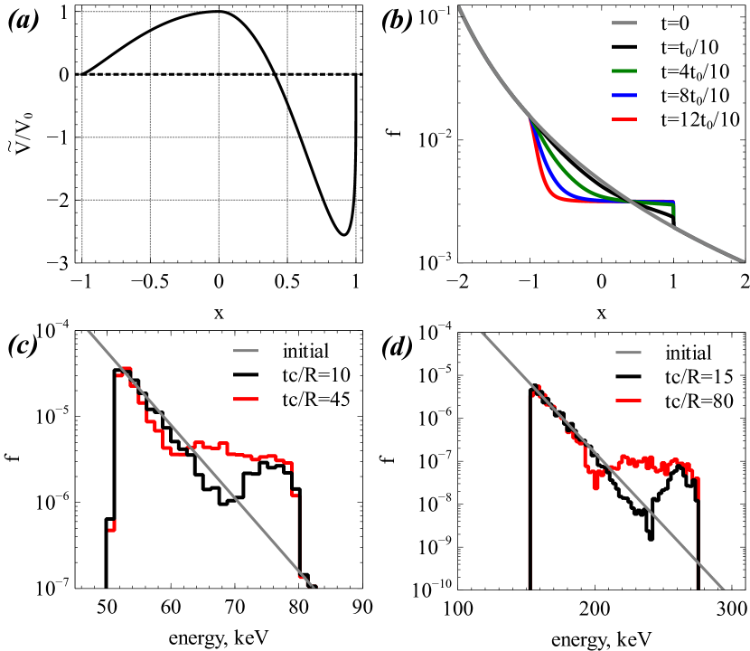
Figure 24: Panel (a) shows the profile of $\tilde{V}(x)/V_{0}$. Panel (b) shows the solution to Eq. (29) at several times $t$, with $t_{0}=V_{0}\cdot R/c$. Panels (c, d) show two examples of numerical solutions, using test particle tracing. System parameters are the same as in Fig. 2, but we use a wave amplitude ${\cal B}_{w}=100$ pT and a wave packet size $\ell=15$. Two values of the constant $h$ from Eq. (4) are used: $h=1.1$ (c) and $h=1.3$ (d).

5.2 Limit of nonlinear diffusion

Shorter wave-packets correspond to smaller energy changes due to trapping and a higher trapping probability (due to the high probability for electrons to resonate with wave-packet edges having a strong $d{\cal S}/d\gamma\propto dB_{w}/d\lambda$ gradient). Therefore, as discussed earlier, the decrease of the wave-packet size should lead to a more symmetrical $\Delta E$ distribution (e.g., see Figs. 22(b) and 25, and the works from Tao et al. [2013]; Zhang, Agapitov, Artemyev, Mourenas, Angelopoulos, Kurth, Bonnell & Hospodarsky [2020]; An, Wu & Tao [2022]; Gan et al. [2022]; Frantsuzov et al. [2023]). The natural limit is the fully symmetrical $\Delta E$ distribution with $\langle\Delta E\rangle\sim 0$ and an equal amount of trapped and phase bunched particles. This regime of wave-particle resonant interactions is equivalent to diffusion, but the diffusion rate may not anymore linearly depend on wave intensity, contrary to the case of quasi-linear diffusion, where we have $\langle(\Delta E)^{2}\rangle\propto{\cal B}_{w}^{2}$ Kennel & Engelmann [1966]. Let us examine this regime of nonlinear diffusion in more detail. We start with test particle simulations showing the $\Delta E$ distributions for different wave amplitudes $B_{w}$ and wave-packet sizes. Figure 25 shows $\Delta E$ distributions obtained from a numerical integration of Hamiltonian equations (2) with

$$B_{w}=B_{w,peak}\frac{{1-\exp\left({-{\cal A}\sin^{2}\left({\phi/2\ell}\right)}\right)}}{{1-\exp\left({-{\cal A}}\right)}}$$

where $B_{w,peak}$ is the peak wave amplitude, $\ell$ defines the number of wave oscillations (periods) within one wave packet, and ${\cal A}$ controls the depth of amplitude modulations. We also introduce the effective wave amplitude, which corresponds to the wave intensity averaged over the wave-packet size:

$${\cal B}_{w}=\sqrt{\left\langle B_{w}^{2}\right\rangle}_{\phi\in[0,2\pi l]}=B_{m}\frac{\sqrt{1-2I_{0}\left({\cal A}/2\right)e^{-{\cal A}/2}+I_{0}\left(h\right)e^{-{\cal A}}}}{1-e^{-{\cal A}}}$$

where $I_{n}(z)$ is the modified Bessel function of the first kind.

Figure 25(a) shows the detailed distribution of individual (separate) electron energy changes $\Delta E$ for long wave packets. For small wave amplitudes, ${\cal B}_{w}/B_{0}<5\cdot 10^{-4}$, the distribution is symmetric relative to $\Delta E=0$ with a dispersion scaling as $\langle(\Delta E)^{2}\rangle\propto({\cal B}_{w}/B_{0})^{2}$. This is the regime of purely diffusive electron scattering. As the wave amplitude increases, the $\Delta E$ distribution shows the formation of a population of phase trapped particles with $\Delta E\sim 10$ keV (well separated from the main distribution) and of a large population of phase bunched particles (increase of the probability for $\Delta E<0$ in comparison with the probability of $\Delta E>0$; the distribution boundary scales with wave amplitude as $\propto\sqrt{{\cal B}_{w}/B_{0}})$. This is the standard picture of nonlinear resonant interactions with plane waves or very long wave-packets, when two distinct populations of phase trapped and phase bunched particles are formed, well separated in the $\Delta E$ space.

Figure 25(b) demonstrates the effect of including a wave-packet modulation, corresponding to electron interaction with a short wave-packet. The main difference with Fig. 25(a) is the absence of a distinct asymmetry in the $\Delta E$ distribution for large wave amplitudes, ${\cal B}_{w}/B_{0}<5\cdot 10^{-4}$. Although some asymmetry of $\Delta E>0$ vs. $\Delta E<0$ is present, the $\Delta E$ distribution is much more symmetric when a short wave-packet modulation is included, with a larger population of $\Delta E>0$. Such symmetrization occurs because the wave amplitude modulation, or limited size, of a short wave-packet, leads to a randomization of the magnitudes and occurrences of nonlinear effects, such that phase trapping provides smaller and more random, but also more probable energy increases, while phase bunching provides more random energy decreases [see also Tao et al., 2013; Zhang, Agapitov, Artemyev, Mourenas, Angelopoulos, Kurth, Bonnell & Hospodarsky, 2020; An, Wu & Tao, 2022]. As a result, the main effect of a wave-packet modulation (i.e., of a limited wave-packet size) is a symmetrization of the $\Delta E$ distribution, such that wave-particle interactions become more diffusive-live, even in the limit of high wave amplitudes. Note that the dispersion of the $\Delta E$ distribution for large amplitudes scales with ${\cal B}_{w}$ as $\langle(\Delta E)^{2}\rangle^{1/2}\propto\sqrt{{\cal B}_{w}/B_{0}}$, i.e., the diffusion by intense modulated wave-packets does differ from quasi-linear diffusion.

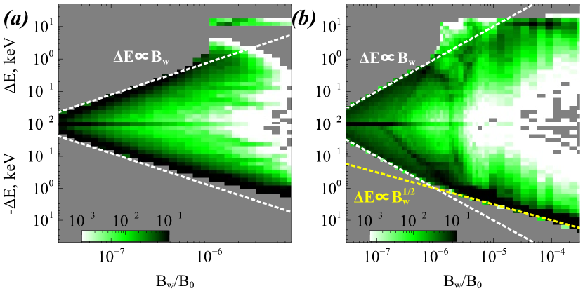
Figure 25: Distributions of energy changes $\Delta E$ for different $B_{eff}/B_{0}$ with ${\cal A}=0$ (a) and ${\cal A}=1$ and $\ell=20$ (b) waves, with $\Delta E\propto B_{w}$ fits (white dashed lines). System parameters are $E_{0}=100$ keV, $\alpha_{eq}=60^{\circ}$, $L\text{-shell}=6$, whistler-mode waves with a frequency equal to $0.35$ of the electron cyclotron frequency at the equator, and a constant plasma frequency equal to $10$ of the electron cyclotron frequency at the equator. For each $B_{eff}$, we use $10^{4}$ trajectories to evaluate the $\Delta E$ distribution, each particle resonating with the wave only once, and $\Delta E$ being the energy change for a single resonance. Initial particle and wave phases are random and thus in the modulated amplitude case the actual wave amplitude is different for different particles having the same energy/pitch-angle. See details in Frantsuzov et al. [2023].

Let us briefly consider the limit of extremely short wave-packets, corresponding to fully incoherent waves. In such a case, the $\Delta E$ distribution can be characterized by its variance alone, and the only system characteristic is the diffusion coefficient. Note that this is only an ideal limiting case: it should not be confused with the case of usual short wave-packets that lead to both energy diffusion and distinct energy drifts due to phase trapping and bunching. This ideal limiting case is interesting, though, because we can derive the corresponding characteristic diffusion coefficient analytically, using Eq. (3), as the resonant scattering is then a purely local process (in contrast with phase trapping that depends on the wave-packet shape determining the ${\cal S}(\gamma)\neq 0$ energy range). For such local processes, the wave-packet shape can be simply taken into account by introducing an effective wave amplitude parameter ${\cal B}_{w}$. Equation $m_{e}c^{2}\Delta\gamma=\omega\Delta I$ and (3) provide the energy change due to a single resonant interaction for an arbitrary wave intensity (exceeding the quasi-linear threshold) and, therefore, can be used to evaluate the variance of energy changes:

$$\left({\Delta\gamma}\right)^{2}=\left({\frac{{\omega\sqrt{2M\left|{\rm A}\right|}}}{{m_{e}c^{2}}}}\right)^{2}F^{2}\left({\xi,a}\right)$$

Figure 9(b) shows $\left\langle{F^{2}}\right\rangle_{\xi}$ and its mean value, $\left\langle{F}\right\rangle_{\xi}$, evaluated as a function of parameter $a\propto{\cal B}_{w}$. The variance has a peak at $a=1$, the boundary value between the weak wave approximation (no phase trapping and bunching for $a<1$) and the intense wave approximation ($a>1$). The diffusion coefficient for such intense waves takes the form

$$\left\langle{\left({\Delta\gamma}\right)^{2}}\right\rangle_{\xi}=\left({\frac{{\omega\sqrt{2M\left|{\rm A}\right|}}}{{m_{e}c^{2}}}}\right)^{2}\left\langle{F^{2}\left({\xi,a}\right)}\right\rangle_{\xi}$$ (30)

and for very large wave amplitudes, $a\gg 1$, this coefficient has an asymptotic form Frantsuzov et al. [2023]

$$\left\langle{\left({\Delta\gamma}\right)^{2}}\right\rangle_{\xi}\approx\left({\frac{{\omega\sqrt{2M\left|{\rm A}\right|}}}{{m_{e}c^{2}}}}\right)^{2}\frac{{32a}}{{\pi^{2}}}=\frac{{64}}{{\pi^{2}}}\left({\frac{\omega}{{m_{e}c^{2}}}}\right)^{2}M{\rm B}\propto{\cal B}_{w}$$

Therefore, the diffusion rate corresponding to intense monochromatic waves in the ideal limit of extremely short packets increases with wave intensity weaker than expected based on quasi-linear theory, where $D\propto{\cal B}_{w}^{2}$. Figure 26 illustrates this effect: the diffusion rate scales with ${\cal B}_{w}$ as $D\propto{\cal B}_{w}^{2}$ up to the threshold for nonlinear resonant interactions, ${\cal B}_{w}^{*}$, and then significantly decreases relative the $D\propto{\cal B}_{w}^{2}$ expectation. This effect has been noted in numerical verifications of the quasi-linear diffusion equations, which demonstrated that the diffusion rate is lower than the expected quasi-linear level for fully incoherent waves of high intensity Tao, Bortnik, Albert & Thorne [2012]; Gan et al. [2022]. These results underline that even extremely short, strongly modulated wave-packets will not lead to a purely quasi-linear diffusion of electrons for a sufficiently high wave intensity: in such a case, the wave intensity cannot be used anymore as a simple scaling factor [i.e., the procedure of wave intensity averaging over spatial and temporal domains may affect the estimation of the diffusion rate; see also Watt et al., 2017, 2021, for discussion of a similar effect of temporal/spatial variability of diffusion rates].

A natural question arising from the results in Fig. 26 is whether quasi-linear diffusion models systematically overestimate diffusion rates during geomagnetically active periods, characterized by enhanced wave intensity. Previous simulations of radiation belt dynamics during geomagnetic storms rather suggest that quasi-linear diffusion underestimates, or estimates reasonably well, the rates of electron acceleration and losses Thorne et al. [2013]; Li et al. [2014]; Glauert et al. [2014, 2018]; Allison & Shprits [2020]. Therefore, there should be some balance between, on one hand, the reduction of the electron pure diffusion rate at high wave amplitude due to the strong modulation of intense wave-packets Frantsuzov et al. [2023] and, on the other hand, the coexistence of a faster, inherently nonlinear and advective electron transport provided by the main population of short and moderately intense waves-packets Mourenas et al. [2018] and an even faster nonlinear electron acceleration due to a much smaller but finite population of intense long wave-packets Hiraga & Omura [2020]. Over the long run, such electron interactions with various wave-packets should result in a quasi-diffusive transport roughly similar to, or somewhat faster than, diffusion by the global time-averaged wave intensity, whereas over shorter time scales, the finite population of intense and not-too-short wave-packets can occasionally provide a much faster nonlinear resonant electron acceleration [Agapitov et al., 2015b; Foster et al., 2017]. In the next sections, we discuss how the net effect of intense wave-packets can be estimated in terms of diffusion.

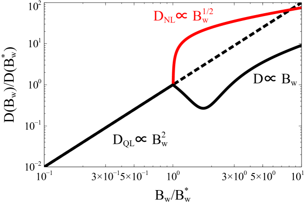
Figure 26: Schematic view of diffusion rate dependence on wave intensity. Intensity ${\cal B}_{w}^{*}$ corresponds to the threshold for nonlinear resonant interactions, $a=1$. See details in Frantsuzov et al. [2023].

6 Mapping technique for short wave-packets

The mapping technique is a more flexible approach than the kinetic equation (19), and this allows to make several generalizations for the inclusion of short wave packets. However, one of the main limitations for the description of short wave-packet systems, the absence of an analytical model for ${\cal S}(\gamma)$, cannot be overcome anyway. Thus, we should either use some synthetically generated ${\cal S}(\gamma)$ in mapping equations (25) or resort to a numerical integration of electron trajectories to determine the ${\cal S}(\gamma)$ profiles.

6.1 Simplified mapping and typical scalings

We start our consideration with the limit of very short wave-packets, when ${\cal S}(\gamma)$ can be approximated by Eq. (21), but the dynamics of wave-packets make it possible for electrons to interact resonantly with different wave amplitudes (and different $dB_{w}/d\lambda$ gradients) at any latitude. Note that the smallest wave-packet size (the shortest timescale of phase trapping) has been considered in Appendix C, while in the present section, we only consider short wave-packets with a size exceeding this minimum threshold size.

First, it is important to recall that nonlinear resonant interactions lead to significant energy drifts or jumps, and that such energy drifts and jumps cannot be accurately (fully) described within a diffusive framework, which intrinsically assumes very small and random individual energy changes, with zero mean value. Therefore, we focus here on a more general characteristic of the dynamic evolution of the electron distribution, common to both the quasi-linear and nonlinear regimes: the characteristic timescale of relaxation of the electron distribution toward its asymptotic steady-state. This asymptotic steady-state was indeed shown in Section 4.2 to be essentially the same state for both regimes. As will be demonstrated below, this common characteristic parameter will provide a way to approximately incorporate nonlinear effects in the diffusive framework.

Let us examine the characteristic timescale of the evolution of the electron distribution in a system with nonlinear wave-particle resonant interactions. Numerical and analytical solutions of Eq. (19) have shown that a plateau will ultimately be formed in the distribution function of electrons within the energy range of nonlinear resonant interactions, ${\cal S}\neq 0$. This implies that the electron distribution will tend toward a solution identical to the asymptotic solution of the Fokker-Planck diffusion equation. Therefore, we may assume that such evolution can on average be approximated by a diffusive transport, albeit with an effective nonlinear diffusion coefficient $D_{NL}$ different from the quasi-linear coefficient $D_{QL}\propto{\cal B}_{w}^{2}$. Such effective diffusion cannot describe all the peculiarities of nonlinear wave-particle interactions (e.g., the formation of transient electron populations at high-energies or the drift due to phase bunching), but it should provide a reasonable description of both the asymptotic (plateau) state of the electron distribution and of the characteristic timescale for reaching this asymptotic state. This effective nonlinear diffusion coefficient $D_{NL}$ should depend on wave intensity ${\cal B}_{w}^{2}$ and wave-packet size $\ell$, and for very small $\ell$ this coefficient should tend toward the scaling $D_{NL}\propto{\cal B}_{w}$ derived in Sect. 5.2.

6.1.1 Effective nonlinear diffusion

To develop the procedure of $D_{NL}$ derivation, let us start with the simple form of ${\cal S}(x)$ given by Eq. (21), with a multiplication factor $\delta_{0}^{5/4}$ (see Appendix C). We introduce the parameter $\kappa$ through the equation $\delta_{0}=\left({\cal B}_{w}/B_{0}\right)^{4\kappa/5}$. This parameter $\kappa$ is related to the maximum number of trapped particle periods, $N_{trap}$, during resonant interaction with a wave-packet, and a larger $\kappa$ corresponds to a smaller $N_{trap}$ (see Appendix C, and here below). We rewrite Eq. (21) as

$${\cal S}=\left({\cal B}_{w}/B_{0}\right)^{1/2+\kappa}\left({1-x{}^{2}}\right)^{5/4}$$ (31)

Figure 27 shows examples of trajectories given by this mapping and examples of the evolution of the particle distribution function $f(x)$. For $\kappa=0$, the trajectory is very similar to the trajectory displayed in Fig. 16(a), but for $\kappa=1/3$ we have smaller ${\cal S}\propto({\cal B}_{w}/B_{0})^{1/2+\kappa}=({\cal B}_{w}/B_{0})^{5/6}\ll({\cal B}_{w}/B_{0})^{1/2}$, which results in smaller $x$ changes due to bunching (longer intervals of $x$ decrease) and a smaller probability of trapping (rarer jumps with $x$ increase). Despite these differences, the evolution of the particle distribution $f(x)$ is quite similar, but it takes more time for $\kappa=1/3$. Figure 27(b,c) shows that after $100$ resonant interactions ($1000$ for $\kappa=1/3$) the initially localized $f(x)$ is transformed into a uniform distribution, in agreement with the asymptotic solution derived in Sect. 4.2 (see also Fig. 24(b)). Therefore, $\kappa$ regulates the time of $f(x)$ evolution, but does not change the main features of this evolution and its asymptotic solution.

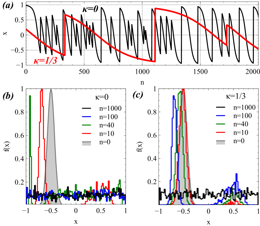
Figure 27: Panel (a) shows two examples of $x_{n}$ trajectories described by map (26) with ${\cal S}$ given by Eq. (31). Panels (b,c) show evolution of $f(x)$ distribution for two $\kappa$ values. Results are shown for ${\cal B}_{w}/B_{0}=10^{-3}$.

To characterize the timescale of the evolution of $f(x)$ as a function of $\kappa$, we numerically integrate a large ensemble of trajectories described by the map (31), for various values of $\kappa$. The initial $x_{0,i}$ values for the $i=0…N$ trajectories are uniformly distributed within the $[-1,1]$ range, and we calculate two characteristics:

$${\cal M}_{1}(n)=N^{-1}\sum_{i=0..N}\left(x_{n,i}-x_{0,i}\right)\;\;\;{\cal M}_{2}(n)=N^{-1}\sum_{i=0..N}\left(x_{n,i}-x_{0,i}\right)^{2}-{\cal M}_{1}^{2}(n)$$

where $x_{0,i}$ are initial $x_{i}$ values. Figure 28(a) shows ${\cal M}_{1}$ and ${\cal M}_{2}$ profiles for two $\kappa$ values: ${\cal M}_{1}$ is around zero and ${\cal M}_{2}$ first increases with the number of resonant interactions, and then saturates. This saturation means a full mixing of particles within the ${\cal S}(x)\neq 0$ domain (i.e., the formation of a plateau in the corresponding $f(x)$ distribution, without any $df/dx$ gradient). Before the saturation, the growing fragment of ${\cal M}_{2}$ can be fitted as

$${\cal M}_{2}(n)={\cal Q}n^{q}$$

and if $q\approx 1$, we may interpret the proportionality coefficient ${\cal Q}$ as a diffusion rate $D_{NL}$, because this coefficient describes the rate of increase of particle variance $d{\cal M}_{2}/dn$ during particle mixing. Note that, instead of being a local diffusion rate (that should depend on $x$), the coefficient $D_{NL}$ determined from the ${\cal M}_{2}(n)$ profile is a global system characteristics that is averaged over the entire $x$ range of ${\cal S}(x)\neq 0$. Because the particle dynamics include very large $x$ jumps (due to phase trapping; see Fig. 27(a)), this dynamics cannot be described locally by a diffusion, but the overall particle mixing within the entire $x$ range stills follows a diffusive-like behavior. Therefore, $D_{NL}$ may be considered as a global characteristic of nonlinear wave-particle interactions, corresponding to the inverse characteristic timescale of evolution of the electron distribution, and it can be compared with average quasi-linear diffusion rates. Figure 28(b) shows the $D_{NL}$ scaling with $\kappa$ and $\left({\cal B}_{w}/B_{0}\right)$: $D_{NL}\propto\left({\cal B}_{w}/B_{0}\right)^{1/2+\kappa}$, i.e., it is proportional to ${\cal S}$ magnitude.

To explain the scaling $D_{NL}\propto\left({\cal B}_{w}/B_{0}\right)^{1/2+\kappa}$, let us consider an ensemble of $N$ electrons with the same initial $x$ (i.e., with the same initial energy and $h$). The distribution of $\Delta x$ changes consists of two well separated populations: the most representative population contains almost all particles, $\sim N$, and have a finite $\langle x\rangle\propto{\cal S}\propto({\cal B}_{w}/B_{0})^{1/2+\kappa}$; this is the phase bunched population. A much smaller electron population contains only a tiny fraction $({\cal B}_{w}/B_{0})^{1/2+\kappa}$ of all resonant particles, $\sim N\Pi\sim N(B_{w}/B_{0})^{1/2+\kappa}$ where $\Pi=d{\cal S}/dx\propto{\cal S}$. This population is characterized by a finite $\langle\Delta x\rangle\sim O({\cal B}_{w}/B_{0})$. Such a large $x$ change is due to phase trapping. The dispersion of the entire distribution of $\Delta x$ is about

$$\left\langle{\left({\Delta x}\right)^{2}}\right\rangle\approx\left\langle{\Delta x}\right\rangle_{bunching}^{2}\frac{{N_{bunching}}}{N}+\left\langle{\Delta x}\right\rangle_{trapping}^{2}\frac{{N_{trapping}}}{N}$$

$$\sim\left({\frac{{{\cal B}_{w}}}{{B_{0}}}}\right)^{1+2\kappa}\cdot O\left(1\right)+O\left(1\right)\cdot\left({\frac{{{\cal B}_{w}}}{{B_{0}}}}\right)^{1/2+\kappa}\propto\left({\frac{{{\cal B}_{w}}}{{B_{0}}}}\right)^{1/2}$$

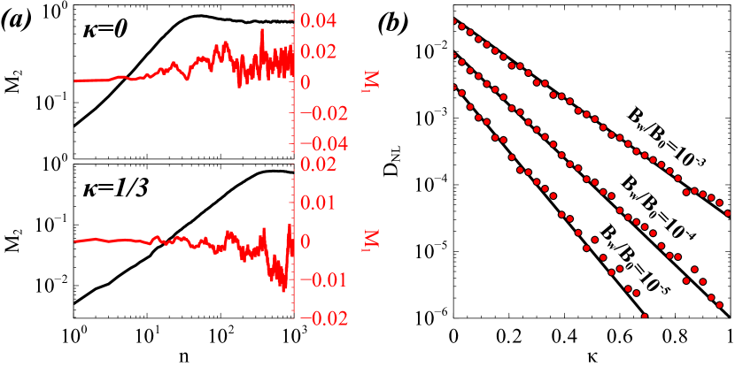
Figure 28: Panel (a) shows ${\cal M}_{1,2}$ profiles for two $\kappa$ values and ${\cal B}_{w}/B_{0}=10^{-3}$. Panel (b) shows $D_{NL}$ dependence on $\kappa$; fitting $D_{NL}\propto({\cal B}_{w}/B_{0})^{1/2+\kappa}$ is shown by black lines.

The parameter $\kappa$ (or equivalently, $\delta_{0}$) can be expressed through a more physical variable – the number of oscillations of phase trapped particles around the resonance, $N_{trap}$. For a small ${\cal S}$ in Eq. (31), the period of such oscillations can be written as $N_{trap}\sim\left({\cal B}_{w}/B_{0}\right)^{3\kappa/5-1/2}$ (see Appendix C). We use the normalized number of trapping periods ${\cal N}_{trap}=N_{trap}/N_{trap}^{\infty}$, where $N_{trap}^{\infty}\sim O(1)/\Omega_{tr}\sim\left({\cal B}_{w}/B_{0}\right)^{-1/2}$ is the number of periods in long wave-packets, where trapping and detrapping are determined by the latitudinal gradients of the background magnetic field and of the wave amplitude. Therefore, $N_{trap}/N_{trap}^{\infty}\sim\left({\cal B}_{w}/B_{0}\right)^{3\kappa/5}$ and $\left({\cal B}_{w}/B_{0}\right)^{\kappa}\sim{\cal N}_{trap}^{5/3}$. The effective diffusion rate $D_{NL}$ can be then written as

$$D_{NL}\sim\left({\cal B}_{w}/B_{0}\right)^{1/2+\kappa}\sim\left({\cal B}_{w}/B_{0}\right)^{1/2}{\cal N}_{trap}^{5/3}$$

For ${\cal N}_{trap}\to 1$, in the limit of long wave-packets, the effective nonlinear diffusion rate is $D_{NL}\sim\left({\cal B}_{w}/B_{0}\right)^{1/2}\propto{\cal B}_{w}^{1/2}$. The limit of intense but short wave-packets with $D_{NL}\sim\left({\cal B}_{w}/B_{0}\right)\propto{\cal B}_{w}$ can be reached for ${\cal N}_{trap}\sim\left({\cal B}_{w}/B_{0}\right)^{3/10}$ (or $N_{trap}\sim\left({\cal B}_{w}/B_{0}\right)^{-1/5}$). It is worth emphasizing that the short wave-packet approximation (or, in another words, the approximation of a symmetrical distribution of $\Delta x$ changes; see Fig. 25) provides a full analytical description of the transition from the classical quasi-linear diffusion rate $D_{QL}\propto{\cal B}_{w}^{2}$ to the strongly nonlinear effective diffusion rate $D_{NL}\propto{\cal B}_{w}$ (such that $D_{NL}>D_{QL}$), including all the numerical factors quantifying the diffusion rates. Note also that the effective nonlinear diffusion rate $D_{NL}\propto{\cal B}_{w}$ produced by intense short wave-packets (which represent the overwhelming majority of the observed chorus wave-packets in the Earth’s outer radiation belt) is larger than $D_{QL}$ because it includes a finite, important contribution from nonlinear interactions which hasten the evolution of the electron distribution, contrary to the ideal case of extremely short packets, briefly investigated in Section 5.2, where phase trapping and bunching strictly compensate each other, leaving only a purely diffusive transport at a rate lower than $D_{QL}\propto{\cal B}_{w}^{2}$ even in the high ${\cal B}_{w}$ range.

The effective nonlinear diffusion rate for long wave-packets, $D_{NL}\propto{\cal B}_{w}^{1/2}$ has a very large magnitude (see numerical test particle simulation results in Section 7), allowing $D_{NL}\propto{\cal B}_{w}^{1/2}$ to be much higher than $D_{QL}\propto{\cal B}_{w}^{2}$ over a wide range of ${\cal B}_{w}$ values. In a real system containing a large distribution of wave-packets of various sizes and peak amplitudes, the properties of this distribution will determine the actual magnitude of the effective nonlinear diffusion rate $D_{NL}$. However, because the scaling of the larger $D_{NL}$ with $B_{w}$ in the case of (rare) long packets is slower ($D_{NL}\propto{\cal B}_{w}^{1/2}$) than for the weaker $D_{NL}$ due to short packets ($D_{NL}\propto{\cal B}_{w}$), which is itself increasing more slowly with $B_{w}$ than the even weaker quasi-linear diffusion rate $D_{QL}\propto{\cal B}_{w}^{2}$, it is no surprise that the total effective nonlinear diffusion rate may be close to the quasi-linear rate $D_{QL}\propto{\cal B}_{w}^{2}$ extrapolated into the high ${\cal B}_{w}$ range. This may explain why quasi-linear simulations often manage to reproduce the observed electron flux dynamics in the radiation belt Thorne et al. [2013]; Li et al. [2014]; Glauert et al. [2018]; Mourenas, Artemyev, Agapitov, Krasnoselskikh & Li [2014]; Ma et al. [2018] even when the measured wave intensity exceeds the threshold for nonlinear wave-particle interactions Zhang, Thorne, Artemyev, Mourenas, Angelopoulos, Bortnik, Kletzing, Kurth & Hospodarsky [2018]; Zhang, Mourenas, Artemyev, Angelopoulos, Bortnik, Thorne, Kurth, Kletzing & Hospodarsky [2019].

6.1.2 Diffusion by multiple short wave-packets

The mapping (31) can successfully describe electron resonant interactions with a short wave-packet, but this interaction is assumed to take place within the entire energy range where ${\cal S}\neq 0$. This is a simplified case. In a more realistic situation, we deal with multiple short wave-packets. At a given time, each of these wave-packets covers only a small range of magnetic latitudes and, thus, will interact resonantly with electrons such that their energy is comprised within only a small portion of all the resonant energies at these latitudes. We consider a bounce period as an elementary time-step between electron resonant interactions that change their energy and pitch-angle. After each time-step, wave-packets will have significantly propagated, and each electron resonant interaction will occur with a new distribution of wave-packets along the magnetic field line. Therefore, we should include into the model (1) the probability for each electron to meet one wave-packet at the resonant latitude, (2) the corresponding limited range of resonant energies for each wave-packet. This limited energy range of actually resonant electrons represents a fraction $\chi<1$ of the total energy range of particles potentially reaching resonance with a wave packet over the full length of the magnetic field line.

Electron trapping by a short packet leads to a smaller energy change than trapping by an ideal infinitely long wave packet, because the electron is released from trapping faster, corresponding to a reduction of its energy change by a factor $\sim\chi$. If short wave packets are rare (not appearing in close succession) and occur only approximately once every bounce period, this corresponds to an additional reduction of the occurrence rate of resonant interaction by a factor $\sim\chi<1$, as compared with both the case of a close succession of short packets and the ideal case of infinitely long packets assumed in the preceding subsection.

Accordingly, let us consider a realistic situation where the magnitude of ${\cal S}\sim\left({\cal B}_{w}/B_{0}\right)^{1/2}$ remains the same, but the range of nonlinear resonant interactions shrinks. There are two kinds of systems with an total resonant range $x\in[-1,1]$, but where ${\cal S}$ is not equal to zero only for $x\in[-\ell,\ell]$, with $\chi=\sqrt{\delta_{0}}$. In systems of the first kind, we center ${\cal S}$ around a $\bar{x}_{n}$ randomly generated at each map iteration around $x_{n}$, i.e., for each iteration there is a finite change of $x_{n}$. This type of mapping mimics electron resonant interactions with a set of short wave-packets that would fill the entire magnetic field lines, but which cannot trap electrons for a long time because of the limited packet duration. Figure 29(a) shows observational examples of such a dense filling of the field-line by short wave packets.

In the system of the second kind, we center ${\cal S}$ around a randomly generated $\bar{x}_{n}$, but we do not control the position of $\bar{x}_{n}$ relative to $x_{n}$ and some map iterations can occur without any change of $x_{n}$ because $x_{n}$ is outside the ${\cal S}\neq 0$ range. This type of mapping mimics electron resonant interaction with rare short wave-packets propagating with a significant time separation. It corresponds to a situation where, during each bounce period, only one wave packet is present and many electrons reach the latitude of cyclotron resonance without encountering this intense packet there. Figure 29(b) shows observational example of such rarefied filling of a magnetic field-line by short wave packets.

For both systems, the mapping (31) can be rewritten as

$$x_{n+1}=x_{n}+\left\{{\begin{array}[]{*{20}c}{\bar{x}_{n}-2x_{n},}&{\xi\in\left[{0,\Pi}\right]}\\ {-{\cal S}_{n}\left({x_{n}}\right),}&{\xi\in\left({\Pi,1}\right]}\\ \end{array}}\right.$$ (32)

and

$${\cal S}_{n} = \left({\cal B}_{w}/B_{0}\right)^{1/2}\left({\chi^{2}-\left({x-\bar{x}_{n}}\right)^{2}}\right)^{5/4}$$

$$\Pi = \frac{{d{\cal S}_{n}}}{{dx}}=-\frac{5}{2}\left({x-\bar{x}_{n}}\right)\left({\cal B}_{w}/B_{0}\right)^{1/2}\left({\chi^{2}-\left({x-\bar{x}_{n}}\right)^{2}}\right)^{1/4}$$

where $\bar{x}_{n}=x_{n}+\chi\cdot R$ for the system of the first kind, and $\bar{x}_{n}=-1+\chi+2(1-\chi)\cdot R$ for the system of the second kind; here $R$ is a random number with a uniform distribution within $[-1,1]$ (note that for $\bar{x}_{n}=y_{n}+\chi\cdot R$ we also control that ${\cal S}\neq 0$ range does not cross $x\pm 1$ boundaries). An important property of both systems is that for small $\chi$, trapping is possible for any $x_{n}$ values, whereas for $\chi=1$ (the initial map given by Eq. (31)) trapping is possible only for $x_{n}<0$. Figure 29(c,d) shows a set of sample trajectories for each of the two kinds of systems. The rate of change of $x$ is going down as $\chi$ decreases, and this effect is stronger for the system of the second kind (Fig. 29(d)).

For these two kinds of systems, we set the range of $\chi$ and for each $\chi$ value we calculate ${\cal M}_{2}(n)$. Then we fit the growing fragment of ${\cal M}_{2}(n)$ by $D_{NL}n$. Fig. 29(e) shows the corresponding $D_{NL}$ dependence on $\chi$. For both systems, $D_{NL}$ scales with $\chi$ as $D_{NL}\sim\left({\cal B}_{w}/B_{0}\right)^{1/2}\chi^{\eta}$. But $\eta\approx 7/2$ for the system of the first kind, where resonances occur at each iteration, whereas $\eta\approx 9/2$ for the system of the second kind, where resonance occurrence is decreased by a factor $\chi\ll 1$. Taking into account that $\chi=\sqrt{\delta_{0}}$, we can write ${\cal N}_{trap}\sim\chi^{3/2}$. Therefore, for the scaling of $D_{NL}$ as a function of ${\cal N}_{trap}$ we have $D_{NL}\sim\left({\cal B}_{w}/B_{0}\right)^{1/2}\chi^{\eta}\sim\left({\cal B}_{w}/B_{0}\right)^{1/2}{\cal N}_{trap}^{2\eta/3}$ and $D_{NL}\sim\left({\cal B}_{w}/B_{0}\right)^{1/2}{\cal N}_{trap}^{2\eta/3}$. For $\eta=5/2$, this scaling allows to recover the scaling of the ideal case of electron interactions with infinitely long wave packets/waves present all the time along magnetic field lines: $D_{NL}\sim\left({\cal B}_{w}/B_{0}\right)^{1/2}{\cal N}_{trap}^{5/3}$. In the more realistic situation of short wave packets, two different kinds of systems are possible, corresponding to $\eta=7/2$ and $\eta=9/2$. For the system of the first kind, we get $D_{NL}\sim\left({\cal B}_{w}/B_{0}\right)^{1/2}{\cal N}_{trap}^{7/3}$. For the system of the second kind, we have $D_{NL}\sim\left({\cal B}_{w}/B_{0}\right)^{1/2}{\cal N}_{trap}^{3}$. The parameter ${\cal N}_{trap}$ depends on wave characteristics (dispersion, wave-packet size, and wave magnitude) and resonant electron characteristics. Although simplified scalings of this parameter with wave and electron characteristics can be derived analytically (see Figs. 28 and 29 and [Artemyev, Neishtadt, Vasiliev & Mourenas, 2021]), a more accurate (likely numerical) approach is needed to complete the quantification of the diffusion regimes for different wave amplitudes and wave coherence. Beside a fully numerical approach through test particle simulations, there are two promising directions for solving the problem of the dynamics of a large ensemble of resonant electrons. The first direction requires a significant modification of the mapping technique, with inclusion of realistic distributions of ${\cal B}_{w}^{2}$ and $\ell$. We discuss this approach in Section 6.2. The second approach requires incorporating a mixture of quasi-linear and nonlinear resonant effects, weighted by the ${\cal P}({\cal B}_{w},\ell)$ distribution, into the Fokker-Planck diffusion equation; we discuss this second approach in Section 7.

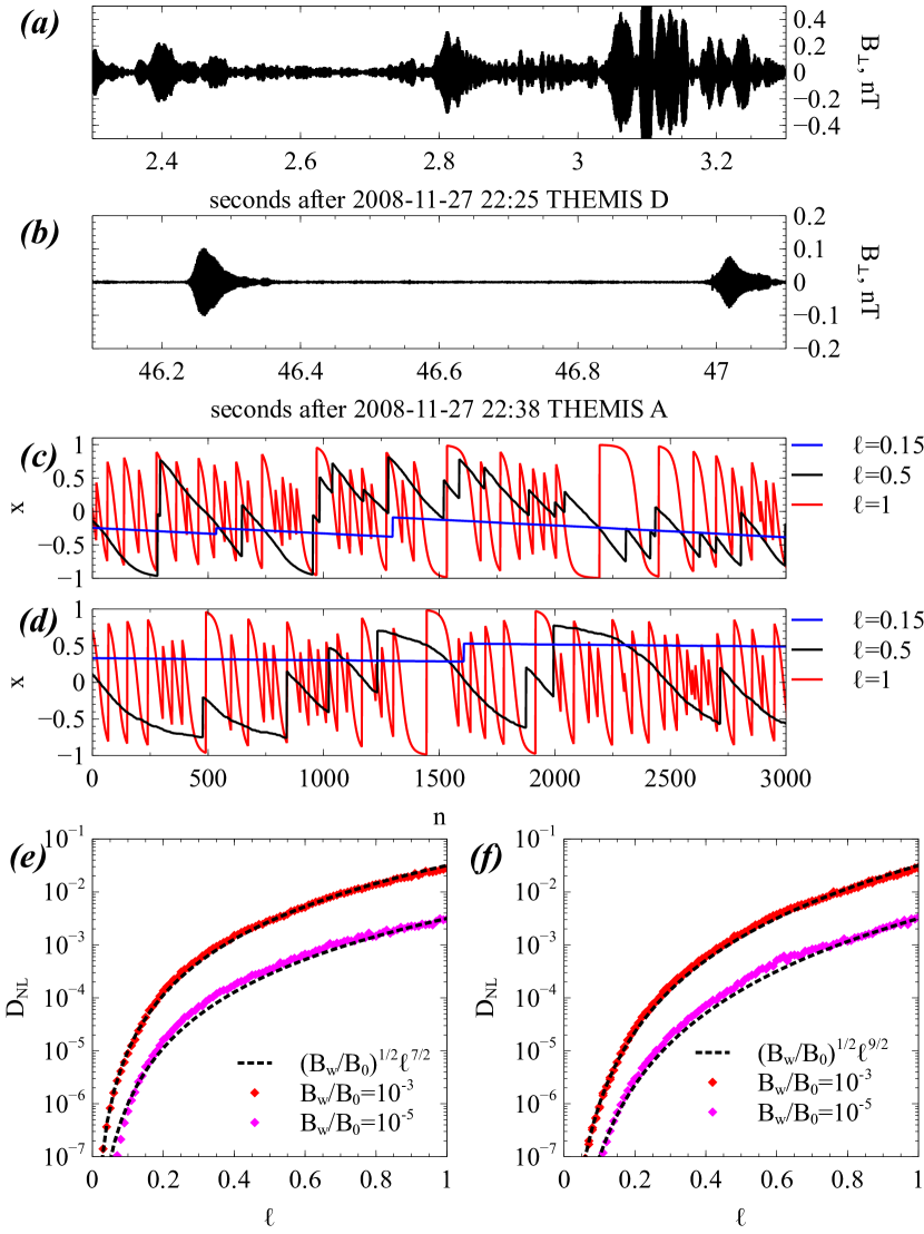
Figure 29: (a,b) show observational examples of dense and rarefied filling of a magnetic field field line by short wave-packets. Data are collected by THEMIS search-coil magnetometer Le Contel et al. [2008]. Details of these wave events can be found in Zhang, Agapitov, Artemyev, Mourenas, Angelopoulos, Kurth, Bonnell & Hospodarsky [2020]. Panels (c,d) show examples of trajectories $x(n)$ for the two types of models of mapping (32). Panel (e) shows the corresponding scaling of $D_{NL}=d{\cal M}_{2}/dn$ with $\chi$ for the two models of mapping.

6.2 Synthetic map

The mapping (32) is a simplified version of the realistic map describing electron resonant interaction with multiple different wave-packets. Although this simplified version does reproduce many peculiarities of such interactions, we may still generalize it to incorporate the observed distribution of wave characteristics, ${\cal P}(B_{w},\ell)$, as in examples shown in Figure 30(b) for field-aligned whistler-mode waves. This distribution shows the prevalence of short packets, but also demonstrates the existence of very long packets with $\ell>100$. Note that the method of wave-packet determination (i.e., the criterion used for identifying the wave-packet edges) can significantly affect the shape of the ${\cal P}(B_{w},\ell)$ distribution [see results in Zhang, Mourenas, Artemyev, Angelopoulos, Bortnik, Thorne, Kurth, Kletzing & Hospodarsky, 2019; Zhang et al., 2021]. Wave-packets for very oblique whistler-mode waves are generally shorter (compare panels (a) and (b) of Fig. 30) because their comparatively lower magnetic fields (corresponding to very high electric field amplitudes) are often closer to the noise level. The dimension of wave characteristics can be further increased by including wave frequency, ${\cal P}({\cal B}_{w},\ell)\to{\cal P}\left({\cal B}_{w},\ell,\omega/\Omega_{0}\right)$. Each bin of this distribution corresponds to a specific map, but in contrast to the $\ell\to\infty$ limit where such a map can be evaluated analytically (see Section 4.4), for an arbitrary $\ell$ there is no analytical model of wave-particle resonant interactions. Therefore, this approach should rely on test-particle simulations, and the results of such simulations should be either incorporated into the Green function approach Hsieh et al. [2020, 2022], or somehow used for an improved mapping.

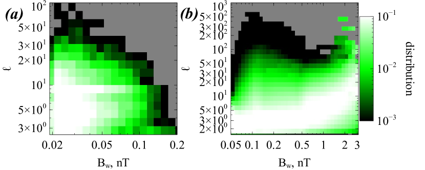
Figure 30: Distributions of wave-packets amplitudes and sizes for very oblique (a) and field-aligned (b) whistler-mode waves ($L$-shell$\in[6,10]$ for very oblique waes, THEMIS statistics; $L$-shell$\in[4,6]$ for parallel waves, Van Allen Probe statistics [see details of dataset in Zhang, Mourenas, Artemyev, Angelopoulos, Bortnik, Thorne, Kurth, Kletzing & Hospodarsky, 2019]). All levels of geomagnetic activity are included.

The idea of incorporating such wave-packet distributions into the mapping technique has been proposed in Tonoian et al. [2023]; Shi et al. [2023], and can be named the synthetic map approach. This approach consists in the construction of a combined map

$$\hat{M}=\sum\limits_{{\cal B}_{w},\ell,\omega}{P\left({{\cal B}_{w},\ell,\omega}\right)\hat{m}}$$ (33)

where $\hat{m}$ is the mapping described by Eq. (32) with the

$${\cal S}_{{\cal B}_{w},\ell,\omega}=C_{{\cal B}_{w},\ell,\omega}\left({\cal B}_{w}/B_{0}\right)^{1/2}\left(\chi^{2}-(x_{n}-x)^{2}\right),$$

where $=C_{{\cal B}_{w},\ell,\omega}$, $\chi$, and the probability distribution of ${\cal P}(x_{n})$ have to be determined through test particle simulations. Such simulations (for fixed ${\cal B}_{w}$ ,$\ell$ ,$\omega/\Omega_{0}$) provides the probability distribution function of particle energy changes, and the main elements of ${\cal S}_{{\cal B}_{w},\ell,\omega}$ model can be derived from this distribution – see schematic view in Fig. 31(a). The maximum energy change due to trapping determines the parameter $\chi$, which should be proportional to the wave-packet size parameter $\ell$ (see Fig. 22(b)). The magnitude of negative energy changes due to phase bunching determines the parameter $C_{{\cal B}_{w},\ell,\omega}$, which denotes the normalized magnitude of the area ${\cal S}$. The relative number of test particles such that their energy does not change in the first resonant interaction, due to an absence of wave-packet at the latitude of resonance, determines the distribution ${\cal P}(x_{n})$ [see details in Tonoian et al., 2023]. Therefore, even a quite roughly reproduced (due to limited statistics from test particle simulations) probability distribution of electron energy changes may allow to reproduce the main mapping characteristics and to construct a synthetic map. Figure 31(c) shows an example of such a synthetic map, constructed to reproduce the numerically obtained distribution of electron energy changes from Fig. 31(c). Although the synthetic map is simplified and omits many details of this distribution, the application of this map for the simulation of the dynamics of an ensemble of electrons shows very similar results to what can be obtained directly from test particle simulations (e.g., compare panels (d) and (e) in Fig. 31). The general dynamics of the electron energy distribution for this simulation shows an increase of energetic particle population due to trapping, but because we deal with an ensemble of short wave-packets, the formation of the plateau in the distribution function takes a much longer time than for simulations with long wave-packets.

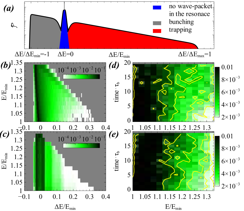
Figure 31: Panel (a) provdies a schematic view of the construction of the $\hat{m}$ mapping using the numerically evaluated distribution of energy changes. Note that we normalize electron energy to the minimum energy, $E_{\min}$, of the range where the nonlinear resonant interactions are possible. Panels (b, c) show the numerically determined 2D probability distribution ${\cal P}(E/E_{\min},\Delta E/E_{\min})$, as fitted by a sum of $\hat{m}$ maps. Panels (d, e) show the evolution of the electron distribution function obtained directly from test particle simulations and, indirectly, using the mapping technique with the synthetic map shown in panel (c). Details of this demonstration of the usefulness of the synthetic map can be found in Tonoian et al. [2023].

The method of construction of a synthetic map resembles a general decomposition technique where the results of multiple different processes (bunching and trapping by wave-packets having different amplitudes and sizes) is expressed as a linear sum of elementary processes, each of them being described by a simple model (e.g., the mapping model (32)). Such a decomposition requires a minimization of the difference between ${\cal P}(\Delta E)$ derived numerically and obtained from Eq. (33). Numerical schemes for this minimization are not yet well developed (Tonoian et al. [2023] used a quite simplified form of determination of the parameters of Eq. (32) shown in Fig. 31) and, therefore, the synthetic map approach has not been thoroughly investigated yet. However, this approach looks quite promising for complicated (realistic) systems, and it would be worth generalizing and developing it in the future.

6.3 SDE versus mapping

The mapping approach utilizes the probability distribution function of electron resonant energy changes, ${\cal P}(\Delta E)$, and thus, it is quite similar to the more widespread stochastic differential equation (SDE) approach, which is mostly used for simulations of the purely diffusive regime of wave-particle interactions. The basic idea of SDE is that, instead of directly solving the Fokker-Planck equation, one can write and solve the corresponding Ito stochastic differential equations of quasi-particle trajectories Tao et al. [2008]; Zheng et al. [2014]:

$$\boldsymbol{p}(t+\Delta t)=\boldsymbol{p}(t)+\boldsymbol{\mu}(\boldsymbol{p}(t),t)\Delta t+\boldsymbol{\sigma}(\boldsymbol{p}(t),t)\boldsymbol{dW_{t}}$$ (34)

where $\Delta t$ is the time step over which we calculate the change of $\boldsymbol{p}=(p_{\parallel},p_{\perp})$, $\boldsymbol{\mu}(\boldsymbol{p}(t),t)$ is a $2$-dimension vector of the drift coefficient, $\boldsymbol{\sigma}(\boldsymbol{p}(t),t)$ is a $2\times 2$-dimension matrix related to the diffusion coefficients written in such a way that $\hat{D}_{pp}=\frac{1}{2}\boldsymbol{\sigma}\boldsymbol{\sigma}^{T}$, $\hat{D}_{pp}$ is a $2\times 2$ matrix of diffusion coefficientsLyons & Williams [1984]; Schulz & Lanzerotti [1974]; Albert [2018], $\boldsymbol{W_{t}}$ is a $N$-dimension standard Wiener process; $\boldsymbol{dW_{t}}=\sqrt{\Delta t}\boldsymbol{N}$, where $\boldsymbol{N}$ is a vector of standard normal random values, $N_{i}\sim N(0,1)$.

The term quasi-particles means that we do not directly integrate the equations of motion, but treat the change of $\boldsymbol{p}$ as a stochastic process and approximate it by the equation (34). As a result, two quasi-particles having equal initial conditions $\boldsymbol{p}_{0}$ may have different trajectories $\boldsymbol{p}(t)$ (in the numerical integration of the equation (34), one can fix the seed of the pseudo random number generator to preserve the sequence of random numbers and make the results repeatable). We can examine electron distributions in the energy space, and thus the Ito equation (34) can be rewritten in the following form

$$E(t+\Delta t)=E(t)+\mu_{E}\left(E(t)\right)\Delta t+\sqrt{2D_{EE}\left(E(t)\right)}dW_{t}$$ (35)

This equation describes energy evolution for a fixed $h$ given by Eq. (4), i.e., for a monochromatic wave we may reduce the energy, pitch-angle evolution to the energy evolution only and calculate pitch-angle changes from $h$ conservation. In the more general case of a wave spectrum, there are three diffusion rates (energy, pitch-angle, and mixed energy-pitch-angle) and, thus, we would need to solve a system of equations for energy and pitch-angle evolution [see detail in Tao et al., 2008]. Note also that if we rewrite the Fokker-Planck equation in terms of energy, additional coefficients of variable transformation from velocity(momentum) to energy and pitch-angle (Lamé coefficients) should be added [e.g., Glauert & Horne, 2005], but the Ito equation will still have the same form. Equation (35) is quite similar to the mapping equations (compare with Eqs. (26)), but instead of a more complicated probability distribution function containing phase trapped and bunched populations, this equation utilizes a Gaussian distribution of random energy jumps.

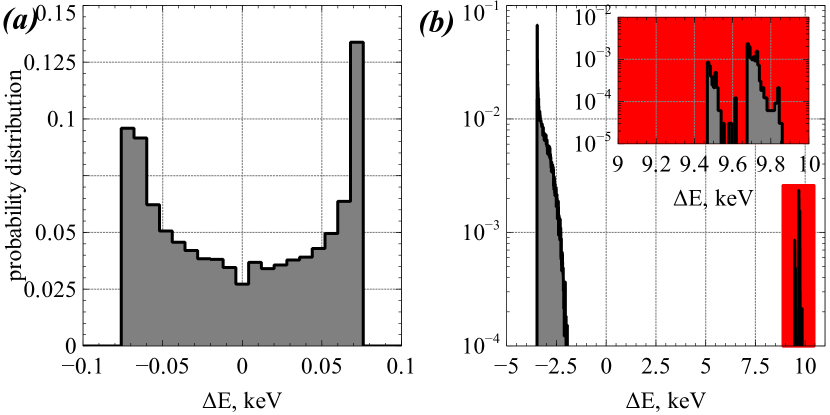
Figure 32: Two examples of ${\cal P}(\Delta E)$ distributions for low-amplitude waves with ${\cal B}_{w}/B_{0}=10^{-4}$(a) and intense waves with ${\cal B}_{w}/B_{0}=10^{-3}$(b). In panel (b) the red insert zooms in on ${\cal P}(\Delta E)$ for trapped particles. System parameters are: $\omega/\Omega_{0}(0)=0.3$, $L=5$, $h=1.5$, field-aligned waves [see details in Lukin et al., 2024].

In this Section, we shall compare three methods (test particles, SDE, and mapping) to simulate the evolution of the electron distribution function, and these three methods are expected to give the same results for small wave amplitudes, when wave-particle resonant interactions are quasi-linear. The test particles approach is expected to be more precise, because it does not rely on a constructed $\Delta E$ distribution and it is based on the full set of equations of motion. The main advantage of SDE and mapping techniques is their computational efficiency in long-term simulations. Therefore, one can accept a lower accuracy of SDE and mapping, provided that they still describe the main features of the evolution of the electron distribution and that their results statistically reproduce the results from direct test particle simulations. Figure 33(a) shows the evolution of the electron distribution function for a small wave amplitude ($\left({\cal B}_{w}/B_{0}\right)=10^{-4}$): we show the initial distribution and the distributions obtained by three methods after $\sim 100$ bounce periods (see figure caption for details). Without nonlinear resonant interactions, both SDE and mapping technique show results consistent with the test particle simulation. In this case, the evolution is diffusive (as expected from quasi-linear theory) and shows a spread of the initially localized electron phase space density peak. The difference between SDE and the test particle simulation, most clearly seen around $E\sim 420$ keV, is due to an overestimation of the diffusion coefficients. We evaluate diffusion coefficients as half of the variance of $\Delta E$ distributions, and thus we assume that $\Delta E$ distributions are symmetric relative to their mean value. However, even in the case of low-amplitude waves (see, e.g., Figure 32(a)) this assumption may not work, leading to an overestimation of the diffusion rate. The mapping technique does not require any assumptions about $\Delta E$ distributions and, therefore, it performs better even in the case of low-amplitude waves.

Figure 33(a) shows that for small wave amplitudes, all three methods, SDE, mapping, and test particle simulations, provide the same evolution of the electron distribution function. This results underlines that the mapping technique is equivalent to SDE approach for the quasi-linear regime. Moreover, for such amplitudes the details of the ${\cal P}(\Delta E)$ distribution are not important: despite the fact that the distributions ${\cal P}(\Delta E)$ from Fig. 32(a) are not Gaussian, their dispersion well describes the electron dynamics due to a very large number of resonant interactions. This is a consequence of the Central limit theorem, which states that the mean value of weakly correlated variables is normally distributed as long as the sample size is large enough, whatever the probability distribution of these variables Elliott [1980]; Dudley [2014]. Therefore, we should not care too much about describing the fine details of the probability distributions of energy changes, but rather focus on their main characteristics ($\Delta E$ range, mean value, etc.).

Figure 33 (b) shows the evolution of the electron distribution function for a large wave amplitude ($\left({\cal B}_{w}/B_{0}\right)=10^{-3}$): we show the initial distribution and the distributions obtained by test particle simulations and by the mapping technique after $\sim 100$ bounce periods (see figure caption for details). For such intense waves, the SDE approach becomes fully inapplicable, but we can still compare the results from test particle simulations and from the mapping technique. The mapping technique accounts for nonlinear resonant interactions (e.g., phase trapping) and describes well the evolution of electron distribution. After several wave-particle resonant interactions, the main electron population propagates to lower energies due to the phase bunching, while a small population becomes trapped by waves and gains energy. During the drift of the main population toward smaller energy, the probability of particle trapping increases (see Figure 32(b)) and more particles become trapped and accelerated. Accelerated particles are transported to latitudes of resonance where phase trapping is not possible anymore, and thus, these particles start losing their energy due to phase bunching. Around the time when the main population (at the initial peak of electron phase space density) reaches the left boundary of the allowed energies, the processes of phase bunching and phase trapping statistically compensate each other. This results in the formation of a plateau in the distribution function; this moment is shown in Fig. 33(b). Such an evolution of the electron distribution is consistent with theoretical predictions for the system with multiple nonlinear resonances (see Section 4.2 and Artemyev, Neishtadt & Vasiliev [2019]).

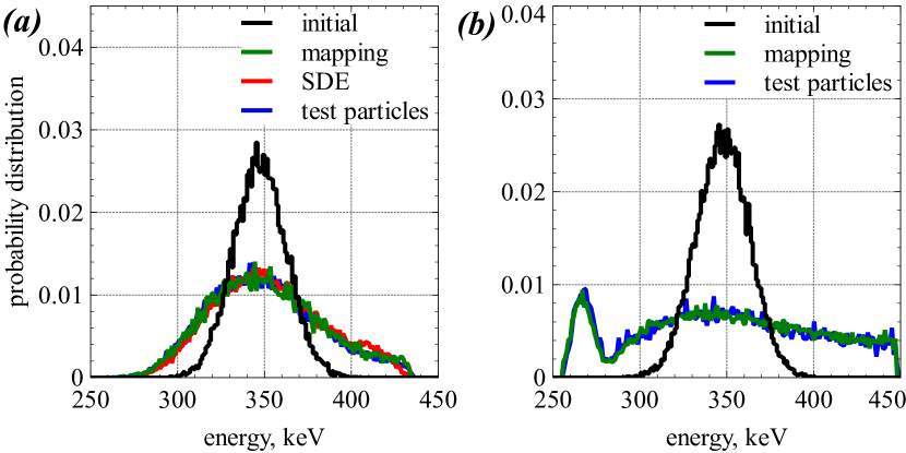
Figure 33: Two examples of evolution of electron distribution function, evaluated using different techniques, for low-amplitude waves with ${\cal B}_{w}/B_{0}=10^{-4}$(a) and for intense waves with ${\cal B}_{w}/B_{0}=10^{-3}$(b). System parameters are given in the caption of Fig. 33, the typical bounce period of electrons is $\tau_{b}\approx 0.7$s, and results are shown after $1100$ s of real time [see details in Lukin et al., 2024].

7 Incorporation of nonlinear resonant interactions into radiation belt models

The currently existing radiation belt models can be formally separated into two classes: test particle simulations in the global electromagnetic fields provided by MHD models, and solvers of the Fokker-Planck diffusion equations [see reviews in Shprits, Subbotin, Meredith & Elkington, 2008; Shprits, Elkington, Meredith & Subbotin, 2008]. Let us discuss the possible approaches for an incorporation of nonlinear resonant interactions into such existing models.

We start with test-particle simulation models, which build on advances in high-resolution global MHD simulations Elkington et al. [2004]; Hudson et al. [1999, 2012]. These models reproduce well many important details of energetic electron injections into the inner magnetosphere by fast plasma flows Sorathia et al. [2020], losses across the realistic dynamical magnetopause Hudson et al. [2014]; Sorathia et al. [2017], and radial transport by ultra-low-frequency (MHD) waves Hudson et al. [2015]; Sorathia et al. [2018]. A quite obvious deficiency of such models is the absence of any wave-particle interaction effects corresponding to electron scattering by whistler-mode (and any other non-MHD mode) waves. This issue may be resolved if test electron trajectories can be evaluated within the SDE approach, i.e., wave-particle interactions can be included as perturbations of electron dynamics for prescribed quasi-linear diffusion coefficients Chan et al. [2023]. Although this combined approach (test particle trajectories in MHD field and SDE for wave-particle interaction effects) is still under construction, we can suggest that it can be further generalized. The inclusion of nonlinear resonant effects can be performed by changing the probability distribution of electron energy/pitch-angle changes from the Gaussian one (describing diffusion) to a more complicated form including phase bunching and phase trapping effects. Section 6.3 describe such a generalization, which formally consists in replacing the SDE approach by the mapping technique [see also Artemyev, Neishtadt & Angelopoulos, 2022].

Finally, let us discuss the inclusion of nonlinear effects into existing radiation belt models based on Fokker-Planck diffusion equations. The numerical scheme of these models cannot be easily generalized for solving equations with integral operators, and it looks more reasonable to include nonlinear effects in the form of a renormalization of diffusion rates. Sections 6.1.1, 6.1.2 show that over the long term, electron interactions with intense waves indeed result in an effective nonlinear diffusion, with a nonlocal diffusion rate, $\tilde{D}_{NL}$, which represents the rate of electron mixing in the energy, pitch-angle domain of ${\cal S}\neq 0$. Such effective diffusion rates can be calculated for realistic wave-packet distributions in two regimes: for realistically high wave amplitudes, and for very small wave amplitudes, ${\cal B}_{w,small}$. The second regime will mimic quasi-linear diffusion and provide an estimate of the corresponding nonlocal mixing rate, $\tilde{D}_{QL}$. This rate can be further renormalized to the actual wave amplitude, $\tilde{D^{*}}_{QL}=\tilde{D}_{QL}\cdot\left({\cal B}_{w}/{\cal B}_{w,small}\right)^{2}$. The ratio of these rates can be considered as a normalized factor $R=\tilde{D}_{NL}/\tilde{D^{*}}_{QL}$ indicating the relative contribution of nonlinear effects. Figure 34(a) shows examples of $R$ dependencies on wave amplitude ${\cal B}_{w}$, in the case of short ($\ell=10$) and long ($\ell=300$) wave packets. For sufficiently small ${\cal B}_{w}$, there is no contribution from nonlinear effects, and for both $\ell$ values we have $R\approx 1$. As the wave amplitude ${\cal B}_{w}$ increases, the contribution of nonlinear effects increases, providing a larger $R$. This $R$ increase is stronger for longer wave-packets, due to a more important contribution of phase trapping into $\tilde{D}_{NL}$.

The coefficients $\tilde{D}_{NL}$ and $\tilde{D^{*}}_{QL}$ can be derived for different wave amplitudes and wave-packet sizes, and then averaged over the ${\cal P}({\cal B}_{w},\beta)$ distribution. Such averaging will provide the weighted factor $\langle R\rangle$ that should depend on the geomagnetic activity level, since ${\cal P}$ varies with geomagnetic activity (see Fig. 30). This factor can be determined for some energy, pitch-angle domains (roughly corresponding to ${\cal S}\neq 0$ domains for different constants $h$ given by Eq. (4)). Figure 34(b) shows examples of $\langle R\rangle$ evaluated for several electron energies such that $h$ remains constant. The factor $\langle R\rangle$ weakly increases with geomagnetic activity, but it varies significantly with energy. Depending on the specific procedure of $\tilde{D}_{NL}$ averaging over the distribution of wave-packet sizes and amplitudes, $\langle R\rangle$ can vary from $1.5$ up to $6$ for $100$ keV, whereas for $1$ MeV $\langle R\rangle$ can vary between $1.1$ and $1.5$ [see details in Artemyev, Mourenas, Zhang & Vainchtein, 2022]. By definition, $\langle R\rangle$ is determined from the statistics of $I_{x}$ variations. Therefore, this factor is equally applicable to pitch-angle and energy diffusion, i.e., the derived $\langle R\rangle$ will increase the rate of electron acceleration and precipitation.

Figure 34: (a) $R$ as a function of ${\cal B}_{w}$ in the case of short ($\ell=10$) and long ($\ell=300$) wave-packets. (b) $\langle R\rangle$ coefficient for two typical energies and two datasets of whistler-mode waves-packets (red and blue) [see details in Artemyev, Mourenas, Zhang & Vainchtein, 2022].

Figure 34 shows $\langle R\rangle$ for intermediate equatorial pitch-angles at $\sim 100$ keV and for small pitch-angles at $\sim 1$ MeV. Simulations for a multiple pitch-angle, energy domains provide a set of $\langle R\rangle$ values that can be fitted by a function of energy and pitch-angle. The coefficients of such fitting depend on properties of the ${\cal P}({\cal B}_{w},\beta)$ distribution. In particular, the relative contribution of long wave-packets in realistic situations is largely determined by the definition of the wave-packet edge, i.e., by the chosen method of determination of the wave-packet length in statistical observations Artemyev, Mourenas, Zhang & Vainchtein [2022]; Zhang, Thorne, Artemyev, Mourenas, Angelopoulos, Bortnik, Kletzing, Kurth & Hospodarsky [2018]; Zhang, Mourenas, Artemyev, Angelopoulos, Bortnik, Thorne, Kurth, Kletzing & Hospodarsky [2019]; Zhang, Mourenas, Artemyev, Angelopoulos, Kurth, Kletzing & Hospodarsky [2020].

For instance, if the wave-packet length is calculated between two consecutive minima of $B_{w}$ below $\sim 50$ pT but above $10$ pT Artemyev, Mourenas, Zhang & Vainchtein [2022]; Zhang, Mourenas, Artemyev, Angelopoulos, Kurth, Kletzing & Hospodarsky [2020], ${\cal P}({\cal B}_{w},\beta)$ contains a significant fraction of long wave-packets, and nonlinear effects (phase trapping) significantly amplify electron mixing in the phase space. Then, we can use

$$\left\langle R\right\rangle\approx 1+A\cdot\frac{{1+\sin\alpha_{eq}}}{{1+\left({E/E_{0}}\right)}}$$

where $E_{0}\approx 50$ keV and $A\approx 7$, so that $\left\langle R\right\rangle\approx 3$ for $\alpha_{eq}=0$ and $\left\langle R\right\rangle\approx 5.6$ for $\alpha_{eq}=\pi/2$ for $100$ keV, whereas $\left\langle R\right\rangle\approx 1.3$ for $\alpha_{eq}=0$ and $\left\langle R\right\rangle\approx 1.7$ for $\alpha_{eq}=\pi/2$ for $1$ MeV.

If the fraction of long wave-packets is reduced in ${\cal P}({\cal B}_{w},\beta)$, nonlinear effects are also reduced. For example, if we now assume that when the wave amplitude reaches one half of the packet peak amplitude, the wave phase fluctuations Santolík et al. [2014]; Hanzelka et al. [2020] destroy nonlinear resonances, then the wave-packet size distribution will contain only a small population of long packets Artemyev, Mourenas, Zhang & Vainchtein [2022]; Zhang, Mourenas, Artemyev, Angelopoulos, Bortnik, Thorne, Kurth, Kletzing & Hospodarsky [2019]. Under such an assumption, we get $A\approx 3.5$, so that $\left\langle R\right\rangle\approx 2.2$ for $\alpha_{eq}=0$ and $\left\langle R\right\rangle\approx 3.3$ for $\alpha_{eq}=\pi/2$ for $100$ keV, whereas $\left\langle R\right\rangle\approx 1.17$ for $\alpha_{eq}=0$ and $\left\langle R\right\rangle\approx 1.3$ for $\alpha_{eq}=\pi/2$ for $1$ MeV.

To demonstrate the applicability of the proposed approach, which consists in the introduction of a renormalization factor $\langle R\rangle$, we consider a case study during the 31 August 2019 - 01 September 2019 storm [see details of this event in Hudson et al., 2021; Nasi et al., 2022]. Figure 35 shows examples of electron phase space density (PSD) derived from measurements of Van Allen Probe A MagEIS (for $\mu=1000$ MeV/G) and REPT (for $\mu=4000$ MeV/G) instruments [Claudepierre et al., 2021; Blake et al., 2013; Baker et al., 2013]. The fast, localized (in $L^{*}$ evaluated with the TS05 [Tsyganenko & Sitnov, 2005] magnetic field model) increase in phase space density indicates an effective, local acceleration via wave-particle resonant interactions [Chen et al., 2007; Thorne et al., 2013]. As an example, we analyze the electron acceleration at $L^{*}=4.2$, where the phase space density increased $\sim$20-fold from 6:35 UT to 11:10 UT on 01 September (Figure 35b).

During this event, the characteristics of quasi-parallel whistler-modes wave and cold plasma are available from measurements of Van Allen Probe A ($MLT\in[9,15]$) and ERG ($MLT\in[3,9]$) [see details of missions in Mauk et al., 2013; Miyoshi et al., 2017]. We use background magnetic field measurements from the Magnetic Field Experiment Matsuoka et al. [2018] at $8$-second resolution, and high resolution electric and magnetic field wave spectra from the Onboard Frequency Analyzer [see Matsuda et al., 2018] onboard on the Plasma Wave Experiment Kasahara, Kasaba, Kojima, Yagitani, Ishisaka, Kumamoto, Tsuchiya, Ozaki, Matsuda, Imachi, Miyoshi, Hikishima, Katoh, Ota, Shoji, Matsuoka & Shinohara [2018]. We also utilize measurements from the Electric and Magnetic Field Instrument Suite and Integrated Science Waves instrument [Kletzing et al., 2013] providing all components of the wave electric and magnetic fields. To exclude measurements within the plasmasphere, we use the electron plasma density inferred from the upper hybrid resonance frequency line in the $10-400$ kHz range for Van Allen Probes [Kurth et al., 2015] and in the 10 kHz - 10 MHz range for ERG [Kumamoto et al., 2018]. To obtain the full MLT coverage of waves and total electron density, we use measured wave intensities to scale an empirical wave model Meredith et al. [2012], whereas ambient plasma measurements are used to scale global empirical density models Sheeley et al. [2001]; Denton et al. [2006]. Measurements by Van Allen Probe A and ERG are combined at $L^{*}\sim 4.2$, binned and interpolated in time to an 1-h resolution, and then we calculate diffusion rates at each $1$-h time step (see Fig. 36).

We use classical quasi-linear diffusion coefficients, without or with the nonlinear renormalization factor $\langle R\rangle>1$, to solve the bounce-averaged Fokker-Planck equation [Lyons et al., 1972; Glauert & Horne, 2005] using University of California, Los Angeles (UCLA) full diffusion code [see Ni et al., 2008; Ni, Thorne, Meredith, Shprits & Horne, 2011; Ma et al., 2015, 2018]. The wave normal angle distributions and latitude ranges at different MLT sectors are from [Thorne et al., 2013]. After the diffusion coefficients are calculated, we perform 2D Fokker Planck simulation Ma et al. [2012] to examine the electron phase space density evolution due to chorus waves. Figure 37 compares the observed electron flux dynamics (dashed) and the simulation results (solid). The first simulation, which includes only pure quasi-linear diffusion (with $\langle R\rangle=1$), clearly underestimates the electron acceleration rate above $1$ MeV, where the simulation fails to reproduce the observed rapid $\sim 5$-hour electron flux increase (Figure 37a). The second simulation, with renormalized diffusion rates (with $\langle R\rangle>1$), leads to a much better agreement between the modelled increase of relativistic electron fluxes and actual spacecraft observations (Figure 37b). This benchmark comparison therefore confirms the validity of our approach for incorporating the effects of nonlinear resonant interactions into classical Fokker-Planck simulations of energetic electron dynamics. It also underlines the importance of such generalized radiation belt models for an accurate description of electron dynamics in the presence of intense wave-packets [see Kondrashov et al., 2024, for another example of the application of the same approach].

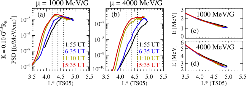
Figure 35: (a, b) Evolution of the electron phase space density for two magnetic moment values with a fixed second adiabatic invariant, as derived from Van Allen Probe A measurements on 01 September 2019, and (c, d) the corresponding electron energy as a function of $L^{*}$. Colors represent the times when Van Allen Probe A was at $L^{*}=4.2$. The phase space density is derived with the TS05 [Tsyganenko & Sitnov, 2005] magnetic field model.

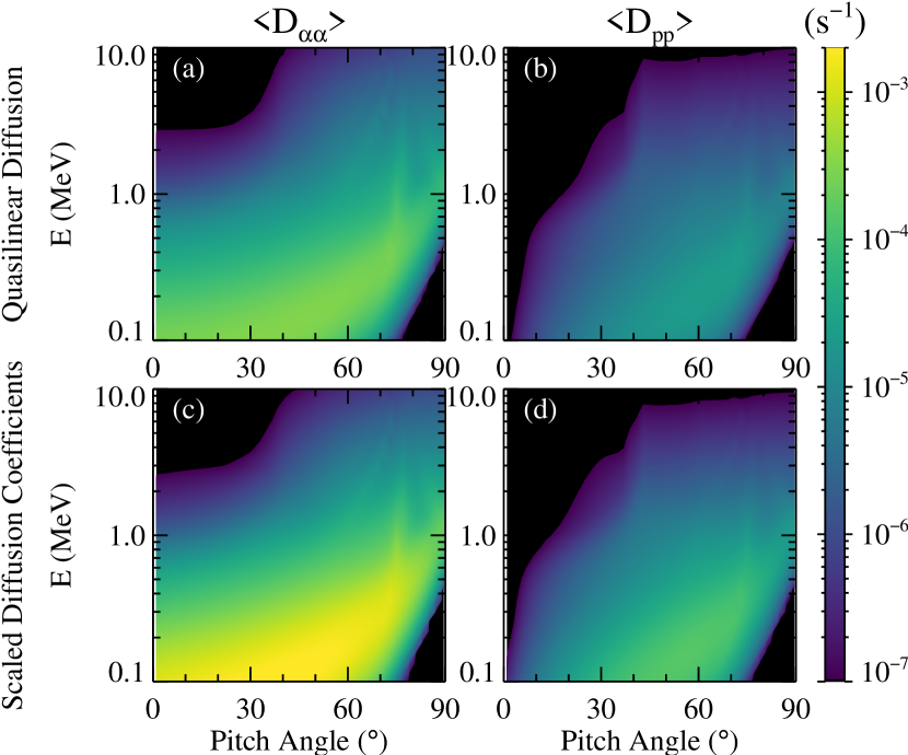
Figure 36: Time, MLT and bounce-averaged pitch-angle (left) and momentum (right) diffusion rates for electron acceleration at $L^{*}=4.2$ observed from 6:35 UT to 11:10 UT on 01 September 2019 [see equations of quasi-linear diffusion rates in Glauert & Horne, 2005]; (a, b) quasi-linear diffusion rates $D_{QL}$ (top), and (c, d) rescaled rates $\langle R\rangle D_{QL}$ (bottom) based on the multiplication factor $\langle R\rangle>1$ obtained for the wave model in Fig. 34.

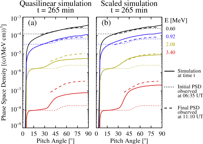
Figure 37: Evolution of pitch-angle distributions of electron PSD at different energies at $L^{*}=4.2$: solid lines show simulation results after 265 min in the simulation, dotted lines show the PSD observed at 06:35 UT (used as the initial condition), and dashed lines show the PSD observed at 11:10 UT (used as the final state to verify the model results). (a) Simulation results using quasi-linear diffusion rates, and (b) simulation results obtained with the rescaled (using a renormalization factor $\langle R\rangle>1$) diffusion rates (see Fig. 36).

8 Discussion and Conclusions

8.1 Effects beyond the classical resonance model

For simplicity, we may define wave-particle resonant interactions as processes satisfying the cyclotron resonance condition with $O(1)$ accuracy in the ${\cal B}_{w}/B_{0}$ parameter:

$$\frac{{p_{\parallel}}}{{m_{e}}}k_{\parallel}-\gamma\omega+\Omega_{0}=0$$ (36)

Then, we can discuss several effects going beyond this definition, calling them nonresonant, although some of them can still be called nonlinear resonant effects. Many of these effects have been investigated in details for electromagnetic ion cyclotron waves Grach & Demekhov [2018a, 2020]; Grach et al. [2022]; Bortnik et al. [2022] and for magnetosonic waves Bortnik & Thorne [2010]; Bortnik et al. [2015], whereas the importance of these effects for whistler-mode waves is not always obvious. However, to offer a comprehensive picture of nonlinear interactions, we discuss below all these effects, as applied to electron resonant interaction with whistler-mode waves.

Anomalous phase trapping

One example of such effects has already been considered in Section 3, where we discussed wave-particle interactions for small pitch-angle electrons, when the term $\propto({\cal B}_{w}/B)/\sqrt{I_{x}}$ should be included into the equation of phase variation

$$\frac{{p_{\parallel}}}{{m_{e}}}k_{\parallel}-\gamma\omega+\Omega_{0}=\sqrt{\frac{{2\Omega_{0}}}{{Im_{e}c^{2}}}}\frac{{eB_{w}}}{k}\cos\zeta$$ (37)

Such a generalization results in a new type of resonant dynamics, where electrons appear to be phase trapped by default; the so-called autoresonance effect Fajans & Frièdland [2001]; Friedland [2009]; Neishtadt et al. [2013]; Neishtadt [1975]; Sinclair [1972]. This effect is often called anomalous trapping Kitahara & Katoh [2019]; Gan et al. [2020] and consists in nearly $100$% of trapping probability for small pitch-angle electrons. So high trapping probability significantly exceeds estimates given in Section 3 for $\Pi\sim\sqrt{{\cal B}_{w}/B_{0}}$. This discrepancy is due to the fact that the scaling $\Pi\sim\sqrt{{\cal B}_{w}/B_{0}}$ has been derived for the classical resonance conditions given by Eq. (36) and the corresponding specific hierarchy of timescales of $(\zeta,I)$ and $(s,p)$ variations. However, an accurate description of a system with a significant wave amplitude impact on the variation of the phase $\zeta$ requires using different approaches and the evaluation of a new Hamiltonian system (see details in Appendix B and Albert et al. [2021]; Artemyev, Neishtadt, Albert, Gan, Li & Ma [2021]).

Positive phase bunching

Another effect that cannot be explained within the classical framework of resonant interactions is the positive phase bunching, which corresponds to the situation when resonant electrons gain energy during phase bunching, instead of losing energy. To explain the positive bunching effect, we shall consider the dimensionality of initial particle coordinates in velocity space. With the introduction of the magnetic moment as an adiabatic invariant, the 3D electron velocity vector can be represented by energy, local pitch-angle, and gyrophase, whereas the magnetic moment conservation allows projecting the local pitch-angle to the equatorial one. Both energy and equatorial pitch-angle are integrals of motion and will change only at resonance with the waves. The electron gyrophase is the fast oscillating variable, and introducing the magnetic moment excludes (averages out) this variable from the equations Cary & Brizard [2009]. However, the energy and pitch-angle changes at the resonance depend on the gyrophase, and this dependence is usually treated as a dependence on some random variable. Therefore, for fixed initial electron energy and equatorial pitch-angle, the particle ensemble for a single resonant interaction will be characterized by some probability distribution of energy, pitch-angle changes (see examples in Section 4.4 and [Bortnik et al., 2008; Tao, Bortnik, Thorne, Albert & Li, 2012; Allanson et al., 2019; Frantsuzov et al., 2023]). The conventional approach is to determine the main characteristics of such distributions through phase averaging. However, such a phase averaging approach can result in a loss of information concerning the particular resonant particles that do not follow one of the two main trends, i.e., which do not drift with the main phase bunched population or do not experience energy, pitch-angle jumps with the phase trapped population. Test particle simulations show a population of electrons experiencing a positive phase bunching: such resonant electrons do not follow either of the two main trends, i.e., they do not lose energy (as phase bunched electrons do) nor gain a large amount of energy (as phase trapped electrons do) Albert et al. [2021]; Gan et al. [2022]. Theoretical interpretation of this positive bunching effect has been proposed in Albert et al. [2022], where the distribution of energy change as a function of the phase in the resonance (or initial gyrophase) has been considered. This distribution indeed includes a small population of bunched particles with the energy gain. Although a contribution of this population into the net electron energy change is not large Vargas et al. [2023], this effect may be important for short-scale precipitations (a couple of resonant interactions).

Resonance broadening

The finite resonance width effect (also known as resonance broadening) is most important for large-amplitude waves, such that the particle momentum resonance range is proportional to the square root of the wave amplitude Karney [1978]; Palmadesso [1972]. This effect effectively extends the pitch-angle, energy range of electrons affected by resonant interactions with intense waves. An important consequence of this effect for whistler-mode waves is that it provides a potential solution (at least in the presence of very intense waves) to the so-called $90^{\circ}$ problem: the problem of absence of resonant scattering for very high equatorial pitch-angle electrons [see discussion in Allanson et al., 2022; Cai et al., 2020]. This is a problem of quasi-linear theory excluding scattering of $\alpha_{eq}\approx 90^{\circ}$ particles, and thus leaving in the numerical simulations a phase space density peak at large pitch-angles. In test particle simulations such problem disappears [Camporeale & Zimbardo, 2015; Camporeale, 2015], likely due to the resonance broadening effect. The basic theoretical description of the resonance broadening has been proposed in [Karimabadi & Menyuk, 1991; Karimabadi et al., 1992], and then adopted for description of diffusion coefficients for whistler-mode waves Cai et al. [2020] and electromagnetic ion cyclotron waves Tonoian et al. [2022].

Scattering by short wave-packets

For the sake of simplicity, the resonance condition given by Eq. (36) is used in many studies for the main frequency characterizing the highest-amplitude plane wave component of the observed wave-packets. However, electron resonant interactions can also be affected by the other frequencies (and corresponding wave numbers) of the wave-packet envelop, even if these waves are usually much less intense than the main wave. This effect is stronger when the wave-packet is shorter, because the temporal/spatial scales of short wave-packets can become comparable to the main wave characteristics. Importantly, the wave-packet envelop may be formed by whistler-mode waves: either by the beating of two waves with close frequencies [see Zhang, Mourenas, Artemyev, Angelopoulos, Kurth, Kletzing & Hospodarsky, 2020; Nunn et al., 2021] or by oscillations of currents of electrons nonlinearly interacting with waves around the wave generation region [see Zhang et al., 2021, and references therein]. However, the envelope may also be formed by external effects, e.g. by a modulation of the whistler-mode wave source region by ultra-low-frequency waves [e.g., Xia et al., 2016, 2020], or by rapid wave damping or diffraction. Therefore, the contribution of the wave-packet envelop may not always be taken into account only via a simple broadening of the wave spectrum, especially in the case when the main wave interacts with electrons nonlinearly.

The short size of wave-packets can contribute to a widening of the energy range of electrons affected by the waves compared with the case of the main wave at peak power alone, an effect which was mostly investigated for electromagnetic ion cyclotron waves An, Artemyev, Angelopoulos, Zhang, Mourenas & Bortnik [2022]; Grach & Demekhov [2023]; Hanzelka et al. [2023], where this effect can account for the observed sub-relativistic electron precipitation by such waves, well below the minimum resonant energy with the main wave [see discussions in Angelopoulos et al., 2023; Shi et al., 2024; An et al., 2024]. So far, there is no investigations of short wave-packet effect for electron scattering by whistler-mode waves [although numerical simulations may include such effect; see Camporeale & Zimbardo, 2015; Camporeale, 2015].

Fractional resonances

The resonant condition given by Eq. (36) is written for unperturbed electron trajectory. his equation does not include the wave amplitude. Observed waves, however, can be sufficiently intense for modifying electron trajectories and change the resonance condition, but still not strong enough to result in nonlinear electron dynamics for these new conditions. A good example of this type of effects is the fractional resonance [Lewak & Chen, 1969; Smirnov & Frank-Kamenestkiǐ, 1968], recently reevaluated in details for electromagnetic ion cyclotron waves [Hanzelka et al., 2023]. The basic idea of fractional resonance for whistler-mode waves have been discussed in Hamiltonian formalism in Fu et al. [2015]. In the equation of phase (49) we should take into account a perturbation of electron gyrorotation by wave field: $\psi=\psi_{0}+Q\sin(\psi_{0}+\phi_{\parallel})$ where $Q\propto{\cal B}_{w}/B_{0}$ and $\dot{\psi}_{0}=\Omega_{0}/\gamma$. Thus, after couple Jacobi–Anger expansions instead of sum $\sim\sum_{{n_{r}}}\sin\left(\phi_{\parallel}-{n_{r}}\psi\right)$ we obtain

$$\sim \sum\limits_{{n_{r}},n_{l}}{h_{0}^{{}^{\left({{n_{r}},n_{l}}\right)}}\sin\left({\phi_{\parallel}n_{l}-\left({{n_{r}}-n_{l}}\right)\psi_{0}}\right)}+\sum\limits_{{n_{r}},n_{l}}{h_{+1}^{{}^{\left({{n_{r}},n_{l}}\right)}}\sin\left({\phi_{\parallel}n_{l}-\left({{n_{r}}-n_{l}+1}\right)\psi_{0}}\right)}$$

$$+ \sum\limits_{{n_{r}},n_{l}}{h_{+2}^{{}^{\left({{n_{r}},n_{l}}\right)}}\sin\left({\phi_{\parallel}n_{l}-\left({{n_{r}}-n_{l}+2}\right)\psi_{0}}\right)}$$

with a following resonant condition:

$$\dot{\phi}_{\parallel}-n_{q}\dot{\psi}_{0}=k_{\parallel}\frac{{p_{\parallel}}}{{\gamma m_{e}}}-\omega-n_{q}\frac{{\Omega_{0}}}{\gamma}=0$$

where $n_{q}=-1+({n_{r}}+1)/n_{l},\;-1+({n_{r}}+2)/n_{l},\;-1+{n_{r}}/n_{l}$, and $N_{l}\neq 0$. Therefore, besides the classical resonances with $n_{q}={n_{r}}$ (for $n_{l}=1$), we will have fractional resonances, e.g., $n_{q}=-1/2$ (for $n_{l}=2$ and ${n_{r}}=-1$). Such fractional resonances can be considered within the approach proposed in [Terasawa & Matsukiyo, 2012; Hanzelka et al., 2023]. Note that a fractional resonance requires both a high wave amplitude and an oblique propagation of the wave (see in Eq. (49) term with the gyrophase has an amplitude proportional to $k_{\perp}$). The main importance of this effect is associated with the scattering of electrons at sub-cyclotron resonant energies, i.e., the fractional resonance can scatter electrons with energies insufficiently large for classical cyclotron resonant scattering. Such sub-cyclotron scattering may be important for electron interaction with electromagnetic ion cyclotron waves [because the minimum cyclotron resonant energy for these waves is quite high, see Summers & Thorne, 2003], but it seem to be less important for whistler-mode waves.

Transient scattering

The last effect that we would like to discuss in this section is the transient scattering, when the resonance condition in Eq. (36) can be satisfied only within a limited spatial domain, smaller than the wavelength Bortnik & Thorne [2010]; Bortnik et al. [2015]. The energy variation in the resonance is a periodic function of phase gain (see Section 3 and Fig. 9(a)), and in the nonresonant situation this integral is equal to zero. However, if the wave field varies within one period (one wavelength), this integral becomes finite even outside the resonance. This is some analog of the short wave-packet effect, but this transient scattering has been mainly considered for the extremely low frequency branch of whistler-mode waves, fast magnetosonic waves Bortnik & Thorne [2010], which are indeed strongly confined near the equator Mourenas et al. [2013]. For chorus and hiss modes (propagating quasi field-aligned with a frequency exceeding the lower-hybrid frequency) such a spatial localization might occasionnally be possible, but only in the case of wave scattering and trapping by small scale density fluctuations that would lead to a significant variation of wave characteristics within a typical scale of one wavelength Streltsov et al. [2012]; Streltsov & Bengtson [2020]; Hanzelka & Santolík [2022].

8.2 Stability of nonlinear resonant interactions

In this review, we have discussed the importance of wave coherence for nonlinear wave-particle resonant interaction: for less coherent waves with a more modulated wave field (shorter wave-packets) and phase jumps at the wave-packet edges, nonlinear phase trapping becomes quite ineffective. The asymptotic limit of such very ineffective phase trapping is the nonlinear diffusion described in Section 5.2. However, even in the case of long wave-packets with potentially strong electron acceleration due to phase trapping, some additional low-coherency waves or non-resonant waves may interrupt this trapping and thereby strongly reduce the acceleration efficiency Brinca [1978, 1980]. The same effect of trapping destruction may be provided by resonant sideband waves Nunn [1986]. Let us consider the corresponding stability of nonlinear resonant interactions for two most extreme variants: (1) the destruction of phase trapping by the nonresonant noise-like waves, (2) the reduction of the efficiency of nonlinear resonant interactions in case of a broadband wave spectrum.

Trapping destruction

The effect of trapping destruction by non-resonant waves involves the idea that the phase trapped electron motion can be affected by high-frequency fluctuations Artemyev et al. [2011]. To describe this effect, let us introduce the distribution function of trapped particles $f_{tr}$. Trapping is characterized by a periodical motion in the $(\zeta,P_{\zeta})$ plane (see Fig. 7(b)), and the area surrounded by the trapped electron trajectory, $I_{\zeta}=(2\pi)^{-1}\oint{P_{\zeta}d\zeta}$ is conserved during the slow evolution of the coefficients of the Hamiltonian (6). These coefficients depend on the coordinate and momentum $(s,p)$ and vary with time along the trapped trajectory. Therefore, the trapped particles can be characterized by $I_{\zeta}$: when $I_{\zeta}={\cal S}/2\pi$, particles either get trapped (if ${\cal S}$ grows) or escape from the trapping (if ${\cal S}$ decreases). However, non-resonant particle scattering by magnetic field fluctuations with a time-scale smaller than the trapping period $\sim 1/\Omega_{tr}$ can interrupt the conservation of $I_{\zeta}$. This results in an escape of the particle from the resonance much earlier than in the case of a conserved $I_{\zeta}$. This process of destruction of the $I_{\zeta}$ conservation is described by the diffusion equation written for $f_{tr}(I_{\zeta})$ Artemyev, Mourenas, Agapitov, Vainchtein, Mozer & Krasnoselskikh [2015]:

$$\frac{{\partial f_{tr}}}{{\partial t}}=\frac{\partial}{{\partial I_{\zeta}}}\left({Q\left(t\right)I_{\zeta}\frac{{\partial f_{tr}}}{{\partial I_{\zeta}}}}\right)$$

where $t$ is the time along the trapped trajectory, and $Q$, which depends on $(s,p)$, can be rewritten as a function of time along the trapped trajectory. The diffusion coefficient $Q$ is proportional to the power density of nonresonant fluctuation, $Q\propto{\cal B}_{w,nonres}^{2}\nu_{nonres}$ where $\nu_{nonres}$ is the typical frequency of such fluctuations.

The above diffusion equation shows how $f_{tr}(I_{\zeta})$ spreads over the $I_{\zeta}$ space and reaches the boundary $I_{\zeta}={\cal S}/2\pi$, where particles escape from trapping and join transient particles. The slow diffusive character of the destruction of $I_{\zeta}$ conservation suggests that this effect should become important only for long wave-packets, because in such a case the particles are supposed to spend a sufficient time within each phase trapping. Therefore, the most important application of this trapping limitation mechanism is the destruction of the turning acceleration, which is due to a particularly prolonged electron acceleration through protracted phase trapping Omura et al. [2007]; Summers & Omura [2007].

Nonlinear resonant interaction in a broadband wave spectrum

There are two competitive processes for systems with a broadband wave ensemble. Firth, a broadband wave ensemble includes multiple resonant waves, and each of these waves may perturb electron trajectories and destroy/interrupt resonant trapping. Second, even during a quarter of the bounce period (the time scale of a single resonant interaction with a monochromatic wave), electrons can experience multiple interactions with waves constituting the broadband ensemble, and thus the overall electron energy, pitch-angle changes can be large despite trapping destruction. This situation is roughly similar to multiple trapping by a wave-packet train [Hiraga & Omura, 2020], except that trapping duration is very short. The effects of multiple resonant interactions with broadband intense waves has been numerically investigated in Gan et al. [2022], where the electron pitch-angle, energy change due to multiple resonances has been called successive resonant acceleration. It can be shown that the maximum pitch-angle, energy change via this successive resonant acceleration is bounded by values of pitch-angle, energy change due to phase trapping by a monochromatic wave along a magnetic field line [Gan et al., 2022]. Overall, these changes result in an electron diffusion rate smaller than quasi-linear rates for fully destroyed nonlinear resonances. Therefore, similarly to the scaling shown in Fig. 26, numerical simulations demonstrate that electron scattering by intense broadband waves is less effective than the quasi-linear diffusion estimates for the same high wave intensity [see also, e.g., Tao, Bortnik, Albert, Liu & Thorne, 2011; Tao, Bortnik, Albert & Thorne, 2012; Allanson et al., 2020, 2021]. However, nonlinear drifts may then need to be taken into account, similarly to the case of short intense wave-packets.

8.3 Feedback to waves

This review focuses on dynamics of energetic electrons, which fluxes are usually low enough to neglect the electron feedback to waves. However, the energy range of electrons responsible for whistler-mode wave generation can cover $10-100$keV particles [Fu et al., 2014], formally associated with energetic component of electron spectrum. A realistic feedback of such particles to waves scattering and accelerating them is quite important, because this feedback can limit the efficiency of acceleration and determine the wave characteristics. The most straightforward approach for accounting of electron feedback to waves is the self-consistent simulations [see Katoh & Omura, 2004, 2007; Katoh et al., 2008; Tao et al., 2014] where electrons are traced as individual particles [see alternatives in Nunn et al., 2005, 2021; Demekhov, 2011; Demekhov & Trakhtengerts, 2008; Tao et al., 2021]. This approach is mostly applicable to a small-scale and short simulation setups focused on the wave generation problem [e.g., Katoh & Omura, 2016, 2013; Demekhov, Taubenschuss & Santolík, 2017], whereas the simulation of long-term dynamics of energetic electron populations requires too large numerical resources within such approach.

The approach alternative to the full numerical simulations consists in theoretical determination of impact of energetic electrons on wave growth/damping processes controlling wave amplitude variation [Shklyar, 2011, 2017; Omura et al., 2008, 2013; Omura, 2021; Tao et al., 2020]. This approach reproduces many important characteristics of whistler-mode waves [see details in Cully et al., 2011; Tao, Li, Bortnik, Thorne & Angelopoulos, 2012; Mourenas et al., 2015] and principally can provide self-consistent variation of wave amplitude [see examples in Shklyar, 2021; Shklyar & Luzhkovskiy, 2023; Luzhkovskiy & Shklyar, 2023]. The main advantage of such theoretical consideration is that it can be incorporated into evaluation of main characteristics of particle acceleration models based on mapping technique or the Green function approach. In perspective, this merging of particle feedback and acceleration models should provide more realistic results for wave-particle nonlinear interactions in the radiation belts and should naturally limit nonlinear effects.

9 Conclusions

This review aimed to provide a detailed overview of the effects of nonlinear resonant interactions of radiation belt electrons with intense whistler-mode waves. We focused on the idea that such interactions should change the timescales of electron acceleration and losses in comparison with quasi-linear diffusion, and then investigated different approaches for modeling this change. The most basic approach described here, the generalized Fokker-Planck equation, accounted for all effects of bunching and phase trapping for the evolution of the electron distribution, and, most importantly, allowed us to show that the asymptotic solutions for nonlinear interactions and for diffusion are identical. Although this is a simplified approach and many realistic generalizations would require significant modifications, the existence of this asymptotic solution remains a key for further constructions of more advanced techniques for the simulation of nonlinear wave-particle interactions. One of the most promising technique, including many realistic properties of whistler-mode waves, is the mapping technique, which allowed us to consider the effects of a wave ensemble as well as the effects of short wave-packets. This technique, carefully applied to observed wave and electron distributions, may model electron flux dynamics with a sufficient accuracy to be verified by comparisons with spacecraft observations (see examples in Appendix E). Two alternative techniques, the Green function approach and the probabilistic approach, may include many realistic wave details [see Omura et al., 2015; Kubota & Omura, 2018; Hiraga & Omura, 2020; Hsieh et al., 2022; Hsieh & Omura, 2017a, 2023], but they still require verification against spacecraft observations. Besides the mapping technique, we discussed a possible approach for the incorporation of the effects of nonlinear resonant interactions in the existing global numerical Fokker-Planck models of the radiation belts. Although this last approach takes wave-particle interactions into account only in a very simplified, somewhat integral way, it is particularly promising, because it directly brings nonlinear physics into already well developed state of the art simulations.

Conflict of Interest

The authors have no relevant financial or non-financial interests to disclose.

Appendix A

This Appendix is devoted to derivation of the main Hamiltonian equations for wave-particle resonant interaction in two systems (two types of resonances): cyclotron resonance with field-aligned whistler-mode waves and Landau resonance with highly-oblique (quasi-electrostatic) whistler-mode waves. The general approach for the derivation of these Hamiltonians repeats results presented in [Albert, 1993; Vainchtein et al., 2018; Artemyev, Neishtadt, Vasiliev & Mourenas, 2018]: we start with writing wave field through the vector and scalar potentials, then we introduce the magnetic moment, and an adiabatic invariant resulted from averaging of cyclotron rotations, and finally we consider a general Hamiltonian system around the resonance. We provide and expand results on the separation of Hamiltonians describing slow electron bounce motion and fast resonant phase oscillations. The latter Hamiltonian is the classical Hamiltonian of the pendulum with torque Arnold et al. [2006]. We derive coefficients of this Hamiltonian for two resonances, and then describe a very important property of this Hamiltonian leading to the equation of particle energy change due to the nonlinear phase bunching Neishtadt [1975].

9.1 Wave equations

The cold plasma dispersion relation [Stix, 1962] provides the relationship between electric and magnetic field components of whistler mode waves. Let $B_{y}=B_{w0}\Re(e^{i\phi})=B_{w0}\cos\phi$ where $\phi$ is the wave phase, then Tao & Bortnik [2010]

$$\frac{{B_{x}}}{{{\cal B}_{w}}} = -\varepsilon_{2}\frac{{N^{2}\sin^{2}\theta-\varepsilon_{3}}}{{\varepsilon_{3}\left({\varepsilon_{1}-N^{2}}\right)}}\sin\phi,\quad\frac{{B_{z}}}{{{\cal B}_{w}}}=\tan\theta\varepsilon_{2}\frac{{N^{2}\sin^{2}\theta-\varepsilon_{3}}}{{\varepsilon_{3}\left({\varepsilon_{1}-N^{2}}\right)}}\sin\phi,$$

$$\frac{{E_{x}}}{{{\cal B}_{w}}} = -\frac{{N^{2}\sin^{2}\theta-\varepsilon_{3}}}{{\varepsilon_{3}N\cos\theta}}\cos\phi,\quad\frac{{E_{y}}}{{{\cal B}_{w}}}=\frac{{\varepsilon_{2}}}{{\varepsilon_{1}-N^{2}}}\frac{{N^{2}\sin^{2}\theta-\varepsilon_{3}}}{{\varepsilon_{3}N\cos\theta}}\sin\phi$$

$$\quad\frac{{E_{z}}}{{{\cal B}_{w}}} = -\frac{{N\sin\theta}}{{\varepsilon_{3}}}\cos\phi$$ (38)

Functions $\varepsilon_{1}$, $\varepsilon_{2}$, and $\varepsilon_{3}$ are components of the cold plasma dielectric tensor:

$$\varepsilon_{1}=1-\frac{{\Omega_{pe}^{2}}}{{\omega^{2}-\Omega_{0}^{2}}},\quad\varepsilon_{2}=\frac{{\Omega_{0}}}{\omega}\frac{{\Omega_{pe}^{2}}}{{\omega^{2}-\Omega_{0}^{2}}},\quad\varepsilon_{3}=1-\frac{{\Omega_{pe}^{2}}}{{\omega^{2}}}$$ (39)

where $\omega$ is the wave frequency, $k_{\perp}$ and $k_{\parallel}$ are two components of the wave vector lying in the $(x,z)$ plane ($k_{\perp}=k\sin\theta$, $k_{\parallel}=k\cos\theta$), $\Omega_{0}>0$ is the electron gyrofrequency in the background magnetic field directed along the $z$ axis, $\Omega_{pe}$ the plasma frequency. Wave frequency and wave vector satisfy the wave dispersion relation $N=N(\omega,\theta)$ where $N=kc/\omega$ is the wave refractive index [Stix, 1962]. Equations (38) lead to the following expressions for the total wave magnetic and electric fields:

$$\bar{\cal B}_{w}^{2} = \frac{{1}}{{2\pi}}\int\limits_{0}^{2\pi}{\left({B_{x}^{2}+B_{y}^{2}+B_{z}^{2}}\right)d\phi}=\frac{1}{2}{\cal B}_{w}^{2}\left({C_{2}C_{1}+1}\right)$$

$$\bar{\cal E}_{w}^{2} = \frac{{1}}{{2\pi}}\int\limits_{0}^{2\pi}{\left({E_{x}^{2}+E_{y}^{2}+E_{z}^{2}}\right)d\phi}=\frac{1}{2}\frac{{{\cal B}_{w}^{2}}}{{N^{2}}}\left({C_{1}\left({1+C_{2}}\right)+\left({N^{2}\varepsilon_{3}^{-1}\sin\theta}\right)^{2}}\right)$$

$$C_{1} = \left({\frac{{N^{2}\varepsilon_{3}^{-1}\sin^{2}\theta-1}}{{\cos\theta}}}\right)^{2},\quad C_{2}=\left({\frac{{\varepsilon_{2}}}{{\varepsilon_{1}-N^{2}}}}\right)^{2}$$ (40)

For parallel propagating waves ($\theta=0$), we have $C_{1}=1$, $N^{2}=\varepsilon_{1}-\varepsilon_{2}$, $C_{2}=1$, and $\bar{\cal B}_{w}={\cal B}_{w}$, $\bar{\cal E}_{w}={\cal B}_{w}/N$.

We use Coulomb gauge to write field components through components of vector potential ${\bf A}$ and scalar potential $\varphi$:

$$A_{y} = \frac{{{\cal B}_{w}}}{k}\sqrt{C_{2}C_{1}}\cos\phi,\quad A_{x}=\frac{{{\cal B}_{w}}}{k}\cos\theta\sin\phi,\quad$$ (41)

$$A_{z} = -\frac{{{\cal B}_{w}}}{k}\sin\theta\sin\phi,\quad\varphi=\frac{{{\cal B}_{w}}}{{kN}}\left({N^{2}\varepsilon_{3}^{-1}-1}\right)\tan\theta\sin\phi$$

We introduce $A_{w}={\cal B}_{w}/k$, $C=\sqrt{C_{1}C_{2}}$, $C_{3}=(N^{2}\varepsilon_{3}^{-1}-1)/N\cos\theta$ and write $A_{x}=A_{w}\cos\theta\sin\phi$, $A_{y}=A_{w}C\cos\phi$, $A_{z}=-A_{w}\sin\theta\sin\phi$, $\varphi=A_{w}C_{3}\sin\theta\sin\phi$ where ${\cal B}_{w}=\bar{\cal B}_{w}\sqrt{2/(C^{2}+1)}$. Highly oblique waves, with $\theta$ close to the resonance cone angle $\theta_{r}$ [Stix, 1962], are characterised by a significant variation of vector and scalar potential amplitudes, whereas these amplitudes are almost constant for parallel propagating waves.

9.2 Electron dynamics

We start with the Hamiltonian of an electron (of charge $-e$ and mass $m_{e}$) moving in the background magnetic field (described by the $y$-component of the vector potential $A_{0}=-xB_{0}(z)$ [Bell, 1984]) and the wave electromagnetic field (given by Eqs.(41)):

$$H=\sqrt{m_{e}^{2}c^{4}+c^{2}\left({{\bf p}+\frac{e}{c}{\bf A}(x,z,t)+\frac{e}{c}A_{0}(x,z){\bf e}_{y}}\right)^{2}}-e\varphi(x,z,t)$$ (42)

where ${\bf p}$ is the particle generalized momentum. Note that $(x,y,z)$ are Cartesian coordinates, i.e., we do not take into account the magnetic field line curvature of the dipole field [see a more general consideration in Shklyar & Matsumoto, 2009]. Although we use a $B_{0}(z)$ function simulating the distribution of dipole field strength along a magnetic field line, the same consideration is valid for arbitrary ambient magnetic fields with a sufficiently large spatial scale of inhomogeneity.

The Hamiltonian (42) does not depend on $y$ and the conjugated momentum is constant, $p_{y}=const$. We consider particles motion around field-line with $x=0$, and thus $p_{y}$ can be taken equal to zero. There are two important assumptions here. First, we assume that the spatial scale of $B_{0}(z)$ variation is much larger than the wavelength $\sim(\partial\phi/\partial x)^{-1},\,(\partial\phi/\partial z)^{-1}$. Therefore, the period of particle oscillations in the plane $(z,p_{z})$ is much longer than the wave period $\phi$ (wave frequency $-\partial\phi/\partial t$ is about electron gyrofrequency $eB_{0}/m_{e}c$ and much larger than the inverse of the time-scale of $(z,p_{z})$ oscillations). Second, we assume a small wave amplitude $eA_{0}/m_{e}c^{2}\ll 1$ (for typical conditions in the Earth radiation belts, this limit is satisfied since it means that the wave magnetic field amplitude must be much smaller than $10$ nT) and expand the Hamiltonian (42) as:

$$H = H_{0}+\frac{{ce}}{{H_{0}}}{\bf A}\left({{\bf p}+\frac{e}{c}A_{0}{\bf e}_{y}}\right)-e\varphi$$ (43)

$$H_{0} = \sqrt{m_{e}^{2}c^{4}+c^{2}p_{z}^{2}+c^{2}p_{x}^{2}+c^{2}\left({m_{e}x\Omega_{0}(z)}\right)^{2}}$$

where $\Omega_{0}=eB_{0}(z)/m_{e}c$. Considering the unperturbed system $H=H_{0}$, we introduce the adiabatic invariant (magnetic moment):

$$I_{x}=\frac{1}{{2\pi}}\oint{p_{x}dx}=\frac{{H_{0}^{2}-m_{e}^{2}c^{4}-c^{2}p_{z}^{2}}}{{2m_{e}c^{2}\Omega_{0}}}$$ (44)

The corresponding coordinates $(x,p_{x})$ can be rewritten as: $p_{x}=-\sqrt{2I_{x}\Omega_{0}m_{e}}\sin\psi$ and $x=\sqrt{2I_{x}/\Omega_{0}m_{e}}\cos\psi$ where $I_{x},\psi$ are conjugated variables (i.e., the transformation $(x,p_{x})$ to $(\psi,I_{x})$ is canonical [Landau & Lifshitz, 1988]). To introduce these variables we use the generating function $W_{0}=\int p_{x}dx+\tilde{p}_{z}z$ where

$$\tilde{p}_{z}=p_{z}-\frac{{\partial W_{0}}}{{\partial z}}=p_{z}-I_{x}\frac{1}{{2}}\frac{{\partial\ln\Omega_{0}}}{{\partial z}}\sin 2\psi$$ (45)

and $z$ does not change. Therefore, the Hamiltonian (43) can be rewritten in new variables:

$$H = m_{e}c^{2}\sqrt{1+\frac{{1}}{{m_{e}^{2}c^{2}}}\left(\tilde{p}_{z}+I_{x}\frac{1}{{2}}\frac{{\partial\ln\Omega_{0}}}{{\partial z}}\sin 2\psi\right)^{2}+\frac{{\rho^{2}\Omega_{0}^{2}}}{{c^{2}}}}+H_{1},$$ (46)

$$H_{1} = \frac{1}{{\gamma_{0}}}\left({\frac{{\rho\Omega_{0}}}{c}\left({eA_{y}\cos\psi-eA_{x}\sin\psi}\right)+\frac{{eA_{z}}}{{m_{e}c}}\left(\tilde{p}_{z}+I_{x}\frac{1}{{2}}\frac{{\partial\ln\Omega_{0}}}{{\partial z}}\sin 2\psi\right)}\right)-e\varphi$$

where $\rho=\sqrt{2I_{x}/m_{e}\Omega_{0}}$. There is a fast oscillating term $\sim\sin 2\psi$. This term results in variation of adiabatic invariant $I_{x}$ ($\dot{I}_{x}=-\partial H/\partial\psi$). The amplitude of this term is $\sim\partial\ln\Omega_{0}/\partial z$, i.e. $I_{x}$ is conserved with the accuracy $\sim\partial\ln\Omega_{0}/\partial z$. In absence of wave perturbations (i.e., in absence of external forces depending on wave phase $\phi$) we can always introduce the improved adiabatic invariant $J_{x}$, which is conserved with the accuracy $\sim(\partial\ln\Omega_{0}/\partial z)^{2}$ [Arnold et al., 2006]. In the system with wave depending on phase $\phi$, the variation of $I_{x}$ is determined by resonance of wave phase ${n_{r}}\psi+\phi$, ${n_{r}}=0,\pm 1,\pm 2,...$. For resonant particles with $d({n_{r}}\psi+\phi)/dt\approx 0$ the phase $2\psi$ is a fast oscillating nonresonant phase, and, after expansion of $\gamma_{new}$ over $\partial\ln\Omega_{0}/\partial z$, the corresponding term $\sim\sin 2\psi$ can be omitted as a fast oscillating term with mean zero value. Therefore, we can rewrite Hamiltonian (46) as

$$H = m_{e}c^{2}\gamma+H_{1},\;\gamma=\sqrt{1+\frac{{p_{z}^{2}}}{{m_{e}^{2}c^{2}}}+\frac{{\rho^{2}\Omega_{0}^{2}}}{{c^{2}}}}$$ (47)

$$H_{1} = \frac{1}{{\gamma}}\left({\frac{{\rho\Omega_{0}}}{c}\left({eA_{y}\cos\psi-eA_{x}\sin\psi}\right)+\frac{{eA_{z}}}{{m_{e}c}}p_{z}}\right)-e\varphi$$

were $\tilde{p}_{z}\approx p_{z}$.

Note that the typical spatial scale of electron dynamics in the strong magnetic field, of the order of the electron gyroradius $\rho_{e}$, is much smaller than the magnetic field curvature radius, ${\cal R}_{c}=R_{E}L/3$ for a dipole field. This allows to omit effects of electron curvature drifts, $\sim\rho_{e}/{\cal R}_{c}$, and consider electron motion along a magnetic field line as a straight trajectory, what makes $z$ coordinate and conjugated momentum $p_{z}$ equal to the field-aligned coordinate $s$ and the corresponding momentum $p_{\parallel}$. Therefore, we now can replace $(z,p_{z})$ by $(s,p_{\parallel})$, underlying that we deal with the field-aligned coordinate and momentum of electrons. Systems with a finite $\rho_{e}/{\cal R}_{c}$ effect include the so-called curvature scattering [e.g., Birmingham, 1984; Büchner & Zelenyi, 1989; Artemyev, Orlova, Mourenas, Agapitov & Krasnoselskikh, 2013; Brizard, 2023] and for such systems the $(z,p_{z})\to(s,p_{\parallel})$ transition requires application of a quite sophisticated procedure, either based on non-canonical [e.g., Cary & Brizard, 2009, and references therein] or canonical [e.g., Neishtadt & Artemyev, 2020, and references therein] guiding center theory. Some examples of such transformations for systems with nonlinear wave-particle resonant interactions can be found in Vainchtein et al. [2009]; Neishtadt et al. [2011]; Artemyev, Neishtadt & Angelopoulos [2022], whereas the application of such transformations for charged particle diffusion by waves was described in details by Brizard & Chan [2022].

We then substitute Eqs. (41) into the $H_{1}$ expression to get:

$$H_{1}=\frac{{eA_{w}}}{{\gamma}}\frac{{\rho\Omega_{0}}}{c}\left({C\cos\phi\cos\psi-\cos\theta\sin\phi\sin\psi}\right)-eA_{w}\left({\frac{{p_{\parallel}}}{{\gamma m_{e}c}}+C_{3}}\right)\sin\theta\sin\phi$$ (48)

where wave phase $\phi$ can be written as

$$\phi=\phi_{\parallel}+k_{\perp}\rho\cos\psi,\;\phi_{\parallel}=\int\limits^{s}{k_{\parallel}(\tilde{s})d\tilde{s}}-\omega t$$ (49)

Using the Jacobi–Anger expansion, we rewrite Eq. (48) as

$$H_{1} = eA_{w}\sum\limits_{{n_{r}}=-\infty}^{\infty}{h^{({n_{r}})}}\left({I_{x},p_{\parallel},s}\right)\sin\left({\phi_{\parallel}+{n_{r}}\frac{\pi}{2}-{n_{r}}\psi}\right)$$ (50)

$$h^{({n_{r}})} = \frac{{\rho\Omega_{0}}}{{2c\gamma}}\left({\left({C-\cos\theta}\right)J_{{n_{r}}-1}\left({k_{\perp}\rho}\right)-\left({C+\cos\theta}\right)J_{{n_{r}}+1}\left({k_{\perp}\rho}\right)}\right)$$

$$- \left({\frac{{p_{\parallel}}}{{\gamma m_{e}c}}+C_{3}}\right)\sin\theta J_{{n_{r}}}\left({k_{x}\rho}\right)$$

where $J_{{n_{r}}}$ is the Bessel function. We consider waves with insufficiently strong amplitudes to allow an overlap of resonances, i.e., such that each term in the sum of resonances can be considered independently [i.e., the resonance width $\sim\sqrt{|eA_{w}h^{({n_{r}})}/m_{e}|}$ is much smaller than the smallest distance between two resonances $\sim\Omega_{0}/k\cos\theta$, see the corresponding discussion in Shklyar, 1981]. For one particular ${n_{r}}$, Eq. (47) takes the form

$$H^{({n_{r}})}=m_{e}c^{2}\gamma+eA_{w}h^{({n_{r}})}\sin\left({\phi_{\parallel}+{n_{r}}\frac{\pi}{2}-{n_{r}}\psi}\right)$$

and we rewrite this Hamiltonian as

$$H^{({n_{r}})}=m_{e}c^{2}\gamma+eA_{w}h^{({n_{r}})}\cos\left({\phi_{\parallel}+({n_{r}}+1)\frac{\pi}{2}-{n_{r}}\psi}\right)$$ (51)

Numerically solving the Hamiltonian equations for $(s,p_{\parallel})$, $(\psi,I_{x})$ variables for the Hamiltonian (51) allows to describe the resonant interaction of charged particles with a whistler mode wave. In the next subsection, we investigate the Hamiltonian (51) to determine the main characteristics of this resonant interaction.

9.3 Wave-particle resonance

First, we would like to consider a conservative system, with conserved energy, whereas the Hamiltonian (51) depends on time through phase $\phi_{\parallel}$. To exclude this temporal dependence, we introduce new conjugated variables $(\zeta_{{n_{r}}},I)$ and $(s,p)$ with $\zeta_{{n_{r}}}=\phi_{\parallel}-({n_{r}}+1)\psi+{n_{r}}\pi/2$. This variable change excludes phase $\psi$ from the Hamiltonian and, thus, the new momentum $\tilde{I_{x}}$ is constant – i.e., instead of two pairs of conjugated variables $(s,p_{\parallel})$, $(\psi,I_{x})$ we introduce $(s,p)$, $(\zeta_{{n_{r}}},I)$. To this aim, we use the generating function $W=(\phi_{\parallel}+{n_{r}}\psi+{n_{r}}\pi/2)I+sp+\psi\tilde{I}_{x}$ corresponding to:

$$\zeta_{{n_{r}}}=\phi_{\parallel}+{n_{r}}\frac{\pi}{2}-{n_{r}}\psi,\quad p_{\parallel}=k_{\parallel}I+p,\quad I_{x}=-{n_{r}}I+\tilde{I}_{x}$$ (52)

Therefore, the new Hamiltonian ${\cal H}=H^{({n_{r}})}+\partial W/\partial t$ takes the form

$${\cal H} = -\omega I+m_{e}c^{2}\gamma+eA_{w}h^{({n_{r}})}\cos\zeta_{n}$$ (53)

$$\gamma = \sqrt{1+\frac{{\left({k_{\parallel}I+p}\right)^{2}}}{{m_{e}^{2}c^{2}}}+\frac{{2\Omega_{0}}}{{m_{e}c^{2}}}\left({\tilde{I}_{x}-{n_{r}}I}\right)}$$

where $h^{({n_{r}})}=h^{({n_{r}})}(\tilde{I}_{x}-{n_{r}}I,k_{\parallel}I+p,s)$. Hamiltonian (53) does not depend on $\psi$, and thus $\tilde{I}_{x}$ is the constant. For ${n_{r}}=0$ we have $I_{x}=\tilde{I}_{x}=const$, i.e. $\tilde{I}_{x}$ is the initial magnetic moment that is conserved for Landau resonance. For ${n_{r}}\neq 0$ we have $I_{x}=-{n_{r}}I+\tilde{I}_{x}$ and we can set $\tilde{I}_{x}=0$ by choosing the initial $I$ value (far from the resonance). For example, for the first cyclotron resonance with ${n_{r}}=-1$ we can set initial $I$ equals to the initial magnetic moment $I_{x}$, and thus $\tilde{I}_{x}=0$.

The resonance condition $\dot{\zeta}_{{n_{r}}}=0$ can be written through Hamiltonian equations:

$$\dot{\zeta}_{{n_{r}}}=\frac{{\partial{\cal H}}}{{\partial I}}=-\omega+\frac{{k_{\parallel}\left({k_{\parallel}I+p}\right)-m_{e}\Omega_{0}{n_{r}}}}{{m_{e}\gamma}}=0$$ (54)

where we omit perturbations $\sim eA_{w}\ll m_{e}c^{2}$. The solution of Eq. (54) provides the resonant value $I_{R}$ of momentum $I$:

$$\frac{{k_{\parallel}I_{R}}}{{m_{e}c}}=-\frac{{p}}{{m_{e}c}}+\frac{{{n_{r}}\Omega_{0}}}{{\omega N_{\parallel}}}+\frac{1}{{\sqrt{N_{\parallel}^{2}-1}}}\sqrt{1+\beta_{\bot}^{2}-\frac{{{n_{r}}^{2}\Omega_{0}^{2}}}{{\omega^{2}N_{\parallel}^{2}}}+2\frac{{{n_{r}}\Omega_{0}}}{{\omega N_{\parallel}}}\frac{{p}}{{m_{e}c}}}$$ (55)

where $N_{\parallel}=k_{\parallel}c/\omega$, and $\beta_{\bot}=\sqrt{2\tilde{I}_{x}\Omega_{0}/m_{e}c^{2}}$. Particles with $I=I_{R}$ are in resonance with the wave. Therefore, to consider such resonant particles we expand Hamiltonian (41) around $I_{R}$:

$${\cal H} = \Lambda+\frac{1}{2M}\left({I-I_{R}}\right)^{2}+eA_{w}h_{R}^{(n)}\cos\zeta_{n}$$

$$\Lambda = -\omega I_{R}+m_{e}c^{2}\gamma_{R}=\frac{{m_{e}c^{2}}}{{N_{\parallel}^{2}}}\left({\frac{{N_{\parallel}p}}{{m_{e}c}}-\frac{{n_{r}}\Omega_{0}}{\omega}+\left({N_{\parallel}^{2}-1}\right)\gamma_{R}}\right)$$

$$\gamma_{R} = \frac{{N_{\parallel}}}{{\sqrt{N_{\parallel}^{2}-1}}}\sqrt{1+\beta_{\bot}^{2}-\frac{{{n_{r}}^{2}\Omega_{0}^{2}}}{{\omega^{2}N_{\parallel}^{2}}}+2\frac{{n\Omega_{0}}}{{\omega N_{\parallel}}}\frac{{p}}{{m_{e}c}}}$$

$$\frac{1}{M} = \left.{\frac{{\partial^{2}\gamma}}{{\partial I^{2}}}}\right|_{I=I_{R}}=\left({N_{\parallel}^{2}-1}\right)\frac{{\omega^{2}}}{{m_{e}c^{2}\gamma_{R}}}$$ (56)

where $h_{R}^{({n_{r}})}=h^{({n_{r}})}(nI_{R}+\tilde{I}_{x},k_{\parallel}I_{R}+p,s)$. We introduce variables $P_{\zeta}=I-I_{R}$, $\tilde{p}$, $\tilde{s}$ through the generating function $W=(I-I_{R})\zeta_{{n_{r}}}+p\tilde{s}$ (we keep the old notation for $\zeta_{n}$, because this transformation does not change the phase):

$$P_{\zeta}=I-I_{R},\quad\tilde{p}=p-\frac{{\partial I_{R}}}{{\partial s}}\zeta_{{n_{r}}},\quad\tilde{s}=s+\frac{{\partial I_{R}}}{{\partial p}}\zeta_{{n_{r}}}$$ (57)

The new Hamiltonian ${\cal H}=\Lambda(\tilde{s},\tilde{p})+m_{e}c^{2}P_{\zeta}^{2}/2M(\tilde{s},\tilde{p})+eA_{0}h_{R}^{({n_{r}})}(\tilde{s},\tilde{p})\sin\zeta_{{n_{r}}}$ contains the $\Lambda$ function depending on $(\tilde{s},\tilde{p})$. Terms $\sim\partial I_{R}/\partial s$, $\partial I_{R}/\partial p$ in Eq. (57) are much smaller than $(s,p)$ terms due to the condition $\partial/\partial s\ll k_{\parallel}$. Therefore, we can expand the function $\Lambda$:

$$\Lambda\left({s,p}\right) = \Lambda\left({s-\frac{{\partial I_{R}}}{{\partial\tilde{p}}}\zeta_{{n_{r}}},p+\frac{{\partial I_{R}}}{{\partial\tilde{s}}}\zeta_{{n_{r}}}}\right)$$

$$= \Lambda\left({s,p}\right)+\left({\frac{{\partial I_{R}}}{{\partial\tilde{p}}}\frac{{\partial\Lambda}}{{\partial\tilde{s}}}-\frac{{\partial I_{R}}}{{\partial\tilde{s}}}\frac{{\partial\Lambda}}{{\partial\tilde{p}}}}\right)\zeta_{{n_{r}}}=\Lambda-{\rm A}\zeta_{{n_{r}}}$$

where ${\rm A}=\{\Lambda,I_{R}\}_{\tilde{s},\tilde{p}}\approx\{\Lambda,I_{R}\}_{s,p}$. Therefore, the new Hamiltonian ${\cal H}$ can be split into two Hamiltonians ${\cal H}=\Lambda+{\cal H}_{\zeta}$, where $\Lambda=\Lambda(s,p)\sim m_{e}c^{2}$ describes the slow evolution of $(s,p)$ variables, while ${\cal H}_{\zeta}\sim eA_{0}\ll m_{e}c^{2}$ depends on these variables as on parameters and describes the fast variations of $(\zeta_{{n_{r}}},P_{\zeta})$:

$${\cal H}_{\zeta} = \frac{1}{2M}P_{\zeta}^{2}+{\rm A}\zeta_{n}+{\rm B}\cos\zeta_{{n_{r}}},\;\;\;{\rm B}=eA_{w}h_{R}^{({n_{r}})}$$

$${\rm A} = -\frac{{m_{e}c^{2}{\cal D}N_{\parallel}^{2}}}{{N_{\parallel}^{2}-1}}\frac{1}{{\gamma_{R}}}\left({\frac{{\left({\gamma_{R}+{n_{r}}\Omega_{0}/\omega}\right)^{2}}}{{N_{\parallel}^{2}}}\frac{{\partial\ln N_{\parallel}}}{{\partial\ln\Omega_{0}}}-\frac{{{n_{r}}\Omega_{0}}}{{\omega N_{\parallel}}}\frac{p}{{m_{e}c}}-\frac{1}{2}\beta_{\bot}^{2}}\right)$$

where ${\cal D}=c(\partial\ln\Omega_{0}/\partial s)/N_{\parallel}\omega\ll 1$ is a dimensionless factor determining the scale ratio of the inhomogeneity scale $\sim(\partial/\partial s)^{-1}$ and wavelength scale $\sim 1/k_{\parallel}$.

9.4 Parallel propagating waves: cyclotron resonance

Let us consider nonlinear resonant electron interaction with parallel propagating whistler-mode waves (i.e., with $k_{\perp}=0$ and $C_{1}=C_{2}=C=1$ in Eq. (50)). Therefore, ${n_{r}}=-1$ and the Hamiltonian $H_{1}$ takes the form

$$H_{1}=eA_{w}\frac{{\rho\Omega_{0}}}{{c\gamma}}\cos\left({\phi_{\parallel}+\psi}\right)$$ (60)

and there are no other resonances (the corresponding Bessel functions in Eq. (50) are equal to zero). We consider a magnetic field model with $\Omega_{0}(s/R)$, where $R$ is the spatial scale of the field gradient. The coefficient ${\rm A}$ from Eq. (LABEL:eq:A20) takes the form:

$${\rm A} = -\frac{{m_{e}c^{2}{\cal D}}}{{\gamma_{R}}}\frac{{N_{\parallel}^{2}}}{{N_{\parallel}^{2}-1}}\left({\left(\frac{p_{\parallel,R}}{{m_{e}c}}\right)^{2}\frac{{\partial\ln N_{\parallel}}}{{\partial\ln\Omega_{0}}}+\frac{{\Omega_{0}}}{{\omega N_{\parallel}}}\frac{p}{{m_{e}c}}-\frac{1}{2}\beta_{\bot}^{2}}\right)$$

$$= -\frac{{m_{e}c^{2}{\cal D}}}{{\gamma_{R}}}\frac{{N_{\parallel}^{2}}}{{N_{\parallel}^{2}-1}}\left({\left({\frac{{p_{\parallel,R}}}{{m_{e}c}}}\right)^{2}\frac{{\partial\ln N_{\parallel}}}{{\partial\ln\Omega_{0}}}+\frac{{\Omega_{0}}}{{\omega N_{\parallel}}}\frac{{p_{\parallel,R}}}{{m_{e}c}}-\frac{{\Omega_{0}\left({I_{R}+\tilde{I}_{x}}\right)}}{{m_{e}c^{2}}}}\right)$$

$$= -\frac{{m_{e}c^{2}{\cal D}}}{{\gamma_{R}}}\frac{{N_{\parallel}^{2}}}{{N_{\parallel}^{2}-1}}\left({\left({\frac{{p_{\parallel,R}}}{{m_{e}c}}}\right)^{2}\frac{{\partial\ln N_{\parallel}}}{{\partial\ln\Omega_{0}}}+\frac{{\Omega_{0}}}{{\omega N_{\parallel}}}\frac{{p_{\parallel,R}}}{{m_{e}c}}-\frac{{\Omega_{0}I_{x,R}}}{{m_{e}c^{2}}}}\right)$$

where $p_{\parallel,R}/m_{e}c=(\gamma_{R}-{n_{r}}\Omega_{0}/\omega)/N_{\parallel}=(\gamma_{R}\omega-\Omega_{0})/k_{\parallel}c$ is the normalized resonant momentum, and $I_{x,R}$ is the magnetic moment in the resonance. For $I_{x,R}$ we can use $I_{R}$ expression, because constant $\tilde{I}_{x}$ can be set to zero for ${n_{r}}\neq 0$. We aslo can use definition of $\gamma$ in the resonance, $\gamma_{R}=\sqrt{1+\left(p_{\parallel,R}/m_{e}c\right)^{2}+2I_{x,R}\Omega_{0}/m_{e}c^{2}}$, and rewrite Eq. (9.4) as

$${\rm A}=-\frac{{m_{e}c^{2}{\cal D}}}{{\gamma_{R}}}\frac{{N_{\parallel}^{2}}}{{N_{\parallel}^{2}-1}}\left({\left({\frac{{p_{\parallel,R}}}{{m_{e}c}}}\right)^{2}\left(\frac{{\partial\ln N_{\parallel}}}{{\partial\ln\Omega_{0}}}+\frac{1}{2}\right)+\frac{{\Omega_{0}}}{{\omega N_{\parallel}}}\frac{{p_{\parallel,R}}}{{m_{e}c}}+\frac{1}{2}\left(1-\gamma_{R}^{2}\right)}\right)$$

Using $\zeta=\zeta_{-1}$, we can rewrite general equation (LABEL:eq:A20) for the first cyclotron resonance as:

$${\cal H}_{\zeta} = \frac{1}{{2M}}P_{\zeta}^{2}+{\rm A}\zeta+{\rm B}\cos\zeta$$ (62)

$$\frac{1}{M} = \frac{{N_{\parallel}^{2}-1}}{{\gamma_{R}}}\frac{{\omega^{2}}}{{m_{e}^{2}c^{4}}},\quad{\rm B}=eA_{0}\sqrt{\frac{{2I_{R}\Omega_{0}}}{{m_{e}c^{2}}}}$$

Note that for the simplified dispersion relation valid for parallel propagating waves [Stix, 1962], we can write:

$$N_{\parallel}=\frac{{\Omega_{pe}}}{\omega}\left({\frac{\Omega_{0}}{\omega}-1}\right)^{-1/2},\quad\frac{{\partial\ln N_{\parallel}}}{{\partial\ln\Omega_{0}}}+\frac{1}{2}=-\frac{1}{2}\frac{\Omega_{0}}{\Omega_{0}-\omega}+\frac{1}{2}=-\frac{1}{2}\frac{\omega}{{\Omega_{0}-\omega}}$$ (63)

where $\Omega_{pe}=const$ is the plasma frequency.

9.5 Strongly Oblique waves: Landau resonance

In this section, we consider electrons in Landau resonance ${n_{r}}=0$ with strongly oblique whistler mode waves propagating with $\theta$ within one degree from the resonant cone angle $\theta_{r}={\rm arccos}(\omega/\Omega_{0})$ [Stix, 1962]. Therefore, the Hamiltonian $H_{1}$ from Eq. (50) takes the form

$$H_{1} = +eA_{0}h^{(0)}\cos\phi_{\parallel}$$ (64)

$$h^{(0)} = -\frac{{\rho\Omega_{0}}}{{c\gamma}}CJ_{1}\left({k_{\perp}\rho}\right)-\left({\frac{{p_{\parallel}}}{{\gamma m_{e}c}}+C_{3}}\right)\sin\theta J_{0}\left({k_{\perp}\rho}\right)$$

where $p_{\parallel}=k_{\parallel}I_{R}+p_{\parallel,R}=\gamma_{R}/N_{\parallel}$.

Note that using a simplified dispersion relation valid for obliquely propagating waves in a high-density plasma [Stix, 1962], we write:

$$N_{\parallel}=\frac{{\Omega_{pe}\cos\theta}}{{\sqrt{\Omega_{0}\omega\cos\theta-\omega^{2}}}},\quad\frac{{\partial\ln N_{\parallel}}}{{\partial\ln\Omega_{0}}}=-\frac{1}{2}\frac{{\Omega_{0}\cos\theta}}{{\Omega_{0}\cos\theta-\omega}}$$ (65)

where $\Omega_{pe}=const$ is the plasma frequency.

9.6 Properties of pendulum equation

Hamiltonian (53) is conservative, i.e. ${\cal H}=const$. Therefore, the energy change $m_{e}c^{2}\Delta\gamma$ due to resonant wave-particle interaction is approximately equal to $\omega\Delta I$. For resonant scattering (crossing of the resonance), $\Delta I$ can be written as

$$\Delta I = \int\limits_{-\infty}^{+\infty}{\dot{I}dt}=\int\limits_{-\infty}^{+\infty}{\frac{{\partial{\cal H}}}{{\partial\zeta}}dt}=eA_{w}h^{\left({n_{r}}\right)}\int\limits_{-\infty}^{+\infty}{\sin\zeta dt}=2eA_{w}h^{\left({n_{r}}\right)}\int\limits_{-\infty}^{\zeta_{R}}{\frac{{\sin\zeta d\zeta}}{{\dot{\zeta}}}}$$

$$= 2eA_{w}h^{\left({n_{r}}\right)}M\int\limits_{-\infty}^{\zeta_{R}}{\frac{{\sin\zeta d\zeta}}{{P_{\zeta}}}}=eA_{w}h^{\left({n_{r}}\right)}\sqrt{\frac{{2M}}{{\rm A}}}\int\limits_{-\infty}^{\zeta_{R}}{\frac{{\sin\zeta d\zeta}}{{\sqrt{h_{\zeta}-\zeta-a\cos\zeta}}}}$$

where $a=|{\rm B}/{\rm A}|$, $h_{\zeta}={\cal H}_{\zeta}/{\rm A}$, $\zeta_{R}$ is $\zeta$ value at the resonance. This equation gives $\Delta I$ as a function of the energy $h_{\zeta}$, but the precise $h_{\zeta}$ value depends on initial electron gyrophase and can be considered as a random number. Therefore, we should consider $\langle\Delta I\rangle_{h_{\zeta}}$. An important property of the ${\cal H}_{\zeta}$ system is that the integral

$$F\left({a,h_{\zeta}}\right)=\int\limits_{-\infty}^{\zeta_{R}}{\frac{{\sin\zeta d\zeta}}{{\sqrt{h_{\zeta}-\zeta-a\cos\zeta}}}}$$

averaged over $h_{\zeta}$ gives Neishtadt [1975]

$$\left\langle F\right\rangle_{h_{\zeta}}=-\frac{1}{\pi}\int\limits_{\zeta_{-}}^{\zeta_{+}}{\sqrt{\zeta_{+}-\zeta+a\left({\cos\zeta_{+}-\cos\zeta}\right)}d\zeta}$$

Let us re-derive this equation. We introduce

$$\tilde{h}_{\zeta}=\left\{{\begin{array}[]{*{20}c}{0,}&{\zeta<\zeta_{-}}\\ {\zeta+a\cos\zeta,}&{\zeta>\zeta_{-}}\\ \end{array}}\right.$$

and $h_{-}=\zeta_{-}+a\cos\zeta_{-}$, where $\zeta_{-}$ is the solution of $1-a\sin\zeta=0$. Then we rewrite the integral from

$$\left\langle{F}\right\rangle=\frac{1}{{2\pi}}\int\limits_{0}^{2\pi}{F\left({a,h_{\zeta}}\right)dh_{\zeta}}=\frac{1}{{2\pi}}\int\limits_{-\infty}^{\zeta_{R}}{d\zeta\int\limits_{0}^{2\pi}{\frac{{a\sin\zeta dh_{\zeta}}}{{\sqrt{h_{\zeta}-\zeta-a\cos\zeta}}}}}$$

as a sum of two terms

$$\int\limits_{-\infty}^{\zeta_{R}}{\int\limits_{0}^{2\pi}{\frac{{a\sin\zeta dh_{\zeta}d\zeta}}{{\sqrt{h_{\zeta}-\zeta-a\cos\zeta}}}}}=\int\limits_{-\infty}^{\zeta_{-}+2\pi}{\int\limits_{\tilde{h}_{\zeta}+h_{-}}^{2\pi+h_{-}}{\frac{{a\sin\zeta dh_{\zeta}d\zeta}}{{\sqrt{h_{\zeta}-\zeta-a\cos\zeta}}}}}-\int\limits_{\zeta_{-}}^{\zeta_{+}}{\int\limits_{\tilde{h}_{\zeta}+h_{-}}^{h_{-}}{\frac{{a\sin\zeta dh_{\zeta}d\zeta}}{{\sqrt{h_{\zeta}-\zeta-a\cos\zeta}}}}}$$

where $\zeta_{+}$ is the solution of $\zeta_{-}+a\cos\zeta_{0}-\zeta-a\cos\zeta=0$. The first integral can be written as

$$\begin{array}[]{l}\int\limits_{-\infty}^{\zeta_{-}+2\pi}{\int\limits_{\tilde{h}_{\zeta}+h_{-}}^{2\pi+h_{-}}{g^{-1}\left({h_{\zeta}}\right)a\sin\zeta d\zeta dh_{\zeta}}}=2\int\limits_{-\infty}^{\zeta_{-}+2\pi}{a\sin\zeta\left({g\left({2\pi+h_{-}}\right)-g\left({\tilde{h}_{\zeta}+h_{-}}\right)}\right)d\zeta}\\ =2\int\limits_{-\infty}^{\zeta_{-}}{a\sin\zeta\left({g\left({2\pi+h_{-}}\right)-g\left({h_{-}}\right)}\right)d\zeta}+2\int\limits_{-\infty}^{\zeta_{-}+2\pi}{a\sin\zeta g\left({2\pi+h_{-}}\right)d\zeta}\\ =2\mathop{\lim}\limits_{N\to\infty}\int\limits_{\zeta_{-}-2\pi N}^{\zeta_{-}}{a\sin\zeta\left({g\left({2\pi+h_{-}}\right)-g\left({h_{-}}\right)}\right)d\zeta}+2\int\limits_{-\infty}^{\zeta_{-}+2\pi}{a\sin\zeta g\left({2\pi+h_{-}}\right)d\zeta}\\ =-2\int\limits_{\zeta_{-}-2\pi}^{\zeta_{-}}{a\sin\zeta g\left({2\pi+h_{-}}\right)d\zeta}+2\int\limits_{-\infty}^{\zeta_{-}+2\pi}{a\sin\zeta g\left({2\pi+h_{-}}\right)d\zeta}=0\\ \end{array}$$

where $g\left({h_{\zeta}}\right)=\sqrt{h_{\zeta}-\zeta-a\cos\zeta}$. The second integral has the form

$$\begin{array}[]{l}\int\limits_{\zeta_{-}}^{\zeta_{+}}{\int\limits_{\tilde{h}_{\zeta}+h_{-}}^{h_{-}}{g^{-1}\left({h_{\zeta}}\right)a\sin\zeta d\zeta dh_{\zeta}}}=2\int\limits_{\zeta_{-}}^{\zeta_{+}}{g\left({h_{-}}\right)a\sin\zeta d\zeta}\\ =-2\int\limits_{\zeta_{-}}^{\zeta_{+}}{g\left({h_{-}}\right)\left({1-a\sin\zeta}\right)d\zeta}+2\int\limits_{\zeta_{-}}^{\zeta_{+}}{g\left({h_{-}}\right)d\zeta}=2\int\limits_{\zeta_{-}}^{\zeta_{+}}{g\left({h_{-}}\right)d\zeta}\\ \end{array}$$

Therefore, for $\left\langle{F}\right\rangle$ we get

$$\left\langle{F}\right\rangle_{h_{\zeta}}=-\frac{1}{\pi}\int\limits_{\zeta_{-}}^{\zeta_{+}}{\sqrt{h_{-}-\zeta-a\cos\zeta}d\zeta}$$ (66)

Appendix B

This Appendix is devoted to the problem of whistler-mode wave resonance with small pitch-angle electrons [Lundin & Shkliar, 1977; Inan et al., 1978]. Nonlinear resonance in such a case can be very different from the classical version: the primary effect of small pitch-angles is that the probability of phase trapping increases significantly and can reach $100$% Kitahara & Katoh [2019]. This is so-called auto-resonance Fajans & Frièdland [2001]; Friedland [2009]; Neishtadt et al. [2013]; Neishtadt [1975]; Sinclair [1972], and we provide a basic theoretical description of this phenomenon for electrons resonating with field-aligned whistler-mode waves.

In Hamiltonian (LABEL:eq:hamiltonian_const) the equation for phase $\zeta$ can be written as

$$\dot{\zeta}=\frac{{\partial{\cal H}_{I}}}{{\partial I}}=-\omega+\frac{{k_{\parallel}\left({p+k_{\parallel}I}\right)}}{{\gamma m_{e}}}+\frac{{\Omega_{0}}}{\gamma}-\frac{{\partial eU_{w}}}{{\partial I}}\cos\zeta$$

where $I$ is equivalent to the magnetic moment $I_{x}$, and thus small pitch-angle electrons have small $I$. For field-aligned waves $U_{w}\propto\sqrt{I}$ and $\partial U_{w}/\partial I=U_{w}/2I$. For sufficiently small $I$ the term

$$\frac{{eU_{w}}}{{2I}}\cos\zeta\propto I^{-1/2}$$

will be larger than the main resonance term

$$\frac{{k_{\parallel}\left({p+k_{\parallel}I}\right)}}{{m_{e}\gamma}}-\omega+\frac{{\Omega_{0}}}{\gamma}$$

and this should change the applicability of expansion around resonance (small $I-I_{R}$) that we used to derive Hamiltonian (5). Indeed, numerical simulations show that resonant interactions in small-$I$systems differs significantly from the theoretical predictions based on analysis of these Hamiltonians Kitahara & Katoh [2019]; Grach & Demekhov [2018b, 2020]. In this Appendix we describe an approach for analysis of small-$I$ systems (see details in Albert et al. [2021, 2022]; Artemyev, Neishtadt, Albert, Gan, Li & Ma [2021]).

Let us start with Hamiltonian (LABEL:eq:hamiltonian_const) for ${n_{r}}=-1$ (when constant $\tilde{I_{x}}=0$ and $U_{w}$ is given by Eq. (60)). We expand this Hamiltonian around small $I$:

$${\cal H}_{I} = m_{e}c^{2}\gamma_{0}+I\left({\frac{{k_{\parallel}p}}{{m_{e}\gamma_{0}}}+\frac{{\Omega_{0}}}{{\gamma_{0}}}-\omega}\right)+\frac{1}{{2M_{0}}}I^{2}-\sqrt{\frac{{2I\Omega_{0}}}{{m_{e}c^{2}}}}\frac{{eA_{w}}}{{\gamma_{0}}}\cos\zeta$$

$$= \Lambda+\frac{1}{{2M_{0}}}K^{2}\left({I-I_{R}}\right)^{2}-\sqrt{\frac{{2I\Omega_{0}}}{{m_{e}c^{2}}}}\frac{{eA_{w}}}{{\gamma_{0}}}\cos\zeta$$

where

$$\frac{1}{M_{0}} = \frac{{k_{\parallel}^{2}}}{{m_{e}\gamma_{0}^{3}}}\left({1-2\frac{p}{{m_{e}c^{2}}}\frac{{\Omega_{0}}}{{k_{\parallel}}}-\left({\frac{{\Omega_{0}}}{{k_{\parallel}c^{2}}}}\right)^{2}}\right),\quad\gamma_{0}=\sqrt{1+\left({\frac{p}{{m_{e}c}}}\right)^{2}}$$

$$\Lambda = m_{e}c^{2}\gamma_{0}-\frac{1}{{2M_{0}}}I_{R}^{2},\quad I_{R}=M_{0}\left({\omega-\frac{{\Omega_{0}}}{{\gamma_{0}}}-\frac{{k_{\parallel}p}}{{m_{e}\gamma_{0}}}}\right)$$

Note that $I_{R}$ is the resonant momentum, because $\partial{\cal H}_{I}/\partial I\propto I-I_{R}$ and the resonant condition is $\partial{\cal H}_{I}/\partial I=0$.

Hamiltonian equations for $I$ and $\zeta$ can be written as

$$\dot{I} = -\frac{\partial{\cal H}_{I}}{\partial\zeta}=-\sqrt{\frac{{2I\Omega_{0}}}{{m_{e}c^{2}}}}\frac{{eA_{w}}}{{\gamma_{0}}}\sin\zeta$$

$$\dot{\zeta} = \frac{\partial{\cal H}_{I}}{\partial I}=\frac{1}{{2M_{0}}}\left({I-I_{R}}\right)-\frac{1}{{2I}}\sqrt{\frac{{2I\Omega_{0}}}{{m_{e}c^{2}}}}\frac{{eA_{w}}}{{\gamma_{0}}}\cos\zeta$$

and $\zeta$ changes much faster than $(s,p,I)$. Thus, for frozen $(s,p)$ we can rewrite Eqs. (LABEL:eq:Csmall02) as

$$\frac{\partial Y}{\partial\tau}=-\sqrt{2Y}\sin\zeta,\quad\frac{\partial\zeta}{\partial\tau}=Y-Y_{R}-\frac{u}{{\sqrt{2Y}}}\cos\zeta$$ (69)

where

$$\tau=\Omega_{0}t\cdot\left({\frac{{eA_{w}}}{{m_{e}c^{2}}}}\right)^{2/3}\left({\frac{{Kc}}{{\Omega_{0}}}}\right)^{2},\quad Y=\frac{{\Omega_{0}I}}{{m_{e}c^{2}}}\left({\frac{{eA_{w}}}{{m_{e}c^{2}}}}\right)^{2/3},\quad u=\frac{1}{{\gamma_{0}}}\left({\frac{{\Omega_{0}}}{{Kc}}}\right)^{2}$$

and we introduce $K=\sqrt{m_{e}/M_{0}}$, which has the dimensionality of a wave number.

Equations (LABEL:eq:Csmall02) does not contain a small parameter $\propto eA_{w}/m_{e}c^{2}$, i.e. if $\Omega_{0}I/m_{e}c^{2}$ is of the order of $(eA_{w}/m_{e}c^{2})$, time-scales of $\zeta$ and $I$ variations become comparable. This makes this system different from the one described by Hamiltonian (6), where $(\zeta,P_{\zeta})$ are fast variables, but $(s,p,I)$ are slow variables.

Let us write the Hamiltonian for $(\zeta,Y)$, i.e., such that Eqs. (69) will be Hamilton’s equations:

$$H_{Y}=\frac{1}{2}\left({Y-Y_{R}}\right)^{2}-\sqrt{2Y}u\cos\zeta$$ (70)

To describe dynamics for Hamiltonian (71) we will introduce new variables $(q,P)$, such that

$$q=-\sqrt{2Y}\cos\zeta,\quad P=\sqrt{2Y}\sin\zeta,\quad\frac{{\partial q}}{{\partial\zeta}}\frac{{\partial P}}{{\partial Y}}-\frac{{\partial q}}{{\partial Y}}\frac{{\partial P}}{{\partial\zeta}}=1$$

The latter equation shows that $(q,P)$ are new canonical variables, whereas a new Hamiltonian is

$${\cal L}=\frac{1}{2}\left({\frac{{P^{2}+q^{2}}}{2}-Y_{R}}\right)^{2}+uq$$ (71)

Hamiltonian (71) describes second type resonant systems and has been investigated in Neishtadt [1975]; Henrard & Lemaitre [1983]; Sinclair [1972].

Let us consider a profile of Hamiltonian (71) on the axis $P=0$: $U={\cal L}_{P=0}=(1/2)(q^{2}/2-Y_{R})^{2}+uq$. The equation determining extrema of function $U(q)$ is $dU/dq=(1/2)q^{3}-Y_{R}q+u=0$, which can be rewritten as $(1/2)\tilde{q}^{3}-(3/2)\tilde{q}(Y_{R}/Y_{R}^{*})+1=0$ with $\tilde{q}=q/u^{1/3}$ and $Y_{R}^{*}=(3/2)u^{2/3}$. Figure 38(a) shows that for $Y_{R}<Y_{R}^{*}$ there is only one extremum and for $Y_{R}>Y_{R}^{*}$ there are three extrema of $U(q)$. Therefore, the phase portraits of Hamiltonian (71) have two types shown in Fig. 38(b): for $Y_{R}<Y_{R}^{*}$ there is only one O-point in the phase plane and phase trajectories rotate around this point, whereas for $Y_{R}>Y_{R}^{*}$ there are two O-points and one X-point (saddle point), and two separatrices $\ell_{1,2}$ demarcate the phase portrait onto three domains. Ratio $Y_{R}/Y_{R}^{*}$ can be written as

$$\frac{{Y_{R}}}{{Y_{R}^{*}}}=\frac{2}{3}\frac{{\kappa^{2/3}k^{2}c^{2}}}{{\gamma_{0}^{4/3}\Omega_{0}^{2}}}\frac{{I_{R}\Omega_{0}}}{{m_{e}c^{2}\left({B_{w}/B}\right)^{2/3}}}$$

where

$$\kappa=1-\frac{{\Omega_{0}^{2}}}{{k^{2}c^{2}}}-2\frac{{\Omega_{0}}}{{kc}}\frac{p}{{m_{e}c}}$$

and at the resonance $I_{R}=I_{x}$, $\kappa=\gamma_{0}^{2}\left({1-\left({\omega/kc}\right)^{2}}\right)$.

For constant $u$, the $Y_{R}$ system with Hamiltonian (71) is integrable, whereas for slowly changing $u$, $Y_{R}$ (slowly changing $(s,p)$) we can introduce an adiabatic invariant $I_{P}=(2\pi)^{-1}\oint{Pdq}$ (because all phase trajectories in the portrait shown in Fig. 38(b) are closed). In absence of separatrix (for $Y_{R}<Y_{R}^{*}$), $I_{P}$ would be conserved with the exponential accuracy $\sim\exp\left(-({\cal B}_{w}/B_{0})^{-1/3}\right)$ where $({\cal B}_{w}/B_{0})^{1/3}\ll 1$ separates time-scales of $u$, $Y_{R}$ change ($s$, $p$ change) and $P$, $q$ change. For conserved $I_{P}$ the system becomes integrable and $Y$ well before the resonance is equal to $Y$ well after the resonance. Note that $I_{P}=(2\pi)^{-1}\oint{Pdq}=2Y(2\pi)^{-1}\oint{\cos^{2}\zeta d\zeta}=Y$ far from $\ell_{1,2}$ or in absence of $\ell_{1,2}$.

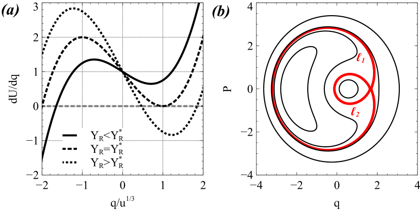
Figure 38: (a) Profiles of $dU/dq=\tilde{q}^{3}/2-(3/2)\tilde{q}(Y_{R}/Y_{R}^{*})+1$ for different $Y_{R}$; $Y_{R}^{*}=(3/2)u^{2/3}$ and $\tilde{q}=q/u^{1/3}$. (b) Phase portraits of Hamiltonian (71) with $u=2$ for $Y_{R}>Y_{R}^{*}$. Bold red curve shows the separatrices $\ell_{1,2}$.

Figure 12 shows the relation between phase portraits in Fig. 38(b) and Fig. 7(b). Hamiltonian ${\cal H}_{\zeta}$ from Eq. (6) describes the charged particle motion from the domain $G_{1}$ to the domain $G_{2}$, and this motion may include a temporary particle trapping into the domain $G_{0}$. The trapping probability is typically quite small and most of particles will move from $G_{1}$ to $G_{2}$ via a single resonance $\dot{\zeta}\propto I-I_{R}=0$ crossing. However, if initial particle $I_{x}$ ($I$) is small, we should consider Hamiltonian ${\cal L}$ to describe particle motion. Small $I$ means small $Y$, and thus small area $I_{P}$ in the phase portrait of Hamiltonian ${\cal L}$. Thus, particles will small $I$ (small $I_{P}$) appear within the $G_{0}$ domain in the phase portrait, whereas particles with large $I_{P}$ will move along the orbits outside the $\ell_{1}$ separatrix (see Fig. 38(b)), within the $G_{1}$ domain. This predicts that most of particles with small $I$ experience the phase trapping.

Particles having $I$ sufficiently large to start motion in $G_{1}$ domain, but sufficiently small to be described by ${\cal L}$ Hamiltonian, can experience the phase trapping (transition from $G_{1}$ to $G_{0}$) or phase bunching (scattering; transition from $G_{1}$ to $G_{2}$). The latter transition happens when crossing the separatrix $\ell_{1}$, which will result in $I_{P}$ jump, $\Delta I_{P}=\Delta{\cal S}/2\pi$, where $\Delta{\cal S}$ is the difference of areas of $G_{1}$ and $G_{2}$ domains. This $I_{P}$ jump is directly related to the jump of $I$ (and $I_{x}$)

$$\Delta I_{x}=\Delta I=\frac{{mc^{2}\Delta{\cal S}}}{{2\pi\Omega_{0}}}\left({\frac{{eA_{w}}}{{m_{e}c^{2}}}}\right)^{2/3}$$ (72)

This scaling $\Delta I_{x}\propto A_{w}^{2/3}\propto{\cal B}_{w}^{2/3}$ differs from the phase bunching scaling $\Delta I_{x}\propto{\cal B}_{w}^{1/2}$ derived in Section 3. Therefore, two main features of small $I$ (small pitch-angle) systems are: (a) a large probability of trapping, when electrons are already within the trapping region when the separatrix appears, (b) a different scaling of momentum (energy) jump due to phase bunching.

Appendix C

In this Appendix we describe the limit of a small area ${\cal S}$ system, i.e., such systems where parameter $a=|{\rm B}/{\rm A}|$ from Hamiltonian (6) is about one. To make nonlinear resonant interaction possible, we assume that $|{\rm A}|$ becomes smaller than $|{\rm B}|$, but to keep ${\cal S}$ small the inequality $a>1$ holds only within a short range of magnetic latitudes, i.e., over a short range of resonant energies, $\gamma_{R}$. Then, the $\zeta$ range of the area filled with closed trajectories (where $\zeta\in[\zeta_{-},\zeta_{+}]$ in Fig. 7(b), $\zeta_{-}$ is the saddle point, and $\zeta_{+}$ is the coordinate of separatrix crossing $P_{\zeta}=0$, right from the $\zeta_{-}$) is small and Hamiltonian (6) can be expanded as:

$${\cal H}_{\zeta}=\frac{1}{2M}P_{\zeta}^{2}+{\rm B}\cdot\left({\frac{1}{a}\zeta+\cos\zeta}\right)\approx\frac{1}{2M}P_{\zeta}^{2}+{\rm B}\cdot\left({\left({\frac{1}{a}-1}\right)\zeta+\frac{1}{6}\zeta^{3}}\right)$$ (73)

where $1/a$ slowly changes along the trajectory from $>1$ (no closed trajectories in the phase portrait) to $\min 1/a<1$ (maximum area filled by closed trajectories), and then to $>1$ again. This expansion is around $\zeta=pi/2$, because $\zeta_{\pm}\to\pi/2$ with $a\to 1$ accordingly to equation $\sin\zeta=1/a$. Figure 39(a) shows the phase portrait of Hamiltonian (73) for such $1/a<1$. There are two small system parameters: ${\rm B}\propto{\cal D}\propto k^{-1}(\partial\ln\Omega_{0}/\partial)\ll 1$ and ${\rm A}\propto{\cal B}_{w}/B_{0}\ll 1$. When these two parameters are of the same order of magnitude, $a=|{\rm B}/{\rm A}|\sim 1$. In this Appendix we introduce $\varepsilon\ll 1$ such that ${\rm B}\propto\varepsilon$ and ${\rm A}\propto\varepsilon$, so that $\tilde{\rm A}={\rm A}/\varepsilon$ is of the order of one. To model the system evolution we can write $1/a=1-\delta_{0}+(\varepsilon t)^{2}$ where the small parameter $\delta_{0}>0$ determines how far $1/a$ is from $1$ and $(\varepsilon t)^{2}$ models the slow evolution of $1/a$ along the trajectory (i.e., we change here the slow coordinate $s$ to a slow time):

$${\cal H}_{\zeta}\approx\frac{1}{2M}P_{\zeta}^{2}-\varepsilon\tilde{{\rm A}}\cdot\left({\left({\delta_{0}-\left({\varepsilon t}\right)^{2}}\right)\zeta-\frac{1}{6}\zeta^{3}}\right)$$ (74)

and $M$, $\tilde{\rm A}$ can be considered as constant along a short interval of $\varepsilon t\in[-\sqrt{\delta_{0}},\sqrt{\delta_{0}}]$. The equation for ${\cal S}$ for Hamiltonian (6) can be written as

$${\cal S} = \sqrt{8\varepsilon\tilde{\rm A}M}\int\limits_{\zeta_{+}}^{\zeta-}{\left({\left({\delta_{0}-\left({\varepsilon t}\right)^{2}}\right)\left({\zeta-\zeta_{+}}\right)-\frac{{\zeta^{3}-\zeta_{+}^{3}}}{6}}\right)^{1/2}d}\zeta$$ (75)

$$= \sqrt{8\varepsilon\tilde{\rm A}M}\delta_{0}^{5/4}\left({1-\frac{{t^{2}}}{{t_{0}^{2}}}}\right)^{5/4}\int\limits_{\bar{\zeta}_{+}}^{\bar{\zeta}-}{\left({\left({\bar{\zeta}-\bar{\zeta}_{+}}\right)-\frac{{\bar{\zeta}^{3}-\bar{\zeta}_{+}^{3}}}{6}}\right)^{1/2}d}\bar{\zeta}$$

$$= \sqrt{8\varepsilon\tilde{\rm A}M}\delta_{0}^{5/4}\left({1-\left({t/t_{0}}\right)^{2}}\right)^{5/4}\cdot\frac{{12\cdot 2^{3/4}}}{5}$$

where $\bar{\zeta}_{+}=-\sqrt{2}$, $\bar{\zeta}_{-}=\sqrt{8}$, $t_{0}=\sqrt{\delta_{0}}/\varepsilon$ and $t/t_{0}$ is equivalent to $\gamma_{R}$, the energy at resonance, because different slow time values imply here different values of slow $s$, i.e., different values of the resonant $s_{R}$ related to $\gamma_{R}$ through Eq. (4). Equation (75) demonstrates that the $\delta_{0}$ parameter controls the magnitude of ${\cal S}$, and effects of nonlinear interactions should disappear when $\delta_{0}\to 0$. In the nonlinear regime, there are well separated populations of trapped particles (a small number of particles gaining a large energy) and phase bunched particles (a large number of particles losing energy). In contrast, in the diffusive regime the numbers of particles gaining and losing energy are (approximately) equal. Therefore, there is a threshold $\delta_{0}$ value (or ${\cal S}$ value) such that for $\delta_{0}$ below this threshold, we cannot separate trapping and nonlinear scattering. Let us derive an expression for this threshold $\delta_{0}$ (or ${\cal S}$) value.

Hamiltonian equations for Hamiltonian (74) can be combined to get the second order equation for $\zeta$:

$$\frac{{d^{2}\zeta}}{{d\tilde{t}^{2}}}=\varepsilon\cdot\left({\delta_{0}-\left({\varepsilon\tilde{t}}\right)^{2}-\frac{1}{2}\zeta^{2}}\right)$$ (76)

where $\tilde{t}=t\sqrt{\tilde{\rm A}M}$ and $\tilde{\rm A}$, $M$ are constants of the order of one (not dependent on $\varepsilon$). Equation (76) can be rewritten in normalized variables $\tau=\tilde{t}\varepsilon^{1/2}\delta_{0}^{1/4}$, $\xi=\zeta/\sqrt{\delta_{0}}$

$$\frac{{d^{2}\xi}}{{d\tau^{2}}}=\left({1-\frac{\varepsilon}{{\delta_{0}^{3/2}}}\tau^{2}}\right)-\frac{1}{2}\xi^{2}$$ (77)

Equation (77) shows that for $\delta_{0}=\varepsilon^{2/3}$ there is no separation of time-scales, i.e. the equation describing electron motion around the resonance does not contain a slow time. Thus, both trapped and nonlinearly scattered particles should stay in the resonance approximately the same time, and there is no separation between these two types of trajectories. Figure 39(b) confirms this conclusion: we solve equation Eq. (77) with $\delta_{0}=\varepsilon^{2/3}$ for set of trajectories and plot these trajectories in the phase plane $(\xi,d\xi/d\tau)$. There are still some trajectories similar to trapped trajectories of the original system, but particles on these trajectories do not fulfil a single oscillation across the resonance $d\xi/d\tau=0$, i.e., we cannot separate particles on trapped and scattered trajectories.

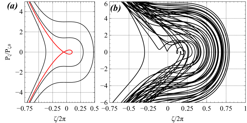
Figure 39: The phase portrait of Hamiltonian (73) for $r/u$ around $1$ (a). Set of trajectories obtained by numerical integration of Eq. (77) with $\delta_{0}=\varepsilon^{2/3}$.

The parameter $\delta_{0}$ controls the effective range of energy change due to trapping, and should be related to the number of complete rotations around the resonance of trapped particles, $N_{trap}$. Thus, we can derive the $\delta_{0}(N_{trap})$ dependence. We define $N_{trap}$ as the maximum number of periods of a trapped particle’s rotation in the phase space (see phase portrait in Fig. 39(b)). This parameter is quite universal: it can be determined for any particular wave-field model (see, e.g., Zhang, Thorne, Artemyev, Mourenas, Angelopoulos, Bortnik, Kletzing, Kurth & Hospodarsky [2018] for a discussion of $N_{trap}$ values typical for whistler-mode waves observed in the Earth’s radiation belts). The trapped period for Hamiltonian (74) can be written as

$$T_{trap}\left({\varepsilon t}\right)=2\int\limits_{\zeta_{-}}^{\zeta_{{}_{+}}}{\frac{{d\zeta}}{{\dot{\zeta}}}}=\frac{C}{{\varepsilon^{1/2}\left({\delta_{0}-\varepsilon^{2}t^{2}}\right)^{1/4}}}$$ (78)

where constant $C\sim O(1)$ is determined by the distance from the separatrix in the phase portrait. The maximum time of trapped particle motion is of the order of $\sim 2\delta_{0}^{1/2}/\varepsilon$. Therefore we can write for $N_{trap}$

$$N_{trap}=\frac{2}{\varepsilon}\int\limits_{0}^{\sqrt{\delta_{0}}}{\frac{{d\varepsilon t}}{{T_{trap}\left({\varepsilon t}\right)}}}=\frac{{\delta_{0}^{3/4}}}{{\sqrt{\varepsilon}}}\tilde{C}\sim\varepsilon^{3\kappa/5-1/2}$$ (79)

where constant $\tilde{C}\sim O(1)$. Equation (79) shows that $N_{trap}\sim\varepsilon^{3\kappa/5-1/2}$. For the threshold value $\kappa=5/6$, we get $N_{trap}\sim O(1)$, i.e., for $\kappa=5/6$ ($\delta_{0}\sim\varepsilon^{2/3}$) the number of trapping periods does not depend on $\varepsilon$ and there is no separation between trapped and scattered particles anymore.

Appendix D

In this Appendix we consider an important property of resonant systems described by the Hamiltonian ${\cal H}_{I}={\cal H}_{0}\left(I,s,p\right)+\varepsilon{\cal H}_{1}\left(I,\zeta,s,p\right)$ with $\varepsilon=const\ll 1$: the gain of phase $\zeta$ between two successive resonances is a random value. The rigorous proof of this property can be found in [Gao et al., 2023], whereas a simplified version of this proof is provided below [this derivation is somewhat similar to the derivation provided in Neishtadt & Vasiliev, 2005]. Examples with ${\cal H}_{0}=-\omega I+\gamma(s,p,I)$, $\varepsilon{\cal H}_{1}=-eU_{w}(s,I)\cos\zeta$, and $\varepsilon\sim{\cal B}_{w}/B_{0}$ are provided by Eq. (LABEL:eq:hamiltonian_const), but within this Appendix we do not use explicit forms for $H_{0}$, $H_{1}$. In this Hamiltonian $(s,\varepsilon^{-1}p)$, $(\zeta,I)$ are pairs of conjugate variables (hence $(\zeta,I)$ are fast variables, $(q,p)$ are slow variables), and ${\cal H}_{1}$ is periodic in $\zeta$. Momentum $I$ is an adiabatic invariant: $\dot{I}=-\varepsilon\partial{\cal H}_{1}/\partial\zeta$, and $I$ is constant in the averaged over $\zeta$ system. There is no explicit dependence on time, and thus ${\cal H}_{I}=h={\rm const}$. The resonance condition is determined by the equation $\partial{\cal H}_{0}/\partial I=0$. Solving this equation for $I$ gives the equation $I=I_{R}(s,p)$ of the surface of resonance. Denote $\Lambda(s,p)={\cal H}_{0}(I_{R}(s,p),s,p)$. The Hamiltonian can be expanded around the resonance surface similarly to Eq. (6). For variables $\zeta$ and $P_{\zeta}=I-I_{R}$ we get Hamiltonian

$${\cal H}_{\zeta}=\frac{1}{{2M}}P_{\zeta}^{2}+{\rm A}\zeta+{\cal H}_{1}$$

where

$$M^{-1}=\left.{\frac{{\partial^{2}{\cal H}_{0}}}{{\partial I^{2}}}}\right|_{I=I_{R}}\approx{\rm const},\quad{\rm A}=\left\{{\Lambda,I_{R}}\right\}\approx{\rm const}.$$

We assume that the phase portrait of the Hamiltonian ${\cal H}_{\zeta}$ looks like one shown in Fig. 40 (we put $I$ instead of $P_{\zeta}$ onto the vertical axis there).

We introduce the improved adiabatic invariant $J$ with the variable transformation $(I,\zeta,p,s)\mapsto(J,\theta,P,Q)$ such that the new Hamiltonian is ${\cal H}={\cal H}_{0}(J,P,Q)+\varepsilon\bar{\cal H}_{1}(J,P,Q)$, where $\bar{\cal H}_{1}$ is the average of ${\cal H}_{1}$ over $\zeta$ (in the leading approximation).

Far from the resonance $\theta$ changes with the frequency

$$\dot{\theta}=\frac{{\partial{\cal H}_{0}}}{{\partial J}}+\varepsilon\frac{{\partial\bar{\cal H}_{1}}}{{\partial J}}$$ (80)

with $J={\rm const}$, and

$$\dot{Q}=\varepsilon\frac{{\partial{\cal H}_{0}}}{{\partial P}}+\varepsilon^{2}\frac{{\partial\bar{\cal H}_{1}}}{{\partial P}},\quad\dot{P}=-\varepsilon\frac{{\partial{\cal H}_{0}}}{{\partial Q}}-\varepsilon^{2}\frac{{\partial\bar{\cal H}_{1}}}{{\partial Q}}$$ (81)

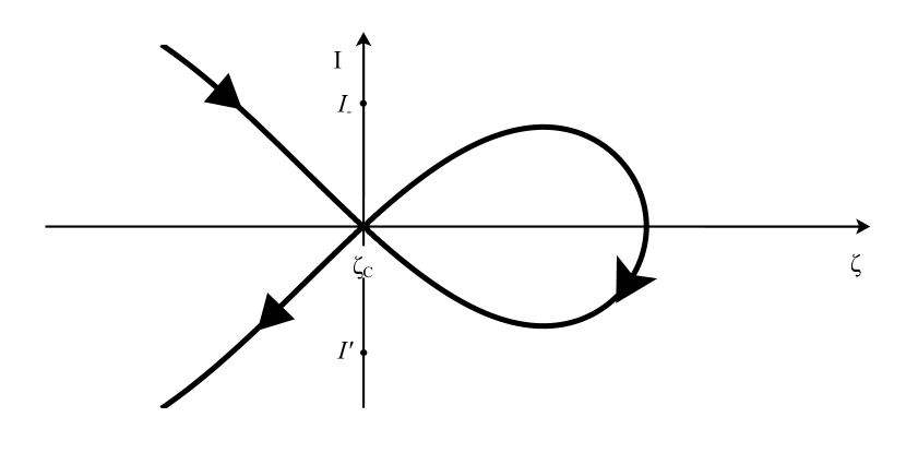
Figure 40: Schematic of phase portrait.

We introduce $\omega_{0}(J,P,Q)=\partial{\cal H}_{0}/\partial J$, $\omega_{1}(J,P,Q)=\partial\bar{H}_{1}/\partial J$, and consider a large number $N\gg 1$ of rounds of $\zeta$ from $t=t_{0}$ (when phase point is far from the resonance and moves towards the resonance) to $t=t_{N}$; the last round is sufficiently far from the resonance and $\theta\approx\zeta$ in the leading approximation. The last round ends at at $\zeta=\zeta_{cN}=\zeta_{c}\ {\rm mod}\ 2\pi$; (see Fig. 40 for the definition of $\zeta_{c}$). Then

$$\zeta_{c}=\zeta_{0}+\int\limits_{t_{0}}^{t_{N}}{\left({\omega_{0}+\varepsilon\omega_{1}}\right)dt}\quad{\rm mod}\ 2\pi.$$ (82)

We introduce $t_{*}$ as the time of crossing the resonance, i.e. $\omega_{0}(J,P,Q)|_{t=t_{*}}=0$, and rewrite Eq. (82):

$$\zeta_{c}=\zeta_{0}+\int\limits_{t_{0}}^{t_{*}}{\left({\omega_{0}+\varepsilon\omega_{1}}\right)dt}-\int\limits_{t_{N}}^{t_{*}}{\left({\omega_{0}+\varepsilon\omega_{1}}\right)dt}\quad{\rm mod}\ 2\pi$$ (83)

Because $t_{*}-t_{N}\ll 1/\varepsilon$ we can use $\dot{Q}=\varepsilon\partial{\cal H}_{0}/\partial P$, $\dot{P}=-\varepsilon\partial{\cal H}_{0}/\partial P$ and $Q\approx q$, $P\approx p$ in the last integral in Eq. (83). We also assume that $\zeta_{c}\approx\zeta_{c*}=\zeta_{c}|_{t=t_{*}}$. Thus, we can replace $\zeta_{c}$ with $\zeta_{c*}$ in (83).

To describe system dynamics for $t\in[t_{N},t_{*}]$ we use the expansion of the Hamiltonian around the resonance: $H=\Lambda+\Upsilon$ and

$$\Upsilon=\frac{1}{2M}\left({I-I_{R}}\right)^{2}+\varepsilon{\cal H}_{1}.\;\;$$ (84)

The Hamiltonian in new variables $(J,\theta,P,Q)$ can be expanded as

$${\cal H}=\Lambda+\frac{1}{2M}\left({J-I_{R}}\right)^{2}+\varepsilon\bar{H}_{1}$$ (85)

We introduce ${\epsilon}=(J-I_{R})^{2}/2M$ and write

$$\dot{{\epsilon}} = -\varepsilon M^{-1}\left({J-I_{R}}\right){\rm A},\quad{\rm A}=\left\{{\Lambda,I_{R}}\right\}\approx{\rm const}$$

$$\omega_{0} = \frac{{\partial{\cal H}}}{{\partial J}}=M^{-1}\left({J-I_{R}}\right)$$ (86)

Using $dt=d{\epsilon}/(d{\epsilon}/dt)$ we rewrite integral

$$\int\limits_{t_{N}}^{t_{*}}{\left({\omega_{0}+\varepsilon\omega_{1}}\right)dt}\approx-\frac{1}{\varepsilon}\int\limits_{{\epsilon}_{N}}^{0}{\frac{{\omega_{0}d{\epsilon}}}{{g\left({J-I_{R}}\right){\rm A}}}}=-\frac{1}{\varepsilon}\int\limits_{{\epsilon}_{N}}^{0}{\frac{{d{\epsilon}}}{{\rm A}}}=\frac{{{\epsilon}_{N}}}{{\varepsilon{\rm A}}}$$ (87)

where ${\epsilon}_{N}$ is the value ${\epsilon}$ along the trajectory at $t=t_{N}$, and we omit $\varepsilon\omega_{1}$ because $t_{*}-t_{N}\ll 1/\varepsilon$. Using ${\epsilon}+\varepsilon\bar{\cal H}_{1}=\Upsilon$, we write

$${\epsilon}_{N}=\Upsilon_{N}-\varepsilon\bar{\cal H}_{1}\approx\Upsilon_{N}-\varepsilon\bar{\cal H}_{1*}$$ (88)

where $\Upsilon_{N}$ is the value $\Upsilon$ along the trajectory at $t=t_{N}$, and $\bar{\cal H}_{1*}$ is the resonant value of $\bar{\cal H}_{1}$. Substituting Eqs. (87, 88) to Eq. (83), we obtain

$$\zeta_{c*}=\zeta_{0}+\int\limits_{t_{0}}^{t_{*}}{\left({\omega_{0}+\varepsilon\omega_{1}}\right)dt}-\frac{{\Upsilon_{N}-\varepsilon\bar{\cal H}_{1*}}}{{\varepsilon{\rm A}}}\quad{\rm mod}\ 2\pi$$ (89)

or

$$\frac{{\Upsilon_{N}}}{{2\pi\varepsilon{\rm A}}}=\frac{{\bar{\cal H}_{1*}}}{{2\pi{\rm A}}}+\frac{1}{{2\pi}}\left({\zeta_{0}-\zeta_{c*}+\int\limits_{t_{0}}^{t_{*}}{\left({\omega_{0}+\varepsilon\omega_{1}}\right)dt}}\right)\,\,\,\bmod 1$$ (90)

We define $\Upsilon_{last}$ as the value of $\Upsilon$ along the trajectory at the last crossing of the line $\zeta=\zeta_{c}$ before crossing the resonance. Thus, $\Upsilon_{last}=\Upsilon_{N}\ {\rm mod}\ 2\pi\varepsilon{\rm A}$, because the change of $\Upsilon$ for one round of $\zeta$ equals $2\pi\varepsilon{\rm A}$. We introduce $\xi=(\Upsilon_{last}-\varepsilon{\cal H}_{1c*})/(2\pi\varepsilon{\rm A})$, where ${\cal H}_{1c*}$ is value of ${\cal H}_{1}$ at $\zeta=\zeta_{c}$, $t=t_{*}$ and write

$$\xi={\mathop{\rm Frac}\nolimits}\left(\frac{{\bar{\cal H}_{1*}-{\cal H}_{1c*}}}{{2\pi{\rm A}}}+\frac{{\zeta_{0}-\zeta_{c*}}}{{2\pi}}+\frac{1}{2\pi\varepsilon}\int\limits_{\tau_{0}}^{\tau_{*}}\left(\omega_{0}+\varepsilon\omega_{1}\right)d\tau\right)$$ (91)

Here $\tau=\varepsilon t$, $\tau_{*}=\varepsilon t_{*}$. Note that $\xi$ can be written as

$$\xi=\frac{{\Upsilon_{last}-\varepsilon H_{1c*}}}{{2\pi\varepsilon r}}=\frac{{\Upsilon_{last}+\varepsilon{\rm A}\zeta_{c*}-\left({\varepsilon H_{1c*}+\varepsilon{\rm A}\zeta_{c*}}\right)}}{{2\pi\varepsilon{\rm A}}}=\frac{{\cal E}_{last}-{\cal E}_{c*}}{2\pi\varepsilon{\rm A}}$$ (92)

where

$${\cal E}=\frac{1}{2M}\left({I-I_{R}}\right)^{2}+\varepsilon{\rm A}\zeta+\varepsilon{\cal H}_{1},$$ (93)

and ${\cal E}_{c*}$ is the value of ${\cal E}$ at $\zeta=\zeta_{c}$, $t=t_{*}$, ${\cal E}_{last}$ is the value of ${\cal E}$ at the last crossing of the line $\zeta=\zeta_{c}$ before crossing the resonance.

Let us use Eq. (91) to consider two successive crossings of the same resonance in the same direction. During the period of a slow motion a particle crosses the same resonance twice in opposite directions. We consider crossing the resonance in direction from positive to negative value of frequency, as in Fig.40, assuming that for crossing in the opposite direction we have $H_{1}\equiv 0$. Then there is only one resonant interaction for one period of slow motion, i.e. two successive resonance crossings are separated by one slow period. Far from the resonance the improved adiabatic invariant $J$ can be considered as a constant. Denote $\tau_{-}$ and $\tau_{+}$ slow time moments of the resonance crossings ($\tau=\varepsilon t$). Let $\xi_{\pm}$ be values of the variable $\xi$ corresponding to these two crossings. We are looking for a relation between $\xi_{+}$ and $\xi_{-}$. Due to periodicity of the slow motion, values of $\zeta_{c*}$, ${\cal H}_{1c*}$, $\bar{\cal H}_{1*}$, ${\rm A}$ are the same at $\tau=\tau_{+}$ and $\tau=\tau_{-}$.

We consider value $\xi_{-}$ for the first of the resonance crossings, and the corresponding value ${\cal E}={\cal E}_{last-}$. At $\tau=\tau_{-}$ the phase point is on the line $\zeta=\zeta_{c*}$ with $I>I_{R}$ at the position indicated by the symbol $I_{-}$ in Fig. 40. We assume that this phase point crosses the resonance without trapping. Thus, at some $\tau=\tau^{\prime}$ it arrives again to the line $\zeta=\zeta_{c}=\zeta_{c*}^{\prime}$ with the value ${\cal E}={\cal E}^{\prime}$ and $I<I_{R}$. The phase point position is indicated by the symbol $I^{\prime}$ in Fig. 40. We denote $\xi^{\prime}=({{\cal E}^{\prime}-{\cal E}_{c*}})/({2\pi\varepsilon{\rm A}})$.

At some moment of the slow time $\tau_{0}\in(\tau_{-},\tau_{+})$ the phase point is far from the resonance and has $\zeta=\zeta_{0}$. Then Eq. (91) gives

$$\xi_{+}={\mathop{\rm Frac}\nolimits}\left(\frac{{\bar{\cal H}_{1*}-{\cal H}_{1c*}}}{{2\pi{\rm A}}}+\frac{{\zeta_{0}-\zeta_{c*}}}{{2\pi}}+\frac{1}{2\pi\varepsilon}\int\limits_{\tau_{0}}^{\tau_{+}}\left(\omega_{0}+\varepsilon\omega_{1}\right)d\tau\right)$$ (94)

Similarly, considering the backward motion on the time interval from $\tau_{0}$ to $\tau^{\prime}$ we get

$$\xi^{\prime}={\mathop{\rm Frac}\nolimits}\left({\frac{{\bar{\cal H}_{1*}-{\cal H}_{1c*}}}{{2\pi{\rm A}}}+\frac{{\zeta_{0}-\zeta_{c*}}}{{2\pi}}-\frac{1}{2\pi\varepsilon}\int\limits_{\tau^{\prime}}^{\tau_{0}}{{{\left({\omega_{0}+\varepsilon\omega_{1}}\right)}}d\tau}}\right)$$ (95)

In this expression we can replace in the leading approximation $\xi^{\prime}$ with $\xi_{-}$ and $\tau^{\prime}$ with $\tau_{-}$ (note that

$$\frac{1}{2\pi\varepsilon}\int\limits_{\tau_{-}}^{\tau^{\prime}}\left({\omega_{0}+\varepsilon\omega_{1}}\right)d\tau$$

is small, because $\omega_{0}$ vanishes on the resonant surface). Thus for the value $\Delta\xi=\xi_{+}-\xi_{-}$ we get

$$\Delta\xi=\xi_{+}-\xi_{-}=\frac{1}{2\pi\varepsilon}\int\limits_{\tau_{-}}^{\tau_{+}}{{\left({\omega_{0}+\varepsilon\omega_{1}}\right)}}{d\tau}\ {\rm mod}\ 1\phantom{***}$$ (96)

and this describes the phase $\zeta$ gain between two resonance crossings (between moments $\tau_{-}$ and $\tau_{+}$) normalized on $2\pi$. In the main text $\bar{\cal H}_{1}=0$ and thus $\omega_{1}=\partial\bar{H}_{1}/\partial J=0$.

Appendix E

In this Appendix, we demonstrate the applicability of the mapping technique for two types of events observed in the outer radiation belts. Both events are associated with energetic electron precipitations via scattering by whistler-mode waves. Such scattering corresponds to a decrease of the electron equatorial pitch-angle $\alpha_{eq}$ and a change of electron energy. Field-aligned chorus waves interact with electrons through the first cyclotron resonance. The nonlinear regime of this resonant interaction includes phase trapping (with $\alpha_{eq}$ and energy increase, see, e.g., Omura et al. [2015]) and phase bunching (with $\alpha_{eq}$ and energy decrease, see, e.g., Albert [2000]; Vainchtein et al. [2018]). The competition between phase trapping and phase bunching Istomin et al. [1973]; Solovev & Shkliar [1986]; Shklyar [2011]; Artemyev, Neishtadt, Vasiliev & Mourenas [2016] controls the net electron transport into the loss-cone, but all precipitating electrons lose energy, because precipitation is provided only by phase bunching. Thus, both linear and non-linear electron interaction with chorus via the cyclotron resonance is associated with electron deceleration. Such effective scattering and deceleration of electrons by field-aligned waves is modeled with the mapping technique in Subsection Appendix E.2.

Although field-aligned chorus waves are the most intense whistler-mode wave population in the radiation belt Li, Bortnik, Thorne & Angelopoulos [2011]; Agapitov et al. [2013], there is also a significant population of very oblique whistler-mode waves (almost electrostatic mode, see Artemyev, Agapitov, Mourenas, Krasnoselskikh, Shastun & Mozer [2016]) propagating near the resonance cone angle Agapitov et al. [2013, 2018]; Li, Santolik, Bortnik, Thorne, Kletzing, Kurth & Hospodarsky [2016]. These oblique waves can interact resonantly with electrons through Landau resonance [e.g., Shklyar & Matsumoto, 2009; Nunn & Omura, 2015] and can accelerate electrons efficiently via phase trapping Artemyev et al. [2012]; Agapitov et al. [2014]; Hsieh & Omura [2017a]; Hsieh et al. [2020]. The corresponding Landau resonant energies are much lower than cyclotron resonant energies with quasi-parallel waves, allowing very oblique waves to resonate with $100$ eV - $10$ keV electrons Mourenas, Artemyev, Agapitov & Krasnoselskikh [2014]; Artemyev, Agapitov, Mourenas, Krasnoselskikh & Mozer [2015]; Artemyev, Agapitov, Mourenas, Krasnoselskikh, Shastun & Mozer [2016] which can almost never be scattered by field-aligned lower-band chorus waves Li et al. [2010]. Moreover, in contrast to the cyclotron resonance associated with an energy decrease of precipitating electrons, the Landau resonant trapping is associated with energy increase (see Figs. 6 and 20). Thus, precipitating electrons (those with decreasing $\alpha_{eq}$) are simultaneously accelerated, corresponding to an increase of low-$\alpha_{eq}$ energetic electron flux Agapitov et al. [2015b]. Since very oblique whistler-mode waves can be quite intense Cully, Bonnell & Ergun [2008]; Cattell et al. [2008]; Wilson et al. [2011]; Agapitov et al. [2014], these waves may in principle interact nonlinearly with electrons and efficiently trap them through Landau resonance Agapitov et al. [2015b]; Mourenas et al. [2016]. Such trapping results in intense, short-lived precipitation of $\lesssim 200$ keV electrons Zhang, Artemyev, Angelopoulos, Tsai, Wilkins, Kasahara, Mourenas, Yokota, Keika, Hori, Miyoshi, Shinohara & Matsuoka [2022]; Artemyev, Zhang, Zou, Mourenas, Angelopoulos, Vainchtein, Tsai & Wilkins [2022]. An important feature of this precipitation mechanism is the loss-cone overfilling, when precipitating fluxes at low altitudes appear to be larger than quasi-trapped fluxes just outside of the loss-cone Zhang, Artemyev, Angelopoulos, Tsai, Wilkins, Kasahara, Mourenas, Yokota, Keika, Hori, Miyoshi, Shinohara & Matsuoka [2022]. In Subsection Appendix E.1 we provide a simulation of this effect using the mapping technique.

The loss-cone size $\alpha_{LC}$ (the maximum pitch-angle range of precipitating electrons) in the outer radiation belt around the magnetic equator is only a few degrees, which makes it challenging for near-equatorial spacecraft to directly measure such electron losses Kasahara, Miyoshi, Yokota, Kasahara, Matsuda, Kumamoto, Matsuoka, Kazama, Frey, Angelopoulos, Kurita, Keika, Seki & Shinohara [2018]. Spacecraft at low altitudes (where magnetic field is large and $\alpha_{LC}$ reaches $60-70^{\circ}$), however, can easily measure electron fluxes within the loss cone. Conjugate spacecraft measurements of near-equatorial waves responsible for electron scattering into the loss cone and low-altitude electron fluxes within it, are optimal for testing theoretical models of electron scattering and precipitation by waves. Li, Ni, Thorne, Bortnik, Green, Kletzing, Kurth & Hospodarsky [2013]. Thus, we use such a combination of observations from the equatorial THEMIS-E spacecraft Angelopoulos [2008] and the low-altitude ($\sim 400-450$ km) ELFIN spacecraft Angelopoulos et al. [2020].

The two identical CubeSats of the Electron Losses and Fields Investigation (ELFIN) mission were launched on September 15th, 2018, with onboard energetic particle detectors of ions (EPD-I) and electrons (EPD-E) Angelopoulos et al. [2020]. Electrons are measured in an energy range from 50 keV to $\sim 6$ MeV with an energy resolution ($\Delta E/E$) less than 40 % and a time resolution ($T_{spin}$) of $\sim 2.85$ s Angelopoulos et al. [2023]; Tsai & et al. [2024]. The high resolution of the pitch-angle of the EPD-E ($\Delta\alpha\simeq 22.5^{\circ}$) enables it to distinguish trapped electrons (outside the local bounce loss cone) from precipitation electrons (within the local bounce loss cone) [Zhang, Angelopoulos, Mourenas, Artemyev, Tsai & Wilkins, 2022; Angelopoulos et al., 2023, see details]. The ratio of the precipitating electron flux and the trapped electron flux, $j_{prec}/j_{trap}$, indicates the efficiency of equatorial electron scattering by waves Mourenas et al. [2021]; Zhang, Artemyev, Angelopoulos, Tsai, Wilkins, Kasahara, Mourenas, Yokota, Keika, Hori, Miyoshi, Shinohara & Matsuoka [2022]; Shen et al. [2022]; Capannolo et al. [2023] or of the magnetic field line curvature process Wilkins et al. [2023]; Zou et al. [2024]. In this Appendix, we consider two ELFIN events with electron scattering by whistler-mode waves [additional examples are provided in Chen et al., 2022; Tsai et al., 2022; Zhang, Angelopoulos, Artemyev, Mourenas, Agapitov, Tsai & Wilkins, 2023; Gan et al., 2023; Kang et al., 2024].

Appendix E.1: Nonlinear Landau resonance: loss-cone overfilling effect

Figure 41(a) is an overview of THEMIS E measurements on 2021-01-01 from 22:20 to 23:30 UT in the dayside inner magnetosphere, when the spacecraft moved outward from $L\sim 7$ to $L\sim 9$ ($L$ is evaluated with the Tsyganenko [1989] magnetic field model). There is strong whistler-mode wave activity within the frequency range $f/f_{ce}\in[0.2,0.4]$, where the electron cyclotron frequency $f_{ce}$ is calculated from in-situ measurements from the fluxgate magnetometer Auster et al. [2008] and the wave spectrum is obtained from the search coil Le Contel et al. [2008]; Cully, Ergun, Stevens, Nammari & Westfall [2008]. Using plasma density estimates from the spacecraft potential Nishimura et al. [2013], we can estimate the plasma frequency to electron gyrofrequency ratio, $f_{pe}/f_{ce}\sim 3$. Figure Figure 41(b) shows several whistler-mode wave packets with a large parallel electric field component, suggesting the presence of very oblique whistler-mode waves Artemyev, Agapitov, Mourenas, Krasnoselskikh, Shastun & Mozer [2016]. Using $f_{pe}/f_{ce}$ and 3D electric fields, we estimate the wave normal angle $\theta$ for these wave-packets: $\theta\in[60,70]$ (see details of $\theta$ estimation method in Ni, Thorne, Meredith, Shprits & Horne [2011]; Agapitov et al. [2014]), with a Gendrin angle $\theta_{g}={\rm acos}(2f/f_{ce})\approx 45^{\circ}$ and a resonance cone angle $\theta_{r}={\rm acos}(f/f_{ce})\approx 69^{\circ}$. Thus, the observed waves indeed propagate obliquely with $\theta\in[\theta_{g},\theta_{r}]$, i.e., in the quasi-electrostatic mode Agapitov et al. [2013]; Li, Santolik, Bortnik, Thorne, Kletzing, Kurth & Hospodarsky [2016], and can interact with electrons through the Landau resonance Shklyar & Matsumoto [2009]; Artemyev, Agapitov, Mourenas, Krasnoselskikh, Shastun & Mozer [2016]. An interesting and important feature of the observed whistler-mode wave activity is the transient nature of wave bursts, which may be due to quasi-periodic wave generation modulated by compressional ultra-low-frequency waves Li, Thorne, Bortnik, Nishimura & Angelopoulos [2011]; Li, Bortnik, Thorne, Nishimura, Angelopoulos & Chen [2011]; Xia et al. [2016]; Zhang, Chen, Artemyev, Angelopoulos & Liu [2019]. Indeed, measurements of precipitating electrons by the Precipitating Electron and Ion Spectrometer onboard two DMSP satellites Hardy et al. [1984]; Rich et al. [1985] show clear spatially/temporally localized enhancements of $\sim 5$ keV electron precipitation, consistent with the presence of a transient (quasi-periodic) equatorial generation of very oblique whistler-mode waves [see details in Artemyev, Zhang, Zou, Mourenas, Angelopoulos, Vainchtein, Tsai & Wilkins, 2022].

There are a couple of orbits of ELFIN A and B within the same time interval and $L$-shell, MLT range [see Artemyev, Zhang, Zou, Mourenas, Angelopoulos, Vainchtein, Tsai & Wilkins, 2022, for THEMIS, DMSP, and ELFIN orbits as a function of MLT and $L$-shell]. Figure 41(c, d) shows that within the $L$-shell range corresponding to the outer radiation belt, ELFIN observed transient, strong precipitation of $<200$ keV electrons. The timescale of these precipitation bursts is about (or even less than) ELFIN’s half-spin-period, 1.5s. Therefore, we infer that these precipitation events are probably driven by electron scattering by transient whistler-mode waves which, due to their amplitude modulation by ULF waves, do not maintain the same spatial distribution at the equator over time intervals longer than $\sim 1-2$ minutes. Most of the precipitation bursts reach a ratio $\sim 1$ (and even exceed it) at energies $<200$ keV, i.e., they represent very strong precipitation with an entirely filled loss-cone, roughly corresponding to the so-called strong diffusion limit Kennel [1969] (or the loss-cone overfilling Zhang, Artemyev, Angelopoulos, Tsai, Wilkins, Kasahara, Mourenas, Yokota, Keika, Hori, Miyoshi, Shinohara & Matsuoka [2022]).

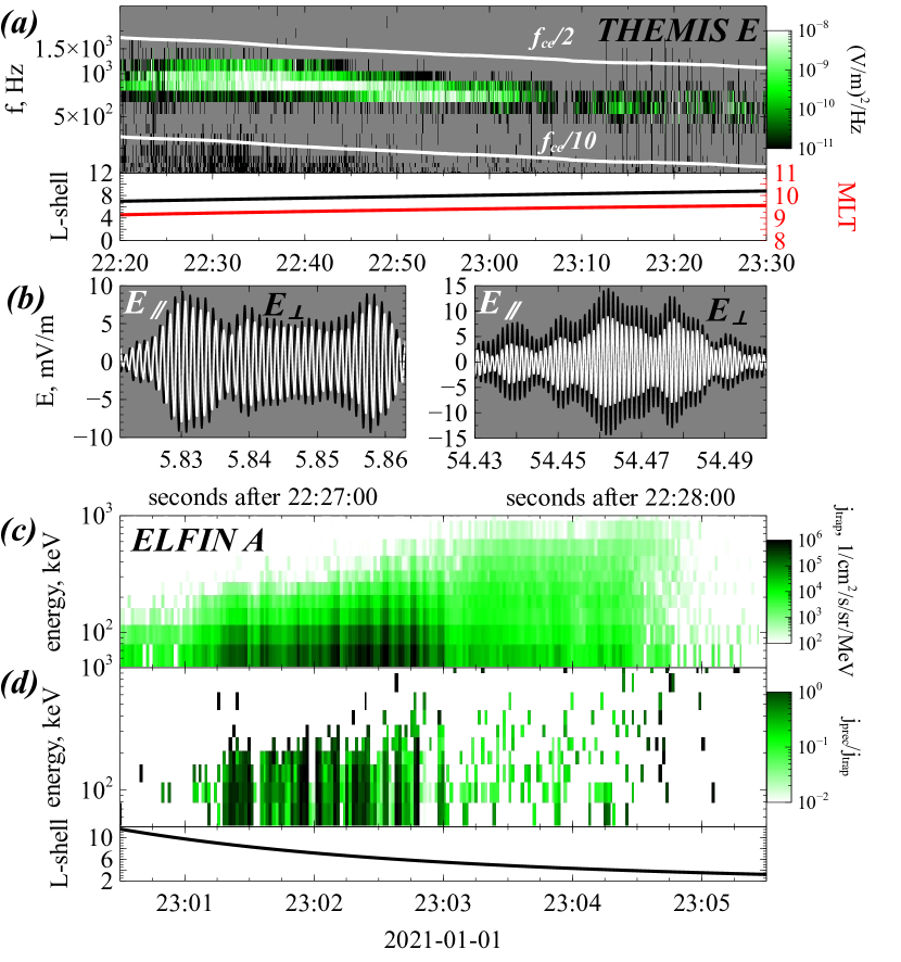
Figure 41: Overview of the event with the effect of nonlinear Landau resonance: near-equatorial THEMIS observations of whistler-mode electric field (a, b), low altitude ELFIN observations of trapped fluxes (c) and precipitating-to-trapped flux ratio (d).

To model electron precipitation by very oblique whistler-mode waves, we use the mapping technique as described by Eqs. (25). To evaluate the trapping probability, $\Pi$, and energy/pitch-angle changes due to trapping and bunching, we specify several properties of the wave model. We use a simplified model that fits the observed ${\cal B}_{w}(\lambda)$ distribution obtained from satellite statistics by Agapitov et al. [2018]:

$${\cal B}_{w}={\cal B}_{w,eq}\cdot\frac{1}{2}\left({1+\tanh\left({\lambda/\delta\lambda_{1}}\right)}\right)\cdot\exp\left({-\lambda^{2}/\delta\lambda_{2}^{2}}\right)$$ (97)

where $\delta\lambda_{1}$ determines the spatial extent of the wave generation region, and $\delta\lambda_{2}$ determines the latitude range of wave propagation before damping at middle latitudes. This model describes waves in the $\lambda>0$ hemisphere, and we assume a symmetric wave field distribution relative to the equator, i.e., ${\cal B}_{w}(\lambda)={\cal B}_{w}(-\lambda)$. Wave frequency can be assumed to be fixed along the wave propagation (or slowly varying in time, if we deal with chorus waves), whereas the wave number profile $k(\lambda)$ can be obtained from the cold plasma dispersion Stix [1962] for a given wave normal angle distribution $\theta(\lambda)$ at this particular frequency. For very oblique whistler-mode waves, we use a $\theta=\theta_{r}(\lambda)-\Delta\theta$ model, with $\theta_{r}={\rm arccos}(\omega/\Omega_{ce})$ being the resonant cone angle and $\Delta\theta=const$ the model parameter specifying the wave normal angle deviation from $\theta_{r}$. This wave normal angle model is based on previous observations of very oblique whistler-mode wave propagation around the resonance cone angle Agapitov et al. [2013]; Li, Santolik, Bortnik, Thorne, Kletzing, Kurth & Hospodarsky [2016]. The cold plasma dispersion relation does not work for $\Delta\theta\to 0$, where the thermal electron contribution to the wave dispersion properties becomes crucial Sazhin & Horne [1990]. Theoretical estimates Mourenas, Artemyev, Agapitov & Krasnoselskikh [2014]; Artemyev, Agapitov, Mourenas, Krasnoselskikh, Shastun & Mozer [2016] and spacecraft observations Ma et al. [2017] suggest that the minimum $\Delta\theta$ can be determined from the limitation of the wave refractive index $N=kc/\omega$ to values $N<N_{hot}\approx 100-300$ for typical thermal electron energies in the inner magnetosphere.

During Landau resonance ($\omega\gamma-k_{\parallel}c\sqrt{\gamma^{2}-1}\cos\alpha=0$), the electron propagates in the same direction as the wave, in contrast to cyclotron resonance characterized by opposite propagations of wave and electron. For a fixed wave frequency at Landau resonance, the resonance curve $(\omega/\Omega_{ce,eq})(\gamma^{2}-1)\sin^{2}\alpha_{eq}/2=const$ (see Fig. 6) is given by the equation of the constant magnetic moment (we use the normalized moment $I_{x}=(\omega/\Omega_{ce,eq})(\gamma^{2}-1)\sin^{2}\alpha_{eq}/2$). Combining this equation with the resonance condition, we obtain the equation for dependence of the Landau resonant energy on the magnetic latitude:

$$\gamma_{R}=\frac{1}{{\sqrt{1-\left({\omega/ck_{\parallel}}\right)^{2}}}}\sqrt{1+2I_{x}\Omega_{ce}}$$ (98)

The wave intensity increases with latitudes $dB_{w}/d\lambda>0$ around the equator Agapitov et al. [2018]; Omura et al. [2008]. This condition suggests that electrons may be trapped by waves. Being trapped at small resonant latitudes, electrons are transported by the wave to higher latitudes (with a decrease of their pitch-angle) and escape from the resonance at a latitude where $dB_{0}/d\lambda$ becomes sufficiently strong (for a precise description of the trapping and de-trapping conditions, see, Section 2.1 and e.g., Artemyev et al. [2012]; Artemyev, Vasiliev, Mourenas, Agapitov & Krasnoselskikh [2013]). Such an electron transport is associated with an energy increase, e.g., a $5$ keV equatorial electron can gain $100$ keV before reaching resonant latitudes $\sim 30^{\circ}$ and finishing within the loss-cone Artemyev, Zhang, Zou, Mourenas, Angelopoulos, Vainchtein, Tsai & Wilkins [2022]. Therefore, the trapping moves lower energy/larger pitch-angle electrons toward the larger energy/lower pitch-angle region in phase space (see schematic in Fig. 6). The Landau resonance scattering moves electrons along the same resonance curve $I_{x}=const$, but in the direction opposite to the trapping motion. Therefore, Landau resonance results in electron drifts toward smaller energy/larger pitch-angle (the phase bunching effect) and more rare jumps to larger energy/smaller pitch-angle (the phase trapping effect). Figure 42(a) shows three examples of such electron dynamics evaluated with the mapping technique (25) for typical wave characteristics (see also Fig. 20).

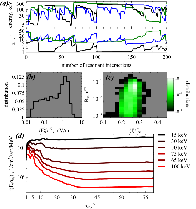
Figure 42: Panels (a) shows energy and equatorial pitch-angle for three trajectories evaluated with the mapping technique (26). Panel (b) shows the distribution of electric field amplitudes derived from the wave frequency spectra ($fff$ data) shown in Fig. 41. Panel (c) shows the distribution of wave amplitudes and frequencies for the event in Fig. 41. Wave magnetic field amplitudes are converted from the wave electric field amplitudes using cold plasma dispersion relation Tao & Bortnik [2010]. Panel (d) shows pitch-angle distributions for different energies after $\sim 10R/c\sim 2$s of interactions (sufficient to make at least one bounce period for all considered particles). The initial (equatorial) electron phase space density is obtained by fitting THEMIS E observations. We use a $K=3$ factor for this simulation, with the corresponding probability of wave-particle interactions $1/K^{2}$.

Near-equatorial spacecraft measurements of whistler-mode waves provide distributions of wave characteristics, e.g., the average wave intensity for various frequency ranges, $L$-shells, $MLT$, and $\lambda$ Meredith et al. [2001, 2012]; Agapitov et al. [2013, 2015a]. Such time-averaged intensities can be directly applied to the evaluation of quasi-linear diffusion rates [e.g., Horne, Kersten, Glauert, Meredith, Boscher, Sicard-Piet, Thorne & Li, 2013; Agapitov et al., 2018; Ma et al., 2018], but they are not suitable for the evaluation of nonlinear wave-particle interactions. Instead of time-averaged intensities, the models of nonlinear resonant wave-particle interactions require a knowledge of the distributions (occurrence rates) of intense waves that can interact with electrons nonlinearly Zhang, Thorne, Artemyev, Mourenas, Angelopoulos, Bortnik, Kletzing, Kurth & Hospodarsky [2018]; Zhang, Mourenas, Artemyev, Angelopoulos, Bortnik, Thorne, Kurth, Kletzing & Hospodarsky [2019]. Therefore, we use THEMIS E measurements during the event in Fig. 41 to obtain the distribution of wave amplitudes ${\cal E}_{w}$, as inferred from the wave frequency spectrum $\hat{E}_{w}^{2}(f)$: ${\cal E}_{w}^{2}=\int_{f_{ce}/20}^{f_{ce}/2}\hat{E}_{w}^{2}(f)df$. As shown in Figure 42(b), most waves have amplitudes $<3$ mV/m. However, $E_{w}$ here is inferred from the 1s-averaged spectrum Cully, Ergun, Stevens, Nammari & Westfall [2008] and the actual magnitude of individual wave-packets is often significantly larger (see Fig. 41). To account for such an underestimation of $E_{w}$ due to time averaging, we introduce a multiplicative factor $K$, i.e., we assume that electrons interact with waves of amplitudes $K\times E_{w}$. To keep the same average intensity as without the $K$ factor, we assume that electrons resonate with waves only a fraction ($1/K^{2}$) of the simulation time, whereas during the remaining fraction ($1-1/K^{2}$) of the time there is no resonant interaction.

The wave-particle resonant interaction is not determined solely by $E_{w}$, but also by the wave frequency, wave normal angle, and the ${\cal E}_{w}(\lambda)$ profile along the magnetic field line. The wave frequency can be determined from the wave frequency spectrum: $\langle f\rangle=\int_{f_{ce}/20}^{f_{ce}/2}f\cdot\hat{E}_{w}^{2}(f)df/{\cal E}_{w}^{2}$ (with $f_{ce}=\Omega_{0}/2\pi$ and $f=\omega/2\pi$). Figure 42(c) shows the ${\cal P}(B_{w},\langle f\rangle)$ distribution for the event in Fig. 41, with $B_{w}$ recalculated from $E_{w}$ using the cold plasma dispersion [see examples in, e.g., Ni, Thorne, Meredith, Horne & Shprits, 2011; Agapitov et al., 2014]. Using this ${\cal P}({\cal B}_{w},\langle f\rangle)$ distribution, we can rewrite the mapping in Eqs. (25) as a two-step equation. During each half of the bounce period, we generate a random number to select a $({\cal B}_{w},\langle f\rangle)$ bin from the ${\cal P}$ distribution. According to this number, we choose the wave amplitude $B_{w}$ and wave frequency $\langle f\rangle/f_{ce}$ to calculate three main characteristics of wave-particle interactions: $\Delta\gamma_{trap}$, $\Delta\gamma_{scat}$, and $\Pi$. Then, we make one iteration for energy and pitch-angle using Eq. (28). Thus, the observed distribution of wave characteristics, ${\cal P}({\cal B}_{w},\langle f\rangle)$, determines $\Delta\gamma_{trap}$, $\Delta\gamma_{scat}$, and $\Pi$ for each resonant interaction. Figure 42(a) shows several examples of electron trajectories calculated with the observed ${\cal P}$ distribution.

Using the mapping technique with the observed distribution ${\cal P}({\cal B}_{w},\langle f\rangle)$, we integrate a large ensemble of electron trajectories having an initial (energy, pitch-angle) distribution measured by THEMIS E around equator. As we are interested in precipitation patterns, we restrict the integration time to $\sim 1$ bounce period of $100$ keV electrons. All electrons with $\alpha_{eq}<2^{\circ}$ are considered to be precipitating (as appropriate at $L<8$). Figure 42(d) shows several pitch-angle distributions for different energies after wave-particle resonant interactions. There is a clear peak of small $\alpha_{eq}$ electron fluxes, and this peak is most pronounced for energies higher than $\sim 30$ keV. The formation of such a field-aligned (and partially precipitating) electron population is produced by the electron trapping acceleration in the Landau resonance. Despite the small probability of electron Landau trapping $\Pi$ [see, e.g., Artemyev et al., 2012; Artemyev, Vasiliev, Mourenas, Agapitov & Krasnoselskikh, 2014], this acceleration mechanism is quite effective, because waves trap particles with initially smaller energies ($\sim$ a few keV) and accelerate them up to $\sim 30-100$ keV. Therefore, the large difference of initial phase space densities in the energy of trapping and release compensates the small probability of such trapping ($\Pi$) and allows for the formation of a very substantial field-aligned electron population at $\sim 30-100$ keV.

The time-scale of such electron acceleration and precipitation is about a bounce period, that is, the time-scale of electron transport in the Landau trapping. This represents an insufficiently long time for nonlinear wave-particle interactions to establish a fine balance between trapping and phase bunching (nonlinear scattering) and, thus, electron transport toward the loss-cone (due to trapping) may not be fully compensated by electron transport to higher pitch-angles (due to bunching). After a sufficiently long wave-particle interaction, such a fine balance will establish a new distribution function without strong gradients along the resonance curve $I_{x}=const$ (see Section 4.2 and Artemyev, Neishtadt & Vasiliev [2019]). Thus, electron precipitation associated with the Landau trapping acceleration should be provided by bursts of very oblique whistler-mode waves, and they can share properties of microbursts. Therefore, intense (microburst) precipitation events can indicate an effective electron acceleration and an increase of $\sim 50-200$ keV electron fluxes at small pitch-angles, rather than being a signal of electron flux depletion. The accelerated electrons ending up outside the loss-cone, however, have already small pitch-angles, and can be later scattered into the loss-cone by much weaker field-aligned whistler-mode waves [see discussions of such double-resonance mechanism of electron losses due to Landau trapping and cyclotron scattering in Mourenas et al., 2016; Ma et al., 2016; Hsieh et al., 2022].

Appendix E.2: Nonlinear cyclotron resonance: electron precipitation from the injection region

In this Subsection we consider the mapping modeling of electron nonlinear resonant interaction with field-aligned whistler-mode waves. The Subsection structure repeats Appendix E.1: we combine the mapping technique from Section 4.4, near-equatorial THEMIS E measurements, and low-altitude ELFIN measurements. We examine the event with plasma sheet injection observed by THEMIS E [see details in Artemyev, Neishtadt & Angelopoulos, 2022]. We use magnetic field measurements by the fluxgate magnetometer Auster et al. [2008] with $1/3$ s resolution, and magnetic field fluctuations in the $10-4000$ Hz frequency range measured by the search-coil [Le Contel et al., 2008]. We use both waveforms measured in the wave burst mode and wave spectra evaluated on board at $1$ s time resolution [Cully, Ergun, Stevens, Nammari & Westfall, 2008].

Figure 43 shows observations of the plasma injection, associated with sporadic and transient bursts of whistler-mode waves (see panel (a)). The wave spectrum ${\cal B}_{w}^{2}(f)$ with $f=\omega/2\pi$ shows intense bursts around $f\in[0.1,0.4]f_{ce}$ (with $f_{ce}=\Omega_{0}/2\pi$and $f=\omega/2\pi$), in the typical frequency range of whistlers captured around dipolarizing flux bundles [Le Contel et al., 2009; Breuillard et al., 2016; Zhang, Angelopoulos, Artemyev & Liu, 2018; Grigorenko et al., 2020]. For each $1$ s spectrum we calculate the root-mean-square time-averaged wave amplitude ${\cal B}_{w}=\left(\int_{f_{ce}/10}^{f_{ce}/2}\hat{B}_{w}^{2}df\right)^{1/2}$ and mean wave frequency $f_{m}=\int_{f_{ce}/10}^{f_{ce}/2}\hat{B}_{w}^{2}fdf/{\cal B}_{w}^{2}$. These wave characteristics are input parameters for the mapping technique. ${\cal B}_{w}^{2}$ is the time-averaged wave intensity calculated from wave spectra. The amplitude of individual wave-packets can be significantly larger than ${\cal B}_{w}$. This difference is not important for the quasi-linear diffusion describing wave-particle resonant interaction by diffusion rates that depend only on the time-averaged ${\cal B}_{w}$ Schulz & Lanzerotti [1974]; Lyons & Williams [1984]. For nonlinear resonant interactions, however, the electron dynamics are determined by peak wave amplitudes and the occurrence rate of intense waves. Therefore, we need to recalculate the ${\cal B}_{w}$ distribution derived from the wave spectra integration to estimate the actual occurrence rate of intense waves. This is done by using simultaneous measurements of whistler wave packets (see Figure 43(b)). Typical wave packet amplitudes during this event are $\sim 100$ pT, i.e., a factor $K\approx 20$ larger than the average ${\cal B}_{w}\sim 5$pT and a factor $K\approx 5$ larger than the level ${\cal B}_{w}\sim 20$pT of the most intense wave population (see the ${\cal P}({\cal B}_{w},f/f_{ce})$ distribution in Fig. 44(a)). Accordingly, we multiply the time-averaged ${\cal B}_{w}$ by $K=5$. To keep the same time-averaged wave intensity ${\cal B}_{w}^{2}$ we assume that such intense wave packets are observed only a fraction $1/K^{2}$ of the time, whereas during the rest $1-1/K^{2}$ of the time there are no whistlers. This may be a simplistic approach, but nonetheless it captures the essential features of the wave packet for the purpose of nonlinear interactions. Thus, during each half of the bounce period, there is a probability $1/K^{2}$ that an electron resonates with one of the waves from the ${\cal P}$ distribution, and a probability $1-1/K^{2}$ that there is no resonant interaction and thus electron characteristics remain unchanged. To set the initial electron distribution function we use THEMIS E electron measurements McFadden et al. [2008]; Angelopoulos et al. [2008].

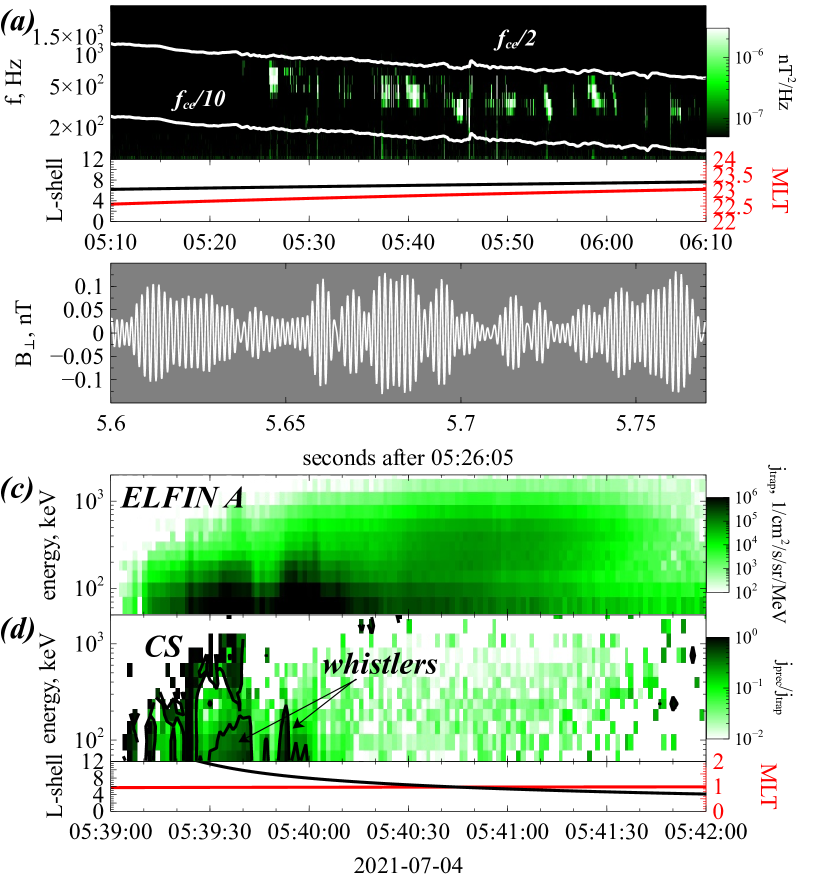
Figure 43: Overview of the event with the effect of nonlinear cyclotron resonance: near-equatorial THEMIS observations of whistler-mode magnetic field (a, b), low altitude ELFIN observations of trapped fluxes (c) and precipitating-to-trapped flux ratio (d). The precipitation burst due to electron scattering by whistler-mode waves is embedded into the dispersive precipitation structure (higher energies of precipitating electrons closer to the Earth) due to electron scattering by the magnetotail current sheet (CS) [see details in Artemyev et al., 2023; Wilkins et al., 2023].

Electron scattering by whistlers may significantly decrease electron pitch-angles and move particles to the loss-cone. An accurate estimate of the loss-cone size for the near-Earth magnetotail (injection region) is almost impossible, because empirical magnetic field models [Tsyganenko, 1995; Tsyganenko & Sitnov, 2007; Andreeva & Tsyganenko, 2019], with only few exceptions [Stephens et al., 2019; Sitnov et al., 2021; Tsyganenko et al., 2021], do not include the effects of dipolarization associated with plasma injection and strong variations of the equatorial magnetic field (such variations may significantly change the loss-cone size and precipitating electron fluxes, see, e.g. [Eshetu et al., 2018]). Typical loss-cone angle $\alpha_{LC}$ estimates give $\leq 2^{\circ}$ in the magnetotail (see Fig. 3(d) in Zhang et al. [2015]), and this value can be larger closer to the Earth. For a simulation of precipitating electron fluxes, we use $\alpha_{LC}=3^{\circ}$. This value could overestimate the precipitating flux magnitude, but there is almost no energy change due to the wave-particle resonant interaction at pitch-angles $<3$ degrees. Therefore, the energy spectrum of precipitating electrons derived from our simulation should reproduce the expected spectrum of electrons precipitating from the dipolarizing flux bundle region. To check this, we compare model results with observations from the low-altitude, polar-orbiting CubeSats ELFIN Angelopoulos et al. [2020] that provide conjugate measurements for the event in Fig. 43. Figure 43 shows an overview of ELFIN A trapped and precipitating fluxes: pattern of strong $j_{trap}$ increase at the inner edge of the plasma sheet (05:39:00-05:39:45 for ELFIN A) is also associated with a high ratio $j_{loss}/j_{trap}\sim 1$ showing strong energy dispersion: larger energies with $j_{loss}/j_{trap}\sim 1$ are closer to the Earth). This pattern most likely corresponds to the electron isotropic boundary Imhof et al. [1979]; Yahnin et al. [1997]; Sergeev et al. [2012]; Wilkins et al. [2023] , i.e., energetic electron scattering in the current sheet due to the magnetic field line curvature Birmingham [1984]; Büchner & Zelenyi [1989]; Young et al. [2002]; Lukin et al. [2021]. The curvature scattering efficiency depends on energy and on the equatorial magnetic field curvature radius and intensity. These dependencies are responsible for the observed energy dispersion Sergeev et al. [2018]; Dubyagin et al. [2021]. Closer to the Earth, ELFIN shows both a secondary burst of $j_{loss}/j_{trap}\sim 1$ and an increase of $j_{trap}$ (around 05:39:55), and this second precipitation pattern is not due to electron curvature scattering, because the energies of precipitating electrons are lower than energies of the pattern associated with the isotropic boundary observed farther away from the Earth. For ELFIN A this second precipitation pattern is observed around its conjunction to the equatorial injection region observed by THEMIS. We thus attribute this pattern to electron scattering from the injection region. Figure 44(b) shows spectra of precipitating electrons. Their average spectral shape is similar to the precipitating electron fluxes derived from the simulation driven by THEMIS equatorial measurements of electron fluxes and whistlers (compare red and grey curves). Therefore, our simulation confirms that the mapping technique can reproduce electron resonant interactions with field-aligned whistler-mode waves.

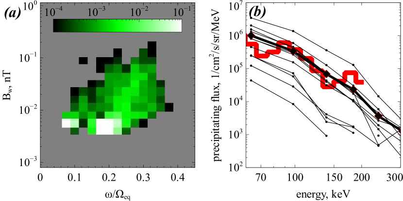
Figure 44: Panels (a) shows the distribution of wave amplitudes and frequencies for the event in Fig. 43. Panel (b) shows energy spectra from ELFIN A for the time interval associated with enhanced electron precipitations. The red curve shows the model result.

References

- (1)
- Åsnes et al. (2005) Åsnes, A., Friedel, R. W., Stadsnes, J., Thomsen, M., Østgaard, N. & Cayton, T. (2005), ‘Statistical pitch angle properties of substorm-injected electron clouds and their relation to dawnside energetic electron precipitation’, J. Geophys. Res. 110, 5207.
- Agapitov et al. (2013) Agapitov, O. V., Artemyev, A., Krasnoselskikh, V., Khotyaintsev, Y. V., Mourenas, D., Breuillard, H., Balikhin, M. & Rolland, G. (2013), ‘Statistics of whistler mode waves in the outer radiation belt: Cluster STAFF-SA measurements’, J. Geophys. Res. 118, 3407–3420.
- Agapitov et al. (2014) Agapitov, O. V., Artemyev, A., Mourenas, D., Krasnoselskikh, V., Bonnell, J., Le Contel, O., Cully, C. M. & Angelopoulos, V. (2014), ‘The quasi-electrostatic mode of chorus waves and electron nonlinear acceleration’, J. Geophys. Res. 119, 1606–1626.
- Agapitov et al. (2015a) Agapitov, O. V., Artemyev, A. V., Mourenas, D., Mozer, F. S. & Krasnoselskikh, V. (2015a), ‘Empirical model of lower band chorus wave distribution in the outer radiation belt’, J. Geophys. Res. 120, 10.
- Agapitov et al. (2015b) Agapitov, O. V., Artemyev, A. V., Mourenas, D., Mozer, F. S. & Krasnoselskikh, V. (2015b), ‘Nonlinear local parallel acceleration of electrons through Landau trapping by oblique whistler mode waves in the outer radiation belt’, Geophys. Res. Lett. 42, 10.
-
Agapitov et al. (2016)
Agapitov, O. V., Mourenas, D., Artemyev, A. V. & Mozer,
F. S. (2016), ‘Exclusion principle for very
oblique and parallel lower band chorus waves’, Geophys. Res. Lett. 43(21), 11,112–11,120.
http://dx.doi.org/10.1002/2016GL071250 - Agapitov et al. (2018) Agapitov, O. V., Mourenas, D., Artemyev, A. V., Mozer, F. S., Hospodarsky, G., Bonnell, J. & Krasnoselskikh, V. (2018), ‘Synthetic Empirical Chorus Wave Model From Combined Van Allen Probes and Cluster Statistics’, Journal of Geophysical Research (Space Physics) 123(1), 297–314.
- Albert (1993) Albert, J. M. (1993), ‘Cyclotron resonance in an inhomogeneous magnetic field’, Physics of Fluids B 5, 2744–2750.
- Albert (2000) Albert, J. M. (2000), ‘Gyroresonant interactions of radiation belt particles with a monochromatic electromagnetic wave’, J. Geophys. Res. 105, 21191.
- Albert (2001) Albert, J. M. (2001), ‘Comparison of pitch angle diffusion by turbulent and monochromatic whistler waves’, J. Geophys. Res. 106, 8477–8482.
- Albert (2010) Albert, J. M. (2010), ‘Diffusion by one wave and by many waves’, J. Geophys. Res. 115, 0.
- Albert (2017) Albert, J. M. (2017), ‘Quasi-linear diffusion coefficients for highly oblique whistler mode waves’, J. Geophys. Res. 122, 5339–5354.
- Albert (2018) Albert, J. M. (2018), ‘Diagonalization of diffusion equations in two and three dimensions’, Journal of Atmospheric and Solar-Terrestrial Physics 177, 202–207.
- Albert et al. (2022) Albert, J. M., Artemyev, A., Li, W., Gan, L. & Ma, Q. (2022), ‘Analytical results for phase bunching in the pendulum model of wave-particle interactions’, Frontiers in Astronomy and Space Sciences 9, 971358.
- Albert et al. (2021) Albert, J. M., Artemyev, A. V., Li, W., Gan, L. & Ma, Q. (2021), ‘Models of resonant wave-particle interactions’, Journal of Geophysical Research: Space Physics 126(6), e2021JA029216.
- Albert & Bortnik (2009) Albert, J. M. & Bortnik, J. (2009), ‘Nonlinear interaction of radiation belt electrons with electromagnetic ion cyclotron waves’, Geophys. Res. Lett. 36, 12110.
- Albert et al. (2013) Albert, J. M., Tao, X. & Bortnik, J. (2013), Aspects of Nonlinear Wave-Particle Interactions, in D. Summers, I. U. Mann, D. N. Baker & M. Schulz, eds, ‘Dynamics of the Earth’s Radiation Belts and Inner Magnetosphere’, American Geophysical Union.
- Alekhin & Shklyar (1980) Alekhin, J. K. & Shklyar, D. R. (1980), ‘Some questions of VLF wave propagation in the magnetosphere’, Geomagnetism and Aeronomy/Geomagnetizm i Aeronomiia 20, 501–507.
- Allanson et al. (2024) Allanson, O., Ma, D., Osmane, A., Albert, J. M., Bortnik, J., Watt, C. E. J., Chapman, S. C., Spencer, J., Ratliff, D. J., Meredith, N. P., Elsden, T., Neukirch, T., Hartley, D. P., Black, R., Watkins, N. W. & Elvidge, S. (2024), ‘The challenge to understand the zoo of particle transport regimes during resonant wave-particle interactions for given survey-mode wave spectra’, Frontiers in Astronomy and Space Sciences 11, 1332931.
- Allanson et al. (2022) Allanson, O., Thomas, E., Watt, C. E. J. & Neukirch, T. (2022), ‘Weak Turbulence and Quasilinear Diffusion for Relativistic Wave-Particle Interactions Via a Markov Approach’, Frontiers in Physics 8:805699.
- Allanson et al. (2021) Allanson, O., Watt, C. E. J., Allison, H. J. & Ratcliffe, H. (2021), ‘Electron Diffusion and Advection During Nonlinear Interactions With Whistler Mode Waves’, Journal of Geophysical Research (Space Physics) 126(5), e28793.
- Allanson et al. (2020) Allanson, O., Watt, C. E. J., Ratcliffe, H., Allison, H. J., Meredith, N. P., Bentley, S. N., Ross, J. P. J. & Glauert, S. A. (2020), ‘Particle-in-Cell Experiments Examine Electron Diffusion by Whistler-Mode Waves: 2. Quasi-Linear and Nonlinear Dynamics’, Journal of Geophysical Research (Space Physics) 125(7), e27949.
- Allanson et al. (2019) Allanson, O., Watt, C. E. J., Ratcliffe, H., Meredith, N. P., Allison, H. J., Bentley, S. N., Bloch, T. & Glauert, S. A. (2019), ‘Particle-in-cell Experiments Examine Electron Diffusion by Whistler-mode Waves: 1. Benchmarking With a Cold Plasma’, Journal of Geophysical Research (Space Physics) 124(11), 8893–8912.
- Allison & Shprits (2020) Allison, H. J. & Shprits, Y. Y. (2020), ‘Local heating of radiation belt electrons to ultra-relativistic energies’, Nature Communications 11, 4533.
- An et al. (2024) An, X., Artemyev, A., Angelopoulos, V., Zhang, X.-J., Mourenas, D., Bortnik, J. & Shi, X. (2024), ‘Nonresonant scattering of energetic electrons by electromagnetic ion cyclotron waves: Spacecraft observations and theoretical framework’, Journal of Geophysical Research: Space Physics 129(3), e2023JA031863.
- An, Artemyev, Angelopoulos, Zhang, Mourenas & Bortnik (2022) An, X., Artemyev, A., Angelopoulos, V., Zhang, X., Mourenas, D. & Bortnik, J. (2022), ‘Nonresonant Scattering of Relativistic Electrons by Electromagnetic Ion Cyclotron Waves in Earth’s Radiation Belts’, Phys. Rev. Lett 129(13), 135101.
- An, Wu & Tao (2022) An, Z., Wu, Y. & Tao, X. (2022), ‘Electron Dynamics in a Chorus Wave Field Generated From Particle-In-Cell Simulations’, Geophys. Res. Lett. 49(3), e97778.
- Andreeva & Tsyganenko (2019) Andreeva, V. A. & Tsyganenko, N. A. (2019), ‘Empirical Modeling of the Geomagnetosphere for SIR and CME-Driven Magnetic Storms’, Journal of Geophysical Research (Space Physics) 124(7), 5641–5662.
- Angelopoulos (2008) Angelopoulos, V. (2008), ‘The THEMIS Mission’, Space Sci. Rev. 141, 5–34.
- Angelopoulos et al. (2008) Angelopoulos, V., Sibeck, D., Carlson, C. W., McFadden, J. P., Larson, D., Lin, R. P., Bonnell, J. W., Mozer, F. S., Ergun, R., Cully, C., Glassmeier, K. H., Auster, U., Roux, A., Lecontel, O., Frey, S., Phan, T., Mende, S., Frey, H., Donovan, E., Russell, C. T., Strangeway, R., Liu, J., Mann, I., Rae, J., Raeder, J., Li, X., Liu, W., Singer, H. J., Sergeev, V. A., Apatenkov, S., Parks, G., Fillingim, M. & Sigwarth, J. (2008), ‘First Results from the THEMIS Mission’, Space Sci. Rev. 141, 453–476.
- Angelopoulos et al. (2020) Angelopoulos, V., Tsai, E., Bingley, L., Shaffer, C., Turner, D. L., Runov, A., Li, W., Liu, J., Artemyev, A. V., Zhang, X. J., Strangeway, R. J., Wirz, R. E., Shprits, Y. Y., Sergeev, V. A., Caron, R. P., Chung, M., Cruce, P., Greer, W., Grimes, E., Hector, K., Lawson, M. J., Leneman, D., Masongsong, E. V., Russell, C. L., Wilkins, C., Hinkley, D., Blake, J. B., Adair, N., Allen, M., Anderson, M., Arreola-Zamora, M., Artinger, J., Asher, J., Branchevsky, D., Capitelli, M. R., Castro, R., Chao, G., Chung, N., Cliffe, M., Colton, K., Costello, C., Depe, D., Domae, B. W., Eldin, S., Fitzgibbon, L., Flemming, A., Fox, I., Frederick, D. M., Gilbert, A., Gildemeister, A., Gonzalez, A., Hesford, B., Jha, S., Kang, N., King, J., Krieger, R., Lian, K., Mao, J., McKinney, E., Miller, J. P., Norris, A., Nuesca, M., Palla, A., Park, E. S. Y., Pedersen, C. E., Qu, Z., Rozario, R., Rye, E., Seaton, R., Subramanian, A., Sundin, S. R., Tan, A., Turner, W., Villegas, A. J., Wasden, M., Wing, G., Wong, C., Xie, E., Yamamoto, S., Yap, R., Zarifian, A. & Zhang, G. Y. (2020), ‘The ELFIN Mission’, Space Sci. Rev. 216(5), 103.
- Angelopoulos et al. (2023) Angelopoulos, V., Zhang, X. J., Artemyev, A. V., Mourenas, D., Tsai, E., Wilkins, C., Runov, A., Liu, J., Turner, D. L., Li, W., Khurana, K., Wirz, R. E., Sergeev, V. A., Meng, X., Wu, J., Hartinger, M. D., Raita, T., Shen, Y., An, X., Shi, X., Bashir, M. F., Shen, X., Gan, L., Qin, M., Capannolo, L., Ma, Q., Russell, C. L., Masongsong, E. V., Caron, R., He, I., Iglesias, L., Jha, S., King, J., Kumar, S., Le, K., Mao, J., McDermott, A., Nguyen, K., Norris, A., Palla, A., Roosnovo, A., Tam, J., Xie, E., Yap, R. C., Ye, S., Young, C., Adair, L. A., Shaffer, C., Chung, M., Cruce, P., Lawson, M., Leneman, D., Allen, M., Anderson, M., Arreola-Zamora, M., Artinger, J., Asher, J., Branchevsky, D., Cliffe, M., Colton, K., Costello, C., Depe, D., Domae, B. W., Eldin, S., Fitzgibbon, L., Flemming, A., Frederick, D. M., Gilbert, A., Hesford, B., Krieger, R., Lian, K., McKinney, E., Miller, J. P., Pedersen, C., Qu, Z., Rozario, R., Rubly, M., Seaton, R., Subramanian, A., Sundin, S. R., Tan, A., Thomlinson, D., Turner, W., Wing, G., Wong, C. & Zarifian, A. (2023), ‘Energetic Electron Precipitation Driven by Electromagnetic Ion Cyclotron Waves from ELFIN’s Low Altitude Perspective’, Space Sci. Rev. 219(5), 37.
- Arnold et al. (2006) Arnold, V. I., Kozlov, V. V. & Neishtadt, A. I. (2006), Mathematical Aspects of Classical and Celestial Mechanics, Dynamical Systems III. Encyclopedia of Mathematical Sciences, 3rd edn, Springer-Verlag, New York.
- Artemyev, Agapitov, Mourenas, Krasnoselskikh, Shastun & Mozer (2016) Artemyev, A. V., Agapitov, O., Mourenas, D., Krasnoselskikh, V., Shastun, V. & Mozer, F. (2016), ‘Oblique Whistler-Mode Waves in the Earth’s Inner Magnetosphere: Energy Distribution, Origins, and Role in Radiation Belt Dynamics’, Space Sci. Rev. 200(1-4), 261–355.
- Artemyev, Agapitov, Mourenas, Krasnoselskikh & Mozer (2015) Artemyev, A. V., Agapitov, O. V., Mourenas, D., Krasnoselskikh, V. V. & Mozer, F. S. (2015), ‘Wave energy budget analysis in the Earth’s radiation belts uncovers a missing energy’, Nature Communications 6, 8143.
- Artemyev, Agapitov, Mourenas, Krasnoselskikh & Zelenyi (2013) Artemyev, A. V., Agapitov, O. V., Mourenas, D., Krasnoselskikh, V. & Zelenyi, L. M. (2013), ‘Storm-induced energization of radiation belt electrons: Effect of wave obliquity’, Geophys. Res. Lett. 40, 4138–4143.
- Artemyev et al. (2023) Artemyev, A. V., Angelopoulos, V., Zhang, X. J., Chen, L. & Runov, A. (2023), ‘Dispersed Relativistic Electron Precipitation Patterns Between the Ion and Electron Isotropy Boundaries’, Journal of Geophysical Research (Space Physics) 128(12), e2023JA032200.
- Artemyev, Demekhov, Zhang, Angelopoulos, Mourenas, Fedorenko, Maninnen, Tsai, Wilkins, Kasahara, Miyoshi, Matsuoka, Kasahara, Mitani, Yokota, Keika, Hori, Matsuda, Nakamura, Kitahara, Takashima & Shinohara (2021) Artemyev, A. V., Demekhov, A. G., Zhang, X. J., Angelopoulos, V., Mourenas, D., Fedorenko, Y. V., Maninnen, J., Tsai, E., Wilkins, C., Kasahara, S., Miyoshi, Y., Matsuoka, A., Kasahara, Y., Mitani, T., Yokota, S., Keika, K., Hori, T., Matsuda, S., Nakamura, S., Kitahara, M., Takashima, T. & Shinohara, I. (2021), ‘Role of Ducting in Relativistic Electron Loss by Whistler-Mode Wave Scattering’, Journal of Geophysical Research (Space Physics) 126(11), e29851.
- Artemyev et al. (2012) Artemyev, A. V., Krasnoselskikh, V., Agapitov, O., Mourenas, D. & Rolland, G. (2012), ‘Non-diffusive resonant acceleration of electrons in the radiation belts.’, Physics of Plasmas 19, 122901.
- Artemyev & Mourenas (2020) Artemyev, A. V. & Mourenas, D. (2020), ‘On Whistler Mode Wave Relation to Electron Field-Aligned Plateau Populations’, Journal of Geophysical Research (Space Physics) 125(3), e27735.
- Artemyev, Mourenas, Agapitov, Vainchtein, Mozer & Krasnoselskikh (2015) Artemyev, A. V., Mourenas, D., Agapitov, O. V., Vainchtein, D. L., Mozer, F. S. & Krasnoselskikh, V. V. (2015), ‘Stability of relativistic electron trapping by strong whistler or electromagnetic ion cyclotron waves’, Physics of Plasmas 22, 082901.
- Artemyev, Mourenas, Zhang & Vainchtein (2022) Artemyev, A. V., Mourenas, D., Zhang, X. J. & Vainchtein, D. (2022), ‘On the Incorporation of Nonlinear Resonant Wave-Particle Interactions Into Radiation Belt Models’, Journal of Geophysical Research (Space Physics) 127(9), e30853.
- Artemyev, Neishtadt, Albert, Gan, Li & Ma (2021) Artemyev, A. V., Neishtadt, A. I., Albert, J. M., Gan, L., Li, W. & Ma, Q. (2021), ‘Theoretical model of the nonlinear resonant interaction of whistler-mode waves and field-aligned electrons’, Physics of Plasmas 28(5), 052902.
- Artemyev, Neishtadt & Angelopoulos (2022) Artemyev, A. V., Neishtadt, A. I. & Angelopoulos, V. (2022), ‘On the Role of Whistler-Mode Waves in Electron Interaction With Dipolarizing Flux Bundles’, Journal of Geophysical Research (Space Physics) 127(4), e30265.
- Artemyev, Neishtadt, Vainchtein, Vasiliev, Vasko & Zelenyi (2018) Artemyev, A. V., Neishtadt, A. I., Vainchtein, D. L., Vasiliev, A. A., Vasko, I. Y. & Zelenyi, L. M. (2018), ‘Trapping (capture) into resonance and scattering on resonance: Summary of results for space plasma systems’, Communications in Nonlinear Science and Numerical Simulations 65, 111–160.
- Artemyev, Neishtadt & Vasiliev (2019) Artemyev, A. V., Neishtadt, A. I. & Vasiliev, A. A. (2019), ‘Kinetic equation for nonlinear wave-particle interaction: Solution properties and asymptotic dynamics’, Physica D Nonlinear Phenomena 393, 1–8.
- Artemyev, Neishtadt & Vasiliev (2020a) Artemyev, A. V., Neishtadt, A. I. & Vasiliev, A. A. (2020a), ‘A Map for Systems with Resonant Trappings and Scatterings’, Regular and Chaotic Dynamics 25(1), 2–10.
- Artemyev, Neishtadt & Vasiliev (2020b) Artemyev, A. V., Neishtadt, A. I. & Vasiliev, A. A. (2020b), ‘Mapping for nonlinear electron interaction with whistler-mode waves’, Physics of Plasmas 27(4), 042902.
- Artemyev, Neishtadt & Vasiliev (2021) Artemyev, A. V., Neishtadt, A. I. & Vasiliev, A. A. (2021), Kinetic Equation for Systems with Resonant Captures and Scatterings, Springer Singapore, Singapore, pp. 171–180.
- Artemyev, Neishtadt, Vasiliev & Mourenas (2016) Artemyev, A. V., Neishtadt, A. I., Vasiliev, A. A. & Mourenas, D. (2016), ‘Kinetic equation for nonlinear resonant wave-particle interaction’, Physics of Plasmas 23(9), 090701.
- Artemyev et al. (2017a) Artemyev, A. V., Neishtadt, A. I., Vasiliev, A. A. & Mourenas, D. (2017a), ‘Kinetic equation for systems with resonant captures and scatterings’, ArXiv e-prints .
- Artemyev et al. (2017b) Artemyev, A. V., Neishtadt, A. I., Vasiliev, A. A. & Mourenas, D. (2017b), ‘Probabilistic approach to nonlinear wave-particle resonant interaction’, Phys. Rev. E 95(2), 023204.
- Artemyev, Neishtadt, Vasiliev & Mourenas (2018) Artemyev, A. V., Neishtadt, A. I., Vasiliev, A. A. & Mourenas, D. (2018), ‘Long-term evolution of electron distribution function due to nonlinear resonant interaction with whistler mode waves’, Journal of Plasma Physics 84, 905840206.
- Artemyev, Neishtadt, Vasiliev & Mourenas (2021) Artemyev, A. V., Neishtadt, A. I., Vasiliev, A. A. & Mourenas, D. (2021), ‘Transitional regime of electron resonant interaction with whistler-mode waves in inhomogeneous space plasma’, Phys. Rev. E 104(5), 055203.
- Artemyev, Neishtadt, Vasiliev, Zhang, Mourenas & Vainchtein (2021) Artemyev, A. V., Neishtadt, A. I., Vasiliev, A. A., Zhang, X.-J., Mourenas, D. & Vainchtein, D. (2021), ‘Long-term dynamics driven by resonant wave-particle interactions: from Hamiltonian resonance theory to phase space mapping’, Journal of Plasma Physics 87(2), 835870201.
- Artemyev, Orlova, Mourenas, Agapitov & Krasnoselskikh (2013) Artemyev, A. V., Orlova, K. G., Mourenas, D., Agapitov, O. V. & Krasnoselskikh, V. V. (2013), ‘Electron pitch-angle diffusion: resonant scattering by waves vs. nonadiabatic effects’, Annales Geophysicae 31, 1485–1490.
- Artemyev et al. (2011) Artemyev, A. V., Vainchtein, D., Neishtadt, A. & Zelenyi, L. (2011), ‘Resonant acceleration of charged particles in the presence of random fluctuations’, Phys. Rev. E 84(4), 046213.
- Artemyev, Vasiliev, Mourenas, Agapitov & Krasnoselskikh (2013) Artemyev, A. V., Vasiliev, A. A., Mourenas, D., Agapitov, O. & Krasnoselskikh, V. (2013), ‘Nonlinear electron acceleration by oblique whistler waves: Landau resonance vs. cyclotron resonance.’, Physics of Plasmas 20, 122901.
- Artemyev, Vasiliev, Mourenas, Agapitov, Krasnoselskikh, Boscher & Rolland (2014) Artemyev, A. V., Vasiliev, A. A., Mourenas, D., Agapitov, O., Krasnoselskikh, V., Boscher, D. & Rolland, G. (2014), ‘Fast transport of resonant electrons in phase space due to nonlinear trapping by whistler waves’, Geophys. Res. Lett. 41, 5727–5733.
- Artemyev, Vasiliev, Mourenas, Agapitov & Krasnoselskikh (2014) Artemyev, A. V., Vasiliev, A. A., Mourenas, D., Agapitov, O. V. & Krasnoselskikh, V. V. (2014), ‘Electron scattering and nonlinear trapping by oblique whistler waves: The critical wave intensity for nonlinear effects’, Physics of Plasmas 21(10), 102903.
- Artemyev, Vasiliev, Mourenas, Neishtadt, Agapitov & Krasnoselskikh (2015) Artemyev, A. V., Vasiliev, A. A., Mourenas, D., Neishtadt, A. I., Agapitov, O. V. & Krasnoselskikh, V. (2015), ‘Probability of relativistic electron trapping by parallel and oblique whistler-mode waves in Earth’s radiation belts’, Physics of Plasmas 22(11), 112903.
- Artemyev, Vasiliev & Neishtadt (2019) Artemyev, A. V., Vasiliev, A. A. & Neishtadt, A. I. (2019), ‘Charged particle nonlinear resonance with localized electrostatic wave-packets’, Communications in Nonlinear Science and Numerical Simulations 72, 392–406.
- Artemyev, Zhang, Angelopoulos, Mourenas, Vainchtein, Shen, Vasko & Runov (2020) Artemyev, A. V., Zhang, X. J., Angelopoulos, V., Mourenas, D., Vainchtein, D., Shen, Y., Vasko, I. & Runov, A. (2020), ‘Ionosphere Feedback to Electron Scattering by Equatorial Whistler Mode Waves’, Journal of Geophysical Research (Space Physics) 125(9), e28373.
- Artemyev et al. (2024) Artemyev, A. V., Zhang, X. J., Demekhov, A. G., Meng, X., Angelopoulos, V. & Fedorenko, Y. V. (2024), ‘Relativistic Electron Precipitation Driven by Mesoscale Transients, Inferred From Ground and Multi-Spacecraft Platforms’, Journal of Geophysical Research (Space Physics) 129(2), e2023JA032287.
- Artemyev, Zhang, Zou, Mourenas, Angelopoulos, Vainchtein, Tsai & Wilkins (2022) Artemyev, A. V., Zhang, X. J., Zou, Y., Mourenas, D., Angelopoulos, V., Vainchtein, D., Tsai, E. & Wilkins, C. (2022), ‘On the Nature of Intense Sub-Relativistic Electron Precipitation’, Journal of Geophysical Research (Space Physics) 127(6), e30571.
- Auster et al. (2008) Auster, H. U., Glassmeier, K. H., Magnes, W., Aydogar, O., Baumjohann, W., Constantinescu, D., Fischer, D., Fornacon, K. H., Georgescu, E., Harvey, P., Hillenmaier, O., Kroth, R., Ludlam, M., Narita, Y., Nakamura, R., Okrafka, K., Plaschke, F., Richter, I., Schwarzl, H., Stoll, B., Valavanoglou, A. & Wiedemann, M. (2008), ‘The THEMIS Fluxgate Magnetometer’, Space Sci. Rev. 141, 235–264.
- Baker et al. (2018) Baker, D. N., Erickson, P. J., Fennell, J. F., Foster, J. C., Jaynes, A. N. & Verronen, P. T. (2018), ‘Space Weather Effects in the Earth’s Radiation Belts’, Space Sci. Rev. 214(1), 17.
- Baker et al. (2014) Baker, D. N., Jaynes, A. N., Hoxie, V. C., Thorne, R. M., Foster, J. C., Li, X., Fennell, J. F., Wygant, J. R., Kanekal, S. G., Erickson, P. J., Kurth, W., Li, W., Ma, Q., Schiller, Q., Blum, L., Malaspina, D. M., Gerrard, A. & Lanzerotti, L. J. (2014), ‘An impenetrable barrier to ultrarelativistic electrons in the Van Allen radiation belts’, Nature 515(7528), 531–534.
- Baker et al. (2016) Baker, D. N., Jaynes, A. N., Kanekal, S. G., Foster, J. C., Erickson, P. J., Fennell, J. F., Blake, J. B., Zhao, H., Li, X., Elkington, S. R., Henderson, M. G., Reeves, G. D., Spence, H. E., Kletzing, C. A. & Wygant, J. R. (2016), ‘Highly relativistic radiation belt electron acceleration, transport, and loss: Large solar storm events of March and June 2015’, Journal of Geophysical Research (Space Physics) 121(7), 6647–6660.
- Baker et al. (2013) Baker, D. N., Kanekal, S. G., Hoxie, V. C., Batiste, S., Bolton, M., Li, X., Elkington, S. R., Monk, S., Reukauf, R., Steg, S., Westfall, J., Belting, C., Bolton, B., Braun, D., Cervelli, B., Hubbell, K., Kien, M., Knappmiller, S., Wade, S., Lamprecht, B., Stevens, K., Wallace, J., Yehle, A., Spence, H. E. & Friedel, R. (2013), ‘The Relativistic Electron-Proton Telescope (REPT) Instrument on Board the Radiation Belt Storm Probes (RBSP) Spacecraft: Characterization of Earth’s Radiation Belt High-Energy Particle Populations’, Space Sci. Rev. 179, 337–381.
- Bell (1984) Bell, T. F. (1984), ‘The nonlinear gyroresonance interaction between energetic electrons and coherent VLF waves propagating at an arbitrary angle with respect to the earth’s magnetic field’, J. Geophys. Res. 89, 905–918.
- Bell (1986) Bell, T. F. (1986), ‘The wave magnetic field amplitude threshold for nonlinear trapping of energetic gyroresonant and Landau resonant electrons by nonducted VLF waves in the magnetosphere’, J. Geophys. Res. 91, 4365–4379.
- Bell et al. (2002) Bell, T. F., Inan, U. S., Bortnik, J. & Scudder, J. D. (2002), ‘The Landau damping of magnetospherically reflected whistlers within the plasmasphere’, Geophys. Res. Lett. 29, 1733.
- Benkadda et al. (1996) Benkadda, S., Sen, A. & Shklyar, D. R. (1996), ‘Chaotic dynamics of charged particles in the field of two monochromatic waves in a magnetized plasma’, Chaos 6(3), 451–460.
- Birmingham (1984) Birmingham, T. J. (1984), ‘Pitch angle diffusion in the Jovian magnetodisc’, J. Geophys. Res. 89, 2699–2707.
- Blake et al. (2013) Blake, J. B., Carranza, P. A., Claudepierre, S. G., Clemmons, J. H., Crain, W. R., Dotan, Y., Fennell, J. F., Fuentes, F. H., Galvan, R. M., George, J. S., Henderson, M. G., Lalic, M., Lin, A. Y., Looper, M. D., Mabry, D. J., Mazur, J. E., McCarthy, B., Nguyen, C. Q., O’Brien, T. P., Perez, M. A., Redding, M. T., Roeder, J. L., Salvaggio, D. J., Sorensen, G. A., Spence, H. E., Yi, S. & Zakrzewski, M. P. (2013), ‘The Magnetic Electron Ion Spectrometer (MagEIS) Instruments Aboard the Radiation Belt Storm Probes (RBSP) Spacecraft’, Space Sci. Rev. 179, 383–421.
- Bonnell et al. (2008) Bonnell, J. W., Mozer, F. S., Delory, G. T., Hull, A. J., Ergun, R. E., Cully, C. M., Angelopoulos, V. & Harvey, P. R. (2008), ‘The Electric Field Instrument (EFI) for THEMIS’, Space Sci. Rev. 141, 303–341.
- Bortnik et al. (2022) Bortnik, J., Albert, J. M., Artemyev, A., Li, W., Jun, C.-W., Grach, V. S. & Demekhov, A. G. (2022), ‘Amplitude Dependence of Nonlinear Precipitation Blocking of Relativistic Electrons by Large Amplitude EMIC Waves’, Geophys. Res. Lett. 49(12), e98365.
- Bortnik et al. (2006) Bortnik, J., Inan, U. S. & Bell, T. F. (2006), ‘Landau damping and resultant unidirectional propagation of chorus waves’, Geophys. Res. Lett. 33, 3102.
- Bortnik & Thorne (2010) Bortnik, J. & Thorne, R. M. (2010), ‘Transit time scattering of energetic electrons due to equatorially confined magnetosonic waves’, J. Geophys. Res. 115, 7213.
- Bortnik et al. (2008) Bortnik, J., Thorne, R. M. & Inan, U. S. (2008), ‘Nonlinear interaction of energetic electrons with large amplitude chorus’, Geophys. Res. Lett. 35, 21102.
- Bortnik et al. (2007) Bortnik, J., Thorne, R. M., Meredith, N. P. & Santolik, O. (2007), ‘Ray tracing of penetrating chorus and its implications for the radiation belts’, Geophys. Res. Lett. 34, L15109.
- Bortnik et al. (2015) Bortnik, J., Thorne, R. M., Ni, B. & Li, J. (2015), ‘Analytical approximation of transit time scattering due to magnetosonic waves’, Geophys. Res. Lett. 42, 1318–1325.
- Breuillard et al. (2014) Breuillard, H., Agapitov, O., Artemyev, A., Krasnoselskikh, V., Le Contel, O., Cully, C. M., Angelopoulos, V., Zaliznyak, Y. & Rolland, G. (2014), ‘On the origin of falling-tone chorus elements in Earth’s inner magnetosphere’, Annales Geophysicae 32, 1477–1485.
- Breuillard et al. (2016) Breuillard, H., Le Contel, O., Retino, A., Chasapis, A., Chust, T., Mirioni, L., Graham, D. B., Wilder, F. D., Cohen, I., Vaivads, A., Khotyaintsev, Y. V., Lindqvist, P.-A., Marklund, G. T., Burch, J. L., Torbert, R. B., Ergun, R. E., Goodrich, K. A., Macri, J., Needell, J., Chutter, M., Rau, D., Dors, I., Russell, C. T., Magnes, W., Strangeway, R. J., Bromund, K. R., Plaschke, F., Fischer, D., Leinweber, H. K., Anderson, B. J., Le, G., Slavin, J. A., Kepko, E. L., Baumjohann, W., Mauk, B., Fuselier, S. A. & Nakamura, R. (2016), ‘Multispacecraft analysis of dipolarization fronts and associated whistler wave emissions using MMS data’, Geophys. Res. Lett. 43, 7279–7286.
- Breuillard et al. (2012) Breuillard, H., Zaliznyak, Y., Krasnoselskikh, V., Agapitov, O., Artemyev, A. & Rolland, G. (2012), ‘Chorus wave-normal statistics in the Earth’s radiation belts from ray tracing technique’, Ann. Geophys. 30, 1223–1233.
- Brinca (1978) Brinca, A. L. (1978), ‘Turbulence effects in the cyclotron resonance of monochromatic whistlers’, Geophys. Res. Lett. 5, 839–842.
- Brinca (1980) Brinca, A. L. (1980), ‘On the evolution of the geomagnetospheric coherent cyclotron resonance in the midst of noise’, J. Geophys. Res. 85, 4711–4714.
- Brizard (2023) Brizard, A. J. (2023), ‘Variational formulation of higher-order guiding-center Vlasov-Maxwell theory’, Physics of Plasmas 30(10), 102106.
- Brizard & Chan (2022) Brizard, A. J. & Chan, A. A. (2022), ‘Hamiltonian formulations of quasilinear theory for magnetized plasmas’, Frontiers in Astronomy and Space Sciences 9, 1010133.
- Büchner & Zelenyi (1989) Büchner, J. & Zelenyi, L. M. (1989), ‘Regular and chaotic charged particle motion in magnetotaillike field reversals. I - Basic theory of trapped motion’, J. Geophys. Res. 94, 11821–11842.
- Burton & Holzer (1974) Burton, R. K. & Holzer, R. E. (1974), ‘The Origin and Propagation of Chorus in the Outer Magnetosphere’, J. Geophys. Res. 79, 1014–1023.
- Cai et al. (2020) Cai, B., Wu, Y. & Tao, X. (2020), ‘Effects of Nonlinear Resonance Broadening on Interactions Between Electrons and Whistler Mode Waves’, Geophys. Res. Lett. 47(11), e87991.
- Camporeale (2015) Camporeale, E. (2015), ‘Resonant and nonresonant whistlers-particle interaction in the radiation belts’, Geophys. Res. Lett. 42(9), 3114–3121.
- Camporeale & Zimbardo (2015) Camporeale, E. & Zimbardo, G. (2015), ‘Wave-particle interactions with parallel whistler waves: Nonlinear and time-dependent effects revealed by particle-in-cell simulations’, Physics of Plasmas 22(9), 092104.
- Capannolo et al. (2023) Capannolo, L., Li, W., Ma, Q., Qin, M., Shen, X. C., Angelopoulos, V., Artemyev, A., Zhang, X. J. & Hanzelka, M. (2023), ‘Electron Precipitation Observed by ELFIN Using Proton Precipitation as a Proxy for Electromagnetic Ion Cyclotron (EMIC) Waves’, Geophys. Res. Lett. 50(21), e2023GL103519.
- Cary & Brizard (2009) Cary, J. R. & Brizard, A. J. (2009), ‘Hamiltonian theory of guiding-center motion’, Reviews of Modern Physics 81, 693–738.
- Cattell et al. (2008) Cattell, C., Wygant, J. R., Goetz, K., Kersten, K., Kellogg, P. J., von Rosenvinge, T., Bale, S. D., Roth, I., Temerin, M., Hudson, M. K., Mewaldt, R. A., Wiedenbeck, M., Maksimovic, M., Ergun, R., Acuna, M. & Russell, C. T. (2008), ‘Discovery of very large amplitude whistler-mode waves in Earth’s radiation belts’, Geophys. Res. Lett. 35, 1105.
- Chan et al. (2023) Chan, A. A., Elkington, S. R., Longley, W. J., Aldhurais, S. A., Alam, S. S., Albert, J. M., Jaynes, A. N., Malaspina, D. M., Ma, Q. & Li, W. (2023), ‘Simulation of radiation belt wave-particle interactions in an mhd-particle framework’, Frontiers in Astronomy and Space Sciences 10.
- Chen et al. (2024) Chen, H., Wang, X., Chen, L., Zhang, X.-J., Omura, Y., Chen, R., Hsieh, Y.-K., Lin, Y. & Xia, Z. (2024), ‘Nonlinear Electron Trapping Through Cyclotron Resonance in the Formation of Chorus Subpackets’, Geophys. Res. Lett. 51(11), e2024GL109481.
- Chen et al. (2020) Chen, L., Breneman, A. W., Xia, Z. & Zhang, X.-j. (2020), ‘Modeling of Bouncing Electron Microbursts Induced by Ducted Chorus Waves’, Geophys. Res. Lett. 47(17), e89400.
- Chen et al. (2013) Chen, L., Thorne, R. M., Li, W. & Bortnik, J. (2013), ‘Modeling the wave normal distribution of chorus waves’, J. Geophys. Res. 118, 1074–1088.
- Chen et al. (2022) Chen, L., Zhang, X.-J., Artemyev, A., Angelopoulos, V., Tsai, E., Wilkins, C. & Horne, R. B. (2022), ‘Ducted Chorus Waves Cause Sub-Relativistic and Relativistic Electron Microbursts’, Geophys. Res. Lett. 49(5), e97559.
- Chen, Gao, Lu, Chen, Tsurutani, Li, Ni & Wang (2021) Chen, R., Gao, X., Lu, Q., Chen, L., Tsurutani, B. T., Li, W., Ni, B. & Wang, S. (2021), ‘In Situ Observations of Whistler Mode Chorus Waves Guided by Density Ducts’, Journal of Geophysical Research (Space Physics) 126(4), e28814.
- Chen, Gao, Lu, Tsurutani & Wang (2021) Chen, R., Gao, X., Lu, Q., Tsurutani, B. T. & Wang, S. (2021), ‘Observational Evidence for Whistler Mode Waves Guided/Ducted by the Inner and Outer Edges of the Plasmapause’, Geophys. Res. Lett. 48(6), e92652.
- Chen et al. (2019) Chen, R., Gao, X., Lu, Q. & Wang, S. (2019), ‘Unraveling the Correlation Between Chorus Wave and Electron Beam-Like Distribution in the Earth’s Magnetosphere’, Geophys. Res. Lett. 46(21), 11,671–11,678.
- Chen et al. (2007) Chen, Y., Reeves, G. D. & Friedel, R. H. W. (2007), ‘The energization of relativistic electrons in the outer Van Allen radiation belt’, Nature Physics 3, 614–617.
- Chirikov (1987) Chirikov, B. V. (1987), Particle dynamics in magnetic traps, Vol. 13, 1st edn, Consultants Bureau, New York.
- Claudepierre et al. (2021) Claudepierre, S. G., Blake, J. B., Boyd, A. J., Clemmons, J. H., Fennell, J. F., Gabrielse, C., Looper, M. D., Mazur, J. E., O’Brien, T. P., Reeves, G. D., Roeder, J. L., Spence, H. E. & Turner, D. L. (2021), ‘The Magnetic Electron Ion Spectrometer: A Review of On-Orbit Sensor Performance, Data, Operations, and Science’, Space Science Reviews 217, 80.
- Cohen et al. (1978) Cohen, R. H., Rowlands, G. & Foote, J. H. (1978), ‘Nonadiabaticity in mirror machines’, Physics of Fluids 21, 627–644.
- Collier et al. (2011) Collier, A. B., Lichtenberger, J., Clilverd, M. A., Rodger, C. J. & Steinbach, P. (2011), ‘Source region for whistlers detected at Rothera, Antarctica’, Journal of Geophysical Research (Space Physics) 116(A3), A03219.
- Cully et al. (2011) Cully, C. M., Angelopoulos, V., Auster, U., Bonnell, J. & Le Contel, O. (2011), ‘Observational evidence of the generation mechanism for rising-tone chorus’, Geophys. Res. Lett. 38, 1106.
- Cully, Bonnell & Ergun (2008) Cully, C. M., Bonnell, J. W. & Ergun, R. E. (2008), ‘THEMIS observations of long-lived regions of large-amplitude whistler waves in the inner magnetosphere’, Geophys. Res. Lett. 35, 17.
- Cully, Ergun, Stevens, Nammari & Westfall (2008) Cully, C. M., Ergun, R. E., Stevens, K., Nammari, A. & Westfall, J. (2008), ‘The THEMIS Digital Fields Board’, Space Sci. Rev. 141, 343–355.
- Demekhov (2011) Demekhov, A. G. (2011), ‘Generation of VLF emissions with the increasing and decreasing frequency in the magnetosperic cyclotron maser in the backward wave oscillator regime’, Radiophysics and Quantum Electronics 53, 609–622.
- Demekhov, Manninen, Santolík & Titova (2017) Demekhov, A. G., Manninen, J., Santolík, O. & Titova, E. E. (2017), ‘Conjugate Ground-Spacecraft Observations of VLF Chorus Elements’, Geophys. Res. Lett. 44(23), 11,735–11,744.
- Demekhov, Taubenschuss & Santolík (2017) Demekhov, A. G., Taubenschuss, U. & Santolík, O. (2017), ‘Simulation of VLF chorus emissions in the magnetosphere and comparison with THEMIS spacecraft data’, J. Geophys. Res. 122, 166–184.
- Demekhov & Trakhtengerts (2008) Demekhov, A. G. & Trakhtengerts, V. Y. (2008), ‘Dynamics of the magnetospheric cyclotron ELF/VLF maser in the backward-wave-oscillator regime. II. The influence of the magnetic-field inhomogeneity’, Radiophysics and Quantum Electronics 51, 880–889.
- Demekhov et al. (2006) Demekhov, A. G., Trakhtengerts, V. Y., Rycroft, M. J. & Nunn, D. (2006), ‘Electron acceleration in the magnetosphere by whistler-mode waves of varying frequency’, Geomagnetism and Aeronomy 46, 711–716.
- Denton et al. (2006) Denton, R. E., Takahashi, K., Galkin, I. A., Nsumei, P. A., Huang, X., Reinisch, B. W., Anderson, R. R., Sleeper, M. K. & Hughes, W. J. (2006), ‘Distribution of density along magnetospheric field lines’, J. Geophys. Res. 111, 4213.
- Drummond & Pines (1962) Drummond, W. E. & Pines, D. (1962), ‘Nonlinear stability of plasma oscillations’, Nuclear Fusion Suppl. 3, 1049–1058.
- Dubyagin et al. (2021) Dubyagin, S., Apatenkov, S., Gordeev, E., Ganushkina, N. & Zheng, Y. (2021), ‘Conditions of Loss Cone Filling by Scattering on the Curved Field Lines for 30 keV Protons During Geomagnetic Storm as Inferred From Numerical Trajectory Tracing’, Journal of Geophysical Research (Space Physics) 126(1), e28490.
- Dudley (2014) Dudley, R. M. (2014), Uniform Central Limit Theorems, Cambridge Studies in Advanced Mathematics, 2 edn, Cambridge University Press.
- Dykhne (1960) Dykhne, A. M. (1960), ‘Quantum transitions in the adiabatic approximation’, Soviet JETP 11, 411–415.
- Elkington et al. (2004) Elkington, S. R., Wiltberger, M., Chan, A. A. & Baker, D. N. (2004), ‘Physical models of the geospace radiation environment’, Journal of Atmospheric and Solar-Terrestrial Physics 66(15-16), 1371–1387.
- Elliott (1980) Elliott, P. D. T. A. (1980), Probabilistic Number Theory II: Central Limit Theorems, Springer New York, NY.
- Eshetu et al. (2018) Eshetu, W. W., Lyon, J. G., Hudson, M. K. & Wiltberger, M. J. (2018), ‘Pitch Angle Scattering of Energetic Electrons by BBFs’, Journal of Geophysical Research (Space Physics) 123(11), 9265–9274.
- Fajans & Frièdland (2001) Fajans, J. & Frièdland, L. (2001), ‘Autoresonant (nonstationary) excitation of pendulums, Plutinos, plasmas, and other nonlinear oscillators’, American Journal of Physics 69(10), 1096–1102.
-
Foster et al. (2017)
Foster, J. C., Erickson, P. J., Omura, Y., Baker, D. N., Kletzing,
C. A. & Claudepierre, S. G. (2017), ‘Van allen probes observations of prompt mev
radiation belt electron acceleration in nonlinear interactions with vlf
chorus’, Journal of Geophysical Research: Space Physics 122(1), 324–339.
http://dx.doi.org/10.1002/2016JA023429 - Frantsuzov et al. (2023) Frantsuzov, V. A., Artemyev, A. V., Zhang, X.-J., Allanson, O., Shustov, P. I. & Petrukovich, A. A. (2023), ‘Diffusive scattering of energetic electrons by intense whistler-mode waves in an inhomogeneous plasma’, Journal of Plasma Physics 89(1), 905890101.
- Friedland (2009) Friedland, L. (2009), ‘Autoresonance in nonlinear systems’, Scholarpedia 4(1), 5473.
- Fu et al. (2014) Fu, X., Cowee, M. M., Friedel, R. H., Funsten, H. O., Gary, S. P., Hospodarsky, G. B., Kletzing, C., Kurth, W., Larsen, B. A., Liu, K., MacDonald, E. A., Min, K., Reeves, G. D., Skoug, R. M. & Winske, D. (2014), ‘Whistler anisotropy instabilities as the source of banded chorus: Van Allen Probes observations and particle-in-cell simulations’, Journal of Geophysical Research (Space Physics) 119, 8288–8298.
- Fu et al. (2015) Fu, X., Guo, Z., Dong, C. & Gary, S. P. (2015), ‘Nonlinear subcyclotron resonance as a formationmechanism for gaps in banded chorus’, Geophys. Res. Lett. 42, 3150–3159.
- Furuya et al. (2008) Furuya, N., Omura, Y. & Summers, D. (2008), ‘Relativistic turning acceleration of radiation belt electrons by whistler mode chorus’, J. Geophys. Res. 113, 4224.
- Galeev & Sagdeev (1979) Galeev, A. A. & Sagdeev, R. Z. (1979), Nonlinear Plasma Theory, in A. M. A. Leontovich, ed., ‘Reviews of Plasma Physics, Volume 7’, Vol. 7 of Reviews of Plasma Physics, p. 1.
- Gan et al. (2023) Gan, L., Artemyev, A., Li, W., Zhang, X.-J., Ma, Q., Mourenas, D., Angelopoulos, V., Tsai, E. & Wilkins, C. (2023), ‘Bursty Energetic Electron Precipitation by High-Order Resonance With Very-Oblique Whistler-Mode Waves’, Geophys. Res. Lett. 50(8), e2022GL101920.
- Gan et al. (2024) Gan, L., Li, W., Albert, J. M., Hanzelka, M., Ma, Q. & Artemyev, A. V. (2024), ‘nhomogeneity Ratio for Nearly Field-Aligned Electrons Interacting with Whistler-Mode Waves’, Geophys. Res. Lett. .
- Gan et al. (2020) Gan, L., Li, W., Ma, Q., Albert, J. M., Artemyev, A. V. & Bortnik, J. (2020), ‘Nonlinear Interactions Between Radiation Belt Electrons and Chorus Waves: Dependence on Wave Amplitude Modulation’, Geophys. Res. Lett. 47(4), e85987.
- Gan et al. (2022) Gan, L., Li, W., Ma, Q., Artemyev, A. V. & Albert, J. M. (2022), ‘Dependence of Nonlinear Effects on Whistler-Mode Wave Bandwidth and Amplitude: A Perspective From Diffusion Coefficients’, Journal of Geophysical Research (Space Physics) 127(5), e30063.
- Gao et al. (2022) Gao, L., Vainchtein, D., Artemyev, A. V. & Zhang, X. J. (2022), ‘Statistics of Whistler-Mode Waves in the Near-Earth Plasma Sheet’, Journal of Geophysical Research (Space Physics) 127(8), e30603.
- Gao et al. (2016) Gao, X., Mourenas, D., Li, W., Artemyev, A. V., Lu, Q., Tao, X. & Wang, S. (2016), ‘Observational evidence of generation mechanisms for very oblique lower band chorus using THEMIS waveform data’, Journal of Geophysical Research (Space Physics) 121(7), 6732–6748.
- Gao et al. (2023) Gao, Y., Neishtadt, A. & Okunev, A. (2023), ‘On phase at a resonance in slow-fast Hamiltonian systems’, Reguar and Chaotic Dynamics 28(4-5), 585–612.
- Glauert & Horne (2005) Glauert, S. A. & Horne, R. B. (2005), ‘Calculation of pitch angle and energy diffusion coefficients with the PADIE code’, J. Geophys. Res. 110, 4206.
- Glauert et al. (2014) Glauert, S. A., Horne, R. B. & Meredith, N. P. (2014), ‘Three-dimensional electron radiation belt simulations using the BAS Radiation Belt Model with new diffusion models for chorus, plasmaspheric hiss, and lightning-generated whistlers’, J. Geophys. Res. 119, 268–289.
- Glauert et al. (2018) Glauert, S. A., Horne, R. B. & Meredith, N. P. (2018), ‘A 30-Year Simulation of the Outer Electron Radiation Belt’, Space Weather 16, 1498–1522.
- Grach et al. (2022) Grach, V. S., Artemyev, A. V., Demekhov, A. G., Zhang, X.-J., Bortnik, J., Angelopoulos, V., Nakamura, R., Tsai, E., Wilkins, C. & Roberts, O. W. (2022), ‘Relativistic Electron Precipitation by EMIC Waves: Importance of Nonlinear Resonant Effects’, Geophys. Res. Lett. 49(17), e99994.
- Grach & Demekhov (2018a) Grach, V. S. & Demekhov, A. G. (2018a), ‘Resonance Interaction of Relativistic Electrons with Ion-Cyclotron Waves. I. Specific Features of the Nonlinear Interaction Regimes’, Radiophysics and Quantum Electronics 60(12), 942–959.
- Grach & Demekhov (2018b) Grach, V. S. & Demekhov, A. G. (2018b), ‘Resonant Interaction of Relativistic Electrons with Electromagnetic Ion-Cyclotron Waves. II. Integral Parameters of Interaction Regimes’, Radiophysics and Quantum Electronics 61(6), 389–401.
- Grach & Demekhov (2020) Grach, V. S. & Demekhov, A. G. (2020), ‘Precipitation of Relativistic Electrons Under Resonant Interaction With Electromagnetic Ion Cyclotron Wave Packets’, Journal of Geophysical Research (Space Physics) 125(2), e27358.
- Grach & Demekhov (2023) Grach, V. S. & Demekhov, A. G. (2023), ‘Interaction of Relativistic Electrons with Packets of the Electromagnetic Ion Cyclotron Waves of Finite Length and Low Amplitude’, Plasma Physics Reports 49(7), 901–911.
- Grigorenko et al. (2020) Grigorenko, E. E., Malykhin, A. Y., Shklyar, D. R., Fadanelli, S., Lavraud, B., Panov, E. V., Avanov, L., Giles, B. & Le Contel, O. (2020), ‘Investigation of Electron Distribution Functions Associated With Whistler Waves at Dipolarization Fronts in the Earth’s Magnetotail: MMS Observations’, Journal of Geophysical Research (Space Physics) 125(9), e28268.
- Hanzelka et al. (2023) Hanzelka, M., Li, W. & Ma, Q. (2023), ‘Parametric analysis of pitch angle scattering and losses of relativistic electrons by oblique EMIC waves’, Frontiers in Astronomy and Space Sciences 10, 1163515.
- Hanzelka & Santolík (2019) Hanzelka, M. & Santolík, O. (2019), ‘Effects of Ducting on Whistler Mode Chorus or Exohiss in the Outer Radiation Belt’, Geophys. Res. Lett. 46(11), 5735–5745.
- Hanzelka & Santolík (2022) Hanzelka, M. & Santolík, O. (2022), ‘Effects of Field-Aligned Cold Plasma Density Filaments on the Fine Structure of Chorus’, Geophys. Res. Lett. 49(24), e2022GL101654.
- Hanzelka et al. (2020) Hanzelka, M., Santolík, O., Omura, Y., Kolmašová, I. & Kletzing, C. A. (2020), ‘A Model of the Subpacket Structure of Rising Tone Chorus Emissions’, Journal of Geophysical Research (Space Physics) 125(8), e28094.
- Hardy et al. (1984) Hardy, D. A., Schmitt, L. K., Gussenhoven, M. S., Marshall, F. J. & Yeh, H. C. (1984), ‘Precipitating electron and ion detectors (SSJ/4) for the block 5D/Flights 6-10 DMSP (Defense Meteorological Satellite Program) satellites: Calibration and data presentation’, Unknown.
- Helliwell (1965) Helliwell, R. A. (1965), Whistlers and Related Ionospheric Phenomena, Stanford University Press, USA.
- Helliwell (1967) Helliwell, R. A. (1967), ‘A theory of discrete VLF emissions from the magnetosphere’, J. Geophys. Res. 72, 4773–4790.
- Helliwell & Crystal (1973) Helliwell, R. A. & Crystal, T. L. (1973), ‘A feedback model of cyclotron interaction between whistler-mode waves and energetic electrons in the magnetosphere’, J. Geophys. Res. 78(31), 7357–7371.
- Henrard & Lemaitre (1983) Henrard, J. & Lemaitre, A. (1983), ‘A Second Fundamental Model for Resonance’, Celestial Mechanics 30(2), 197–218.
- Hiraga & Omura (2020) Hiraga, R. & Omura, Y. (2020), ‘Acceleration mechanism of radiation belt electrons through interaction with multi-subpacket chorus waves’, Earth, Planets, and Space 72(1), 21.
- Horne (2007) Horne, R. B. (2007), ‘Plasma astrophysics: Acceleration of killer electrons’, Nature Physics 3, 590–591.
- Horne, Glauert, Meredith, Boscher, Maget, Heynderickx & Pitchford (2013) Horne, R. B., Glauert, S. A., Meredith, N. P., Boscher, D., Maget, V., Heynderickx, D. & Pitchford, D. (2013), ‘Space weather impacts on satellites and forecasting the Earth’s electron radiation belts with SPACECAST’, Space Weather 11, 169–186.
- Horne, Kersten, Glauert, Meredith, Boscher, Sicard-Piet, Thorne & Li (2013) Horne, R. B., Kersten, T., Glauert, S. A., Meredith, N. P., Boscher, D., Sicard-Piet, A., Thorne, R. M. & Li, W. (2013), ‘A new diffusion matrix for whistler mode chorus waves’, J. Geophys. Res. 118, 6302–6318.
- Horne et al. (2005) Horne, R. B., Thorne, R. M., Shprits, Y. Y., Meredith, N. P., Glauert, S. A., Smith, A. J., Kanekal, S. G., Baker, D. N., Engebretson, M. J., Posch, J. L., Spasojevic, M., Inan, U. S., Pickett, J. S. & Decreau, P. M. E. (2005), ‘Wave acceleration of electrons in the Van Allen radiation belts’, Nature 437, 227–230.
- Hsieh et al. (2020) Hsieh, Y.-K., Kubota, Y. & Omura, Y. (2020), ‘Nonlinear Evolution of Radiation Belt Electron Fluxes Interacting With Oblique Whistler Mode Chorus Emissions’, Journal of Geophysical Research (Space Physics) 125(2), e27465.
- Hsieh & Omura (2017a) Hsieh, Y.-K. & Omura, Y. (2017a), ‘Nonlinear dynamics of electrons interacting with oblique whistler mode chorus in the magnetosphere’, J. Geophys. Res. 122, 675–694.
-
Hsieh & Omura (2017b)
Hsieh, Y.-K. & Omura, Y. (2017b), ‘Study of wave-particle interactions for whistler mode
waves at oblique angles by utilizing the gyroaveraging method’, Radio
Science 52(10), 1268–1281.
2017RS006245.
http://dx.doi.org/10.1002/2017RS006245 - Hsieh & Omura (2023) Hsieh, Y.-K. & Omura, Y. (2023), ‘Precipitation Rates of Electrons Interacting With Lower-Band Chorus Emissions in the Inner Magnetosphere’, Journal of Geophysical Research (Space Physics) 128(6), e2023JA031307.
- Hsieh et al. (2022) Hsieh, Y.-K., Omura, Y. & Kubota, Y. (2022), ‘Energetic Electron Precipitation Induced by Oblique Whistler Mode Chorus Emissions’, Journal of Geophysical Research (Space Physics) 127(1), e29583.
- Hudson et al. (2012) Hudson, M., Brito, T., Elkington, S., Kress, B., Li, Z. & Wiltberger, M. (2012), ‘Radiation belt 2D and 3D simulations for CIR-driven storms during Carrington Rotation 2068’, Journal of Atmospheric and Solar-Terrestrial Physics 83, 51–62.
- Hudson et al. (2014) Hudson, M. K., Baker, D. N., Goldstein, J., Kress, B. T., Paral, J., Toffoletto, F. R. & Wiltberger, M. (2014), ‘Simulated magnetopause losses and Van Allen Probe flux dropouts’, Geophys. Res. Lett. 41, 1113–1118.
- Hudson et al. (2021) Hudson, M. K., Elkington, S. R., Li, Z., Patel, M., Pham, K., Sorathia, K., Boyd, A., Jaynes, A. & Leali, A. (2021), ‘MHD-Test Particles Simulations of Moderate CME and CIR-Driven Geomagnetic Storms at Solar Minimum’, Space Weather 19(12), e02882.
- Hudson et al. (1999) Hudson, M. K., Elkington, S. R., Lyon, J. G., Goodrich, C. C. & Rosenberg, T. J. (1999), ‘Simulation of radiation belt dynamics driven by solar wind variations’, Washington DC American Geophysical Union Geophysical Monograph Series 109, 171–182.
- Hudson et al. (2015) Hudson, M. K., Paral, J., Kress, B. T., Wiltberger, M., Baker, D. N., Foster, J. C., Turner, D. L. & Wygant, J. R. (2015), ‘Modeling CME-shock-driven storms in 2012-2013: MHD test particle simulations’, J. Geophys. Res. 120, 1168–1181.
- Imhof et al. (1979) Imhof, W. L., Reagan, J. B. & Gaines, E. E. (1979), ‘Studies of the sharply defined L dependent energy threshold for isotropy at the midnight trapping boundary’, J. Geophys. Res. 84, 6371–6384.
- Inan (1987) Inan, U. S. (1987), ‘Gyroresonant pitch angle scattering by coherent and incoherent whistler mode waves in the magnetosphere’, J. Geophys. Res. 92(A1), 127–142.
- Inan et al. (1978) Inan, U. S., Bell, T. F. & Helliwell, R. A. (1978), ‘Nonlinear pitch angle scattering of energetic electrons by coherent VLF waves in the magnetosphere’, J. Geophys. Res. 83(A7), 3235–3254.
- Istomin et al. (1973) Istomin, Y. N., Karpman, V. I. & Shklyar, D. R. (1973), ‘Nonlinear theory of a quasimonochromatic packet of electrostatic waves in an inhomogeneous plasma’, Soviet Journal of Experimental and Theoretical Physics 37, 1045.
- Itin et al. (2000) Itin, A. P., Neishtadt, A. I. & Vasiliev, A. A. (2000), ‘Captures into resonance and scattering on resonance in dynamics of a charged relativistic particle in magnetic field and electrostatic wave’, Physica D: Nonlinear Phenomena 141, 281–296.
- Kang et al. (2024) Kang, N., Artemyev, A. V., Bortnik, J., Zhang, X.-J. & Angelopoulos, V. (2024), ‘The principal role of chorus ducting for night-side relativistic electron precipitation’, ESS Open Archive .
- Kang et al. (2022) Kang, N., Bortnik, J., Zhang, X., Claudepierre, S. & Shi, X. (2022), ‘Relativistic Microburst Scale Size Induced by a Single Point-Source Chorus Element’, Geophys. Res. Lett. 49(23), e2022GL100841.
- Karimabadi et al. (1990) Karimabadi, H., Akimoto, K., Omidi, N. & Menyuk, C. R. (1990), ‘Particle acceleration by a wave in a strong magnetic field - Regular and stochastic motion’, Physics of Fluids B 2, 606–628.
- Karimabadi et al. (1992) Karimabadi, H., Krauss-Varban, D. & Terasawa, T. (1992), ‘Physics of pitch angle scattering and velocity diffusion 1. Theory’, J. Geophys. Res. 97(A9), 13853–13864.
- Karimabadi & Menyuk (1991) Karimabadi, H. & Menyuk, C. R. (1991), ‘A fast and accurate method of calculating particle diffusion: Application to the ionosphere’, J. Geophys. Res. 96(A6), 9669–9687.
- Karney (1978) Karney, C. F. F. (1978), ‘Stochastic ion heating by a lower hybrid wave’, Physics of Fluids 21, 1584–1599.
- Karpman (1974) Karpman, V. I. (1974), ‘Nonlinear Effects in the ELF Waves Propagating along the Magnetic Field in the Magnetosphere’, Space Sci. Rev. 16, 361–388.
- Karpman et al. (1975) Karpman, V. I., Istomin, I. N. & Shkliar, D. R. (1975), ‘Effects of nonlinear interaction of monochromatic waves with resonant particles in the inhomogeneous plasma’, Physica Scripta 11, 278–284.
- Karpman et al. (1974) Karpman, V. I., Istomin, J. N. & Shklyar, D. R. (1974), ‘Nonlinear theory of a quasi-monochromatic whistler mode packet in inhomogeneous plasma’, Plasma Physics 16, 685–703.
- Karpman & Kaufman (1982) Karpman, V. I. & Kaufman, R. N. (1982), ‘Whistler wave propagation in density ducts’, Journal of Plasma Physics 27(2), 225–238.
- Karpman & Shklyar (1977) Karpman, V. I. & Shklyar, D. R. (1977), ‘Particle precipitation caused by a single whistler-mode wave injected into the magnetosphere’, Plan. Sp. Sci. 25, 395–403.
- Kasahara, Miyoshi, Yokota, Kasahara, Matsuda, Kumamoto, Matsuoka, Kazama, Frey, Angelopoulos, Kurita, Keika, Seki & Shinohara (2018) Kasahara, S., Miyoshi, Y., Yokota, S., Kasahara, Y., Matsuda, S., Kumamoto, A., Matsuoka, A., Kazama, Y., Frey, H. U., Angelopoulos, V., Kurita, S., Keika, K., Seki, K. & Shinohara, I. (2018), ‘Pulsating aurora from electron scattering by chorus waves’, Nature 554, 337–340.
- Kasahara, Kasaba, Kojima, Yagitani, Ishisaka, Kumamoto, Tsuchiya, Ozaki, Matsuda, Imachi, Miyoshi, Hikishima, Katoh, Ota, Shoji, Matsuoka & Shinohara (2018) Kasahara, Y., Kasaba, Y., Kojima, H., Yagitani, S., Ishisaka, K., Kumamoto, A., Tsuchiya, F., Ozaki, M., Matsuda, S., Imachi, T., Miyoshi, Y., Hikishima, M., Katoh, Y., Ota, M., Shoji, M., Matsuoka, A. & Shinohara, I. (2018), ‘The Plasma Wave Experiment (PWE) on board the Arase (ERG) satellite’, Earth, Planets, and Space 70(1), 86.
- Katoh & Omura (2004) Katoh, Y. & Omura, Y. (2004), ‘Acceleration of relativistic electrons due to resonant scattering by whistler mode waves generated by temperature anisotropy in the inner magnetosphere’, J. Geophys. Res. 109, 12214.
- Katoh & Omura (2007) Katoh, Y. & Omura, Y. (2007), ‘Relativistic particle acceleration in the process of whistler-mode chorus wave generation’, Geophys. Res. Lett. 34, L13102.
- Katoh & Omura (2013) Katoh, Y. & Omura, Y. (2013), ‘Effect of the background magnetic field inhomogeneity on generation processes of whistler-mode chorus and broadband hiss-like emissions’, J. Geophys. Res. 118, 4189–4198.
- Katoh & Omura (2016) Katoh, Y. & Omura, Y. (2016), ‘Electron hybrid code simulation of whistler-mode chorus generation with real parameters in the Earth’s inner magnetosphere’, Earth, Planets, and Space 68(1), 192.
- Katoh et al. (2008) Katoh, Y., Omura, Y. & Summers, D. (2008), ‘Rapid energization of radiation belt electrons by nonlinear wave trapping’, Annales Geophysicae 26, 3451–3456.
- Ke et al. (2021) Ke, Y., Chen, L., Gao, X., Lu, Q., Wang, X., Chen, R., Chen, H. & Wang, S. (2021), ‘Whistler Mode Waves Trapped by Density Irregularities in the Earth’s Magnetosphere’, Geophys. Res. Lett. 48(7), e92305.
- Ke et al. (2022) Ke, Y., Gao, X., Lu, Q., Wang, X., Chen, R., Chen, H. & Wang, S. (2022), ‘Deformation of Electron Distributions Due to Landau Trapping by the Whistler-Mode Wave’, Geophys. Res. Lett. 49(3), e96428.
- Kennel (1966) Kennel, C. F. (1966), ‘Low-Frequency Whistler Mode’, Physics of Fluids 9, 2190–2202.
- Kennel (1969) Kennel, C. F. (1969), ‘Consequences of a magnetospheric plasma.’, Reviews of Geophysics and Space Physics 7, 379–419.
- Kennel & Engelmann (1966) Kennel, C. F. & Engelmann, F. (1966), ‘Velocity Space Diffusion from Weak Plasma Turbulence in a Magnetic Field’, Physics of Fluids 9, 2377–2388.
- Kennel & Petschek (1966) Kennel, C. F. & Petschek, H. E. (1966), ‘Limit on Stably Trapped Particle Fluxes’, J. Geophys. Res. 71, 1–28.
- Khazanov et al. (2013) Khazanov, G. V., Tel’nikhin, A. A. & Kronberg, T. K. (2013), ‘Radiation belt electron dynamics driven by large-amplitude whistlers’, Journal of Geophysical Research (Space Physics) 118(10), 6397–6404.
- Khazanov et al. (2014) Khazanov, G. V., Tel’nikhin, A. A. & Kronberg, T. K. (2014), ‘Stochastic electron motion driven by space plasma waves’, Nonlinear Processes in Geophysics 21(1), 61–85.
- Kitahara & Katoh (2019) Kitahara, M. & Katoh, Y. (2019), ‘Anomalous Trapping of Low Pitch Angle Electrons by Coherent Whistler Mode Waves’, J. Geophys. Res. 124(7), 5568–5583.
- Kletzing et al. (2013) Kletzing, C. A., Kurth, W. S., Acuna, M., MacDowall, R. J., Torbert, R. B., Averkamp, T., Bodet, D., Bounds, S. R., Chutter, M., Connerney, J., Crawford, D., Dolan, J. S., Dvorsky, R., Hospodarsky, G. B., Howard, J., Jordanova, V., Johnson, R. A., Kirchner, D. L., Mokrzycki, B., Needell, G., Odom, J., Mark, D., Pfaff, R., Phillips, J. R., Piker, C. W., Remington, S. L., Rowland, D., Santolik, O., Schnurr, R., Sheppard, D., Smith, C. W., Thorne, R. M. & Tyler, J. (2013), ‘The Electric and Magnetic Field Instrument Suite and Integrated Science (EMFISIS) on RBSP’, Space Sci. Rev. 179, 127–181.
- Kondrashov et al. (2024) Kondrashov, D., Drozdov, A. Y. & Shprits, Y. (2024), ‘Nonlinear wave-particle interaction effects on radiation belt electron dynamics in 9 october 2012 storm’, Journal of Geophysical Research: Space Physics 129(9), e2024JA032898. e2024JA032898.
- Kong et al. (2021) Kong, Z., Gao, X., Chen, H., Lu, Q., Chen, R., Ke, Y. & Wang, S. (2021), ‘The Correlation Between Whistler Mode Waves and Electron Beam-Like Distribution: Test Particle Simulations and THEMIS Observations’, Journal of Geophysical Research (Space Physics) 126(11), e29834.
- Kubota & Omura (2018) Kubota, Y. & Omura, Y. (2018), ‘Nonlinear Dynamics of Radiation Belt Electrons Interacting With Chorus Emissions Localized in Longitude’, Journal of Geophysical Research (Space Physics) 123, 4835–4857.
- Kulsrud (1957) Kulsrud, R. M. (1957), ‘Adiabatic Invariant of the Harmonic Oscillator’, Physical Review 106, 205–207.
- Kumamoto et al. (2018) Kumamoto, A., Tsuchiya, F., Kasahara, Y., Kasaba, Y., Kojima, H., Yagitani, S., Ishisaka, K., Imachi, T., Ozaki, M., Matsuda, S., Shoji, M., Matsuoka, A., Katoh, Y., Miyoshi, Y. & Obara, T. (2018), ‘High Frequency Analyzer (HFA) of Plasma Wave Experiment (PWE) onboard the Arase spacecraft’, Earth, Planets and Space 70(1), 82.
- Kurth et al. (2015) Kurth, W. S., De Pascuale, S., Faden, J. B., Kletzing, C. A., Hospodarsky, G. B., Thaller, S. & Wygant, J. R. (2015), ‘Electron densities inferred from plasma wave spectra obtained by the Waves instrument on Van Allen Probes’, J. Geophys. Res. 120, 904–914.
- Laird & Nunn (1975) Laird, M. J. & Nunn, D. (1975), ‘Full-wave VLF modes in a cylindrically symmetric enhancement of plasma density’, Plan. Sp. Sci. 23(12), 1649–1657.
- Landau & Lifshitz (1960) Landau, L. D. & Lifshitz, E. M. (1960), Vol. 1: Mechanics, Course of Theoretical Physics, 1st edn, Oxford: Pergamon Press.
- Landau & Lifshitz (1988) Landau, L. D. & Lifshitz, E. M. (1988), Vol. 1: Mechanics, Course of Theoretical Physics, Oxford: Pergamon.
- Le Contel et al. (2009) Le Contel, O., Roux, A., Jacquey, C., Robert, P., Berthomier, M., Chust, T., Grison, B., Angelopoulos, V., Sibeck, D., Chaston, C. C., Cully, C. M., Ergun, B., Glassmeier, K.-H., Auster, U., McFadden, J., Carlson, C., Larson, D., Bonnell, J. W., Mende, S., Russell, C. T., Donovan, E., Mann, I. & Singer, H. (2009), ‘Quasi-parallel whistler mode waves observed by THEMIS during near-earth dipolarizations’, Annales Geophysicae 27, 2259–2275.
- Le Contel et al. (2008) Le Contel, O., Roux, A., Robert, P., Coillot, C., Bouabdellah, A., de La Porte, B., Alison, D., Ruocco, S., Angelopoulos, V., Bromund, K., Chaston, C. C., Cully, C., Auster, H. U., Glassmeier, K. H., Baumjohann, W., Carlson, C. W., McFadden, J. P. & Larson, D. (2008), ‘First Results of the THEMIS Search Coil Magnetometers’, Space Sci. Rev. 141, 509–534.
- Lenard (1959) Lenard, A. (1959), ‘Adiabatic invariance to all orders’, Annals of Physics 6, 261–276.
- Leoncini et al. (2018) Leoncini, X., Vasiliev, A. & Artemyev, A. (2018), ‘Resonance controlled transport in phase space’, Physica D Nonlinear Phenomena 364, 22–26.
- Lewak & Chen (1969) Lewak, G. J. & Chen, C. S. (1969), ‘Higher order resonances in a plasma’, Journal of Plasma Physics 3(3), 481–497.
- Li et al. (2022) Li, J.-H., Liu, Z.-Y., Zhou, X.-Z., Li, L., Omura, Y., Yue, C., Zong, Q.-G., Pu, Z.-Y., Fu, S.-Y., Xie, L., Russell, C. T., Pollock, C. J., Le, G. & Burch, J. L. (2022), ‘Anomalous resonance between low-energy particles and electromagnetic plasma waves’, Communications Physics 5(1), 300.
- Li, Bortnik, Thorne & Angelopoulos (2011) Li, W., Bortnik, J., Thorne, R. M. & Angelopoulos, V. (2011), ‘Global distribution of wave amplitudes and wave normal angles of chorus waves using THEMIS wave observations’, J. Geophys. Res. 116, 12205.
- Li, Bortnik, Thorne, Cully, Chen, Angelopoulos, Nishimura, Tao, Bonnell & Lecontel (2013) Li, W., Bortnik, J., Thorne, R. M., Cully, C. M., Chen, L., Angelopoulos, V., Nishimura, Y., Tao, J. B., Bonnell, J. W. & Lecontel, O. (2013), ‘Characteristics of the Poynting flux and wave normal vectors of whistler-mode waves observed on THEMIS’, J. Geophys. Res. 118, 1461–1471.
- Li, Bortnik, Thorne, Nishimura, Angelopoulos & Chen (2011) Li, W., Bortnik, J., Thorne, R. M., Nishimura, Y., Angelopoulos, V. & Chen, L. (2011), ‘Modulation of whistler mode chorus waves: 2. Role of density variations’, J. Geophys. Res. 116, A06206.
- Li, Mourenas, Artemyev, Bortnik, Thorne, Kletzing, Kurth, Hospodarsky, Reeves, Funsten & Spence (2016) Li, W., Mourenas, D., Artemyev, A. V., Bortnik, J., Thorne, R. M., Kletzing, C. A., Kurth, W. S., Hospodarsky, G. B., Reeves, G. D., Funsten, H. O. & Spence, H. E. (2016), ‘Unraveling the excitation mechanisms of highly oblique lower band chorus waves’, Geophys. Res. Lett. 43, 8867–8875.
- Li, Ni, Thorne, Bortnik, Green, Kletzing, Kurth & Hospodarsky (2013) Li, W., Ni, B., Thorne, R. M., Bortnik, J., Green, J. C., Kletzing, C. A., Kurth, W. S. & Hospodarsky, G. B. (2013), ‘Constructing the global distribution of chorus wave intensity using measurements of electrons by the POES satellites and waves by the Van Allen Probes’, Geophys. Res. Lett. 40, 4526–4532.
- Li, Santolik, Bortnik, Thorne, Kletzing, Kurth & Hospodarsky (2016) Li, W., Santolik, O., Bortnik, J., Thorne, R. M., Kletzing, C. A., Kurth, W. S. & Hospodarsky, G. B. (2016), ‘New chorus wave properties near the equator from Van Allen Probes wave observations’, Geophys. Res. Lett. 43, 4725–4735.
- Li et al. (2015) Li, W., Thorne, R. M., Bortnik, J., Baker, D. N., Reeves, G. D., Kanekal, S. G., Spence, H. E. & Green, J. C. (2015), ‘Solar wind conditions leading to efficient radiation belt electron acceleration: A superposed epoch analysis’, Geophys. Res. Lett. 42, 6906–6915.
- Li, Thorne, Bortnik, Nishimura & Angelopoulos (2011) Li, W., Thorne, R. M., Bortnik, J., Nishimura, Y. & Angelopoulos, V. (2011), ‘Modulation of whistler mode chorus waves: 1. Role of compressional Pc4-5 pulsations’, J. Geophys. Res. 116, A06205.
- Li et al. (2014) Li, W., Thorne, R. M., Ma, Q., Ni, B., Bortnik, J., Baker, D. N., Spence, H. E., Reeves, G. D., Kanekal, S. G., Green, J. C., Kletzing, C. A., Kurth, W. S., Hospodarsky, G. B., Blake, J. B., Fennell, J. F. & Claudepierre, S. G. (2014), ‘Radiation belt electron acceleration by chorus waves during the 17 March 2013 storm’, J. Geophys. Res. 119, 4681–4693.
- Li et al. (2010) Li, W., Thorne, R. M., Nishimura, Y., Bortnik, J., Angelopoulos, V., McFadden, J. P., Larson, D. E., Bonnell, J. W., Le Contel, O., Roux, A. & Auster, U. (2010), ‘THEMIS analysis of observed equatorial electron distributions responsible for the chorus excitation’, J. Geophys. Res. 115.
- Lichtenberg & Lieberman (1983) Lichtenberg, A. J. & Lieberman, M. A. (1983), Regular and stochastic motion.
- Lieberman & Lichtenberg (1973) Lieberman, M. A. & Lichtenberg, A. J. (1973), ‘Theory of electron cyclotron resonance heating. II. Long time and stochastic effects’, Plasma Physics 15(2), 125–150.
- Lukin et al. (2021) Lukin, A. S., Artemyev, A. V., Petrukovich, A. A. & Zhang, X. J. (2021), ‘Charged particle scattering in dipolarized magnetotail’, Physics of Plasmas 28(10), 102901.
- Lukin et al. (2024) Lukin, A. S., Artemyev, A. V., Zhang, X. J., Allanson, O. & Tao, X. (2024), ‘On the Two Approaches to Incorporate Wave-Particle Resonant Effects Into Global Test Particle Simulations’, Journal of Geophysical Research (Space Physics) 129(2), e2023JA032163.
- Lundin & Shkliar (1977) Lundin, B. V. & Shkliar, D. R. (1977), ‘Interaction of electrons with low transverse velocities with VLF waves in an inhomogeneous plasma’, Geomagnetism and Aeronomy 17, 246–251.
- Luzhkovskiy & Shklyar (2023) Luzhkovskiy, A. A. & Shklyar, D. R. (2023), ‘Energy Transfer Between Various Electron Populations Via Resonant Interaction With Whistler Mode Wave’, Journal of Geophysical Research (Space Physics) 128(12), e2023JA031962.
- Lyons et al. (1972) Lyons, L. R., Thorne, R. M. & Kennel, C. F. (1972), ‘Pitch-angle diffusion of radiation belt electrons within the plasmasphere.’, J. Geophys. Res. 77, 3455–3474.
- Lyons & Williams (1984) Lyons, L. R. & Williams, D. J. (1984), Quantitative aspects of magnetospheric physics.
- Ma et al. (2017) Ma, Q., Artemyev, A. V., Mourenas, D., Li, W., Thorne, R. M., Kletzing, C. A., Kurth, W. S., Hospodarsky, G. B., Reeves, G. D., Spence, H. E. & Wygant, J. (2017), ‘Very Oblique Whistler Mode Propagation in the Radiation Belts: Effects of Hot Plasma and Landau Damping’, Geophys. Res. Lett. 44(24), 12,057–12,066.
- Ma et al. (2018) Ma, Q., Li, W., Bortnik, J., Thorne, R. M., Chu, X., Ozeke, L. G., Reeves, G. D., Kletzing, C. A., Kurth, W. S., Hospodarsky, G. B., Engebretson, M. J., Spence, H. E., Baker, D. N., Blake, J. B., Fennell, J. F. & Claudepierre, S. G. (2018), ‘Quantitative Evaluation of Radial Diffusion and Local Acceleration Processes During GEM Challenge Events’, Journal of Geophysical Research (Space Physics) 123(3), 1938–1952.
- Ma et al. (2015) Ma, Q., Li, W., Thorne, R. M., Ni, B., Kletzing, C. A., Kurth, W. S., Hospodarsky, G. B., Reeves, G. D., Henderson, M. G., Spence, H. E., Baker, D. N., Blake, J. B., Fennell, J. F., Claudepierre, S. G. & Angelopoulos, V. (2015), ‘Modeling inward diffusion and slow decay of energetic electrons in the Earth’s outer radiation belt’, Geophys. Res. Lett. 42, 987–995.
- Ma et al. (2016) Ma, Q., Mourenas, D., Artemyev, A., Li, W., Thorne, R. M. & Bortnik, J. (2016), ‘Strong enhancement of 10-100 keV electron fluxes by combined effects of chorus waves and time domain structures’, Geophys. Res. Lett. 43(10), 4683–4690.
- Ma et al. (2012) Ma, Q., Ni, B., Tao, X. & Thorne, R. M. (2012), ‘Evolution of the plasma sheet electron pitch angle distribution by whistler-mode chorus waves in non-dipole magnetic fields’, Annales Geophysicae 30, 751–760.
- MacDonald & Walt (1961) MacDonald, W. M. & Walt, M. (1961), ‘Distribution function of magnetically confined electrons in a scattering atmosphere’, Annals of Physics 15(1), 44–62.
- Martinez-Calderon et al. (2020) Martinez-Calderon, C., Katoh, Y., Manninen, J., Kasahara, Y., Matsuda, S., Kumamoto, A., Tsuchiya, F., Matsuoka, A., Shoji, M., Teramoto, M., Shinohara, I., Shiokawa, K. & Miyoshi, Y. (2020), ‘Conjugate Observations of Dayside and Nightside VLF Chorus and QP Emissions Between Arase (ERG) and Kannuslehto, Finland’, Journal of Geophysical Research (Space Physics) 125(1), e26663.
- Martinez-Calderon et al. (2015) Martinez-Calderon, C., Shiokawa, K., Miyoshi, Y., Ozaki, M., Schofield, I. & Connors, M. (2015), ‘Statistical study of ELF/VLF emissions at subauroral latitudes in Athabasca, Canada’, Journal of Geophysical Research (Space Physics) 120(10), 8455–8469.
- Matsoukis et al. (2000) Matsoukis, S. K., Chapman, S. & Rowlands, G. (2000), ‘Does stochasticity due to whistler mode wave coupling persist in self-consistent systems?’, Physica D Nonlinear Phenomena 138, 251–266.
- Matsuda et al. (2018) Matsuda, S., Kasahara, Y., Kojima, H., Kasaba, Y., Yagitani, S., Ozaki, M., Imachi, T., Ishisaka, K., Kumamoto, A., Tsuchiya, F., Ota, M., Kurita, S., Miyoshi, Y., Hikishima, M., Matsuoka, A. & Shinohara, I. (2018), ‘Onboard software of Plasma Wave Experiment aboard Arase: instrument management and signal processing of Waveform Capture/Onboard Frequency Analyzer’, Earth, Planets, and Space 70(1), 75.
- Matsumoto & Omura (1981) Matsumoto, H. & Omura, Y. (1981), ‘Cluster and channel effect phase bunchings by whistler waves in the nonuniform geomagnetic field’, J. Geophys. Res. 86(A2), 779–791.
- Matsuoka et al. (2018) Matsuoka, A., Teramoto, M., Nomura, R., Nosé, M., Fujimoto, A., Tanaka, Y., Shinohara, M., Nagatsuma, T., Shiokawa, K., Obana, Y., Miyoshi, Y., Mita, M., Takashima, T. & Shinohara, I. (2018), ‘The ARASE (ERG) magnetic field investigation’, Earth, Planets, and Space 70(1), 43.
- Mauk et al. (2013) Mauk, B. H., Fox, N. J., Kanekal, S. G., Kessel, R. L., Sibeck, D. G. & Ukhorskiy, A. (2013), ‘Science Objectives and Rationale for the Radiation Belt Storm Probes Mission’, Space Sci. Rev. 179, 3–27.
- McFadden et al. (2008) McFadden, J. P., Carlson, C. W., Larson, D., Ludlam, M., Abiad, R., Elliott, B., Turin, P., Marckwordt, M. & Angelopoulos, V. (2008), ‘The THEMIS ESA Plasma Instrument and In-flight Calibration’, Space Sci. Rev. 141, 277–302.
- Meredith et al. (2001) Meredith, N. P., Horne, R. B. & Anderson, R. R. (2001), ‘Substorm dependence of chorus amplitudes: Implications for the acceleration of electrons to relativistic energies’, J. Geophys. Res. 106, 13165–13178.
- Meredith et al. (2012) Meredith, N. P., Horne, R. B., Sicard-Piet, A., Boscher, D., Yearby, K. H., Li, W. & Thorne, R. M. (2012), ‘Global model of lower band and upper band chorus from multiple satellite observations’, J. Geophys. Res. 117, 10225.
- Miyoshi et al. (2017) Miyoshi, Y., Kasaba, Y., Shinohara, I., Takashima, T., Asamura, K., Matsumoto, H., Higashio, N., Mitani, T., Kasahara, S., Yokota, S., Wang, S., Kazama, Y., Kasahara, Y., Yagitani, S., Matsuoka, A., Kojima, H., Katoh, Y., Shiokawa, K., Seki, K., Fujimoto, M., Ono, T. & ERG project Group (2017), Geospace exploration project: Arase (ERG), in ‘Journal of Physics Conference Series’, Vol. 869 of Journal of Physics Conference Series, p. 012095.
- Mourenas et al. (2013) Mourenas, D., Artemyev, A. V., Agapitov, O. V. & Krasnoselskikh, V. (2013), ‘Analytical estimates of electron quasi-linear diffusion by fast magnetosonic waves’, J. Geophys. Res. 118, 3096–3112.
- Mourenas, Artemyev, Agapitov & Krasnoselskikh (2014) Mourenas, D., Artemyev, A. V., Agapitov, O. V. & Krasnoselskikh, V. (2014), ‘Consequences of geomagnetic activity on energization and loss of radiation belt electrons by oblique chorus waves’, J. Geophys. Res. 119, 2775–2796.
- Mourenas, Artemyev, Agapitov, Krasnoselskikh & Li (2014) Mourenas, D., Artemyev, A. V., Agapitov, O. V., Krasnoselskikh, V. & Li, W. (2014), ‘Approximate analytical solutions for the trapped electron distribution due to quasi-linear diffusion by whistler mode waves’, J. Geophys. Res. 119, 9962–9977.
- Mourenas et al. (2015) Mourenas, D., Artemyev, A. V., Agapitov, O. V., Krasnoselskikh, V. & Mozer, F. S. (2015), ‘Very oblique whistler generation by low-energy electron streams’, J. Geophys. Res. 120, 3665–3683.
- Mourenas et al. (2016) Mourenas, D., Artemyev, A. V., Agapitov, O. V., Mozer, F. S. & Krasnoselskikh, V. V. (2016), ‘Equatorial electron loss by double resonance with oblique and parallel intense chorus waves’, J. Geophys. Res. 121, 4498–4517.
- Mourenas et al. (2021) Mourenas, D., Artemyev, A. V., Zhang, X. J., Angelopoulos, V., Tsai, E. & Wilkins, C. (2021), ‘Electron Lifetimes and Diffusion Rates Inferred From ELFIN Measurements at Low Altitude: First Results’, Journal of Geophysical Research (Space Physics) 126(11), e29757.
- Mourenas et al. (2018) Mourenas, D., Zhang, X.-J., Artemyev, A. V., Angelopoulos, V., Thorne, R. M., Bortnik, J., Neishtadt, A. I. & Vasiliev, A. A. (2018), ‘Electron Nonlinear Resonant Interaction With Short and Intense Parallel Chorus Wave Packets’, J. Geophys. Res. 123, 4979–4999.
- Mourenas et al. (2022) Mourenas, D., Zhang, X. J., Nunn, D., Artemyev, A. V., Angelopoulos, V., Tsai, E. & Wilkins, C. (2022), ‘Short Chorus Wave Packets: Generation Within Chorus Elements, Statistics, and Consequences on Energetic Electron Precipitation’, Journal of Geophysical Research (Space Physics) 127(5), e30310.
- Mozer et al. (2016) Mozer, F. S., Artemyev, A., Agapitov, O. V., Mourenas, D. & Vasko, I. (2016), ‘Near-relativistic electron acceleration by Landau trapping in time domain structures’, Geophys. Res. Lett. 43, 508–514.
- Nasi et al. (2022) Nasi, A., Katsavrias, C., Daglis, I. A., Sandberg, I., Aminalragia-Giamini, S., Li, W., Miyoshi, Y., Evans, H., Mitani, T., Matsuoka, A., Shinohara, I., Takashima, T., Hori, T. & Balasis, G. (2022), ‘An event of extreme relativistic and ultra-relativistic electron enhancements following the arrival of consecutive corotating interaction regions: Coordinated observations by Van Allen Probes, Arase, THEMIS and Galileo satellites’, Frontiers in Astronomy and Space Sciences 9, 949788.
- Neishtadt (1975) Neishtadt, A. I. (1975), ‘Passage through a separatrix in a resonance problem with a slowly-varying parameter’, Journal of Applied Mathematics and Mechanics 39, 594–605.
- Neishtadt (2000) Neishtadt, A. I. (2000), ‘On the accuracy of persistence of adiabatic invariant in single-frequency system’, Regular and chaotic dynamics 5, 213–218.
-
Neishtadt (2014)
Neishtadt, A. I. (2014), ‘Averaging,
passage through resonances, and capture into resonance in two-frequency
systems’, Russian Mathematical Surveys 69(5), 771.
http://stacks.iop.org/0036-0279/69/i=5/a=771 - Neishtadt & Artemyev (2020) Neishtadt, A. I. & Artemyev, A. V. (2020), ‘Hamiltonian in Guiding Center Theory: A Symplectic Structure Approach’, Proc. Steklov Inst. Math. 310, 214–219.
- Neishtadt et al. (2011) Neishtadt, A. I., Vainchtein, D. & Vasiliev, A. (2011), ‘Dynamics of electrons in a parabolic magnetic field perturbed by an electromagnetic wave’, Plasma Physics and Controlled Fusion 53(8), 085014.
- Neishtadt & Vasiliev (2005) Neishtadt, A. I. & Vasiliev, A. A. (2005), ‘Phase change between separatrix crossings in slow fast Hamiltonian systems’, Nonlinearity 18, 1393–1406.
- Neishtadt et al. (2013) Neishtadt, A. I., Vasiliev, A. A. & Artemyev, A. V. (2013), ‘Capture into resonance and escape from it in a forced nonlinear pendulum’, Regular and Chaotic Dynamics 18(6), 686–696.
- Ni, Thorne, Meredith, Horne & Shprits (2011) Ni, B., Thorne, R. M., Meredith, N. P., Horne, R. B. & Shprits, Y. Y. (2011), ‘Resonant scattering of plasma sheet electrons leading to diffuse auroral precipitation: 2. Evaluation for whistler mode chorus waves’, J. Geophys. Res. 116, 4219.
- Ni, Thorne, Meredith, Shprits & Horne (2011) Ni, B., Thorne, R. M., Meredith, N. P., Shprits, Y. Y. & Horne, R. B. (2011), ‘Diffuse auroral scattering by whistler mode chorus waves: Dependence on wave normal angle distribution’, J. Geophys. Res. 116, 10207.
- Ni et al. (2008) Ni, B., Thorne, R. M., Shprits, Y. Y. & Bortnik, J. (2008), ‘Resonant scattering of plasma sheet electrons by whistler-mode chorus: Contribution to diffuse auroral precipitation’, Geophys. Res. Lett. 35, 11106.
- Nishimura et al. (2013) Nishimura, Y., Bortnik, J., Li, W., Thorne, R. M., Ni, B., Lyons, L. R., Angelopoulos, V., Ebihara, Y., Bonnell, J. W., Le Contel, O. & Auster, U. (2013), ‘Structures of dayside whistler-mode waves deduced from conjugate diffuse aurora’, Journal of Geophysical Research (Space Physics) 118(2), 664–673.
- Nunn (1974) Nunn, D. (1974), ‘A self-consistent theory of triggered VLF emissions’, Plan. Sp. Sci. 22, 349–378.
- Nunn (1986) Nunn, D. (1986), ‘A nonlinear theory of sideband stability in ducted whistler mode waves’, Plan. Sp. Sci. 34, 429–451.
- Nunn & Omura (2015) Nunn, D. & Omura, Y. (2015), ‘A computational and theoretical investigation of nonlinear wave-particle interactions in oblique whistlers’, J. Geophys. Res. 120, 2890–2911.
- Nunn et al. (2005) Nunn, D., Rycroft, M. & Trakhtengerts, V. (2005), ‘A parametric study of the numerical simulations of triggered VLF emissions’, Annales Geophysicae 23(12), 3655–3666.
- Nunn et al. (2021) Nunn, D., Zhang, X. J., Mourenas, D. & Artemyev, A. V. (2021), ‘Generation of Realistic Short Chorus Wave Packets’, Geophys. Res. Lett. 48(7), e92178.
- Omura (2021) Omura, Y. (2021), ‘Nonlinear wave growth theory of whistler-mode chorus and hiss emissions in the magnetosphere’, Earth, Planets and Space 73(1), 95.
- Omura et al. (2007) Omura, Y., Furuya, N. & Summers, D. (2007), ‘Relativistic turning acceleration of resonant electrons by coherent whistler mode waves in a dipole magnetic field’, J. Geophys. Res. 112, 6236.
- Omura et al. (2009) Omura, Y., Hikishima, M., Katoh, Y., Summers, D. & Yagitani, S. (2009), ‘Nonlinear mechanisms of lower-band and upper-band VLF chorus emissions in the magnetosphere’, J. Geophys. Res. 114, 7217.
- Omura et al. (2008) Omura, Y., Katoh, Y. & Summers, D. (2008), ‘Theory and simulation of the generation of whistler-mode chorus’, J. Geophys. Res. 113, 4223.
- Omura & Matsumoto (1982) Omura, Y. & Matsumoto, H. (1982), ‘Computer simulations of basic processes of coherent whistler wave-particle interactions in the magnetosphere’, J. Geophys. Res. 87(A6), 4435–4444.
- Omura et al. (2015) Omura, Y., Miyashita, Y., Yoshikawa, M., Summers, D., Hikishima, M., Ebihara, Y. & Kubota, Y. (2015), ‘Formation process of relativistic electron flux through interaction with chorus emissions in the Earth’s inner magnetosphere’, J. Geophys. Res. 120, 9545–9562.
- Omura et al. (2013) Omura, Y., Nunn, D. & Summers, D. (2013), Generation Processes of Whistler Mode Chorus Emissions: Current Status of Nonlinear Wave Growth Theory, in D. Summers, I. U. Mann, D. N. Baker & M. Schulz, eds, ‘Dynamics of the Earth’s Radiation Belts and Inner Magnetosphere’, American Geophysical Union, pp. 243–254.
- Omura & Zhao (2012) Omura, Y. & Zhao, Q. (2012), ‘Nonlinear pitch angle scattering of relativistic electrons by EMIC waves in the inner magnetosphere’, J. Geophys. Res. 117, 8227.
- Palmadesso (1972) Palmadesso, P. J. (1972), ‘Resonance, Particle Trapping, and Landau Damping in Finite Amplitude Obliquely Propagating Waves’, Physics of Fluids 15, 2006–2013.
- Rich et al. (1985) Rich, F. J., Hardy, D. A. & Gussenhoven, M. S. (1985), ‘Enhanced ionosphere-magnetosphere data from the DMSP satellites’, EOS Transactions 66(26), 513–514.
- Roberts (1969) Roberts, C. S. (1969), ‘Pitch-angle diffusion of electrons in the magnetosphere.’, Reviews of Geophysics and Space Physics 7, 305–337.
- Sagdeev & Shafranov (1961) Sagdeev, R. Z. & Shafranov, V. D. (1961), ‘On the Instability of a Plasma with an Anisotropic Distribution of Velocities in a Magnetic Field’, Soviet Phys. JETP 12(1), 130–132.
- Sagdeev et al. (1988) Sagdeev, R. Z., Usikov, D. A. & Zaslavsky, G. M. (1988), Nonlinear Physics. From the Pendulum to Turbulence and Chaos.
- Santolík et al. (2014) Santolík, O., Kletzing, C. A., Kurth, W. S., Hospodarsky, G. B. & Bounds, S. R. (2014), ‘Fine structure of large-amplitude chorus wave packets’, Geophys. Res. Lett. 41, 293–299.
- Sazhin (1993) Sazhin, S. (1993), Whistler-mode Waves in a Hot Plasma, Cambridge University Press.
- Sazhin & Horne (1990) Sazhin, S. S. & Horne, R. B. (1990), ‘Quasilongitudinal approximation for whistler-mode waves in the magnetospheric plasma’, Plan. Sp. Sci. 38, 1551–1553.
- Schulz & Lanzerotti (1974) Schulz, M. & Lanzerotti, L. J. (1974), Particle diffusion in the radiation belts, Springer, New York.
- Sergeev et al. (2018) Sergeev, V. A., Gordeev, E. I., Merkin, V. G. & Sitnov, M. I. (2018), ‘Does a Local B-Minimum Appear in the Tail Current Sheet During a Substorm Growth Phase?’, Geophys. Res. Lett. 45, 2566–2573.
- Sergeev et al. (2012) Sergeev, V. A., Nishimura, Y., Kubyshkina, M., Angelopoulos, V., Nakamura, R. & Singer, H. (2012), ‘Magnetospheric location of the equatorward prebreakup arc’, Journal of Geophysical Research (Space Physics) 117(A1), A01212.
- Shapiro & Sagdeev (1997) Shapiro, V. D. & Sagdeev, R. Z. (1997), ‘Nonlinear wave-particle interaction and conditions for the applicability of quasilinear theory’, Physics Reports 283, 49–71.
- Sheeley et al. (2001) Sheeley, B. W., Moldwin, M. B., Rassoul, H. K. & Anderson, R. R. (2001), ‘An empirical plasmasphere and trough density model: CRRES observations’, J. Geophys. Res. 106, 25631–25642.
- Shen et al. (2022) Shen, Y., Artemyev, A. V., Ma, Q., Zhang, X.-J., Mourenas, D., Tsai, E., Wilkins, C., Wu, J. & Angelopoulos, V. (2022), ‘Inner Belt Wisp Precipitation Measured by ELFIN: Regimes of Energetic Electron Scattering by VLF Transmitter Waves’, Journal of Geophysical Research (Space Physics) 127(11), e2022JA030968.
- Shi et al. (2024) Shi, X., Artemyev, A., Zhang, X.-J., Mourenas, D., An, X. & Angelopoulos, V. (2024), ‘Properties of Intense H-Band Electromagnetic Ion Cyclotron Waves: Implications for Quasi-Linear, Nonlinear, and Nonresonant Wave-Particle Interactions’, Journal of Geophysical Research (Space Physics) 129(1), e2023JA032179.
- Shi et al. (2023) Shi, X., Tonoian, D. S., Artemyev, A. V., Zhang, X.-J. & Angelopoulos, V. (2023), ‘Electron resonant interaction with whistler-mode waves around the Earth’s bow shock I: The probabilistic approach’, Physics of Plasmas 30(12), 122902.
- Shklyar & Luzhkovskiy (2023) Shklyar, D. & Luzhkovskiy, A. (2023), ‘Self-consistent amplitude profile of ducted VLF transmitter signal due to resonant interaction with energetic electrons in the magnetosphere’, Advances in Space Research 71(1), 228–243.
- Shklyar (1981) Shklyar, D. R. (1981), ‘Stochastic motion of relativistic particles in the field of a monochromatic wave’, Sov. Phys. JETP 53, 1197–1192.
- Shklyar (2011) Shklyar, D. R. (2011), ‘On the nature of particle energization via resonant wave-particle interaction in the inhomogeneous magnetospheric plasma’, Annales Geophysicae 29, 1179–1188.
-
Shklyar (2017)
Shklyar, D. R. (2017), ‘Energy transfer from
lower energy to higher-energy electrons mediated by whistler waves in the
radiation belts’, J. Geophys. Res. 122(1), 640–655.
http://dx.doi.org/10.1002/2016JA023263 - Shklyar (2021) Shklyar, D. R. (2021), ‘A Theory of Interaction Between Relativistic Electrons and Magnetospherically Reflected Whistlers’, Journal of Geophysical Research (Space Physics) 126(2), e28799.
- Shklyar et al. (2004) Shklyar, D. R., Chum, J. & Jirícek, F. (2004), ‘Characteristic properties of Nu whistlers as inferred from observations and numerical modelling’, Annales Geophysicae 22, 3589–3606.
- Shklyar & Matsumoto (2009) Shklyar, D. R. & Matsumoto, H. (2009), ‘Oblique Whistler-Mode Waves in the Inhomogeneous Magnetospheric Plasma: Resonant Interactions with Energetic Charged Particles’, Surveys in Geophysics 30, 55–104.
- Shprits, Elkington, Meredith & Subbotin (2008) Shprits, Y. Y., Elkington, S. R., Meredith, N. P. & Subbotin, D. A. (2008), ‘Review of modeling of losses and sources of relativistic electrons in the outer radiation belt I: Radial transport’, Journal of Atmospheric and Solar-Terrestrial Physics 70, 1679–1693.
- Shprits, Subbotin, Meredith & Elkington (2008) Shprits, Y. Y., Subbotin, D. A., Meredith, N. P. & Elkington, S. R. (2008), ‘Review of modeling of losses and sources of relativistic electrons in the outer radiation belt II: Local acceleration and loss’, Journal of Atmospheric and Solar-Terrestrial Physics 70, 1694–1713.
- Shumko et al. (2021) Shumko, M., Blum, L. W. & Crew, A. B. (2021), ‘Duration of Individual Relativistic Electron Microbursts: A Probe Into Their Scattering Mechanism’, Geophys. Res. Lett. 48(17), e93879.
- Sinclair (1972) Sinclair, A. (1972), ‘On the Origin of the commensurabilities amongst the satellites of Saturn’, Monthly Notices of the Royal Astronomical Society 160(2), 169–187.
- Sinitsyn et al. (2011) Sinitsyn, A., Dulov, E. & Vedenyapin, V. (2011), Kinetic Boltzmann, Vlasov and Related Equations, Elsevier.
- Sitnov et al. (2021) Sitnov, M. I., Stephens, G., Motoba, T. & Swisdak, M. (2021), ‘Data Mining Reconstruction of Magnetotail Reconnection and Implications for Its First-Principle Modeling’, Frontiers in Physics 9, 90.
- Slutskin (1964) Slutskin, A. A. (1964), ‘Motion of a one-dimensional nonlinear oscillator under adiabatic conditions’, Soviet JETP 18, 676–682.
- Smirnov & Frank-Kamenestkiǐ (1968) Smirnov, Y. N. & Frank-Kamenestkiǐ, D. A. (1968), ‘Nonlinearity and Parametric Resonance in a Plasma’, Soviet Journal of Experimental and Theoretical Physics 26, 627.
- Solovev & Shkliar (1986) Solovev, V. V. & Shkliar, D. R. (1986), ‘Particle heating by a low-amplitude wave in an inhomogeneous magnetoplasma’, Sov. Phys. JETP 63, 272–277.
- Sorathia et al. (2020) Sorathia, K. A., Merkin, V. G., Panov, E. V., Zhang, B., Lyon, J. G., Garretson, J., Ukhorskiy, A. Y., Ohtani, S., Sitnov, M. & Wiltberger, M. (2020), ‘Ballooning-Interchange Instability in the Near-Earth Plasma Sheet and Auroral Beads: Global Magnetospheric Modeling at the Limit of the MHD Approximation’, Geophys. Res. Lett. 47(14), e88227.
- Sorathia et al. (2017) Sorathia, K. A., Merkin, V. G., Ukhorskiy, A. Y., Mauk, B. H. & Sibeck, D. G. (2017), ‘Energetic particle loss through the magnetopause: A combined global MHD and test-particle study’, Journal of Geophysical Research (Space Physics) 122(9), 9329–9343.
- Sorathia et al. (2018) Sorathia, K. A., Ukhorskiy, A. Y., Merkin, V. G., Fennell, J. F. & Claudepierre, S. G. (2018), ‘Modeling the Depletion and Recovery of the Outer Radiation Belt During a Geomagnetic Storm: Combined MHD and Test Particle Simulations’, Journal of Geophysical Research (Space Physics) 123(7), 5590–5609.
- Stephens et al. (2019) Stephens, G. K., Sitnov, M. I., Korth, H., Tsyganenko, N. A., Ohtani, S., Gkioulidou, M. & Ukhorskiy, A. Y. (2019), ‘Global Empirical Picture of Magnetospheric Substorms Inferred From Multimission Magnetometer Data’, Journal of Geophysical Research (Space Physics) 124(2), 1085–1110.
- Stix (1962) Stix, T. H. (1962), The Theory of Plasma Waves.
- Storey (1953) Storey, L. R. O. (1953), ‘An Investigation of Whistling Atmospherics’, Philosophical Transactions of the Royal Society of London Series A 246(908), 113–141.
- Streltsov & Bengtson (2020) Streltsov, A. V. & Bengtson, M. T. (2020), ‘Observations and Modeling of Whistler Mode Waves in the Magnetospheric Density Ducts’, Journal of Geophysical Research (Space Physics) 125(10), e28398.
- Streltsov & Goyal (2021) Streltsov, A. V. & Goyal, R. (2021), ‘Whistlers in Micro Ducts’, Journal of Geophysical Research (Space Physics) 126(11), e29868.
- Streltsov et al. (2012) Streltsov, A. V., Woodroffe, J., Gekelman, W. & Pribyl, P. (2012), ‘Modeling the propagation of whistler-mode waves in the presence of field-aligned density irregularities’, Physics of Plasmas 19(5), 052104.
- Summers (2005) Summers, D. (2005), ‘Quasi-linear diffusion coefficients for field-aligned electromagnetic waves with applications to the magnetosphere’, J. Geophys. Res. 110, 8213.
- Summers et al. (2007) Summers, D., Ni, B. & Meredith, N. P. (2007), ‘Timescales for radiation belt electron acceleration and loss due to resonant wave-particle interactions: 2. Evaluation for VLF chorus, ELF hiss, and electromagnetic ion cyclotron waves’, J. Geophys. Res. 112, 4207.
- Summers & Omura (2007) Summers, D. & Omura, Y. (2007), ‘Ultra-relativistic acceleration of electrons in planetary magnetospheres’, Geophys. Res. Lett. 34, 24205.
- Summers & Thorne (2003) Summers, D. & Thorne, R. M. (2003), ‘Relativistic electron pitch-angle scattering by electromagnetic ion cyclotron waves during geomagnetic storms’, J. Geophys. Res. 108, 1143.
- Tao & Bortnik (2010) Tao, X. & Bortnik, J. (2010), ‘Nonlinear interactions between relativistic radiation belt electrons and oblique whistler mode waves’, Nonlinear Processes in Geophysics 17, 599–604.
- Tao, Bortnik, Albert, Liu & Thorne (2011) Tao, X., Bortnik, J., Albert, J. M., Liu, K. & Thorne, R. M. (2011), ‘Comparison of quasilinear diffusion coefficients for parallel propagating whistler mode waves with test particle simulations’, Geophys. Res. Lett. 38, 6105.
- Tao, Bortnik, Albert & Thorne (2012) Tao, X., Bortnik, J., Albert, J. M. & Thorne, R. M. (2012), ‘Comparison of bounce-averaged quasi-linear diffusion coefficients for parallel propagating whistler mode waves with test particle simulations’, J. Geophys. Res. 117, 10205.
- Tao et al. (2013) Tao, X., Bortnik, J., Albert, J. M., Thorne, R. M. & Li, W. (2013), ‘The importance of amplitude modulation in nonlinear interactions between electrons and large amplitude whistler waves’, Journal of Atmospheric and Solar-Terrestrial Physics 99, 67–72.
- Tao, Bortnik, Thorne, Albert & Li (2012) Tao, X., Bortnik, J., Thorne, R. M., Albert, J. M. & Li, W. (2012), ‘Effects of amplitude modulation on nonlinear interactions between electrons and chorus waves’, Geophys. Res. Lett. 39, 6102.
- Tao et al. (2008) Tao, X., Chan, A. A., Albert, J. M. & Miller, J. A. (2008), ‘Stochastic modeling of multidimensional diffusion in the radiation belts’, Journal of Geophysical Research (Space Physics) 113(A7), A07212.
- Tao, Li, Bortnik, Thorne & Angelopoulos (2012) Tao, X., Li, W., Bortnik, J., Thorne, R. M. & Angelopoulos, V. (2012), ‘Comparison between theory and observation of the frequency sweep rates of equatorial rising tone chorus’, Geophys. Res. Lett. 39(8), L08106.
- Tao et al. (2014) Tao, X., Lu, Q., Wang, S. & Dai, L. (2014), ‘Effects of magnetic field configuration on the day-night asymmetry of chorus occurrence rate: A numerical study’, Geophys. Res. Lett. 41, 6577–6582.
- Tao, Thorne, Li, Ni, Meredith & Horne (2011) Tao, X., Thorne, R. M., Li, W., Ni, B., Meredith, N. P. & Horne, R. B. (2011), ‘Evolution of electron pitch angle distributions following injection from the plasma sheet’, J. Geophys. Res. 116, A04229.
- Tao et al. (2021) Tao, X., Zonca, F. & Chen, L. (2021), ‘A “trap-release-amplify” model of chorus waves’, Journal of Geophysical Research: Space Physics 126(9), e2021JA029585.
- Tao et al. (2020) Tao, X., Zonca, F., Chen, L. & Wu, Y. (2020), ‘Theoretical and numerical studies of chorus waves: A review’, Science China Earth Sciences 63(1), 78–92.
- Terasawa & Matsukiyo (2012) Terasawa, T. & Matsukiyo, S. (2012), ‘Cyclotron Resonant Interactions in Cosmic Particle Accelerators’, Space Sci. Rev. 173, 623–640.
- Thorne et al. (2013) Thorne, R. M., Li, W., Ni, B., Ma, Q., Bortnik, J., Chen, L., Baker, D. N., Spence, H. E., Reeves, G. D., Henderson, M. G., Kletzing, C. A., Kurth, W. S., Hospodarsky, G. B., Blake, J. B., Fennell, J. F., Claudepierre, S. G. & Kanekal, S. G. (2013), ‘Rapid local acceleration of relativistic radiation-belt electrons by magnetospheric chorus’, Nature 504, 411–414.
- Titova et al. (2017) Titova, E. E., Demekhov, A. G., Manninen, J., Pasmanik, D. L. & Larchenko, A. V. (2017), ‘Localization of the sources of narrow-band noise VLF emissions in the range 4-10 kHz from simultaneous ground-based and Van Allen Probes satellite observations’, Geomagnetism and Aeronomy 57(6), 706–718.
- Titova et al. (2015) Titova, E. E., Kozelov, B. V., Demekhov, A. G., Manninen, J., Santolik, O., Kletzing, C. A. & Reeves, G. (2015), ‘Identification of the source of quasi-periodic VLF emissions using ground-based and Van Allen Probes satellite observations’, Geophys. Res. Lett. .
- Tonoian et al. (2022) Tonoian, D. S., Artemyev, A. V., Zhang, X. J., Shevelev, M. M. & Vainchtein, D. L. (2022), ‘Resonance broadening effect for relativistic electron interaction with electromagnetic ion cyclotron waves’, Physics of Plasmas 29(8), 082903.
- Tonoian et al. (2023) Tonoian, D. S., Shi, X., Artemyev, A. V., Zhang, X.-J. & Angelopoulos, V. (2023), ‘Electron resonant interaction with whistler-mode waves around the Earth’s bow shock. II: The mapping technique’, Physics of Plasmas 30(12), 122903.
- Trakhtengerts (1963) Trakhtengerts, V. Y. (1963), ‘The Mechanism of Generation of Very Low Frequency Electromagnetic Radiation in the Earth’s Outer Radiation Belt’, Geomagnetism and Aeronomy 3, 365.
- Trakhtengerts & Rycroft (2008) Trakhtengerts, V. Y. & Rycroft, M. J. (2008), Whistler and Alfvén Mode Cyclotron Masers in Space, Cambridge University Press.
- Tsai et al. (2022) Tsai, E., Artemyev, A., Zhang, X.-J. & Angelopoulos, V. (2022), ‘Relativistic Electron Precipitation Driven by Nonlinear Resonance With Whistler-Mode Waves’, Journal of Geophysical Research (Space Physics) 127(5), e30338.
- Tsai & et al. (2024) Tsai, E. & et al. (2024), ‘Remote Sensing of Electron Precipitation Mechanisms Enabled by ELFIN Mission Operations and ADCS Design’, Engineering Archive .
- Tsurutani & Smith (1974) Tsurutani, B. T. & Smith, E. J. (1974), ‘Postmidnight chorus: A substorm phenomenon’, J. Geophys. Res. 79, 118–127.
- Tsyganenko (1989) Tsyganenko, N. A. (1989), ‘A magnetospheric magnetic field model with a warped tail current sheet’, Plan. Sp. Sci. 37, 5–20.
- Tsyganenko (1995) Tsyganenko, N. A. (1995), ‘Modeling the Earth’s magnetospheric magnetic field confined within a realistic magnetopause’, J. Geophys. Res. 100, 5599–5612.
- Tsyganenko et al. (2021) Tsyganenko, N. A., Andreeva, V. A., Sitnov, M. I., Stephens, G. K., Gjerloev, J. W., Chu, X. & Troshichev, O. A. (2021), ‘Reconstructing substorms via historical data mining: Is it really feasible?’, Journal of Geophysical Research: Space Physics 126(10), e2021JA029604.
- Tsyganenko & Sitnov (2005) Tsyganenko, N. A. & Sitnov, M. I. (2005), ‘Modeling the dynamics of the inner magnetosphere during strong geomagnetic storms’, J. Geophys. Res. 110, A03208.
- Tsyganenko & Sitnov (2007) Tsyganenko, N. A. & Sitnov, M. I. (2007), ‘Magnetospheric configurations from a high-resolution data-based magnetic field model’, J. Geophys. Res. 112, A06225.
- Tverskoy (1969) Tverskoy, B. A. (1969), ‘Main mechanisms in the formation of the Earth’s radiation belts.’, Reviews of Geophysics and Space Physics 7, 219–231.
- Tyler et al. (2019) Tyler, E., Breneman, A., Cattell, C., Wygant, J., Thaller, S. & Malaspina, D. (2019), ‘Statistical Occurrence and Distribution of High-Amplitude Whistler Mode Waves in the Outer Radiation Belt’, Geophys. Res. Lett. 46(5), 2328–2336.
- Vainchtein et al. (2017) Vainchtein, D., Fridman, G. & Artemyev, A. (2017), ‘Generation of discrete structures in phase-space via charged particle trapping by an electrostatic wave’, Communications in Nonlinear Science and Numerical Simulations 51, 133–140.
- Vainchtein et al. (2009) Vainchtein, D. L., Vasiliev, A. A. & Neishtadt, A. I. (2009), ‘Electron dynamics in a parabolic magnetic field in the presence of an electrostatic wave’, Plasma Physics Reports 35, 1021–1031.
- Vainchtein et al. (2018) Vainchtein, D., Zhang, X. J., Artemyev, A. V., Mourenas, D., Angelopoulos, V. & Thorne, R. M. (2018), ‘Evolution of Electron Distribution Driven by Nonlinear Resonances With Intense Field-Aligned Chorus Waves’, Journal of Geophysical Research (Space Physics) 123(10), 8149–8169.
- Vargas et al. (2023) Vargas, A. D., Artemyev, A. V., Zhang, X.-J. & Albert, J. (2023), ‘Role of “positive phase bunching” effect for long-term electron flux dynamics due to resonances with whistler-mode waves’, Physics of Plasmas 30(11), 112905.
- Vasilev et al. (1988) Vasilev, A. A., Zaslavskii, G. M., Natenzon, M. I., Neishtadt, A. I. & Petrovichev, B. A. (1988), ‘Attractors and stochastic attractors of motion in a magnetic field’, Zhurnal Eksperimentalnoi i Teoreticheskoi Fiziki 94, 170–187.
- Vedenov & Ryutov (1975) Vedenov, A. A. & Ryutov, D. D. (1975), Quasilinear Effects in Two-Stream Instabilities, in A. M. A. Leontovich, ed., ‘Reviews of Plasma Physics, Volume 6’, Vol. 6 of Reviews of Plasma Physics, p. 1.
- Vedenov et al. (1962) Vedenov, A. A., Velikhov, E. & Sagdeev, R. (1962), ‘Quasilinear theory of plasma oscillations’, Nuclear Fusion Suppl. 2, 465–475.
- Waheed et al. (2023) Waheed, A., Bashir, M. F., Artemyev, A. V. & Zhang, X.-J. (2023), ‘Statistical Analysis of Concurrent Electron Cyclotron Harmonic and Whistler Waves Driven by ULF Waves’, Journal of Geophysical Research (Space Physics) 128(4), e2023JA031342.
- Walker (1993) Walker, A. D. M. (1993), Plasma Waves in the Magnetosphere, Springer.
- Watt et al. (2021) Watt, C. E. J., Allison, H. J., Thompson, R. L., Bentley, S. N., Meredith, N. P., Glauert, S. A., Horne, R. B. & Rae, I. J. (2021), ‘The Implications of Temporal Variability in Wave-Particle Interactions in Earth’s Radiation Belts’, Geophys. Res. Lett. 48(1), e89962.
- Watt et al. (2013) Watt, C. E. J., Degeling, A. W. & Rankin, R. (2013), ‘Constructing the frequency and wave normal distribution of whistler-mode wave power’, J. Geophys. Res. 118, 1984–1991.
- Watt et al. (2017) Watt, C. E. J., Rae, I. J., Murphy, K. R., Anekallu, C., Bentley, S. N. & Forsyth, C. (2017), ‘The parameterization of wave-particle interactions in the Outer Radiation Belt’, Journal of Geophysical Research (Space Physics) 122(9), 9545–9551.
- Wentworth (1963) Wentworth, R. C. (1963), ‘Pitch Angle Diffusion in a Magnetic Mirror Geometry’, Physics of Fluids 6(3), 431–437.
- Wilkins et al. (2023) Wilkins, C., Angelopoulos, V., Runov, A., Artemyev, A., Zhang, X. J., Liu, J. & Tsai, E. (2023), ‘Statistical Characteristics of the Electron Isotropy Boundary’, Journal of Geophysical Research (Space Physics) 128(10), e2023JA031774.
- Williams & Lyons (1974) Williams, D. J. & Lyons, L. R. (1974), ‘The proton ring current and its interaction with the plasmapause Storm recovery phase’, J. Geophys. Res. 79, 4195–4207.
- Wilson et al. (2011) Wilson, III, L. B., Cattell, C. A., Kellogg, P. J., Wygant, J. R., Goetz, K., Breneman, A. & Kersten, K. (2011), ‘The properties of large amplitude whistler mode waves in the magnetosphere: Propagation and relationship with geomagnetic activity’, Geophys. Res. Lett. 38, 17107.
- Winglee (1985) Winglee, R. M. (1985), ‘Enhanced growth of whistlers due to bunching of untrapped electrons’, J. Geophys. Res. 90(A6), 5141–5152.
- Wykes et al. (2001) Wykes, W. J., Chapman, S. C. & Rowlands, G. (2001), ‘Stochastic pitch angle diffusion due to electron-whistler wave-particle interactions’, Physics of Plasmas 8, 2953–2962.
- Xia et al. (2016) Xia, Z., Chen, L., Dai, L., Claudepierre, S. G., Chan, A. A., Soto-Chavez, A. R. & Reeves, G. D. (2016), ‘Modulation of chorus intensity by ULF waves deep in the inner magnetosphere’, Geophys. Res. Lett. 43, 9444–9452.
- Xia et al. (2020) Xia, Z., Chen, L. & Li, W. (2020), ‘Statistical Study of Chorus Modulations by Background Magnetic Field and Plasma Density’, Geophys. Res. Lett. 47(22), e89344.
- Yahnin et al. (1997) Yahnin, A. G., Sergeev, V. A., Gvozdevsky, B. B. & Vennerstrøm, S. (1997), ‘Magnetospheric source region of discrete auroras inferred from their relationship with isotropy boundaries of energetic particles’, Annales Geophysicae 15, 943–958.
- Young et al. (2002) Young, S. L., Denton, R. E., Anderson, B. J. & Hudson, M. K. (2002), ‘Empirical model for scattering caused by field line curvature in a realistic magnetosphere’, J. Geophys. Res. 107, 1069.
- Zaslavskii et al. (1989) Zaslavskii, G. M., Zakharov, M. I., Neishtadt, A. I., Sagdeev, R. Z. & Usikov, D. A. (1989), ‘Multidimensional Hamiltonian chaos’, Zhurnal Eksperimentalnoi i Teoreticheskoi Fiziki 96, 1563–1586.
- Zhang, Angelopoulos, Artemyev & Liu (2018) Zhang, X., Angelopoulos, V., Artemyev, A. V. & Liu, J. (2018), ‘Whistler and Electron Firehose Instability Control of Electron Distributions in and Around Dipolarizing Flux Bundles’, Geophys. Res. Lett. 45, 9380–9389.
- Zhang, Agapitov, Artemyev, Mourenas, Angelopoulos, Kurth, Bonnell & Hospodarsky (2020) Zhang, X. J., Agapitov, O., Artemyev, A. V., Mourenas, D., Angelopoulos, V., Kurth, W. S., Bonnell, J. W. & Hospodarsky, G. B. (2020), ‘Phase Decoherence Within Intense Chorus Wave Packets Constrains the Efficiency of Nonlinear Resonant Electron Acceleration’, Geophys. Res. Lett. 47(20), e89807.
- Zhang, Angelopoulos, Artemyev, Mourenas, Agapitov, Tsai & Wilkins (2023) Zhang, X.-J., Angelopoulos, V., Artemyev, A., Mourenas, D., Agapitov, O., Tsai, E. & Wilkins, C. (2023), ‘Temporal Scales of Electron Precipitation Driven by Whistler-Mode Waves’, Journal of Geophysical Research (Space Physics) 128(1), e2022JA031087.
- Zhang, Angelopoulos, Mourenas, Artemyev, Tsai & Wilkins (2022) Zhang, X.-J., Angelopoulos, V., Mourenas, D., Artemyev, A., Tsai, E. & Wilkins, C. (2022), ‘Characteristics of Electron Microburst Precipitation Based on High-Resolution ELFIN Measurements’, Journal of Geophysical Research (Space Physics) 127(5), e30509.
- Zhang et al. (2015) Zhang, X.-J., Angelopoulos, V., Ni, B. & Thorne, R. M. (2015), ‘Predominance of ECH wave contribution to diffuse aurora in Earth’s outer magnetosphere’, J. Geophys. Res. 120, 295–309.
- Zhang, Artemyev, Angelopoulos, Tsai, Wilkins, Kasahara, Mourenas, Yokota, Keika, Hori, Miyoshi, Shinohara & Matsuoka (2022) Zhang, X.-J., Artemyev, A., Angelopoulos, V., Tsai, E., Wilkins, C., Kasahara, S., Mourenas, D., Yokota, S., Keika, K., Hori, T., Miyoshi, Y., Shinohara, I. & Matsuoka, A. (2022), ‘Superfast precipitation of energetic electrons in the radiation belts of the Earth’, Nature Communications 13, 1611.
- Zhang, Chen, Artemyev, Angelopoulos & Liu (2019) Zhang, X.-J., Chen, L., Artemyev, A. V., Angelopoulos, V. & Liu, X. (2019), ‘Periodic Excitation of Chorus and ECH Waves Modulated by Ultralow Frequency Compressions’, Journal of Geophysical Research (Space Physics) 124(11), 8535–8550.
- Zhang et al. (2021) Zhang, X. J., Demekhov, A. G., Katoh, Y., Nunn, D., Tao, X., Mourenas, D., Omura, Y., Artemyev, A. V. & Angelopoulos, V. (2021), ‘Fine Structure of Chorus Wave Packets: Comparison Between Observations and Wave Generation Models’, Journal of Geophysical Research (Space Physics) 126(8), e29330.
- Zhang, Meng, Artemyev, Zou & Mourenas (2023) Zhang, X.-J., Meng, X., Artemyev, A. V., Zou, Y. & Mourenas, D. (2023), ‘Ionospheric Plasma Density Gradients Associated With Night-Side Energetic Electron Precipitation’, Geophys. Res. Lett. 50(21), e2023GL105630.
- Zhang, Mourenas, Artemyev, Angelopoulos, Bortnik, Thorne, Kurth, Kletzing & Hospodarsky (2019) Zhang, X. J., Mourenas, D., Artemyev, A. V., Angelopoulos, V., Bortnik, J., Thorne, R. M., Kurth, W. S., Kletzing, C. A. & Hospodarsky, G. B. (2019), ‘Nonlinear Electron Interaction With Intense Chorus Waves: Statistics of Occurrence Rates’, Geophys. Res. Lett. 46(13), 7182–7190.
- Zhang, Mourenas, Artemyev, Angelopoulos, Kurth, Kletzing & Hospodarsky (2020) Zhang, X. J., Mourenas, D., Artemyev, A. V., Angelopoulos, V., Kurth, W. S., Kletzing, C. A. & Hospodarsky, G. B. (2020), ‘Rapid Frequency Variations Within Intense Chorus Wave Packets’, Geophys. Res. Lett. 47(15), e88853.
- Zhang, Thorne, Artemyev, Mourenas, Angelopoulos, Bortnik, Kletzing, Kurth & Hospodarsky (2018) Zhang, X. J., Thorne, R., Artemyev, A., Mourenas, D., Angelopoulos, V., Bortnik, J., Kletzing, C. A., Kurth, W. S. & Hospodarsky, G. B. (2018), ‘Properties of Intense Field-Aligned Lower-Band Chorus Waves: Implications for Nonlinear Wave-Particle Interactions’, Journal of Geophysical Research (Space Physics) 123(7), 5379–5393.
- Zheng et al. (2014) Zheng, L., Chan, A. A., Albert, J. M., Elkington, S. R., Koller, J., Horne, R. B., Glauert, S. A. & Meredith, N. P. (2014), ‘Three-dimensional stochastic modeling of radiation belts in adiabatic invariant coordinates’, Journal of Geophysical Research (Space Physics) 119(9), 7615–7635.
- Zheng et al. (2019) Zheng, L., Chen, L. & Zhu, H. (2019), ‘Modeling Energetic Electron Nonlinear Wave-Particle Interactions With Electromagnetic Ion Cyclotron Waves’, Journal of Geophysical Research (Space Physics) 124(5), 3436–3453.
- Zou et al. (2024) Zou, Y., Zhang, X.-J., Artemyev, A. V., Shen, Y. & Angelopoulos, V. (2024), ‘The Key Role of Magnetic Curvature Scattering in Energetic Electron Precipitation During Substorms’, Geophys. Res. Lett. 51(14), e2024GL109227.