SparseGrad: A Selective Method for Efficient Fine-tuning of MLP Layers

Abstract

The performance of Transformer models has been enhanced by increasing the number of parameters and the length of the processed text. Consequently, fine-tuning the entire model becomes a memory-intensive process. High-performance methods for parameter-efficient fine-tuning (PEFT) typically work with Attention blocks and often overlook MLP blocks, which contain about half of the model parameters. We propose a new selective PEFT method, namely SparseGrad, that performs well on MLP blocks. We transfer layer gradients to a space where only about 1% of the layer’s elements remain significant. By converting gradients into a sparse structure, we reduce the number of updated parameters. We apply SparseGrad to fine-tune BERT and RoBERTa for the NLU task and LLaMa-2 for the Question-Answering task. In these experiments, with identical memory requirements, our method outperforms LoRA and MeProp, robust popular state-of-the-art PEFT approaches.

SparseGrad: A Selective Method for Efficient Fine-tuning of MLP Layers

Viktoriia Chekalina^1,2 Anna Rudenko^1,2  Gleb Mezentsev^1,2 Alexander Mikhalev²  Alexander Panchenko^2,1  Ivan Oseledets^{1,2 1}Artificial Intelligence Research Institute, ²Skolkovo Institute of Science and Technology

1 Introduction

Due to the tendency to increase the size of transformer models with each new generation, we need efficient ways to fine-tune such models on downstream task data. The usual practice is fine-tuning a large pre-trained foundational model on a downstream task. The major problem that prevents efficient fine-tuning is a steady increase in the memory footprint. One of the best strategies is high-performance methods for parameter-efficient fine-tuning (PEFT). Typically, such methods as LoRA Hu et al. (2021) focus on attention blocks and do not consider dense MLP blocks. Since MLP blocks can take a significant fraction of the model parameters (see Table 1), we propose to focus instead on MLP blocks. We introduce a novel selective PEFT approach called SparseGrad. Our method is based on finding a special sparsification transformation that allows us to fine-tune about $1\%$ of the dense MLP layer parameters and still show good performance in downstream tasks.

Table 1: Number of parameters for different layers in models based on the Transformer.

Blocks/Model	BERT		RoBERTabase		LLaMa-2
Full model	109 M	100%	125 M	100%	6.7 B	100%
MLP	57 M	52%	57 M	45%	4.3 B	64%
Embeddings	24 M	22%	40 M	32%	0.1 B	1%
Attention	28 M	25%	28 M	22%	2.1 B	31%

We validate our approach on BERT Devlin et al. (2019) and RoBERTa Zhuang et al. (2021) models on GLUE Wang et al. (2019) benchmark and in both cases obtain results better than LoRA Hu et al. (2021) and MeProp Sun et al. (2017) methods. We also fine-tune LLaMa-2 Touvron et al. (2023) 2.7B on the OpenAssistant dataset Köpf et al. (2023) and also achieve performance higher than LoRA and MeProp.

2 Related Work

In the last few years, many approaches to PEFT have appeared. Lialin et al. (2023) distinguishes three types of methods: additive, reparametrization-based, and selective. In additive PEFT, small neural networks called adapters are added to the main model to steer the outputs of its modules Pfeiffer et al. (2020). Adapters are trainable, therefore, the main model remains unchanged. Houlsby et al. (2019) adapt this approach to NLP. In reparametrization-based approaches low-rank representations of trainable parameters are used. For example, LoRA Hu et al. (2021) parameterizes the weight update by a trainable low-rank matrix decomposition. In the original paper, LoRA is applied to self-attention modules, but not to MLP ones. In the selective methods, parts of the model or sets of the parameters are chosen for fine-tuning using some heuristics. Such methods include, for example, Bit Fit Zaken et al. (2021) or MeProp Sun et al. (2017), where only top-k parameters are updated during backpropagation. The approach proposed in this paper is related to selective methods.

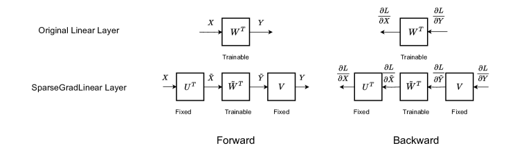
Figure 1: The first row illustrates signal propagation in the original Linear Layer, while the second row illustrates propagation with the proposed SparseGradLinear layer.

3 Method

Our aim is to reduce the amount of trainable parameters at the fine-tuning stage. Taking into account that fine-tuning data is restricted to a limited scope, we assume there is a basis where the weight gradient matrix is very close to being sparse. To identify this basis, we applied a decomposition technique to the stacked weight gradient matrices. As a result, we introduce a new PyTorch layer class, SparseGradLinear, which transitions weights to this sparse gradient space, accumulates gradients in sparse form, and enables the reverse transition back to the original space.

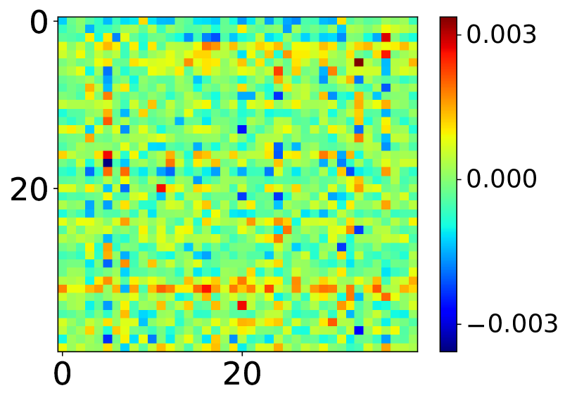
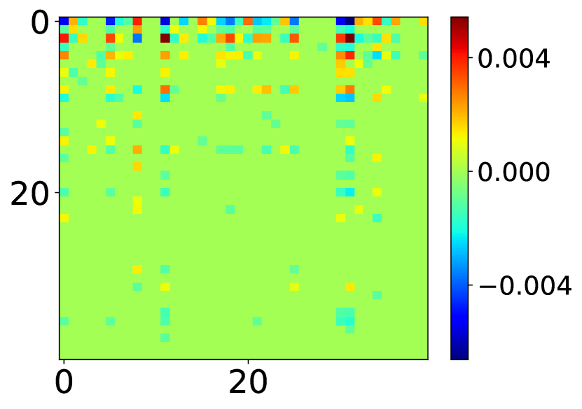
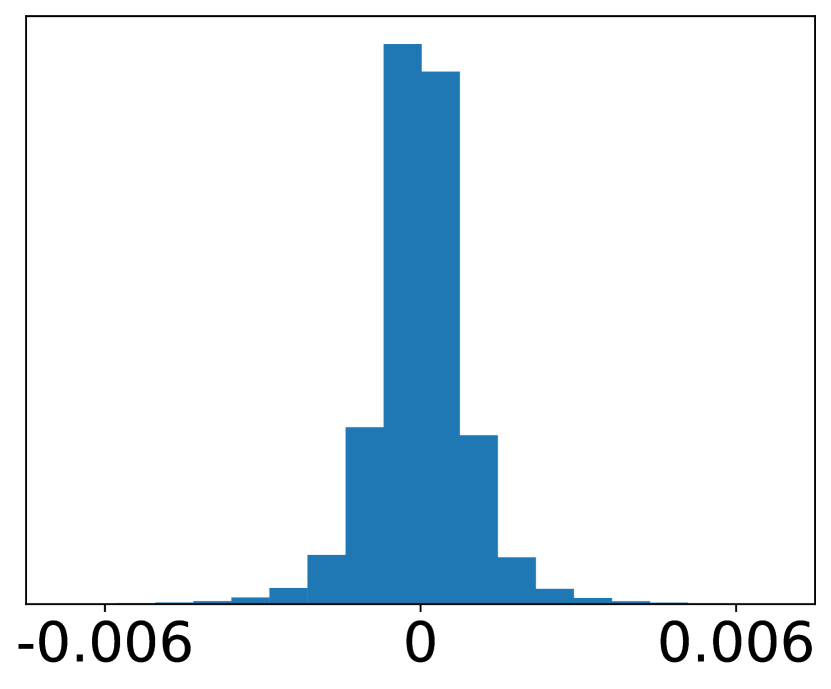
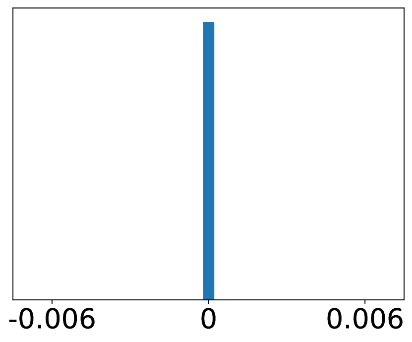
Figure 2: Gradients on the 5-th BERT MLP: $U\frac{\partial{L}}{\partial{W^{T}}}V^{T}$ (right) is more sparse than the original $\frac{\partial{L}}{\partial{W^{T}}}$ (left).

3.1 Preliminary Phase: Finding Transition Matrices

To obtain transition matrices, an initial procedure is necessary. During this, we perform $n\_steps$ of standard backpropagation by freezing the entire model and unfreezing only the linear layers in MLP blocks. We do it to obtain the set of weights gradient matrices $\frac{\partial{L}}{\partial{W}}\in\mathcal{R}^{D\_in\times D\_out}$. Stacking these matrices over $n\_blocks$ – the number of all blocks in the model – and over $n\_steps$, we obtain a 3D tensor of size $D\_in\times D\_out\times(n\_steps*n\_blocks)$.

Applying Higher Order SVD (HOSVD) Cichocki et al. (2016) to this tensor yields matrices $U\in\mathcal{R}^{D\_in\times D\_in}$, corresponding to the dimension $D\_in$ and $V^{T}\in\mathcal{R}^{D\_out\times D\_out}$, corresponding to $D\_out$. In this way, we get two orthogonal transition matrices $U,V^{T}$ which are shared across all blocks of the model. Multiplying the layer’s weight matrix on the left by $U$ and on the right by $V^{T}$ transforms it into a new space. In this transformed space, the gradient matrix exhibits greater sparsity compared to the original space. Examples of $\frac{\partial{L}}{\partial{W^{T}}}$ with and without transition to the new space are shown in Fig. 2.

3.2 Signal Propagation in SparseGradLinear Layer

Given a Transformer Linear layer with a weight matrix $W^{T}$, input activation $X$, and output $Y=XW^{T}$, we define the gradients of the output, input, and weights as $\frac{\partial{L}}{\partial{Y}}$, $\frac{\partial{L}}{\partial{X}}$, and $\frac{\partial{L}}{\partial{W^{T}}}$, respectively. To create the corresponding SparseGradLinear layer, we represent the weights in the $U,V^{T}$ basis, such that the new weights are $\tilde{W}^{T}=UW^{T}V^{T}$. Since the modules following SparseGradLinear remain unchanged in both forward and backward passes, it is crucial to maintain consistency between outputs of the Original Linear Layer $Y$ and the SparseGradLinear layer $\tilde{Y}$, as well as their input gradients $\frac{\partial{L}}{\partial{X}}$ and $\frac{\partial{L}}{\partial{\tilde{X}}}$.

Table 2 outlines these adjustments and illustrates the correspondence of variables in Torch Autograd for Linear and SparseGrad layers.

Table 2: Correspondence of variables in Torch Autograd for a regular Linear layer and SparseGradLinear.

Variable / Layer	Linear	SparseGrad
Weights	$W^{T}$	$\tilde{W}^{T}=UW^{T}V^{T}$
Input	$X$	$\tilde{X}=XU^{T}$
Output	$Y=XW^{T}$	$\tilde{Y}=XU^{T}\tilde{W}^{T}V$
Grad Output	$\frac{\partial{L}}{\partial{Y}}$	$\frac{\partial{L}}{\partial{Y}}V^{T}$
Grad Input	$\frac{\partial{L}}{\partial{X}}=\frac{\partial{L}}{\partial{Y}}W^{T}$	$\frac{\partial{L}}{\partial{\tilde{X}}}={\frac{\partial{L}}{\partial{Y}}}U^{T}\tilde{W}^{T}V$
Grad Weights	$\frac{\partial{L}}{\partial{W}}={\frac{\partial{L}}{\partial{Y}}}^{T}X$	$\frac{\partial{L}}{\partial{\tilde{W}}}=V\frac{\partial{L}}{\partial{Y}}^{T}XU^{T}$

Thus, SparseGradLinear is equivalent to 3 linear layers: first with frozen weights $U^{T}$, defined by the HOSVD, second with trainable new weights $\tilde{W}^{T}=UW^{T}V^{T}$, third with frozen weights $V$, defined by the HOSVD. A Fig. 1 shows the propagation of the signal in this structure.

3.3 Sparse-by-Dense Matrix Multiplication

We provide the SparseGradLinear class with updated Forward and Backward procedures. However, the addition of multiplications by $U,V$ into them increased the execution time and affected peak memory in the training loop.

The sparsity of the gradient tensor $\frac{\partial{L}}{\partial{\tilde{W}}}={\frac{\partial{L}}{\partial{\tilde{Y}}}}^{T}X$ results in some of the multiplicators being sparse. We explore the structure of each component in this formula and figure out that $\frac{\partial{L}}{\partial{\tilde{Y}}}$ has a sparsity approximately equal to $\frac{\partial{L}}{\partial{\tilde{W}}}$. Histograms of the percent of its non-zero elements are presented in Fig. 3. It also shows that the sparsity is "strided" - most of the rows are completely filled with zeros. These rows can be excluded from the multiplication procedure, thus optimizing it.

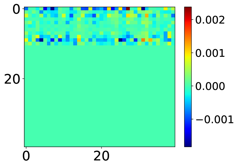
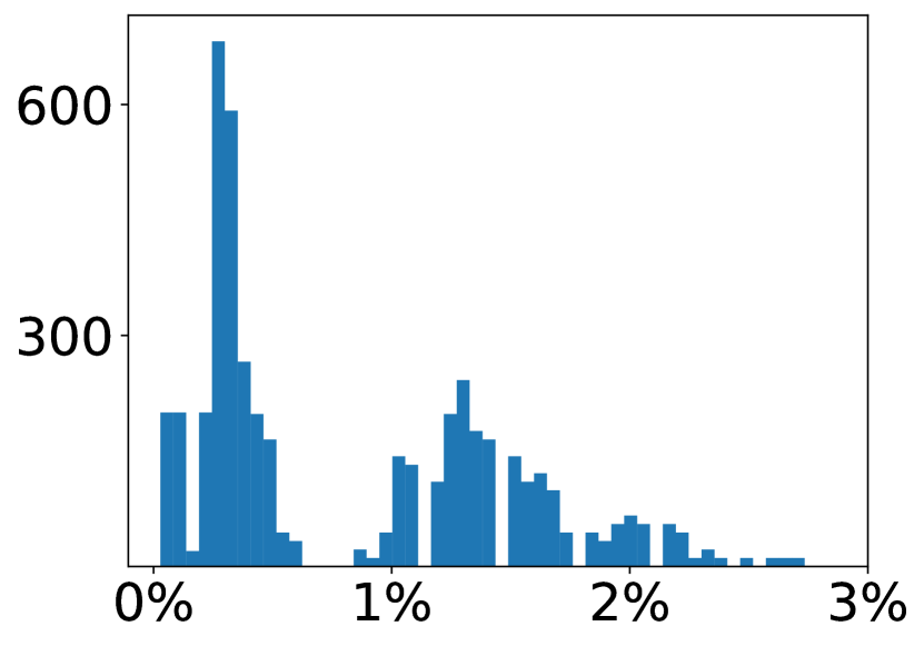
Figure 3: Strided structure of $\frac{\partial{L}}{\partial{\tilde{Y}}}$ (left) and visualizations of $\%$ nonzero elements in $\frac{\partial{L}}{\partial{\tilde{Y}}}$ throughout training (right).

More precisely, to multiply the sparse matrix $A\in\mathcal{R}^{b\times c}$ by a dense matrix $B\in\mathcal{R}^{c\times d}$ we select $rows$ and $cols$ - indices of rows and columns of $A$ which contain nonzero elements and multiply as follows:

$$C=A(rows,:)(:,cols)B(cols,:).$$ (1)

We employ $C$ either for further multiplications, or convert it into COO format and send it to SparseAdam optimizer. Indexes in COO format are defined by restoring indexes of $A$:

$$C_{coo}(rows(k),cols(l))=C(k,l).$$ (2)

As it is shown in the Table 3, such procedure significantly speeds up the harnessing of SparseGradLinear.

4 Time and Memory Consumption per Training Iteration

We measure the peak memory allocated during training using the CUDA memory allocator statistics. Table 3 demonstrates this statistic on average for all GLUE datasets for the RoBERTa_base model. The comprehensive Tables 7 and 8, which outline metrics for each dataset separately, can be found in Appendix A. Among all methods, LoRA presents the most efficient memory usage, preserving 30% of the peak memory. SparseGrad, while using slightly more memory, still achieves a 20% savings. The increase in peak memory with SparseGrad is attributed to the maintenance of matrices $U$ and $V$ and their multiplication by the dense objects, such as Input $X$.

Table 3: Training speed and memory requirements averaged on the GLUE benchmark. The last two rows of the Table 3 report the results for the SparseGrad method with Sparse-by-Dense (SD) and Regular (Reg) matrix multiplication, respectively.

Method	Steps/Sec.	Memory, MB
Regular FT	4.11	1345
LoRA	4.7	944
SparseGradSD	4.3	1016
SparseGradReg	0.9	1210

In terms of training time, LoRA demonstrates the fastest training, followed by SparseGrad, and then standard fine-tuning. Table 3 shows that Sparse-by-Dense multiplication saves approximately 12% memory, leading to an almost five-fold increase in speed.

Table 4: Comparative results of RoBERTa_large for 20-epoch task-specific fine-tuning.

Method	#Trainable params		AVG	STSB	CoLA	MNLI	MRPC	QNLI	QQP	RTE	SST2
	Model	MLP block
Regular FT	355 mln	4 mln.	85.6	91.9 $\pm.4$	67.1 $\pm 2.3$	90.8 $\pm.2$	89.9 $\pm.3$	92.9 $\pm.9$	92.3 $\pm.1$	63.9 $\pm 7.6$	96.7 $\pm.3$
LoRA	168 mln.	0.05 mln	83.7	92.1 $\pm.3$	64.4 $\pm.8$	90.7 $\pm.2$	89.9 $\pm.3$	93.2 $\pm.3$	91.8 $\pm.2$	60.2 $\pm 4.1$	96.6 $\pm.1$
SparseGrad	168 mln.	0.05 mln	85.4	92.4 $\pm.2$	63.2 $\pm 3.4$	90.7 $\pm.2$	90.5 $\pm.5$	93.3 $\pm.5$	91.7 $\pm.1$	64.7 $\pm 6.1$	96.8 $\pm.2$
MeProp	168 mln.	0.05 mln	84.3	92.3 $\pm.1$	63.7 $\pm 1.1$	90.4 $\pm.2$	89.4 $\pm.9$	92.5 $\pm.5$	91.4 $\pm.1$	59.2 $\pm 7.4$	96.2 $\pm.5$

5 Experiments

We conducted experiments on three transformer-based encoder models, BERT and RoBERTa  base and large, on the GLUE Wang et al. (2019) benchmark, and the LLaMa-2 decoder model on the OpenAssistant Conversations corpus Köpf et al. (2023). We compared the fine-tuning of the full model (Regular FT scheme) with three PEFT methods, namely LoRA, MeProp and SparseGrad, applyed to MLP blocks. To harness LoRA, we use an official repository code. For the MeProp method, we kept the largest elements in the $\frac{\partial L}{\partial W}$ matrix. The proposed SparseGrad involves replacing layers in MLP blocks with its SparseGradLinear equivalents.

5.1 Natural Language Understanding with BERT and RoBERTa

We explore the acceptable sparsity level of the gradient matrices in the “sparse” space, $\frac{\partial{L}}{\partial{\tilde{W}}}$. By varying the number of remaining parameters in the Linear Layer from $100\cdot 10^{3}$ to $18\cdot 10^{3}$, we fine-tuned the model on the GLUE benchmark and identified the point at which performance begins to degrade. This occurs when the number of trainable parameters reaches $22\times 10^{3}$, corresponding to $1\%$ of the total weights. Full experimental results can be found in Appendix C.

Guided by this heuristic, in our experiments we leave the top $1\%$ of the largest elements and set the rest to zero. To deal with SparseGradients, we use the SparseAdam optimizer - the masked version of the Adam algorithm. The remaining model parameters are trained with the standard AdamW optimizer.

We fine-tune BERT, RoBERTa_base and RoBERTa_large Zhuang et al. (2021) using Regular FT, LoRA, MeProp and SparseGrad schemes for $20$ epochs with early stopping for each task in the GLUE. We varied the batch size and learning rate using the Optuna framework Akiba et al. (2019). The learning rate ranged from $1\mathrm{e}^{-6}$ to $1{\rm e}^{-1}$, and the batch size is selected from the set {8, 16, 32}. Optimal training parameters for each task are available in the Appendix D. In LoRA we take the rank $10$ for RoBERTa_large and rank $7$ for BERT and RoBERTa_base. For SparseGrad and MeProp we keep the same number of parameters - approximately 1% of each Linear layer.

The average scores for all GLUE tasks for BERT and RoBERTa_base are in the Table 5; per-task results are placed in the Appendix B. Table 4 depicts the scores for the RoBERTa_large model. Our results indicate that SparseGrad outperforms LoRA with an equivalent number of trainable parameters across all models. For BERT, SparseGrad even exceeds the performance of Regular FT. This may be attributed to the changing basis of the weights in SparseGrad acting as a form of regularization. Concerning MeProp, it provides weaker results than SparseGrad in all cases except the RoBERTa_large on CoLA. This could be explained by the fact that our approach first transforms the elements into a special “sparse” space, while MeProp operates on gradients in the original space. In the original space, the histogram of elements is flatter (see Fig. 2), which suggests that, with the same cut-off threshold, MeProp may remove more significant elements compared to SparseGrad.

Table 5: Average scores over the GLUE benchmark for BERT and RoBERTa_base models.

Model	BERT		RoBbase
Regular FT	109 mln	82.5	125 mln	84.2
LoRA	54 mln	81.6	68 mln	83.1
SparseGrad	54 mln	82.6	68 mln	83.6
MeProp	54 mln	82.1	68 mln	82.5

5.2 Conversations with LLaMa-2

We apply the SparseGrad method to fine-tune LLaMa-2 7B Touvron et al. (2023) model on the OpenAssistant conversational dataset Köpf et al. (2023). Fine-tuning was performed on a single GPU NVIDIA A40 during 1 epoch with learning rate $9{\rm e}^{-4}$. For Regular FT, we unfroze up_proj and down_proj layers in the MLP modules with a block index divisible by 3 ($0,3,6,\dots$). We apply LoRA with rank 32 to the selected blocks, leaving the rest of the model untrainable. In the SparseGrad and MeProp methods, we also consider selected MLP modules in the transformer and leave $\approx 100,000$ (0,2%) nonzero elements in the gradient matrix. For LLaMA-2, we conducted a similar ablation study as we did for BERT and RoBERTa. We varied the number of remaining parameters in the MLP block and identified the point where the model’s performance began to decline.

We validate obtained models on the question set MT-Bench Inf from Inflection-Benchmarks Zheng et al. (2023). We followed the guidelines outlined in this work, called "Single Protocol" or "Single Answer Grading”. We got the answers by using the FastChat platform and then evaluating them using GPT-4. GPT-4 rates the answers on a scale of 1 to 10, with the evaluation prompt taken from Zheng et al. (2023).

The resulting losses and average GPT-4 scores are presented in Table 6. While the models perform similarly overall, SparseGrad slightly outperforms LoRA, MeProp, and regular fine-tuning. Examples of responses to Inflection-Benchmark samples are provided in Appendix E. These examples illustrate that, although all models produce good answers, the LoRA-trained model occasionally overlooks important nuances. In the examples given, it fails to recognize that presentations can be stressful for introverts or that hierarchy plays a significant role in Japanese corporate culture.

Table 6: Comparative results for LLaMa-2 on the OpenAssistant-1 dataset.

Method	#Train	Valid	I-Bench
	params	Loss	Score
Regular FT	22%	1.250 $\pm 0.03$	4.407
LoRA	0.5%	1.249 $\pm 0.05$	5.025
SparseGrad	0.5%	1.247 $\pm 0.03$	5.132
MeProp	0.5%	1.259 $\pm 0.04$	4.261

6 Conclusion

We propose a new selective PEFT method called SparseGrad, which identifies a space where the gradients exhibit a sparse structure and updates only its significant part. SparseGrad is validated through experiments conducted on the BERT, RoBERTa and LLaMa-2 model models, demonstrating its superiority over the additive LoRA and selective MeProp methods.

Leveraging the sparsity property significantly accelerated the calculations in SparseGrad. Our method runs faster than standard fine-tuning but slower than LoRA, while yielding better performance than LoRA; the same trend applies to memory usage. In summary, our method serves as an alternative to LoRA in situations where the performance of the final model takes precedence over the execution time. The source code as well as links to pretrained models are available at repository

7 Limitations

The main limitation of our method is the additional memory requirements during the Preliminary Phase. The extra memory is assessed as follows: we need to unfreeze the MLP layers, which hold approximately half of the training parameters in Transformers (see Table 1), store and decompose a large tensor. For instance, 30 steps in the preliminary phase result in a tensor of approximately 276 MB for BERT and ROBERTA models, and 5.2 GB for LLaMa-2.7 B models. The decomposition part can be the most memory-consuming, as it involves reshaping a 3-dimensional tensor into a matrix with a dimension size equal to the product of two dimension sizes of the tensor Cichocki et al. (2016).

However, this part is executed only once during the entire fine-tuning process and can be computed on the CPU in a short time. The Higher Order SVD decomposition of such objects takes approximately 78 seconds for BERT and RoBERTa_base layers and about 668 seconds for LLaMa on an Intel Xeon Gold 6342 CPU processor.

8 Ethics Statement

Our proposed approach involves a novel method for fine-tuning large language models, which can be considered as cost-effective as we only update $0.1\%$ of the weights. This type of fine-tuning is environmentally friendly as it reduces resource wastage. We utilized pre-trained models from the Hugging Face repository and implemented updates using the Pytorch library. We exclusively used open-source datasets to avoid any potential harm or ethical concerns. By prioritizing ethical standards and recognizing potential risks, we strive to promote responsible and sustainable research practices.

Appendix A Appendix A

Method / Dataset	AVG	STSB	CoLA	MNLI	MRPC	QNLI	QQP	RTE	SST2
Regular FT	4.11	2.9	4.3	4.2	4.1	3.1	4.7	4.2	5.1
LoRA	4.7	2.8	5.8	6.2	6.3	3.4	4.1	3.2	4.4
SparseGrad, Sparse-by-Dense	4.3	3.8	1.8	3.9	3.1	3.5	5.6	6.3	6.2
SparseGrad, Regular	0.9	0.4	0.3	0.4	1.9	0.8	0.7	1.6	1.1

Table 7: The training step execution speed, measured in steps per second (where a higher value indicates faster execution), is reported for the RoBERTa base model. The last two rows describe the SparseGradMethod with Sparse-by-Dense multiplication and with Regular matrix multiplication.

Method / Dataset	AVG	STSB	CoLA	MNLI	MRPC	QNLI	QQP	RTE	SST2
Regular FT	1345	1344	1358	1350	1362	1369	1333	1314	1339
LoRA	944	969	978	986	998	938	935	902	855
SparseGrad, Sparse-by-Dense	1016	997	1082	1017	1110	1019	981	960	980
SparseGrad, Regular	1210	1283	1212	1256	1183	1245	1172	1116	1209

Table 8: Peak memory measurement in MB for training loop for the model RoBERTa base.

Appendix B Appendix B

Table 9: Comparative results of BERT model for 20-epoch task-specific fine-tuning.

Method	#Trainable		AVG	STSB	CoLA	MNLI	MRPC	QNLI	QQP	RTE	SST2
	Parameters
	Model	MLP Layer
Regular FT	109 mln	3 mln	82.5	89.3 $\pm.6$	59.0 $\pm 1.9$	84.0 $\pm.3$	86.2 $\pm 1.1$	89.3 $\pm 1.3$	91.1 $\pm 0$	67.4 $\pm 2.8$	92.7 $\pm.1$
LoRA	53 mln	0.03 mln	81.6	89.2 $\pm.7$	58.4 $\pm 2.3$	84.2 $\pm.2$	83.8 $\pm.6$	89.3 $\pm.8$	91.0 $\pm 0$	64.6 $\pm 2.1$	92.3 $\pm.2$
SparseGrad	53 mln	0.03 mln	82.6	89.2 $\pm.4$	58.8 $\pm 0$	84.0 $\pm 1.3$	86.6 $\pm.5$	89.4 $\pm 1.6$	90.9 $\pm.3$	69.3 $\pm 2.9$	92.4 $\pm.1$
MeProp	53 mln	0.03 mln	82.1	88.9 $\pm.5$	58.4 $\pm.8$	83.3 $\pm.3$	84.2 $\pm.6$	89.6 $\pm.3$	90.4 $\pm.4$	64.9 $\pm.9$	92.1 $\pm.1$

Table 10: Comparative results of ROBERTA for 20-epoch task-specific fine-tuning.

Method	#Trainable		AVG	STSB	CoLA	MNLI	MRPC	QNLI	QQP	RTE	SST2
	parameters
	Model	MLP Layer
Regular FT	125 mln.	3 mln.	84.2	90.4 $\pm.3$	59.7 $\pm 1.4$	87.7 $\pm.1$	90.0 $\pm.6$	90.6 $\pm.8$	91.5 $\pm.1$	68.8 $\pm 2.5$	94.7 $\pm.2$
LoRA	68 mln.	0.03 mln.	83.1	90.5 $\pm.2$	60.6 $\pm 1.7$	87.5 $\pm.1$	88.4 $\pm.6$	90.0 $\pm.8$	91.4 $\pm.1$	63.1 $\pm 2.3$	94.5 $\pm.1$
SparseGrad	68 mln.	0.03 mln.	83.6	90.8 $\pm.2$	60.0 $\pm 1.6$	87.5 $\pm.1$	89.6 $\pm 1.1$	91.5 $\pm.6$	91.5 $\pm.1$	65.6 $\pm 2.1$	94.2 $\pm.1$
MeProp	68 mln.	0.03 mln.	82.5	90.7 $\pm.1$	59.2 $\pm 1.3$	85.9 $\pm.1$	89.1 $\pm 0.9$	89.4 $\pm.5$	90.5 $\pm.1$	61.5 $\pm 1.6$	94.2 $\pm.1$

Appendix C Appendix C

The average GLUE results for the BERT and RoBERTa_base models with respect to the number of remaining updated parameters in Linear layers. Tables 11, 12 shows that under the 0.8% of the remaining parameters, performance tends to decrease.

Table 11: GLUE score as a function of the weight gradient sparsity in BERT

Method	% of remained	AVG	STSB	CoLA	MNLI	MRPC	QNLI	QQP	RTE	SST2
	params
	in Linear Layers
SparseGrad	100	82.6	89.2 $\pm.4$	58.8 $\pm 0$	84.0 $\pm 1.3$	86.6 $\pm.5$	89.4 $\pm 1.6$	90.9 $\pm.3$	69.3 $\pm 2.9$	92.4 $\pm.1$
SparseGrad 18k	0.8	81.5	89.1 $\pm.3$	59.1 $\pm.5$	83.8 $\pm.1$	84.6 $\pm.8$	89.4 $\pm.8$	90.8 $\pm.2$	63.5 $\pm 5.2$	92.4 $\pm.6$
SparseGrad 22k	1	82.2	89.7 $\pm.6$	60.0 $\pm.4$	83.9 $\pm.1$	84.6 $\pm 1.5$	88.8 $\pm 1.0$	91.1 $\pm.0$	67.7 $\pm 2.5$	92.3 $\pm.3$
SparseGrad 30k	1.2	82.0	89.2 $\pm.4$	59.1 $\pm.5$	84.1 $\pm.3$	85.4 $\pm.6$	89.3 $\pm.6$	90.8 $\pm.2$	65.6 $\pm 4.6$	92.2 $\pm.4$
SparseGrad 100k	4.2	82.2	89.3 $\pm.3$	60.0 $\pm.3$	83.8 $\pm.2$	85.1 $\pm 1.2$	88.9 $\pm 1.0$	91.2 $\pm.0$	65.6 $\pm 3.3$	92.4 $\pm.3$

Table 12: GLUE score as a function of the weight gradient sparsity in ROBERTA

Method	% of remained	AVG	STSB	CoLA	MNLI	MRPC	QNLI	QQP	RTE	SST2
	params
	in Linear Layers
SparseGrad	100	83.6	90.8 $\pm.2$	60.0 $\pm 1.6$	87.5 $\pm.1$	89.6 $\pm 1.1$	91.5 $\pm.6$	91.5 $\pm.1$	65.6 $\pm 2.1$	94.2 $\pm.1$
SparseGrad 18k	0.8	83.4	90.9 $\pm.2$	59.7 $\pm.1$	87.4 $\pm.4$	89.2 $\pm.7$	89.1 $\pm.4$	91.5 $\pm.1$	60.4 $\pm 5.8$	94.0 $\pm.4$
SparseGrad 22k	1	83.6	90.6 $\pm.2$	58.8 $\pm.4$	87.7 $\pm.1$	90.0 $\pm.3$	90.1 $\pm.1$	91.3 $\pm.1$	65.5 $\pm 3.7$	94.6 $\pm.2$
SparseGrad 30k	1.2	83.6	90.8 $\pm.3$	59.4 $\pm.4$	87.6 $\pm.1$	89.8 $\pm.4$	91.0 $\pm.1$	91.3 $\pm.1$	64.9 $\pm 8.6$	94.2 $\pm.1$
SparseGrad 100k	1.4	83.9	90.9 $\pm.3$	59.8 $\pm.5$	87.0 $\pm.1$	89.7 $\pm.5$	89.6 $\pm.5$	91.4 $\pm.1$	69.4 $\pm 3.2$	94.1 $\pm.3$

Appendix D Appendix D

Best training parameters for all models. In all experiments, we repeat fine-tuning $3$ times over different seeds and report the average score.

Table 13: Best training parameters on GLUE benchmark for BERT model.

Dataset	batch size	learning rate
STSB	32	1.24e-4
CoLA	32	3.15e-5
MNLI	32	6.07e-6
MRPC	32	1.22e-5
QNLI	16	1.94e-5
QQP	32	1.41e-5
RTE	16	6.81e-5
SST2	32	1.47e-5

Table 14: Best training parameters on GLUE benchmark for RoBERTa model.

Dataset	batch size	learning rate
STSB	16	2.70e-5
CoLA	16	1.01e-5
MNLI	32	1.51e-5
MRPC	32	1.9e-5
QNLI	16	1.91e-5
QQP	16	5.11e-6
RTE	32	3.05e-5
SST2	16	1.33e-5

Table 15: Best training parameters on GLUE benchmark for RoBERTa-large model.

Dataset	batch size	learning rate
STSB	32	7.71e-5
CoLA	16	1.8e-5
MNLI	16	1.15e-6
MRPC	32	2.47e-5
QNLI	16	8.83e-6
QQP	32	7.2e-6
RTE	32	1.02e-5
SST2	32	1.02e-5

Appendix E Appendix E

Responses from the models to an example from Inflection-Benchmarks are shown. While all models perform fairly well, the LoRA-trained model overlooks the fact that public speaking can be stressful for an introvert when answering the first question.

References

- Akiba et al. (2019) Takuya Akiba, Shotaro Sano, Toshihiko Yanase, Takeru Ohta, and Masanori Koyama. 2019. Optuna: A next-generation hyperparameter optimization framework. In Proceedings of the 25th ACM SIGKDD International Conference on Knowledge Discovery & Data Mining, KDD 2019, Anchorage, AK, USA, August 4-8, 2019, pages 2623–2631. ACM.
- Cichocki et al. (2016) Andrzej Cichocki, Namgil Lee, Ivan Oseledets, Anh-Huy Phan, Qibin Zhao, and Danilo P. Mandic. 2016. Tensor networks for dimensionality reduction and large-scale optimization: Part 1 low-rank tensor decompositions. Foundations and Trends® in Machine Learning, 9(4–5):249–429.
- Devlin et al. (2019) Jacob Devlin, Ming-Wei Chang, Kenton Lee, and Kristina Toutanova. 2019. BERT: Pre-training of deep bidirectional transformers for language understanding. In Proceedings of the 2019 Conference of the North American Chapter of the Association for Computational Linguistics: Human Language Technologies, Volume 1 (Long and Short Papers), pages 4171–4186, Minneapolis, Minnesota. Association for Computational Linguistics.
- Houlsby et al. (2019) Neil Houlsby, Andrei Giurgiu, Stanislaw Jastrzebski, Bruna Morrone, Quentin De Laroussilhe, Andrea Gesmundo, Mona Attariyan, and Sylvain Gelly. 2019. Parameter-efficient transfer learning for NLP. 97:2790–2799.
- Hu et al. (2021) Edward J. Hu, Yelong Shen, Phillip Wallis, Zeyuan Allen-Zhu, Yuanzhi Li, Shean Wang, and Weizhu Chen. 2021. Lora: Low-rank adaptation of large language models. CoRR, abs/2106.09685.
- Köpf et al. (2023) Andreas Köpf, Yannic Kilcher, Dimitri von Rütte, Sotiris Anagnostidis, Zhi-Rui Tam, Keith Stevens, Abdullah Barhoum, Nguyen Minh Duc, Oliver Stanley, Richárd Nagyfi, Shahul ES, Sameer Suri, David Glushkov, Arnav Dantuluri, Andrew Maguire, Christoph Schuhmann, Huu Nguyen, and Alexander Mattick. 2023. Openassistant conversations – democratizing large language model alignment.
- Lialin et al. (2023) Vladislav Lialin, Vijeta Deshpande, and Anna Rumshisky. 2023. Scaling down to scale up: A guide to parameter-efficient fine-tuning.
- Pfeiffer et al. (2020) Jonas Pfeiffer, Andreas Rücklé, Clifton Poth, Aishwarya Kamath, Ivan Vulic, Sebastian Ruder, Kyunghyun Cho, and Iryna Gurevych. 2020. Adapterhub: A framework for adapting transformers. CoRR, abs/2007.07779.
- Sun et al. (2017) Xu Sun, Xuancheng Ren, Shuming Ma, and Houfeng Wang. 2017. meProp: Sparsified back propagation for accelerated deep learning with reduced overfitting. In Proceedings of the 34th International Conference on Machine Learning, volume 70 of Proceedings of Machine Learning Research, pages 3299–3308. PMLR.
- Touvron et al. (2023) Hugo Touvron, Thibaut Lavril, Gautier Izacard, Xavier Martinet, Marie-Anne Lachaux, Timothée Lacroix, Baptiste Rozière, Naman Goyal, Eric Hambro, Faisal Azhar, Aurelien Rodriguez, Armand Joulin, Edouard Grave, and Guillaume Lample. 2023. Llama: Open and efficient foundation language models.
- Wang et al. (2019) Alex Wang, Amanpreet Singh, Julian Michael, Felix Hill, Omer Levy, and Samuel R. Bowman. 2019. GLUE: A multi-task benchmark and analysis platform for natural language understanding. In 7th International Conference on Learning Representations, ICLR 2019, New Orleans, LA, USA, May 6-9, 2019. OpenReview.net.
- Zaken et al. (2021) Elad Ben Zaken, Shauli Ravfogel, and Yoav Goldberg. 2021. Bitfit: Simple parameter-efficient fine-tuning for transformer-based masked language-models. CoRR, abs/2106.10199.
- Zheng et al. (2023) Lianmin Zheng, Wei-Lin Chiang, Ying Sheng, Siyuan Zhuang, Zhanghao Wu, Yonghao Zhuang, Zi Lin, Zhuohan Li, Dacheng Li, Eric. P Xing, Hao Zhang, Joseph E. Gonzalez, and Ion Stoica. 2023. Judging llm-as-a-judge with mt-bench and chatbot arena.
- Zhuang et al. (2021) Liu Zhuang, Lin Wayne, Shi Ya, and Zhao Jun. 2021. A robustly optimized BERT pre-training approach with post-training. In Proceedings of the 20th Chinese National Conference on Computational Linguistics, pages 1218–1227, Huhhot, China. Chinese Information Processing Society of China.