Boundary-value problems of functional differential equations with state-dependent delays

Abstract

We prove convergence of piecewise polynomial collocation methods applied to periodic boundary value problems for functional differential equations with state-dependent delays. The state dependence of the delays leads to nonlinearities that are not locally Lipschitz continuous preventing the direct application of general abstract discretization theoretic frameworks. We employ a weaker form of differentiability, which we call mild differentiability, to prove that a locally unique solution of the functional differntial equation is approximated by the solution of the discretized problem with the expected order.

An additional difficulty is that linearizations required for solving the discretized nonlinear problem with Newton iterations are not well defined or discontinuous. We show that Newton iterations still converge if one uses the linearization in regularized solutions. The Newton iterations’ asymptotic convergence ratio is limited by the numerical discretization error. Thus, Newton iterations should show better convergence for approximations on finer meshes.

Keywords: functional differential equations, periodic solutions, boundary-value problems, collocation methods, state-dependent delay, numerical bifurcation analysis

2010 Mathematics Subject Classification: 65L03, 65L10, 65L20, 65L60

1 Introduction

Tracking time-periodic responses (periodic orbits) is a common task in numerical bifurcation analysis of nonlinear dynamical systems (Kuznetsov, 2004; Govaerts and Kuznetsov, 2007). The interest extends to periodic orbits that are dynamically unstable or extremely sensitive to parameters, as these orbits are thresholds between alternative stable states or are the link between seemingly discontinuous system responses, such as canards (Desroches et al., 2012). Dynamically unstable or sensitive orbits are beyond the reach of initial-value problem (IVP) solvers due to sensitivity to initial conditions near the periodic orbit. If the dynamical system is described by ordinary differential equations (ODEs) there are robust tools available that address sensitivity caused by dynamical instability and are able to track families of periodic orbits in one or many system parameters. Widely adopted tools for ODEs are AUTO (Doedel, 2007), MatCont (Govaerts and Kuznetsov, 2007), or coco (Dankowicz and Schilder, 2013). These tools compute solutions $y(t)\in\mathbb{R}^{n_{y}}$ of an ODE with parameters, $y^{\prime}(t)=G(y(t),p)$ with an unknown period $T$, such that $y(t)=y(t+T)$ for all $t\in\mathbb{R}$ and some unknown $T>0$. They solve the boundary-value problem (BVP) numerically with piecewise polynomial collocation similar to that described by Ascher et al. (1981), where the time-rescaled periodic orbit $t\mapsto y(t/T)$ is approximated by a piecewise polynomial $s\mapsto y^{L}(s)$ for $s\in[0,1]$ with $L$ pieces of (usually uniform) degree $m$ on $L$ subintervals of $[0,1]$. The method imposes the ODE at chosen time points (nodes) within each subinterval to construct a large nonlinear system of algebraic equations with a blockdiagonal Jacobian. Tools such as AUTO, MatCont and coco embed the BVP by including one or several parameters into the unknown and augmenting the BVP with constraints (typically affine), such as phase and pseudo-arclength conditions. This augments the blockdiagonal Jacobian, resulting in well-conditioned problems that would be ill-conditioned if a shooting approach over a bounded number of time intervals was employed instead. See (Desroches et al., 2012) for several impressive demonstrations of how to find phenomena that occur in exponentially small parameter regions in singularly perturbed problems.

Functional differential equations (FDEs)

If the right-hand side of the differential equation depends on values of $y$ at other times than the current $t$, one speaks of functional differential equations, writing

$$\dot{y}(t) =G_{\mathrm{FDE}}(y_{t},p)\mbox{,}$$ (1.1)

where the dependent variable is $y:\mathbb{R}\to\mathbb{R}^{n_{y}}$, $p\in\mathbb{R}^{n_{p}}$ are the problem parameters, and

$$G_{\mathrm{FDE}}:C^{0}([-\tau_{\max},0];\mathbb{R}^{n_{y}})\times\mathbb{R}^{n_{p}}\to\mathbb{R}^{n_{y}}$$

is a continuous nonlinear functional. We use $C^{\ell}(I;\mathbb{R}^{n})$ for the space of continuous (for $\ell=0$) or continuously differentiable (for $\ell>0$) functions from the interval $I\subset\mathbb{R}$ into $\mathbb{R}^{n}$. The subscript $t$ in $y_{t}$ denotes the time shift operator

$$C^{0}(\mathbb{R};\mathbb{R}^{n_{y}})\times\mathbb{R}\ni(y,t)\mapsto y_{t}\in C([-\tau_{\max},0];\mathbb{R}^{n_{y}})\mbox{\ with\ }y_{t}(s)=y(t+s)\mbox{}$$

(we may also simply write $\dot{y}(t)=G_{\mathrm{FDE}}(y(t+(\cdot)),p)$). Common challenging bifurcation analysis problems involving FDEs arise in optics due to transport delays (Seidel et al., 2022), in population dynamics due to non-zero maturation times (leading to implicitly defined threshold delays and integrals over the past (Gedeon et al., 2022; Diekmann et al., 2010)), or in machining due to the effects of the machining tool on the surface from the previous revolution (Insperger et al., 2008).

Collocation for FDEs

As the piecewise polynomial $y^{L}$ provides a natural interpolation the collocation methods for ODEs immediately generalize to FDEs. After time rescaling, one is looking for a $1$-periodic function satisfying the FDE

$$y^{\prime}(t)=TG_{\mathrm{FDE}}(y(t+(\cdot)/T),p),$$ (1.2)

such that one may evaluate the functional $G_{\mathrm{FDE}}$ at a collocation point $t$ using the piecewise polynomial: $(y^{L})^{\prime}(t)=TG_{\mathrm{FDE}}(y^{L}(t+(\cdot)/T),p)$. Imposition of the FDE at a time point $t\in[0,1]$ introduces coupling between values of $y$ at different times such that the Jacobian of the resulting nonlinear system of algebraic equations is no longer blockdiagonal. When one seeks to find periodic orbits one may “wrap around” when finding the value of $y$ at deviating arguments $t+s$ outside the base interval $[0,1]$ by using $(t+s)\mod 1$. So the non-diagonal coupling is the only added difficulty when formulating discretized periodic BVPs for FDEs. This motivates specialized BVP solvers and analysis for the case of finding periodic orbits in FDE problems with parameters.

Complete tools for bifurcation analysis incorporating collocation for periodic orbits were developed and implemented by Engelborghs et al. (2002) (DDE-Biftool) and Szalai (2006) (knut), see also Roose and Szalai (2007) for a review. These tools permit an arbitrary number of discrete delays as part of $G_{\mathrm{FDE}}$, which may depend on the state and system parameters (for DDE-Biftool). A-posteriori convergence tests on examples suggested convergence orders equal to the degree $m$ of the polynomial pieces for the maximum norm of the error over interval $[0,1]$. One cannot expect better (e.g., superconvergence) as the interpolation uses the piecewise polynomial $y^{L}(\cdot)$ of degree $m$ when evaluating $G_{\mathrm{FDE}}$ at the collocation points Engelborghs et al. (2001); Barton et al. (2006). Engelborghs and Doedel (2002) proved linear stability for collocation methods for time-periodic linear inhomogeneous FDEs with discrete constant delays. They pointed to “general stability theory for discretizations of nonlinear operator equations” for concluding (informally) convergence of the methods, referring to Keller (1975).

Lack of continuous differentiability of the nonlinearity

However, the argument by Engelborghs and Doedel (2002) is only valid if one treats the period $T$ of the orbit and the delays (which are system parameters) as known constants.

Let us illustrate the obstacle to applying standard arguments for convergence of numerical methods with the simple example

$$\dot{y}(t)=-y(t-p-y(t)).$$ (1.3)

This DDE fits the general form (1.1) with

$$G_{\mathrm{FDE}}(y,p)=-y(-p-y(0))\mbox{,}$$ (1.4)

which is continuous on an open subset of $C^{0}([-\tau_{\max},0];\mathbb{R})\times\mathbb{R}$ for $\tau_{\max}>\frac{\pi}{2}$ (so, $n_{y}=n_{p}=1$). The Hopf bifurcation theorem ensures that this DDE has a family of small-amplitude periodic solutions of the form $y(t)=y_{0}\sin(\theta+t/T)+O(|y_{0}|^{2})$ with $0<|y_{0}|\ll 1$ and period $T=2\pi+O(|y_{0}|^{2})$ for $p=\pi/2+O(|y_{0}|^{2})$ and arbitrary $\theta$. See (Kuznetsov, 2004) for the classical Hopf bifurcation theorem, (Hale, 1977; Diekmann et al., 1995) for the version for FDEs with constant delay, and (Sieber, 2012) for its proof for FDEs with state-dependent delays. After rescaling the time interval to $[0,1]$ the unknown period $T$ appears explicitly as a parameter such that one is looking for $1$-periodic functions $y$, periods $T$, and parameters $p$ such that

$$y^{\prime}(t)=G(y_{t},T,p)=-Ty(t-p/T-y(t)/T)\mbox{ for all $t\in[0,1)$.}$$ (1.5)

For the rescaled problem (1.5) the right-hand side nonlinearity has the form

$${G_{\mathrm{ts}}}:C^{\ell}_{\pi}\times\mathbb{R}\times\mathbb{R}\ni(y(\cdot),T,p)\mapsto Ty\left((\cdot)-p/T-y(\cdot)/T\right)\in C^{\ell}_{\pi}$$ (1.6)

where we use $C^{\ell}_{\pi}$ for spaces of $\ell$ times continuously differentiable $1$-periodic functions. We observe that unknowns appear inside the arguments of $y$, which is itself unknown, such that application of the Fréchet derivative to ${G_{\mathrm{ts}}}$ reduces the regularity of the argument $y$ of ${G_{\mathrm{ts}}}$:

$$D{G_{\mathrm{ts}}}(y,T,p)[\delta^{y},\delta^{T},\delta^{p}](t)=$$ (1.7)

$$-T\delta^{y}(t-p/T-y(t)/T)+y^{\prime}(t-p/T-y(t)/T)[\delta^{y}(t)+\delta^{p}]/T$$

$$-\delta^{T}\left[y(t-p/T-y(t)/T)+y^{\prime}(t-p/T-y(t)/T)[p+y(t)]/T\right].$$

Thus, the right-hand side ${G_{\mathrm{ts}}}$ is not differentiable or locally Lipschitz continuous if we consider it as mapping $y\in C^{\ell}_{\pi}$ into $C^{\ell}_{\pi}$ for any $\ell\geq 0$. The review by Hartung et al. (2006) pointed out this lack of continuous differentiability and its consequences (see also Cassidy et al. (2019)). For example, solutions for IVPs are not unique if one permits $C^{0}$ initial conditions. If the initial conditions are at least $C^{1}$ and compatible Walther (2003), then the dependence of IVP solutions on initial values is $C^{1}$ but results on higher regularity are missing. Large parts of the theory for FDEs as developed in textbooks by Hale (1977), Hale and Verduyn Lunel (1993) and Diekmann et al. (1995) relies strongly on continuous differentiability of ${G_{\mathrm{ts}}}$ acting on arguments $y\in C^{0}$, and are, thus, not applicable to problems such as (1.3).

Convergence of numerical discretization methods for BVPs

Similarly, discretization theory for boundary-value problems (BVPs) has been developed for nonlinearities ${G_{\mathrm{ts}}}$ that are Fréchet differentiable for $C^{0}$ arguments by Maset (2015b, a, 2016). Andò and Breda (2020) noted that for periodic BVPs with unknown period $T$ the rescaling by the unknown period $T$ introduces a state dependence of the deviating time arguments (namely on $T$, see the term $Ty(t-p/T\ldots)$ in (1.5)), even for FDE problems with constant delay. This causes a loss of differentiability of the problem’s nonlinearity with respect to the unknown $T$. Careful reanalysis of the general framework constructed by Maset (2016) showed that continuous differentiability with respect to the scalar variable $T$ is only needed in a single point, namely the assumed-to-exist solution of the BVP. Thus, Andò and Breda (2020) proved convergence of the routinely used methods in DDE-Biftool and knut for FDEs with constant delays, closing the gap left in the argument of Engelborghs and Doedel (2002).

The analysis of Andò and Breda (2020) leaves the question open how necessary special treatment of the unknown period $T$ is (a finite-dimensional part of the unknowns of the problem), or if convergence of numerical discretization for periodic BVPs can be proved without assuming Fréchet differentiability of the right-hand side. The review by Hartung et al. (2006) points to the appropriate generalized differentiability properties that are satisfied by the nonlinearities occuring in FDEs. As one can see in the right-hand side (1.6) of example (1.5) and its derivative (1.7), nonlinearities in FDEs are Fréchet differentiable $\ell$ times with respect to their arguments $y$ and $p$ only if $y\in C^{\ell}$. In (1.7) we also see that, while the derivative depends on $y^{\prime}$, it does not depend on $(\delta^{y})^{\prime}$. We use this property of restricted differentiability (we call it mild in Definition 2.1) to prove our central convergence result for discretizations of embedded periodic BVPs of FDEs.

Feasibility and convergence of Newton iterations

We also address an issue left open by Andò and Breda (2020), even for the case of constant delays. Since the $y$-component of a numerical approximation $(y(\cdot),T,p)$ is not differentiable for typical polynomial collocation schemes, but only in $C^{0,1}_{\pi}$ (the space of Lipschitz continuous $1$-periodic functions), it is unclear how the derivative of the right-hand side can be evaluated safely in approximate solutions during Newton iterations, as it requires evaluation of $y^{\prime}(t)$ at a difficult-to-control number of times $t$. In the best-case scenario the Jacobian of the discretized problem will depend discontinuously on the solution such that the standard convergence argument for Newton iterations needs to be revisited for FDEs. We will formulate the Newton iteration with a regularized Fréchet derivative with a smoothing parameter $\rho$. For the types of nonlinearitiy admissible in typical software tools the smoothing parameter $\rho$ can be set to $0$, resulting in Fréchet derivatives that are discontinuous in $(y^{L},T,p)$.

We will state the main results and their assumptions in section 2. Within section 2 we will also point forward to sections 3–7 where equivalent formulations and proofs of the main results are presented. Section 8 describes the class of problems treatable with DDE-Biftool, and performs a few numerical tests on the illustrative example (1.3).

2 Main results

2.1 Periodic BVPs for FDEs and mild differentiability

Consider an embedded periodic BVP of the form

$$y^{\prime}(t) =TG_{\mathrm{FDE}}(y(t+(\cdot)/T),p), 0 =R_{\mathrm{aff}}[y,T,p]\mbox{,}$$ (2.1)

for continuous $1$-periodic $y:\mathbb{R}\to R^{n_{y}}$, period $T$, and parameter $p\in\mathbb{R}^{n_{p}}$, where $G_{\mathrm{FDE}}:C^{0}([-\tau_{\max},0];\mathbb{R}^{n_{y}})\times\mathbb{R}^{n_{p}}\to\mathbb{R}^{n_{y}}$ is continuous. The affine map $R_{\mathrm{aff}}:C^{0}_{\pi}\times\mathbb{R}^{n_{p}+1}\to\mathbb{R}^{n_{p}+1}$ defines constraints, making the system “square” when including the parameters $T$ and $p$ as unknowns ($C^{k}_{\pi}$ are $C^{k}$ spaces of $1$-periodic functions). The constraints should also eliminate the shift symmetry that $y(\theta+(\cdot))$ is a solution of (1.3) for all $\theta$ whenever it is a solution for $\theta=0$.

Nonlinearities such as $G_{\mathrm{FDE}}$ require the concept of mild differentiability to describe their regularity.

Definition 2.1 (Mild differentiability).

A functional $G:C^{0}\to\mathbb{R}^{n_{G}}$ is called ${\ell_{\max}}$ times mildly differentiable if

1. (restricted continuous differentiablity) $G|_{C^{\ell}}$ is $\ell$ times differentiable for $\ell\leq{\ell_{\max}}$ (in particular, $G$ is continuous), and

2. (extendability) the map $C^{\ell}\times C^{\ell}\ni(u,\delta^{u})\mapsto D^{\ell}G(u)(\delta^{u})^{\ell}\in\mathbb{R}^{n_{G}}$ has a continuous extension to $C^{\ell}\times C^{\ell-1}$ for all $\ell\leq{\ell_{\max}}$.

This definition extends naturally to the functional on the right-hand side of (2.1),

$$G(y,T,p):=TG_{\mathrm{FDE}}(y(t+(\cdot)/T),p),$$

through the embedding of $\mathbb{R}^{n_{p}+1}$ into $C^{0}_{\pi}$ that treats a vector $(T,p)$ as the constant function $t\mapsto(T,p)$. The nonlinearity $(y,T,p)\mapsto-Ty(-p/T-y(0)/T)$ used in example (1.5) is an example of a functional that is mildly differentiable to arbitrary degree.

Assumption 2.2 (Assumptions on the BVP).

1. (Mild differentiability) The right-hand side $G_{\mathrm{FDE}}$ in the DDE (2.1) is mildly differentiable to order ${\ell_{\max}}\geq 1$.

2. (Existence of solution) BVP (2.1) has a solution $(y^{*},T^{*},p^{*})$.

3. (Linear well-posedness) The BVP (2.1), linearized in $(y^{*},T^{*},p^{*})$, has only the trivial solution $(\delta^{y},\delta^{T},\delta^{p})=0$.

Corollary 5.3 below shows that points 1 and 2 imply that $y^{*}\in C^{2}_{\pi}$ such that the derivative $DG(y^{*},T^{*},p^{*})$ exists for the mildly differentiable $G$, which permits us to pose Assumption 2.2, point 3. Section 5 will restate Assumption 2.2 for a fixed-point problem equivalent to (2.1), defined later in (3.6).

2.2 Convergence of solution of discretized BVP

For polynomial collocation the unknown function is a $1$-periodic continuous piecewise polynomial $y^{L}$ on a mesh given as $0=t_{0}<\ldots<t_{L}=1$. More precisely, $y^{L}$ is a polynomial of degree $m$ on $[t_{i-1},t_{i}]$ for all $i=1,\ldots,L$ in each of its $n_{y}$ components, $y^{L}$ is continuous, and $y(t)=y(t+1)$ for all $t$. Additional unknowns are the parameters $(T^{L},p^{L})$, resulting in $n_{y}mL+n_{p}+1$ unknowns overall. The system of algebraic equations,

$$0 =(y^{L})^{\prime}(t_{i,j})-T^{L}G_{\mathrm{FDE}}(y^{L}(t_{i,j}+(\cdot)/T^{L}),p^{L}), 0 =R_{\mathrm{aff}}[y^{L},T^{L},p^{L}]$$ (2.2)

for $1\leq i\leq L$, $1\leq j\leq m$, evaluates the FDE at the collocation points $t_{i,j}=t_{i-1}+(t_{i}-t_{i-1})t_{\mathrm{c},j}$, where the points $t_{\mathrm{c},j}$ are the $m$ collocation points for degree $m-1$ on the interval $[0,1]$ for a sequence of orthogonal polynomials (e.g. of Gauss-Legendre or Chebyshev type). The strategy for adjusting approximation quality is a finite-element approach Andò and Breda (2020); Andò (2020), keeping the degree $m$ bounded, and considering the limit $L\to\infty$, refining the mesh such that

$$\max\{t_{i}-t_{i-1}\}\leq C_{\mathrm{msh}}/L$$ (2.3)

for a bounded $C_{\mathrm{msh}}$ independent of $L$. In contrast, the strategy of keeping $L$ bounded and letting $m$ go to infinity is called the spectral element method in (Breda et al., 2005; Trefethen, 1996). Spectral methods promise exponential convergence, but require bounds on all derivatives of $y^{*}$. In the proofs of Lemmas 6.1 and 6.5 we rely on the boundedness of the degree $m$, but both Lemmas only require $G$ to be mildly differentiable once.

We can now state the following convergence theorem for the discretized BVP (2.2).

Theorem 2.3 (Convergence of discretization).

Under Assumption 2.2 the discretized BVP (2.2) with (2.3) has a locally unique solution $x_{L}=(y^{L},T^{L},p^{L})$ near $x^{*}=(y^{*},T^{*},p^{*})$ for all sufficiently large $L$. The solution satisfies

$$\|x_{L}-x^{*}\|_{0,1}:=\max\{\|y^{L}-y^{*}\|_{0,1},|T^{L}-T^{*}|,|p^{L}-p^{*}|\}=O\left(L^{-\min\{{\ell_{\max}},m\}}\right),$$ (2.4)

The norm $\|y^{L}-y^{*}\|_{0,1}$ in (2.4) is the Lipschitz norm of the discretization error.

Proof through equivalent fixed-point problem

Andò (2020); Andò and Breda (2020) reformulate the BVP (2.1) as a fixed-point problem, following the general framework of Maset (2016). We modify this approach in section 3 to exploit the special structure present in periodic BVPs by constructing a fixed-point problem where the right-hand side is compact and maps spaces of periodic functions into spaces of periodic functions.

For this fixed-point problem the discretization corresponds to inserting a projection operator $\mathcal{P}_{L}$ onto the space of discontinuous piecewise polynomials of degree $m-1$ in between the nonlinearity and the integral operator. This formulation ensures that the space of numerical solutions $y^{L}$ consists of continuous $1$-periodic piecewise polynomials of degree $m$. Theorem 6.6 in section 6 establishes convergence for the discretized fixed-point problem.

We introduce basic properties of mildly differentiable functionals in Section 4, such as validity of the chain rule, which ensures that $t\mapsto TG_{\mathrm{FDE}}(y(t+(\cdot)/T,p)$ is in $C^{\ell}$ if $y\in C^{\ell}$ and $G_{\mathrm{FDE}}$ is $\ell$ times mildly differentiable. Mild differentiability of $G_{\mathrm{FDE}}$ helps us in section 6 to establish consistence and stability of the numerical method and the smallness of the nonlinear terms, leading to the proof of Theorem 6.6 and, thus, Theorem 2.3.

2.3 Convergence of Newton iteration

As the numerical approximations $y^{L}$ are not differentiable, the Newton iteration cannot evaluate the Fréchet derivative $DG_{\mathrm{FDE}}$ in numerical approximations $(y^{L}(t_{i,j}+(\cdot)/T^{L}),p^{L})$. Thus, we can only apply derivatives in a regularized numerical solution. Denoting the right-hand side of the nonlinear algebraic system (2.2) as $F_{L}(x_{L})$ with $x_{L}=(y^{L},T^{L},p^{L})$, we consider the iteration (with iterates denoted by superscripts)

$$x_{L}^{k+1} =x_{L}^{k}-\left[DF_{L}(S_{\rho}x_{L}^{k})\right]^{-1}F_{L}(x_{L}^{k}),$$ (2.5)

where $\rho\geq 0$ is small and $S_{\rho}:C^{0,1}_{\pi}\to C^{1,1}_{\pi}$ and $L^{\infty}_{\pi}\to C^{0,1}_{\pi}$ is a smoothing operator satisfying the approximation property

$$\|S_{\rho}u-v\|_{0} \leq\|u-v\|_{\infty}\hskip 4.30554pt+\rho\|v\|_{0,1} u\in L^{\infty}_{\pi} v\in C^{0,1}_{\pi}$$ for , , (2.6)

$$\|S_{\rho}u-v\|_{1} \leq\|u-v\|_{0,1}\ +\rho\|v\|_{1,1} u\in C^{0,1}_{\pi} v\in C^{1,1}_{\pi}$$ for , .

In (2.6) we use the notations $L^{\infty}_{\pi}$ and $C^{k,1}_{\pi}$ for $1$-periodic functions that are essentially bounded or $C^{k}$ with Lipschitz continuous $k$-th derivative, with their respective norms. The smoothing operation is only applied to the $y$-component of $x_{L}^{k}$. An example of a smoothing operator $[S_{\rho}y](t)$ satisfying (2.6) is the averaging of $y$ over a window of length $\rho$ around $t$, as discussed in Section 7.2. For the regularized Newton iteration we prove the following.

Lemma 2.4 (Convergence of regularized Newton iteration).

There exists a monotone increasing continuous function $\omega:[0,\infty)\to[0,\infty)$ with $\omega(0)=0$ such that, for sufficiently large $L$ and with initial guess $x_{L}^{0}$ sufficiently close to $x^{*}=(y^{*},T^{*},p^{*})$, the iteration distance $\delta^{k}_{L}=x^{k}_{L}-x^{\infty}_{L}$ satisfies

$$\frac{\|\delta^{k+1}_{L}\|_{0,1}}{\|\delta^{k}_{L}\|_{0,1}}\leq\omega(\|\delta^{k}_{L}\|_{0,1}+2\|\delta^{\infty}_{L}\|_{0,1})+\omega(\rho\|x^{*}\|_{1,1}+\|\delta^{k}_{L}\|_{0,1}+\|\delta^{\infty}_{L}\|_{0,1})$$ (2.7)

In (2.7) the norm subscript $\|\cdot\|_{k,j}$ of $x$ ($x^{*}$, $x_{L}^{k}$, $x_{L}^{\infty}$, respectively) equals the norm subscript of its $y$ component. The quantity $\delta_{L}^{\infty}=x_{L}^{\infty}-x^{*}$ is the discretization error estimated in Theorem 2.3. To achieve a limited form of quadratic convergence of the Newton iteration it is not sufficient to require mild differentiability of $G_{\mathrm{FDE}}$ to order ${\ell_{\max}}=2$. Instead, in addition to mild differentiability the derivative of the right-hand side $DG_{\mathrm{FDE}}$ has to satisfy an extended local Lipschitz condition. This condition requires that there exists a $C_{\mathrm{eL}}>0$ such that

$$|DG_{\mathrm{FDE}}(y_{t}^{*}+z^{1}_{t},p^{*}+q^{1})[z^{2}_{t},q^{2}]-DG_{\mathrm{FDE}}(y_{t}^{*},p^{*})[z^{2}_{t},q^{2}]|\leq\\ C_{\mathrm{eL}}\max\{\|z^{1}\|_{1},|q^{1}|\}\max\{\|z^{2}\|_{1},|q^{2}|\}$$ (2.8)

for sufficiently small $\|z^{1}\|$, $|q^{1}|$ and all $t\in[0,1]$. If $DG_{\mathrm{FDE}}$ satisfies (2.8) then the function $\omega$ in Lemma 2.4 satisfies $\omega(s)\leq C_{\mathrm{eL}}\cdot s$, such that the Newton iteration converges approximately quadratically:

$$\frac{\|\delta^{k+1}_{L}\|_{0,1}}{\|\delta^{k}_{L}\|_{0,1}}\leq C\left[\|\delta^{k}_{L}\|_{0,1}+\|\delta^{\infty}_{L}\|_{0,1}+\rho\|x^{*}\|_{1,1}\right]\mbox{\quad for some $C>0$.}$$ (2.9)

As we will explain in section 7.3, the extended local Lipschitz condition (2.8) does not follow from second-order mild differentiability, such that it needs to be imposed as a separate assumption (in contrast to classical continuous differentiability).

For right-hand sides $G_{\mathrm{FDE}}$ that are admissible for numerical software tools such as DDE-Biftool and knut the limit $\rho\to 0$ of the smoothing operator $S_{\rho}$ exists (and is used in the implementation). Furthermore, the admissible nonlinearities $G$ satisfy the extended local Lipschitz condition (2.8) whenever the coefficients entered by the user (right-hand sides and discrete delays) are at least $C^{2}$ in their arguments. In this case the convergence ratio of the Newton iteration is approximately quadratic but limited from below by the discretization error $\|\delta_{L}^{\infty}\|_{0,1}$.

2.4 Illustrative example of BVP

We will use the example (1.3) throughout to illustrate concepts and results. The embedded BVP for finding periodic orbits of this FDE, rescaled to base interval $[0,1]$ with a possible choice for additional affine conditions is

$$y^{\prime}(t) =-Ty(t-(p+y(t))/T),\mbox{\quad($y(t)=y(t+1)$ for all $t\in\mathbb{R}$),}$$ (2.10)

$$0 =R_{\mathrm{aff}}[y,T,p]:=\begin{bmatrix}y(0)\\ 2\int_{0}^{1}\sin(2\pi t)y(t)\mathop{}\!\mathrm{d}t-y_{0}\end{bmatrix}$$ (2.11)

for a range of small $y_{0}$. It is sufficient to impose (2.10) on the base interval $[0,1)$, if one takes into account the periodicity of $y$. For the choice (2.11) of $R_{\mathrm{aff}}$ the first condition fixes the phase of the solution $y$ (serving as a phase condition) and the second condition fixes the amplitude, locally parametrizing the solution family by the constant $y_{0}$ (thus, serving as a pseudo-arclength condition). System (2.10)–(2.11) will have solutions of the form $y(t)=y_{0}\sin(2\pi t)+O(|y_{0}|^{2})$, $T=2\pi+O(|y_{0}|^{2})$, $p=\pi/2+O(|y_{0}|^{2})$ for small $y_{0}$ according to the Hopf bifurcation theorem Sieber (2012). The unknowns in this problem are $(y(\cdot),T,p)$.

The functional $G(y,T,p)$ for this example and its derivative (defined on $C^{1}_{\pi}\times\mathbb{R}^{2})$) have already been used for illustration in (1.5) and in (1.7).

3 Fixed-point problem equivalent to periodic BVP and relevant notation

In the formulation (2.1) the unknown period $T$ plays the same role as a problem parameter. Thus, in the following we collect $T$ and $p$ into a $(n_{p}+1)$-dimensional parameter vector $\mu=(T,p)$, introducing the nonlinear functional

$$G(y,\mu) =TG_{\mathrm{FDE}}(y((\cdot)/T),p)\mbox{,\quad where now $\mu=(T,p)\in\mathbb{R}^{n_{\mu}}$, $n_{\mu}=n_{p}+1$,}$$ (3.1)

and abbreviate $R_{\mathrm{aff}}[y,\mu]=R_{\mathrm{aff}}[y,T,p]$ to simplify notation. Thus (2.1) is a special case of the general BVP

$$\begin{aligned} y^{\prime}(t)&=G(y_{t},\mu),&&\in\mathbb{R}^{n_{y}}\mbox{\ for $t\in[0,1)$,}&&\mbox{(FDE for $1$-periodic continuous $y$),}\\ 0&=R_{\mathrm{aff}}[y,\mu]&&\in\mathbb{R}^{n_{\mu}}&&\mbox{(affine constraints).}\end{aligned}$$ (3.2)

We reformulate (3.2) as fixed-point problem for the solution, obtained from the differential equation through the variation-of-constants formula, following (Andò and Breda, 2020),

$$y(t) =y(0)+\int_{0}^{t}G(y_{s},\mu)\mathop{}\!\mathrm{d}s.$$ (3.3)

We plan to pose the fixed-point problem in a space of periodic functions of period $1$. However, the right-hand side of equation (3.3) is not guaranteed to be $1$-periodic even if $y$ is $1$-periodic. To enforce period $1$, we subtract the average of the integrand and then impose that this average is zero as a separate equation, replacing the periodic boundary condition. We also introduce the new variable $\alpha\in\mathbb{R}^{n_{y}}$, which will be equal $y(0)$ in the solution. Hence, BVP (2.1) is equivalent to the system

$$y(t) =\alpha+\int_{0}^{t}G(y_{s},\mu)\mathop{}\!\mathrm{d}s-t\int_{0}^{1}G(y_{s},\mu)\mathop{}\!\mathrm{d}s, \in\mathbb{R}^{n_{y}}\mbox{\ for $t\in[0,1]$,}$$

$$0 =\int_{0}^{1}G(y_{s},\mu)\mathop{}\!\mathrm{d}s, \in\mathbb{R}^{n_{y}},$$ (3.4)

$$0 =R_{\mathrm{aff}}[y,\mu] \in\mathbb{R}^{n_{\mu}}$$

for the variables $y$, which is a continuous $1$-periodic function with $y(t)\in\mathbb{R}^{n_{y}}$, the initial value $\alpha\in\mathbb{R}^{n_{y}}$ and the vector of system parameters $\mu\in\mathbb{R}^{n_{\mu}}$ (where $\mu=(T,p)$ such that $\mu$ also includes the unknown period $T$).

The subtraction of the integrand’s average and replacement of periodic boundary conditions by a condition stating that this average is zero modifies the fixed-point problems considered by Andò and Breda (2020). The first, infinite-dimensional, component of (3.4) is already in the form of a fixed-point problem. The other two components can be modified to become fixed point problems for the operator

$$\Phi(x):=\begin{bmatrix}t\mapsto\alpha+\displaystyle\int_{0}^{t}G(v_{s},\mu)\mathop{}\!\mathrm{d}s-t\int_{0}^{1}G(v_{s},\mu)\mathop{}\!\mathrm{d}s\\[4.30554pt] \alpha+\displaystyle\int_{0}^{1}G(v_{s},\mu)\mathop{}\!\mathrm{d}s\\[4.30554pt] \mu+R_{\mathrm{aff}}[v,\mu]\end{bmatrix}\mbox{\quad for $x=(v,\alpha,\mu)$}$$ (3.5)

where $v$ is $1$-periodic with $v(t)\in\mathbb{R}^{n_{y}}$, $\alpha\in\mathbb{R}^{n_{y}}$, $\mu\in\mathbb{R}^{n_{\mu}}$. The fixed-point problem

$$x=\Phi(x)$$ (3.6)

is then equivalent to the original problem of finding a periodic solution of FDE (1.1) in the sense that for every periodic solution $y(t)$ with period $T>0$ of (1.1) at parameter $p$, there exists a phase shift $\theta\in\mathbb{R}$ such that $x=(t\mapsto y(\theta+tT),y(\theta),T,p)$ is a solution of (3.6), and, vice versa, for a fixed point $x=(v,\alpha,\mu)=(v,\alpha,T,p)$ of $\Phi$ the function $y(t)=v(t/T)$ is a periodic solution of (1.1) with period $T$ at parameter $p$, $\alpha$ must be equal to $v(0)$, and $(v,T,p)$ satisfy the constraints $R_{\mathrm{aff}}[v,T,p]$.

Notation for function spaces and norms

The definition of $\Phi$ in (3.5) had not specified the function space for the $v$ component of $x$ yet as we have not discussed what type of perturbation a discretization may introduce for $\Phi$. To specify suitable spaces we use the notation

$$C^{k\phantom{,1}}_{\pi} \!=\{v:\mbox{\ $k\times$\,cont.\,diff.,\,}v(t)=v(t+1)\mbox{\ for all $t$}\}, \|v\|_{k\phantom{,1}} \!=\max_{t\in[0,1],j\leq k}|v^{(j)}(t)|,$$

$$C^{k,1}_{\pi} =\{v\in C^{k}_{\pi},\operatorname{Lip}v^{(k)}<\infty\}, \|y\|_{k,1} \!=\max\{\|v\|_{k},\operatorname{Lip}v^{(k)}\},$$

$$L^{\infty}_{\pi} =\{y\mbox{\ ess.bd.,\ }v(t)=v(t+1)\mbox{\ for all $t$}\}, \|v\|_{\infty}\ =\operatorname{ess\,sup}_{t\in[0,1]}|v(t)|.$$

The dimension of the function’s value $v(t)$ is determined by context such that we often drop domain and codomain indicators in the spaces. Otherwise we write, e.g., $C^{k,j}_{\pi}(\mathbb{R}^{n_{u}})$ or $L^{\infty}_{\pi}(\mathbb{R}^{n_{u}})$.

Linear and nonlinear part of fixed-point problem $x=\Phi(x)$

The variable $x$ has several components, $x=(v,\alpha,\mu)$, introduced above, of which only the first one, $v$, is infinite-dimensional such that all norms of spaces for $v$ can be trivially extended by the finite-dimensional maximum norms of $\alpha$ and $\mu$. Hence, we define the extended spaces

$$C^{k,j}_{\mathrm{e}} =C^{k,j}_{\pi}\times\mathbb{R}^{n_{y}}\times\mathbb{R}^{n_{\mu}}, L^{\infty}_{\mathrm{e}} =L^{\infty}_{\pi}\times\mathbb{R}^{n_{y}}\times\mathbb{R}^{n_{\mu}},$$

and continue to use the $\|\cdot\|_{k,j}$ or $\|_{\cdot}\|_{\infty}$ notation for their respective norms. We split the operator $\Phi$, defined in (3.5), into a compact linear part $\mathcal{L}$ and a nonlinear part $g$, such that $\Phi=\mathcal{L}\circ g$. For $\mathcal{L}$ and $g$ we can now pick specific spaces:

$$g :C^{0,1}_{\mathrm{e}}\to C^{0}_{\mathrm{e}}\mbox{,\quad with} g\left(\begin{bmatrix}v\\ \alpha\\ \mu\end{bmatrix}\right) =\begin{bmatrix}t\mapsto G(v_{t},\mu)\\ \alpha\\ \mu+R_{\mathrm{aff}}[v,\mu]\end{bmatrix}\mbox{,\quad and}$$ (3.7)

$$\mathcal{L} :\begin{aligned} &L^{\infty}_{\mathrm{e}}\to C^{0,1}_{\mathrm{e}}\\ \makebox[0.0pt]{or\qquad}&C^{\ell}_{\mathrm{e}}\to C^{\ell+1}_{\mathrm{e}}\end{aligned}\mbox{,\quad with} \mathcal{L}\begin{bmatrix}w\\ \alpha\\ \nu\end{bmatrix}\hskip 8.00003pt =\begin{bmatrix}\displaystyle t\mapsto\alpha+\int_{0}^{t}w(s)\mathop{}\!\mathrm{d}s-t\int_{0}^{1}w(s)\mathop{}\!\mathrm{d}s\\[5.69054pt] \alpha+\displaystyle\int_{0}^{1}w(s)\mathop{}\!\mathrm{d}s\\ \nu\end{bmatrix}.$$ (3.8)

Our main convergence theorem for the fixed-point problem, Theorem 6.6, proves that the fixed point $x^{L}$ of a discretized operator $\Phi_{L}$ converges with the rate expected by the order of the discretization scheme to a fixed point $x^{*}$ of $\Phi$ under appropriate conditions. This convergence will operate on a small ball $B^{0,1}_{r}(x^{*})$ of Lipschitz continuous functions in $C^{0,1}_{\mathrm{e}}$ around $x^{*}$. The center $x^{*}$ has higher-order regularity than $C^{0,1}_{\mathrm{e}}$: $x^{*}\in C^{{\ell_{\max}}+1}_{\mathrm{e}}$, where ${\ell_{\max}}\geq 0$ depends on regularity assumptions on the right-hand side $G$.

Discretized fixed-point problem

For functions $z\in C^{0}_{\pi}$ we define the interpolation projection $P_{L}z$ as the unique piecewise polynomial on mesh $(t_{i})_{i=0}^{L}$ of degree $m-1$ where the piece on each interval $(t_{i-1},t_{i})$ equals $z$ on the nodes $t_{i,j}$:

$$P_{L}: \phantom{=\ }C^{0}_{\pi}\mapsto L^{\infty}_{\pi},$$

$$P_{L}z =\hat{z}\quad\begin{aligned} &\mbox{with $\hat{z}(t_{i,j})=z(t_{i,j})$ for all $i\in\{1,\ldots,L\},j\in\{1,\ldots,m\}$,}\\ &\mbox{and\ $\hat{z}$ is degree $m-1$ polynomial on $(t_{i-1},t_{i})$ for all $i\in\{1,\ldots,L\}$.}\end{aligned}$$

In the name $P_{L}$ we do not indicate the dependence on the interpolation degree $m-1$ as we will keep this degree constant, studying only the limit $L\to\infty$ in our convergence analysis. The dependence on the mesh $(t_{i})$, which will change with increasing $L$, is also implicitly included in the subscript $L$. The interpolating piecewise polynomial $t\mapsto[P_{L}z](t)$ is not necessarily continuous as it may have discontinuities at the mesh boundaries $t_{i}$, such that the codomain of $P_{L}$ is $L^{\infty}_{\pi}$.

Lemma 3.1 (Equivalence of discretized fixed point problem).

The discretized BVP (2.2) is equivalent to the fixed point problem

$$x =\mathcal{L}\mathcal{P}_{L}g(x)=:\Phi_{L}(x),$$ (3.9)

where $\mathcal{L}:L^{\infty}_{\mathrm{e}}\to C^{0,1}_{\mathrm{e}}$ and $g:C^{0,1}_{\mathrm{e}}\to C^{0}_{\mathrm{e}}$ are defined in (3.7) and (3.8), and $\mathcal{P}_{L}$ is the trivial extension of $P_{L}$,

$$\mathcal{P}_{L}:C^{0}_{\mathrm{e}}\to L^{\infty}_{\mathrm{e}},\qquad\mathcal{P}_{L}\begin{bmatrix}w\\ \alpha\\ \nu\end{bmatrix}=\begin{bmatrix}P_{L}w\\ \alpha\\ \nu\end{bmatrix}.$$ (3.10)

Proof.

For arbitrary $y\in C^{0}_{\pi}$ and $\mu\in\mathbb{R}^{n_{\mu}}$, let us denote by ${G_{\mathrm{ts}}}(y,\mu)$ the function $s\mapsto G(y_{s},\mu)$. With this notation, the fixed-point problem $x=\mathcal{L}\mathcal{P}_{L}g(x)$ is equivalent to (calling the components of $x=(v,\alpha,\mu)$)

$$v(t) =\alpha+\int_{0}^{t}[P_{L}{G_{\mathrm{ts}}}(v,\mu)](s)\mathop{}\!\mathrm{d}s-t\int_{0}^{1}[P_{L}{G_{\mathrm{ts}}}(v,\mu)](s)\mathop{}\!\mathrm{d}s$$

$$0 =\int_{0}^{1}[P_{L}{G_{\mathrm{ts}}}(v,\mu)](s)\mathop{}\!\mathrm{d}s$$ (3.11)

$$0 =R_{\mathrm{aff}}[v,\mu].$$ (3.12)

For arbitrary $(y^{L},\mu)$ the system of collocation equations $(y^{L})^{\prime}(t_{i,j})=G(y^{L}_{t_{i,j}},\mu)$ for $i=1,\ldots,L$, $j=1,\ldots,m$ is equivalent to the identity

$$y^{L}(t)=y^{L}(0)+\int_{0}^{t}\left[P_{L}{G_{\mathrm{ts}}}(y^{L},\mu)\right](s)\mathop{}\!\mathrm{d}s$$ (3.13)

for the piecewise polynomial $y^{L}$ by construction of $P_{L}$. Together with the periodicity condition, $y^{L}(t+1)=y^{L}(t)$ for all $t$, the collocation equations are, thus, equivalent to (3.13) and

$$0=\int_{0}^{1}\left[P_{L}{G_{\mathrm{ts}}}(y^{L},\mu)\right](s)\mathop{}\!\mathrm{d}s,$$ (3.14)

This is equivalent to (3.14) and

$$y^{L}(t)=\alpha+\int_{0}^{t}\left[P_{L}{G_{\mathrm{ts}}}(y^{L},\mu)\right](s)\mathop{}\!\mathrm{d}s-t\int_{0}^{t}\left[P_{L}{G_{\mathrm{ts}}}(y^{L},\mu)\right](s)\mathop{}\!\mathrm{d}s,$$ (3.15)

(since (3.15) automatically implies that $\alpha=y^{L}(0)$). The equations (3.15) and (3.14) are the first two components of system (3.11). The affine constraints $R_{\mathrm{aff}}[y^{L},\mu]$ are identical for (2.2) and (3.11) (and, thus, (3.9)). ∎

Remark 3.2 (Discretized solution space).

In our notation the discretized fixed-point problem has the solution space

$$\operatorname{rg}\mathcal{L}\mathcal{P}_{L}=\{\mbox{$p\in C^{0,1}_{\pi}$, $p|_{[t_{i-1},t_{i}]}$ $m$-degree polynomial for $i=1,\ldots,L$}\}\times\mathbb{R}^{n_{y}}\times\mathbb{R}^{n_{\mu}}\subset C^{0,1}_{\mathrm{e}}.$$

In particular, if $x=(v,\alpha,\mu)\in\operatorname{rg}\mathcal{L}\mathcal{P}_{L}$, then its first component $v\in C^{0,1}_{\pi}$ is Lipschitz continuous, but cannot be expected to be continuously differentiable.

Example

We illustrate Remark 3.2 for our rescaled example (1.5). The first component of $Dg(x)\delta^{x}$ in $x=(y,T,p)$ and $\delta^{x}=(\delta^{y},\delta^{T},\delta^{p})$ is a function of time that has the form $D{G_{\mathrm{ts}}}(y,T,p)[\delta^{y},\delta^{T},\sigma^{p}]$ and is given in (1.7). It contains the term $y^{\prime}(t-p/T-y(t)/T)$, which is not defined for all $t$ if $y\in C^{0,1}_{\pi}$. In particular, when attempting to evaluate $D{G_{\mathrm{ts}}}(y,T,p)$ for a function $y$ in the discrete solution space $\operatorname{rg}\mathcal{L}\mathcal{P}_{L}$, one encounters an ill-defined term whenever a mesh point $t_{k}$ and a collocation point $t_{i,j}$ satisfy

$$t_{i,j}-p/T-y(t_{i,j})/T-t_{k}\in\mathbb{Z}\mbox{\quad for some $i,k\in\{1,\ldots,L\}$, $j\in\{1,\ldots,m\}$,}$$

because in the mesh boundary points $t_{k}$ the right-sided derivative and the left-sided derivative are generally different (see (2.2) for introduction of collocation points $t_{i,j}$ and mesh points $t_{k}$).

4 Mildly differentiable nonlinear functionals

Consequences of mild differentiability for nonlinearities of DDEs

Let $G:C^{0}_{\pi}\mapsto\mathbb{R}^{n_{G}}$ be mildly differentiable to order ${\ell_{\max}}\geq 1$. We may define ${G_{\mathrm{ts}}}:C^{0}_{\pi}\to C^{0}_{\pi}$ as in the proof of Lemma 3.1,

$${G_{\mathrm{ts}}}(u)(t)=G(u_{t})$$ (4.1)

(domain and codomain have possibly different dimensions $n_{u}$ and $n_{G}$), which combines the nonlinear functional $u\mapsto G(u)$ with the time shift $u\mapsto u_{t}$. The map $g$ in our fixed-point problem (3.5) is of this type in its first component, $(v,\alpha,\mu)\mapsto[t\mapsto G(v_{t},\mu)]$. The continuity of ${G_{\mathrm{ts}}}(x)$ in time and the continuity of ${G_{\mathrm{ts}}}$ in $x$ in the $C^{0}$-norm follow from the continuity of $(t,x)\mapsto x_{t}$ and $G:C^{0}_{\pi}\to\mathbb{R}^{n_{G}}$. The following Lemmas collect relevant conclusions for this type of nonlinearity, which will be needed to obtain results on the regularity of a fixed point $x^{*}$ of $\Phi$ as well as the convergence of the fixed point $x^{L}$ of the discrete version $\Phi_{L}$ to $x^{*}$.

Lemma 4.1 (Extended differentiability of nonlinearity with time shift).

Assume that $G:C^{0}_{\pi}\to\mathbb{R}^{n_{G}}$ satisfies mild differentability to at least order ${\ell_{\max}}$ according to Definition 2.1 and define ${G_{\mathrm{ts}}}(u)(t)=G(u_{t})$ for $u\in C^{0}_{\pi}$. Then, for $\ell\leq{\ell_{\max}}$ the map ${G_{\mathrm{ts}}}:C^{{\ell_{\max}}}_{\pi}\to C^{{\ell_{\max}}-\ell}_{\pi}$ is $\ell$ times continuously differentiable (for $\ell=0$ continuous). The map

$$C^{\ell_{\max}}_{\pi}\times(C^{{\ell_{\max}}-1}_{\pi})^{\ell}\ni(u,\delta^{u,1},\ldots,\delta^{u,\ell})\mapsto D^{\ell}{G_{\mathrm{ts}}}(u)\delta^{u,1}\ldots\delta^{u,\ell}\in C^{{\ell_{\max}}-\ell}_{\pi}$$

is continuous.

The detailed proof for this Lemma is given in Appendix A, sections A.1 and A.2. The case ${\ell_{\max}}=1$ for Lemma 4.1, given first in A.2, illustrates where the extendability condition for $G$ in the definition of mild differentiability is needed for differentiability of ${G_{\mathrm{ts}}}(u)$ in time. Formally, one “applies the chain rule”, differentiating $G(u_{t})$ with respect to $t$ to $u\in C^{1}_{\pi}$ (for $k=1$), such that $({G_{\mathrm{ts}}}(u))^{\prime}=[G(u_{t})]^{\prime}=DG(u_{t})u_{t}^{\prime}$, but since $(u_{t})^{\prime}\in C^{0}_{\pi}$ the expression $DG(u_{t})u_{t}^{\prime}$ is only valid and continuous because of the continuous extendability of $DG(u_{t})(u_{t})^{\prime}$ to $(u_{t})^{\prime}\in C^{0}_{\pi}$. This is point 2 in Definition 2.1. The general case (${\ell_{\max}}>1$) then applies this argument repeatedly. In particular, we see that ${G_{\mathrm{ts}}}$ is only continuously differentiable $\ell$ times from a higher-regularity space $C^{\ell_{\max}}_{\pi}$ to the lower-regularity space $C^{{\ell_{\max}}-\ell}_{\pi}$.

For mild differentiability of order $1$, we need to establish that the finite difference limit can be extended to Lipschitz continuous deviations:

Corollary 4.2 (Extension of finite-difference limit).

Assume that $G:C^{0}_{\pi}\to\mathbb{R}^{n_{G}}$ is mildly differentiable once, and define ${G_{\mathrm{ts}}}(u)(t)=G(u_{t})$ for $u\in C^{0}_{\pi}$. Then the map $C^{1}_{\pi}\times C^{0}_{\pi}\ni(u,\delta^{u})\mapsto D{G_{\mathrm{ts}}}(u)\delta^{u}\in C^{0}_{\pi}$ satisfies for all $u\in C^{1}_{\pi}$

$$\lim_{\begin{subarray}{c}v,w\in C^{0,1}_{\pi}\\[0.60275pt] \|v\|_{0,1},\|w\|_{0,1}\to 0\end{subarray}}\cfrac{\|{G_{\mathrm{ts}}}(u+v)-{G_{\mathrm{ts}}}(u+w)-D{G_{\mathrm{ts}}}(u)[v-w]\|_{0}}{\|v-w\|_{0,1}}=0\mbox{.}$$ (4.2)

(See A.3 for comments on proof.) Observe that in the finite-difference quotient limit (4.2), we extend from the $C^{1}$-norm to the $C^{0,1}$-norm. This is possible because the derivative $DG$ of $G$ (and, hence, the derivative $D{G_{\mathrm{ts}}}$ of ${G_{\mathrm{ts}}}$) is continuously extendable to $C^{0}_{\pi}$ in its linear argument.

Lack of uniform continuity of extended derivative

As has been remarked, for example, in the review by Hartung et al. (2006) for the case ${\ell_{\max}}=1$, while the map $C^{1}\times C^{0}\ni(u,\delta^{u})\mapsto DG(u)\delta^{u}$ is continuous, the map $C^{1}\ni u\mapsto DG(u)(\cdot)\in\operatorname{Lin}(C^{0};\mathbb{R}^{n_{u}})$ is not continuous ($\operatorname{Lin}(X,Y)$ is the space of bounded linear maps from $X$ into $Y$). The example in (1.7) also illustrates this difference between the continuity concepts: for two different nonlinear arguments $y$ and $\tilde{y}$, the difference in the partial derivative w.r.t. $y$, $D_{y}G(y,T,p)\delta^{y}-D_{y}G(\tilde{y},T,p)\delta^{y}$, depends on the modulus of continuity of $\delta^{y}$ because of the first term in (1.7), comparing $-\delta^{y}(-p/T-y(0)/T)$ to $-\delta^{y}(-p/T-\tilde{y}(0)/T)$. Thus, $D_{y}G(y,T,p)\delta^{y}$ cannot be uniformly continuous for $\delta^{y}$ in a bounded ball in $C^{0}$. In contrast, the map $C^{1}\ni u\mapsto DG(u)(\cdot)\in\operatorname{Lin}(C^{1};\mathbb{R}^{n_{u}})$ is continuous, because $G:C^{1}\to\mathbb{R}^{n_{G}}$ is continuously differentiable in the classical sense. In the example, this would mean that $\delta^{y}$ is in $C^{1}$. Since $\delta^{y}$ in the unit ball of $C^{1}$ have a unit Lipschitz constant they have a uniform modulus of continuity.

The regularity properties outlined in this section imply, in particular, that we cannot entirely rely on the general framework in Maset (2016) to prove the convergence of the numerical method, as was done in Andò and Breda (2020) for the constant delay case. In other words, it is not possible to prove all the (theoretical and numerical) assumptions made in (Maset, 2016) to reach our convergence result. Rather, as will be clear from sections 4-7, some of them only hold in a weaker form such that the norms appearing in the relevant inequalities may be different from those in the general framework in (Maset, 2016). In sections 6-7 we will also show that this does not impede high-order convergence for polynomial collocation methods, and eventually get to convergence results similar to those for constant delays.

5 Assumptions on the (infinite-dimensional) problem and immediate consequences

This section reformulates Assumption 2.2, stated in Section 2 for the BVP, as assumptions on the infinite-dimensional fixed-point problem (3.5) for $\Phi$. These are fewer that stated for the general theory by Maset (2016), because Maset includes further assumptions needed for determining the convergence rate of the Newton iterations when solving the discretized problem. We discuss the Newton iteration spearately in section 7.

Existence and regularity of solution to infinite-dimensional problem

Assumption 5.1 (Existence of solution).

The fixed-point problem (3.5) has a solution $x^{*}$: $x^{*}=\Phi(x^{*})$.

We denote the components of $x^{*}$ as $(v^{*},\alpha^{*},\mu^{*})$. By construction of the fixed point problem, $v^{*}$ will be Lipschitz continuous and periodic with period $1$, and satisfy the differential equation

$$(v^{*})^{\prime}(t) =G(v^{*}_{t},\mu^{*}),$$ (5.1)

such that $v^{*}$ will even be in $C^{1}_{\pi}$. We comment on prior results concluding the existence of periodic orbits, including the Hopf bifurcation theorem, in section B.1.

Assumption 5.2 (Mild differentiability of right-hand side $G$).

The right-hand side $G$ of the DDE (3.2) is mildly differentiable to order ${\ell_{\max}}\geq 1$.

As we include the parameters (treating constants as special cases of $1$-periodic functions), the dimensions are $n_{u}=n_{y}+n_{\mu}=n_{y}+n_{p}+1$ for the argument of $G$ and $n_{G}=n_{y}$ for the value of $G$.

Lemma 4.1 implies the following corollary about the regularity of the solution $x^{*}$ of the fixed-point problem (3.5), $x=\Phi(x)$.

Corollary 5.3 (Regularity of solution of fixed-point problem (3.5)).

Let $x^{*}=(v^{*},\alpha^{*},T^{*})$ be a solution of the fixed-point problem (3.5), and let the right-hand side $G$ of the DDE (3.2) satisfy mild differentiability to order ${\ell_{\max}}$. Then the solution component $v^{*}$ is in $C^{{\ell_{\max}}+1}_{\pi}$ as a function of time, and, hence, $x^{*}\in C^{{\ell_{\max}}+1}_{\mathrm{e}}$.

The statement of Corollary 5.3 follows from Lemma 4.1, applied to the case $\ell=0$, and using that $v^{*}$ satisfies the differential equation (5.1): for each $j$ from $0$ to ${\ell_{\max}}$ we have that $G(v^{*}_{t},\mu^{*})$ is in $C^{j}_{\pi}$ because $v^{*}$ is in $C^{j}_{\pi}$ by Lemma 4.1. Then by the differential equation (5.1) $(v^{*})^{\prime}(t)$ is in $C^{j}_{\pi}$, such that $v^{*}$ is in $C^{j+1}_{\pi}$.

Hence, by Assumption 5.2 that ${\ell_{\max}}\geq 1$, we have that $x^{*}\in C^{{\ell_{\max}}+1}_{\mathrm{e}}\subseteq C^{2}_{\mathrm{e}}$. Note that Assumption 5.2 of mild differentiability of $G$ with ${\ell_{\max}}=1$, together with Corollary 5.3, imply that the Fréchet derivative

$$C^{1}_{\pi}\ni x\mapsto D\Phi(x)=\mathcal{L}Dg(x)\in\operatorname{Lin}(C^{1}_{\pi};C^{1}_{\pi})$$

of the fixed point map $\Phi$ defined in (3.5) exists and is continuous in $x=x^{*}$. This follows from the continuous differentiability of $g$ as a map from $C^{1}_{\mathrm{e}}$ to $C^{0}_{\mathrm{e}}$ and the subsequent application of the linear continuous mapping $\mathcal{L}\in\operatorname{Lin}(C^{0}_{\mathrm{e}};C^{1}_{\mathrm{e}})$, which increases regularity by one degree.

The last assumption that we make on the infinite-dimensional problem is the well-posedeness of the system linearized around the fixed point, which will be needed to show stability of the discretized problem.

Assumption 5.4 (Well-posedness of infinite-dimensional linear problem).

The linear bounded operator $I-D\Phi(x^{\ast})$ is injective on $C^{1}_{\mathrm{e}}$, that is, if $y=D\Phi(x^{*})y$ and $y\in C^{1}_{\mathrm{e}}$ then $y=0$.

We denote the norm of the inverse

$$C_{\mathrm{stab},\infty}=\|[I-D\Phi(x^{*})]^{-1}\|_{C^{1}_{\mathrm{e}}\leftarrow C^{1}_{\mathrm{e}}}=\|[I-D\Phi(x^{*})]^{-1}\|_{C^{0,1}_{\mathrm{e}}\leftarrow C^{0,1}_{\mathrm{e}}}.$$ (5.2)

Elements $y$ of the nullspace of $[I-D\Phi(x^{*})]$ that are at least in $C^{0}_{\mathrm{e}}$ satisfy the identity $y=\mathcal{L}Dg(x^{*})y$, such that they are in the image of $\mathcal{L}$ of $C^{0}_{\mathrm{e}}$, which is in $C^{1}_{\mathrm{e}}$, since $\mathcal{L}$ involves an anti-derivative. Hence, we may replace $C^{1}_{\mathrm{e}}$ in Assumption 5.4 by $C^{0}_{\mathrm{e}}$ (and, even $L^{\infty}_{\mathrm{e}}$).

Since $D\Phi(x^{*})$ is a compact linear operator on spaces $C^{k,j}_{\mathrm{e}}$ for all $k\geq 0$ and $j=0,1$, the nullspace of $D\Phi(x^{*})$ is at most finite-dimensional, and $\dim\ker[I-D\Phi(x^{*})]=0$ implies the existence of a bounded inverse $[I-D\Phi(x^{*})]^{-1}$. We comment in section B.2 on results that help formulate Assumption 5.4 in terms of requiring full rank of a finite-dimensional matrix. In practical examples, only the norm of $[I-\mathcal{L}\mathcal{P}_{L}Dg(x)]^{-1}$ is available in iterates $x$ of the Newton iteration.

6 Convergence of solutions of discretized problem

In this section, we consider that solutions $x$ of the fixed point problem for the discretized map given in the Equivalence Lemma 3.1,

$$\Phi_{L}=\mathcal{L}\mathcal{P}_{L}g,$$ (6.1)

are locally unique, and converge to the fixed point $x^{*}$ of $\Phi$ (solving $x^{*}=\Phi(x^{*})=\mathcal{L}g(x^{*})$). In $x^{*}$ (which is in $C^{2}_{\mathrm{e}}\subset C^{1}_{\mathrm{e}}$) the derivative of $\Phi_{L}$ is well defined and equal to $D\Phi_{L}(x^{*})=\mathcal{L}\mathcal{P}_{L}Dg(x^{*})$. The discretized fixed point problem $\Phi_{L}(x)=x$ can be formulated in terms of $\delta^{x}:=x-x^{*}$ as

$$[I-D\Phi_{L}(x^{*})]\delta^{x}=$$ (6.2)

$$= \phantom{+}\mathcal{L}(\mathcal{P}_{L}-I)g(x^{*}) \epsilon_{\mathrm{c}}(L)$$ (consistency term ) (6.3)

$$+\mathcal{L}\mathcal{P}_{L}[g(x^{*}+\delta^{x})-g(x^{*})-Dg(x^{*})\delta^{x}] \epsilon_{\mathrm{nl}}(L,\delta^{x})$$ (nonlinearity term ). (6.4)

Given the left-hand side of (6.2), a necessary condition for the sought well-posedeness is the invertibility of the operator $I-D\Phi_{L}(x^{*})$ uniformly for $L\to\infty$, i.e., the stability of the discretized problem. This is particularly evident in the case of a linear $\Phi$, where $\epsilon_{\mathrm{nl}}(L,\delta^{x})=0$ and $\delta^{x}$ only appears in the left-hand side. Since

$$[I-D\Phi_{L}(x^{*})]\delta^{x}= [I-D\Phi(x^{*})]\delta^{x}-[D\Phi_{L}(x^{*})-D\Phi(x^{*})]\delta^{x},$$

the stability of the discretized problem is determined by the invertibility of the original infinite-dimensional problem — guaranteed by Assumption 5.4 — provided that the linearization of the discretization in $x^{*}$ approximates the linearization of the infinite-dimensional problem arbitrarily well. Indeed, this approximation holds for large $L$, as the following lemma states.

Lemma 6.1 (Consistency of derivative of $\Phi_{L}$).

Let $x^{*}=(v^{*},\alpha^{*},\mu^{*})$ be a fixed point of $\Phi$, let $G:C^{0}_{\pi}\to\mathbb{R}^{n_{y}}$ be mildly differentiable once. Then there exists a monotone increasing continuous function $\omega^{*}:[0,\infty)\to[0,\infty)$ with $\omega^{*}(0)=0$, such that

$$\|D\Phi_{L}(x^{*})-D\Phi(x^{*})\|_{C^{0,1}_{\mathrm{e}}\leftarrow C^{0,1}_{\mathrm{e}}} =\|\mathcal{L}[I-\mathcal{P}_{L}]Dg(x^{*})\|_{C^{0,1}_{\mathrm{e}}\leftarrow C^{0,1}_{\mathrm{e}}}\leq\omega^{*}(1/L).$$ (6.5)

Proof.

The closed set $B^{0,1}_{1}(0)$ of functions with Lipschitz norm less than or equal to unity is compact in $C^{0}_{\mathrm{e}}$. By mild differentiability of $g$ the map $Dg(x^{*})$ is in $\operatorname{Lin}(C^{0}_{\mathrm{e}};C^{0}_{\mathrm{e}})$, so a continuous (bounded) linear map from $C^{0}_{\mathrm{e}}$ into itself. Consequently, the set $\mathcal{S}:=\{Dg(x^{*})y:\|y\|_{0,1}\leq 1\}$ is compact in $C^{0}_{\mathrm{e}}$, and, hence, uniformly equicontinuous. This means that there exists a uniform modulus of continuity for this set $\mathcal{S}$, a continuous monotone increasing function $\omega_{g}:[0,\infty)\to[0,\infty)$ with $\omega_{g}(0)=0$, such that

$$|[Dg(x^{*})y](t+h)-[Dg(x^{*})y](t)|\leq\omega_{g}(h)\mbox{\quad for all $t\in\mathbb{R}$ and $y$ with $\|y\|_{0,1}\leq 1$.}$$

Furthermore, the interpolation approximation $\mathcal{P}_{L}$ satisfies for any continuous function $z$ (see (Rivlin, 1969))

$$\|z-\mathcal{P}_{L}z\|_{\infty}\leq 6(1+\Lambda_{m})\omega_{z}(C_{\mathrm{msh}}/(2mL))$$ (6.6)

where $\Lambda_{m}$ is the Lebesgue constant for interpolation at the points $(t_{\mathrm{c,}j})_{j=1}^{m}$ on the interval $[0,1]$ chosen in the discretization (2.2), and $\delta\mapsto\omega_{z}(\delta)$ is the modulus of continuity for $z$. Thus, the equicontinuity with modulus of continuity $\omega_{g}$ on $\mathcal{S}$ implies that

$$\|[I-\mathcal{P}_{L}]Dg(x^{*})y\|_{\infty}\leq 6(1+\Lambda_{m})\omega_{g}(C_{\mathrm{msh}}/(2mL))\mbox{\quad if $\|y\|_{0,1}\leq 1$.}$$ (6.7)

Defining

$$\omega^{*}(s)=6(1+\Lambda_{m})\|\mathcal{L}\|_{C^{0,1}_{\mathrm{e}}\leftarrow L^{\infty}_{\mathrm{e}}}\omega_{g}(C_{\mathrm{msh}}\,s/(2m)),$$

(6.7) implies

$$\|\mathcal{L}[I-\mathcal{P}_{L}]Dg(x^{*})\|_{C^{0,1}_{\mathrm{e}}\leftarrow C^{0,1}_{\mathrm{e}}} \leq\omega^{*}(1/L),$$

which is the claim of the lemma. ∎

Remark 6.2 (Sharper estimate if $G$ is mildly differentiable twice).

If $G$ is mildly differentiable twice, then $Dg(x^{*})\in\operatorname{Lin}(C^{1}_{\mathrm{e}};C^{1}_{\mathrm{e}})$, such that the sharper estimate

$$\|D\Phi_{L}(x^{*})-D\Phi(x^{*})\|_{C^{0,1}_{\mathrm{e}}\leftarrow C^{0,1}_{\mathrm{e}}}\leq\frac{3(1+\Lambda_{m})}{m}\frac{\|\mathcal{L}\|_{C^{0,1}_{\mathrm{e}}\leftarrow L^{\infty}_{\mathrm{e}}}\|Dg(x^{*})\|_{C^{1}_{\mathrm{e}}\leftarrow C^{1}_{\mathrm{e}}}}{L}$$ (6.8)

holds (replacing $\omega_{g}$ with $\|Dg(x^{*})\|_{C^{1}_{\mathrm{e}}\leftarrow C^{1}_{\mathrm{e}}}\|$).

The stability of the discretized problem is a straightforward consequence of the previous lemma.

Corollary 6.3.

Under Assumptions 5.1, 5.2, 5.4, listed in section 5, the fixed point problem $\Phi_{L}(x)=x$ is stable in $x^{*}$, that is, there exists a bound $C_{\mathrm{stab},L}$ for $\|[I-D\Phi_{L}(x^{*})]^{-1}\|_{C^{0,1}_{\mathrm{e}}\leftarrow C^{0,1}_{\mathrm{e}}}$ for sufficiently large $L$ such that $C_{\mathrm{stab},L}\to C_{\mathrm{stab},\infty}$ for $L\to\infty$.

Proof.

By Assumption 5.4, $I-D\Phi(x^{*})$ has a bounded inverse. The Banach perturbation lemma (e.g., (Ortega, 1990, Theorem 2.1.1)) and Lemma 6.1 then ensure that $I-D\Phi_{L}(x^{*})=I-\mathcal{L}\mathcal{P}_{L}Dg(x^{*})$ has a bounded inverse, too, for sufficiently large $L$. Let $L_{\mathrm{diff}}$ be such that

$$\omega^{*}(1/L_{\mathrm{diff}})\leq\cfrac{1}{2C_{\mathrm{stab},\infty}}.$$ (6.9)

Then, for $L\geq L_{\mathrm{diff}}$, the inverse has the norm

$$\|[I-D\Phi_{L}(x^{*})]^{-1}\|_{C^{0,1}_{\mathrm{e}}\leftarrow C^{0,1}_{\mathrm{e}}} \leq\cfrac{C_{\mathrm{stab},\infty}}{1-\omega^{*}(1/L)C_{\mathrm{stab},\infty}}$$

$$\leq(1+2C_{\mathrm{stab},\infty}\omega^{*}(1/L))C_{\mathrm{stab},\infty}=:C_{\mathrm{stab},L}.$$ (6.10)

∎

A rough upper bound for the norm of the inverse of $I-D\Phi_{L}(x^{*})$ for $L\geq L_{\mathrm{diff}}$ is, thus,

$$C_{\mathrm{stab}}:=C_{\mathrm{stab},L_{\mathrm{diff}}}=(1+2C_{\mathrm{stab},\infty}\omega^{*}(1/L_{\mathrm{diff}}))C_{\mathrm{stab},\infty}\leq 2C_{\mathrm{stab},\infty}.$$ (6.11)

Using Corollary 6.3, we can isolate $\delta^{x}$ in the identity (6.2):

$$\delta^{x}=[I-\Phi_{L}(x^{*})]^{-1}[\epsilon_{\mathrm{c}}(L)+\epsilon_{\mathrm{nl}}(L,\delta^{x})].$$ (6.12)

In order to prove that the right-hand side of (6.12) is a contraction — and, thus, defines a well-posed fixed-point problem — we need suitable bounds for the consistency error $\epsilon_{\mathrm{c}}(L)$ and the nonlinear part $\epsilon_{\mathrm{nl}}(L,\delta^{x})$. For the consistency error the smoothness of the solution $x^{*}$, established in Corollary 5.3, enables us to apply the convergence theory for interpolation of smooth functions in the following lemma.

Lemma 6.4.

Let $x^{*}$ be a fixed point of $\Phi$ and $G$ be mildly differentiable to order ${\ell_{\max}}\geq 1$. Then, the consistency error $\epsilon_{\mathrm{c}}(L)=\mathcal{L}(\mathcal{P}_{L}-I)g(x^{*})$ in (6.3) satisfies

$$\|\epsilon_{\mathrm{c}}(L)\|_{0,1}=O(L^{-\min\{{\ell_{\max}},m\}}),$$

where $m-1$ is the degree of the interpolation polynomial used in $\mathcal{P}_{L}$ in (3.10).

Proof.

By Corollary 5.3, $x^{*}$ is in $C^{{\ell_{\max}}+1}_{\mathrm{e}}$ and, thus, $g(x^{*})$ is in $C^{\ell_{\max}}_{\mathrm{e}}$. Let $[t_{i},t_{i+1}]$ be one of the subintervals in the mesh of the discretization, where $i\in\{0,\ldots,L-1\}$. If ${\ell_{\max}}\geq m$, then

$$\|(\mathcal{P}_{L}-I)g(x^{*})|_{[t_{i},t_{i+1}]}\|_{\infty}\leq\frac{\|[g(x^{*})]^{(m)}|_{[t_{i},t_{i+1}]}\|_{0}}{m!}[t_{i+1}-t_{i}]^{m}$$ (6.13)

follows by the Cauchy interpolation remainder theorem (see, e.g., (Kincaid and Cheney, 2002, Section 6.1, Theorem 2)). If ${\ell_{\max}}\leq m$, by (Arnold, 2001, Theorems 1.8-1.9),

$$\|(\mathcal{P}_{L}-I)g(x^{*})|_{[t_{i},t_{i+1}]}\|_{\infty}\leq c\left[\frac{t_{i+1}-t_{i}}{2m}\right]^{-{\ell_{\max}}}\|g(x^{*})^{({\ell_{\max}})}\|_{0}.$$

Inserting the upper bound $C_{\mathrm{msh}}/L$ for the interval lengths, the statement of the lemma follows from the boundedness of the operator $\mathcal{L}:L^{\infty}_{\mathrm{e}}\to C^{0,1}_{\mathrm{e}}$. ∎

Smallness of nonlinear term $\epsilon_{\mathrm{nl}}(L,\delta^{x})$

The nonlinear term $\epsilon_{\mathrm{nl}}(L,\delta^{x})$ in the identity (6.2) is zero if $\delta^{x}$ is zero. We now want to find a Lipschitz constant for $\epsilon_{\mathrm{nl}}$ with respect to $\delta^{x}$ that is sufficiently small. The following lemma provides us with an estimate.

Lemma 6.5.

Let $x^{*}$ be a fixed point of $\Phi$ and $G$ be mildly differentiable to order ${\ell_{\max}}\geq 1$. Then, for all $\rho_{\mathrm{nl}}>0$ there exists $r_{\mathrm{nl}}>0$ such that all $\delta^{x,1},\delta^{x,2}\in\mathcal{B}^{0,1}_{r_{\mathrm{nl}}}(0)$ and $L>0$ satisfy

$$\|\epsilon_{\mathrm{nl}}(L,\delta^{x,1})-\epsilon_{\mathrm{nl}}(L,\delta^{x,2})\|_{0,1}\leq\rho_{\mathrm{nl}}\|\delta^{x,1}-\delta^{x,2}\|_{0,1}.$$

In particular, (setting $\delta^{x}=\delta^{x,1}$ and $\delta^{x,2}=0$):

$$\|\epsilon_{\mathrm{nl}}(L,\delta^{x})\|_{0,1}\leq\rho_{\mathrm{nl}}\|\delta^{x}\|_{0,1}\mbox{\quad for all $\delta^{x}\in\mathcal{B}^{0,1}_{r_{\mathrm{nl}}}(0)$.}$$

Proof.

Mild differentiability of $g$ implies by Corollary 4.2 that we can find for every $\rho_{\mathrm{nl}}>0$ a radius $r_{\mathrm{nl}}>0$ such that

$$\left\|g(x^{*}+\delta^{x,1})-g(x^{*}+\delta^{x,2})-Dg(x^{*})\left[\delta^{x,1}-\delta^{x,2}\right]\right\|_{0}\leq\\ \frac{\rho_{\mathrm{nl}}}{\|\mathcal{L}\|_{C^{0,1}_{\mathrm{e}}\leftarrow L^{\infty}_{\mathrm{e}}}\|\mathcal{P}_{L}\|_{L^{\infty}_{\mathrm{e}}\leftarrow C^{0}_{\mathrm{e}}}}\left\|\delta^{x,1}-\delta^{x,2}\right\|_{0,1}$$ (6.14)

for all $\delta^{x,1},\delta^{x,2}\in B^{0,1}_{r_{\mathrm{nl}}}(0)\subset C^{0,1}_{\mathrm{e}}$. In the denominator on the right-hand side the norm $\|\mathcal{P}_{L}\|_{L^{\infty}_{\mathrm{e}}\leftarrow C^{0}_{\mathrm{e}}}$ has a uniform upper bound for all $L$ as we keep the degree $m-1$ of the interpolation polynomial in $\mathcal{P}_{L}$ in (3.10) fixed. Note also the stronger $\|\cdot\|_{0,1}$-norm on the right-hand side in (6.14) required by mild differentiability. Thus, by definition of $\epsilon_{\mathrm{nl}}$ in (6.4)

$$\|\epsilon_{\mathrm{nl}}(L,\delta^{x,1})-\epsilon_{\mathrm{nl}}(L,\delta^{x,2})\|_{0,1}\leq\\ \|\mathcal{L}\|_{C^{0,1}_{\mathrm{e}}\leftarrow L^{\infty}_{\mathrm{e}}}\|\mathcal{P}_{L}\|_{L^{\infty}_{\mathrm{e}}\leftarrow C^{0}_{\mathrm{e}}}\left\|g(x^{*}+\delta^{x,1})-g(x^{*}+\delta^{x,2})-Dg(x^{*})\left[\delta^{x,1}-\delta^{x,2}\right]\right\|_{0}\\ \leq\rho_{\mathrm{nl}}\|\delta^{x,1}-\delta^{x,2}\|_{0,1}.$$

∎

Convergence result

We can now combine Corollary 6.3 and Lemmas 6.4 and 6.5 into a convergence theorem.

Theorem 6.6 (High-order convergence of collocation).

Let $G$ be mildly differentiable to order ${\ell_{\max}}\geq 1$, and let $x^{*}=(v^{*},\alpha^{*},\mu^{*})$ be a fixed point of $\Phi$, as defined in (3.5), with bounded inverse of $I-D\Phi(x^{*})$, as listed in Assumptions  5.1, 5.2, 5.4 in Section 5.

Then there exists a radius $r>0$ such that the discretized fixed point problem $x=\Phi_{L}(x)$ with $L$ polynomial pieces of degree $m$ has a unique solution $x^{L}$ in the ball $B^{0,1}_{r}(x^{*})$ for all sufficiently large $L$. The error $\delta^{x,L}=x^{L}-x^{*}$ satisfies

$$\|\delta^{x,L}\|_{0,1}=O(L^{-\min\{{\ell_{\max}},m\}}).$$

Proof.

After the Lemmas 6.1, 6.4 and 6.5 have used mild differentiablity to establish estimates for the ingredients of the splitting (6.2)–(6.4), the arguments in this proof are identical to those one would use for smooth right-hand sides, explained by Maset (2016) for a general situation. We include them here because they show the criteria for how large to choose the discretization level $L$.

We first claim that the map $h:C^{0,1}_{\mathrm{e}}\to C^{0,1}_{\mathrm{e}}$ given by the right-hand side of (6.12), i.e.,

$$h(\delta)=[I-D\Phi_{L}(x^{*})]^{-1}[\epsilon_{\mathrm{c}}(L)+\epsilon_{\mathrm{nl}}(L,\delta)]$$

maps back into $B^{0,1}_{r}(0)$ and is a contraction for a sufficiently small $r$ (which we need to find) and all sufficiently large $L$. By the identity (6.2) fixed points of $h$ are fixed points of $\Phi_{L}$.

Let $\kappa\in(0,1)$ be arbitrary and let us recall from the proof of stability in Lemma 6.1 the upper bound $C_{\mathrm{stab}}>0$ of $\|[I-D\Phi_{L}(x^{*})]^{-1}\|_{C^{0,1}_{\mathrm{e}}\leftarrow C^{0,1}_{\mathrm{e}}}$ given in (6.11), which holds for all $L\geq L_{\mathrm{diff}}$. We choose a radius $r=r_{\mathrm{nl}}$ such that the factor $\rho_{\mathrm{nl}}$ in Lemma 6.5 satisfies

$$\rho_{\mathrm{nl}}<\cfrac{\kappa}{C_{\mathrm{stab}}}.$$

Then we choose the lower bound $L_{\min}$ for $L$,

$$L_{\min}= \max\{L_{\mathrm{diff}},L_{\mathrm{c}}\}\mbox{,\quad where $L_{\mathrm{c}}$ is s.\,t.\quad}\|\epsilon_{\mathrm{c}}(L)\|_{0,1}\leq\cfrac{1-\kappa}{C_{\mathrm{stab}}}\,r_{\mathrm{nl}}\mbox{\ for all $L\geq L_{\mathrm{c}}$.}$$

For this choice of radius $r$ and $L\geq L_{\min}$ we have for all $\delta^{x}\in B^{0,1}_{r}(0)$

$$\|h(\delta^{x})\|_{0,1} \leq\|[I-D\Phi_{L}(x^{*})]^{-1}\|_{C^{0,1}_{\mathrm{e}}\leftarrow C^{0,1}_{\mathrm{e}}}\left[\|\epsilon_{\mathrm{c}}(L)\|_{0,1}+\rho_{\mathrm{nl}}\|\delta^{x}\|_{0,1}\right]$$

$$\leq C_{\mathrm{stab}}\|\epsilon_{\mathrm{c}}(L)\|_{0,1}+\kappa\|\delta^{x}\|_{0,1}$$ (6.15)

$$\leq(1-\kappa)r_{\mathrm{nl}}+\kappa\|\delta^{x}\|_{0,1}\leq r_{\mathrm{nl}}=r,$$

such that $h$ maps $B^{0,1}_{r}(0)$ back into itself. For the Lipschitz constant of $h$ we have by Lemma 6.5

$$\|\epsilon_{\mathrm{nl}}(L,\delta^{x,1})-\epsilon_{\mathrm{nl}}(L,\delta^{x,2})\|_{0,1} \leq\rho_{\mathrm{nl}}\|\delta^{x,1}-\delta^{x,2}\|_{0,1}\leq\frac{\kappa}{C_{\mathrm{stab}}}\|\delta^{x,1}-\delta^{x,2}\|_{0,1}$$

for $\delta^{x,1},\delta^{x,2}\in\mathcal{B}^{0,1}_{r}$ such that by definition of $C_{\mathrm{stab}}$ and Corollary 6.3 and Lemma 6.4 we have

$$\|h(\delta^{x,1})-h(\delta^{x,2})\|_{0,1}\leq \|[I-D\Phi_{L}(x^{*})]^{-1}\|_{C^{0,1}_{\mathrm{e}}\leftarrow C^{0,1}_{\mathrm{e}}}\frac{\kappa}{C_{\mathrm{stab}}}\|\delta^{x,1}-\delta^{x,2}\|_{0,1}$$

$$\leq\kappa\|\delta^{x,1}-\delta^{x,2}\|_{0,1}.$$

This implies that $h$ has a unique fixed point in $B^{0,1}_{r}(0)$. Hence, by the identity (6.2), $\Phi_{L}$ has a unique fixed point in $B^{0,1}_{r}(x^{*})$. Finally, inequality (6.15) implies for the fixed point $\delta^{x,L}$ of $h$ that

$$\|\delta^{x,L}\|_{0,1}\leq\frac{C_{\mathrm{stab}}}{1-\kappa}\|\epsilon_{\mathrm{c}}(L)\|_{0,1}=O(L^{-\min\{{\ell_{\max}},m\}}).$$

∎

Precise bound of discretization error

Revisiting the definition (6.11) for the bound $C_{\mathrm{stab}}$ in Corollary 6.3, we observe that we can replace $C_{\mathrm{stab}}$ by the smaller $C_{\mathrm{stab},L}$, which can be chosen as close to the infinite-dimensional stability constant $C_{\mathrm{stab},\infty}$ as one wishes if one increases the discretization level $L$ further. Similarly, we may choose the constant $\kappa$ as close to $0$ as desired, where again a smaller $\kappa$ requires a larger lower bound on $L$. Furthermore, assuming that the order of mild differentiability ${\ell_{\max}}$ exceeds the order $m$ of the discretization, we may insert the concrete estimate (6.13) for $\epsilon_{\mathrm{c}}(L)$. We also observe that the $m$th time derivatives $[g(x^{*})]^{(m)}$ equal the derivatives of order $m+1$ of $v^{*}$, when we denote the first component of the solution $x^{*}$ as $v^{*}$ ($x^{*}=(v^{*},\alpha^{*},\mu^{*})$). With these concrete estimates we obtain that for every $\epsilon>0$ there exists a lower bound $L_{\mathrm{low}}(\epsilon)$ such that the error of the discretized fixed point problem $\delta^{x,L}$ satisfies

$$\|\delta^{x,L}\|_{0,1}\leq(1+\epsilon)C_{\mathrm{stab},\infty}\frac{\|\mathcal{L}\|_{C^{0,1}_{\mathrm{e}}\leftarrow L^{\infty}_{\mathrm{e}}}\|(v^{*})^{(m+1)}\|_{0}}{m!}\left[\frac{C_{\mathrm{msh}}}{L}\right]^{m}$$ (6.16)

for all $L\geq L_{\mathrm{low}}(\epsilon)$. This estimate is identical to the result one would obtain for discretizations of smooth nonlinear infinite-dimensional differential equations.

7 Feasibility and convergence of Newton iteration

In practice the discretized fixed point problem $x=\Phi_{L}(x)$ with $\Phi_{L}(x)=\mathcal{L}\mathcal{P}_{L}g(x)$, given in (3.9), is solved by a Newton iteration. It will turn out that further regularity assumptions on the right-hand side $G$ will be required to achieve quadratic convergence for the Newton iteration. We call this additional required property of $DG$ extended local Lipschitz continuity in $(v^{*},\mu^{*})$, where $x^{*}=(v^{*},\alpha^{*},\mu^{*})$ is the solution of the exact fixed-point problem, $x^{*}=\Phi(x^{*})$, see Definition 7.3 below.

For the Newton iteration one also faces a difficulty at implementation stage. A classical Newton iteration for a root-finding problem $0=F(x)$ for a fixed-point problem $F(x)=x-\Phi_{L}(x)$ has the form

$$x^{k+1}_{L}=x^{k}_{L}-[D\Phi_{L}(x^{k}_{L})-I]^{-1}[\Phi_{L}(x^{k}_{L})-x^{k}_{L}],$$ (7.1)

starting from an initial guess $x^{0}_{L}$ close to the unique fixed point $x^{\infty}_{L}$ of $\Phi_{L}$ that is close to the fixed point $x^{*}$ of $\Phi$ (putting the discretization level $L$ as a subscript in this seection) . The deviation $x^{\infty}_{L}-x^{*}$ equals the discretization error $\delta^{x,L}$, which has $C^{0,1}$-norm proportional to $L^{-\min\{m,{\ell_{\max}}\}}$ according to Theorem 6.6 and precise estimate (6.16). The fixed point $x^{\infty}_{L}$ of $\Phi_{L}$ is also a fixed point of iteration (7.1).

Formulation (7.1) is not directly feasible. It requires evaluation of $D\Phi_{L}(x^{k}_{L})=\mathcal{L}\mathcal{P}_{L}Dg(x^{k}_{L})$. However, the derivative of the map $g$ can only be evaluated in elements of $C^{1}_{\mathrm{e}}$ (which are continuously differentiable), while the iterates (and, generally, elements of the discrete solution space $\operatorname{rg}\mathcal{L}\mathcal{P}_{L}$, including discretized fixed point $x^{\infty}_{L}$) are only in $C^{0,1}_{\mathrm{e}}$ (that is, Lipschitz continuous, but not continuously differentiable), see Remark 3.2. In practice, the numerical implementation needs to evaluate $Dg$ in the point $x^{k}_{L}=(v^{k}_{L},\alpha^{k}_{L},\mu^{k}_{L})$. This involves the evaluation of $DG(v^{k}_{L,t},\mu^{k})$, which depends on the discontinuous function $(v^{k}_{L})^{\prime}$. While $(v^{k}_{L})^{\prime}$ has discontinuities only at finitely many times $t$, it is still unclear how $DG$ should be applied, and how many discontinuities $t\mapsto DG(v^{k}_{L,t},\mu^{k})$ will have.

7.1 Extension approximating $Dg$ for elements of $C^{0,1}_{\mathrm{e}}$

We consider a concrete construction for an extension of $Dg$ based on a simple smoothing $y\mapsto S_{\rho,\sigma}y$ over a shifting window with offset $\sigma$ and length $\rho$,

$$\left[S_{\rho}y\right](t)=\frac{1}{\rho}\int_{t+\rho\sigma-\rho}^{t+\rho\sigma}y(s)\mathop{}\!\mathrm{d}s,\mbox{\quad where $0<\rho\ll 1$, $\sigma\in[0,1]$.}$$ (7.2)

We drop the parameter $\sigma$ from the subscript for $S$ because we will keep it fixed, while $\rho$ will have to be chosen sufficiently small in the following. The map $S_{\rho}$ maps $L^{\infty}_{\pi}$ into $C^{0,1}_{\pi}$ and $C^{k,j}_{\pi}$ into $C^{k+1,j}_{\pi}$ for $k\geq 0$, $j=0,1$. One may then consider for any fixed offset $\sigma$ and mildly differentiable nonlinear functional $G:C^{0}_{\pi}\to\mathbb{R}^{n_{G}}$ the extension $(y,\delta^{y})\mapsto DG(S_{\rho}y)\delta^{y}$, which can be applied to $y,\delta^{y}\in C^{0}_{\pi}$. We also use the same symbol when smoothing the first component of $x=(v,\alpha,\mu)\in C^{k,j}_{\mathrm{e}}$ or $L^{\infty}_{\mathrm{e}}$,

$$S_{\rho}(x)=(t\mapsto S_{\rho}v_{t},\alpha,\mu).$$

For right-hand sides $G$ that are admissible in implementations in our tests and available software such as DDE-Biftool, knut or coco (Andò and Breda, 2020; Sieber et al., ; Roose and Szalai, 2007; Ahsan et al., 2022) the pointwise limit

$$\lim_{\rho\to 0}DG(S_{\rho}u_{t})\delta^{u}_{t}\mbox{\quad for $t\in[0,1]$}$$ (7.3)

exists for $u$ in the discretized solution space $\operatorname{rg}\mathcal{L}\mathcal{P}_{L}$. This limit corresponds to using one-sided limits of $u^{\prime}$ in points where it is discontinuous (left-sided if $\sigma=0$, right-sided if $\sigma=1$). Note that the shift operator (application of the subscript $t$) and smoothing (application of $S_{\rho}$) commute such that writing $S_{\rho}u_{t}$ is unambiguous.

For general mildly differentiable $G$ the limit (7.3) may not exist for some $u\in C^{0,1}_{\pi}\cap\operatorname{dom}G$ and some times $t$. For this reason we will state our convergence results for the Newton iteration for the modified iteration

$$x^{k+1}_{L}=x^{k}_{L}-[D\Phi_{L}(S_{\rho}x^{k}_{L})-I]^{-1}[\Phi_{L}(x^{k}_{L})-x^{k}_{L}],$$ (7.4)

for sufficiently small $\rho$. We will only use the approximation property (2.6) of $S_{\rho}$ mentioned in Section 2.3,

$$\|S_{\rho}u-v\|_{0} \leq\|u-v\|_{\infty}+\rho\|v\|_{0,1} u\in L^{\infty}_{\pi} v\in C^{0,1}_{\pi}$$ for , ,

$$\|S_{\rho}u-v\|_{1} \leq\|u-v\|_{0,1}\ +\rho\|v\|_{1,1} u\in C^{0,1}_{\pi} v\in C^{1,1}_{\pi}$$ for , ,

which enables us to estimate distances of the smoothed function $S_{\rho}u$ from a more regular $v$ using the higher-regularity norm of $v$ and the lower-regularity norm of $u-v$. Hence, our results are not specific to regularization $S_{\rho}$ as defined in (7.2) but apply to any operator $S_{\rho}$ satisfying (2.6). Proposition C.1 in section C confirms that $S_{\rho}$ as given in (7.2) satisfies estimate (2.6).

Assumption 7.1 (Approximation property of regularization).

We assume that the map $S:(0,\infty)\times L^{\infty}_{\pi}\to C^{0,1}_{\pi}$ maps $(0,\infty)\times C^{k,j}_{\pi}$ to $C^{k+1,j}_{\pi}$ and satisfies approximation estimate (2.6).

7.2 Convergence of regularized Newton iteration

The discontinuity of $D\Phi_{L}$ in the discretized solution $x^{\infty}_{L}$ requires us to modify the standard arguments for convergence of the Newton iteration by expanding $F(x)=x-\Phi_{L}(x)$ not in its fixed point $x^{\infty}_{L}$ but in the fixed point $x^{*}$ of the infinite-dimensional fixed point problem $x^{*}=\Phi(x^{*})$. The reason is that the mild differentiability of the nonlinearity $g$ permits us to differentiate $\Phi$ and $\Phi_{L}$ in $x^{*}$, because $x^{*}$ is in $C^{{\ell_{\max}}+1}_{\mathrm{e}}$, but not in $x^{\infty}_{L}$, which is only in $C^{0,1}_{\mathrm{e}}$.

Under Assumption 5.2 the map $\Phi_{L}$ is differentiable ${\ell_{\max}}\geq 1$ times in the fixed point $x^{*}$ of $\Phi=\mathcal{L}\circ g$. We introduce the following remainder terms for $\Phi_{L}$

$$R_{\mathrm{s}}^{L}:C^{0,1}_{\mathrm{e}}\times\ C^{0,1}_{\mathrm{e}}\to C^{0,1}_{\mathrm{e}},\qquad R_{\mathrm{d}}^{L}:C^{1}_{\mathrm{e}}\times C^{0,1}_{\mathrm{e}}\to C^{0,1}_{\mathrm{e}}\mbox{\quad with}$$

$$R_{\mathrm{s}}^{L}(\delta^{1},\delta^{2}) =\Phi_{L}(x^{*}+\delta^{1}+\delta^{2})-\Phi_{L}(x^{*}+\delta^{1})-D\Phi_{L}(x^{*})\delta^{2},$$ (7.5)

$$R_{\mathrm{d}}^{L}(\delta)y\phantom{,^{12}\delta} =D\Phi_{L}(x^{*}+\delta)y-D\Phi_{L}(x^{*})y,$$ (7.6)

For sufficiently small radius $r$ we define the function

$$\omega_{\mathrm{d}} :[0,2r)\to[0,\infty),$$ (7.7)

$$\omega_{\mathrm{d}} (s)=\|\mathcal{L}\|_{C^{0,1}_{\mathrm{e}}\leftarrow L^{\infty}_{\mathrm{e}}}\sup_{L}\|\mathcal{P}_{L}\|_{L^{\infty}_{\mathrm{e}}\leftarrow C^{0}_{\mathrm{e}}}\sup_{\begin{subarray}{c}\textstyle\|y\|_{1}\leq s\end{subarray}}\|Dg(x^{*}+y)-Dg(x^{*})\|_{C^{0}_{\mathrm{e}}\leftarrow C^{1}_{\mathrm{e}}},$$

which is well defined for small $r$, since $g$ is continuously differentiable in $x^{*}$ as a map from $C^{1}_{\mathrm{e}}$ into $C^{0}_{\mathrm{e}}$, and the operators $\mathcal{P}_{L}$ are uniformly bounded for all $L$ for finite interpolation degrees. The function $\omega_{\mathrm{d}}$ is also continuous and satisfies $\omega_{\mathrm{d}}(0)=0$. It serves as a modulus of continuity for $R_{\mathrm{s}}$ and $R_{\mathrm{d}}$:

$$\|R_{\mathrm{s}}^{L}(\delta^{1},\delta^{2})\|_{0,1} \leq\omega_{\mathrm{d}}(\|\delta^{1}\|_{0,1}+\|\delta^{2}\|_{0,1})\|\delta^{2}\|_{0,1}\mbox{,} \|\delta^{1}\|_{0,1}<r \|\delta^{2}\|_{0,1}<r$$ if , (7.8)

$$\|R_{\mathrm{d}}^{L}(\delta)y\|_{0,1} \leq\omega_{\mathrm{d}}(\|\delta\|_{1})\|y\|_{0,1}\mbox{.} \|\delta\|_{1}<r$$ if (7.9)

For the estimate of $R_{\mathrm{s}}^{L}$ we exploited that $R_{\mathrm{s}}^{L}$ is continuous for arguments in $C^{0}_{\mathrm{e}}$, and for arguments in $C^{1}_{\mathrm{e}}$ it equals

$$R_{\mathrm{s}}^{L}(\delta^{1},\delta^{2})=\mathcal{L}\mathcal{P}_{L}\int_{0}^{1}Dg(x^{*}+\delta^{1}+s\delta^{2})-Dg(x^{*})\mathop{}\!\mathrm{d}s\,\delta^{2},$$

and that $C^{1}_{\mathrm{e}}$ is dense in $C^{0,1}_{\mathrm{e}}$ using $C^{0}$-norm (see also the limit (4.2) in Corollary 4.2). These estimates imply that the regularized Newton iteration converges superlinearly, according to the following Lemma.

Lemma 7.2 (Convergence of regularized Newton iteration).

Let the following assumptions be satisfied.

1. The functional $G$ is mildly differentiable once (Assumption 5.2),

2. The point $x^{*}\in C^{2}_{\mathrm{e}}$ is a fixed point of $\Phi$, as defined in (3.5) (Assumption 5.1), with bounded inverse of $I-D\Phi(x^{*})$ (Assumption 5.4).

3. The map $S$ is a regularization satisfying approximation property (2.6) (Assumption 7.1).

Let $\epsilon>0$ be arbitrary.

There exist a lower bound $L_{\mathrm{nwt}}$, a radius $r_{\mathrm{nwt}}>0$ and a regularization level $\rho_{\max}>0$ such that the regularized Newton iteration (7.1) with $\rho\in(0,\rho_{\max})$ and $L\geq L_{\mathrm{nwt}}$ converges to the unique solution $x^{\infty}_{L}$ of the discretized fixed point problem $x=\Phi_{L}(x)$ in $B^{0,1}_{r_{\mathrm{nwt}}}(x^{*})$ when starting from an initial guess $x^{0}_{L}\in B^{0,1}_{r_{\mathrm{nwt}}}(x^{*})$. Defining the iteration error $\delta^{k}_{L}=x^{k}_{L}-x^{\infty}_{L}$, and the error of the solution of the discretized fixed point problem $\delta^{\infty}_{L}=x^{\infty}_{L}-x^{*}$, the convergence ratio is bounded by

$$\cfrac{\|\delta^{k+1}_{L}\|_{0,1}}{\|\delta^{k}_{L}\|_{0,1}}\leq C_{\mathrm{stab},\infty}(1+\epsilon)\left[\omega_{\mathrm{d}}(\|\delta^{k}_{L}\|_{0,1}+2\|\delta^{\infty}_{L}\|_{0,1})+\right.\\ \left.\omega_{\mathrm{d}}(\rho\|x^{*}\|_{1,1}+\|\delta^{k}_{L}\|_{0,1}+\|\delta^{\infty}_{L}\|_{0,1})\right]\mbox{\quad for $k\geq 0$.}$$ (7.10)

In (7.10) we can make the discretization error term $\|\delta^{\infty}_{L}\|_{0,1}$ arbitrarily small by increasing $L$ (since $\|\delta^{\infty}_{L}\|_{0,1}=O(L^{-m})$ by Theorem 6.6). This determines the lower bound $L_{\mathrm{nwt}}$ for $L$. Furthermore, $x^{*}\in C^{2}_{\mathrm{e}}$ such that the norm $\|x^{*}\|_{1,1}$ exists. As the modulus $\omega_{\mathrm{d}}$ goes to zero when its argument goes to zero, we can make the right-hand side smaller than unity for sufficiently small initial guess $\|\delta^{0}_{L}\|_{0,1}$, which determines the permissible $r_{\mathrm{nwt}}$ and $\rho_{\max}$. If we keep $L$ and $\rho$ fixed the convergence ratio is bounded from below by

$$\cfrac{\|\delta^{k+1}_{L}\|_{0,1}}{\|\delta^{k}_{L}\|_{0,1}}\to C_{\mathrm{stab},\infty}(1+\epsilon)(\omega_{\mathrm{d}}(2\|\delta^{\infty}_{L}\|_{0,1})+\omega_{\mathrm{d}}(\rho\|x^{*}\|_{1,1}+\|\delta^{\infty}_{L}\|_{0,1}))\mbox{\quad for $k\to\infty$.}$$

If we decrease $\rho$ and increase $L$ during the iteration, the convergence is superlinear. For functionals $G$ for which the pointwise limit $\lim_{\rho\to 0}DG(S_{\rho}u_{t})$ exists for $u\in\operatorname{rg}\mathcal{L}\mathcal{P}_{L}$ and is available for evaluation in $DG$, the convergence ratio will decrease to $C_{\mathrm{stab},\infty}(1+\epsilon)(\omega_{\mathrm{d}}(2\|\delta^{\infty}_{L}\|_{0,1})+\omega_{\mathrm{d}}(\|\delta^{\infty}_{L}\|_{0,1}))$. In this case the superlinearity of the convergence is only limited by the discretization error $\|\delta^{\infty}_{L}\|_{0,1}$.

The proof of Lemma 7.2 follows the standard argument for the superlinear convergence of Newton iterations using properties (7.8) and (7.9). We outline the proof in Appendix D.

7.3 Limited quadratic convergence of the regularized Newton iteration

A property of the Newton iteration is that it converges quadratically on problems $F(x)=0$ if $DF$ is locally Lipschitz continuous in the root $x^{\infty}_{L}$ (this is the case if $F$ is twice continuously differentiable) and $DF(x^{\infty}_{L})$ is a bounded isomorphism with bounded inverse. One might hope that quadratic convergence up to a lower bound of the rate determined by the $C^{0,1}$-norm of the discretization error $\delta^{\infty}=x^{\infty}_{L}-x^{*}$ and smoothing parameter $\rho$ of regularized Newton iteration follows when one assumes that the nonlinear functional $G$ entering the nonlinearity $G$ is at least twice mildly differentiable.

Indeed, if a functional $G:C^{0}_{\pi}\to\mathbb{R}^{n_{G}}$ is mildly differentiable twice, a mild local Lipschitz condition can be established for $DG$ near a point $u\in C^{2}_{\pi}$. There exist a bound $C$ and a radius $r$ such that

$$|DG(v)y-DG(w)y|\leq C\|v-w\|_{1}\|y\|_{1}\mbox{\quad for all $v,w\in B^{1,1}_{r}(u)\subset C^{1,1}_{\pi}$, $y\in C^{1}_{\pi}$.}$$ (7.11)

The local Lipschitz continuity carries over to the extended variable $x=(v,\alpha,\mu)$ and the nonlinearity $g$ used in the fixed point problem.

However, we are not permitted to apply this Lipschitz condition to differences between Newton iterates and the fixed point, $x^{k}_{L}-x^{*}$, because the iterates are only in a ball of small radius $r$ in the $C^{0,1}$-norm, not in the $C^{2}$ or $C^{1,1}$-norm as needed. The gap between iterates $x^{k}_{L}$ and the fixed point $x^{*}$ cannot be expected to be small in the $C^{1,1}$-norm, such that the requirement of mild differentiability to degree ${\ell_{\max}}\geq 2$ is not sufficient for quadratic convergence of the Newton iteration. Instead we have to explicitly assume that the functional $G$ defining the nonlinearity $g$ has a local mild Lipschitz condition for $C^{0,1}$-small deviations from a point in $C^{2}$. We call this an extended local Lipschitz condition.

Definition 7.3 (Extended local Lipschitz condition).

Let $G:C^{0}_{\pi}\to\mathbb{R}^{n_{G}}$ be mildly differentiable once. We say that $DG$ satisfies an extended local Lipschitz condition in $u\in C^{2}_{\pi}$ if there exist a constant $C_{u}>0$ and a radius $r_{u}>0$ such that

$$|DG(u+v)y-DG(u)y|\leq C_{u}\|v\|_{1}\|y\|_{1}\mbox{\quad for all $v\in B^{1}_{r_{u}}(0)\subset C^{1}_{\pi}$, $y\in C^{1}_{\pi}$.}$$ (7.12)

We assume that the $G$ in our nonlinearity $g$ of the fixed point problem has this property in the solution $x^{*}=(v^{*},\alpha^{*},\mu^{*})$.

Assumption 7.4 (Extended local Lipschitz condition of nonlinear functional $G$ in fixed point).

Assume that the nonlinear map $G$ in the first component of the nonlinearity $g$ given in (3.7) is mildly differentiable once and that $DG$ satisfies an extended local Lipschitz condition in $(v^{*}_{t},\mu^{*})\in C^{2}_{\pi}\times\mathbb{R}^{n_{\mu}}$ for all times $t$, where $x^{*}=(v^{*},\alpha^{*},\mu^{*})$ is the fixed point of $\Phi$.

Assumption 7.4 implies the existence of a uniform constant and radius for all time shifts $t$. Thus, for the extended nonlinearity $g$, there exist a bound $C_{\mathrm{eL},g}>0$ and a radius $r_{\mathrm{eL}}>0$ such that

$$\|Dg(x^{*}+v)y-Dg(x^{*})y\|_{0}\leq C_{\mathrm{eL},g}\|v\|_{1}\|y\|_{0,1},$$ (7.13)

for all $v$ with $\|v\|_{1}\leq r_{\mathrm{eL}}$ and $y\in C^{0,1}_{\mathrm{e}}$, where $x^{*}=(v^{*},\alpha^{*},\mu^{*})$ is the fixed point of $\Phi$. This is because the set $\{v^{*}_{t}:t\in\mathbb{R}\}$ is compact in $C^{2}_{\pi}$ for $v^{*}\in C^{2}_{\pi}$. Hence, Assumption 7.4 has the immediate consequence that the modulus of continuity $\omega_{\mathrm{d}}$, defined in (7.7) has the form

$$\omega_{\mathrm{d}}(s) \leq C_{\mathrm{eL}}\cdot s\mbox{\ for $\in[0,r_{\mathrm{eL}}/2)$,}$$ (7.14)

where $C_{\mathrm{eL}}=\|\mathcal{L}\|_{C^{0,1}_{\mathrm{e}}\leftarrow L^{\infty}_{\mathrm{e}}}\sup_{L}\|\mathcal{P}_{L}\|_{L^{\infty}_{\mathrm{e}}\leftarrow C^{0}_{\mathrm{e}}}C_{\mathrm{eL},g}$. We are also permitted to extend the estimate (7.13) to $y\in C^{0,1}_{\mathrm{e}}$ because the maps $Dg(u)$ are in $\operatorname{Lin}(C^{0}_{\mathrm{e}};C^{0}_{\mathrm{e}})$ for $u\in C^{1}_{\mathrm{e}}$ and $C^{1}_{\mathrm{e}}$ is dense in $C^{0,1}_{\mathrm{e}}$ in the $C^{0}$-norm. The estimates (7.8) and (7.9) then provide Lipschitz estimates for the nonlinear remainders $R_{\mathrm{s}}^{L}$ and $R_{\mathrm{d}}^{L}$ of $\Phi_{L}$ and $D\Phi_{L}$:

$$\|R_{\mathrm{s}}^{L}(\delta^{1},\delta^{2})\|_{0,1} \leq C_{\mathrm{eL}}(\|\delta^{1}\|_{0,1}+\|\delta^{2}\|_{0,1})\|\delta^{2}\|_{0,1}\mbox{,} \|\delta^{1}\|_{0,1}<\frac{r_{\mathrm{eL}}}{2} \|\delta^{2}\|_{0,1}<\frac{r_{\mathrm{eL}}}{2}$$ if , (7.15)

$$\|R_{\mathrm{d}}^{L}(\delta)y\|_{0,1} \leq C_{\mathrm{eL}}\|\delta\|_{1}\|y\|_{0,1}\mbox{.} \|\delta\|_{1}<r_{\mathrm{eL}}$$ if (7.16)

We insert these sharper estimates into the convergence ratio estimate (7.10) for the Newton iteration in Lemma 7.2 to obtain a sharper upper bound for the convergence ratio of the Newton iteration.

Theorem 7.5 (Limited quadratic convergence of Newton iteration).

Let the following assumptions be satisfied (same as for Lemma 7.2 plus extended local Lipschitz continuity of $DG$).

1. The functional $G$ is mildly differentiable once (Assumption 5.2).

2. The point $x^{*}=(v^{*},\alpha^{*},\mu^{*})\in C^{2}_{\mathrm{e}}$ is a fixed point of $\Phi$, as defined in (3.5) (Assumption 5.1), with bounded inverse of $I-D\Phi(x^{*})$ (Assumption 5.4).

3. The derivative $DG$ satisfies the extended local Lipschitz condition in $(v^{*}_{t},\mu^{*})$ for all $t$ (Assumption 7.4).

4. The map $S$ is a regularization satisfying approximation property (2.6) (Assumption 7.1).

Let $\epsilon>0$ be arbitrary. There exist a lower bound $L_{\mathrm{nwt}}$, a radius $r_{\mathrm{nwt}}>0$, and a regularization level $\rho_{\max}>0$, such that the regularized Newton iteration (7.1) with $\rho\in(0,\rho_{\max})$ and $L\geq L_{\mathrm{nwt}}$ converges to the unique solution $x^{\infty}_{L}$ of the discretized fixed point problem $x=\Phi_{L}(x)$ in $B^{0,1}_{r_{\mathrm{nwt}}}(x^{*})$ when starting from an initial guess $x^{0}\in B^{0,1}_{r_{\mathrm{nwt}}}(x^{*})$. The convergence ratio is bounded by

$$\frac{\|x^{k+1}_{L}-x^{\infty}_{L}\|_{0,1}}{\|x^{k}_{L}-x^{\infty}_{L}\|_{0,1}}\leq(C_{\mathrm{stab}}+\epsilon)C_{\mathrm{eL}}\left[2\|x^{k}_{L}-x^{\infty}_{L}\|_{0,1}+3\|x^{\infty}_{L}-x^{*}\|_{0,1}+\rho\|x^{*}\|_{1,1}\right]$$ (7.17)

for $k\geq 0$, where the bounds $C_{\mathrm{eL}}>0$ and $C_{\mathrm{stab}}>0$ are given in (7.13), (7.14) and (6.11).

The factors $2$ and $3$ of $\|x^{k}_{L}-x^{\infty}_{L}\|_{0,1}$ and $\|x^{\infty}_{L}-x^{*}\|_{0,1}$ come from summing up the factors $\delta^{k}_{L}$ and $\delta^{\infty}_{L}$ from $\omega_{\mathrm{d}}$ in (7.10). The radius $r_{\mathrm{nwt}}$ in Theorem 7.5 is the minimum of the the radius used for Lemma 7.2 and half of the radius $r_{\mathrm{eL}}$ in which the extended local Lipschitz condition holds around $x^{*}$.

For nonlinear functionals $G$ for which the limit $\rho\to 0$ of $DG(S_{\rho}y,\mu)$ exists and can be evaluated, the term $\rho\|x^{*}\|_{1,1}$ drops out. The term $\|x^{\infty}_{L}-x^{*}\|_{0,1}$ is the discretization error, which is proportional to $L^{-m}$ if we assume that the degree of mild differentiability of the right-hand side is at least as high as the order of the piecewise polynomial solution. Thus, the convergence ratio is governed by the relation

$$\cfrac{\|x^{k+1}_{L}-x^{\infty}_{L}\|_{0,1}}{\|x^{k}_{L}-x^{\infty}_{L}\|_{0,1}}\leq C\left[\|x^{k}_{L}-x^{\infty}_{L}\|_{0,1}+L^{-m}\right].$$ (7.18)

with a problem-dependent constant $C$.

Example

For the example $G(y,t,p)=-y(-p/T-y(0)/T)$ the derivative $DG$ was given in (1.7). The derivative includes the term $-y^{\prime}(-p/T-y(0)/T)$, which requires $C^{1}$-regularity of $y$. Let us check what form the extended local Lipschitz condition takes in this example. For simplicity we fix $p=0$, $T=1$ and only evaluate $DG(u)y$ (removing arguments $T$ and $p$):

$$DG(u)y=-y(-u(0))+u^{\prime}(-u(0))y(0).$$

Then

$$DG(u+v)y-DG(u)y=-y(-u(0)-v(0))+u^{\prime}(-u(0)-v(0))y(0)+\\ v^{\prime}(-u(0)-v(0))y(0)+y(-u(0))-u^{\prime}(-u(0))y(0).$$

Trying to bound the modulus of the terms on the right,

$$|-y(-u(0)-v(0))+y(-u(0))| \leq[\operatorname{Lip}y]|v(0)|\leq\|y\|_{0,1}\|v\|_{0},$$

$$|u^{\prime}(-u(0)-v(0))y(0)-u^{\prime}(-u(0))y(0)| \leq[\operatorname{Lip}u^{\prime}]|v(0)|\leq\|u\|_{1,1}\|v\|_{0},$$

$$|v^{\prime}(-u(0)-v(0))y(0)| \leq\|v\|_{1}|y(0)|\leq\|v\|_{1}\|y\|_{0},$$

we see that all terms are bounded by $C_{u}\|y\|_{0,1}\|v\|_{1}$, where $C_{u}=2+[\operatorname{Lip}u^{\prime}]$ depends on $u$, and requires a bounded norm $\|u\|_{1,1}$. We observe that, when comparing terms, one never has to estimate differences of the form $v^{\prime}(t_{1})-v^{\prime}(t_{2})$ with two different times, $t_{1}\neq t_{2}$, which enables us to find a local Lipschitz bound depending only on $\operatorname{Lip}u^{\prime}$, but not on $\operatorname{Lip}v^{\prime}$ (which we do not require to exist).

8 Implementation and numerical test

8.1 Class of admissible right-hand sides in DDE-Biftool

The numerical tool DDE-Biftool permits implementation of systems of FDEs with finitely many discrete delays, which have the form

$$M\dot{y}(t) =f(y(t-\tau_{0}),\ldots,y(t-\tau_{n_{\mathrm{d}}}),p)\mbox{,} \tau_{0}=0$$ where , and (8.1)

$$\tau_{j} =\tau_{\mathrm{fun},j}(y(t-\tau_{0}),\ldots,y(t-\tau_{j-1}),p) j=1,\ldots,n_{\mathrm{d}}$$ for ,

and $M\in\mathbb{R}^{n_{y}\times n_{y}}$, $y(t)\in\mathbb{R}^{n_{y}}$, and $f:\mathbb{R}^{n_{y}\times(n_{\mathrm{d}}+1)}\times\mathbb{R}^{n_{p}}\to\mathbb{R}^{n_{y}}$, $\tau_{\mathrm{fun},j}:\mathbb{R}^{n_{y}\times j}\times\mathbb{R}^{n_{p}}\to\mathbb{R}$ are smooth functions of their arguments. The matrix $M$ may be singular to permit the implicit definition of delays, or the formulation of neutral FDEs (not analyzed in this paper).

For this class of FDEs the abstract right-hand side $G_{\mathrm{FDE}}$ in (1.1) has the form

$$G(y,p) =f(y(-\tau_{0}),\ldots,y(-\tau_{n_{\mathrm{d}}}),p)\mbox{,} \tau_{0}=0$$ where , and (8.2)

$$\tau_{j} =\tau_{\mathrm{fun},j}(y(-\tau_{0}),\ldots,y(-\tau_{j-1}),p) j=1,\ldots,n_{\mathrm{d}}$$ for .

The functional $G_{\mathrm{FDE}}$ is mildly differentiable ${\ell_{\max}}$ times if the coefficient functions $f$ and $\tau_{\mathrm{fun},j}$ are ${\ell_{\max}}$ times continuously differentiable with respect to their arguments. The functional also satisfies the extended local Lipschitz condition 7.3 in its domain of definition.

8.2 Numerical tests

We perform our tests on the BVP (2.10)-(2.11) for $y_{0}=0.75$. As a starting guess for the Newton iterations we choose the solution computed with DDE-Biftool, unadapted mesh with $L=200$ and $m=7$. We recompute the solution using different values of $L$ and $m$ and approximate $\|y^{\prime}/T+y(\cdot-p/T-y/T)\|_{0}$ by considering the maximum of the residuals on a uniform grid of $10001$ points, as shown in Figure 8.1. Figure 8.2 shows the (rescaled) solution obtained using $L=10$ and $m=5$, having actual period $T\approx 7.00$.

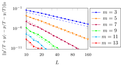
Figure 8.1: Maximum among the errors computed at $10001$ equidistant points in $[0,T]$ for different values of $m$ and $L$, compared to straight dashed lines having slope $m$.

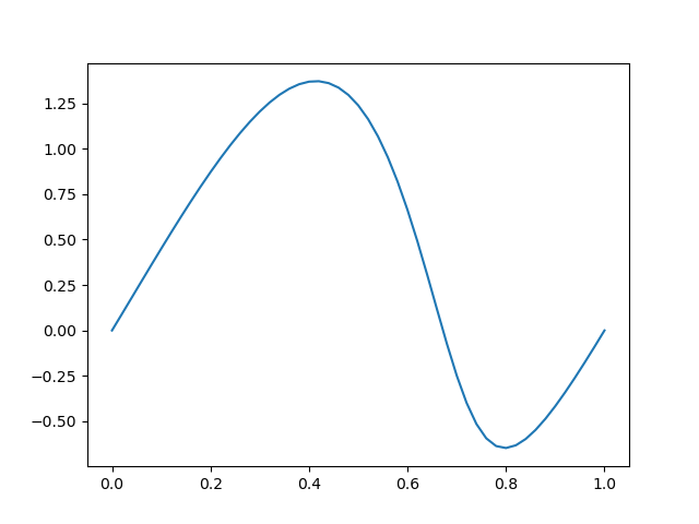
Figure 8.2: Periodic solution computed with $L=10$ and $m=5$, rescaled so as to have period 1.

9 Conclusions

In numerical bifurcation analysis of FDEs there is often a strong interest in analyzing the long-term dynamics. Such analysis includes the detection and computation of equilibria and periodic orbits regardless of their dynamical stability in a continuation framework with respect to model parameters.

The present paper provided a complete and rigorous error analysis of the piecewise orthogonal collocation for computing periodic solutions of FDEs which may include state-dependent delays. Indeed, although the method has widely been used for two decades (Engelborghs et al., 2002; Szalai, 2006) and incorporated into software such as DDE-Biftool and knut, the convergence of the corresponding finite-element method had only been supported by (many) numerical experiments but never proved theoretically for a general FDE.

A convergence analysis was recently performed for FDEs with constant delays (Andò and Breda, 2020), based on the general approach for BVPs established in (Maset, 2016). The latter assumes regularity properties on the part of the right-hand sides that cannot be satisfied when state-dependent delays are present. However, using the concepts of weaker forms of differentiability developed for state-dependent delays (Cassidy et al., 2019; Hartung et al., 2006), allowed us to arrive at convergence estimates as sharp as those previously obtained for constant delays by only assuming to satisfy the regularity properties in the milder form. In particular, our main result is the error estimate $O(L^{-\min\{\ell_{\max},m\}})$ for right-hand sides which are mildly differentiable to order $\ell_{\max}$, where $m$ is the fixed degree of the approximating piecewise polynomials and $L$ is the increasing size of the mesh. Moreover, we analyzed the convergence error of the corresponding Newton iterations with suitable regularization of the approximate solutions (in principle not well-defined at mesh points) that are found at each iteration.

The analysis carried out does not immediately extend to the spectral approach, characterized by bounded $L$ and increasing $m$, since it does assume in various points that the relevant interpolation operator is bounded. However, several of the apparent impediments to such an extension observed in (Andò and Breda, 2020) no longer hold once the BVP is formulated in periodic spaces of functions, as we have done in this paper. Therefore, the authors plan to reinvestigate the potential for spectral convergence for periodic BVPs of FDEs. Moreover, there is potential for extending the analysis to more general classes of delay equations, such as neutral FDEs, whose further restrictions on the regularity on the right-hand sides represent a substantial obstacle.

Appendix A Basic properties of mildly differentiable functions

A.1 Multi-dimensional extendability

The extendability condition 2 in Definition 2.1 is only formulated for the application of $\ell$ times the same deviation $\delta^{u}$. The polarization identity (Proposition A.2) ensures that condition 2 also applies to $\ell$ different deviations. In this subsection we use the notation $C^{\ell}$ for spaces of continuous $\ell=0$) or $\ell$ times continuously differentiable functions that are either periodic or defined on a closed bounded interval.

Lemma A.1 (Multidirectional extendability).

If $G$ is ${\ell_{\max}}$ times mildly differentiable according to Definition 2.1, then the map

$$C^{\ell}\times(C^{\ell})^{\ell}\ni(u,\delta^{u,1},\ldots,\delta^{u,\ell})\mapsto D^{\ell}G(u)\delta^{u,1}\ldots\delta^{u,\ell}\in\mathbb{R}^{n_{G}}$$

can be extended to a continuous map in $C^{\ell}\times(C^{\ell-1})^{\ell}$ for all $\ell\in\{1,\ldots,{\ell_{\max}}\}$.

Proposition A.2 (Polarization identity).

Let $\ell\geq 1$ be arbitrary. There exist $2^{\ell}$ coefficients $a_{i}\in\mathbb{R}$ and $\ell\,2^{\ell-1}$ coefficients $b_{i,j}\in\{-1,1\}$ ($i\in\{1,\ldots,2^{\ell-1}\}$, $j\in\{1,\ldots,\ell\}$) such that for all $c_{1},\ldots,c_{\ell}\in\mathbb{R}$ the following identity holds:

$$\prod_{j=1}^{\ell}c_{i}=\sum_{i=1}^{2^{\ell-1}}a_{i}\left[\sum_{j=1}^{\ell}b_{i,j}c_{j}\right]^{\ell}.$$

Consequently, for any bounded $\ell$-linear map $M$ from $X\times\ldots\times X$ to $Y$ and arbitrary linear spaces $X$ and $Y$

$$Mx_{1}\ldots x_{\ell}=\sum_{i=1}^{2^{\ell-1}}a_{i}M\left[\sum_{j=1}^{\ell}b_{i,j}x_{j}\right]^{\ell}\mbox{\quad for all $x_{1},\ldots,x_{\ell}\in X$.}$$

In short, arbitrary combinations of arguments of the multilinear map can be expressed as linear combination of the single-argument map $y\mapsto My^{\ell}$. For example, for $\ell=2$, the coefficients are $a_{1}=1/4$, $a_{2}=-1/4$, $b_{1,1}=b_{2,1}=b_{1,2}=1$, $b_{2,2}=-1$: $Myz=\frac{1}{4}M[y+z]^{2}-\frac{1}{4}M[y-z]^{2}$.

Proof of Lemma A.1

The proof is a continuity argument after recombining the multilinear expression $D^{\ell}G(u)\delta^{u,1}\ldots\delta^{u,\ell}$ as a linear combination of single-argument powers using the polarization identity Proposition A.2. Let $x\in C^{\ell}$, $y_{1},\ldots,y_{\ell}\in C^{\ell-1}$ be arbitrary, and let $y_{1,n},\ldots,y_{\ell,n}\in C^{\ell}$ be sequences such that $y_{i,n}\to y_{i}$ for $n\to\infty$ in the $C^{\ell-1}$-norm and $i\in\{1,\ldots,\ell\}$. Then

$$D^{\ell}G(x)y_{1,n}\ldots y_{\ell,n}=\sum_{i=1}^{2^{\ell-1}}a_{i}D^{\ell}G(x)\left[\sum_{j=1}^{\ell}b_{i,j}y_{j,n}\right]^{\ell}\to_{n\to\infty}\sum_{i=1}^{2^{\ell-1}}a_{i}D^{\ell}G(x)\left[\sum_{j=1}^{\ell}b_{i,j}y_{j}\right]^{\ell}.$$ (A.1)

The right-hand side is continuous in $(x,y_{1},\ldots,y_{\ell})\in C^{\ell}\times(C^{\ell-1})^{\ell}$ by Condition 2 of Definition 2.1. Thus, the left-hand side converges to a value. We call this value $D^{\ell}G(x)y_{1}\ldots y_{\ell}$ for $(x,y_{1},\ldots,y_{\ell})\in C^{\ell}\times(C^{\ell-1})^{\ell}$, such that the function

$$C^{\ell}\times(C^{\ell-1})^{\ell}\ni(x,y_{1},\ldots,y_{\ell})\mapsto D^{\ell}G(x)y_{1}\ldots y_{\ell}\in\mathbb{R}^{n_{G}}$$

is continuous. (end of proof for Lemma A.1)

A.2 Proof of Lemma 4.1

We first give the proof for ${\ell_{\max}}=1$ to illustrate the basic principle. The proof for ${\ell_{\max}}>1$ uses the same argument repeatedly. Recall that we have defined ${G_{\mathrm{ts}}}(x)(t)=G(x_{t})$ for an arbitrary $G:C^{0}_{\pi}\to\mathbb{R}^{n_{G}}$. We permit arbitrary dimensions for the arguments, so $x(t)\in\mathbb{R}^{n_{x}}$, $G(x_{t})\in\mathbb{R}^{n_{G}}$, where $n_{x}$ and $n_{G}$ do not have to be equal. We do not indicate the dimension of the function values in the space names, writing just $C^{k,j}_{\pi}$ to indicate regularity and periodicity.

Case ${\ell_{\max}}=1$

The fact that ${G_{\mathrm{ts}}}|_{C^{1}_{\pi}}:C^{1}_{\pi}\to C^{0}_{\pi}$ is continuously differentiable follows from the assumption that $G|_{C^{1}_{\pi}}:C^{1}_{\pi}\to\mathbb{R}^{n_{G}}$ is continuously differentiable such that we have the obvious candidate for the derivative $[D{G_{\mathrm{ts}}}(x)y](t)=DG(x_{t})y_{t}$, which is continuous because both maps $(C^{1}_{\pi})^{2}\ni(x,y)\mapsto DG(x)y\in\mathbb{R}^{n_{G}}$ and $\mathbb{R}\times(C^{1}_{\pi})^{2}\ni(t,x,y)\mapsto(x_{t},y_{t})\in(C^{1}_{\pi})^{2}$ are continuous.

The other part of the statement in Lemma 4.1 is that $C^{1}_{\pi}\ni x\mapsto{G_{\mathrm{ts}}}(x)\in C^{1}_{\pi}$ is continuous. Let us first check if ${G_{\mathrm{ts}}}(x)$ is in $C^{1}_{\pi}$: for small $h$ and arbitrary $t$, we express the finite-difference quotient for ${G_{\mathrm{ts}}}(x)(t)=G(x_{t})$

$$\frac{1}{h}[G(x_{t+h})-G(x_{t})]=\int_{0}^{1}DG(sx_{t+h}+(1-s)x_{t})\frac{x_{t+h}-x_{t}}{h}\mathop{}\!\mathrm{d}s.$$ (A.2)

On the left side the arguments of $G$ and $DG$, $x_{t+h}$, $x_{t}$ are both in $C^{1}_{\pi}$ by assumption. Thus, the functional $G$ is classically differentiable in $x_{t}$ and we can apply the mean value theorem to obtain the right-hand side in (A.2). As $x\in C^{1}_{\pi}$, the linear argument of $DG$, $(x_{t+h}-x_{t})/h$, converges to $x_{t}^{\prime}$ for $h\to 0$ in $C^{0}$-norm, while the nonlinear argument $sx_{t+h}+(1-s)x_{t}$ is in $C^{1}_{\pi}$ for all $s$, $t$ and $h$ and converges to $x_{t}$ for $h\to 0$ in the $C^{1}$-norm. By the continuous extendability condition of mild differentiability for $G$ the derivative $C^{1}\times C^{0}\ni(u,v)\mapsto DG(u)v$ is continuous such that the limit of the right-hand side of (A.2) for $h\to 0$ exists and equals $DG(x_{t})x_{t}^{\prime}$. Moreover, this term is continuous in $t$ by the continuous extendability condition 2 in Definition 2.1, and because $t\mapsto(x_{t},x_{t}^{\prime})\in C^{1}_{\pi}\times C^{0}_{\pi}$ is continuous for $x\in C^{1}_{\pi}$. Hence, the left-hand side in (A.2) has a limit for $h\to 0$ and is continuous in $t$.

We observe that we needed the extendability of $(x,y)\mapsto DG(x)y$ to $(x,y)\in C^{1}_{\pi}\times C^{0}_{\pi}$ to prove the “chain rule” that

$$({G_{\mathrm{ts}}}(x))^{\prime}(t)=(G(x_{t}))^{\prime}=DG(x_{t})x^{\prime}_{t}=[D{G_{\mathrm{ts}}}(x)(x^{\prime})](t).$$

Case ${\ell_{\max}}>1$

We repeat the above argument to show inductively over $k$ that

$$C^{k+\ell}_{\pi}\times(C^{k+\ell-1}_{\pi})^{\ell}\ni(x,y^{1},\ldots,y^{\ell})\mapsto D^{\ell}{G_{\mathrm{ts}}}(x)y^{1}\ldots y^{\ell}=\left[t\mapsto D^{\ell}G(x_{t})y^{1}_{t}\ldots y^{\ell}_{t}\right]\in C^{k}_{\pi}$$

is continuous, if $G$ is $k+\ell$ times mildly differentiable. The statement of Lemma 4.1 then follows from setting $k={\ell_{\max}}-\ell$.

For $k=0$ the fact that $D^{\ell}{G_{\mathrm{ts}}}|_{C^{\ell}_{\pi}}$ is well defined at each time $t$ follows from the assumption that $G$ is $\ell$ times mildly differentiable by definition. The continuity with respect to the $C^{0}_{\pi}$-norm in $t$ follows from the fact that the time shift

$$\mathbb{R}\times C^{j}_{\pi}\ni(t,u)\mapsto u_{t}\in C^{j}_{\pi}$$

is continuous for arbitrary $j\geq 0$.

For the inductive step, we first assume that for all integers $\ell\geq 0$ the function $t\mapsto D^{\ell}G(x_{t})y^{1}_{t}\ldots y^{\ell}_{t}$ is in $C^{k}_{\pi}$ for all $x\in C^{k+\ell}_{\pi}$ and all $y^{1},\ldots,y^{\ell}\in C^{k+\ell-1}_{\pi}$ if $G$ is $k+\ell$ times mildly differentiable. We have to show that $D^{\ell}G(x_{t})y^{1}_{t}\ldots y^{\ell}_{t}$ is in $C^{k+1}_{\pi}$ for $x\in C^{k+\ell+1}_{\pi}$, $y^{1},\ldots,y^{\ell}\in C^{k+\ell}_{\pi}$ if $G$ is $k+\ell+1$ times mildly differentiable. The time difference quotient for $D^{\ell}G(x_{t})y^{1}_{t}\ldots y^{\ell}_{t}$ at time $t$ equals

$$\frac{1}{h}\left[D^{\ell}G(x_{t+h})\prod_{i=1}^{\ell}y^{i}_{t+h}-D^{\ell}G(x_{t})\prod_{i=1}^{\ell}y^{i}_{t}\right]= \frac{1}{h}\left[D^{\ell}G(x_{t+h})\prod_{i=1}^{\ell}y^{i}_{t}-D^{\ell}G(x_{t})\prod_{i=1}^{\ell}y^{i}_{t}\right]+$$ (A.3)

$$\sum_{j=1}^{\ell}D^{\ell}G(x_{t})\prod_{i\neq j}^{\ell}y^{i}_{t}\frac{y^{j}_{t+h}-y^{j}_{t}}{h}$$ (A.4)

The function $u\mapsto D^{\ell}G(u)\prod_{i=1}^{\ell}y^{i}_{t}$ is continuously differentiable with respect to $u$ in $u=sx_{t+h}+(1-s)x_{t}$ for $s\in[0,1]$ since $x\in C^{k+\ell+1}_{\pi}$, $y^{1},\ldots,y^{k}\in C^{k+\ell}_{\pi}$ since $k\geq 1$ by the assumption that $G$ is $k+\ell+1$ times mildly differentiable and $u\in C^{k+\ell+1}_{\pi}$ and $y^{1},\ldots,y^{\ell}\in C^{k+\ell}_{\pi}$ with $k+\ell\geq\ell+1$. Thus, we may apply the mean-value theorem for the first term in the right-hand side of (A.3):

$$\frac{1}{h}\left[D^{\ell}G(x_{t+h})\prod_{i=1}^{\ell}y^{i}_{t}-D^{\ell}G(x_{t})\prod_{i=1}^{\ell}y^{i}_{t}\right]=\\ \int_{0}^{1}D^{\ell+1}G(sx_{t+h}+(1-s)x_{t})\frac{x_{t+h}-x_{t}}{h}\prod_{i=1}^{\ell}y^{i}_{t}\mathop{}\!\mathrm{d}s$$

By Lemma A.1 the derivative $D^{\ell+1}G(u)v_{0}\ldots v_{j}$ is continuous for arguments $u\in C^{\ell+1}_{\pi}$, $v_{0},\ldots,v_{\ell}\in C^{\ell}_{\pi}$. The argument $u=sx_{t+h}+(1-s)x_{t}$ is in $C^{k+\ell+1}_{\pi}$, $v_{0}=[x_{t+h}-x_{t}]/h$ is in $C^{k+\ell+1}_{\pi}$ and $y^{i}_{t}$ and the limit $x_{t}^{\prime}$ of $[x_{t+h}-x_{t}]/h$ are in $C^{k+\ell}_{\pi}$ such that we can take the limit for $h\to 0$ to obtain

$$\lim_{h\to 0}\frac{1}{h}\left[D^{\ell}G(x_{t+h})\prod_{i=1}^{\ell}y^{i}_{t}-D^{\ell}G(x_{t})\prod_{i=1}^{\ell}y^{i}_{t}\right]=D^{\ell+1}G(x_{t})x_{t}^{\prime}\prod_{i=1}^{\ell}y^{i}_{t}.$$

The right-hand side is a $C^{k}_{\pi}$ function by the assumption of the inductive step.

In the terms in (A.4) the difference quotient $[y^{j}_{t+h}-y^{j}_{t}]/h$ has the limit $(y^{j}_{t})^{\prime}$ in $C^{k+\ell-1}_{\pi}$ and the derivative $D^{\ell}G(x_{t})$ can be extended continuously to multilinear arguments in $C^{k+\ell-1}_{\pi}$, since $G$ is $k+\ell\geq\ell$ times mildly differentiable. Thus, the limit for $h\to 0$ also exists for the terms in (A.4):

$$\lim_{h\to 0}D^{\ell}G(x_{t})\prod_{i\neq j}^{\ell}y^{i}_{t}\frac{y^{j}_{t+h}-y^{j}_{t}}{h}=D^{\ell}G(x_{t})\prod_{i\neq j}y^{i}_{t}(y^{j}_{t})^{\prime}.$$ (A.5)

The argument $x$ in this limit is in $C^{k+\ell+1}_{\pi}$, the arguments $y^{i}_{t}$ are in $C^{k+\ell}_{\pi}$ and $(y^{j})^{\prime}$ is in $C^{k+\ell-1}_{\pi}$. Thus, by the assumption in the inductive step the limits in (A.5) are also in $C^{k}_{\pi}$ for $j=1\ldots,\ell$. This implies that the sum of the limits of the right-hand side terms in (A.3), (A.4), and, thus, the limit of the time difference quotient in (A.3) are in $C^{k}_{\pi}$. Hence, $t\mapsto D^{\ell}G(x_{t})y^{1}_{t}\ldots y^{\ell}_{t}$ is in $C^{k+1}_{\pi}$.

Finally, let us check the continuity of the map

$$C^{k+\ell+1}_{\pi}\times(C^{k+\ell}_{\pi})^{\ell}\ni(x,y^{1},\ldots,y^{\ell})\mapsto D^{\ell}{G_{\mathrm{ts}}}(x)y^{1}\ldots y^{\ell}\in C^{k+1}_{\pi}.$$

By inductive assumption the map is continuous as a map into $C^{k}_{\pi}$. According to (A.3),(A.4) and (A.5), its highest derivative in $t$ equals

$$D^{\ell+1}G(x_{t})x_{t}^{\prime}\prod_{i=1}^{\ell}y^{i}_{t}+\sum_{j=1}^{\ell}D^{\ell}G(x_{t})\prod_{i\neq j}^{\ell}y^{i}_{t}(y^{j}_{t})^{\prime}.$$

All terms in this sum are continuously mapping $C^{k+\ell+1}_{\pi}\times(C^{k+\ell}_{\pi})^{\ell}\ni(x,y^{1},\ldots,y^{\ell})$ into $C^{k}_{\pi}$ by inductive assumption, such that $(x,y^{1},\ldots,y^{\ell})\mapsto D^{\ell}{G_{\mathrm{ts}}}(x)y^{1}\ldots y^{\ell}$ is continuous into $C^{k+1}_{\pi}$.

(end of proof for Lemma 4.1)

A.3 Proof of Corollary 4.2

Corollary 4.2 follows directly from the continuity of the map $C^{1}_{\pi}\times C^{0}_{\pi}\ni(u,\delta^{u})\mapsto D{G_{\mathrm{ts}}}(u)\delta^{u}\in C^{0}_{\pi}$, because continuously differentiable functions are dense in the space of Lipschitz continuous functions with respect to the $C^{0}$-norm. The limit (4.2) holds for $v,w\in C^{1}_{\pi}$ by definition of mild differentiability of $G$ and Lemma 4.1 (with ${\ell_{\max}}=\ell=1$). Thus, choosing sequences $C^{1}_{\pi}\ni v^{n}\to v\in C^{0,1}_{\pi}$ and $C^{1}_{\pi}\ni w^{n}\to w\in C^{0,1}_{\pi}$ that converge in the $C^{0}$-norm, and choosing $n$ sufficiently large (depending on $v$ and $w$), also ensures the same limit for $v$, $w\in C^{0,1}_{\pi}$.

(end of proof for Corollary 4.2)

Appendix B Results for DDEs implying Assumptions 5.1 and 5.4

The theoretical results by Sieber and Szalai (2011) and Sieber (2012) provide some criteria that imply Assumptions 5.1 and 5.4, required by our analysis. In particular, Sieber (2012) proves that the Hopf bifurcation theorem also holds for DDEs with state-dependent delay. This theorem ensures existence of small-amplitude periodic orbits near an equilibrium satisfying eigenvalue conditions Kuznetsov (2004). Our claim that example (1.3) has small-amplitude periodic orbits for parameters $p\approx\pi/2$ is based on the Hopf bifurcation theorem. Th central result in each of both papers, (Sieber and Szalai, 2011; Sieber, 2012), is a reduction of a DDE to a finite-dimensional system of equations. Sieber and Szalai (2011) reduces the eigenvalue problem of a monodromy operator of a linear time-periodic DDE to an eigenvalue problem for a finite-dimensional characteristic matrix. Sieber (2012) reduces a nonlinear periodic BVP for DDEs with state-dependent delay to a finite-dimensional system of algebraic equations. In both cases the result was stated for problems without parameters. However, the proof of the Hopf bifurcation theorem in (Sieber, 2012) shows that one can apply the results also to problems with parameters by applying a trivial extension, treating the parameters $\mu$ as time-dependent variables satisfying the equation $\mu^{\prime}(t)=0$. This extension permits us to formulate solvability assumptions on finite-dimensional equations that imply Assumptions 5.1 and 5.4.

B.1 Results for nonlinear DDEs with state-dependent delays implying existence (Assumption 5.1)

Sieber (2012) considered a $\ell\geq 1$ times mildly differentiable nonlinear functional $G:C([-\tau_{\max},0];\mathbb{R}^{n_{y}})\to\mathbb{R}^{n_{y}}$ and a sufficiently small ball $B^{0,1}_{r}(y^{*})\subset C^{0,1}_{\pi}$ around an arbitrary function $y^{\mathrm{c}}\in C^{1,1}_{\pi}$. Denoting the projection onto the first $m$ Fourier coefficients of $y^{\mathrm{c}}$ by $y^{\mathrm{c},m}\in\mathbb{R}^{n_{y}(2m+1)}$, they constructed maps $Y^{m}:B_{r}(y^{\mathrm{c}.m})\to C^{0}_{\pi}$ and $G^{m}:B_{r}(y^{\mathrm{c},m})\to\mathbb{R}^{n_{y}(2m+1)}$ such that all $y\in B^{0,1}_{r}(y^{\mathrm{c}})$ satisfy the equivalence

$y^{\prime}(t)=G(y_{t})$ if and only if $y=Y^{m}(y^{m})$ and $G^{m}(y^{m})=0$,

where $y^{m}$ is the projection of $y$ onto its first $m$ Fourier coefficients. The maps $G^{m}$ and $Y^{m}$ are continuously differentiable $\ell$ times. So, the result reduces the nonlinear periodic boundary-value problem $y^{\prime}=G(y_{t})$ locally to an algebraic system of equations $y^{m}=G^{m}(y^{m})$ with a $\ell$ times continouusly differentiable right-hand side $G^{m}$.

While this statement is formulated for parmeter-independent problems, we may treat the system parameters $\mu$ as trivial (constant) period-$1$ functions by including them initially as dynamic variables with the trivial differential equation $\mu^{\prime}(t)=0$, extending the nonlinear FDE $y^{\prime}(t)=G(y_{t},\mu)$ in (3.2) to

$$v^{\prime}(t) =G(v_{t},\mu),\quad\mu^{\prime}(t)=0.$$ (B.1)

Applying the result in (Sieber, 2012) to this extended system (B.1) produces $\ell$ times continuously differentiable maps extended maps $Y^{m}_{\mathrm{e}}$ and $G^{m}_{\mathrm{e}}$ near $(y^{\mathrm{c},m},\mu^{\mathrm{c}})$, where $G^{m}_{\mathrm{e}}$ contains $n_{\mu}$ trivial (identical zero) components. Hence, we may state the following finite-dimensional condition implying Assumption 5.1.

Corollary B.1 (Equivalent condition for existence of solution).

Let $(y^{\mathrm{c}},\mu^{\mathrm{c}})\in C^{1,1}_{\pi}\times\mathbb{R}^{n_{\mu}}$ be arbitrary and the radius $r$ be sufficiently small such that the maps $G^{m}_{\mathrm{e}}$ and $Y^{m}_{\mathrm{e}}$ exist on $B^{0,1}((y^{\mathrm{c},m},\mu^{\mathrm{c}}))$. Then the fixed-point problem $x=\Phi(x)$ has a solution $x^{*}=(v^{*},\alpha^{*},\mu^{*})$ in $B^{0,1}_{r}((y^{\mathrm{c}},\mu^{\mathrm{c}}))$ with $\alpha^{*}=v^{*}(0)$ if and only if the $((n_{y}+n_{\mu})(2m+1)+n_{\mu})$-dimensional system of algebraic equations

$$0 =G^{m}_{\mathrm{e}}(y^{m},\mu^{m})$$

$$0 =R_{\mathrm{aff}}[Y^{m}_{\mathrm{e}}(y^{m},\mu^{m}),\mu^{m}]$$

has a solution $(v^{*,m},\mu^{*,m})$ and $(v^{*},\mu^{*})=Y^{m}_{\mathrm{e}}(v^{*,m},\mu^{*,m})$.

The extension by $\mu^{\prime}=0$ was also used in (Sieber, 2012) to prove the Hopf bifurcation theorem, which provides conditions for the existence of periodic orbits near an equilibrium with verifiable conditions.

B.2 Results for linear time-periodic DDEs implying linear invertibility (Assumption 5.4)

Let us now assume that we have a a given problem (3.2) with proposed solution $x^{*}$. For the right-hand side $G$ of DDE (3.2), the Fréchet derivative $D_{v}G(v^{*}_{t},\mu^{*})$ w.r.t. $v$ is a continuous linear functional from $C^{0}_{\pi}$ to $\mathbb{R}^{n_{y}}$ that is also continuous and periodic in $t$. If the “maximal delay in the DDE is finite”, that is, if $G$ is well defined and mildly differentiable as a functional from $C^{0}([-\tau_{\max},0];\mathbb{R}^{n_{y}})\times\mathbb{R}^{\mu}$ to $\mathbb{R}^{n_{y}}$ for some finite integer $\tau_{\max}$, then there exists a function $\eta^{*}:\mathbb{R}\times[0,\tau_{\max}]\ni(t,\theta)\mapsto\eta(t,\theta)\in\mathbb{R}^{n_{y}\times n_{y}}$ that is continuous in its first argument $t$, and right-continuous and of bounded variation in its second argument $\theta$ such that

$$D_{v}G(v^{*},\mu^{*})\delta^{v}=\int_{0}^{\tau_{\max}}\mathop{}\!\mathrm{d}\eta^{*}(t,\theta)\delta^{v}(t-\theta).$$

Properties of the linear DDE $(\delta^{v})^{\prime}=D_{v}G(v^{*},\mu^{*})\delta^{v}$ are then determined by the spectral properties of the monodromy operator $M:C^{0}([-\tau_{\max},0];\mathbb{R}^{n_{y}})\to C^{0}([-\tau_{\max},0];\mathbb{R}^{n_{y}})$, given by $[M\delta^{v}](s)=u(1+s)$ for $s\in[-\tau_{\max},0]$, $\delta^{v}\in C^{0}([-\tau_{\max},0];\mathbb{R}^{n_{y}})$ and $u\in C^{0}([-\tau_{\max},1];\mathbb{R}^{n_{y}})$ where

$$u^{\prime}(t) =\int_{0}^{\tau_{\max}}\mathop{}\!\mathrm{d}\eta^{*}(t,\theta)u(t-\theta) t\in(0,1)$$ for , (B.2)

$$u(t) =\delta^{v}(t) t\in[-\tau_{\max},0]$$ for . (B.3)

Sieber and Szalai (2011) reduced eigenvalue problems for the monodromy operator $M$ to an equivalent eigenvalue problem $\Delta(\lambda)u_{\Delta}=0$. The characteristic matrix $\Delta(\lambda)\in\mathbb{C}^{n_{\Delta}\times n_{\Delta}}$ is analytic in $\lambda$ for all $\lambda\in\mathbb{C}$ with $|\lambda|<R_{\max}$, where $R_{\max}$ is an arbitrary large bound. The dimension $n_{\Delta}$ of $\Delta$ depends on the total variation of $\eta^{*}$ and on $R_{\max}$. The $\lambda$ with $|\lambda|<R_{\max}$ for which $\Delta(\lambda)$ is singular are the inverses of the Floquet multipliers of (B.2) with modulus greater than $1/R_{\max}$. Furthermore, the construction by Sieber and Szalai (2011) creates a linear map

$$E(\lambda):\mathbb{C}^{n_{\Delta}}\ni u_{\Delta}\mapsto u\in C^{1}([-\tau_{\max},1];\mathbb{R}^{n_{y}})\mbox{\quad s.t. for\ }u=E(\lambda)u_{\Delta}$$

$$\Delta(\lambda)u_{\Delta}=0\mbox{\ if and only if $u$ satisfies \eqref{lin:dde} and\ }u(t+1)\lambda=u(t)\mbox{\ for all $t\in[-\tau_{\max},0]$},$$

such that $u|_{[-\tau_{\max},0]}$ is eigenvector of $M$. The map $E(\lambda)$ is also analytic in $\lambda$ for $|\lambda|<R_{\max}$. Moreover, Sieber and Szalai (2011) showed that the map $E$ establishes an equivalence between eigenvalue problems for $M$ and $\Delta(\lambda)$ in the sense of Kaashoek and Verduyn Lunel (1992): $\lambda$ is an eigenvalue of the nonlinear eigenvalue problem $\Delta(\lambda)u_{\Delta}=0$ of geometric multiplicity $\operatorname{GM}(\lambda)$ and algebraic multiplicity $\operatorname{AM}(\lambda)$ if and only if $\lambda$ is an eigenvalue with same geometric and algebraic multiplicity for the eigenvalue problem of the monodromy operator $M$. The map $u_{\Delta}\mapsto[E(\lambda)u_{\Delta}]|_{[-\tau_{\max},0]}$ maps generalized eigenspaces of $\Delta(\lambda)$ onto the generalized eigenspaces of $M$ for $\lambda$.

Hence, we may use the characteristic matrix $\Delta(\lambda)$ also to construct a criterion for Assumption 5.4 treat the system parameters $\mu$ as trivial (constant) period-$1$ functions by including them initially as dynamic variables with the trivial differential equation $\mu^{\prime}(t)=0$. So, we extend the nonlinear FDE $y^{\prime}(t)=G(y_{t},\mu)$ in (3.2) to (B.1) in the solution $(v^{*},\mu^{*})$ of the fixed-point problem. The linearization of (B.1) in $(v^{*},\mu^{*})$ has then the trivially extended monodromy operator

$$M_{\mathrm{e}}\begin{bmatrix}\delta^{v}\\ \delta^{\mu}\end{bmatrix} =\begin{bmatrix}M_{\mathrm{e}}^{v}[\delta^{v},\delta^{\mu}]\\ M_{\mathrm{e}}^{\mu}[\delta^{v},\delta^{\mu}]\end{bmatrix}\mbox{,\quad where} \begin{matrix}M_{\mathrm{e}}^{v}[\delta^{v},\delta^{\mu}](s)=u^{v}(1+s)\\ M_{\mathrm{e}}^{\mu}[\delta^{v},\delta^{\mu}](s)=u^{\mu}(1+s)\end{matrix}$$

for $s\in[-\tau_{\max},0]$ and

$$\begin{bmatrix}(u^{v})^{\prime}(t)\\ (u^{\mu})^{\prime}(t)\end{bmatrix} =\begin{bmatrix}\int_{0}^{\tau_{\max}}\mathop{}\!\mathrm{d}\,[\eta_{v}^{*}(t,\theta)u^{v}(t-\theta)+\eta_{\mu}^{*}(t,\theta)u^{\mu}(t-\theta)]\\ 0\end{bmatrix} t\in(0,1)$$ for ,

$$\begin{bmatrix}(u^{v})(t)\\ (u^{\mu})(t)\end{bmatrix} =\begin{bmatrix}(\delta^{v})(t)\\ (\delta^{\mu})(t)\end{bmatrix} t\in[-\tau_{\max},0]$$ for .

The operator $M_{\mathrm{e}}^{\mu}$ satisfies $M_{\mathrm{e}}^{\mu}[0,\delta^{\mu}]=\delta^{\mu}$, such that $M_{\mathrm{e}}$ will have eigenvalue $1$ with at least geometric multiplicity $n_{\mu}$, and eigenspace $\{(\delta^{v},\delta^{\mu}):\delta^{\mu}=\operatorname{const},M_{\mathrm{e}}^{v}[\delta^{v},\delta^{\mu}]=\delta^{v}\}$. By the the equivalence statement of Sieber and Szalai (2011) the characteristic matrix $\Delta_{\mathrm{e}}(\lambda)$ for the extended monodromy operator $M_{\mathrm{e}}$ (of dimension $n_{\Delta,\mathrm{e}})$ will have a nullspace of dimension at least $n_{\mu}$ at $\lambda=1$: $\dim\ker\Delta_{\mathrm{e}}(1)\geq n_{\mu}$.

Assumption 5.4 is equivalent to the condition that $\dim\ker\Delta_{\mathrm{e}}(1)=n_{\mu}$, and that the $n_{\mu}$ affine conditions $R_{\mathrm{aff}}$ in the fixed-point problem (3.5) have full rank on $\ker\Delta_{\mathrm{e}}(1)$.

Corollary B.2 (Equivalent condition for well-posedness of linear problem).

The linear operator $I-D\Phi(x^{*})$ for $x^{*}=(v^{*},\alpha^{*},\mu^{*})$ is injective on $C^{1}_{\mathrm{e}}$ if and only if the matrix

$$\Delta_{\Phi}(v^{*},\mu^{*})=\begin{bmatrix}\Delta_{\mathrm{e}}(v^{*},\mu^{*};1)\\ DR_{\mathrm{aff}}\end{bmatrix}\in\mathbb{R}^{(n_{\Delta,\mathrm{e}}+n_{\mu})\times n_{\Delta,\mathrm{e}}}$$

has full rank $n_{\Delta,\mathrm{e}}$.

We included the base point $(v^{*},\mu^{*})$ of the linearization as explicit argument of $\Delta_{\Phi}$ and $\Delta_{\mathrm{e}}$, in addition to the eigenvalue $\lambda$ (equal to $1$ here), to indicate that this is a condition on the solution $x^{*}=(v^{*},\alpha^{*},\mu^{*})$.

Constructions of characteristic matrices for periodic linear FDEs have been generalized to FDEs of neutral type by Verduyn Lunel (2023). The construction of $\Delta(\lambda)$ in (Sieber and Szalai, 2011) is primarily useful for proving the existence of a characteristic matrix for periodic problems. In practice numerical methods for determining eigenvalues of monodromy operators, such as the pseudospectral method (Breda et al., 2006, 2012), work directly on large matrices generated by the discretization projection $\mathcal{P}_{L}$, without prior reduction. Borgioli et al. (2020) proves convergence of methods as implemented in DDE-Biftool and knut.

Appendix C Approximation properties of regularization

This section confirms some basic properties of the regularization as proposed in (7.2) in Section 7.1. Let us first check in an example how the limit $\lim_{\rho\to 0}DG(S_{\rho}y_{t},\mu)$ could look.

Example

For the simple example $G$ in (1.3), $G(y,T,p)=-Ty(-p/T-y(0)/T)$, the different $\sigma$ correspond to using convex combinations of one-sided limits at discontinuities of $y^{\prime}$. The expression $DG(y,T,p)[\delta^{y},\delta^{T},\delta^{p}]$ contains the term $y^{\prime}(-p/T-y(0)/T)$, as (1.7) shows. Thus, if $y$ is a piecewise continuous polynomial,

$$\lim_{s\to 0}DG(S_{\rho}y_{t_{i,j}},T,p)[\delta^{y}_{t_{i,j}},\delta^{T},\delta^{p}]= \ (1-\sigma)\lim_{t\uparrow t_{i,j}}DG(y_{t},T,p)[\delta^{y}_{t},\delta^{T},\delta^{p}]$$

$$\phantom{\ (1}+\sigma\phantom{)}\lim_{t\downarrow t_{i,j}}DG(y_{t},T,p)[\delta^{y}_{t},\delta^{T},\delta^{p}]$$

$$\mbox{using\quad}(1-\sigma)\lim_{t\uparrow t_{i,j}}y^{\prime} (t-p/T-y(t)/T)+\sigma\lim_{t\downarrow t_{i,j}}y^{\prime}(t-p/T-y(t)/T)\mbox{}$$

if $t_{i,j}-p/T-y(t_{i,j})/T-t_{k}\in\mathbb{Z}$ for some $i,k\in\{1,\ldots,L\}$, $j\in\{1,\ldots,m\}$.

Proposition C.1 (Distance of smoothed $C^{0,1}$ function from $C^{1,1}$ function).

The operator $S_{\rho}$ satisfies

$$\|S_{\rho}u-v\|_{0} \leq\|u-v\|_{\infty}+\rho\|v\|_{0,1}\mbox{\quad for all $u\in L^{\infty}_{\pi}$, $v\in C^{0,1}_{\pi}$, $\rho>0$, $\sigma\in[0,1]$,}$$

$$\|S_{\rho}u-v\|_{1} \leq\|u-v\|_{0,1}+\rho\|v\|_{1,1}\mbox{\quad for all $u\in C^{0,1}_{\pi}$, $v\in C^{1,1}_{\pi}$, $\rho>0$, $\sigma\in[0,1]$.}$$

Proof.

Let $u\in L^{\infty}_{\pi}$ and $v\in C^{0,1}_{\pi}$ be arbitrary. We split

$$\frac{1}{\rho}\int_{t+\rho\sigma-\rho}^{t+\rho\sigma}u(s)\mathop{}\!\mathrm{d}s-v(t) =\frac{1}{\rho}\int_{t+\rho\sigma-\rho}^{t+\rho\sigma}u(s)-v(s)\mathop{}\!\mathrm{d}s+\frac{1}{\rho}\int_{t+\rho\sigma-\rho}^{t+\rho\sigma}v(s)-v(t)\mathop{}\!\mathrm{d}s,$$

hence,

$$\|S_{\rho}u-v\|_{0} \leq\|u-v\|_{\infty}+\frac{\operatorname{Lip}v}{\rho}\int_{t+\rho\sigma-\rho}^{t+\rho\sigma}|s-t|\mathop{}\!\mathrm{d}s\leq\|u-v\|_{\infty}+\rho\operatorname{Lip}v.$$ (C.1)

Let now also be $u\in C^{0,1}_{\pi}$ and $v\in C^{1,1}_{\pi}$. Then we have for the derivative

$$|[S_{\rho}u]^{\prime}(t)-v^{\prime}(t)|= \ \left|\frac{1}{\rho}\left[u(t+\rho\sigma)-u(t+\rho\sigma-\rho)-(v(t+\rho\sigma)-v(t+\rho\sigma-\rho))\right]\right.$$

$$\ \left.+\frac{1}{\rho}[v(t+\rho\sigma)-v(t+\rho\sigma-\rho)]-v^{\prime}(t)\right|$$

$$\leq\operatorname{Lip}[u-v]+\rho\operatorname{Lip}v^{\prime}.$$ (C.2)

Thus, combining (C.1) and (C.2), we obtain the estimates of Proposition C.1. ∎

Appendix D Proof of Lemma 7.2 about convergence of Newton iteration

Let us denote $D\Phi_{L}(x^{*})-I$ and its inverse (known to exist for $L>L_{\mathrm{low}}(\epsilon)$ in (6.16)) by

$$DF_{L}^{*} :=D\Phi_{L}(x^{*})-I, [DF_{L}^{*}]^{-1} :=[D\Phi_{L}(x^{*})-I]^{-1}.$$

An upper bound for the norm $\|[DF_{L}^{*}]^{-1}\|_{C^{0,1}_{\mathrm{e}}\leftarrow C^{0,1}_{\mathrm{e}}}$ was introduced as $C_{\mathrm{stab},L}$ in Corollary 6.3, equation (6.10). By construction of $R_{\mathrm{d}}$ and $R_{\mathrm{s}}$ and the formulation of the modified Newton iteration (7.1) we have

$$\delta^{k+1}_{L}=\ \delta^{k}_{L}-\left[DF_{L}^{*}+R_{\mathrm{d}}(S_{\rho}x^{k}_{L}-x^{*})\right]^{-1}\left[(DF_{L}^{*})\,\delta^{k}_{L}+R_{\mathrm{s}}(\delta^{\infty}_{L},\delta^{k}_{L})\right]$$

$$=\ \left[DF_{L}^{*}+R_{\mathrm{d}}(S_{\rho}x^{k}_{L}-x^{*})\right]^{-1}\left[R_{\mathrm{d}}(S_{\rho}x^{k}_{L}-x^{*})\delta^{k}_{L}-R_{\mathrm{s}}(\delta^{\infty}_{L},\delta^{k}_{L})\right].$$

All quantities have $C^{0,1}$-norms. We know by (7.9) that for all $y\in C^{0,1}_{\mathrm{e}}$

$$\|R_{\mathrm{d}}(S_{\rho}x^{k}_{L}-x^{*})y\|_{0,1} \leq\omega_{\mathrm{d}}(\|S_{\rho}x^{k}_{L}-x^{*}\|_{1})\|y\|_{0,1}.$$

For the argument $S_{\rho}x^{k}_{L}-x^{*}$ we have by approximation property (2.6)

$$\|S_{\rho}x^{k}_{L}-x^{*}\|_{1} \leq\|\|x^{k}_{L}-x^{*}\|_{0,1}+\rho\|x^{*}\|_{1,1}$$

$$\leq\|x^{k}_{L}-x^{\infty}_{L}\|_{0,1}+\|x^{\infty}_{L}-x^{*}\|_{0,1}+\rho\|x^{*}\|_{1,1}$$

$$\leq\|\delta^{k}_{L}\|_{0,1}+\|\delta^{\infty}_{L}\|_{0,1}+\rho\|x^{*}\|_{1,1}.$$

Thus, for sufficiently small $\rho_{\max}$, large $L_{\mathrm{nwt}}$ and small initial radius $r_{\mathrm{nwt}}$ for $\delta^{k}_{L}$, we can make $\|R_{\mathrm{d}}(S_{\rho}x^{k}_{L}-x^{*})\|_{C^{0,1}_{\mathrm{e}}\leftarrow C^{0,1}_{\mathrm{e}}}$ arbitrarily small. Hence, for arbitrary small $\epsilon$ and sufficiently small $\rho_{\max}$, large $L_{\mathrm{nwt}}$ and small radius $r_{\mathrm{nwt}}$ we have by the Banach Perturbation Lemma

$$\|[DF_{L}^{*}+R_{\mathrm{d}}(S_{\rho}x^{k}_{L}-x^{*})]^{-1}\|_{C^{0,1}_{\mathrm{e}}\leftarrow C^{0,1}_{\mathrm{e}}} \leq C_{\mathrm{stab},L}(1+\epsilon/2)\leq C_{\mathrm{stab},\infty}(1+\epsilon)$$

since $C_{\mathrm{stab},L}\to C_{\mathrm{stab},\infty}$ for $L\to\infty$. This bound and the bounds (7.8) and (7.9) for $R_{\mathrm{d}}$ and $R_{\mathrm{s}}$ and $S_{\rho}x^{k}_{L}-x^{*}$ imply

$$\cfrac{\|\delta^{k+1}\|_{0,1}}{\|\delta^{k}\|_{0,1}}\leq C_{\mathrm{stab},\infty}(1+\epsilon)\left[\omega_{\mathrm{d}}(\|\delta^{k}\|_{0,1}\!+\!\|\delta^{\infty}\|_{0,1}\!+\!\rho\|x^{*}\|_{1,1})+\omega_{\mathrm{d}}(\|\delta^{k}\|_{0,1}\!+\!2\|\delta^{\infty}\|_{0,1})\right]\!,$$

which is the estimate (7.10).

References

• Ahsan et al. (2022) Z. Ahsan, H. Dankowicz, M. Li, and J. Sieber. Methods of continuation and their implementation in the coco software platform with application to delay differential equations. Nonlinear Dynamics, 107(4):3181–3243, 2022.
• Andò (2020) A. Andò. Collocation methods for complex delay models of structured populations. PhD thesis, University of Udine, 2020. http://cdlab.uniud.it/theses/Ando2020.pdf.
• Andò and Breda (2020) A. Andò and D. Breda. Convergence analysis of collocation methods for computing periodic solutions of retarded functional differential equations. SIAM Journal on Numerical Analysis, 58(5):3010–3039, 2020.
• Arnold (2001) D. Arnold. A concise introduction to numerical analysis. http://www.ima.umn.edu/~arnold/597.00-01/nabook.pdf, 2001.
• Ascher et al. (1981) U. Ascher, J. Christiansen, and R. D. Russell. Collocation software for boundary-value odes. ACM Transactions on Mathematical Software (TOMS), 7(2):209–222, 1981.
• Barton et al. (2006) D. Barton, B. Krauskopf, and R. Wilson. Collocation schemes for periodic solutions of neutral delay differential equations. Journal of Difference Equations and Applications, 12(11):1087–1101, 2006.
• Borgioli et al. (2020) F. Borgioli, D. Hajdu, T. Insperger, G. Stepan, and W. Michiels. Pseudospectral method for assessing stability robustness for linear time-periodic delayed dynamical systems. International Journal for Numerical Methods in Engineering, 121(16):3505–3528, 2020.
• Breda et al. (2005) D. Breda, S. Maset, and R. Vermiglio. Pseudospectral differencing methods for characteristic roots of delay differential equations. SIAM Journal on Scientific Computing, 27(2):482–495, 2005.
• Breda et al. (2006) D. Breda, S. Maset, and R. Vermiglio. Numerical computation of characteristic multipliers for linear time periodic delay differential equations. In C. Manes and P. Pepe, editors, Time Delay Systems 2006, volume 6 of IFAC Proceedings Volumes. Elsevier, 2006.
• Breda et al. (2012) D. Breda, S. Maset, and R. Vermiglio. Approximation of eigenvalues of evolution operators for linear retarded functional differential equations. SIAM J. Numer. Anal., 50(3):1456–1483, 2012.
• Cassidy et al. (2019) T. Cassidy, M. Craig, and A. R. Humphries. Equivalences between age structured models and state dependent distributed delay differential equations. Mathematical Biosciences and Engineering, 16(5):5419–5450, 2019.
• Dankowicz and Schilder (2013) H. Dankowicz and F. Schilder. Recipes for Continuation. Computer Science and Engineering. SIAM, 2013.
• Desroches et al. (2012) M. Desroches, J. Guckenheimer, B. Krauskopf, C. Kuehn, H. M. Osinga, and M. Wechselberger. Mixed-mode oscillations with multiple time scales. SIAM Review, 54(2):211–288, 2012.
• Diekmann et al. (1995) O. Diekmann, S. van Gils, S. Verduyn Lunel, and H.-O. Walther. Delay equations, volume 110 of Applied Mathematical Sciences. Springer-Verlag, New York, 1995.
• Diekmann et al. (2010) O. Diekmann, M. Gyllenberg, J. A. Metz, S. Nakaoka, and A. M. de Roos. Daphnia revisited: local stability and bifurcation theory for physiologically structured population models explained by way of an example. Journal of mathematical biology, 61(2):277–318, 2010.
• Doedel (2007) E. J. Doedel. Lecture notes on numerical analysis of nonlinear equations. In B. Krauskopf, H. M. Osinga, and J. Galán-Vioque, editors, Numerical Continuation Methods for Dynamical Systems: Path following and boundary value problems, pages 1–49. Springer-Verlag, Dordrecht, 2007.
• Engelborghs and Doedel (2002) K. Engelborghs and E. J. Doedel. Stability of piecewise polynomial collocation for computing periodic solutions of delay differential equations. Numerische Mathematik, 91(4):627–648, 2002.
• Engelborghs et al. (2001) K. Engelborghs, T. Luzyanina, K. I. Hout, and D. Roose. Collocation methods for the computation of periodic solutions of delay differential equations. SIAM Journal on Scientific Computing, 22(5):1593–1609, 2001.
• Engelborghs et al. (2002) K. Engelborghs, T. Luzyanina, and D. Roose. Numerical bifurcation analysis of delay differential equations using DDE-BIFTOOL. ACM Transactions on Mathematical Software, 28(1):1–21, 2002.
• Gedeon et al. (2022) T. Gedeon, A. R. Humphries, M. C. Mackey, H.-O. Walther, and Z. Wang. Operon dynamics with state dependent transcription and/or translation delays. Journal of Mathematical Biology, 84(1):2, 2022.
• Govaerts and Kuznetsov (2007) W. Govaerts and Y. Kuznetsov. Interactive continuation tools. In B. Krauskopf, H. M. Osinga, and J. Galán-Vioque, editors, Numerical Continuation Methods for Dynamical Systems: Path following and boundary value problems, pages 51–75. Springer-Verlag, Dordrecht, 2007.
• Hale (1977) J. Hale. Theory of Functional Differential Equations. Applied mathematical sciences. Springer-Verlag, 1977. ISBN 9780387902036.
• Hale and Verduyn Lunel (1993) J. Hale and S. Verduyn Lunel. Introduction to functional-differential equations, volume 99 of Applied Mathematical Sciences. Springer-Verlag, New York, 1993.
• Hartung et al. (2006) F. Hartung, T. Krisztin, H.-O. Walther, and J. Wu. Functional differential equations with state-dependent delays: theory and applications. In P. Drábek, A. Cañada, and A. Fonda, editors, Handbook of Differential Equations: Ordinary Differential Equations, volume 3, chapter 5, pages 435–545. North-Holland, 2006.
• Insperger et al. (2008) T. Insperger, D. A. W. Barton, and G. Stépán. Criticality of Hopf bifurcation in state-dependent delay model of turning processes. International Journal of Non-Linear Mechanics, 43(2):140 – 149, 2008.
• Kaashoek and Verduyn Lunel (1992) M. A. Kaashoek and S. M. Verduyn Lunel. Characteristic matrices and spectral properties of evolutionary systems. Trans. Amer. Math. Soc., 334(2):479–517, 1992.
• Keller (1975) H. Keller. Approximation methods for nonlinear problems with application to two-point boundary value problems. Mathematics of Computation, 29(130):464–474, 1975.
• Kincaid and Cheney (2002) D. Kincaid and W. Cheney. Numerical Analysis - Mathematics of Scientific Computing. Number 2 in Pure and Applied Undergraduate Texts. American Mathematical Society, Providence, 2002.
• Kuznetsov (2004) Y. A. Kuznetsov. Elements of Applied Bifurcation Theory, volume 112 of Applied Mathematical Sciences. Springer-Verlag, New York, third edition, 2004. ISBN 0-387-21906-4.
• Maset (2015a) S. Maset. The collocation method in the numerical solution of boundary value problems for neutral functional differential equations. Part II: differential equations with deviating arguments. SIAM Journal on Numerical Analysis, 53(6):2794–2821, 2015a.
• Maset (2015b) S. Maset. The collocation method in the numerical solution of boundary value problems for neutral functional differential equations. Part I: convergence results. SIAM Journal on Numerical Analysis, 53(6):2771–2793, 2015b. doi: 10.1137/130935550.
• Maset (2016) S. Maset. An abstract framework in the numerical solution of boundary value problems for neutral functional differential equations. Numer. Math., 133(3):525–555, 2016.
• Ortega (1990) J. M. Ortega. Numerical Analysis: a second course, volume 3 of Classic Applied Mathematics. Society for Industrial and Applied Mathematics, 1990.
• Rivlin (1969) T. Rivlin. An introduction to the approximation of functions. Blaisdell, Waltham, 1969.
• Roose and Szalai (2007) D. Roose and R. Szalai. Continuation and bifurcation analysis of delay differential equations. In B. Krauskopf, H. M. Osinga, and J. Galán-Vioque, editors, Numerical Continuation Methods for Dynamical Systems: Path following and boundary value problems, pages 51–75. Springer-Verlag, Dordrecht, 2007.
• Seidel et al. (2022) T. G. Seidel, S. V. Gurevich, and J. Javaloyes. Conservative solitons and reversibility in time delayed systems. Phys. Rev. Lett., 128:083901, Feb 2022. doi: 10.1103/PhysRevLett.128.083901.
• Sieber (2012) J. Sieber. Finding periodic orbits in state-dependent delay differential equations as roots of algebraic equations. Discrete and Continuous Dynamical Systems A, 32(8):2607–2651, 2012. Corrections on http://arxiv.org/abs/1010.2391.
• Sieber and Szalai (2011) J. Sieber and R. Szalai. Characteristic matrices for linear periodic delay differential equations. SIAM Journal on Applied Dynamical Systems, 10(1):129–147, 2011.
• (39) J. Sieber, K. Engelborghs, T. Luzyanina, G. Samaey, and D. Roose. DDE-BIFTOOL Manual — Bifurcation analysis of delay differential equations. sourceforge.net/projects/ddebiftool.
• Szalai (2006) R. Szalai. Nonlinear dynamics of high-speed milling. PhD thesis, Budapest University of Technology and Economics, 2006.
• Trefethen (1996) L. N. Trefethen. Finite Difference and Spectral Methods for Ordinary and Partial Differential Equations. 1996.
• Verduyn Lunel (2023) S. Verduyn Lunel. Characteristic Matrix Functions and Periodic Delay Equations, pages 37–64. Springer International Publishing, Cham, 2023. ISBN 978-3-031-01129-0. doi: 10.1007/978-3-031-01129-0_2.
• Walther (2003) H.-O. Walther. The solution manifold and $C^{1}$-smoothness for differential equations with state-dependent delay. Journal of Differential Equations, 195(1):46–65, 2003.