The multi-dimensional halo assembly bias can be preserved when enhancing halo properties with haloscope

Abstract

Context. Over $90$% of dark matter haloes in cosmological simulations are unresolved. This hinders the dynamic range of simulations and also produces systematic biases when modelling cosmological tracers. Current methods cannot accurately preserve the multi-dimensional assembly bias found in simulations.

Aims. Here we aim to enhance the unresolved structural and dynamic properties of haloes.

Methods. We have developed haloscope, a machine learning technique using multi-variate conditional probability distribution functions given the input from haloes’ local environment. In this work, we use haloscope to enhance the properties (concentration, spin and two shape parameters) of unresolved dark matter haloes in a low-resolution simulation.

Results. The algorithm trained on a high resolution simulation allows to recover the multi-dimensional halo assembly bias, i.e. the correlations of different combinations of halo properties with the large-scale environment, in addition to the mean and distribution of the halo properties (KS statistic below $0.0274$). This is achieved by including the linear halo-by-halo bias and tidal anisotropy in the set of input training parameters. We also study how the halo assembly bias produces galaxy assembly bias and how resolution effects can propagate errors into galaxy clustering. For this purpose, we have generated catalogues of central galaxies using two implementations of the assembly bias in a halo occupation distribution model. The clustering of central model galaxies is improved by a factor of three at $0.009<k(h{\rm Mpc^{-1}})<0.6$, when the unresolved haloes are enhanced with haloscope.

Conclusions. The method developed here can preserve the multi-dimensional halo assembly bias, using the local environment of haloes and can also improve the accuracy of catalogues produced with approximate methods, when many realisations are needed.

1 Introduction

Over $80$% of dark matter haloes in numerical simulations have unresolved halo masses and this number increases to $90$% when considering other halo properties (see fig:fraclowres). Simulations are required to assess systematic errors and incompleteness of current and future cosmological surveys (LSST Science Collaboration et al. 2009; Euclid Collaboration et al. 2024b; DESI Collaboration et al. 2024). These surveys are probing the large-scale structure of the universe to understand the nature of dark matter and dark energy. The tailored simulations that support this surveys (e.g. Euclid Flagship, Outer Rim and Abacus Summit Potter et al. 2017; Heitmann et al. 2019; Maksimova et al. 2021) are hindered by their unresolved halo properties (Mansfield & Avestruz 2021).

The most extended way to overcome unresolved halo properties is to resample the properties of low-mass haloes with fitting functions that provide the mean and scatter of a given halo property (Knebe & Power 2008; Diemer & Kravtsov 2015; Diemer & Joyce 2019; Ishiyama et al. 2021). However, correlations between halo properties are only taken into account in a handful of studies (e.g. Farahi et al. 2022; Mendoza et al. 2023). None of the current methods to enhance unresolved halo properties accurately can preserve the multi-dimensional assembly bias found in simulations.

Halo assembly bias is a term used to describe the dependence of the large-scale clustering and halo properties beyond their mass (Wechsler et al. 2006; Dalal et al. 2008; Desjacques 2008; Faltenbacher & White 2010; Oyarzún et al. 2024). Many studies over the past decades have helped to develop the understanding that the large-scale halo assembly bias is a consequence of the tidal influence on the halo properties at relatively small scales (Hahn et al. 2007; Shi et al. 2015; Borzyszkowski et al. 2017; Salcedo et al. 2018; Musso et al. 2018; Ramakrishnan et al. 2019).

The halo assembly bias affects the clustering of the galaxies they host. Galaxy assembly bias studies with both galaxy models and hydrodynamical simulations have also pointed out the role of the local environment in explaining the galaxy clustering (Gonzalez-Perez et al. 2020; Xu et al. 2021; Balaguera-Antolínez et al. 2024; Paviot et al. 2024; Alam et al. 2024; Yuan et al. 2024). The halo environment at a large scales has been used to generate galaxy catalogues that can recover the two-point correlation function measured by SDSS-IV/eBOSS, GAMA and DESI (Paviot et al. 2024; Alam et al. 2024; Yuan et al. 2024) or bispectrum (Coloma-Nadal et al. 2024).

Halo Occupation Distribution (HOD) models have been widely used to explore the effect that uncertainties in the clustering of particular cosmological tracers might have on cosmological inferences (e.g. Alam et al. 2021). The simplest HOD models place galaxies into haloes based on only their mass (e.g. Zheng et al. 2005; Zehavi et al. 2011). However, several studies highlight the requirement to go beyond halo mass to reproduce the observed clustering of cosmological tracers, such as galaxies (e.g Watson et al. 2015; Hearin et al. 2016; Tinker et al. 2018; Rocher et al. 2023).

In addition to the environment, Lau et al. (2021); Zhang et al. (2023) also pointed out the need to take into account the various correlations between halo properties when modelling the clustering systematic errors. Besides occupation, models for the galaxy-halo connection have also explored associating galaxy properties such as galaxy spins, bar formation, disk size to halo properties(Fall & Efstathiou 1980; Mo et al. 1998; Kataria & Shen 2022)

In this work, we use the halo mass and local environment to develop a multi-dimensional prediction for the internal halo properties (concentration, shape and spin). Previously, we have made this prediction for one halo property at a time at a given redshift (Ramakrishnan et al. 2021) and incorporating a cosmology and redshift dependence (Ramakrishnan & Velmani 2022). Here, we extend the capability of our algorithms to incorporate correlations between the halo properties and to be able to recover the multi-dimensional halo assembly bias i.e., the dependence of the halo bias and clustering on two or more halo properties. We also apply it to a model galaxy population built on a low-resolution halo catalog and show the effects and improvements produced in their galaxy clustering.

The paper is organised as follows. Section 2 describes the specifications of the set of simulations that are used in this paper. It also introduces the dark matter haloes in the simulations and their properties. Section 3 introduces the mathematical framework of our algorithm (haloscope, - HALO propertieS having COvariance Preserved with Environment) to predict multidimensional distribution and assembly bias of halo properties. This code is publicly available. In Section 4 we show how haloscope can be used on poorly resolved haloes from a LR simulation to recover the properties and associated correlations of haloes from a high-resolution simulation. In Section 6, using an HOD with assembly bias modelling, we show how poorly resolved haloes can affect the modelling of galaxy clustering and how our algorithm can be used to improve it. We conclude the paper in Section 7.

2 Simulations

Our primary N-body simulation suite is the unit (Chuang et al. 2019) which has a box size of $1{\rm Gpc}h^{-1}$. These are dark-matter only runs with the following cosmological parameters: $\Omega_{m}=0.3089,\leavevmode\nobreak\ h_{0}=0.6774,\leavevmode\nobreak\ n_{s}=0.9667,\leavevmode\nobreak\ \sigma_{8}=0.8147$. We will use the simulation pair with two dark-matter particle mass resolutions, one with $m_{p}=1.2\times 10^{9}M_{\odot}h^{-1}$ which we will call high-resolution simulation (HR) and another with eight times worse resolution i.e, $m_{p}=9.6\times 10^{9}M_{\odot}h^{-1}$ which we will call low-resolution simulation (LR).

The dark matter haloes are identified using rockstar (Behroozi et al. 2013a) and consistent trees (Behroozi et al. 2013b). We use several dark matter halo properties computed by rockstar in our analysis.

• Primary Halo Property: The primary property of dark matter haloes is their mass.

• Secondary Halo Properties:

  1. $c_{vir}$ - is the slope of the NFW density profile. It is also a proxy for merger history of the halo (Wang et al. 2020).

  2. $\lambda$ - measure of the angular momentum of the halo.

  3. $c/a$ - ratio of the smallest ellipsoidal axis to the largest.

  4. $b/a$ - this is the ratio of the second smallest ellipsoidal axis to the largest.

Before the analysis, we also apply cleaning cuts on the haloes, to ensure that only parent haloes are considered $(\textsc{pid}=-1)$ and to select for virialised haloes ($2T/|U|\leq 2$)(Bett et al. 2007). We also ensure that the haloes have not been subjected to recent major mergers which drastically alter their halo properties ($z_{\rm lmm}>0.4$).

2.1 Environmental Properties

The key idea of the new method that we are presenting, is to assign internal halo properties using descriptors of the halo’s environment. These enviromental descriptors need to be computed at sufficiently large scales that they will also be resolve by either lower resolution simulations or fast approximate methods. In this regard we give as input three halo environmental properties: tidal anisotropy, $\alpha$; overdensity, $\delta$; and the linear bias, $b_{1}$. Below we define these properties and we describe the scales at which they are computed.

2.1.1 Tidal Anisotropy

We also describe the environment of each halo outside of its boundary at different scales. For this, we primarily use the overdensity of the halo and the tidal anisotropy of the halo. Both these quantities are constructed using the eigenvalues $\lambda_{1},\lambda_{2},\lambda_{3}$ of the tidal tensor field $\partial_{i}\partial_{j}\psi$ at several smoothing scales.

$$\delta_{S}=\lambda_{1}+\lambda_{2}+\lambda_{3}$$ (1)

$$\alpha_{S}=\dfrac{\sqrt{q^{2}}}{1+\delta_{S}}$$ (2)

where $q^{2}={(1/2)(\lambda_{1}-\lambda_{2})^{2}+(\lambda_{2}-\lambda_{3})^{2}+(\lambda_{3}-\lambda_{1})^{2}}$, and $S$ is the choice of smoothing scale. We refer to (Paranjape et al. 2018) for the exact procedure to compute it. In Ramakrishnan et al. (2019) it was statistically established that the tidal anisotropy $\alpha_{R_{\rm 200b}}$ is the primary indicator of the halo assembly bias. We compute $\alpha_{S}$ at 20 different Gaussian smoothing scales ranging from $0.24-4{\rm Mpc}h^{-1}$ and interpolate in between to assign for each halo the $\alpha_{4R_{200b}}$. The choice of the smallest and the largest smoothing scales are proportional to the smallest and largest haloes in the unit simulation. In Appendix B, we provide an independent justification for this choice of smoothing scale as it maximises correlation with the overdensity when compared to all other smoothing scales (see Figure 7).

2.1.2 Overdensity

The overdensity, $\delta_{10R_{200b}}$, has already been defined in terms of the eigenvalues of the tidal tensor in equation 1 in the section above. This is computed at a larger smoothing scale of about $10\times R_{200b}$.

2.1.3 Linear bias

We use the halo-by-halo bias $b_{1}(60h^{-1}{\rm Mpc})$ to compute the bias at the largest scales where the bias is linear and scale-dependent (Paranjape et al. 2018; Ramakrishnan et al. 2019; Contreras et al. 2021; Balaguera-Antolinez & Montero-Dorta 2024). For this calculation, we assume $k_{max}=0.1hMpc^{-1}$.

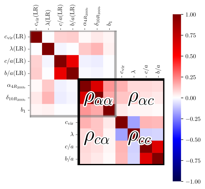
Figure 1: Correlation matrices for the properties of haloes with the lowest masses considered here, $5\cdot 10^{11}<{\rm M_{h}}({\rm M}_{\odot}h^{-1})<7\cdot 10^{11}$. The low resolution (LR) simulation matrix is at the top, outlined in grey, and the high resolution (HR) one, is at the bottom outlined in black. Note that both simulations share the same environmental properties. Each matrix element is colour coded with the value of the Spearman rank correlation value, from $-1$ to $1$, as indicated in the colour bar. We distinguish between intrinsic halo properties, $\@vec{c}=\{c_{vir},\lambda,c/a,b/a\}$, and environmental ones, $\@vec{\alpha}=\{b_{1},\alpha_{4R},\delta_{10R}\}$. We can understand these correlations matrices as being composed of four blocks (eq:blockmatrix): correlations between environmental properties, $\@tens{\rho_{\@vec{\alpha}\@vec{\alpha}}}$; correlations between intrinsic and environmental properties, $\@tens{\rho}_{\@vec{\alpha}\@vec{c}}$ and $\@tens{\rho}_{\@vec{c}\@vec{\alpha}}$; and correlations between intrinsic halo properties, $\@tens{\rho}_{\@vec{c}\@vec{c}}$. Correlations between different halo properties are affected by resolution effects, as can be seen by comparing the top LR matrix with the bottom HR one. The key idea of our method is to incorporate the missing correlations, e.g., the shades of blue indicating negative correlations present in the HR (bottom) but missing in the LR (top).

3 Methods: haloscope

We aim to develop a method to improve the unresolved properties of simulated dark matter haloes. This is important because larger than 90% number of the haloes are unresolved (See Appendix A). We have developed haloscope, a machine learning (ML) technique that uses multi-variate Gaussian distributions with conditional probability given halo properties. Our aims are to i) impose halo property correlations; and ii) make an adequate choice of training parameters to preserve the multi-dimensional assembly bias.

The information we want to predict accurately is the target vector. This comprises of various secondary structural and dynamic properties, $\@vec{c}=\{c_{1},c_{2},..c_{r}\}$. We train the secondary properties with a different ML algorithm introduced in this paper. We also show in Appendix C.2 low mass training with Random Forests and its check consistency with our current method.

We use two types of information for the input feature vector (the input information).

1. A set of features describing the local density field around the halo $\@vec{\alpha}=\{\alpha_{1},\alpha_{2},...\alpha_{q}\}$ , this is defined at a larger scale than the halo and hence sufficiently resolved by the LR simulation.

2. The low-resolution version of the mass and halo properties. These are inaccurate but can be used as a starting point towards more accurate measurement. We later see that this is not important for the recovery of the secondary properties.

Here we generalise the method described in (Ramakrishnan et al. 2021) to the multivariate case we take a vector of $r$ halo properties $\@vec{c}=\{c_{1},c_{2}...c_{r}\}$ and define a vector of $q$ environment variables $\@vec{\alpha}=\{\alpha_{1},\alpha_{2},...\alpha_{q}\}$ together they span a $(r+q)$ - dimensional Gaussian distribution.

$$\begin{bmatrix}\@vec{c}\\ \@vec{\alpha}\end{bmatrix}\sim\mathcal{N}\left(\begin{bmatrix}\@vec{\mu}_{\@vec{c}}\\ \@vec{\mu}_{\@vec{\alpha}}\end{bmatrix},\begin{bmatrix}\@tens{\sigma}_{\@vec{c}}\@tens{\rho}_{\@vec{c}\@vec{c}}\@tens{\sigma}_{\@vec{c}}&\@tens{\sigma}_{\@vec{c}}\@tens{\rho}_{\@vec{c}\@vec{\alpha}}\@tens{\sigma}_{\@vec{\alpha}}\\ \@tens{\sigma}_{\@vec{\alpha}}\@tens{\rho}_{\@vec{\alpha}\@vec{c}}\@tens{\sigma}_{\@vec{c}}&\@tens{\sigma}_{\@vec{\alpha}}\@tens{\rho}_{\@vec{\alpha}\@vec{\alpha}}\@tens{\sigma}_{\@vec{\alpha}}\end{bmatrix}\right)$$ (3)

$\@tens{\sigma}_{\@vec{c}}={\rm diag}(\sigma_{c_{1}},\sigma_{c_{2}},...\sigma_{c_{r}})$ and $\@tens{\sigma}_{\@vec{\alpha}}={\rm diag}(\sigma_{\alpha_{1}},\sigma_{\alpha_{2}},...\sigma_{\alpha_{q}})$ are the block matrices whose elements are the standard deviation of each property, $\@tens{\rho}_{\@vec{c}\@vec{c}}=[{\rho_{c_{i}c_{j}}}$] is the block matrix of correlation coefficients between the different halo properties, $\@tens{\rho}_{\@vec{\alpha}\@vec{\alpha}}=[{\rho_{\alpha_{i}\alpha_{j}}}$] is the block matrix of correlation coefficients between the different environment variables, $\@tens{\rho}_{\@vec{c}\@vec{\alpha}}=[{\rho_{c_{i}\alpha_{j}}}$] is the block matrix of cross-correlations between the halo properties and the environment.

We can visualise these block correlation matrices with examples from N-body simulations as shown in Figure 1. We take 4 halo properties to denote $\@vec{c}=\{c_{vir},\lambda,c/a,b/a\}$ and 3 halo environmental properties to denote $\@vec{\alpha}=\{b_{1},\alpha_{4R},\delta_{10R}\}$. We then compute the block diagonal elements i.e., $\@tens{\rho}_{\@vec{\alpha}\@vec{\alpha}}$, $\@tens{\rho}_{\@vec{\alpha}\@vec{c}}$, $\@tens{\rho}_{\@vec{c}\@vec{c}}$ shown in equation 3 for a well- resolved simulations (demarcated with black border). Such correlations between halo properties have been studied previously e.g., Shin & Diemer (2023). We also show a similar matrix for simulations having poor resolution (top-left and demarcated with grey border). It is very easy to visually see that several correlations exist in the HR haloes are missing in the LR counterparts. Notably,

• comparing the presence and absence of shades of blue in $\@tens{\rho_{\@vec{c}\@vec{c}}}$ for high and low resolutions respectively, indicates that several negative correlations between halo spin and other properties like concentration are absent in the low-resolution.

• the $\@tens{\rho_{\@vec{c}\@vec{\alpha}}}$ in the low resolutions has more white shades and less red while the high resolution has stronger shades of red, this indicates that the halo loses correlations with the environment (assembly bias) in the low resolution.

Our model essentially aims to preserve these correlations when applied to a low-resolution or fast simulation. Since $\@tens{\rho_{\@vec{\alpha}\@vec{\alpha}}}$ is an intermediate-scale property, it is well-resolved in both low and high-resolutions and hence shown just once as a common overlapping region for both high and low resolutions in Figure 1.

In this setup, our model prediction for the distribution of $\@vec{c}$ given $\@vec{\alpha}$, $\@vec{c}|\@vec{\alpha}$, is given by conditional distribution $p(\@vec{c}|\@vec{\alpha})$ which is also another p-dimensional Gaussian distribution i.e.,

$$\@vec{c}|\@vec{\alpha} \sim\mathcal{N}({\@vec{\bar{\mu}}},\@tens{\bar{\Sigma}})$$ (4)

where

$${\@vec{\bar{\mu}}} =\@vec{\mu}_{\@vec{c}}+\@tens{\sigma}_{\@vec{c}}\@tens{\rho}_{\@vec{c}\@vec{\alpha}}\@tens{\rho}^{-1}_{{\@vec{\alpha}}{\@vec{\alpha}}}\@tens{\sigma}^{-1}_{\@vec{\alpha}}(\@vec{\alpha}-\@vec{\mu_{\@vec{\alpha}}})$$ (5)

$$\@vec{\bar{\Sigma}} =\@tens{\sigma_{\@vec{c}}}(\@tens{\rho_{\@vec{c}\@vec{c}}}-\@tens{\rho_{\@vec{c}\@vec{\alpha}}}\@tens{\rho}^{-1}_{\@vec{\alpha}\@vec{\alpha}}\@tens{\rho_{\@vec{\alpha}\@vec{c}}})\@tens{\sigma}_{\@vec{c}}$$ (6)

This is a probabilistic prediction, the scatter $\@tens{\bar{\Sigma}}$ introduces uncertainity in the deterministic linear regression model given by $\@vec{\bar{\mu}}$.

It can be seen from the following that the mathematical framework presented here is a straightforward generalisation of our previous work. In the case where $c$ and $\alpha$ are scalars, in the above equations become $\@tens{\rho_{{\@vec{\alpha}}{\@vec{\alpha}}}}=1$, $\@tens{\rho_{\@vec{c}\@vec{c}}}=1$ and redefining $\@tens{\rho_{\@vec{c}\@vec{\alpha}}}=\rho_{c}$ and standardizing $\tilde{\alpha}=(\alpha-\mu_{\alpha})\sigma^{-1}_{\alpha}$ reduces the above expression to the form familiar from equation 4 in Ramakrishnan & Velmani (2022), i.e.,

$$\bar{{\mu}} ={\mu}_{{c}}+{\sigma}_{{c}}{\rho}_{{c}}\tilde{\alpha}$$ (7)

$${\bar{\Sigma}} ={\sigma^{2}_{c}}(1-{\rho^{2}_{c}})$$ (8)

$$p(c|\tilde{\alpha}) =\dfrac{e^{-(c-\sigma_{c}\rho_{c}\tilde{\alpha}-\mu_{c})^{2}/2\sigma^{2}_{c}(1-\rho^{2}_{c})}}{\sqrt{2\pi\sigma^{2}_{c}(1-\rho^{2}_{c})}}$$ (9)

We also note that this framework is similar to MultiCAM-with scatter (Mendoza et al. 2023) and KLLR (Farahi et al. 2022), demonstrating the scope of applications to other problems in astronomy and cosmology. While we target large-volume simulations and aim to improve the low-resolution halo properties and their assembly bias given the information about the present-day local environment, Mendoza et al. (2023) introduces a generalisation of the conditional abundance matching technique (Hearin & Watson 2013) and uses the same formalism for predicting the present-day halo properties given the accretion history of the halo traced back in time.

Throughout this discussion the halo mass dependence is suppressed for brevity, it is to be noted that we refit our model in bins of different mass ranges.

3.0.1 Gaussianisation of Variables

The above formalism relies on the assumption that both the feature and target variables are Gaussian when in reality they have skewed distributions. Hence, all the variables need to be transformed to have a Gaussian distribution before applying the algorithm and inverse-transformed to their original distributions. In our previous paper, we applied different transformations tailored to the distribution of each specific halo or environment property. For eg., a Logarithmic transformation works fairly well to Gaussianize halo concentration and halo spin. However, this approach requires us to know an analytical description of the distribution to make an informed choice as to what transformation to apply in each case.

To overcome this, here we use instead the sci-kit-learn implementation called quantile transformer. This is based on multivariate probability integral transform (Rosenblatt 1952) that has two advantages — it can Gaussianize any arbitrary distribution and it preserves rank correlations between the variables.

3.0.2 Linear Constraints

The sampling of a multivariate Gaussian distribution that ignores the linear inequality constraints inherent in halo properties, specifically

$$c_{\rm vir} >0,$$ (10)

$$\lambda >0,$$

$$c/a >0,$$

$$b/a-c/a >0$$

$$1-b/a >0$$

We address this issue by using a rejection sampling algorithm that discards samples that fail to adhere to these constraints. For our problem, rejection sampling has an acceptance rate greater than 96% for all the mass ranges considered, hence practical and efficient. We note that alternative methodologies for sampling a truncated Gaussian are available in the existing literature, owing to the ubiquity of such challenges in statistical applications.

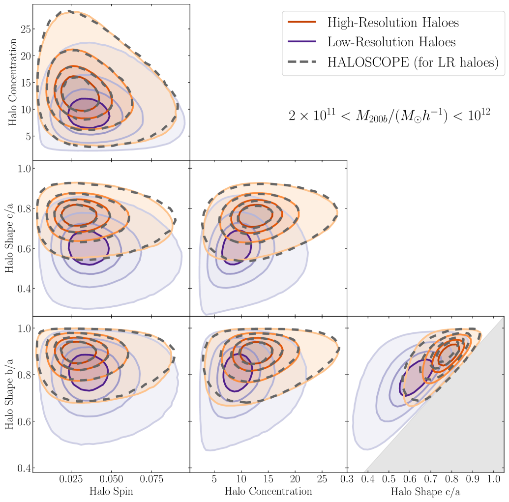
Figure 2: Confidence intervals (20%, 40%, 68% and 95% ) for the distribution of pairs of properties of haloes with $2\times 10^{11}<M_{200b}(M_{\odot}h^{-1})<10^{12}$, corresponding to haloes having from $20$ to $100$ particles in the LR simulation. In the bottom right panel the grey area simply indicates a forbidden region, due to the constraint $a>b>c$. Blue contours show the distribution of LR haloes, while the orange ones show that for the HR haloes. The dashed black contours represent the new distribution of the LR haloes after applying haloscope. Our algorithm is able to recover the bivariate distribution of LR halo properties.

4 haloscope applied to a low-resolution simulation

In this work, we use haloscope to enhance the properties (concentration, spin and two shape parameters) of unresolved dark matter haloes in a low-resolution (LR) simulation, given an eight times higher resolution (HR) one. By construction, the method is designed to recover the mean halo property relation with halo mass and its scatter (See Appendix E for this discussion). Besides this we are also interested in recovering the multi-dimensional distribution at every mass range. This will allow us to capture the self-correlations between halo properties, e.g., the blue shades present in the HR correlation matrix but absent in the LR correlation matrix in Figure 1 show the absence of anti-correlation between halo spin and various halo properties. Missing out on such correlations can impact galaxy formation models,e.g., Posti et al. (2020) shows how residuals in galaxy scaling laws are sensitive to the anti-correlation between the spin and concentration and Zhang et al. (2023) models the correlations between halo properties to address systematics in galaxy cluster cosmology with weak lensing scaling relations.

We use the algorithm we have developed, haloscope, to create a model halo catalogue of halo properties in the LR simulation. Thus the low-resolution haloes have two sets of halo properties, one computed with the halo finder and the other using our algorithm, we compare these with high-resolution haloes computed with a halo finder.

In Figure 2, in each panel, the bivariate distribution of a pair of halo properties is shown using the 20%, 40%, 68% and 95% confidence contours. The orange contours which show the high-resolution distribution can be distinctly distinguished from the blue contours which show the low-resolution distribution. In each case, the center of the LR contour drops in value compared to the HR contour for all the halo properties except those involving spin where there is rise in the value along the relevant axis, these numerical convergence trends can also be seen in the median relation at the lowest halo mass bin in Fig. 11. Further, the shape of the LR contours are also different – more spherical and less tilted – than the shape of the HR contours. Finally, the grey dashed lines in each panel shows the distribution of halo properties from haloscope on the low-resolution haloes, we can see remarkable agreement with the contours of the high-resolution haloes. The non-Gaussian shapes are also recovered because of our method’s final step of using a quantile transformer (see the goodness of fit in sec:KS).

Figure 12 shows mass dependence of the bivariate distribution between concentration and spin, as the halo mass increases all three contours begin to overlap as expected.(More details in Appendix  12). Although not shown here, we also obtain similar results for all other bivariate distributions with other halo properties.

Figure  11 looks at the trend in the median value of the halo properties at any given halo mass. At high masses, there are no differences between the three different halo catalogues because all haloes are well resolved. At low masses, there are deviations in the median value of any halo property computed using the halo finder for the high resolution (orange line) and the low resolution (purple line). The predicted halo properties from haloscope (dashed lines) on the low-resolution haloes has a better match with the high-resolution halo properties.

5 Recovering Multi-dimensional Halo Assembly bias

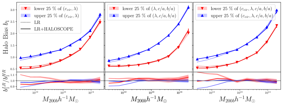
Figure 3: Top panels: the linear halo bias as a function of halo mass for split populations of haloes, to show the assembly bias signal. In blue (red) is shown the linear bias of the upper (lower) $25$% of haloes according to: concentration and spin in the left panel; spin and two shape parameters in the middle panel; and concentration, spin and two shape parameters in the right panel. Triangles show the HR haloes, dashed lines the LR ones and the thick continuous lines are the result of applying haloscope to the LR haloes, LR$+$haloscope. Shaded regions correspond to the standard error on the mean. Bottom panels: the LR and LR$+$haloscope results divided by the HR ones. Our algorithm is capable of recovering the multi-dimensional halo assembly bias measured in HR simulations from the LR haloes.

Since cosmological survey analyses largely rely on clustering statistics, it is of paramount importance for any model catalogue to preserve its correlations with the local density environment. In the case of dark matter halo properties such as dependence on the environment at fixed halo mass is called halo assembly bias and has been widely studied in the literature. The halo assembly bias coupled with a beyond-mass halo occupation distribution (HOD) consequently results in an effect in galaxy distribution called the galaxy assembly bias.

The strength and shape of the halo assembly bias vary depending on the halo properties and mass range under consideration. Studies on halo assembly bias mostly look at one halo property at a time for e.g.(Faltenbacher & White 2010), It would be interesting to look at the differences in halo bias for similar halo mass but different sub-populations demarcated in the multi-dimensional distribution of halo properties shown in Figure 2– we can call this multi-dimensional assembly bias. Some examples of previous such studies are from Lazeyras et al. (2017) that looks at halo assembly bias with pair of properties simultaneously and Montero-Dorta & Rodriguez (2023) that looks at galaxy assembly bias with multiple properties.

In Figure 3, the blue and red markers show how the halo assembly bias looks like with respect to the different combinations of halo properties. In the left panel, the red triangular markers show, at every mass bin, the halo bias of the lower 25% of $(c_{vir},\lambda)$ which is a population of haloes below the $p^{th}$ percentile in both $c_{vir}$ and $\lambda$ and the blue markers show the halo bias of the upper 25% of $(c_{vir},\lambda)$ which is a population above $100-p^{th}$ percentile. Under such segregation, there is a gap between the linear bias in the two populations, and the gap does not invert like seen while segregating with halo concentration alone. Instead, the gap steadily decreases with halo mass.

In the middle panel, we consider linear halo bias, at fixed mass, between two populations segregated according to a combination of three halo properties following a similar procedure as before to obtain the linear bias of upper 25% in $(\lambda,c/a,b/a)$ shown with blue markers and the lower 25% of $(\lambda,c/a,b/a)$ shown with red markers. Interestingly, the trend with mass is opposite from before, the gap between the linear bias in the two populations increases with increasing halo mass.

Finally, in the right panel, we compare two populations made of a combination of all 4 of the halo properties i.e, the upper 25% of $(c_{vir},\lambda,c/a,b/a)$ shown again in blue markers and the lower 25% of $(c_{vir},\lambda,c/a,b/a)$ shown with red markers, the gap in the linear bias between these two populations at every halo mass is fairly constant.

The combinations in each panel of fig:ab were chosen to demonstrate that the trend of the assembly bias signal with the halo mass could decrease, increase or remain fairly constant throughout the mass range considered. Other arbitrary combinations of halo properties have also been verified but not shown here. Secondary dependence on the clustering signal beyond halo mass is dependent on multiple different properties with various trends at different halo masses.

In the way we have trained our model, we recover the halo assembly bias since it predicts halo properties $\@vec{c}$ given the nature of the environment $\@vec{\alpha}$ (eq:model). Moreover, we use the tidal anisotropy or $\alpha_{4R}$ as one of the input environmental parameters which has to be shown to be the primary indicator for halo assembly bias with respect to multiple halo properties (Ramakrishnan et al. 2019).

The solid lines in each of the top panel of Fig. 3 show assembly bias in the halo properties predicted by our model firstly agrees qualitatively well with the expected behavior shown by markers, and quantitatively within few percent of the high resolution as seen in the ratio of the two in bottom sub-panels. It is also remarkable that trends in the halo assembly bias with respect to any combinations of halo properties are recovered at all the mass ranges considered. This has particularly useful applications for fast approximate simulations/catalogues (Feng et al. 2016; Balaguera-Antolínez et al. 2019) that do not contain halo assembly bias but contain sufficient information regarding the halo mass and tidal environment which are the only primary inputs to our model (See Appendix G for a study of feature importance of the inputs). Our halo catalogues also have improved upon the results with low-resolution haloes shown in dashed lines in Figure 3, the agreement with high resolution is within 10% for the low-resolution haloes while it is within 5% agreement for our model. The improvements are especially for low-mass haloes (20-500 particles) which constitute more than 90% of the total haloes (See Figure 6).

6 Effect of halo properties on galaxy clustering

In this section, we show the effect that improving halo properties with haloscope has on the clustering of central galaxies. We choose to focus solely on central galaxies to reduce the number of free parameters in the halo occupation distribution (HOD) model used to populate with galaxies the unit simulation. This choice allow us to get a cleaner view of the effect of haloscope in the galaxy clustering at large scales. We defer to future works a detail study of satellite galaxies.

6.1 Model galaxy catalogues

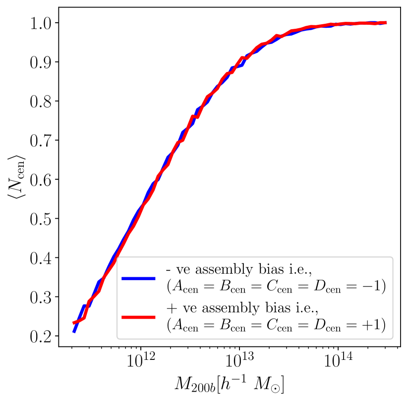
Figure 4: Average number of central galaxies as a function of halo mass for catalogues generated using two different assembly bias models (Equations 11 and  12). We have pairs of catalogues of central galaxies hosted by haloes with similar mass distributions but different concentrations, spins and shapes.

,

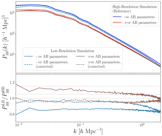
Figure 5: Top panel: power spectrum for model galaxies. Catalogues produced with a positive assembly bias (eq:gab), +ve AB with $A_{\rm cen}=B_{\rm cen}=C_{\rm cen}=D_{\rm cen}=1$, are shown in red, and those with a negative one, -ve AB, in blue, $A_{\rm cen}=B_{\rm cen}=C_{\rm cen}=D_{\rm cen}=-1$. Continuous brighter lines show the results for galaxies generated on the HR simulation, while continuous lines with darker colours correspond to the LR simulation. The dashed lines show those catalogues generated on haloes from the LR simulation after applying haloscope (corrected, LH$+$haloscope). There are differences ranging from 50 to 20 % in the power spectrum between the +ve AB and -ve AB catalogues for the range of k modes. This is due to the galaxy assembly bias, as the two sets of catalogues have similar average halo occupation distributions (see Figure 4). Bottom panel: Ratios with respect to the galaxy catalogues from the HR simulation of both the LR (solid brown and light-blue lines) and LH$+$haloscope, or corrected dark matter haloes (dashed brown and light-blue lines). Horizontal grey lines indicate the $0$, $5$ and $15$ per cent levels. The ratios of power spectrum from two tracers of the same field cancel the statistical noise, that it was already reduced thanks to the fixed-pair method used in the unit simulations (more details in section 6.2) There are $15$% differences between the power spectrum of HR and LR galaxy catalogues. Our algorithm, can reduce this difference to $5$%.

We use a HOD model to populate with central galaxies the dark matter haloes of both HR and LR simulations. We then study the central galaxies clustering for the same set of HOD parameters. The continuous expansion in capabilities of cosmological surveys, such as DESI (DESI Collaboration et al. 2024) and Euclid (Euclid Collaboration et al. 2024a), have created a demand for simulations that are larger in volume and more accurate at smaller scales. Faced with the computational costs of such simulations, to incorporate cosmological tracers in them, we often need resort to connecting galaxies to haloes using computationally effective tools such as the HOD models.

For the average occupancy of central galaxies in haloes of a given mass, $\langle N_{\rm cen}\rangle$, we use the following standard form (e.g. Zheng et al. 2005; Reyes-Peraza et al. 2024):

$$\langle N_{\rm cen}\rangle=1/2\left(1+\mathrm{erf}\dfrac{(\log M_{h}-\log M_{\rm min})}{\sigma_{\log M}}\right)$$ (11)

We choose $\log M_{min}=11.95$ and $\sigma_{\log M}=0.65$ for our baseline model. This implies that $\langle N_{cen}\rangle$ transition from $0$ to $1$ in a mass range centered in $\log M_{min}=11.95$, as it can be seen in fig:hod. For our LR simulation, this value corresponds to few tens to hundreds of particles per halo thus making it an ideal choice of parameters for our specific study.

In addition, we also model the assembly bias signal by altering $\log M_{min}$ in the following way,

$$\log M_{min}^{\prime}=\log M_{min}+A_{cen}f_{a}+B_{cen}f_{b}+C_{cen}f_{c}+D_{cen}f_{d}\,$$ (12)

where $f_{a},f_{b},f_{c},f_{d}$ are rank of halo the four properties ($a$,$b$,$c$ and $d$) for every mass range. The rank has been normalised to range between -0.5 to 0.5. $A_{cen},B_{cen},C_{cen},D_{cen}$ are the assembly bias parameters. In the following exercise we will choose two sets of assembly bias parameters, the negative set i.e,($A_{cen}=B_{cen}=C_{cen}=D_{cen}=-1$) and the positive set i.e., ($A_{cen}=B_{cen}=C_{cen}=D_{cen}=1$). The reason to choose the above sets of parameters is simply to explore the extreme scenarios or the boundary of the priors. This also gives a conservative estimate of the amount of systematics that can be induced by resolution effects in a simulation.

We have produced three pairs of galaxy catalogues, based on either the HR, LR or the LR$+$haloscope haloes. For each pair of catalogues, we have one with the negative set of assembly bias parameters (-ve AB) and the other with the positive set of assembly bias parameters (+ve AB). Figure 4 shows the how the halo occupation distribution of the central galaxies is similar for the catalogues with -ve AB and +ve AB, we can find same results in the other catalogs also. The difference between the two populations occurs in how the secondary halo properties are preferentially populated in the central galaxy population, while the negative set of assembly bias parameters preferentially chooses to populate central galaxies in more concentrated, larger spin and ellipsoidal shapes, the negative set of assembly bias parameters preferentially populates spherical, less concentrated and less spin haloes with central galaxies.

6.2 Clustering of model galaxies

We measure the power spectrum of the six galaxy catalogues we have generated in pairs of +ve AB and -ve AB. The host haloes come from the HR and LR simulations. We have also applied haloscope to the LR simulation, LR$+$haloscope, to enhance the input halo properties.

There are $\sim 50-20$% differences in the power spectrum for the range of k modes, when comparing the power spectrum measured for the pairs of catalogues with a positive and a negative assembly bias (top panel in fig:galaxyps). This result is independent of the input host haloes. We find that the halo assembly bias directly propagates into the galaxy assembly bias i.e, the central galaxies from the +ve AB and -ve AB catalogues have similar average HODs (fig:hod), but $\sim$40% differences in their power spectrum (blue and red lines in the top panel of fig:galaxyps).

Next, we compare the differences between the LR and HR galaxy catalogs having identical HOD prescriptions. The power spectrum from the LR galaxy catalogues differs by 15% from the HR version of the same halo-galaxy (solid lines in the bottom panel of fig:galaxyps). The differences seen in clustering between the HR and LR catalogues may possibly be absorbed into a different set of HOD parameters, but our analysis indicates that one has to be cautious while transferring HOD calibrations obtained from one resolution to use onto another one.

We finally apply haloscope on the LR simulations and compare the galaxy catalog with the HR counterpart. The power spectrum of the catalogues generated from the haloes derived applying haloscope to the LR simulation, is within $5$% of the HR one. Our method manages to reduce the previous discrepancy of 15 % to 5% (bottom panel in fig:galaxyps). It is to be noted that the differences between the LR and HR model catalogues have a reduced cosmic variance because of the fixed-pair technique used to generate initial conditions for the unit simulations (Angulo & Pontzen 2016). Moreover, the LR and HR sets of the unit simulations have identical initial phases, i.e., they trace the same large-scale density field, so taking ratios is designed to cancel the statistical fluctuation errors (McDonald & Seljak 2009).

At small scales ($k>0.6hMpc^{-1}$), the agreement with the HR reduces back to what is expected for LR haloes by $k=2hMpc^{-1}$ which seems to be a limitation of our method.

Currently, many HOD prescriptions address the resolution issue by simply sampling from a fitting function such as a concentration-mass relation in the poorly resolved regime, and rank order/rearrange the samples to abundance match with the existing poor resolution sample (Paranjape et al. 2021; Euclid Collaboration et al. 2024a). While such a method corrects for the value of the halo properties and incorporates assembly bias to the levels expected in a LR simulation, we would like to emphasise that the analysis here shows the problems that exist beyond such a correction at larger scales that simply involves the ranks and not the actual value of the halo properties.

The improvement in the clustering once we have applied haloscope demonstrates the utility of our method to enhance summary statistics for model galaxies based on low resolution simulations.

7 Summary and conclusions

We have developed a machine learning method, haloscope (sec:method), to improve unresolved properties of dark matter haloes in simulations, while preserving the multi-dimensional assembly bias. The code associated with this method is publicly available.

The success of the method is demonstrated by accessing low-mass - poorly resolved haloes in a large-volume simulation and correcting for their halo properties to produce results similar to haloes that have achieved numerical convergence. In particular, we have tested haloscope using the original unit simulation (Chuang et al. 2019), referred here as the high-resolution (HR) simulation, and a simulation with eight times worse resolution, the lower-resolution (LR) simulation (sec:sim). For the application presented here, we aim to recover the properties of the HR haloes. Our method is trained using halo properties in bins of halo mass.

By training haloscope with HR halo properties and then applying it to LR haloes, LR$+$haloscope, we can conclude the following:

• haloscope has been developed to recover the distributions and correlations of halo properties in halo mass bins (Figures 2 and 12). Our algorithm also recovers the median and scatter expected for the distribution of halo properties as a function of halo mass (fig:prelimresult).

• haloscope can recover, for the first time, the multi-dimensional halo assembly bias (fig:ab), i.e., the dependence of halo bias simultaneously on arbitrary combinations of the halo properties at a fixed mass. This is only possible when environmental properties, such as the linear bias and the tidal anisotropy (see sec:env) are used in the training of haloscope (fig:contributions). LR$+$haloscope reduces the differences in multi-dimensional assembly bias between HR and LR from 12% to 5% .

This new method is particularly useful in the lowest mass range where there are significant differences between the LR and HR simulations. This is due to the large amount of unresolved properties for low-mass haloes in the LR simulation. We have tested that our method and the conclusions above are robust against different definitions of halo mass (sec:alternatemass). Our algorithm can also be applied after improving the halo mass function using different machine learning algorithms, such as random forest. However this improvement provides very small changes to the halo mass, that cannot improve the unresolved properties of haloes, at least for the case under study (sec:improve_mass).

The clustering of model galaxies can be affected by that of their host haloes. We have studied this by generating catalogues of galaxies with a halo occupation distribution (HOD) model, including assembly bias. We have produced catalogues of central galaxies based on the HR, LR and LR$+$haloscope haloes. We focus on central galaxies to be able to limit the free parameters of the HOD model. We have used two extreme HOD models, one with a positive assembly bias, +ve AB, and an other with a negative one, -ve AB (see eq:gab). Studying the power spectrum of the six galaxy catalogues we conclude the following:

• The galaxy assembly bias is directly affected by the halo assembly bias. The power spectrum is up to $50$-20% (depending on the k mode) different between the +ve AB and -ve AB galaxy catalogues (fig:galaxyps). This difference in clustering occurs despite having similar average occupancies with halo mass (fig:hod).

• haloscope improves the central galaxy power spectrum with respect to the HR catalogue (for $k<0.6h^{-1}Mpc$), by going from a $15$% difference with the LR catalgoue to a $5$% difference for the LR$+$haloscope (fig:galaxyps).

In this work we have focused on enhancing the low-resolution halo properties. However, other applications are possible. Fast approaches to numerical simulations (Scoccimarro & Sheth 2002; Monaco et al. 2002; Avila et al. 2015; Balaguera-Antolínez et al. 2019) can now be enhanced with haloscope to preserve the multi-dimensional assembly bias found in full numerical simulation. This is possible because haloscope only requires the large-scale structures and tidal environment as input. This is a very promising application, as internal halo properties are unavailable for the entire dynamic range of the approximate gravity solvers as has been demonstrated by Balaguera-Antolinez & Montero-Dorta (2024). haloscope has also the potential to be used to recover the effect that baryons have on dark matter haloes and, possibly, connecting directly galaxies to haloes. This work highlights the potential of machine learning methods to recover missing small-scale physics in simulations that are limited by resolution.

Appendix A Percentage of haloes with unresolved properties

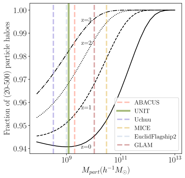
Figure 6: Fraction of the total haloes in a simulation formed by 20 to 500 particles, as a function of the particle resolution, $M_{\rm part}$, of a simulation. This fraction has been calculated using the Tinker et al. (2008) halo mass function with Planck-18 cosmological parameters (Planck Collaboration et al. 2020) and varies for different redshifts (see labels in the Figure). The vertical dashed lines of different colours indicate the location of state-of-the-art simulations, as indicated in the legend. The green solid vertical corresponds to unit, the simulation used in this work (sec:sim). Over 90% of the haloes in these simulations have unresolved halo properties and this number increases for higher redshifts.

Over 90% of dark matter haloes in simulations are unresolved, i.e., they do not have converged halo properties (see Figure 6). The numerical resolution of an N-body simulation sets a limit to the smallest mass of the dark matter halo that can be resolved. Typically, a halo requires few tens to hundreds of particles to for its mass to be well resolved. However, most of the secondary beyond-mass halo properties require at least few hundreds to thousand particles to be fully resolved (Mansfield & Avestruz 2021). As the halo mass function decreases rapidly with mass, most of the haloes in a simulation are low mass and thus unresolved. Figure 6 shows the fraction of low mass haloes comprising of 20-500 particles as a function of the particle resolution of a simulation. To provide a more realistic view of the problem, we also show in the same figure, state-of-the-art simulations from which galaxy catalogues have been produced.

Appendix B Smoothing scale for the tidal anisotropy

In this section, we provide a self-contained reasoning for the choice of $4\times R_{200b}$ to describe the tidal anisotropy around a halo. We compute $\alpha_{S}$ for several Gaussian smoothing scales ranging from [0.24,4] $h^{-1}Mpc$ and measure its rank correlation with $\delta_{S}$. In Figure 7 this rank correlation is plotted as a function of the halo mass, we can see that the rank correlation peaks at different halo masses for different scales, the correlations with smaller smoothing scale peaking for smaller masses and the correlations with larger smoothing scale peaking at higher masses. The black line corresponds to the rank correlation $\rho_{\alpha-\delta}$ at a variable smoothing scale corresponding to 4 $\times$ halo radius. Comparing the black line which forms an envelope around the other coloured lines, it becomes apparent the peak in rank correlation at any fixed scale is identical to 4 times the radius for that halo mass bin. Since we are interested to maximimally recover the correlations with the large scale clustering environment $\alpha_{4R200b}$ becomes the obvious choice as input parameters in our algorithm as opposed to fixed smoothing scales.

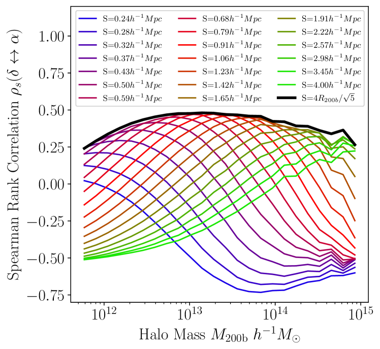
Figure 7: Spearman rank correlation between the tidal anisotropy and the overdensity as a function of halo mass. Different fixed Gaussian smoothing scales, $S$, have been used, as indicated by the legend. The black solid line indicates the Spearman rank correlation at a variable scale corresponding to the radius of the halo, i.e., $4\cdot R_{200b}/\sqrt{5}$. Our chosen smoothing scale for the tidal anisotropy, $4\cdot R_{200b}$, corresponds to the maximum correlation for any mass range considered envelopes the others.

Appendix C Halo masses

C.1 Alternative mass definitions

Figure 8 explores how the three different mass definitions of a halo are correlated to each other. The mass definitions that we use are $M_{\rm 200b}$ which is the mass enclosed inside 200 $\times$ the background density, $M_{\rm 200c}$ which is the mass enclosed inside 200 $\times$ the critical density and $V_{\rm peak}$ which is the peak circular velocity over the accretion history of a halo. We see tight correlation between the three definitions.

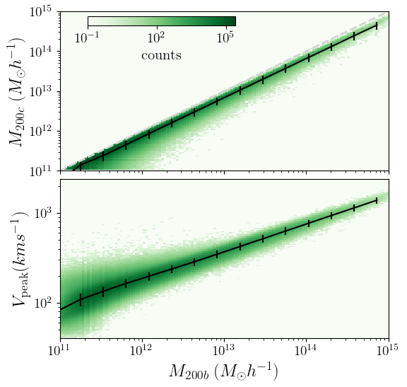
Figure 8: Correlation between $M_{200b}$ and $M_{200c}$, top panel, and $V_{peak}$, bottom panel. Black lines show the median and standard deviation. The number of haloes are shown as coloured regions, following the colour bar. The dashed grey line shows the one-to-one relation. All definitions of the halo mass are highly correlated, although there is substantial scatter in the case of $V_{peak}$.

C.2 Improving the low mass HMF

The primary property of a dark matter halo is its mass. In simulations, there are several definitions and proxies for the mass of the halo due to the lack of consensus on a well-defined halo boundary. The convergence in halo mass is generally much better than the other secondary properties, while the secondary properties require a few hundred particles for convergence, mass convergence can be achieved at a few tens of particles. Yet further improvements in the halo mass function are desirable since model catalogues for large-scale surveys seek to maximise the dynamic range offered by a simulation (Armijo et al. 2022; Angulo et al. 2014). Here we improve the mass function by applying the mass correction method in Forero-Sánchez et al. (2022) and subsequently apply haloscope to test the validity of our algorithm. We follow the hyperparameters for the training algorithm as prescribed in their work, except for the number of estimators which is set to one. The other difference is that they use haloes from subfind while we use rockstar haloes. Figure 9 shows the halo mass function in HR and LR simulations in orange and purple solid lines. From the ratio of the two mass functions shown in green in the bottom panel, we can see that the mass function converges to sub-percent accuracy at high masses. However, due to numerical resolution effects the halo number density drops from the expected value by 10 percent for 40 particle haloes. After correcting for the masses based on the 1-1 matching and training the data set with a RF algorithm some of the LR haloes at the low mass end are matched with higher mass HR haloes. This increases the halo counts at higher masses happens at the cost of losing haloes below the 40-particle mark, thus increasing the completeness of the halo catalogue at higher masses. We also check for 1-1 matching with alternative mass definition in Appendix 9. We had also experimented with alternate methods such as XGboost, NGboost and concluded that they do not bring about much changes than the current method.

Figure 9: Halo Mass function: Comparison of halo mass function of the LR simulation (purple solid lines) with the HR simulation (orange solid lines). The mass function of the LR simulation is within $10\%$ of HR simulation for LR haloes greater than 40 particles as can be seen from the solid purple line in the bottom panel. The black dashed line corresponds to the low-resolution haloes after correcting their masses with the high-resolution counterparts with a simple 1-1 matching. After the 1-1 matching, and training with RF, the completeness of the haloes above 40 particle haloes increases but at the cost of lower mass haloes.

In Figure 10, we use an alternative mass definition of $M_{200c}$ to do the 1-1 matching between the HR and LR and subsquent RF training to predict and improve the halo mass function. This excercise demonstrates the robustness of the method to alternate mass definitions.

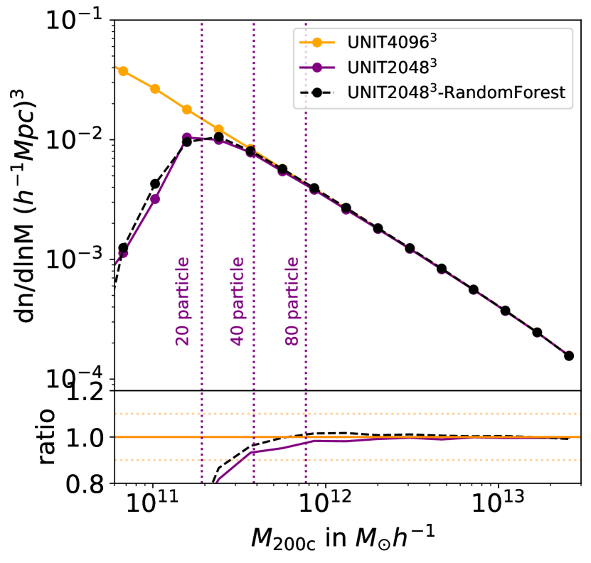
Figure 10: Halo Mass function: Similar to Figure 9 with the difference that $M_{200c}$ has been used to do the 1-1 matching and subsequent RF training. Improvements in the HMF can be seen for haloes above 30 particles.

Appendix D haloscope: Goodness of fit

Here we use the KS test to compare the distribution of the halo properties generated with haloscope with that of the high-resolution simulation. The KS statistic is computed in Table 1 with the null hypothesis that both samples belong to the same distribution. We limited our sample size to 10,000 haloes in each mass range to prevent heightened sensitivity in our statistical tests for large sample sizes and to prevent frequent null hypothesis rejection (Lin et al. 2013).

KS Statistic for 1-D distributions
Halo Mass $M_{\odot}h^{-1}$	$c_{vir}$	$\lambda$	$c/a$	$b/a$
3.0 $\times 10^{11}$	0.012	0.012	0.015	0.023
$6.8\times 10^{11}$	0.012	0.012	0.014	0.025
$1.5\times 10^{12}$	0.012	0.012	0.014	0.026
$3.5\times 10^{12}$	0.01	0.011	0.013	0.027
$7.9\times 10^{12}$	0.011	0.01	0.012	0.027
$1.8\times 10^{13}$	0.01	0.01	0.011	0.022
$4.1\times 10^{13}$	0.009	0.009	0.01	0.019
$9.2\times 10^{13}$	0.008	0.008	0.008	0.015
$2.1\times 10^{14}$	0.008	0.007	0.007	0.005

Table 1: The table reports KS statistic comparing 1-D distributions of the halo properties with the high-resolution simulation. We choose a pvalue $\leq$ 0.001 to reject the null hypothesis which corresponds to a KS statistic $\geq$ 0.0274. We can see all the values reported above are below this threshold. The table indicates good agreement between the distributions of haloscope halo properties and those from the HR simulations.

.

Appendix E haloscope: Recovering the mean and scatter of the halo property at a given halo mass

The numerical convergence problems create an offset in the mean and scatter of the distribution of halo properties at the lowest mass range. Since any method that tries to correct for the halo properties primarily targets accuracy in these two statistics, in Figure 11 we show the accuracy of haloscope in retrieving these statistics.

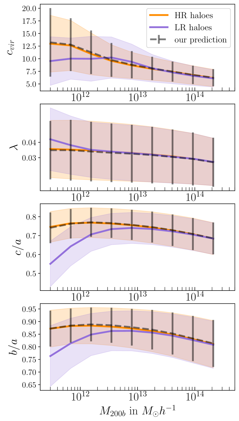
Figure 11: In each panel, we show the median halo property as a function of halo mass for high-resolution (HR) haloes, low-resolution (LR) haloes, and applying haloscope on the low-resolution haloes in black dashed lines. Our method recovers the median and central 69 percentile of the halo property for any halo mass.

Appendix F haloscope for varying mass bins

Figure 12: Same as the top panel of Figure 2 but for different mass bins, up to masses such that haloes will have at least 6000 particles (right panel). The orange contours are for the HR haloes and the blue ones for the LR haloes. Dashed grey contours show the result of applying haloscope to the LR haloes. The differences between HR and LR decrease with halo mass, as halo properties can be resolved when haloes contain a large enough number of particles.

In the main text, we focused on haloes in the lowest mass bin where the halo properties are least converged and demonstrated how applying haloscope can improve the bivariate distribution of halo properties. Here, we show the results for the other mass bins. Figure 12 focuses on the bivariate distribution of halo concentration and halo spin where $\@vec{\bar{\Sigma}}$ and $\@vec{\bar{\mu}}$ in equation 5 and 6 are recomputed for four different mass ranges. Though not shown, we have also verified similar results when varying masses for the bivariate distributions for other combinations of halo properties.

Appendix G haloscope as a function of input parameters

Here we aim to analyze the goodness of fit of our algorithm in relation to every individual input parameter. Such a study helps to understand the feature importance of different inputs. The top panel of Figure 13 shows that there is no assembly bias when random uncorrelated inputs are given. This is analogous to a situation where no inputs are given. Mock catalogs modeled simply with a mean or median concentration-mass relation with scatter would not carry halo assembly bias information similar to the solid lines in the top right panel. In the top middle panel, the low resolution halo properties are used as input and we can see it does not improve the assembly bias at the low mass end. In the top right panel, the input parameter is the halo overdensity is computed at $10R_{\rm 200b}$. In the bottom panel, we have shown the best three cases for recovering halo assembly bias where the input is $\alpha_{4R}$(left panel) halo bias $b_{1}$(middle panel) and $\alpha_{4R}+b_{1}$ in the right panel.

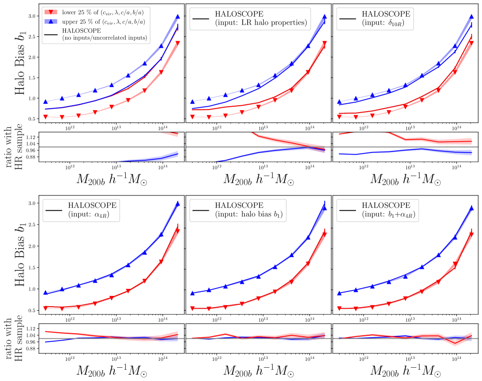
Figure 13: Same as fig:ab, but haloscope has been trained with different input properties. In the top left panel, random uncorrelated inputs are used for training haloscope and when we apply our algorithm to the LR haloes, LR$+$haloscope, no halo assembly bias is measured. In the top middle panel, we train haloscope with properties from LR haloes. For the other panels, haloscope is trained with the HR properties indicated in the legend. In all the panels, the blue and red triangles correspond to the upper and lower $25\%$ of ($c_{vir},\lambda,c/a,b/a$) HR haloes. This is our reference. To recover the multi-dimensional halo assembly bias, haloscope needs to be trained with environmental properties; in particular $b_{1}$, $\alpha_{4R}$ and a combination of the two give the best results.