Renormalons as Saddle Points

Abstract

Instantons and renormalons play important roles at the interface between perturbative and non-perturbative quantum field theory. They are both associated with branch points in the Borel transform of asymptotic series, and as such can be detected in perturbation theory. However, while instantons are associated with non-perturbative saddle points of the path integral, renormalons have mostly been understood in terms of Feynman diagrams and the operator product expansion. We provide a non-perturbative path integral explanation of how both instantons and renormalons produce singularities in the Borel plane using representative finite-dimensional integrals. In particular, renormalons can be understood as saddle points of the 1-loop effective action, enabled by a crucial contribution from the quantum scale anomaly. These results enable an exploration of renormalons from the path integral and thereby provide a new way to probe connections between perturbative and non-perturbative physics in QCD and other theories.

Introduction. The interface between perturbative and non-perturbative physics is at the heart of some of the deepest challenges in quantum field theory. Two objects which allow for quantitative exploration of this interface are instantons and renormalons Lipatov (1977); ’t Hooft (1979); Lautrup (1977). Instantons are semi-classical objects: solutions to the classical (Euclidean) equations of motion of a theory which mediate non-perturbative phenomena, such as tunneling. Renormalons leave a similar imprint on perturbation theory as instantons but have resisted a semi-classical interpretation. Many insights into renormalons have come from 2D models Gross and Neveu (1974); Novikov et al. (1984); Beneke and Zakharov (1993); Mariño and Reis (2020a, b), supersymmetric models Schubring et al. (2021); Shifman (2015, 2023), and models in compactified spacetimes Argyres and Unsal (2012a, b); Dunne and Ünsal (2013); Dunne and Unsal (2012). Infrared (IR) renormalons are particularly important as they associate growth in perturbation theory with the size of power corrections Maiani et al. (1992); Beneke (1999). Practical uses of renormalons include motivating judicious choices of renormalization scheme Grozin and Neubert (1997); Hoang et al. (2010) and heavy quark mass determination Luke et al. (1995); Beneke et al. (2017); Hoang et al. (2018). Because instantons have a semi-classical interpretation, one can reconstruct information about the classical action and corresponding field configurations of instantons from their signature in the Borel plane. Analogously, the Borel transform of a perturbative series containing a renormalon suggests that the renormalon should have an associated action – but the action of what? We answer this question by showing that renormalons correspond to saddle points of the effective action in field theories with anomalous scale invariance.

Our approach is to begin with the more general question of how Borel transforms of asymptotic series encode the ‘actions’ of exponential integrals. For series associated with instantons, we show that in many cases one can fully rebuild the relevant part of the action from the series, which amounts to uncovering its non-perturbative definition. The semi-classical interpretation of renormalons is more subtle and requires consideration of Lefschetz thimble 2-manifolds embedded in $\mathbb{C}^{2}$. By repackaging insights from Morse theory in more physical terms, we explain an effective way to think about the multidimensional case. We first discuss a 2D integral example as a toy model. Then we show that in QCD, by judiciously integrating out degrees of freedom, operator expectation values containing renormalons can be understood with 2D integrals of the form of our toy model. More generally, we argue that for a classically scale-invariant field theory, the activation of the scale anomaly generates an effective action with renormalon saddles which are not present in the bare action.

Action-Borel correspondence. The Borel transform is defined from a series $f(g)=\sum_{n=0}^{\infty}c_{n}g^{n+a}$ by

$$B(t)={\mathcal{B}}[f](t)=\sum_{n=0}^{\infty}\frac{c_{n}}{\Gamma(n+a+1)}\,t^{n+a}\,,$$ (1)

where $a$ can be any number greater than $-1$. We will use the notations $B(t)$ and ${\mathcal{B}}[f](t)$ interchangeably. The corresponding inverse Borel transform is

$${\mathcal{B}}^{-1}[B](g)=\frac{1}{g}\int_{0}^{\infty}dt\ e^{-\frac{t}{g}}B(t)\,,$$ (2)

which formally reproduces the original series order-by-order in $n$. We note that the function $\frac{1}{g}f(g)$ is in obvious 1-to-1 correspondence with $f(g)$; however, its Borel transform is

$${\mathcal{B}}\!\left[\frac{1}{g}f(g)\right]=\frac{d}{dt}{\mathcal{B}}[f(g)]$$ (3)

which is shown by differentiating Eq. (1). This suggests that while the location of branch points in the Borel transform might have physical significance, the nature of singularities (logarithmic or power law) may not be so important.

If one only has a series representation of a function $f(g)$, then the only way to construct the Borel transform is as in Eq. (1). However, if the function is defined through an action, for example in the $n$-dimensional case

$$f_{S}(g)=\int d^{n}\vec{z}\ e^{-S(\vec{z})/g}\,,$$ (4)

then one can compute the Borel transform through a change of variables. Supposing $S(\vec{z})\geq 0$, we have

$$f_{S}(g)=\frac{1}{g}\int_{0}^{\infty}dt\ e^{-\frac{t}{g}}\left[g\int d^{n}\vec{z}\ \delta(t-S(\vec{z}))\right]\,,$$ (5)

and the Borel transform for $\frac{1}{g}f(g)$ can be read off as

$${\mathcal{B}}\left[\frac{1}{g}f_{S}\right]\!\!(t)=\!\!\int d^{n}\vec{z}\ \delta(t-S(\vec{z}))=\int\limits_{S(\vec{z})=t}\!\!\!\!d\sigma(\vec{z})\,\frac{1}{|\nabla S(\vec{z})|}$$ (6)

where $d\sigma(\vec{z})$ is the hypersurface measure over the level set $S(\vec{z})=t$. This manipulation identifies the Borel variable $t$ with the action $S$ and shows that saddles of the action, where $\nabla S(\vec{z}_{i})=0$, lead to branch points in the Borel plane. One can approximate $f_{S}(g)$ by performing a saddle point approximation around any particular saddle leading to an asymptotic series. Generally, Borel resumming such a series will not recover the original function $f_{S}(g)$. Instead, it will reproduce the integral of $e^{-S(\vec{z})/g}$ over a different integration contour, namely the Lefschetz thimble passing through the saddle. One can construct a thimble by moving away from the saddle to regions of asymptotic convergence of the integral. Thimble contours are middle-dimensional in $\mathbb{C}^{n}$. They can be chosen to have constant imaginary part or can be chosen as any contour in the same relative homology class. By decomposing the original integration contour $\vec{z}\in\mathbb{R}^{n}$ into a sum over complex thimbles in $\mathbb{C}^{n}$, one can then reconstruct the function through Borel resummation. See Serone et al. (2017); Tanizaki (2015); Cherman et al. (2015); Dorigoni (2019) for some examples.

In one dimension, there is a beautiful duality between the action and the Borel transform. In 1D, Eqs. (6) and (3) give

$$\frac{d}{dt}{\mathcal{B}}[f_{S}](t)=\sum_{z_{i}|S(z_{i})=t}\left|\frac{1}{S^{\prime}(z_{i})}\right|\,,$$ (7)

where the sum is over all points $z_{i}$ for which $t=S(z_{i})$. The inverse function $z(S)\equiv S^{-1}(z)$ is multi-valued and can be parsed into single-valued functions on overlapping domains. Substituting $t=S(z)$ into Eq. (7) then gives

$$\frac{dB(S)}{dS}=\sum_{\text{domains}}\left|\frac{dz(S)}{dS}\right|\,.$$ (8)

Integrating both sides with respect to $S$ and identifying $S$ with $t$ then shows

$$B(t)=\sum_{z_{i}|S(z_{i})=t}\pm z_{i}$$ (9)

where the signs are chosen so that $\pm z_{i}=\text{sgn}(z_{i}^{\prime}(t))z_{i}$. So in 1D, not only is the Borel variable $t$ equal to the action, but the action variable $z$ is equal to the Borel transform (with refinements for multi-valuedness). From this point of view, the detour into complex coordinates at a Stokes point can be understood as inappropariately continuing one of the domains of $z$ beyond the relevant saddle of $S$. Some examples of the correspondence between $S(z)$ and $B(t)$ are shown in Fig. 1 and discussed in App. A.

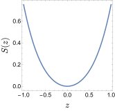
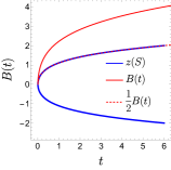
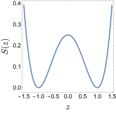
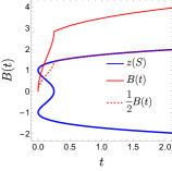
Figure 1: Examples of the correspondence between action and Borel transform. Left shows two quartic actions $S(z)=\frac{1}{2}z^{2}+\frac{1}{4}z^{4}$ and $S(z)=\frac{1}{4}-\frac{1}{2}z^{2}+\frac{1}{4}z^{4}$. Right shows their multivalued inverses $z(S)$ (blue) and Borel transforms (red). The Borel transform is the sum of $|z(S)|$ over different inversion domains.

The higher-dimensional analog of Eq. (9) follows also from Eqs. (6) and (3) and integration in $t$:

$$B(t)=\int d^{n}\vec{z}\ \Theta(t-S(\vec{z}))\,.$$ (10)

Thus $B(t)$ is the volume of the domain for which $S(\vec{z})\leq t$. A physicist might note that $B^{\prime}(t)$ is a kind of density of states, describing the volume of paths or fields with action below a given value. A mathematician might identify $B(t)$ with the sublevel sets for the Morse function $S:M\to{\mathbb{R}}$, where $M$ is the manifold for which $\vec{z}$ are coordinates. Morse theory provides a mapping from critical points of the Morse function to singularities of the Borel transform Pham (1985); Howls (1997); Delabaere and Howls (2002); Witten (2011). Both perspectives are useful.

Borel singularities. Now let us ask: what do singularities in $B(t)$ tell us about $S(\vec{z})$? Eq. (10) shows us that singularities in $B(t)$ can arise in at least three ways: (i) $S(\vec{z})$ has a critical point at some $\vec{z}_{*}$ which leads to a branch point in the Borel plane at $t=S(\vec{z}_{*})$; (ii) $S(\vec{z})$ asymptotes to a constant value $t_{*}$ as one or more of the coordinates $\vec{z}$ go to infinity (e.g. saddles at infinity); (iii) when $t$ hits a certain value $t_{*}$, there is suddenly an infinite coordinate volume for which $S(\vec{z})=t_{*}$, and as such $B(t)$ is divergent for $t>t_{*}$. Instantons in toy 1D models and some QFT instantons like the Fubini instanton in $\phi^{4}$ theory realize (i). Some examples of this class are discussed in App. A. We proceed then to discuss instanton-anti-instanton pairs in QCD, which are only true saddles at infinite separation, realizing (ii). Then we will argue that renormalons realize (iii).

Let us now discuss an example of (ii). Recall that in either QCD or the symmetric double-well potential in QM, there are instanton-anti-instanton pairs (henceforth $\text{I}\hskip 1.00006pt\overline{\text{I}}$) with zero topological charge. Defining $t_{\text{I}}$ be the action of a single instanton, the contribution of $\text{I}\hskip 1.00006pt\overline{\text{I}}$ to the Borel transform of $E_{0}(g)/g$ with $E_{0}(g)$ the ground state energy. In either QCD or QM, the Borel transform has a singularity at $t=2t_{\text{I}}$. Because of Eq. (3), whether this singularity is a pole or logarithmic is unimportant for the present discussion. The key feature is that $B(t)$ diverges at $t=2t_{\text{I}}$. Letting $z$ be the separation between the instanton and anti-instanton, in either QCD or QM the classical action has the form $S(z)=2t_{\text{I}}(1-e^{-z})$ Balitsky and Yung (1986); Babansky and Balitsky (2000). This reflects the fact that $\text{I}\hskip 1.00006pt\overline{\text{I}}$ is only a genuine saddle at infinite separation in the full path integral, and is consistent with Eq. (9) and $B(t)$ blowing up at $t=2t_{\text{I}}$. While the full treatment of such a ‘saddle point at infinity’ in the path integral is subtle, we can demonstrate the essential physics with an initial toy 1D integral

$$f_{\text{I}\hskip 0.70004pt\overline{\text{I}}}(g)=\int_{0}^{\infty}\!\!dz\,e^{-\frac{2t_{\text{I}}}{g}(1-e^{-z})}.$$ (11)

Although this integral is divergent, each term in its perturbative expansion around $g=0$ is finite. The Borel transform of the resulting asymptotic series is $B_{\text{I}\hskip 0.70004pt\overline{\text{I}}}(t)=-\log(1-\frac{t}{2t_{\text{I}}})$, which exhibits the expected singularity at $t=2t_{\text{I}}$.

Now let us more properly take account of Eq. (11) being divergent. Inspecting Eq. (11), we notice that the thimble starting at $z=0$ does not end at $z=\infty$ but continues into the complex plane in one of two ways, characteristic of Stokes phenomena Behtash et al. (2018). Deforming $g\to g\pm i\epsilon$ to break the ambiguity and inserting a cutoff at $z=\Lambda$, we can trace a thimble along three contour segments: $C_{1}=\{0\!<\!z\!<\!\Lambda\}$, $C_{2}^{\pm}=\{z=\Lambda\pm iy\,|\,0\!<\!y\!<\!\pi\}$ and $C_{3}^{\pm}=\{z=\pm i\pi+x\,|\,\Lambda\!>\!x\!>\!-\infty\}$. In the limit $\Lambda\rightarrow\infty$, the sum of the integral along an entire thimble $C^{\pm}=C_{1}\cup C_{2}^{\pm}\cup C_{3}^{\pm}$ is

$$\int_{C^{\pm}}dz~{}e^{-\frac{2t_{\text{I}}}{g}(1-e^{-z})}=-e^{-\frac{2t_{\text{I}}}{g}}E_{1}\!\left(-\frac{2t_{\text{I}}}{g}\pm i\epsilon\right),$$ (12)

which is identical to the lateral inverse Borel transform of $B_{\text{I}\hskip 0.70004pt\overline{\text{I}}}(t)$, as expected. Accordingly, we expect that in full-fledged QCD and QM, the lateral Borel resummation of the leading $\text{I}\hskip 1.00006pt\overline{\text{I}}$ corresponds to a similarly deformed integration contour into complex path or field space.

Finally, we turn to renormalons. Like the $\text{I}\hskip 1.00006pt\overline{\text{I}}$ instanton in QCD, renormalons correspond to singularities in the Borel plane. However, we argue they correspond to mechanism (iii) rather than (ii). Although renormalons require a quantum field theory (to generate the scale anomaly), the mechanism of (iii) can be understood through the lens of an effective action in finite dimensions. Starting from Eq. (4), we can imagine splitting $\vec{z}=(\vec{z}_{1},\vec{z}_{2})$, e.g. $\mathbb{R}^{n}\simeq\mathbb{R}^{n_{1}}\oplus\mathbb{R}^{n_{2}}$, and integrating out $\vec{z}_{2}$. Then we expect to have a residual integral of the form

$$f_{S}(g)\approx\int d^{n_{1}}\vec{z}_{1}\,e^{-\frac{1}{g}\left(S_{0}(\vec{z}_{1})+gS_{1}(\vec{z}_{1})+g^{2}S_{2}(\vec{z}_{1})+\cdots\right)}\,.$$ (13)

For the moment neglecting the terms at higher than one loop order, the analog of Eq. (10) becomes

$$B(t)\approx\int d^{n_{1}}\vec{z_{1}}\ \Theta(t-S_{0}(\vec{z}_{1}))\,e^{-S_{1}(\vec{z}_{1})}\,.$$ (14)

We see that $B(t)$ can diverge for $t$ above some critical $t_{*}$ if $S_{1}(\vec{z}_{1})$ suddenly becomes unstable (e.g. not bounded from below) on the hypersurface $S_{0}(\vec{z}_{1})=t_{*}$. This is an ‘effective action’ manifestation of mechanism (iii).

To be more concrete, consider the provisional toy 2D integral with $S_{0}(s,\rho)=s$ and $S_{1}(s,\rho)=(t_{R}-s)\rho$ :

$$f_{R}(g)=\int_{0}^{\infty}\!ds\int_{0}^{\infty}\!d\rho\,e^{-\frac{1}{g}s-(t_{R}-s)\rho}\,.$$ (15)

This integral is divergent but we will refine it shortly. Notice that $\rho$ appears only in $S_{1}$ and not in $S_{0}$. In the full field theory $\rho$ will correspond to a collective coordinate for (anomalous) scale invariance. Formally we can compute the Borel transform of $f_{R}(g)$ as

$$B_{R}(t)=\int_{0}^{\infty}\!ds\int_{0}^{\infty}\!d\rho\,\Theta(t-s)\,e^{-(t_{R}-s)\rho}\,,$$ (16)

as in Eq. (14). For $t<t_{R}$ the Borel transform is $B_{R}(t)=-\log(1-\frac{t}{t_{R}})$ while if $t\geq t_{R}$ then $B_{R}(t)$ is divergent, since the exponential integral in $\rho$ destabilizes. The action in Eq. (15) has a non-trivial “renormalon” saddle at $(s,\rho)=(t_{R},1/g)$ on the boundary of the instability.

Figure 2: Real part of the action $S_{\text{tot}}=s+g(t_{R}-s)\rho$ shown in orange for $g=t_{R}=1$. This action has a non-trivial ‘renormalon’ saddle at $s=\rho=1$ (blue dot). The planes represent thimbles where the vertical axis is reinterpreted as the direction $w={\text{Im}}~{}s={\text{Im}}~{}\rho$. The steepest ascent surface from the boundary (black lines) is real until it merges with the red plane by the saddle point. This boundary thimble can be deformed into the green half-planes for ease of integration. The renormalon thimble is shown in red.

The divergence of the Borel transform for $t\geq t_{R}$ and of $f_{R}$ in Eq. (15) is similar to the divergence of the $\text{I}\hskip 1.00006pt\overline{\text{I}}$ instanton integral in Eq. (11) and can be corrected in an analagous way: sticking to a thimble. Notice that near the origin $(s,\rho)=(0,0)$, the total action $S_{\text{tot}}=s+g(t_{R}-s)\rho$ grows in the positive $s$ and $\rho$ directions. Near the renormalon the total action grows in one real direction, where ${\text{Re}}\,s=-{\text{Re}}\,\rho$, and one imaginary, where ${\text{Im}}\,s={\text{Im}}\,\rho$. Thus the thimble which begins on the original boundary $\Omega=(s=0,\rho\in{\mathbb{R}}^{+})\cup(s\in{\mathbb{R}}^{+},\rho=0)$ must move into a complex direction to avoid the Stokes point at the saddle. As such, we should really consider a contour in the appropriate relative homology class, such as one which simply moves up from $\Omega$ in the imaginary direction as shown in Fig. 2. Writing $s=x+iw$ and $\rho=y+iw$, this “boundary” thimble is over the $(x,y,w)$ surfaces $C_{1}=({\mathbb{R}}^{+},0,{\mathbb{R}}^{+})$ and $C_{2}=(0,{\mathbb{R}}^{+},{\mathbb{R}}^{+})$, and letting $C=C_{1}\cup C_{2}$ we have the refined integral

$$\int_{C}ds\wedge d\rho\,e^{-\frac{1}{g}S_{\text{tot}}}=-e^{-\frac{t_{R}}{g}}E_{1}\!\left(-\frac{t_{R}}{g}+i\epsilon\right).$$ (17)

Integrating along this 2D thimble which avoids the renormalon Stokes point reproduces the lateral Borel resummation of the $f_{R}(g)$ asymptotic series. The right-hand side has a similar form as that of Eq. (12) for $\text{I}\hskip 1.00006pt\overline{\text{I}}$, but arises by mechanism (iii) rather than mechanism (ii). For completeness, we observe that one can also integrate along a thimble $C_{R}$ passing through the renormalon. In $(x,y,w)$ coordinates this $R$-thimble is the surface where $-\infty<x-t_{R}=1/g-y<\infty$ and $-\infty<w<\infty$. Integrating along this contour gives twice the imaginary part of Eq. (17). We are now ready to examine renormalons in quantum field theory.

Renormalons as saddles. The classic example of a renormalon is the singularity at $t=\frac{2}{\beta_{0}}$ in the Borel transform $B_{A}(t)$ of the Adler function in 4D Yang-Mills coupled to fermions, where $\beta_{0}$ is the leading order $\beta$-function coefficient ’t Hooft (1979); Beneke (1999). This renormalon arises from a chain of vacuum-polarization corrections to the current-current two-point function. More generally, renormalons are believed to occur at $t_{n}=\frac{n}{\beta_{0}}$ for various integers $n$; while this has been shown for QED, it has not been conclusively shown in QCD Beneke (1993). A motivation for this general placement of IR renormalon poles is that the one-loop renormalization group equation (RGE) is solved by $g(\mu)^{-1}=2\beta_{0}\log(\frac{\mu}{\Lambda})$ so that an ambiguity of order $\exp(-t_{n}/g(\mu))=(\frac{\Lambda}{\mu})^{2n}$ can be cancelled by an operator of dimension $2n$ in the OPE. Our goal is next to provide a non-perturbative path integral explanation of the $n=2$ renormalon, ultimately relating it to Eq. (15).

In a classically scale-invariant theory, any nontrivial saddle is degenerate, complicating the method of steepest descent. When scale invariance is broken by quantum effects, the degeneracy is lifted by integrating out UV fluctuations to produce the 1-loop effective action. To see this, consider a classically scale-invariant, relativistic field theory in $D$ Euclidean dimensions. Let the field degrees of freedom be denoted by $\phi(x)$ where we suppress possible indices (e.g. for spin-1 gauge fields) and the classical action by $S_{0}[\phi(x)]$ after the coupling $g$ is scaled out. Our goal is to compute the expectation value of some operator $\mathcal{O}[\phi]$ with scaling dimension $\Delta_{\mathcal{O}}$, namely

$$\langle\mathcal{O}\rangle=\frac{1}{Z}\int[d\phi]\,e^{-\frac{1}{g}S_{0}[\phi]}\mathcal{O}[\phi(x)]\,.$$ (18)

If $\phi$ has classical scaling dimension $\Delta_{\phi}$, then the action is invariant under the simultaneous dilatations and translations $\phi(x)\to R^{-\Delta_{\phi}}\phi(\frac{x-x_{0}}{R})$. It will be prudent to use coordinates on field space which reflect these invariances. In particular, we consider “$R$-coordinates” $(R,x_{0},\Phi(x))$ which parameterize the space of fields as $\phi(x)=\frac{1}{R^{\Delta_{\phi}}}\Phi(\frac{x-x_{0}}{R})$.

A useful basis for $\Phi(x)=\sum_{n=1}^{\infty}a_{n}\Phi_{n}(x)$ is constructed in Andreassen et al. (2018); Bhattacharya et al. (2024) for 4D scalar fields, which generalizes to higher spin fields. We can integrate out the UV modes in the decomposition, corresponding to $\Phi_{n}(x)$ with $n>N$. Defining $\chi(x)\equiv\sum_{n=1}^{N}a_{n}\Phi_{n}(x)$, Eq. (18) becomes

$$\langle\mathcal{O}\rangle=\frac{1}{Z}\int[d\chi]\int\!d^{D}x_{0}\!\int_{R_{0}}^{\infty}\!\!\frac{dR}{R^{D+1}}\,\frac{\mathcal{J}[\chi]}{N_{\text{int}}[\chi]}\,\mathcal{F}_{\mathcal{O}}[\chi]$$ (19)

$$\times\,e^{-\left(\frac{1}{g}-2\beta_{0}\log(\mu R)\right)S_{0}[\chi]+S_{1}[\chi]}\mathcal{O}\big{[}\frac{1}{R^{\Delta_{\phi}}}\chi\big{(}\frac{x-x_{0}}{R}\big{)}\big{]}\,.$$

Above, the dependence on $\log(\mu R)$ is fixed by RG invariance; $S_{1}[\chi]$ is the remainder of the effective action; $\mathcal{F}_{\mathcal{O}}[\chi]$ comes from the contributions of $\mathcal{O}$ after integrating out the UV modes; and ${\mathcal{J}}[\chi]$ and $N_{\text{int}}[\chi]$ are respectively parts of the Jacobian and intersection number Bhattacharya et al. (2024) arising from the transition to $R$-coordinates. The $\beta_{0}\log(\mu R)$ that multiplies the classical action is important and universal Babansky and Balitsky (2000). Depending on the sign of $\beta_{0}$, the above integral may be UV or IR divergent. To isolate the IR renormalon, we have put a lower cutoff $R_{0}$ on the $R$ integral. If the integral is convergent at large $R$ then the IR renormalon is still present, but Borel resummable.

We next integrate over $x_{0}$ and extract the $R$ dependence of the operator $\mathcal{O}$ by dimensional analysis. Changing coordinates to $\rho=\log(\mu R)$, Eq. (19) then becomes

$$\!\int[d\chi]\!\int_{\log(\mu R_{0})}^{\infty}\!\!d\rho\,\mathcal{F}[\chi,\mu]\,e^{-\frac{1}{g}S_{0}[\chi]-\rho(\Delta_{\mathcal{O}}-2\beta_{0}S_{0}[\chi])}\,,$$ (20)

where $\mathcal{F}[\chi,\mu]\equiv\frac{1}{Z}\mu^{\Delta_{\mathcal{O}}}\frac{\mathcal{J}[\chi]}{N_{\text{int}}[\chi]}\mathcal{F}_{\mathcal{O}}[\chi]\,e^{-S_{1}[\chi]}$. The above integral is already quite similar to Eq. (15). Indeed, the effective action in Eq. (20) has saddle points where

$$(1-2\beta_{0}g\rho)\frac{\delta S_{0}}{\delta\chi}=0\,,\qquad S_{0}[\chi]=\frac{\Delta_{\mathcal{O}}}{2\beta_{0}}\,,$$ (21)

which can be solved by $\rho=\frac{1}{2\beta_{0}g}$ or equivalently $R=\frac{1}{\mu}\exp(\frac{1}{2\beta_{0}g})=1/\Lambda$. This is the renormalon. It has the expected classical action and an appropriate scale.

Like Eq. (15), the integral over $\rho$ in Eq. (20) is divergent when the classical action surpasses the renormalon action: $S_{0}[\chi]>\frac{\Delta_{\mathcal{O}}}{2\beta_{0}}$. And, like in Eq. (15) to make a sensible integral one must deform the integration contour onto a thimble (or chain of thimbles). Performing a change of variables in Eq. (20) from $S_{0}[\chi]$ to $s$ and provisionally deforming the $(\rho,s)$ part of the integration contour onto a new contour $C$, we have

$$\int_{C}ds\wedge d\rho\,e^{-\frac{s}{g}-\rho(\Delta_{\mathcal{O}}-2\beta_{0}s)}\widetilde{B}(s)$$ (22)

where

$$\widetilde{B}(s)=\int\limits_{S_{0}[\chi]=s}\![d\sigma(\chi)]\,\frac{\mathcal{F}(\chi,\mu)}{\big{|}\frac{\delta S_{0}[\chi]}{\delta\chi}\big{|}}\,.$$ (23)

Here, $[d\sigma(\chi)]$ is the measure over the level set $S_{0}[\chi]=s$. If $C$ is the boundary thimble, containing the region where where $R=R_{0}$ and $s=\chi=0$, the result will correspond to the lateral Borel resummation of the renormalon asymptotic series, with imaginary part proportional to $i\exp[-\Delta_{\mathcal{O}}/(2\beta_{0}g)]$. If $C$ is the $R$-thimble, which passes through the renormalon, the imaginary part of the integral should also be proportional to the same expression. We note in passing that if the theory has instantons as well as renormalons, these will appear as branch points in $\widetilde{B}(s)$.

For a concrete example of a renormalon in a physical theory, consider the trace of the gluon field strength tensor squared in QCD: ${\mathcal{O}}_{GG}(x)=\alpha_{s}\text{tr}\,[G_{\mu\nu}(x)]^{2}$. This is the leading operator in the OPE for the Adler function. The integral of its expectation value along the $R$ thimble gives

$$\langle{\mathcal{O}}_{GG}(0)\rangle_{R}\approx\frac{i\pi}{\beta_{0}}\,e^{-\frac{2}{\beta_{0}g(\mu)}}\widetilde{B}^{*}=\frac{i\pi}{\beta_{0}}\!\left(\frac{\Lambda}{\mu}\right)^{\!\!4}\widetilde{B}^{*}$$ (24)

where

$$\widetilde{B}^{*}=\frac{1}{2\pi}\int dz\,d\bar{z}\,e^{-z\bar{z}}\widetilde{B}(z)$$ (25)

with $z=s-\frac{2}{\beta_{0}},\bar{z}=\frac{1}{2\beta_{0}g}-\rho$. Eq. (24) is the expected structure of the ambiguity associated with the leading IR renormalon at $t=2/\beta_{0}$ of the Adler function Mueller (1985); Zakharov (1992); Neubert (1995).

Discussion. Identifying renormalons as saddles in the path integral opens up the very exciting possibility of using them to gain insight into the QCD vacuum: do renormalons mediate tunneling? If so, to where? Should the cartoon of the QCD vacuum as infused with instanton gas be supplemented by a renormalon gas? Our work focused on IR renormalons, since they are more phenomenologically important, but similar arguments should hold for UV renormalons. Do these investigations provide any more insight into the applicability of the OPE in QCD? More generally, having a path integral understanding of renormalons as saddles opens a broad new avenue to connect perturbative and non-perturbative physics in quantum field theory.

Acknowledgements. We would like to thank Marco Serone, Semon Rezchikov and Frank Wilczek for valuable conversations. This work was supported in part by the U.S. Department of Energy under contract DE-SC0013607.

Appendix A Borel-Action examples

This appendix gives some examples of how one can reconstruct a 1D action $S(z)$ from the Borel transform $B(t)$ using Eq. (9).

For a first example, consider the stable quartic potential $S_{1}(z)=\frac{1}{2}z^{2}+\frac{1}{4}z^{4}$ as shown in Fig. 1. Then

$$f_{S_{1}}(g)=\int_{-\infty}^{\infty}dz\ e^{-\frac{1}{2g}z^{2}-\frac{1}{4g}z^{4}}=\frac{1}{\sqrt{2}}\,e^{\frac{1}{8g}}\,\mathcal{K}_{\frac{1}{4}}\!\left(\frac{1}{8g}\right)\,.$$ (26)

This function is non-analytic. Its expansion approaching $g=0$ from the positive real direction is asymptotic:

$$f_{1}(g)\sim\sum_{n=0}^{\infty}\sqrt{2g}(-g)^{n}\frac{\Gamma\left(\frac{1}{2}+2n\right)}{n!}\,.$$ (27)

Its Borel transform is

$$B_{1}(t)=\sum_{n=0}^{\infty}\frac{\Gamma(\frac{1}{2}+2n)}{\Gamma\left(n+\frac{3}{2}\right)n!}\sqrt{2t}(-t)^{n}=2\sqrt{\sqrt{1+4t}-1}\,.$$ (28)

This Borel transform has a branch point at $t=-\frac{1}{4}$. It is Borel summable and the inverse Borel transform exactly reproduces $f_{S_{1}}(g)$.

Alternatively, we could compute the Borel transform using Eq. (9). Solving $S(z)=t$ for $z$ gives two real roots $z_{\pm}=\pm\sqrt{\sqrt{1+4t}-1}$. Summing these two roots agrees with Eq. (28), corroborating Eq. (9). Conversely, we can construct the action from the Borel transform by solving Eq. (9) for $S$ and $z$. Expecting at least two domains for a stable action, we set $B(t)=2z$ which leads to $S=t=\frac{z^{2}}{2}+\frac{z^{4}}{4}$ and the original action is reproduced.

Next we consider the unstable quartic, with action $S_{2}(z)=\frac{1}{4}-\frac{1}{2}z^{2}+\frac{1}{4}z^{4}$. Then

$$f_{S_{2}}(g) =\int_{-\infty}^{\infty}dz\ e^{-\frac{1}{g}\left[\frac{1}{4}-\frac{1}{2}z^{2}+\frac{1}{4}z^{4}\right]}$$ (29)

$$=\frac{\pi}{2}\,e^{-\frac{1}{8g}}\left[\mathcal{I}_{-\frac{1}{4}}\!\left(\frac{1}{8g}\right)+\mathcal{I}_{\frac{1}{4}}\!\left(\frac{1}{8g}\right)\right]\,.$$ (30)

For this action, $S_{2}(z)=t$ has two real solutions $z=\pm\sqrt{1+2\sqrt{t}}$ for any positive $t$ and when $0<t<\frac{1}{4}$ two additional real solutions $z=\pm\sqrt{1-2\sqrt{t}}$. The Borel transform is then immediately computed using Eq. (9):

$$B_{2}(t)=\underbrace{-2\sqrt{1-2\sqrt{t}}\ \theta\left(\frac{1}{4}-t\right)}_{\text{domain in the middle}}+\underbrace{2\sqrt{1+2\sqrt{t}}}_{\text{domain on the ends}}\,.$$ (31)

This action and its Borel transform are also shown in Fig. 1 where one can see their relationship graphically.

The unstable quartic has three saddle points at $z=-1,0,1$. Performing the saddle point expansion around each saddle point gives an asymptotic series whose Borel resummation corresponds to the integral along the Lefschetz thimble passing through the saddle. For example, with $z=1+x$, we compute

$$f_{2}^{(1)}(g) =\int_{-\infty}^{\infty}dx\ e^{-\frac{x^{2}}{g}}\sum_{n}\frac{1}{n!}\left(-\frac{x^{3}+\frac{1}{4}x^{4}}{g}\right)^{n}$$ (32)

$$=\sum_{n=0}^{\infty}g^{n+\frac{1}{2}}\frac{\Gamma\left(\frac{1}{2}+2n\right)}{n!}$$ (33)

with Borel transform

$${\mathcal{B}}[f_{2}^{(1)}]=\sum_{n=0}^{\infty}t^{n+\frac{1}{2}}\frac{\Gamma\left(\frac{1}{2}+2n\right)}{n!\,\Gamma\left(\frac{3}{2}+n\right)}=\sqrt{2-2\sqrt{1-4t\pm i\epsilon}}\,.$$ (34)

The branch point at $t=\frac{1}{4}$ corresponds to the action of the Stokes point at $z=0$, which requires a choice of $\pm i$ in the deformation of the thimble contour. The Borel transform of the expansion around the $z=-1$ saddle also gives Eq. (34).

For the $z=0$ saddle, we can pull out the $e^{-S(0)/g}\neq 1$ factor and compute from the series

$${\mathcal{B}}\left[e^{\frac{1}{4g}}f_{2}^{(0)}\right] =\pm i\sum_{n=0}^{\infty}\sqrt{2t}(-t)^{n}\frac{\Gamma\left(\frac{1}{2}+2n\right)}{\Gamma\left(n+\frac{3}{2}\right)n!}$$ (35)

$$=\pm 2i\sqrt{\sqrt{1+4t}-1}\,.$$ (36)

Technically, the expansion of $f_{S_{2}}(g)$ around the $z=0$ saddle is a trans-series where the powers of $g$ are supplemented by $e^{-1/g}$ terms. These can be compensated for by shifting the $t$ integration domain so that

$${\mathcal{B}}[f_{2}^{(0)}](t)=2\sqrt{1-2\sqrt{t}\pm i\epsilon}\,\theta\left(t-\frac{1}{4}\right)\,.$$ (37)

We then check that $2{\mathcal{B}}[f_{2}^{(1)}]+{\mathcal{B}}[f_{2}^{(0)}]$ agrees with Eq. (31). Moreover, we also check that the inverse Borel transform of each separate Borel transform reproduces the integral along the associated Lefschetz thimble.

References

- Lipatov (1977) L. N. Lipatov, Sov. Phys. JETP 45, 216 (1977).
- ’t Hooft (1979) G. ’t Hooft, in The Whys of Subnuclear Physics, edited by A. Zichichi (Springer US, Boston, MA, 1979) pp. 943–982.
- Lautrup (1977) B. E. Lautrup, Phys. Lett. B 69, 109 (1977).
- Gross and Neveu (1974) D. J. Gross and A. Neveu, Phys. Rev. D 10, 3235 (1974).
- Novikov et al. (1984) V. A. Novikov, M. A. Shifman, A. I. Vainshtein, and V. I. Zakharov, Phys. Rept. 116, 103 (1984).
- Beneke and Zakharov (1993) M. Beneke and V. I. Zakharov, Phys. Lett. B 312, 340 (1993).
- Mariño and Reis (2020a) M. Mariño and T. Reis, JHEP 07, 216 (2020a), arXiv:1912.06228 .
- Mariño and Reis (2020b) M. Mariño and T. Reis, JHEP 04, 160 (2020b), arXiv:1909.12134 .
- Schubring et al. (2021) D. Schubring, C.-H. Sheu, and M. Shifman, Phys. Rev. D 104, 085016 (2021), arXiv:2107.11017 .
- Shifman (2015) M. Shifman, Journal of Experimental and Theoretical Physics 120, 386 (2015).
- Shifman (2023) M. Shifman, Phys. Rev. D 107, 045002 (2023), arXiv:2211.05090 .
- Argyres and Unsal (2012a) P. Argyres and M. Unsal, Phys. Rev. Lett. 109, 121601 (2012a), arXiv:1204.1661 .
- Argyres and Unsal (2012b) P. C. Argyres and M. Unsal, JHEP 08, 063 (2012b), arXiv:1206.1890 .
- Dunne and Ünsal (2013) G. V. Dunne and M. Ünsal, Phys. Rev. D 87, 025015 (2013), arXiv:1210.3646 .
- Dunne and Unsal (2012) G. V. Dunne and M. Unsal, JHEP 11, 170 (2012), arXiv:1210.2423 .
- Maiani et al. (1992) L. Maiani, G. Martinelli, and C. T. Sachrajda, Nucl. Phys. B 368, 281 (1992).
- Beneke (1999) M. Beneke, Phys. Rept. 317, 1 (1999), arXiv:hep-ph/9807443 .
- Grozin and Neubert (1997) A. Grozin and M. Neubert, Nuclear Physics B 508, 311 (1997).
- Hoang et al. (2010) A. H. Hoang, A. Jain, I. Scimemi, and I. W. Stewart, Phys. Rev. D 82, 011501 (2010), arXiv:0908.3189 .
- Luke et al. (1995) M. E. Luke, A. V. Manohar, and M. J. Savage, Phys. Rev. D 51, 4924 (1995), arXiv:hep-ph/9407407 .
- Beneke et al. (2017) M. Beneke, P. Marquard, P. Nason, and M. Steinhauser, Phys. Lett. B 775, 63 (2017), arXiv:1605.03609 .
- Hoang et al. (2018) A. H. Hoang, A. Jain, C. Lepenik, V. Mateu, M. Preisser, I. Scimemi, and I. W. Stewart, JHEP 04, 003 (2018), arXiv:1704.01580 .
- Serone et al. (2017) M. Serone, G. Spada, and G. Villadoro, JHEP 05, 056 (2017), arXiv:1702.04148 .
- Tanizaki (2015) Y. Tanizaki, (2015), 10.15083/00073296.
- Cherman et al. (2015) A. Cherman, D. Dorigoni, and M. Unsal, JHEP 10, 056 (2015), arXiv:1403.1277 [hep-th] .
- Dorigoni (2019) D. Dorigoni, Annals of Physics 409, 167914 (2019), arXiv:1411.3585 [hep-th] .
- Pham (1985) F. Pham, Astérisque 130, 11 (1985).
- Howls (1997) C. Howls, Proceedings of the Royal Society of London. Series A: Mathematical, Physical and Engineering Sciences 453, 2271 (1997).
- Delabaere and Howls (2002) E. Delabaere and C. J. Howls, Duke Mathematical Journal 112, 199 (2002).
- Witten (2011) E. Witten, AMS/IP Stud. Adv. Math 50, 347 (2011).
- Balitsky and Yung (1986) I. Balitsky and A. V. Yung, Physics Letters B 168, 113 (1986).
- Babansky and Balitsky (2000) A. Babansky and I. Balitsky, Phys. Rev. Lett. 85, 4211 (2000).
- Behtash et al. (2018) A. Behtash, G. V. Dunne, T. Schaefer, T. Sulejmanpasic, and M. Ünsal, JHEP 06, 068 (2018), arXiv:1803.11533 .
- Beneke (1993) M. Beneke, Nucl. Phys. B 405, 424 (1993).
- Andreassen et al. (2018) A. Andreassen, W. Frost, and M. D. Schwartz, Phys. Rev. D 97, 056006 (2018), arXiv:1707.08124 .
- Bhattacharya et al. (2024) A. Bhattacharya, J. Cotler, A. Dersy, and M. D. Schwartz, (2024), arXiv:2402.18633 .
- Mueller (1985) A. H. Mueller, Nucl. Phys. B 250, 327 (1985).
- Zakharov (1992) V. I. Zakharov, Nucl. Phys. B 385, 452 (1992).
- Neubert (1995) M. Neubert, Phys. Rev. D 51, 5924 (1995), arXiv:hep-ph/9412265 .