Psi-GAN: A power-spectrum-informed generative adversarial network for the emulation of large-scale structure maps across cosmologies and redshifts

Abstract

Simulations of the dark matter distribution throughout the Universe are essential in order to analyse data from cosmological surveys. $N$-body simulations are computationally expensive, and many cheaper alternatives (such as lognormal random fields) fail to reproduce accurate statistics of the smaller, non-linear scales. In this work, we present Psi-GAN (Power-spectrum-informed generative adversarial network), a machine learning model which takes a two-dimensional lognormal dark matter density field and transforms it into a more realistic field. We construct Psi-GAN so that it is continuously conditional, and can therefore generate realistic realisations of the dark matter density field across a range of cosmologies and redshifts in $z\in[0,3]$. We train Psi-GAN as a generative adversarial network on $2\,000$ simulation boxes from the Quijote simulation suite. We use a novel critic architecture that utilises the power spectrum as the basis for discrimination between real and generated samples. Psi-GAN shows agreement with $N$-body simulations over a range of redshifts and cosmologies, consistently outperforming the lognormal approximation on all tests of non-linear structure, such as being able to reproduce both the power spectrum up to wavenumbers of $1~{}h~{}\mathrm{Mpc}^{-1}$, and the bispectra of target $N$-body simulations to within ${\sim}5$ per cent. Our improved ability to model non-linear structure should allow more robust constraints on cosmological parameters when used in techniques such as simulation-based inference.

1 Introduction

The standard model of cosmology, known as $\Lambda$CDM (see e.g. Peebles, 1993), describes a Universe consisting of cold dark matter (CDM), ordinary matter (baryons), and includes the existence of a cosmological constant $\Lambda$ associated with dark energy. $\Lambda$CDM favours that the relative abundance of dark matter is approximately five times that of baryonic matter, making it the predominant form of matter throughout the Universe (Bertone & Hooper, 2018). The model describes a Universe in which galaxies form along and trace the cosmic web structure formed by dark matter, consisting of filaments which connect clusters and surround voids. Although the gravitational effects of dark matter have been observed in many different ways, the nature of dark matter itself remains a mystery (see e.g. Bertone & Tait, 2018, and references therein).

$N$-body simulations are a common tool used to analyse the origin and evolution of the cosmic web structure formed by dark matter (see e.g. Efstathiou et al., 1985; Springel et al., 2005; Springel, 2005; Boylan-Kolchin et al., 2009; Villaescusa-Navarro et al., 2020, 2021; Springel et al., 2021). In its simplest form, running an $N$-body simulation involves initialising a number of massive particles in a cubic box of fixed comoving dimensions, imposing periodic boundary conditions, and then allowing gravity to act on the particles through its gravitational potential (governed by the Poisson equation; Springel et al., 2021). The initial conditions of the $N$-body simulation are often approximated by a Gaussian random density field and, starting from these initial conditions, the positions and velocities of each particle are updated iteratively over a series of timesteps until today ($z=0$).

There exist many different implementations of $N$-body simulations with differing complexity and accuracy. Direct methods, in which the force on each particle with respect to every other particle is calculated for each timestep, are extremely computationally expensive, and so approximations are used to reduce the time taken to run a simulation. These approximations include: tree code methods (Barnes & Hut, 1986), fast-multipole methods (Greengard & Rokhlin, 1987), particle-mesh methods (Hockney & Eastwood, 1988), adaptive mesh refinement (Berger & Oliger, 1984; Bryan et al., 2014), and combinations such as Tree-PM (see e.g. Springel, 2005; Springel et al., 2021). Despite the improvements in speed due to these approximations, $N$-body simulations are still computationally expensive to run and require access to high-performance computing systems. The time and computing resources required to run a sufficient number of $N$-body simulations limits our ability to study the nature of dark matter and the Universe through techniques such as simulation-based inference (Cranmer et al., 2020).

When a significantly large number of simulations is required, it is common to resort to cheaper approximations. One such approximations for describing dark matter fields is to use a lognormal random field (see e.g. Coles & Jones, 1991; Percival et al., 2004; Xavier et al., 2016; Clerkin et al., 2017; Tessore et al., 2023). A lognormal random field can be easily obtained from a given Gaussian random field, and can be entirely described by very few parameters: the mean $\mu$ and variance $\sigma^{2}$ of the associated Gaussian random field, and a shift parameter $\lambda$. A lognormal random field also demonstrates a skew, which is useful in modelling the matter overdensity field given that it varies from values of $-1$ in voids to values in the range of ${\sim}10^{7}$ in clusters. These properties make lognormal random fields a useful approximation of the matter overdensity field. However, as discussed in Xavier et al. (2016) and Tessore et al. (2023), its low computational complexity comes with limitations. Lognormal random fields are able to reproduce a power spectrum to a high level of accuracy as the power spectrum relies only on the amplitudes of Fourier modes. However, they are unable to reproduce accurate statistics that rely on the phases of Fourier modes, which contain much of the information regarding non-linear structure (Coles, 2008).

Recently, machine learning (ML) methods have been used to approximate $N$-body simulations. Rodríguez et al. (2018) and Mustafa et al. (2019) used generative adversarial networks (GANs; Goodfellow et al., 2020) to emulate slices of $N$-body simulations and weak lensing convergence maps, respectively. Perraudin et al. (2019) and Feder et al. (2020) extended this approach from two-dimensional slices to three-dimensional simulation boxes, and showed that GANs are able to reproduce the large-scale and small-scale features of $N$-body simulations. He et al. (2019) and de Oliveira et al. (2020) trained U-Nets (Ronneberger et al., 2015) to learn the non-linear growth of cosmic structure.

More recently, Piras et al. (2023) used a U-Net in a GAN framework to emulate $N$-body simulations by learning how to transform a corresponding lognormal approximation. Shirasaki & Ikeda (2023) similarly used a U-Net in a Cycle GAN (an unpaired image-to-image method; Zhu et al., 2017) framework to learn unpaired translation from lognormal approximations of weak lensing mass maps to non-Gaussian counterparts. Boruah et al. (2024) developed new network layers in order to generate full-sky weak lensing mass maps from lognormal approximations.

While useful, very few methods consider the impact of cosmology and redshift on the structure of the cosmic web. Piras et al. (2023) considered cosmology and redshift dependence for a simplified low-resolution case, however this dependence was not built into the model. Jamieson et al. (2023) encode cosmology dependence into their U-Net-based model to output non-linear displacements and velocities of $N$-body simulation particles based on their linear inputs.

In this paper we aim to improve lognormal approximations through the use of ML techniques, across a range of cosmologies and redshifts. We build upon the work of Piras et al. (2023) by extending their approach to fully capture cosmology and redshift dependence, with the long-term goal of integrating our work into Glass (Tessore et al., 2023). Our approach starts from the Quijote $N$-body simulation suite (Villaescusa-Navarro et al., 2020), which contains $2\,000$ $N$-body simulation boxes with cosmologies sampled from a five-dimensional Latin hypercube. The simulation suite includes snapshots at five redshifts as well as the initial conditions, which we use to create a dataset of pairs of lognormal and $N$-body slices. We train a conditional U-Net in a GAN in order to learn an image-to-image translation between the domains. Our novel method uses the power spectrum of the generated emulation to inform the network during training and guide it towards reproducing the structure of $N$-body simulations across all scales.

Our paper is structured as follows. In Section 2 we describe the data used from the Quijote simulations. In Section 3 we describe the data generation procedure used to obtain a corresponding lognormal slice for each $N$-body simulation slice, our model architecture, as well as our training, validation, and testing methods. In Section 4 we present the results of our method, including evaluating model performance within the domain of the training data, as well as testing its ability to interpolate within the cosmology and redshift spaces. We conclude in Section 5 with a summary of our work, as well as suggestions for future work needed to meet our long-term goal of Glass integration.

2 Data: simulations and matter fields

In this work, we use the Quijote simulation suite (Villaescusa-Navarro et al., 2020). We specifically use simulations from the Latin hypercube, in which the values of the matter density parameter ($\Omega_{\mathrm{m}}$), the baryon density parameter ($\Omega_{\mathrm{b}}$), the Hubble parameter ($h$), the scalar spectral index ($n_{\mathrm{s}}$), and the root mean square of the matter fluctuations in spheres of radius $8~{}h^{-1}~{}\mathrm{Mpc}$ ($\sigma_{8}$) are varied by sampling from a five-dimensional Latin hypercube. We only consider massless neutrinos, and a constant value for the dark energy equation of state parameter $w=-1$ (i.e. a constant $\Lambda$). This Latin hypercube contains $2\,000$ standard simulations, each containing $512^{3}$ dark matter particles in a box with comoving length of $1\,000~{}h^{-1}~{}\mathrm{Mpc}$. The limits of the Latin hypercube are shown in Table 1 along with the corresponding fiducial values. We utilise both the initial conditions at $z=127$ of each simulation, as well as snapshots at redshifts $z\in\{0,0.5,1,2,3\}$, thus forming a dataset spanning a range of cosmologies and redshifts.

Table 1: The limits and fiducial values for each cosmological parameter in the Quijote simulation’s Latin hypercube suite.

Parameter	Limits	Fiducial Value
$\Omega_{\mathrm{m}}$	$\left[0.1,0.5\right]$	$0.3175$
$\Omega_{\mathrm{b}}$	$\left[0.03,0.07\right]$	$0.049$
$h$	$\left[0.5,0.9\right]$	$0.6711$
$n_{\mathrm{s}}$	$\left[0.8,1.2\right]$	$0.9624$
$\sigma_{8}$	$\left[0.6,1.0\right]$	$0.834$

For each simulation, we convert the particles’ positional information to a continuous field through a mass assignment scheme. Throughout this work, we will consider the matter overdensity field $\delta(\mathbf{x})$, defined as:

$$\delta(\mathbf{x})=\frac{\rho(\mathbf{x})}{\bar{\rho}}-1,$$ (1)

where $\rho(\mathbf{x})$ is the matter density at each position $\mathbf{x}$, and $\bar{\rho}$ is the mean density in the simulation box.

We consider a three-dimensional regular grid with $N^{3}=512^{3}$ voxels. The interpolation of the overdensity field over the grid is then obtained by evaluating the continuous function,

$$\tilde{\delta}(\mathbf{x})=\int\frac{\mathrm{d}^{3}\mathbf{x^{\prime}}}{(2\pi)^{3}}W(\mathbf{x}-\mathbf{x^{\prime}})\delta(\mathbf{x^{\prime}}),$$ (2)

where $W(\mathbf{x})$ is the weight function which describes the number of grid points, per dimension, to which each particle is assigned. We utilise the piecewise cubic spline interpolation scheme (Chaniotis & Poulikakos, 2004; Sefusatti et al., 2016) in which the weight function is symmetric, positively defined, and separable such that $W(\mathbf{x})=W_{\mathrm{1D}}(x_{1}/H)W_{\mathrm{1D}}(x_{2}/H)W_{\mathrm{1D}}(x_{3}/H)$, with $H$ being the grid spacing, and $W_{\mathrm{1D}}$ being the unidirectional weight function:

$$W_{\mathrm{1D}}(s)=\begin{cases}\frac{1}{6}(4-6s^{2}+3\lvert s\rvert^{3})&\textrm{if}~{}0\leq\lvert s\rvert<1,\\ \frac{1}{6}(2-\lvert s\rvert)^{3}&\textrm{if}~{}1\leq\lvert s\rvert<2,\\ 0&\textrm{otherwise}.\end{cases}$$ (3)

3 Method

The goal of this work is to be able to train a model that can transform two-dimensional lognormal overdensity fields into more realistic overdensity fields with statistics that match those of the Quijote Latin hypercube across redshifts and cosmologies. In order to do this, we first create a dataset containing pairs of two-dimensional slices of the Quijote Latin hypercube and their corresponding lognormal counterpart (Section 3.1), we then train a machine learning model to apply this transformation (Sections 3.2 and 3.3), and finally validate the model using a set of statistical metrics (Section 3.4).

3.1 Data generation

In order to create the required dataset, we obtain $n=16$ slices for each three-dimensional simulation box by slicing each box along a chosen axis such that each slice has a depth of $32$ pixels. We reduce the dimensions of the slices from three to two by taking the depth-wise mean. The depth of each slice is then given by $1\,000/n~{}h^{-1}~{}\mathrm{Mpc}=62.5~{}h^{-1}~{}\mathrm{Mpc}$, which was chosen to be lower than the approximate depth of matter shells in Glass (von Wietersheim-Kramsta et al., 2024). A shallower depth ensures that more small-scale structure remains in the slices, thus making it more difficult to model. Successfully reproducing slices of this depth, will ensure that Psi-GAN will also be able to reproduce slices of a greater depth. While the matter shells in Glass have varying depth, we leave incorporating this depth dependence into the model to future work. Our training data spans all of the $2\,000$ cosmologies in the Quijote Latin hypercube at redshifts of $z\in\{0,0.5,1,2,3\}$, resulting in $16\times 2\,000\times 5=160\,000$ slices.

In order to generate corresponding lognormal counterpart to each slice we follow the procedure outlined by Piras et al. (2023). While a brief description will be provided here we direct the reader to Piras et al. (2023) for a more detailed description of this procedure.

We start by measuring the two-dimensional power spectrum of each slice $P(k)$. In order to generate a lognormal random field with the given measured power spectrum, we follow Coles & Jones (1991) and Percival et al. (2004). We then convert $P(k)$ to the matter correlation function $\xi_{\mathrm{LN}}(r)$, and calculate the corresponding Gaussian correlation function:

$$\xi_{\mathrm{G}}=\mathrm{ln}\left[1+\xi_{\mathrm{LN}}(r)\right].$$ (4)

We convert this Gaussian correlation function back to Fourier space to obtain a Gaussian power spectrum $P_{\mathrm{G}}(k)$.

A zero-mean Gaussian field is entirely defined by its power spectrum which depends only on the absolute values of the Fourier coefficients, therefore the Fourier phases can be uniformly sampled in the interval $[0,2\pi)$ in order to create a realisation of a Gaussian random field (Chiang & Coles, 2000; Coles & Chiang, 2000; Watts et al., 2003). However, as we aim to generate Gaussian random fields $\delta_{\mathrm{G}}$ with high correlations to each given $N$-body slice, we instead use the set of phases from the corresponding slice of the initial conditions at $z=127$. The lognormal field $\delta_{\mathrm{LN}}$ is then calculated by evaluating

$$\delta_{\mathrm{LN}}=\mathrm{exp}\left(\delta_{\mathrm{G}}-\sigma_{\mathrm{G}}^{2}/2\right)$$ (5)

for each grid point, where $\sigma_{G}$ is the standard deviation of the Gaussian field. For these operations, we used the Python package nbodykit (Hand et al., 2018).

There are two limitations to this method due to the fact that we are measuring the power spectrum from a grid. Firstly, due to relying only on the simulation boxes for the measured power spectrum, we are only able to survey a limited range of $k\in[0.025,1]~{}h~{}\mathrm{Mpc}^{-1}$. In order to access larger scales, we use Class (Blas et al., 2011) to generate a theoretical power spectrum for $k\in[10^{-5},0.025]~{}h~{}\mathrm{Mpc}^{-1}$ and concatenate this with the measured power spectrum.

Secondly, we observe a discrepancy in the power spectrum of the generated lognormal field and the measured power spectrum from the Quijote slice. This can be attributed to correlations in phases being introduced when converting the Quijote initial conditions (obtained by second-order Lagrangian perturbation theory) to a density field. We correct for this discrepancy by iteratively re-scaling the Gaussian power spectrum by the ratio of the power spectrum of the lognormal field output and the measured power spectrum of the target slice at each $k$. We iterate through this process until the discrepancy is less than $0.1$ per cent at all $k$ values.

We are left with a dataset of pairs of lognormal and Quijote slices ($\delta_{\mathrm{LN}}$ and $\delta_{\mathrm{NB}}$), which we split into a number of sets. We firstly reserve all slices across all redshifts of cosmologies $\#1586$ and $\#815$ (randomly selected) as part of the test set in order to test model performance on unseen cosmologies. As we only have snapshots at certain redshifts, we create an additional set of lognormal slices at redshift $z\in\{0.25,0.75\}$ for cosmology $\#663$ (which we will refer to as our “fiducial” cosmology from now on, as it is the closest cosmology in our dataset to the Quijote fiducial cosmology) in order to test the model’s ability to interpolate between redshifts. We follow the previously outlined procedure for producing these lognormal slices. However as we have no Quijote snapshots at these redshifts (and are therefore unable to measure a power spectrum), we create a “measured” power spectrum by linearly interpolating the power spectrum at each value of $k$ between redshift snapshots. Furthermore, we reserve $512$ randomly chosen slices at each redshift as part of a test set to assess model performance on cosmologies and redshifts within the training set. $10$ per cent of the remaining dataset is used for validation, with the other 90 per cent being used for training. Table 2 summaries these six sets of data used in the training, validating, and testing of our model.

Table 2: A summary of the datasets used in training (bottom division), validating (middle division), and testing (top division) our model.

Set name	Description	Cosmology	Redshift
Interpolate cosmology test set $\#1$	Testing on reserved cosmology, unseen during training process	Simulation $\#1586$	$z\in\{0,0.5,1,2,3\}$
Interpolate cosmology test set $\#2$	Testing on reserved cosmology, unseen during training process	Simulation $\#815$	$z\in\{0,0.5,1,2,3\}$
Interpolate redshift test set	Testing interpolation between redshifts	Simulation $\#663$	$z\in\{0.25,0.75\}$
Randomly split test set	Testing within the domain of the training data using randomly chosen slices at each $z$	Randomly selected from all simulations (excluding $\#1586$ and $\#815$)	$z\in\{0,0.5,1,2,3\}$
Validation set	Validating the model using 10 per cent of the remaining slices not used for testing	All simulations (excluding $\#1586$ and $\#815$)	$z\in\{0,0.5,1,2,3\}$
Training set	Training the mode with 90 per cent of the remaining slices not used for testing	All simulations (excluding $\#1586$ and $\#815$)	$z\in\{0,0.5,1,2,3\}$

3.2 Model architecture

We train a Wasserstein GAN with gradient penalty (WGAN-GP; Arjovsky et al., 2017; Gulrajani et al., 2017) consisting of a generator and a critic. In a traditional GAN, the generator and critic are adversarially trained in tandem in order to produce generated data that is identical to real data. Our approach builds physics into the critic of the GAN to constrain the generator to produce data that is physically consistent with the target domain. A full schematic of the Psi-GAN framework can be found in Figure 1. In this figure, we demonstrate how an emulation can be generated by feeding a lognormal density field, along with its associated cosmology and redshift, into the generator. This framework is trained via a loss function which depends on the output of our physics-informed critic, which takes as inputs either an emulated or $N$-body map, its associated power spectrum, its associated cosmology and redshift, and finally the power spectrum of the corresponding lognormal density field.

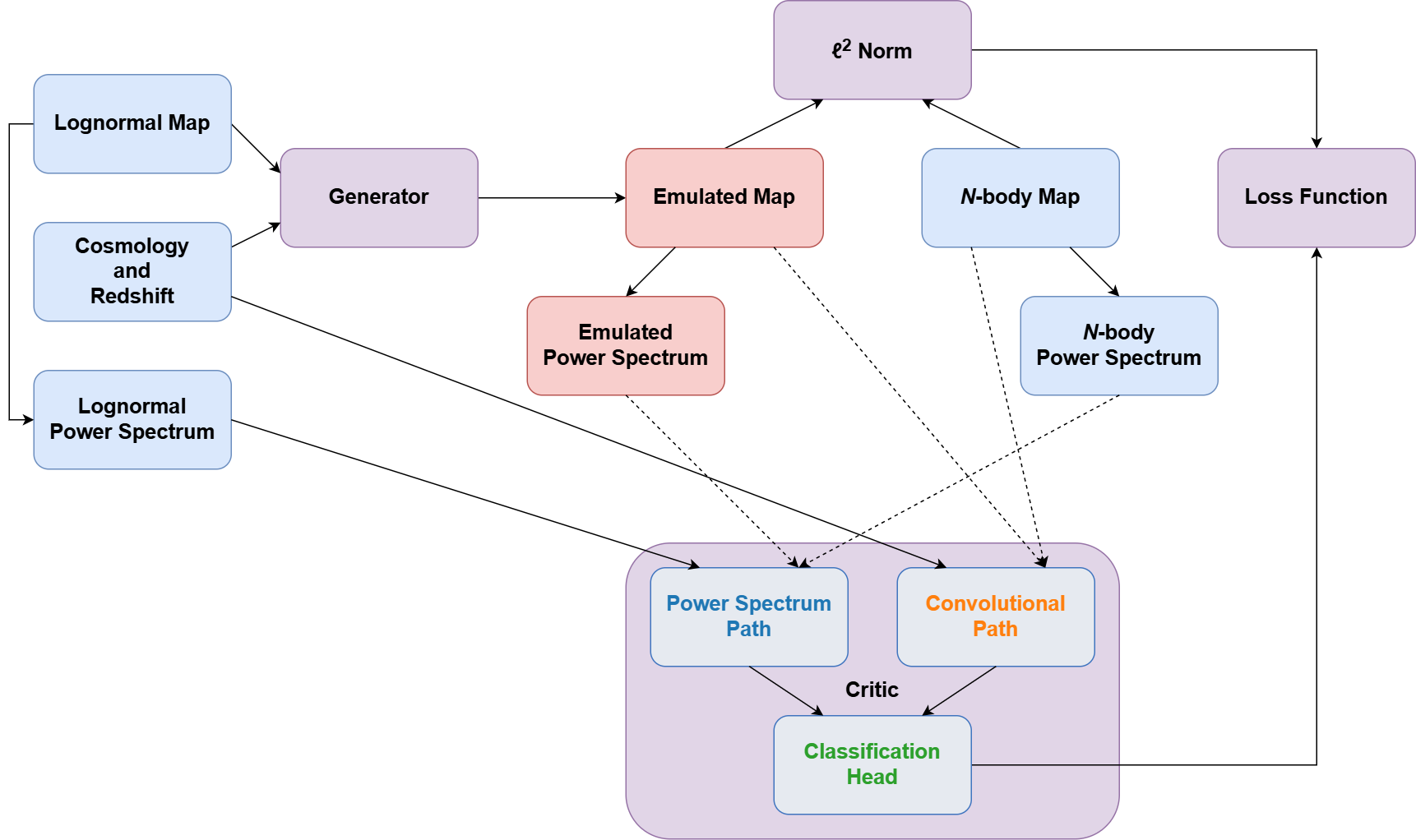
Figure 1: A schematic showing the full construction of the Psi-GAN framework. Data which are part of the initial dataset are coloured in blue, while data that are calculated by the Psi-GAN framework are coloured in red. All computational steps are coloured in purple. Note that the critic takes in either an emulated map or an $N$-body map as an input (along with their associated power spectrum), which is indicated by dashed lines. The internal structure of the critic is also shown, and can be seen in more detail in Figure 2.

Details regarding the computation blocks used to construct Psi-GAN along with the construction of the generator itself can be found in Appendix A, while the construction of the critic is shown in Figure 2. The critic consists of two paths, a convolutional path and a power spectrum path (shown in orange and blue, respectively). The convolutional path takes an input image (with cosmology and redshift embeddings) and processes it using a pre-trained ResNet-50 model (He et al., 2016) to obtain a feature representation of the input. The power spectrum path takes the power spectrum of the input image and compares this to the power spectrum of the corresponding lognormal map via an elementwise subtraction. Both the feature representation and the power spectrum comparison are concatenated and then fed into a linear classifier, along with another set of cosmology and redshift embeddings.

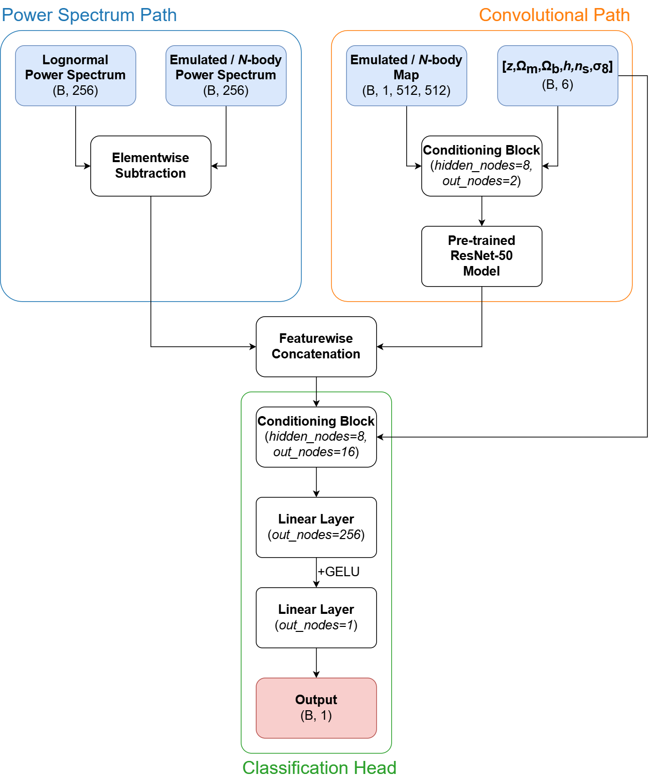
Figure 2: A schematic showing the construction of our critic. The power spectrum path, convolutional path, and classification head are outlined and labelled in blue, orange, and green, respectively. We also provide information, in parentheses, regarding the dimensions for both the inputs (blue) and outputs (red) in roman font, and the hyperparameters of each layer in italics. Dimensions are quoted in the “batch, channels, $\ast$” convention, where $\ast$ represents any number of latent dimensions and B is used as a placeholder for the batch dimension of all inputs and outputs. All convolutional layers use circular padding in order to maintain the height and width of the input, and GELU represents the Gaussian Error Linear Unit (Hendrycks & Gimpel, 2016). The conditioning block is used to inform the network of the cosmology and redshift of the emulation, and is defined in Appendix A.

GANs for image synthesis often use a purely feature-based network for the critic, however using a fully-convolutional critic resulted in the generator altering the power spectrum of its input when attempting to generate a more realistic output. The power spectrum path was then added to the critic in order to guide the generator towards not altering the power spectrum. As the lognormal input to the generator has a matching power spectrum to their corresponding $N$-body slices, any deviation away from this would be indicative of a generated map, and therefore this information is extremely helpful for the critic to be able to differentiate between a real and generated image. This information is also able to be backpropagated through the critic and generator networks to ensure that the generator is trained to capture features at all scales.

Both the generator and the critic are trained in tandem in order to minimise the loss function $L_{\mathrm{train}}$, which we choose to be the standard WGAN-GP formulation with an additional term equating to the $l^{2}$ norm between out generated map and the target $N$-body slice:

$$L_{\mathrm{train}}=L_{\mathrm{G}}+L_{\mathrm{NB}}+L_{\mathrm{GP}}+L_{\mathrm{pixel}},$$ (6)

where each component of the training loss is given by:

$$L_{\mathrm{G}}=\mathbb{E}_{G(\delta_{\mathrm{LN}})}[C(G(\delta_{\mathrm{LN}}))],$$ (7)

$$L_{\mathrm{NB}}=-\mathbb{E}_{\delta_{\mathrm{NB}}}[C(\delta_{\mathrm{NB}})],$$ (8)

$$L_{\mathrm{GP}}=\lambda_{\mathrm{gp}}\mathbb{E}_{\hat{\delta}}\left[\left(\lvert\lvert\nabla_{\hat{\delta}}C(\hat{\delta})\rvert\rvert_{2}-1\right)^{2}\right],$$ (9)

$$L_{\mathrm{pixel}}=\lambda_{\mathrm{pixel}}\lvert\lvert G(\delta_{\mathrm{LN}})-\delta_{\mathrm{NB}}\rvert\rvert^{2}_{2},$$ (10)

where $G$ and $C$ are the generator and critic networks respectively, $\delta_{\mathrm{LN}}$ and $\delta_{\mathrm{NB}}$ are lognormal and $N$-body simulation slices, $\hat{\delta}$ represents a linear combination of $G(\delta_{\mathrm{LN}})$ and $\delta_{\mathrm{NB}}$, $\mathbb{E}$ represents the expectation over a sample, $\lvert\lvert\cdot\rvert\rvert_{2}$ represents the $l^{2}$ norm, and $\lambda_{\mathrm{gp}}$ and $\lambda_{\mathrm{pixel}}$ are hyperparameters used to control the amount of regularisation from the gradient penalty and $l^{2}$ norm between the generated output and the target. We set $\lambda_{\mathrm{gp}}=10$ and $\lambda_{\mathrm{pixel}}=100$, however we leave the optimisation of these hyperparameters to future work.

3.3 Training

We train using the Adam optimiser (Kingma & Ba, 2014) with a base learning rate $\alpha=10^{-4}$, and decay parameters $\beta_{1},\beta_{2}=0.5,0.9$. Following Heusel et al. (2017), we increase the learning rate for the critic by a factor of $f=3$ while using the base rate for the generator. We allow the model to train for an initial period of three epochs, after which we half the learning rate after every epoch where the validation loss increases. We also employ gradient clipping to clamp the magnitude of the gradients to a maximum value of $1\,000$. The gradient penalty term in the loss function should act to keep gradients close to unity, however there is a warm up period until it is able to have its intended effect. Clipping the gradients was found to be useful in avoiding overflow errors before the gradient penalty took effect.

We train using a batch size of $6$, and use randomised data augmentation techniques when compiling a batch. The same data augmentations were applied both $\delta_{\mathrm{LN}}$ and $\delta_{\mathrm{NB}}$ and consist of:

1. horizontal and vertical flips,

2. horizontal and vertical translations of $x,y\in[0,512)$ pixels,

3. rotations of $\theta\in\left\{0,\pi/2,\pi,3\pi/2\right\}$.

We use $32$-bit floating point precision for numerical stability. A single epoch of training and validation takes ${\sim}15$ hours on a single NVIDIA A100 Tensor Core GPU, and we train for $10$ epochs. Training time is significantly inflated as the critic requires the power spectrum to be calculated for each generated sample in the dataset. However, we accelerate this computation by using a parallelised GPU implementation. We also pre-compute power spectra for all $\delta_{\mathrm{LN}}$ and $\delta_{\mathrm{NB}}$ in our dataset so that they do not need to be calculated during training. Once trained, the generator can process $512$ lognormal slices in ${\sim}2$ minutes on similar hardware.

3.4 Validation and testing

We validate and test our model using a range of summary statistics which will be described in this section. We save the model after each training epoch, and select the best model using a weighted sum of the absolute percentage error across the summary statistics (excluding the bispectrum and reduced matter bispectrum, due to the complexity of their calculation). We weight the summary statistics such that the power spectrum has a weighting seven times that of the other statistics in order to bias our model selection towards a model that reproduces an accurate power spectrum. We also add redshift-dependent weighting to the validation loss, with redshift $z=0$ examples being given double the weighting of all other redshifts. This is to bias model selection towards a model that performs well at low redshifts. To test the model, we quantitatively compare these summary statistics for the lognormal slices, generated slices, and $N$-body slices in each of the test sets described in Table 2.

3.4.1 Pixel counts histogram

We bin the pixel values of the lognormal, generated, and $N$-body slices into a histogram of $64$ equally sized bins. The ranges that these bins span differ depending on redshift, and were qualitatively chosen in order to ensure that all bins have a count of at least $10$ pixels in order to avoid divide-by-zero errors when computing relative differences. It can be seen in Section 4 that the lognormal approximation differs significantly from the target $N$-body distribution, while our model aims to improve over the lognormal.

3.4.2 Peak counts histogram

We use peak counts to assess whether the model has learned the non-Gaussian features of the $N$-body field. A peak is defined as a pixel with a higher value than all of its eight surrounding pixels. We bin peak count values into a histogram of $64$ equally sized bins in order to compare non-Gaussian information between different models. Similarly to the pixel counts histogram, the ranges of these bins differ by redshift and were chosen in order to avoid divide-by-zero errors when calculating errors. Peak count statistics have been shown to carry significant cosmological information, especially in cosmic shear studies (Pires et al., 2012; Lin & Kilbinger, 2015a, b; Lin et al., 2016; Kacprzak et al., 2016; Shan et al., 2018; Martinet et al., 2018; Harnois-Déraps et al., 2021; Zürcher et al., 2022; Harnois-Deraps et al., 2024).

3.4.3 Phase difference distribution

The phases of Fourier modes are an important measure of non-linearity in the cosmic web. While a Gaussian field exhibits randomised phases, non-linear structure growth introduces correlations into the phases. While the power spectrum relies only on Fourier amplitudes, it has been shown that the phases carry substantial information regarding the structure of the matter overdensity field (Coles, 2008) thus making phase statistics extremely important in analysing the cosmic web.

Many methods exist to quantify phase statistics, including calculating the entropy of Fourier phases and measuring the distribution of phases (see e.g. Chiang & Coles, 2000; Coles & Chiang, 2000; Watts et al., 2003; Matsubara, 2003, 2007). We focus on the probability distribution of phase differences as described by Watts et al. (2003), in which the authors define a quantity $D_{k}$ given by:

$$D_{k}=\Phi_{k+1}-\Phi_{k},$$ (11)

which measures the difference in the phases of adjacent Fourier modes (in a single dimension) $k$ and $k+1$. This can be extended to a two-dimensional field by calculating a set of $D_{k}$ in two orthogonal directions. Watts et al. (2003) find that the distribution of these phase differences $P(D)$ can be described by a von Mises distribution:

$$P(D)=\frac{1}{2\pi I_{0}(\kappa)}e^{-\kappa\mathrm{cos}(D-\mu)},$$ (12)

where $\mu$ is the mean angle which varies from sample to sample, $\kappa$ is a parameter that describes the level of non-linearity, and $I_{0}$ is a modified Bessel function of order zero.

In order to measure $P(D)$ for a dark matter overdensity map, we bin the phase differences into histograms of $64$ equally spaced bins which we use to assess whether the model has correctly learned non-linear growth through phase statistics.

3.4.4 Power spectrum

Although the lognormal input to the model and the target $N$-body simulation have the same power spectrum, we cannot ensure that our model does not significantly alter it. In order to assess whether the power spectrum has been significantly changed, we use the estimator

$$\hat{P}(k)=\frac{1}{N_{\mathrm{modes}}(k)}\sum_{\lvert\mathbf{k}\rvert=k}\lvert\delta(\mathbf{k})\rvert^{2},$$ (13)

where $\delta(\mathbf{k})$ is the Fourier transform of the matter overdensity $\delta(\mathbf{x})$, the summation is performed over all $\mathbf{k}$ vectors with a magnitude of $k$, and $N_{\mathrm{modes}}(k)$ is the number of modes in each $k$ bin.

3.4.5 Bispectrum

Since the power spectrum is unable to capture any information regarding Fourier phases, we can use the matter bispectrum $B(k_{1},k_{2},k_{3})$ to quantify non-linear structure. The bispectrum can be seen as a three-point counterpart to the power spectrum (Sefusatti et al., 2006). The bispectrum for a two-dimensional field is defined by the relation:

$$\langle\delta(\mathbf{k}_{1})\delta(\mathbf{k}_{2})\delta(\mathbf{k}_{3})\rangle=(2\pi)^{2}\delta_{\mathrm{D}}(\mathbf{k}_{1}+\mathbf{k}_{2}+\mathbf{k}_{3})B(k_{1},k_{2},k_{3}),$$ (14)

where $k_{i}=\lvert\mathbf{k}_{i}\rvert$, all $\mathbf{k}_{i}$ vectors are in the plane of the two-dimensional slice, $\delta_{\mathrm{D}}(\cdot)$ indicates the Dirac delta function, and $\langle\cdot\rangle$ represents an expectation value over all Fourier space.

We also assess the reduced matter bispectrum $Q(k_{1},k_{2},k_{3})$ (see e.g. Scoccimarro, 2000):

$$Q(k_{1},k_{2},k_{3})=\frac{B(k_{1},k_{2},k_{3})}{P(k_{1})P(k_{2})+P(k_{1})P(k_{3})+P(k_{2})P(k_{3})}.$$ (15)

We measure the bispectra and reduced matter bispectra based on an estimator of the binned bispectrum (Coulton et al., 2019; Coulton & Spergel, 2019). We report the measurements as a function of the angle $\theta$ between the vectors $\mathbf{k}_{1}$ and $\mathbf{k}_{2}$ using two different configurations: $(k_{1},k_{2})=(0.4,0.4)~{}h~{}\mathrm{Mpc}^{-1}$ and $(k_{1},k_{2})=(0.4,0.6)~{}h~{}\mathrm{Mpc}^{-1}$. Bispectra can be measured along different triangle configurations, and it is important to use many configurations when using the bispectrum as a statistical tool in order to break degeneracies when inferring cosmological parameters (Berge et al., 2010). Therefore we measure the bispectra and reduced bispectra using two configurations: $(k_{1},k_{2})=(0.4,0.6)~{}h~{}\mathrm{Mpc}^{-1}$ and $(k_{1},k_{2})=(0.4,0.4)~{}h~{}\mathrm{Mpc}^{-1}$.

4 Results

Visual inspection shows that Psi-GAN is able to accurately reproduce the structure of the cosmic web across all redshift bins. Figure 3 shows a set of examples for simulation $\#663$, our “fiducial” cosmology.

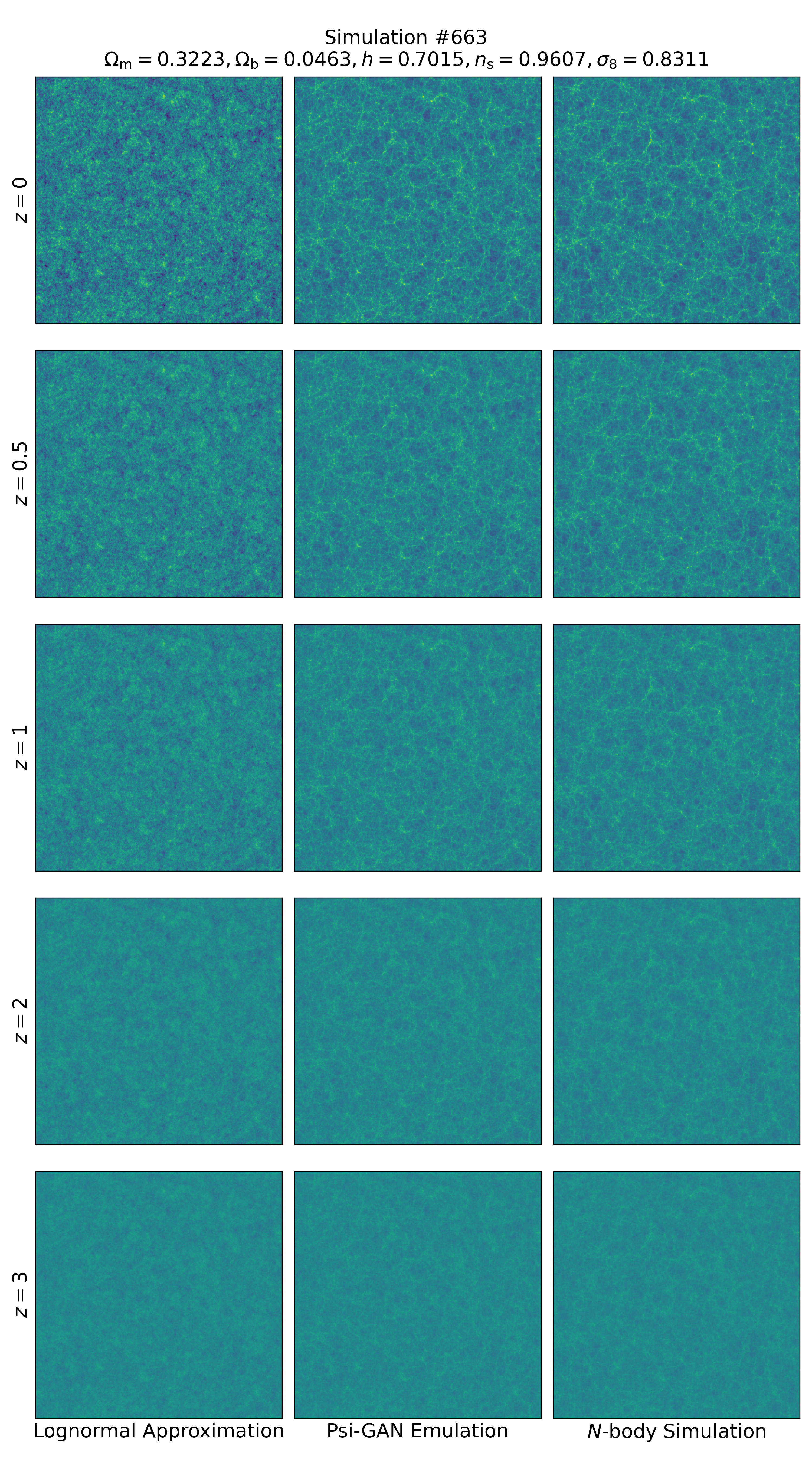
Figure 3: A set of examples for our “fiducial” cosmology, showing lognormal random fields (left), Psi-GAN generated emulations (centre), and $N$-body simulations (right) for all redshift bins.

In addition, Figure 4 shows example maps at redshift $z=0$ for our “fiducial” cosmology, as well as extreme values of the $\Omega_{\mathrm{m}},\sigma_{8}$ subspace. Table 3 shows the values for the chosen cosmologies.

Table 3: The cosmologies used to demonstrate Psi-GAN’s emulations in Figure 4.

Cosmology	$\Omega_{\mathrm{m}}$	$\Omega_{\mathrm{b}}$	$h$	$n_{\mathrm{s}}$	$\sigma_{8}$
“Fiducial”	$0.3223$	$0.04630$	$0.7015$	$0.9607$	$0.8311$
Low $\Omega_{\mathrm{m}}$, Low $\sigma_{8}$	$0.1663$	$0.04783$	$0.6173$	$1.1467$	$0.6461$
Low $\Omega_{\mathrm{m}}$, High $\sigma_{8}$	$0.1289$	$0.06325$	$0.7293$	$1.1537$	$0.9489$
High $\Omega_{\mathrm{m}}$, Low $\sigma_{8}$	$0.4599$	$0.04055$	$0.7287$	$0.8505$	$0.7011$
High $\Omega_{\mathrm{m}}$, High $\sigma_{8}$	$0.4423$	$0.03533$	$0.8267$	$1.0009$	$0.9151$

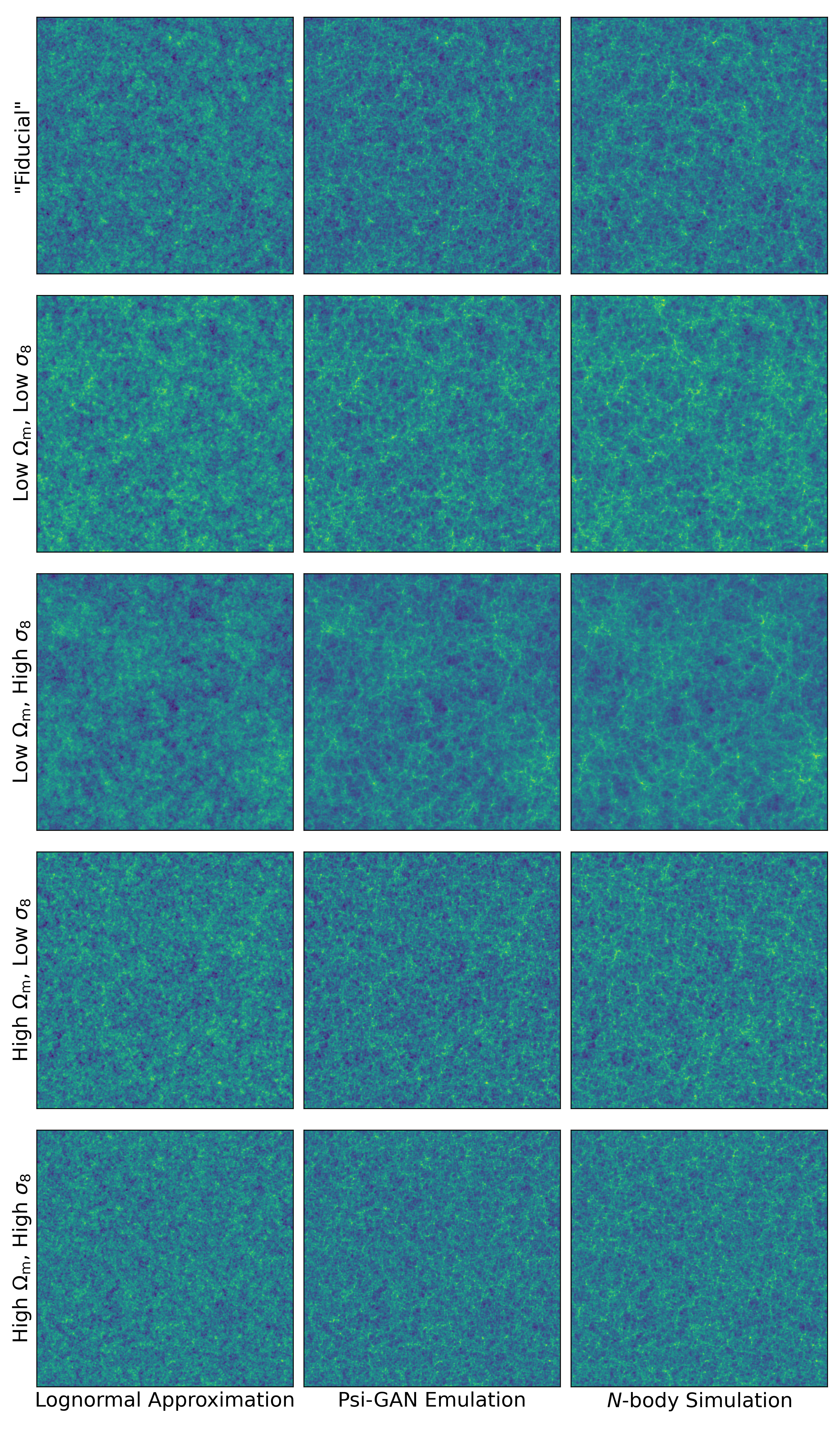
Figure 4: A set of examples for our “fiducial” cosmology and extreme values of the $\Omega_{\mathrm{m}},\sigma_{8}$ subspace (as defined in Table 3), showing lognormal random fields (left), Psi-GAN generated emulations (centre), and $N$-body simulations (right) for redshift $z=0$.

4.1 Randomised test set

Figure 5 shows the results of all eight test metrics for our randomised test set for redshift $z=0$. On the top panel for each metric we show the mean value averaged over $64$ examples of the $N$-body simulation, the Psi-GAN emulation, and the lognormal approximation. On the bottom panel we show the relative difference with respect to the $N$-body simulation for each model. We include uncertainties only on the bottom panel for the sake of visual clarity.

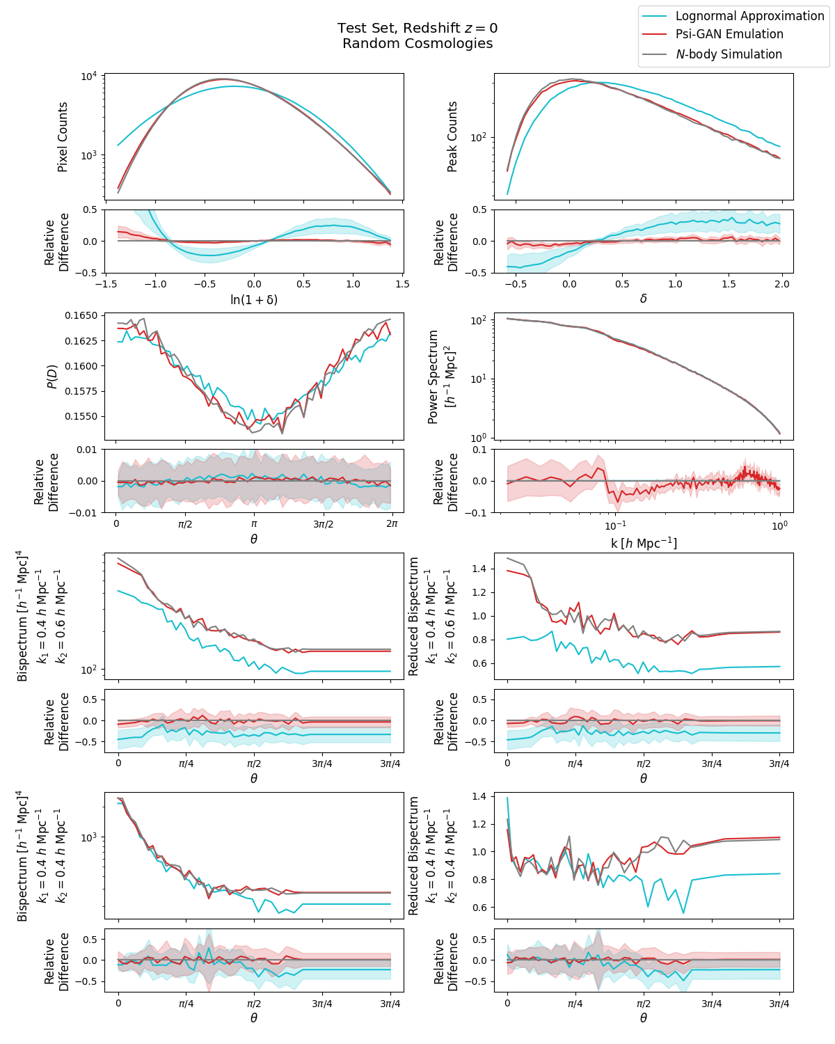
Figure 5: A comparison of the statistical tests as described in Section 3.4 for the lognormal approximation (cyan), $N$-body simulation (grey), and Psi-GAN emulation (red) on the randomised test set. The metrics displayed are as follows (from top to bottom, and left to right): pixel counts, peak counts, phase difference distribution, power spectrum, bispectrum with $(k_{1},k_{2})=(0.4,0.6)~{}h~{}\mathrm{Mpc}^{-1}$, reduced bispectrum with $(k_{1},k_{2})=(0.4,0.6)~{}h~{}\mathrm{Mpc}^{-1}$, bispectrum with $(k_{1},k_{2})=(0.4,0.4)~{}h~{}\mathrm{Mpc}^{-1}$, and reduced bispectrum with $(k_{1},k_{2})=(0.4,0.4)~{}h~{}\mathrm{Mpc}^{-1}$. The relative performance with respect to the $N$-body simulation can be seen in in the bottom panel for each test, along with the respective uncertainties. We show that Psi-GAN outperforms the lognormal approximation across all tests with the exception of the power spectrum, in which we see small discrepancies within $5$ per cent.

In addition, in Figure 6, we show the relative differences averaged over $64$ examples for each model, for all redshifts when compared to $N$-body simulations. We also display the relative differences for the lognormal approximation for comparison. We show all redshift snapshots on the top two panels, however we only show redshift $z=0$ on the remaining panels for visual clarity.

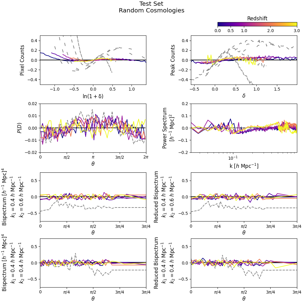
Figure 6: A comparison of the relative differences in the statistical tests as described in Section 3.4 for the lognormal approximation (grey dashed line with looser dash spacing indicating a lower redshift snapshot), $N$-body simulation (black line), and Psi-GAN emulation (lines coloured with respect to the redshift colour at the top of the figure) on the randomised test set. The metrics shown are the same as in Figure 5. We show that Psi-GAN outperforms the lognormal approximation across all tests with the exception of the power spectrum, in which we see small discrepancies within $5$ per cent. Uncertainties are similar to those shown in Figure 5, but are omitted here for visual clarity.

Psi-GAN shows an improvement over the lognormal approximation with the sole exception of the power spectrum. The lognormal approximation was designed to have an identical power spectrum to the $N$-body simulation, so this was an expected result. However, we can say that the power spectrum path in the critic of Psi-GAN was effective in constraining the power spectrum so that it was not altered by more than ${\sim}5$ per cent. Initial trials of an GAN using a fully convolutional critic (i.e. without the power spectrum path) saw differences in the power spectrum between the emulation and the $N$-body simulation of ${\sim}20$ per cent. Thus we can be confident that our critic architecture is effective in maintaining the power when transforming a lognormal random field.

We see agreement to within ${\sim}5$ per cent for all metrics, with the exception of the pixel counts at low values of $\mathrm{ln}(1+\delta)$. This is due to the baseline count for the $N$-body simulation being very low (${\sim}10^{2}$), and thus making the relative differences sensitive to small changes in pixel counts.

4.2 Redshift interpolation

Figure 7 displays similar results to Figure 5, but for our redshift interpolation test at $z=0.25$. On the bottom panel we show the relative difference with respect to a value interpolated between the two adjacent redshift snapshots ($z=0$ and $z=0.5$) as we have no $N$-body snapshot to act as the ground truth.

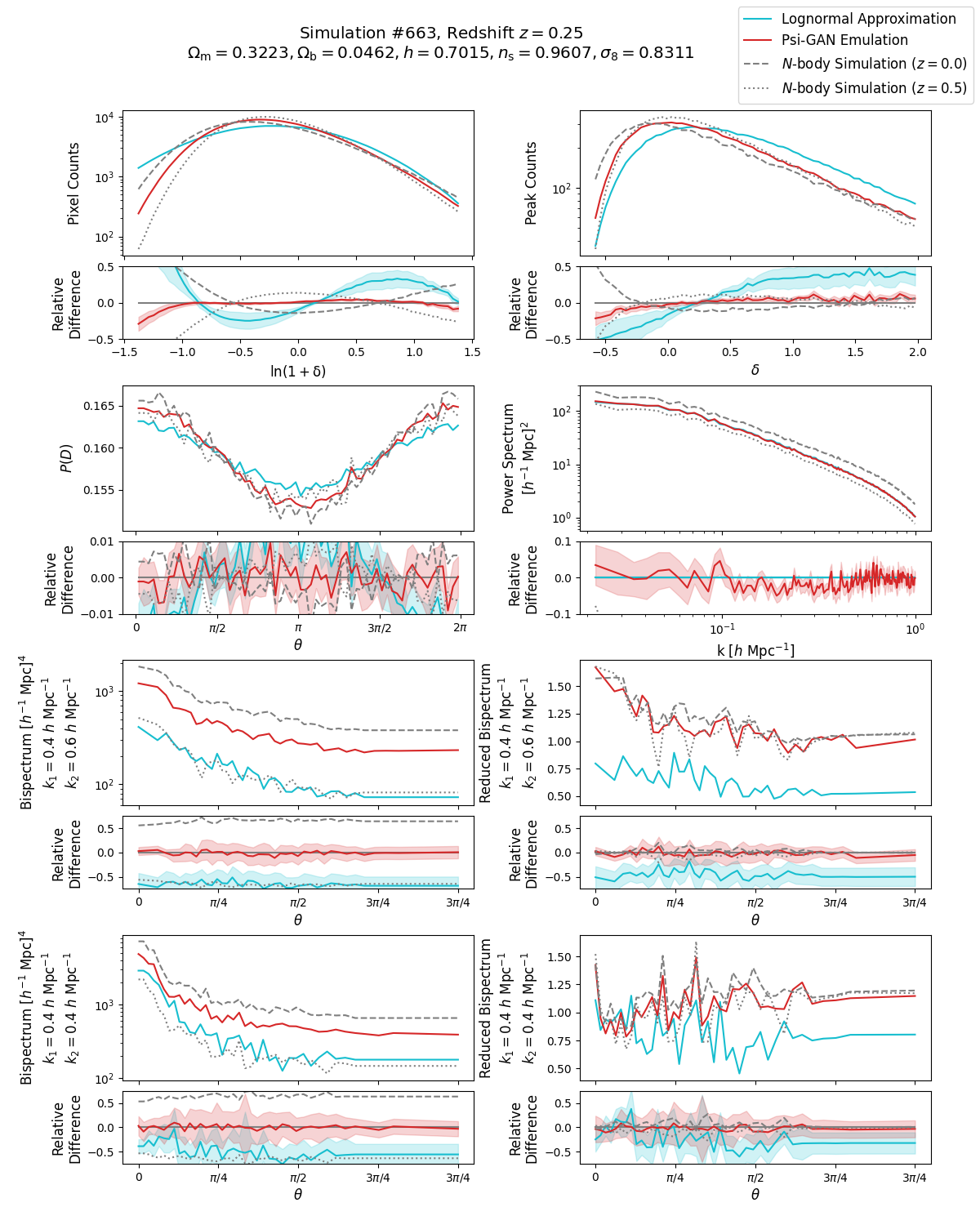
Figure 7: Similar to Figure 5, but for the test set for interpolating redshift at $z=0.25$. As we have no $N$-body snapshot to act as the ground truth, relative differences are displayed with respect to a value interpolated between the two adjacent redshift snapshots. The dashed grey lines show the measured values for these snapshots. Also, please note that the grey dashed lines line outside of the range of the y-axis for the relative differences plot of the power spectrum.

It can be seen that Psi-GAN improves on the lognormal approximation across all metrics. Although not much can be quantitatively said about the performance of Psi-GAN with respect to the $N$-body snapshots, we can qualitatively say that the results lie reasonably between the upper and lower bounds set by the adjacent redshift snapshots (as shown in Figure 7), and within ${\sim}5$ per cent of an interpolated baseline. We can also see that Psi-GAN’s metrics intercept the $N$-body snapshots exactly at cross-over points for the pixel counts, peak counts, and phase difference distributions. We can also see that the power spectrum does not vary by more than $3$ per cent from the lognormal approximation at redshift $z=0.25$, again showing the effectiveness of the power spectrum path in Psi-GAN’s critic.

Our second redshift interpolation test at redshift $z=0.75$ showed similar results to the test at $z=0.25$, but are not shown here for brevity. All metrics showed agreement with $N$-body simulations to within ${\sim}5$ per cent, with the power spectrum showing closer agreement to ${\sim}3$ per cent. The only case of the agreement differing by more than this when the pixel and peak counts histograms were at a very low baseline value (${\sim}10^{2}$), where we saw discrepancies of ${\sim}15$ per cent.

4.3 Cosmology interpolation

Figure 8 displays similar results to Figure 5, but for our cosmology interpolation test for simulation $\#1586$ at redshift $z=0$.

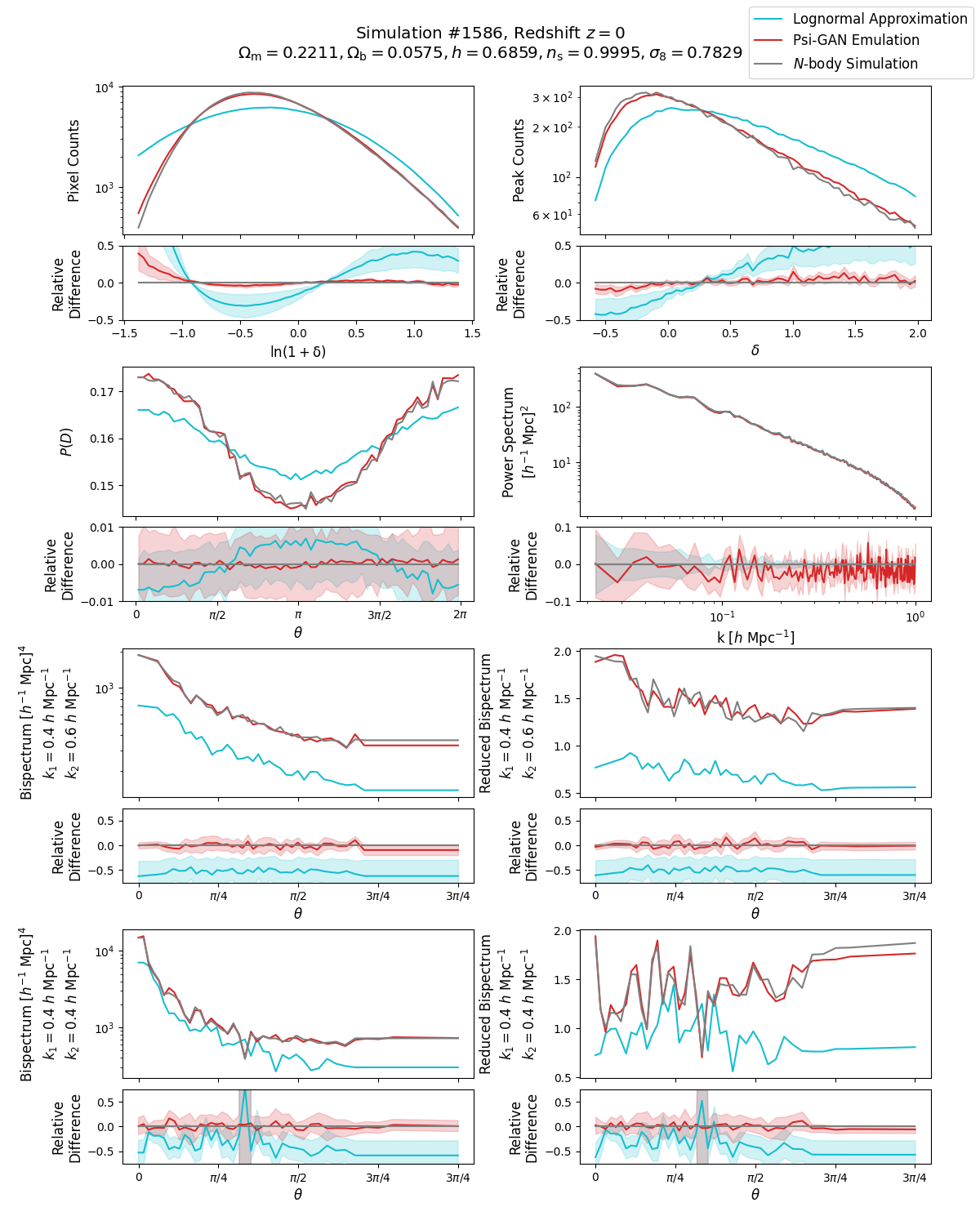
Figure 8: Similar to Figure 5, but for the test set for interpolating cosmology on simulation $\#1586$ at redshift $z=0$.

Figure 9 displays the relative differences for all redshifts tested (similar to Figure 6). Our second cosmology interpolation test for cosmology $\#815$ showed similar results to those shown for simulation $\#1586$.

Figure 9: Similar to Figure 6, but for the test set for interpolating cosmology on simulation $\#1586$.

Psi-GAN shows an improvement over the lognormal approximation, again with the sole exception of the power spectrum which was constrained so that it was not altered by more than ${\sim}5$ per cent. We do see greater discrepancies in the power spectrum compared to the previous tests. We believe that this discrepancy can be explained by the node coverage over cosmology-space when compared to redshift-space.

Redshift is a one-dimensional space which we cover with $5$ nodes at snapshots of $z\in\{0,0.5,1,2,3\}$. However, cosmology is a five-dimensional space (i.e. we condition on five cosmological parameters) which we cover with $2\,000$ nodes. In order to cover cosmology-space with the same density as we cover redshift-space, we would require $5^{5}=3\,125$ nodes in cosmology space. We are significantly short of this number, requiring $56.25$ per cent more simulations than are part of the Latin hypercube suite.

4.4 Model analysis through saliency mapping

Saliency mapping is a field of techniques used to produce visual explanations of the behaviour of computer vision models (Smilkov et al., 2017). These explanations take the form of heatmaps which aim to highlight which areas are most important for the model to reach a specific output. These scores are often computed by taking gradients of the output in question with regards to the input image (see e.g. Adebayo et al., 2018; Hooker et al., 2019, for an overview of various methods used in computer vision).

Saliency mapping has been explored in astrophysics through a variety of applications such as measuring galaxy bar lengths from morphology classification models (Bhambra et al., 2022), and qualitatively investigating model behaviour for both AGN classification models (Peruzzi et al., 2021) and cosmological parameter estimation models (Kacprzak & Fluri, 2022).

In order to investigate potential model improvements, we perform saliency mapping on the output of the critic with respect to a Psi-GAN emulation with the hope of discovering any features that may be tell-tale signs of a certain map being an emulation. We use SmoothGrad-Squared (Hooker et al., 2019) to visualise which areas of an emulation are used by the critic to identify it as an emulation as opposed to an $N$-body simulation.

SmoothGrad-Squared extends vanilla saliency (Simonyan et al., 2013), in which the saliency map $L^{c}$ is created by simply taking the gradient of the output with regards to each input pixel. Vanilla saliency has been shown to be unstable (Adebayo et al., 2018) due to gradients exhibiting large fluctuations with respect to pixel values, which creates excess noise in the resultant saliency maps. SmoothGrad-Squared aims to improve this limitation by creating $N_{\mathrm{sg}}$ visually similar samples of each image by adding a small amount of Gaussian noise to the original to create each sample, calculating a saliency map for each sample, and then aggregating these to produce a final saliency map:

$$\hat{L}^{c}(x)=\frac{1}{N_{\mathrm{sg}}}\sum^{N_{\mathrm{sg}}}_{i=1}L^{c}[x+\mathcal{N}(0,\sigma^{2})]^{2},$$ (16)

where $\mathcal{N}(0,\sigma^{2})$ is the probability density function for a Gaussian distribution with a mean of $0$ and a standard deviation of $\sigma^{2}$. Here we adopt the notation used by Hooker et al. (2019) in which $L^{c}$ is a vanilla saliency map, and $\hat{L}^{c}$ is the SmoothGrad-Squared saliency map that results from the squaring and aggregation of the saliency maps for each sample $x+\mathcal{N}(0,\sigma^{2})$. Throughout this section we use values of $N_{\mathrm{sg}}=256$ and $\sigma=0.2$ to control the number of samples, and the Gaussian noise used in the SmoothGrad-Squared algorithm, respectively.

Figure 10 shows an example at $z=0$ of an $N$-body simulation, a corresponding emulation produced by Psi-GAN, as well as the SmoothGrad-Squared saliency map, and a difference map.

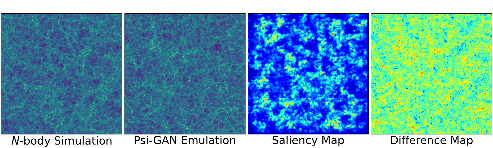
Figure 10: An example showing the the dark matter distribution field from an $N$-body simulation (left) and an emulation generated by Psi-GAN (centre left). We use SmoothGrad-Squared to produce a saliency map (centre right) visualising which parts of the emulation were most important for the critic when determining whether the emulation was real or fake. We also visualise the difference map (right), showing the differences between the $N$-body simulation and the Psi-GAN emulation.

We examined many such examples in order to visually identify any salient features that are highlighted in the saliency maps. However, we were unable to find any visual correlation between the saliency map and the other visualised maps. We assumed that this must be because the critic uses extremely small-scale features, or long-range correlations (which the human eye is poor at identifying) in order to differentiate Psi-GAN emulations and $N$-body simulations.

We also measure the power spectra of the saliency maps in order to investigate which scales are the limiting factor in Psi-GAN’s emulations. Figure 11 shows the power spectra for each redshift bin averaged over $64$ example maps and normalised such that the maximum value for each redshift is equal to $1$.

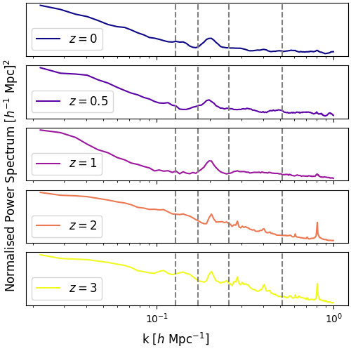
Figure 11: The normalised power spectra of SmoothGrad-Squared saliency maps evaluated on $64$ examples for each redshift snapshot for our “fiducial” cosmology. Vertical, dashed-grey lines indicate wavenumbers of integer multiples of the pixel width.

Taking the power spectra of the saliency maps shows us that Psi-GAN performs well over all scales. The power spectra show that long-range correlations are slightly more present in the saliency maps when compared to small-scale features. This indicates that Psi-GAN struggles to capture large scales in comparison to small scales, and that long-range correlations are the limiting factor in our architecture’s ability to accurately emulate the cosmic web.

We also see peaks at ${\sim}0.2~{}h~{}\mathrm{Mpc}^{-1}$ corresponding to a value of $2.5$ times the pixel width. This indicates that Psi-GAN exhibits small amounts of artefacting at small-scales. Although we do not have the computational resources to fully diagnose the cause of this, we believe that it is likely due to the interaction between the scale factor $2$ up-sampling and down-sampling used in the architecture, and the $9\times 9$ convolutional filter used in the ConvNeXt blocks (see Appendix A for further details). The convolutional filter propagates information from $4.5$ pixels away from the centre point of the central pixel, leading to the half-integer pixel width artefacting.

For redshifts $z=2$ and $z=3$ we also see a sharp peak at ${\sim}0.8~{}h~{}\mathrm{Mpc}^{-1}$. However, as this is on the sub-pixel scale we have no control over it, and we believe that its presence is due to the interpolation algorithm used by nbodykit when measuring the power spectrum.

5 Conclusions

In this paper, we used the Quijote simulations to train a machine learning model (Psi-GAN) capable of transforming two-dimensional flat-sky lognormal random fields of the dark matter overdensity field into more realistic samples across a continuous redshift and cosmology space. Psi-GAN takes the form of a generative adversarial network, with a U-Net generator and a novel critic which uses the power spectrum of the generated samples as a means for discrimination.

We have extensively tested Psi-GAN in a broad series of tests covering: the model’s training domain across all redshift ranges, the model’s ability to interpolate between the given redshift bins, and the model’s ability to interpolate between cosmologies at all redshifts. We observe that Psi-GAN has a closer agreement with $N$-body simulations when compared to the lognormal approximation across statistical tests that probe non-Gaussian features (such as peak counts, phase statistics, and bispectra). Psi-GAN is able to reproduce the bispectra and peak count distributions of $N$-body simulations to ${\sim}5$ per cent, while the lognormal approximation displays a discrepancy of ${\sim}25$ per cent. Due to our novel critic architecture, Psi-GAN is also able to match the power spectrum of the target $N$-body simulation, with relative differences of ${\sim}5$ per cent.

The largest shortcoming of Psi-GAN is its slightly weaker performance in constraining the power spectrum when tasked with interpolating between cosmologies. In our tests, the power spectrum of samples generated by Psi-GAN showed showed less agreement with $N$-body simulations when interpolating between the cosmologies used in the Quijote simulations. An approximately ${\sim}50$ per cent greater coverage of cosmology space should be enough to reduce this shortcoming, however this would require significant resources to generate. Another potential method of improving this would be to pre-train the model architecture to be able to reconstruct lognormal random fields across an extensive dataset before fine-tuning the model to transform lognormal random field to more accurate emulations.

We used saliency mapping techniques to investigate further architectural improvements to Psi-GAN, which highlighted a slight weakness in capturing long-range correlations as well as a small issue with pixel-scale artefacting. Increasing the depth of the generator by another step (i.e. including an extra set of down-sample and up-sample blocks) should help Psi-GAN model long-range correlations better as the latent space will be more compressed and information will propagate more efficiently across the simulation box. Adding additional ConvNeXt blocks after the first convolution, and before the last convolution should aid in modelling small scales and reduce artefacting.

Another architectural change that could improve performance is to replace the pre-trained ResNet-50 model in the critic with a more powerful option, such as the EfficientNet (Tan & Le, 2019) or RegNet (Radosavovic et al., 2020) architectures. However, all of these architectural changes will lead to a significant increase in training time which would require state-of-the-art hardware (although inference time should remain unchanged).

To meet our long-term goal of building a full-sky emulator to integrate into Glass, we will have to extend our work to the sphere. The Gower Street simulation suite (currently consisting of $791$ full-sky $N$-body simulations with varying cosmology; Jeffrey et al., 2024) provides us with a dataset for training, however it is not as extensive as the Quijote simulation suite used in this paper. Nevertheless, we see two potential avenues for future work on this problem: graph neural networks (see e.g. Lam et al., 2022, for an example pertaining to meteorology), and rotationally-equivariant convolutions on the sphere (see e.g. Ocampo et al., 2022; Boruah et al., 2024).

Carbon Intensity Statement

All work that went into this paper was tracked via “Weights and Biases”, which allows us calculate that we used a total of ${\sim}2\,000$ GPU hours throughout this work. The majority of this was on NVIDIA A100 Tensor Core GPUs, which had a time-averaged power consumption rate of ${\sim}0.19~{}\mathrm{kW}$ ($0.2~{}\mathrm{kW}$ during training and $0.1~{}\mathrm{kW}$ during validation and testing), thus resulting in a total power consumption of ${\sim}380~{}\mathrm{kW~{}h}$.

Using the average carbon intensity of the UK power grid in 2024 (measured at ${\sim}120~{}\mathrm{gCO_{2}eq}~{}\mathrm{kW^{-1}~{}h^{-1}}$; National Grid ESO, 2024), we estimate that we have emitted a total of ${\sim}45.6~{}\mathrm{kgCO_{2}eq}$ as the result of this work, roughly equivalent to that of a driving from London to Edinburgh and back (${\sim}1\,300~{}\mathrm{km}$) in a plug-in hybrid car.

We have removed the carbon emissions emitted due to this project from the atmosphere via the funding of carbon capture schemes through the Wren Trailblazer Portfolio.

Data Availability

All code required to reproduce this work has been made publicly available. The code includes a readme detailing the steps required to reproduce the study, including downloading all data and setting the seeds used when randomly splitting the datasets and augmenting training data. GitHub .

Appendix A Model architecture

Our generator consists of a ConvNeXt-inspired, conditional U-Net (Ronneberger et al., 2015), constructed from the four types of computational blocks shown in Figure 12. Our ConvNeXt block (Liu et al., 2022) consists of a depthwise separable $9\times 9$ convolution followed by two $1\times 1$ convolutions, as well as a residual connection. This architecture aims to efficiently process the input and share information across long ranges and is used as the main processing block for the generator. The conditioning block is used to inject information regarding the redshift and cosmology into the network. This is done by simply taking the $6$ conditioning labels ($z,\Omega_{\mathrm{m}},\Omega_{\mathrm{b}},h,n_{\mathrm{s}},\sigma_{8}$) and embedding them through a two-layered multi-level perceptron. We then expand the dimensions of the embeddings to match that of the input, before finally concatenating this with the input. The conditioning block has hyperparameters controlling the number of hidden and output nodes in the embedding network, which can be used to compress or expand the dimensions of the embedded labels. Following the ConvNeXt architecture, we have separated down-sampling and up-sampling operations away from the main computational block. The down-sample block consists of down-sampling the input using a $2\times 2$ convolution with a stride of $2$, and then processing the result with three sequential ConvNeXt blocks. The up-sample block takes two inputs, one from the previous step in the generator and another from a skip connection. The first input is up-sampled via bicubic interpolation with a scale-factor of $2$ to match the dimensions of the skip connection. These are then concatenated before being processed through a $3\times 3$ convolution, followed by three ConvNeXt blocks. Both the down-sample and up-sample blocks have a single parameter that controls the number of filters used in the initial convolution in each block. This is used to control the number of channels in the block’s output. Gaussian error linear units (GELU; Hendrycks & Gimpel, 2016) are used as activation functions throughout the construction of the network, and layer normalisation (LayerNorm; Lei Ba et al., 2016) is used for normalisation.

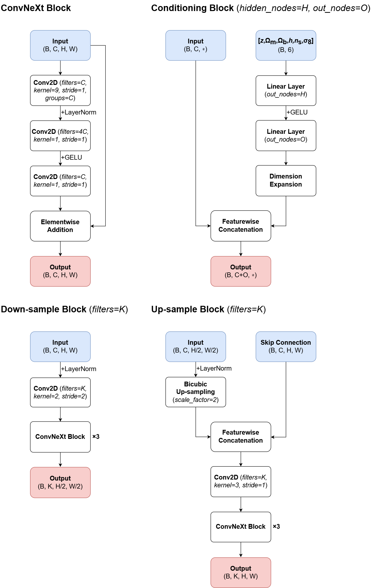
Figure 12: Schematics showing the four building blocks used in the construction of our generator and critic. We also provide information, in parentheses, regarding the dimensions for both the inputs (blue) and outputs (red) in roman font, and the hyperparameters of each layer and block in italics. Dimensions are quoted in the “batch, channels, $\ast$” convention, where $\ast$ represents any number of latent dimensions and (B, C, H, W) is used as a placeholder for the dimensions of two-dimensional inputs and outputs (with any lower-dimensional inputs and outputs following a similar convention). All convolutional layers use circular padding in order to maintain the height and width of the input.

The construction of the generator can be found in Figure 13. The generator consists of an initial $3\times 3$ convolution followed by three down-sample blocks. We then introduce a bottleneck consisting of three ConvNeXt blocks, before using three up-sample blocks to return the input to its original resolution. We use a final $1\times 1$ convolution to reduce the number channels back to $1$. We use conditioning blocks to inject information about redshift and cosmology before the initial and final convolutions, as well as before and after the bottleneck.

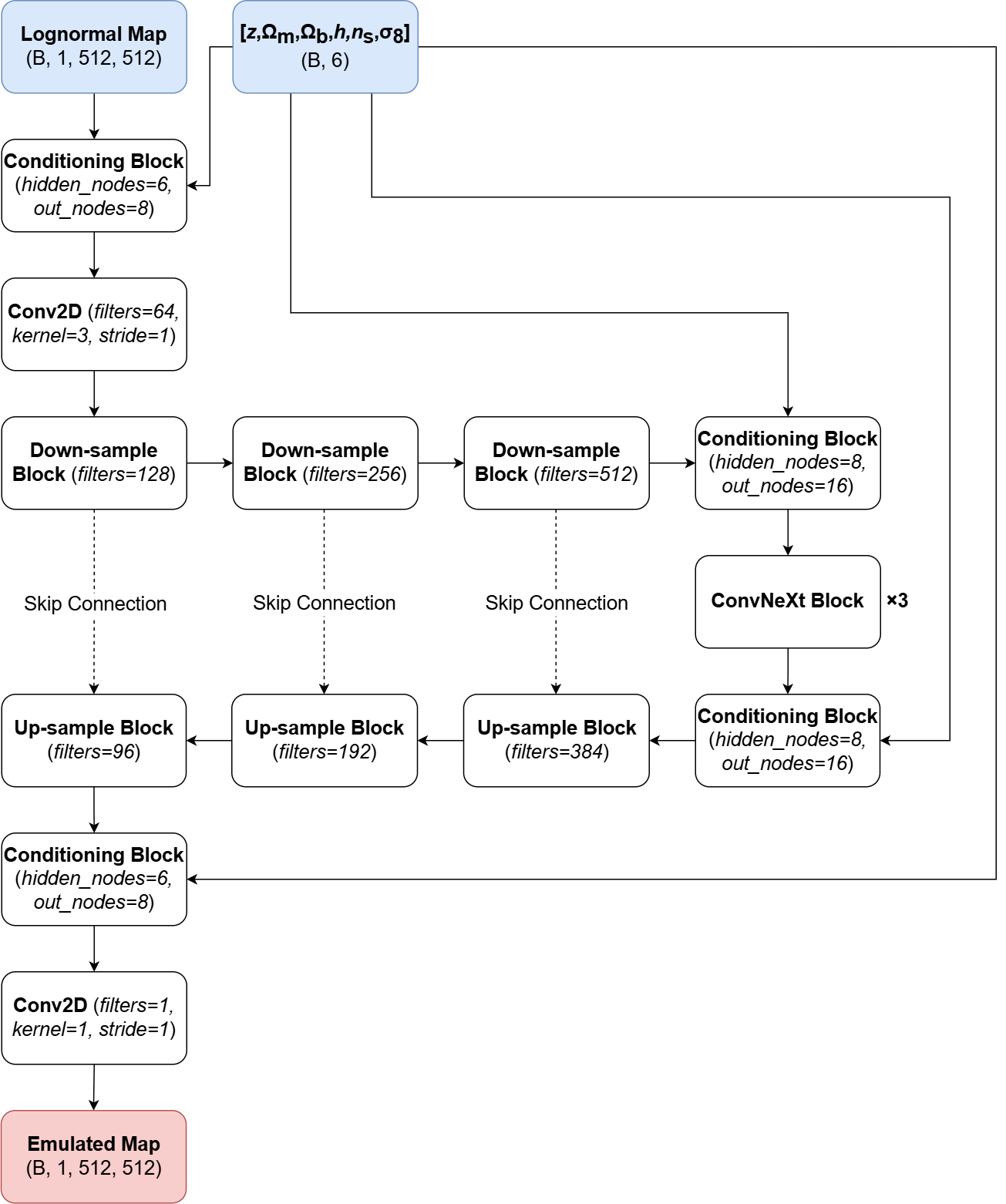
Figure 13: A schematic showing the construction of our conditional U-Net generator. We also provide information, in parentheses, regarding the dimensions for both the inputs (blue) and outputs (red) in roman font, and the hyperparameters of each layer in italics. Dimensions are quoted in the “batch, channels, $\ast$” convention, where $\ast$ represents any number of latent dimensions and B is used as a placeholder for the batch dimension of all inputs and outputs. All convolutional layers use circular padding in order to maintain the height and width of the input.

References

- Adebayo et al. (2018) Adebayo J., Gilmer J., Muelly M., Goodfellow I., Hardt M., Kim B., 2018, Advances in neural information processing systems, 31
- Arjovsky et al. (2017) Arjovsky M., Chintala S., Bottou L., 2017, in International conference on machine learning. pp 214–223
- Barnes & Hut (1986) Barnes J., Hut P., 1986, Nature, 324, 446
- Berge et al. (2010) Berge J., Amara A., Refregier A., 2010, The Astrophysical Journal, 712, 992
- Berger & Oliger (1984) Berger M. J., Oliger J., 1984, Journal of computational Physics, 53, 484
- Bertone & Hooper (2018) Bertone G., Hooper D., 2018, Reviews of Modern Physics, 90, 045002
- Bertone & Tait (2018) Bertone G., Tait T. M., 2018, Nature, 562, 51
- Bhambra et al. (2022) Bhambra P., Joachimi B., Lahav O., 2022, Monthly Notices of the Royal Astronomical Society, 511, 5032
- Blas et al. (2011) Blas D., Lesgourgues J., Tram T., 2011, Journal of Cosmology and Astroparticle Physics, 2011, 034
- Boruah et al. (2024) Boruah S. S., Fiedorowicz P., Garcia R., Coulton W. R., Rozo E., Fabbian G., 2024, arXiv preprint arXiv:2406.05867
- Boylan-Kolchin et al. (2009) Boylan-Kolchin M., Springel V., White S. D., Jenkins A., Lemson G., 2009, Monthly Notices of the Royal Astronomical Society, 398, 1150
- Bryan et al. (2014) Bryan G. L., et al., 2014, The Astrophysical Journal Supplement Series, 211, 19
- Chaniotis & Poulikakos (2004) Chaniotis A., Poulikakos D., 2004, Journal of Computational Physics, 197, 253
- Chiang & Coles (2000) Chiang L.-Y., Coles P., 2000, Monthly Notices of the Royal Astronomical Society, 311, 809
- Clerkin et al. (2017) Clerkin L., et al., 2017, Monthly Notices of the Royal Astronomical Society, 466, 1444
- Coles (2008) Coles P., 2008, in , Data Analysis in Cosmology. Springer, pp 493–522
- Coles & Chiang (2000) Coles P., Chiang L.-Y., 2000, Nature, 406, 376
- Coles & Jones (1991) Coles P., Jones B., 1991, Monthly Notices of the Royal Astronomical Society, 248, 1
- Coulton & Spergel (2019) Coulton W. R., Spergel D. N., 2019, Journal of Cosmology and Astroparticle Physics, 2019, 056
- Coulton et al. (2019) Coulton W. R., Liu J., Madhavacheril M. S., Böhm V., Spergel D. N., 2019, Journal of Cosmology and Astroparticle Physics, 2019, 043
- Cranmer et al. (2020) Cranmer K., Brehmer J., Louppe G., 2020, Proceedings of the National Academy of Sciences, 117, 30055
- Efstathiou et al. (1985) Efstathiou G., Davis M., White S., Frenk C., 1985, Astrophysical Journal Supplement Series, 57, 241
- Feder et al. (2020) Feder R. M., Berger P., Stein G., 2020, Physical Review D, 102, 103504
- Goodfellow et al. (2020) Goodfellow I., Pouget-Abadie J., Mirza M., Xu B., Warde-Farley D., Ozair S., Courville A., Bengio Y., 2020, Communications of the ACM, 63, 139
- Greengard & Rokhlin (1987) Greengard L., Rokhlin V., 1987, Journal of computational physics, 73, 325
- Gulrajani et al. (2017) Gulrajani I., Ahmed F., Arjovsky M., Dumoulin V., Courville A. C., 2017, Advances in neural information processing systems, 30
- Hand et al. (2018) Hand N., Feng Y., Beutler F., Li Y., Modi C., Seljak U., Slepian Z., 2018, The Astronomical Journal, 156, 160
- Harnois-Déraps et al. (2021) Harnois-Déraps J., Martinet N., Castro T., Dolag K., Giblin B., Heymans C., Hildebrandt H., Xia Q., 2021, Monthly Notices of the Royal Astronomical Society, 506, 1623
- Harnois-Deraps et al. (2024) Harnois-Deraps J., et al., 2024, arXiv preprint arXiv:2405.10312
- He et al. (2016) He K., Zhang X., Ren S., Sun J., 2016, in Proceedings of the IEEE conference on computer vision and pattern recognition. pp 770–778
- He et al. (2019) He S., Li Y., Feng Y., Ho S., Ravanbakhsh S., Chen W., Póczos B., 2019, Proceedings of the National Academy of Sciences, 116, 13825
- Hendrycks & Gimpel (2016) Hendrycks D., Gimpel K., 2016, arXiv preprint arXiv:1606.08415
- Heusel et al. (2017) Heusel M., Ramsauer H., Unterthiner T., Nessler B., Hochreiter S., 2017, Advances in neural information processing systems, 30
- Hockney & Eastwood (1988) Hockney R., Eastwood J., 1988, Computer Simulation Using Particles
- Hooker et al. (2019) Hooker S., Erhan D., Kindermans P.-J., Kim B., 2019, Advances in neural information processing systems, 32
- Jamieson et al. (2023) Jamieson D., Li Y., de Oliveira R. A., Villaescusa-Navarro F., Ho S., Spergel D. N., 2023, The Astrophysical Journal, 952, 145
- Jeffrey et al. (2024) Jeffrey N., et al., 2024, arXiv preprint arXiv:2403.02314
- Kacprzak & Fluri (2022) Kacprzak T., Fluri J., 2022, Physical Review X, 12, 031029
- Kacprzak et al. (2016) Kacprzak T., et al., 2016, Monthly Notices of the Royal Astronomical Society, 463, 3653
- Kingma & Ba (2014) Kingma D. P., Ba J., 2014, arXiv preprint arXiv:1412.6980
- Lam et al. (2022) Lam R., et al., 2022, arXiv preprint arXiv:2212.12794
- Lei Ba et al. (2016) Lei Ba J., Kiros J. R., Hinton G. E., 2016, preprint, pp arXiv–1607
- Lin & Kilbinger (2015a) Lin C.-A., Kilbinger M., 2015a, Astronomy & Astrophysics, 576, A24
- Lin & Kilbinger (2015b) Lin C.-A., Kilbinger M., 2015b, Astronomy & Astrophysics, 583, A70
- Lin et al. (2016) Lin C.-A., Kilbinger M., Pires S., 2016, Astronomy & Astrophysics, 593, A88
- Liu et al. (2022) Liu Z., Mao H., Wu C.-Y., Feichtenhofer C., Darrell T., Xie S., 2022, in Proceedings of the IEEE/CVF conference on computer vision and pattern recognition. pp 11976–11986
- Martinet et al. (2018) Martinet N., et al., 2018, Monthly Notices of the Royal Astronomical Society, 474, 712
- Matsubara (2003) Matsubara T., 2003, The Astrophysical Journal, 591, L79
- Matsubara (2007) Matsubara T., 2007, The Astrophysical Journal Supplement Series, 170, 1
- Mustafa et al. (2019) Mustafa M., Bard D., Bhimji W., Lukić Z., Al-Rfou R., Kratochvil J. M., 2019, Computational Astrophysics and Cosmology, 6, 1
- National Grid ESO (2024) National Grid ESO 2024, Historic generation mix and carbon intensity, https://www.nationalgrideso.com/data-portal/historic-generation-mix
- Ocampo et al. (2022) Ocampo J., Price M. A., McEwen J. D., 2022, arXiv preprint arXiv:2209.13603
- Peebles (1993) Peebles P. J. E., 1993, Principles of physical cosmology. Princeton Series in Physics Vol. 27, Princeton university press
- Percival et al. (2004) Percival W. J., Verde L., Peacock J. A., 2004, Monthly Notices of the Royal Astronomical Society, 347, 645
- Perraudin et al. (2019) Perraudin N., Srivastava A., Lucchi A., Kacprzak T., Hofmann T., Réfrégier A., 2019, Computational Astrophysics and Cosmology, 6, 1
- Peruzzi et al. (2021) Peruzzi T., Pasquato M., Ciroi S., Berton M., Marziani P., Nardini E., 2021, Astronomy & Astrophysics, 652, A19
- Piras et al. (2023) Piras D., Joachimi B., Villaescusa-Navarro F., 2023, Monthly Notices of the Royal Astronomical Society, 520, 668
- Pires et al. (2012) Pires S., Leonard A., Starck J.-L., 2012, Monthly Notices of the Royal Astronomical Society, 423, 983
- Radosavovic et al. (2020) Radosavovic I., Kosaraju R. P., Girshick R., He K., Dollár P., 2020, in Proceedings of the IEEE/CVF conference on computer vision and pattern recognition. pp 10428–10436
- Rodríguez et al. (2018) Rodríguez A. C., Kacprzak T., Lucchi A., Amara A., Sgier R., Fluri J., Hofmann T., Réfrégier A., 2018, Computational Astrophysics and Cosmology, 5, 1
- Ronneberger et al. (2015) Ronneberger O., Fischer P., Brox T., 2015, in Medical image computing and computer-assisted intervention–MICCAI 2015: 18th international conference, Munich, Germany, October 5-9, 2015, proceedings, part III 18. pp 234–241
- Scoccimarro (2000) Scoccimarro R., 2000, The Astrophysical Journal, 544, 597
- Sefusatti et al. (2006) Sefusatti E., Crocce M., Pueblas S., Scoccimarro R., 2006, Physical Review D, 74, 023522
- Sefusatti et al. (2016) Sefusatti E., Crocce M., Scoccimarro R., Couchman H., 2016, Monthly Notices of the Royal Astronomical Society, 460, 3624
- Shan et al. (2018) Shan H., et al., 2018, Monthly Notices of the Royal Astronomical Society, 474, 1116
- Shirasaki & Ikeda (2023) Shirasaki M., Ikeda S., 2023, arXiv preprint arXiv:2310.17141
- Simonyan et al. (2013) Simonyan K., Vedaldi A., Zisserman A., 2013, arXiv preprint arXiv:1312.6034
- Smilkov et al. (2017) Smilkov D., Thorat N., Kim B., Viégas F., Wattenberg M., 2017, arXiv preprint arXiv:1706.03825
- Springel (2005) Springel V., 2005, Monthly Notices of the Royal Astronomical Society, 364, 1105
- Springel et al. (2005) Springel V., et al., 2005, Nature, 435, 629
- Springel et al. (2021) Springel V., Pakmor R., Zier O., Reinecke M., 2021, Monthly Notices of the Royal Astronomical Society, 506, 2871
- Tan & Le (2019) Tan M., Le Q., 2019, in International conference on machine learning. pp 6105–6114
- Tessore et al. (2023) Tessore N., Loureiro A., Joachimi B., von Wietersheim-Kramsta M., Jeffrey N., 2023, The Open Journal of Astrophysics, 6, 11
- Villaescusa-Navarro et al. (2020) Villaescusa-Navarro F., et al., 2020, The Astrophysical Journal Supplement Series, 250, 2
- Villaescusa-Navarro et al. (2021) Villaescusa-Navarro F., et al., 2021, The Astrophysical Journal, 915, 71
- Watts et al. (2003) Watts P., Coles P., Melott A., 2003, The Astrophysical Journal, 589, L61
- Xavier et al. (2016) Xavier H. S., Abdalla F. B., Joachimi B., 2016, Monthly Notices of the Royal Astronomical Society, 459, 3693
- Zhu et al. (2017) Zhu J.-Y., Park T., Isola P., Efros A. A., 2017, in Proceedings of the IEEE international conference on computer vision. pp 2223–2232
- Zürcher et al. (2022) Zürcher D., et al., 2022, Monthly Notices of the Royal Astronomical Society, 511, 2075
- de Oliveira et al. (2020) de Oliveira R. A., Li Y., Villaescusa-Navarro F., Ho S., Spergel D. N., 2020, arXiv preprint arXiv:2012.00240
- von Wietersheim-Kramsta et al. (2024) von Wietersheim-Kramsta M., Lin K., Tessore N., Joachimi B., Loureiro A., Reischke R., Wright A. H., 2024, arXiv preprint arXiv:2404.15402