BBN Constraint on Heavy Neutrino Production and Decay

Abstract

We explore the big-bang nucleosynthesis (BBN) constraint on heavy neutrino that is a mixture of gauge singlet fermion and active neutrinos in the Standard Model. We work in the minimal model with only two parameters, the heavy neutrino mass $m_{4}$ and the mixing parameter $|U_{a4}|^{2}$, where $a=e$, $\mu$, or $\tau$ stands for the active neutrino flavor. We show that both the early universe production mechanism and decay products of the heavy neutrino are determined by $m_{4}$ and $|U_{a4}|^{2}$, with little room for further assumptions. This predictivity allows us to present a portrait of the entire BBN excluded parameter space. Our analysis includes various effects including temporary matter domination, energy injections in the form of pions, photons and light neutrinos. The BBN constraint is complementary to terrestrial search for heavy neutrinos (heavy neutral leptons) behind the origin of neutrino masses and portal to the dark sector.

1 Introduction

The neutrino sector of the Standard Model hosts a number of opportunities for new physics searches. The phenomena of neutrino oscillations reveal that neutrinos have nonzero masses and mixings, which require beyond the Standard Model physics [1, 2, 3]. Through the type-I seesaw mechanism [4, 5, 6, 7, 8], neutrinos obtain their masses by coupling to gauge-singlet sterile neutrinos that are Majorana fermions. This scenario could be tested at low energies in lepton number violating processes such as neutrinoless double beta decay [9, 10, 11, 12, 13, 14], and by hunting the heavy neutrino as novel, elusive particles using terrestrial and cosmological experiments [15, 16, 17, 18, 19, 20, 21, 22, 23, 24, 25, 26, 27, 28, 29, 30]. Besides neutrino mass generation models, heavy right-handed neutrinos (as Majorana or Dirac fermions) are often considered as a portal to dark sectors which accommodate dark matter particles that fill the universe [31, 32, 33, 34, 35].

The big-bang nucleosynthesis (BBN) provides a unique lens into the very early universe for exploring the Standard Model and beyond [36, 37, 38, 39]. The fact that BBN predictions of primordial element abundances agree well with the observations in standard cosmology limits the room of new physics, including the equation of state and expansion rate of the universe, as well as exotic energy injections. These effects could occur if a population of heavy neutrinos decays into Standard Model particles during the BBN epoch [40, 41, 42, 43, 44]. In a number of recent studies, the BBN constraints are presented as an upper bound on the heavy neutrino’s lifetime, or a lower bound on the active-sterile neutrino mixing, by assuming that the heavy neutrino decouples from thermal equilibrium in early universe [45, 46, 47, 48, 49, 50].

In this article, we take minimality as the guiding principle and explore simplified models where the mixing of sterile neutrino with the Standard Model active neutrino is the only portal for it to interact with other known particles. Under this assumption, there is little ambiguity in the fate of heavy neutrino in the early universe. We consider the mixing involves one active neutrino flavor in each case, so that the production and decay of heavy neutrino is essentially dictated by two parameters, the heavy neutrino’s mass and its mixing with the active neutrino.

The interplay between the heavy neutrino lifetime and its thermal contact with the Standard Model plasma is a useful guideline for our study. Note that only sufficiently weakly-coupled heavy neutrino with a small mixing parameter can have a lifetime comparable to the BBN time scale. For sufficiently small mixing, the heavy neutrino may not establish thermal equilibrium with the Standard Model particles. To set the most conservative limit, we assume it begins with zero initial population after inflation and any abundance must be built up through the mixing with active neutrinos. The BBN constraint on heavy neutrino can be evaded if the mixing parameter is tiny so that the heavy neutrino is rarely produced, or if the mixing is so large that the heavy neutrino decays away well before one second. As a result, the BBN constraint only applies to a window of intermediate mixing values. The goal of this work is to quantify the position of this window as a function of the heavy neutrino mass.

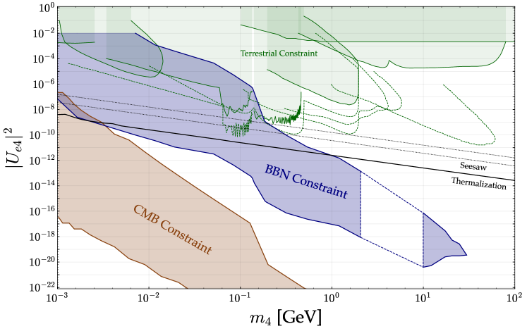
Figure 1: BBN (blue shaded region) and CMB (brown shaded region) constraints derived in this work on the parameter space of heavy neutrino mass versus its mixing with the active neutrino (electron flavor in this case). For BBN, the gap of $m_{4}$ between a few and 10 GeV is not shaded with blue where our computation is limited by the complexity of QCD. The black dotted lines show the mixing angles when heavy neutrinos explain the active neutrino mass via the seesaw mechanism described in Eq. (1.4). In the region above the black solid curve, the heavy neutrino can reach thermal equilibrium with the Standard Model plasma in the early universe (see Fig. 2). We also show other laboratory constraints for comparison, including the current (green shaded region) and future (green dashed line) limits.

To set the stage, we introduce the minimal model of heavy neutrino that contains a mixture of the active neutrino component. The heavy neutrino mass eigenstate is a linear combination of a gauge singlet fermion $\nu_{s}$ (sterile neutrino) and active neutrino $\nu_{a}$. In the vacuum,

$$\nu_{4}\simeq\nu_{s}+U_{a4}\nu_{a}\ ,$$ (1.1)

where $U_{a4}$ is a matrix element of the neutrino mixing matrix, and $|U_{a4}|$ is much smaller than unity due to existing constraints (see below). Both $\nu_{s}$ and $\nu_{a}$ are flavor eigenstates that can be distinguished by weak interactions. In general, the $\nu_{a}$ here could be a linear combination of three active neutrino flavors. In this work, we consider a singlet flavor for simplicity in each analysis. The mass of $\nu_{4}$ we are interested in lies in the range of MeV to the weak scale. In contract, the orthogonal mass eigenstates $\nu_{1,2,3}$ are constrained to be lighter than $\sim 0.1$ eV [51, 52].

Through the above mixing, the mass eigenstate $\nu_{4}$ can participate in weak interactions mediated by the $W,Z$ bosons, with couplings suppressed by the small $U_{a4}$,

$$\mathcal{L}_{\rm int}=\frac{eU_{a4}}{\sqrt{2}\sin\theta_{w}}\bar{\ell}_{a}\gamma^{\mu}\mathbb{P}_{L}\nu_{4}W^{-}_{\mu}+\frac{eU_{a4}}{\sin(2\theta_{w})}\bar{\nu}_{a}\gamma^{\mu}\mathbb{P}_{L}\nu_{4}Z_{\mu}+{\rm h.c.}\ ,$$ (1.2)

where $\theta_{w}$ is the Weinberg angle and $e$ is the electric charge unit. These interactions are important for studying the decay of heavy neutrinos.

Taking the type-I seesaw mechanism [4, 7] as a concrete example, the mixing in Eq. (1.1) can be generated by the following Lagrangian

$$\mathcal{L}_{\rm seesaw}=\frac{1}{2}\left(\bar{N}i\cancel{\partial}N+M\bar{N}N\right)+\left(y\bar{L}_{a}H\nu_{s}+{\rm h.c.}\right)\ ,$$ (1.3)

where $N=\nu_{s}+\nu_{s}^{c}$, and $\nu_{s}=\mathbb{P}_{R}N$ is the right-handed neutrino. $L_{a}$ and $H$ are the lepton and Higgs doublets. After electroweak symmetry breaking, $\langle H\rangle=v/\sqrt{2}$, the active-sterile neutrino mixing parameter is given by

$$U_{a4}\simeq\frac{yv}{\sqrt{2}M}\simeq\sqrt{\frac{m^{\nu}_{\rm light}}{M}}\ ,$$ (1.4)

and the mass eigenvalue for the heavy, mostly sterile state is $m_{4}\simeq M$. On the other hand, in neutrino portal dark sector models, the mixing parameter $|U_{a4}|$ is not necessarily tied to the neutrino mass and allowed to take a broader range of values.

Fig. 1 presents the main results of this work, for heavy neutrino mixing with $\nu_{e}$. (Results for mixing with $\nu_{\mu},\nu_{\tau}$ are in Fig. 9.) The two gray dotted lines indicate the typical active-sterile neutrino mixing values in the type-I seesaw mechanism for generating the atmospheric and solar neutrino mass differences. The BBN constraints are shown by the blue shaded region. Clearly they have a large overlap with the seesaw target for explaining the light neutrino masses and they are highly complementary to the terrestrial experiments which probe the higher $|U_{a4}|^{2}$ values (green shaded regions).  For given heavy neutrino mass $m_{4}$ (horizontal axis), the BBN exclusion applies for a window of the mixing parameter $|U_{a4}|^{2}$. In the parameter space above the blue region, the heavy neutrino decays very early and the effects on BBN are opaqued away by the thermal plasma. In contrast, in the parameter space below the blue region, the heavy neutrino is long-lived and decays during the BBN epoch. However, the mixing parameter is so small that no thermal contact is reached between the heavy neutrino and the Standard Model sector, and the freeze-in abundance is too small to affect the primordial element abundances. In that region, we show a constraint from the cosmic microwave background (CMB) due to excessive energy injections from the decay of heavy neutrino.

2 Heavy Neutrino Production in the Early Universe

We first address the production of heavy neutrinos in the early universe. The black solid line in Fig. 1 divides the parameter space into two parts. In the large $|U_{a4}|^{2}$ region above the line, heavy neutrinos are populated via the regular thermal freeze out mechanism, whereas in the small $|U_{a4}|^{2}$ region the production is freeze in via neutrino oscillation processes [40, 41, 42, 43, 44].

An important player in both production mechanisms is the effective mixing angle between the active and sterile neutrinos. In the early universe plasma, this mixing is modified from its vacuum value in Eq. (1.1) due to weak interactions acting on the active neutrino state. This manifests as a potential term that alters neutrino’s dispersion relation and a scattering rate acting as a damping effect to the oscillation process. Both effects are temperature dependent. The active-to-sterile neutrino oscillation problem can be described starting from the quantum kinetic equation of the density matrix [53]. In the limit where the weak interaction has a much larger rate than the expansion of the universe (i.e., $T\gg\,{\rm MeV}$), the set of density matrix equations can be simplified to a simple Boltzmann equation that governs the phase space distribution (PSD) function of sterile neutrino,

$$\frac{\partial f_{s}(x,a)}{\partial\ln a}=\frac{\Gamma\sin^{2}(2\theta_{\rm eff})}{4H}(f_{\rm eq}-f_{s})\ .$$ (2.1)

We refer to the appendix A for more details. Here, the argument of the differential equation $a$ is the scale factor of the universes, $H=\dot{a}/a$ is the Hubble parameter, and

$$f_{\rm eq}(x)=\frac{1}{1+e^{x}}\ ,$$ (2.2)

is the Fermi-Dirac distribution function, $x=E/T$, and $E$ is the oscillating neutrino energy. The production of sterile neutrino occurs when it is still ultra-relativistic, thus $x$ is time (temperature) independent. In the early universe plasma, the effective mixing angle between active and sterile neutrino is

$$\sin^{2}(2\theta_{\rm eff})=\frac{\Delta^{2}\sin^{2}(2\theta)}{\Delta^{2}\sin^{2}(2\theta)+\left(\Delta\cos(2\theta)-V\right)^{2}+(\Gamma/2)^{2}}\ .$$ (2.3)

Here $\theta$ is the vacuum mixing angle and approximately equals to $|U_{a4}|$ introduced in Eq. (1.1), thus

$$\sin(2\theta)\simeq 2|U_{a4}|\ ,\quad\cos(2\theta)\simeq 1\ .$$ (2.4)

On the right-hand side of Eq. (2.1), the quantities $\Delta,V,\Gamma$ are all functions of $x$ and $a$. $\Delta=m_{4}^{2}/(2E)$ is the vacuum oscillation frequency, and the thermal potential for active neutrino is [54]

$$V=-\frac{7\sqrt{2}\pi^{2}G_{\rm F}ET^{4}}{45}\left(\frac{2}{M_{W}^{2}}+\frac{1}{M_{Z}^{2}}\right)\ .$$ (2.5)

For simplicity, we assume zero neutrino chemical potential (asymmetry) throughout this work.

The total reaction rate $\Gamma$ for an active neutrino state with energy $E$ sums over all the processes involving the active neutrino and the ambient particles in the thermal plasma. At temperatures well below the weak scale, it takes the form

$$\Gamma=c_{\nu}G_{F}^{2}ET^{4}\ .$$ (2.6)

The value of coefficient $c_{\nu}$ depends on the temperature and the flavor of active neutrino that mixes with the sterile neutrino, and is given in the following table. At $T<m_{e}$, the coefficient $c_{\nu_{e}}=7\pi/24$ was used in [44]. Going to higher temperatures, the coefficient $c_{\nu}$ is enhanced by the multiplicity of particle species in the thermal plasma. At given $T$, we derive the $c_{\nu}$ value by neglecting light fermion masses ($m_{f}<T$) and decoupling the heavy ones.

 T<me7​π277​π277​π27 me<T<mμ91​π2167​π247​π24 mμ<T<ΛQ​C​D77​π10877​π10835​π108 ΛQ​C​D<T<mc203​π108203​π10877​π108 mc<T<mτ244​π81244​π81133​π162 mτ<T<mb1981​π6481981​π6481981​π648 T>mb259​π81259​π81259​π81subscript𝑐𝜈fragments fragments Tm𝑒7𝜋277𝜋277𝜋27fragments m𝑒Tm𝜇91𝜋2167𝜋247𝜋24fragments m𝜇TΛ𝑄𝐶𝐷77𝜋10877𝜋10835𝜋108fragments Λ𝑄𝐶𝐷Tm𝑐203𝜋108203𝜋10877𝜋108fragments m𝑐Tm𝜏244𝜋81244𝜋81133𝜋162fragments m𝜏Tm𝑏1981𝜋6481981𝜋6481981𝜋648fragments Tm𝑏259𝜋81259𝜋81259𝜋81c_{\nu}=\begin{tabular}[]{| c | c | c | c |}\hline\cr{temperature range}&$\nu_{e}$&$\nu_{\mu}$&$\nu_{\tau}$\\ \hline\cr\rule{0.0pt}{15.0pt} $T<m_{e}$&$\frac{7\pi}{27}$&$\frac{7\pi}{27}$&$\frac{7\pi}{27}$\\[2.15277pt] \hline\cr\rule{0.0pt}{15.0pt} $m_{e}<T<m_{\mu}$&$\frac{91\pi}{216}$&$\frac{7\pi}{24}$&$\frac{7\pi}{24}$\\[2.15277pt] \hline\cr\rule{0.0pt}{15.0pt} $m_{\mu}<T<\Lambda_{QCD}$&$\frac{77\pi}{108}$&$\frac{77\pi}{108}$&$\frac{35\pi}{108}$\\[2.15277pt] \hline\cr\rule{0.0pt}{15.0pt} $\Lambda_{QCD}<T<m_{c}$&$\frac{203\pi}{108}$&$\frac{203\pi}{108}$&$\frac{77\pi}{108}$\\[2.15277pt] \hline\cr\rule{0.0pt}{15.0pt} $m_{c}<T<m_{\tau}$&$\frac{244\pi}{81}$&$\frac{244\pi}{81}$&$\frac{133\pi}{162}$\\[2.15277pt] \hline\cr\rule{0.0pt}{15.0pt} $m_{\tau}<T<m_{b}$&$\frac{1981\pi}{648}$&$\frac{1981\pi}{648}$&$\frac{1981\pi}{648}$\\[2.15277pt] \hline\cr\rule{0.0pt}{15.0pt} $T>m_{b}$&$\frac{259\pi}{81}$&$\frac{259\pi}{81}$&$\frac{259\pi}{81}$\\[2.15277pt] \hline\cr\end{tabular}

temperature rangeνeνμντtemperature rangeνeνμντ (2.7)

Based on Eq. (2.1), whether the sterile neutrino state could reach thermal equilibrium is dictated by the ratio $\Gamma_{a}\sin^{2}(2\theta_{\rm eff})/H$. Consider a neutrino with average energy $E\sim T$ in the radiation dominated universe, the weak interaction rate and Hubble have simple scaling with the temperature, $\Gamma\sim G_{F}^{2}T^{5}$ and $H\sim T^{2}$. On the other hand, the effective mixing angle $\sin^{2}(2\theta_{\rm eff})$ has a less trivial temperature dependence. At high temperatures when $\Gamma,V\gg\Delta$, the effective mixing angle is suppressed by weak interactions compared to the vacuum value, and we have $\sin^{2}(2\theta_{\rm eff})\sim\Delta^{2}|U_{a4}|^{2}/\Gamma^{2}\sim T^{-12}$. As the universe cools, $\Gamma_{a}$ and $V_{a}$ decrease whereas $\Delta$ grows; $\theta_{\rm eff}$ eventually settles down to $\theta\simeq|U_{a4}|$. This interplay defines a critical temperature $T_{*}$, with

$$T_{*}\simeq\left(\frac{m_{4}}{G_{F}}\right)^{1/3}\simeq 45\,{\rm GeV}\left(\frac{m_{4}}{1\,{\rm GeV}}\right)^{1/3}\ ,$$ (2.8)

defined by $\Gamma\simeq\Delta$. The ratio $\Gamma\sin^{2}(2\theta_{\rm eff})/H$ is largest at temperature $T_{*}$, and suppressed at both very large and very small temperatures,

$$\frac{\Gamma\sin^{2}(2\theta_{\rm eff})}{H}\propto\left\{\begin{array}[]{cl}T^{-9},&\quad T>T_{*}\\ T^{3},&\quad T<T_{*}\end{array}\right.$$ (2.9)

The peak at $T_{*}$ corresponds to the epoch where the sterile neutrino has the most thermal contact with the Standard Model sector. It is worth noting that for $m_{4}$ below the electroweak scale, $T_{*}$ is always much larger than the sterile neutrino mass $m_{4}$.

2.1 Freeze-out Production

If $\Gamma\sin^{2}(2\theta_{\rm eff})/H>1$ at temperature $T_{*}$, the sterile neutrino state will reach thermal equilibrium with the Standard Model plasma for a period around $T_{*}$. This requires

$$|U_{a4}|^{2}\gtrsim\frac{1}{G_{F}M_{\rm P}m_{4}}\simeq 10^{-14}\left(\frac{1\,\rm GeV}{m_{4}}\right)\ ,$$ (2.10)

where $M_{\rm P}=1.2\times 10^{19}$ GeV is the Planck scale.

As the universe cools, it eventually drops out of equilibrium when the ratio $\Gamma\sin^{2}(2\theta_{\rm eff})/H$ drops to around unity. The freeze out temperature can be estimated to be

$$T_{\rm fo}\simeq\left(G_{F}^{2}M_{\rm P}|U_{a4}|^{2}\rule{0.0pt}{11.38109pt}\right)^{-1/3}\ .$$ (2.11)

In practice, we find that sterile neutrino always freezes out relativistically for the range of parameter space constrained by BBN. Indeed, the condition for relativistic freeze out $T_{\rm fo}>m_{4}$ amounts to

$$|U_{a4}|^{2}\lesssim\frac{1}{G_{F}^{2}M_{\rm P}m_{4}^{3}}\simeq 10^{-4}\left(\frac{1\,\rm GeV}{m_{4}}\right)^{3}\ .$$ (2.12)

This upper bound is consistent with the freeze out condition Eq. (2.10) for sterile neutrino mass below the electroweak scale.

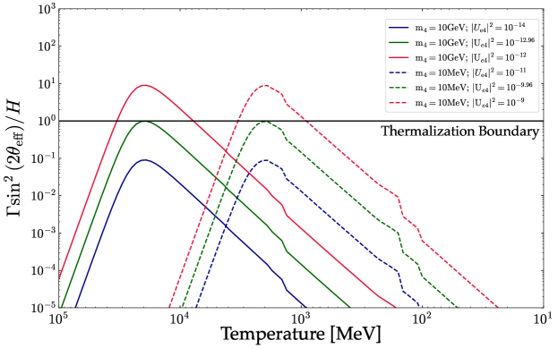
Figure 2: The ratio between the total interaction rate of heavy neutrino in the early universe and the Hubble expansion rate as a function of temperature, for two choices of $m_{4}$ and various mixing parameter $|U_{\alpha 4}|^{2}$. Thermalization occurs when the ratio is larger than 1. For both solid and dashed curves, red (blue) corresponds to freeze-out (-in) production, and green shows the marginal case.

2.2 Freeze-in Production

If $\Gamma\sin^{2}(2\theta_{\rm eff})/H\ll 1$ at temperature $T_{*}$, the sterile neutrino is never in thermal equilibrium with the Standard Model sector. In this case, its abundance is given by the freeze in mechanism plus an initial condition. We can directly integrate Eq. (2.1) by dropping the $f_{s}$ term on the right-hand side

$$\frac{\partial f_{s}(x,a)}{\partial\ln a}\simeq\frac{\Gamma\sin^{2}(2\theta_{\rm eff})}{4H}f_{\rm eq}\ .$$ (2.13)

The sterile neutrino is dominantly produced at temperature $T_{*}$. As argued above, $T_{*}$ is always higher than $m_{4}$. Therefore, the production occurs in the same way as the Dodelson-Widrow mechanism for keV-scale sterile neutrino dark matter production. In Fig. 2, we plot $\Gamma\sin^{2}(2\theta_{\rm eff})/H$ as a function of the temperature (time), for three different value of $|U_{a4}|^{2}$. The red, blue, green curves corresponds to freeze-out, freeze-in production, and the marginal cases.

A subtle point to clarify is that the sterile neutrino from oscillation is first produced as a pure $\nu_{s}$ flavor eigenstate (see Eq. (2.1)), but to discuss decays we must work in the mass basis. In the $|U_{a4}|^{2}\ll 1$ limit, there is no need to distinguish between the two. Nearly 100% of $\nu_{s}$ ends up in the heavy neutrino mass eigenstate $\nu_{4}$. The probability for $\nu_{s}$ to oscillate once more is suppressed by another $|U_{a4}|^{2}$.

After the completion of freezing out or freeze in, the number density of sterile neutrinos simply drops as $a^{-3}$ with the expansion of the universe until decay takes place.

2.3 Temporary matter domination

The heavy neutrinos made in early universe can impact BBN in several ways. We first discuss an effect prior to the decay taking place. The heavy neutrinos are produced relativistically but later become matter-like. Before decaying away, its energy density redshifts slower than the radiation fluids made of SM particles and could potentially come into temporary domination of the total energy in the universe. Fig. 3 (left) shows the energy density evolution for the heavy neutrino and radiation, for three different mass and mixing combinations. Temporary matter domination occurs for the light magenta curve. In our calculation, the Hubble parameter is controlled by the sum of $\rho_{4}$ and $\rho_{R}$.

The red curve in Fig. 3 (right) shows the mixing parameter $|U_{a4}|^{2}$ allowing for the temporary matter domination, along with the black curve on which the lifetime of $\nu_{4}$ equals one second. See also Fig. 6 and discussions therein.

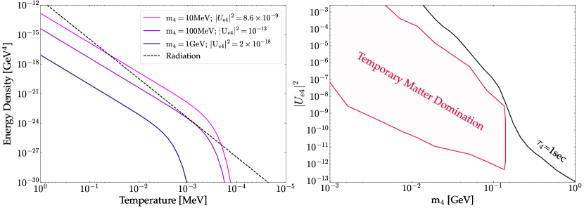
Figure 3: Left panel: Energy density of heavy neutrino as a function of temperature. We show three scenarios where the universe is temporarily dominated by heavy neutrino (magenta), always radiation dominated (navy), and the marginal case (violet) The black dashed line is the radiation energy density in the standard cosmology. Right panel: We show the minimal mixing parameter $|U_{a4}|^{2}$ for the temporary matter domination curve (red) and the lifetime equals one second curve (black) on the parameter space of heavy neutrino mass versus mixing. The region enclosed by two curves is roughly where the BBN exclusion of temporary matter domination applies.

Departure from radiation domination modifies the clock of the universe during BBN, and is tightly constrained [55]. We require that the heavy neutrino has never dominated the energy density of the universe during BBN, i.e.,

$$\rho_{4}<\rho_{R}\ ,\quad\text{for all }\hskip 8.5359ptt\geq 1\,{\rm sec}\ ,$$ (2.14)

where

$$\rho_{4}=\int\frac{d^{3}p}{(2\pi)^{3}}\sqrt{p^{2}+m_{4}^{2}}f_{s}\left(\sqrt{p^{2}+m_{4}^{2}}/T\right)\ ,\quad\rho_{R}=\frac{\pi^{2}}{30}g_{*}(T)T^{4}\ ,$$ (2.15)

and $f_{s}$ is the PSD function calculated above for the freeze-out or freeze-in mechanisms. Before the decay taking place, we have $\rho_{4}\sim a^{4(3)}$ for $T\gg(\ll)\,m_{4}$, where $a$ is the scale factor of the universe. Obeying Eq. (2.14) ensures that BBN occurs in an entirely radiation dominated universe.

3 Heavy Neutrino Decay During BBN

For the range of parameters considered in this work, the heavy neutrinos are always produced relativistically in both the freeze out and freeze in scenarios. They share a similar temperature to the Standard Model plasma and would become non-relativistic when the temperature falls below their mass $m_{4}$. In this work, we will focus on the mass range $m_{4}>{\rm MeV}$ and explore the decay effects on BBN at temperatures below MeV. Therefore, for the entire parameter space of interest to this study, the sterile neutrinos are produced relativistically but decay after they have become non-relativistic. There is always sufficient expansion of the universe for the transition to occur.

Thanks to this separation of scales, we can simply account for the heavy neutrino decay by multiplying an exponential decay factor to its number density. The number density at late time is given by

$$n_{\nu_{4}}(t)=n_{\nu_{4}}(t_{i})\left(\frac{a(t_{i})}{a(t)}\right)^{3}\exp\left(-\frac{\Gamma_{\nu_{4}}^{\rm tot}}{2H}\right)\ ,$$ (3.1)

where $\Gamma_{\rm tot}$ is the total decay rate of heavy neutrino $\nu_{4}$ and $t_{i}$ is a time chosen to be well after the production and well before the decay. In radiation dominated universe, $t=1/(2H)$.

The decays of heavy neutrino include leptonic and semi-leptonic modes. Neglecting the final state particle masses, the partial decay width in the rest frame of a light $\nu_{4}$ takes the generic form

$$\Gamma_{\nu_{4}\to X}=\tilde{c}_{\nu_{4}\to X}\dfrac{G_{F}^{2}m_{4}^{5}}{\pi^{3}}|U_{a4}|^{2}\ .$$ (3.2)

From Eq. (2.8), we find that $T_{*}$ is always much larger than the BBN temperatures, for the mass range $m_{4}>{\rm MeV}$ we will consider. Therefore, the active-sterile mixing angle governing the decay takes the vacuum value to a very good approximation.

The decay coefficients for leptonic decay modes are

$$\begin{split}\tilde{c}_{\nu_{4}\to\nu_{a}\nu_{a}\bar{\nu}_{a}}&=\frac{1}{192}\ ,\quad\tilde{c}_{\nu_{4}\to\nu_{a}\ell^{+}_{a}\ell^{-}_{a}}=\frac{5}{768}\ ,\\ \tilde{c}_{\nu_{4}\to\nu_{a}\nu_{b}\bar{\nu}_{b}}&=\frac{1}{96}\ ,\quad\tilde{c}_{\nu_{4}\to\nu_{a}\ell^{+}_{b}\ell^{-}_{b}}=\frac{1}{768}\ ,\quad\tilde{c}_{\nu_{4}\to\nu_{b}\ell^{+}_{b}\ell^{-}_{a}}=\frac{1}{768}\ ,\\ \end{split}$$ (3.3)

Here the flavor indices are not summed over, we assume that $\nu_{4}$ mixes with $\nu_{a}$, and $b\neq a$. It is worth noting that when all final state neutrino(s) and charged leptons have the same flavor, there are interference effects between Feynman diagram contributions. Kinematically, for $\nu_{4}$ mass below the pion mass threshold, it can only decay into light neutrinos and $e^{\pm}$.

For $\nu_{4}$ mass above the pion mass threshold but below a few GeV, the heavy neutrino can have two-body decay into a pion plus a lepton. The corresponding decay coefficients are

$$\begin{split}\tilde{c}_{\nu_{4}\to\nu_{a}\pi^{0}}&=\tilde{c}_{\nu_{4}\to\ell^{-}_{a}\pi^{+}}=\frac{3\pi^{2}f_{\pi}^{2}}{2m_{4}^{2}}\ ,\end{split}$$ (3.4)

where $f_{\pi}=130\,$MeV is the pion decay constant. On the other hand, if the $\nu_{4}$ mass lies well above the QCD scale, we must consider inclusive quark final states. The decay coefficients for three-body semi-leptonic decays are

$$\begin{split}\tilde{c}_{\nu_{4}\to\nu_{a}u_{i}\bar{u}_{i}}&=\frac{5}{1152}\ ,\quad\tilde{c}_{\nu_{4}\to\nu_{a}d_{i}\bar{d}_{i}}=\frac{13}{2304}\ ,\quad\tilde{c}_{\nu_{4}\to u_{i}\bar{d}_{i}\ell^{-}_{a}}=\frac{1}{32}\ ,\\ \end{split}$$ (3.5)

where $i$ is the quark flavor index and we approximate the CKM matrix to be a unit matrix.

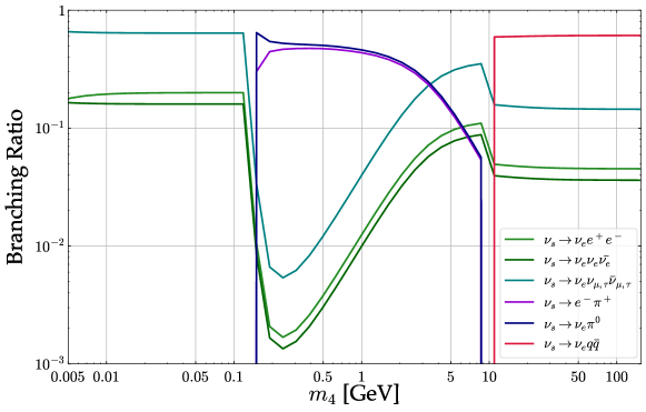
Figure 4: Branching ratio of heavy neutrino as a function of its mass (which is independent of the mixing parameter $|U_{a4}|^{2}$). We show several leading decay channels for clarity. We assume the heavy neutrino to be Majorana and for each decay channel the charge-conjugation (if exist) is already included.

3.1 Charged-pion injection

Hadronic injection is well known to have the strongest effect on BBN. In particular, charged pion injections from heavy neutrino decay can modify the proton-to-neutron ($pn$) ratio via strong interaction, the latter being an important parameter set by weak interactions in the standard BBN. Because the charged pions lifetime is much shorter than duration of BBN, we will only need the instantaneous charged pion injection rate from heavy neutrino decay. In other words, the charged pions that cause $pn$ conversion at time $t$ during BBN are from the decay of heavy neutrino at almost the same time $t$.

3.1.1 $\pi^{\pm}$ energy spectrum

For heavy neutrino mass below a few GeV scale, we can use the two-body partial decay rate Eq. (3.4) for the charged pion injection rate,

$$\mathcal{R}_{\nu_{4}\to\pi^{\pm}}(t)=n_{\nu_{4}}(t)\Gamma_{\nu_{4}\to\ell_{a}^{\mp}\pi^{\pm}}\ .$$ (3.6)

The factor $n_{\nu_{4}}$ is obtained using Eq. (3.1). The produced charged pions typically slow down and thermalize in the early universe plasma, before decaying or triggering the $pn$ conversion [56]. As a result, we only need to find out the overall number of pions instead of their energy spectrum.

For $\nu_{4}$ much heavier than GeV scale, the decay into pions first occurs at quark level. We use Pythia 8.2 [57] to simulate the hadronization of the heavy neutrino decay products. The resulting number of charged pions per $\nu_{4}$ (we call this quantity $N_{\nu_{4}\to\pi^{\pm}}$) is shown in the left panel of Fig. 5 as a function of $m_{4}$. The corresponding charged pion injection rate is

$$\mathcal{R}_{\nu_{4}\to\pi^{\pm}}=n_{\nu_{4}}(t)\Gamma_{\rm tot}N_{\nu_{4}\to\pi^{\pm}}\ .$$ (3.7)

We will not consider $pn$ conversion triggered by neutral pions because they decay at much shorter lifetime. The effects of photons resulting from $\pi^{0}$ will be addressed later on.

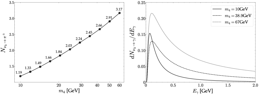
Figure 5: Left panel: Multiplicity of charged pions per each heavy neutrino decay as a function of its mass $m_{4}$. Right panel: Photon energy spectrum (differential multiplicity) from heavy neutrino decay. These results apply when the heavy neutrino mass is above $\sim 10$ GeV and are simulated using Pythia 8.2.

3.1.2 Proton-neutron conversion with $\pi^{\pm}$

The most important effects of heavy neutrino decay in our analysis are the proton-neutron conversion induced by charged pions. The Boltzmann equation for proton and neutron processes are

$$\begin{split}\frac{dn_{p}}{dt}\simeq\left(\dfrac{dn_{p}}{dt}\right)_{\rm SBBN}&+\mathcal{R}_{\nu_{4}\to\pi^{+}}(t)\times\frac{n_{n}(t)\langle\sigma v\rangle_{\pi^{+}n\to p\pi^{0}}}{\Gamma_{\pi^{+}}+n_{n}(t)\langle\sigma v\rangle_{\pi^{+}n\to p\pi^{0}}}\\ &-\mathcal{R}_{\nu_{4}\to\pi^{-}}(t)\times\frac{n_{p}(t)\left(\langle\sigma v\rangle_{\pi^{-}p\to n\gamma}+\langle\sigma v\rangle_{\pi^{-}p\to n\pi^{0}}\rule{0.0pt}{11.38109pt}\right)}{\Gamma_{\pi^{-}}+n_{p}(t)\left(\langle\sigma v\rangle_{\pi^{-}p\to n\gamma}+\langle\sigma v\rangle_{\pi^{-}p\to n\pi^{0}}\rule{0.0pt}{11.38109pt}\right)}\ ,\\ \frac{dn_{n}}{dt}=\left(\frac{dn_{n}}{dt}\right)_{\rm SBBN}&-\mathcal{R}_{\nu_{4}\to\pi^{+}}(t)\times\frac{n_{n}(t)\langle\sigma v\rangle_{\pi^{+}n\to p\pi^{0}}}{\Gamma_{\pi^{+}}+n_{n}(t)\langle\sigma v\rangle_{\pi^{+}n\to p\pi^{0}}}\\ &+\mathcal{R}_{\nu_{4}\to\pi^{-}}(t)\times\frac{n_{p}(t)\left(\langle\sigma v\rangle_{\pi^{-}p\to n\gamma}+\langle\sigma v\rangle_{\pi^{-}p\to n\pi^{0}}\rule{0.0pt}{11.38109pt}\right)}{\Gamma_{\pi^{-}}+n_{p}(t)\left(\langle\sigma v\rangle_{\pi^{-}p\to n\gamma}+\langle\sigma v\rangle_{\pi^{-}p\to n\pi^{0}}\rule{0.0pt}{11.38109pt}\right)}\ .\end{split}$$ (3.8)

On the right-hand side of both equations, the first term denotes all the processes in the standard BBN (SBBN). The new effects due to heavy neutrino to charged pion decay are encoded by the second and third terms. The rates $\mathcal{R}_{\nu_{4}\to\pi^{\pm}}(t)$ is defined in Eqs. (3.6), (3.7).

The fractional factors multiplying with $\mathcal{R}$ show the competition between the pion decay rate and their nuclear reaction with protons and neutrons in the universe. The conversion cross sections for thermalized pions are [56]

$$\langle\sigma v\rangle_{\pi^{-}p\to n\gamma}\simeq 0.57\,\text{mb}\ ,\quad\langle\sigma v\rangle_{\pi^{-}p\to n\pi^{0}}\simeq 0.88\,\text{mb}\ ,\quad\langle\sigma v\rangle_{\pi^{+}n\to p\pi^{0}}\simeq 1.7\,\text{mb}\ .$$ (3.9)

The charged pion decay rate is $\Gamma_{\pi^{\pm}}=\left(2.6\times 10^{-8}\,{\rm sec}\right)^{-1}$. We use the SBBN solutions for the proton and neutron number densities, $n_{p,n}(t)$, which acknowledge that new physics is not permitted to cause significant departure from SBBN predictions.

3.2 Photon injection

Electromagnetic injection is another potentially important effect of new physics on BBN. The photons could potentially be absorbed by the primordial elements and dissociate them into nucleons or lighter nuclei. During the BBN time, photons are tightly coupled to the background thermal plasma through Compton scatterings and the Breit–Wheeler processes with a large optical depth. As a result, the non-thermal photon lifetime is very short. Similar to the approximation made in the charged pion case, for the photon injection rate we only consider the instantaneous decay of the heavy neutrino.

3.2.1 Photon energy spectrum

The photon triggered nucleus dissociation cross sections are energy dependent thus we will need to find out the energy spectrum of photons from heavy neutrino decay. For heavy neutrino mass below a few GeV scale, the cascade process is $\nu_{4}\to\nu_{a}\pi^{0}$, followed by $\pi^{0}\to\gamma\gamma$. In the first step, because the heavy neutrino is already non-relativistic when decaying, the resulting $\pi^{0}$ has approximately fixed energy $E_{\pi}=(m_{4}^{2}+m_{\pi}^{2})/(2m_{4})$. In the boosted-pion reference frame, the resulting photon energy spectrum is

$$\frac{d\mathcal{R}_{\nu_{4}\to\gamma}}{dE_{\gamma}}=n_{\nu_{4}}(t)\Gamma_{\nu_{4}\to\nu_{a}\pi^{0}}\frac{2}{E_{\pi}\beta_{\pi}}\Theta\left(E_{\gamma}-(E_{\gamma})_{\rm min}\rule{0.0pt}{11.38109pt}\right)\Theta\left((E_{\gamma})_{\rm max}-E_{\gamma}\rule{0.0pt}{11.38109pt}\right)\ ,$$ (3.10)

where $\beta_{\pi}=(m_{4}^{2}-m_{\pi}^{2})/(m_{4}^{2}+m_{\pi}^{2})$, $\Theta$ is the unit-step function, and we observe that the photons have a flat energy distribution in the boosted frame of decaying $\pi^{0}$, with

$$(E_{\gamma})^{\rm max}_{\rm min}=\frac{E_{\pi}}{2}(1\pm\beta_{\pi})\ .$$ (3.11)

On the other hand, for $\nu_{4}$ much heavier than GeV scale, we run Pythia to obtain the resulting photon spectrum from heavy neutrino decay. The injected photon energy spectrum in this case is

$$\frac{d\mathcal{R}_{\nu_{4}\to\gamma}}{dE_{\gamma}}=n_{\nu_{4}}(t)\Gamma_{\rm tot}\frac{dN_{\nu_{4}\to\gamma}}{dE_{\gamma}}\ ,$$ (3.12)

where $N_{\nu_{4}\to\gamma}$ is the number of photons per heavy neutrino decay obtained based on pythia simulation. The spectrum $dN_{\nu_{4}\to\gamma}/dE_{\gamma}$ is shown in the right panel of Fig. 5 for several choices of the heavy neutrino mass.

3.2.2 Photodissociation of nuclei

Here, we present the set of Boltzmann equations that include the non-thermal photodissociation effects. For simplicity of discussion, we only add new terms related to deuterium destruction. Our numerical analysis goes beyond this and includes nine light nuclei dissociation channels up to helium-4 [58]. The corresponding cross sections are listed in the appendix B.

The deuterium dissociation process is $d+\gamma\to p+n$, which is inverse to the first step of fusion processes of BBN. It depletes deuterium in the universe and contributes to the populations of proton and neutron. In this case, the modified Boltzmann equations are

$$\begin{split}\frac{dn_{d}}{dt}&=\left(\frac{dn_{d}}{dt}\right)_{\rm SBBN}-\int_{Q}^{\infty}dE_{\gamma}\frac{d\mathcal{R}_{\nu_{4}\to\gamma}}{dE_{\gamma}}\frac{n_{d}\langle\sigma v\rangle_{d\gamma\to np}}{\Gamma^{\gamma}_{\rm tot}}+\cdots\ ,\\ \frac{dn_{p,n}}{dt}&=\left(\frac{dn_{p,n}}{dt}\right)_{\rm SBBN}+\int_{Q}^{\infty}dE_{\gamma}\frac{d\mathcal{R}_{\nu_{4}\to\gamma}}{dE_{\gamma}}\frac{n_{d}\langle\sigma v\rangle_{d\gamma\to np}}{\Gamma^{\gamma}_{\rm tot}}+\cdots\ ,\end{split}$$ (3.13)

where the non-thermal photon energy spectrum $d\mathcal{R}_{\nu_{4}\to\gamma}/dE_{\gamma}$ is given above in Eqs. (3.10) or (3.12), and

$$\Gamma^{\gamma}_{\rm tot}=n_{d}(\sigma v)_{d\gamma\to np}+n_{\gamma}(\sigma v)_{\gamma\gamma\to e^{+}e^{-}}+n_{e}(\sigma v)_{e^{\pm}\gamma\to e^{\pm}\gamma}+\cdots\ .$$ (3.14)

On the right-hand side, the deuterium dissociation cross section is

$$\sigma_{d\gamma\to np}(E_{\gamma})=18.75\textrm{mb}\left[\left(\frac{\left|Q\right|(E_{\gamma}-\left|Q\right|)}{E_{\gamma}}\right)^{3}+0.007947\left(\frac{\left|Q\right|(E_{\gamma}-\left|Q\right|)}{E_{\gamma}}\right)^{2}\frac{\left(\sqrt{\left|Q\right|}-\sqrt{0.037}\right)^{2}}{E_{\gamma}-(\left|Q\right|-0.037)}\right]\ ,$$ (3.15)

where $Q=2.2\,$MeV is the deuterium binding energy, and we use the standard BBN values for $n_{d}$, $n_{\gamma}$, $n_{e}$ to evaluate the non-thermal photon reaction rates. $\gamma\gamma\to e^{+}e^{-}$ and $e^{\pm}\gamma\to e^{\pm}\gamma$ stand for the regular QED processes where the energetic photon from heavy neutrino decay scatters with a background electron (Compton scattering [59]) and photon (Breit–Wheeler scattering [60]) from the thermal plasma, respectively. The dots in Eqs. (3.13) and (3.14) represents other nuclei photodissociation rates taken into account by our analysis.

3.3 Neutrino injection

We also consider active neutrinos from the heavy neutral lepton decay. Like charged pions, neutrinos can also cause the $pn$ conversion. Due to the weakly interacting nature, the conversion effect from neutrinos is weaker than pions if both are present from the decay of heavy neutrino. However, if the heavy neutrino mass lies below the pion decay threshold, it can only decay into light neutrinos and $e^{\pm}$. This is the mass region where neutrinos could play a leading role in modifying BBN predictions.

3.3.1 Neutrino energy spectrum

Different from charged pions and photons, neutrino does not decay and interacts feebly. This leads to an accumulation effect in the number of neutrinos. At any given time, the neutrinos participating in the $pn$ conversion could be produced from heavy neutrino decays in the past, roughly, one mean free path back in time.

We following the general approach described in [61] to derive the phase space distribution function of active neutrinos from heavy neutrino decay,

$$f_{\nu_{e}}(x,T)=\frac{2\pi^{2}}{x^{2}}\int_{T}^{T_{\rm max}(x)}\frac{dT^{\prime}}{T^{\prime}}\frac{n_{\nu_{4}}(T^{\prime})}{m_{4}H(T^{\prime})T^{\prime 2}}\sum_{i}\Gamma_{\nu_{4}\to\nu}^{i}g_{i}\left(\frac{T^{\prime}}{m_{4}}x\right)\ ,$$ (3.16)

where $x=E_{\nu}/T$, the sum over $i$ goes over the leptonic decay channels in Eq. (3.3) that can produce $\nu_{e}$ in the final state. $\Gamma_{\nu_{4}\to\nu}^{i}$ is the partial decay rate for one of the decay modes there, and $g_{i}$ is corresponding dimensionless neutrino spectral function per heavy neutrino decay,

$$g_{i}(\omega)=\frac{n}{\Gamma_{\nu_{4}\to\nu}^{i}}\frac{d\Gamma_{\nu_{4}\to\nu}^{i}}{d\omega}\ ,\quad\int d\omega g(\omega)=n\ ,$$ (3.17)

where $\omega=E_{\nu}/m_{4}$ and $n$ is the number of $\nu_{e}$ produced in the decay mode. For the $\nu_{4}\to\nu_{a}\nu_{a}\bar{\nu}_{a}$ decay channel, $n=2$. For the other channels $n=1$. For weak-boson mediated decay modes in Eq. (3.3), the $g_{i}$ functions take a universal form,

$$g_{i}(\omega)=16n\omega^{2}(3-4\omega)\ .$$ (3.18)

The temperature upper limit $T_{\rm max}$ of the integral of Eq. (3.16) is

$$T_{\rm max}(x)\simeq\frac{1.3}{\left(G_{F}^{2}M_{\rm P}x\rule{0.0pt}{8.53581pt}\right)^{1/3}}\ .$$ (3.19)

It is set by $\Gamma_{a}=H$ where $\Gamma_{a}$ is the reaction rate of an active neutrino with energy $E_{\nu}=xT$. This upper limit ensures that the neutrinos produced from $\nu_{4}$ decay will free stream, except for occasionally striking on the remaining nucleon in the universe to trigger the $pn$ conversion.

The heavy neutrino considered in this work experiences no CP violation in its tree-level production and decay. As a result, the resulting neutrino and anti-neutrino distributions are identical

$$f_{\bar{\nu}_{e}}=f_{\nu_{e}}\ .$$ (3.20)

3.3.2 Proton-neutron conversion with $\nu_{e}$

Like charged pions, neutrino injection can also trigger the $pn$ conversion via weak interactions. Due to the large mass of muon and tau leptons, we focus on the $\nu_{e}$ neutrinos for the $pn$ conversion process. With the neutrino PSD function derived in Eq. (3.16), the Boltzmann equations for proton and neutron are as follows

$$\begin{split}\dfrac{dn_{p}}{dt}&=\left(\dfrac{dn_{p}}{dt}\right)_{\rm SBBN}-n_{p}\int\dfrac{d^{3}p_{\bar{\nu}_{e}}}{(2\pi)^{3}}f_{\bar{\nu}_{e}}\sigma_{p\bar{\nu}\to ne^{+}}+n_{n}\int\dfrac{d^{3}p_{\nu_{e}}}{(2\pi)^{3}}f_{\nu_{e}}\sigma_{n\nu\to pe^{-}}\ ,\\ \dfrac{dn_{n}}{dt}&=\left(\dfrac{dn_{n}}{dt}\right)_{\rm SBBN}+n_{p}\int\dfrac{d^{3}p_{\bar{\nu}_{e}}}{(2\pi)^{3}}f_{\bar{\nu}_{e}}\sigma_{p\bar{\nu}\to ne^{+}}-n_{n}\int\dfrac{d^{3}p_{\nu_{e}}}{(2\pi)^{3}}f_{\nu_{e}}\sigma_{n\nu\to pe^{-}}\ .\end{split}$$ (3.21)

With the assumption of $E_{\nu}\gg m_{e}$ and $m_{n}\simeq m_{p}\equiv m_{N}$, the nucleon-conversion cross section take the approximate form (in the rest frame of the initial-state nucleon)

$$(\sigma v)_{p\bar{\nu}_{e}\to ne^{+}} \simeq\frac{4G_{F}^{2}E_{\nu}^{2}m_{N}\left[16(g_{A}^{2}-g_{A}+1)E_{\nu}^{2}+12(2g_{A}^{2}-g_{A}+1)m_{N}E_{\nu}+3(3g_{A}^{2}+1)m_{N}^{2}\right]}{3\pi(m_{N}+2E_{\nu})^{3}}\ ,$$ (3.22)

$$(\sigma v)_{n\nu_{e}\to pe^{-}} \simeq\frac{4G_{F}^{2}E_{\nu}^{2}m_{N}\left[16(g_{A}^{2}+g_{A}+1)E_{\nu}^{2}+12(2g_{A}^{2}+g_{A}+1)m_{N}E_{\nu}+3(3g_{A}^{2}+1)m_{N}^{2}\right]}{3\pi(m_{N}+2E_{\nu})^{3}}\ ,$$

where $g_{A}=1.27$ is the nucleon axial-vector current coupling constant. In our numerical simulation, we keep the electron mass and the proton-neutron mass difference, which set the neutrino energy threshold for the $p\bar{\nu}_{e}\to ne^{+}$ reaction to occur,

$$(E_{\nu})_{\rm min}\simeq\frac{(m_{n}-m_{p})^{2}-m_{e}^{2}}{2(m_{n}-m_{p})}\ .$$ (3.23)

As a useful remark on the details, even in the case where the heavy neutrino only mixes with $\nu_{\mu}$ or $\nu_{\tau}$ and it is lighter than the corresponding charged lepton, weak interaction still allows it decay into $\nu_{e}$ via the $Z$-boson exchange.

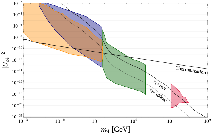
Figure 6: Anatomy of BBN constraints on the heavy neutrino mass versus mixing parameter space, with the shaded regions excluded due to various effects during BBN. Orange region is for temporary matter domination. In the blue, green and red regions, the heavy neutrino have different dominant decay modes and its decay products affect the primordial element production in different ways, detailed in the text. The black curves correspond to the thermalization boundary (see also Fig. 2), and the heavy neutrino lifetime equals 1 (solid) second and 100 seconds (dashed).

4 Results

Fig. 6 show the main result of this analysis for heavy neutrino mixing with $\nu_{e}$. It further divides the BBN exclusion in Fig. 1 into various colored regions where the heavy neutrino itself or its decay products impact the BBN prediction in different ways.

First, the effect of temporary matter domination before the decay of heavy neutrino described in Sec. 2.3 excludes the orange shaded region in the upper-left part of the figure, with the thermalization line penetrating through. Above this line, the heavy neutrino was once in thermal equilibrium. As discussed in sec. 2.1, the heavy neutrino always decouples relativistically. With a lifetime longer than $\sim 1$ second (corresponding to the upper boundary of the orange region), its energy density can come into domination over that of radiation during BBN. For heavy neutrino mass below a few MeV scale, the orange shaded region shrinks and points to larger values of $|U_{e4}|^{2}$ above the thermalization line. In this low mass range, a smaller $|U_{e4}|^{2}$ leads to too early decoupling, before the QCD phase transition, and in turn a less populous heavy neutrinos (a $g_{*S}$ effect).

For the orange shaded region below the thermalization line, the heavy neutrino never reaches thermal equilibrium with the Standard Model plasma and its abundance is built up by the freeze in mechanism described sec. 2.2. In this region, the population of heavy neutrino is proportional to $|U_{e4}|^{2}$. Below the lower boundary of the orange shaded region, the freeze-in production of heavy neutrino is not efficient.

It is worth noting that the orange shaded region disappears for heavy neutrino mass above $\sim 140$ MeV. In this mass range, the heavy neutrino to pion decay channel opens up which is a two-body decay. Comparing the decay coefficients in Eqs. (3.3) and (3.4), this gives a boost factor of $\sim(10^{2}-10^{3})$ in the $\nu_{4}$’s total decay rate. For the lifetime to remain comparable or longer than 1 second, a much smaller mixing parameter $|U_{e4}|^{2}$ is required. This effect also manifests as the down turn of the $\tau_{4}=1$ second curve when $m_{4}$ goes above the pion mass threshold. As a result, the orange shaded region quickly shrinks to below the thermalization line where the freeze-in production is too low and temporary matter domination does not occur.

Next, we move on to discuss the effects of heavy neutrino decay on the primordial element abundances. We focus on deuterium and helium, which are the most produced nuclei from BBN and their abundances are the most precisely measured [62]

$$\left.\text{D}/\text{H}\right|_{\text{p}} =(25.47\pm 0.25)\times 10^{-6}\ ,$$ (4.1)

$$\text{Y}_{\text{p}} =0.245\pm 0.003\ .$$

To simulate predictions of the heavy neutrino model, we use the public code PRyMordial [63] which is built with a complete network of nuclear reactions in SBBN and the portal to incorporate new physics effects. In addition to the model parameters $m_{4}$ and $|U_{\alpha 4}|^{2},(\alpha=e,\mu,\tau)$, there are two cosmological parameters with non-negligible uncertainties, the baryon asymmetry $\eta_{b}$ and neutron lifetime $\tau_{n}$,

$$\eta_{b} =6.1\times 10^{-10}\pm 5.5\times 10^{-12}\ ,$$ (4.2)

$$\tau_{n} =878.4\pm 0.5\,\text{sec}\ .$$

It is useful to note that the uncertainties in $\eta_{b}$ and $\tau_{n}$ propagate to the model predictions of $\left.\text{D}/\text{H}\right|_{\text{p}}$ and $\text{Y}_{\text{p}}$. The theory prediction error bars are comparable to those from experimental observations [64]. We include both to derive the BBN exclusion regions.

The decay of heavy neutrino during BBN excludes the blue, green, and yellow shaded regions in Fig. 6 at 99% confidence level. All these exclusion regions lie below the $\tau_{4}\simeq 0.1$ second curve, consistent with the lifetime upper limit found in previous analyses [49, 50]. It is worth emphasizing that this is not the absolute upper limit on the lifetime of heavy neutrino. As pointed out in the introduction, in the minimal model the BBN constraint will not apply for very long lifetime, or very small $|U_{e4}|^{2}$, leading to the lower boundary of the exclusion region. See also Fig. 8 in below.

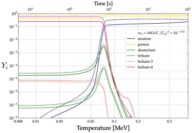
Figure 7: Temperature evolution of primordial element abundance. Time goes from right to left. Solid lines are for the standard cosmology, and dashed lines are the results in the presence of a heavy neutrino that decays during BBN.

In the yellow shaded region in Fig. 6, with $m_{4}$ lying well above $\sim$ 10 GeV, the exclusion only applies to very small $|U_{e4}|^{2}$ where the heavy neutrino experiences freeze-in production in the early universe. As explained in sections 3.1.1 and 3.2.1, we run Pythia to obtain the energy spectrum of pions and photons from the heavy neutrino decay. We focus on $m_{4}>10$ GeV for perturbative QCD and the Pythia results to be valid. In this region, the $pn$ conversion triggered by charged pions plays a by-far dominant role in shifting the abundances of $\left.\text{D}/\text{H}\right|_{\text{p}}$ and $\text{Y}_{\text{p}}$ from the SBBN predictions. Fig. 7 shows the temperature (time) evolution of primordial element abundances during BBN. Solid curves are for SBBN whereas dashed curves are for BBN with a decaying heavy neutrino $\nu_{4}$. The arrow of time points from right to left. The model parameters are chosen to be $m_{4}=10\,$GeV and $|U_{e4}|^{2}=10^{-17.9}$, this correspond to a heavy neutrino lifetime $\tau_{4}=9.58$ sec. Throughout the decay of $\nu_{4}$, the charged pions in the decay product can increase the neutron population in the universe. It is interesting to note that if the decay is active near the weak interaction decoupling (around $T=0.8\,$MeV), it can alter the thermal $pn$ ratio, the initial condition for BBN, because the $pn$ conversion considered here is a non-thermal effect. As a result of the higher neutron population, the so-called "deuterium-bottleneck" is widened, i.e., deuterium formation is the first step of the nucleosynthesis chain. With more deuteriums, the abundance of other elements (deuterium, tritium and helium-4) are also enhanced accordingly. The cost for all these increases is a deficit of the proton abundance as yellow curve indicates.

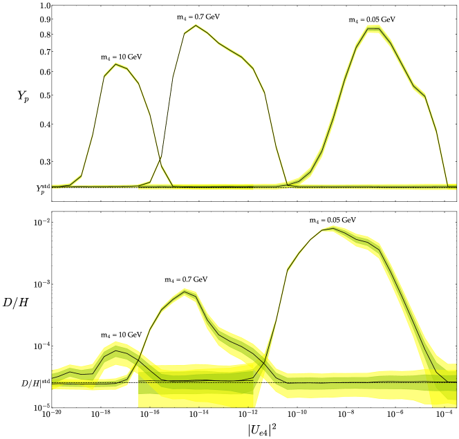
Figure 8: BBN prediction of final helium-4 (top panel) and deuterium bottom panel abundances as function of $|U_{e4}|^{2}$, for three choices of heavy neutrino mass $m_{4}$. In both plots, the green and regions show the 1 and $2\sigma$ theoretical uncertainty (due to uncertainties in $\eta_{b}$ and $\tau_{n}$, see Eq. (4.2)). The central values of experimentally measured abundances are shown by black dashed lines. On each curve, there is a range of $|U_{e4}|^{2}$ where excessive helium-4 and deuterium are produced and is thus ruled out.

Similarly, the green shaded region in Fig. 6, with an intermediate $m_{4}$ between the pion mass threshold and a few GeV scale, is excluded primarily by the charged-pion-triggered $pn$ conversion. In this window, we simulate pion production using the two-body decays $\nu_{4}\to\ell_{\alpha}^{\pm}\pi^{\mp}$. The gap of $m_{4}$ between a few and 10 GeV is not shaded due to the complexity of QCD, where one cannot reliably calculate the hadronic decays of heavy neutrino using the quark or meson descriptions. By interpolation, we think this region is likely to be excluded as well.

The partial decay into neutral pions (and promptly into photons) can induce photodissociation of nuclei formed throughout BBN. We include this effect in the Boltzmann equations for nuclei, for both $\nu_{4}$ mass windows discussed above.  Numerically, we find that photodissociation is always subdominant to $pn$ conversion, and its effects alone on $\left.\text{D}/\text{H}\right|_{\text{p}}$ and $\text{Y}_{\text{p}}$ is almost negligible. This can be explained because photodissociation destroys nuclei only after they are formed, after $T\lesssim 100\,$keV or $t\gtrsim 100\,$second, which corresponds to the region below the dashed curve in Fig. 6. Meanwhile, energetic photons from $\pi^{0}$ decay requires $\nu_{4}$ to be heavier than the pion threshold. The union of the two conditions points to a parameter space below the thermalization line, i.e., the heavy neutrino is freeze-in produced and the population is sub-thermal. As a result, we never get sufficient photon injection at the right time for photodissociation to play an important role. Such an argument holds even better for mixing with other neutrino flavors ($\nu_{\mu},\nu_{\tau}$) where the pion decay threshold is pushed higher. This interplay leads us to conclude photodissociation during BBN effect is always a negligible effect for heavy neutrino in the minimal model considered here.

In the blue shaded region of Fig. 6, the $\nu_{4}$ mass lies below the pion threshold and can undergo a three-body leptonic decay into neutrinos and/or $e^{\pm}$. The neutrinos in the final state can also trigger $pn$ conversion via weak interaction as discussed in section 3.3.2. Due to the weakly interacting nature, neutrinos can free stream and build up their phase space distribution until participating the conversion process at a later time. We find the lower part of the blue shaded region overlaps with the exclusion due to temporary matter domination (orange) as discussed earlier, whereas the neutrino triggered $pn$ conversion effect can cover a larger $|U_{e4}|^{2}$ region with $\tau_{4}\gtrsim 0.1\,$sec.

The effects of heavy neutrino decay discussed above are also depicted in Fig. 8 where we hold $m_{4}$ fixed at three values (10 GeV, 0.7 GeV and 0.05 GeV) and vary the active-sterile neutrino mixing $|U_{e4}|^{2}$. The brazilian bands around the solid curves show the theoretical uncertainties in the predictions of $\left.\text{D}/\text{H}\right|_{\text{p}}$ and $\text{Y}_{\text{p}}$, due to uncertainties of cosmological parameters in Eq. (4.2). The horizontal dashed lines show the central values of experimental measurement in Eq. (4.1). For each $\nu_{4}$ mass, there exists a window of $|U_{e4}|^{2}$ values, where both $\left.\text{D}/\text{H}\right|_{\text{p}}$ and $\text{Y}_{\text{p}}$ values are higher than the predictions of SBBN. For higher $m_{4}$, the excluded $|U_{e4}|^{2}$ window shifts to smaller values. The peak of each curve corresponds to $\nu_{4}$ lifetime equals several seconds. The far-left side of the peaks are not excluded because the heavy neutrino is not efficiently produced by the freeze-in mechanism, whereas the far-right side of the peaks are not excluded because the heavy neutrino decays away before BBN.

Finally, we also consider heavy neutrino mixing with $\nu_{\mu}$ or $\nu_{\tau}$ flavors. The results are shown in Fig. 9. The physics involved in BBN is similar, except for the modification of mass windows due to non-negligible muon and tau lepton masses. Compared to previous works, our results present the entire BBN excluded region and a panoramic view over the heavy neutrino parameter space.

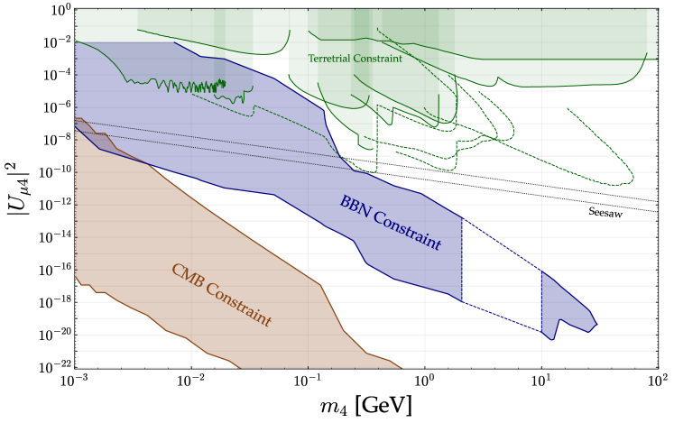
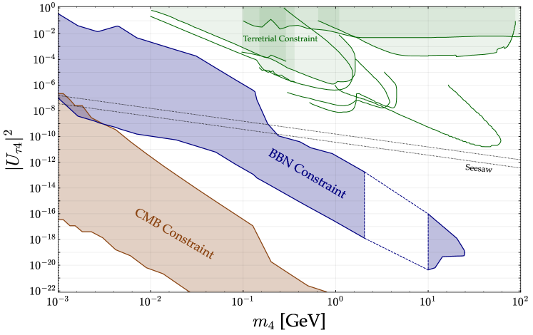
Figure 9: Similar to Fig:1 but for heavy neutrino mixing with $\nu_{\mu}$ (top panel) or $\nu_{\tau}$ (bottom panel).

5 CMB Constraint on very Long-lived Heavy Neutrino

For heavy neutrino with lifetime much longer than the BBN timescale, we consider another useful constraint on the energy injection into the universe during the formation of CMB. We adopt the CMB constraint result set on decaying dark matter previously derived in [65], which puts an lower bound on the lifetime on a particle $X$ assuming it comprises 100% of dark matter in the universe, i.e., $\Omega_{c}h^{2}=0.12$. To translate it for the long-lived heavy neutrino, we note that the population is not tied to $\Omega_{c}$ but determined by the freeze-out or freeze-in mechanisms, as discussed in Section 2. In this case, the lifetime lower limit is set for

$$\tau_{4}>[\tau_{X}]_{\rm min}\times\left[\frac{n_{4}\left(m_{4},|U_{a4}|^{2}\right)}{n_{X}}\right]_{T=0.3\,\rm eV}\ ,$$ (5.1)

where $n_{4}$ is the number density of heavy neutrino $\nu_{4}$ evolved to the time of recombination, where $T\simeq 0.3$ eV, and it includes the exponential decaying factor. $n_{X}\simeq(T/2.7\,{\rm K})^{3}\rho_{c}\Omega_{c}/m_{X}$ is the dark matter number density at the same time and $\rho_{c}=1.05\times 10^{-5}h^{2}\,{\rm GeV/cm^{3}}$ is the critical density of today’s universe. $[\tau_{X}]_{\rm min}$ as a function of $m_{X}$ (set to be equal to $m_{4}$ here) is obtained by digitalizing Fig. 8 of [65] (approximately, $[\tau_{X}]_{\rm min}\simeq 10^{25}\,$s for $m_{X}$ above MeV scale). The limit from Eq. (5.1) translates into the lower boundary of the brown shaded region in Figs. 1 and 9. Near this lower boundary, the heavy neutrino has a lifetime longer than the age of the universe [66] and it can be part of the dark matter in the universe. As a useful comparison, the CMB constraint on $|U_{a4}|^{2}$ is stronger than the indirect detection limit on $\nu_{4}\to\nu\gamma$ decay found in [67].

Similar to the argument made for BBN, the CMB constraint does not apply for sufficiently large $|U_{a4}|^{2}$ where the heavy neutrino decay happens too early. Without detailed analysis, we simply set this upper boundary as where the heavy neutrino lifetime is equal to the age of universe when $T\simeq 10\,$eV, which corresponds to the onset of large scale structure formation [68]. There is a gap of allowed parameter space between the BBN and CMB exclusion regions.

6 Conclusion

In this work, we explore the BBN constraints on a heavy neutrino in the minimal model. The heavy neutrino is introduced as a pure gauge singlet fermion and it could interact with other known particles only through mixing with active neutrinos after the electroweak symmetry breaking. Such a setup is found in beyond the Standard Model theories of the type-I seesaw mechanism for neutrino mass generation, or neutrino portal dark sectors. When the mixing occurs with a single active neutrino flavor $\nu_{\alpha},\ (\alpha=e,\mu,\tau)$, the minimal has only two new parameters, the heavy neutrino mass $m_{4}$ and the mixing $|U_{a4}|^{2}$, defined in Eq. (1.1). We point out that not only the decays of the heavy neutrino are fully determined by the two parameters, but also its production mechanism in the early universe. For sufficiently large $|U_{a4}|^{2}$, the relic abundance of heavy neutrino (before decaying away) is set by the thermal freeze-out mechanism similar to the decoupling of light neutrinos. For smaller $|U_{a4}|^{2}$, the production takes place via active-sterile neutrino oscillation in the early universe plasma (a kind of freeze-in mechanism). For each point in the $m_{4}$ versus $|U_{a4}|^{2}$ parameter space, we calculate the heavy neutrino’s abundance using either of the above production mechanism and feed the result as the input for our BBN analysis. It is useful to point out that the time scales for the heavy neutrino production and decay of heavy neutrino are always well separated.

For the BBN constraints, we consider the effects of temporary matter domination prior to the decay of heavy neutrino, as well as non-thermal energy injections due to the decay. In the latter case, we find that hadronic energy injection in the form of $\pi^{\pm}$ plays the dominant role in modifying the predicted helium-4 and deuterium abundances, whereas the effect of nuclear photodissociation injection is always negligible. Injection of light neutrinos from the decay is relevant for heavy neutrino mass below the pion threshold. The BBN excluded parameter space extends from MeV to tens of GeV. For large masses, it can be sensitive to a mixing parameter $|U_{a4}|^{2}$ as small as $10^{-20}$. For even smaller mixings, there is no BBN constraint on the heavy neutrino because the heavy neutrino population via the freeze in mechanism is too small. In that region, we sketch a CMB constraint on the very long-lived heavy neutrino using the energy injection argument.

Our analysis gives a complete description of the fate and impact of an unstable heavy neutrino in the early universe. Its production and decay are both determined by the two minimal model parameters, with little room for assumptions. For the freeze-in production mechanism, we assume zero initial abundance of the heavy neutrino. This assumption could be relaxed with additional new physics at high scale, but they would result in an enhanced heavy neutrino abundance and stronger BBN and CMB constraints. In contrast, the freeze-out mechanism is not sensitive to high scale physics and the BBN constraint in that region of parameter space is robust.

Our main results, Figs. 1 and 9, show that BBN excludes the low-scale type-I seesaw mechanism with heavy neutrino mass below a few hundred MeV. This conclusion holds even in the presence of the caveat for large $|U_{a4}|^{2}$ noticed in [69, 70]. For higher masses, BBN and CMB can probe more weakly-coupled heavy neutrinos and complements terrestrial probes with the energy and intensity frontier experiments.

Appendix A Boltzmann equation for active-sterile neutrino oscillation

To describe the collisional oscillation for dark matter production, we consider the phase-space density matrix in the $(\nu_{a},\nu_{s})$ space

$$\mathcal{F}=\begin{pmatrix}f_{a}&f_{as}\\ f_{sa}&f_{s}\end{pmatrix}\ ,$$ (A.1)

where the diagonal elements $f_{a}(f_{s})$ stand for phase space distributions for the active (sterile) neutrino. Quantum effects lie in the off-diagonal elements.

The density matrix evolves according to the quantum kinetic equations [53, 71, 72],

$$\begin{split}H\frac{\partial f_{a}}{\partial\log a}&=\frac{i}{2}\Delta\sin(2\theta)\left(f_{as}-f_{sa}\rule{0.0pt}{11.38109pt}\right)+\Gamma_{A}\left(f_{a}-f_{\rm eq}\rule{0.0pt}{11.38109pt}\right)\ ,\\ H\frac{\partial f_{as}}{\partial\log a}&=\frac{i}{2}\left[\Delta\sin(2\theta)\left(f_{a}-f_{s}\rule{0.0pt}{11.38109pt}\right)+2\left(\Delta\cos(2\theta)-V\rule{0.0pt}{11.38109pt}\right)f_{as}\rule{0.0pt}{17.07164pt}\right]-\frac{\Gamma}{2}f_{as}\ ,\\ H\frac{\partial f_{sa}}{\partial\log a}&=-\frac{i}{2}\left[\Delta\sin(2\theta)\left(f_{a}-f_{s}\rule{0.0pt}{11.38109pt}\right)+2\left(\Delta\cos(2\theta)-V\rule{0.0pt}{11.38109pt}\right)f_{sa}\rule{0.0pt}{17.07164pt}\right]-\frac{\Gamma}{2}f_{sa}\ ,\\ H\frac{\partial f_{s}}{\partial\log a}&=-\frac{i}{2}\Delta\sin(2\theta)\left(f_{as}-f_{sa}\rule{0.0pt}{11.38109pt}\right)\ .\\ \end{split}$$ (A.2)

In the first equation, $\Gamma_{A}$ is relevant for the active neutrino’s chemical potential and equals to their total annihilation/co-annihilation rate. On the other hand, $\Gamma$ in the second and third equation is relevant for the decoherence of the neutrino state and receives contribution from both annihilation and scattering rates. It is given by Eq. (2.6) and (2.7). $\Gamma$ must come with a prefactor $1/2$ because it multiplies with the off-diagonal elements of the density matrix (wavefunction is the “square root” of density matrix). All the other quantities involved in this equation are also defined below Eq. (2.1).

To proceed, we consider early universe where the temperature is much higher than MeV and the weak interaction rates $\Gamma,\Gamma_{A}$ are much higher than the Hubble parameter $H$. This bring about two simplifications to the set of equation in Eq. (A.2). First, $\Gamma_{A}\gg H$ locks $f_{a}$ for active neutrinos to the thermal distribution

$$f_{a}=f_{\rm eq}\ .$$ (A.3)

With this, the second equation of Eq. (A.2) can be written as

$$\frac{\partial f_{as}}{\partial\log a}=\left[\frac{i}{H}\left(\Delta\cos(2\theta)-V\rule{0.0pt}{11.38109pt}\right)-\frac{\Gamma}{2H}\rule{0.0pt}{17.07164pt}\right]f_{as}+\frac{i}{2H}\Delta\sin(2\theta)\left(f_{\rm eq}-f_{s}\rule{0.0pt}{11.38109pt}\right)\ .$$ (A.4)

For clarify, we define $\tau=\log a$,

$$\begin{split}g(\tau)&\equiv\frac{i}{H}\left(\Delta\cos(2\theta)-V\rule{0.0pt}{11.38109pt}\right)-\frac{\Gamma}{2H}\ ,\\ h(\tau)&\equiv\frac{i}{2H}\Delta\sin(2\theta)\left(f_{\rm eq}-f_{s}\rule{0.0pt}{11.38109pt}\right)\ ,\end{split}$$ (A.5)

and rewrite Eq. (A.4) as

$$\frac{df_{as}}{d\tau}=g(\tau)f_{as}+h(\tau)\ .$$ (A.6)

With initial condition $f_{as}(0)=0$, the solution to the non-homogeneous equation takes the form

$$f_{as}(\tau)=\int_{0}^{\tau}d\tau^{\prime}h(\tau^{\prime})\exp\int_{\tau^{\prime}}^{\tau}d\tau^{\prime\prime}g(\tau^{\prime\prime})\ .$$ (A.7)

In the limit $\Gamma\gg H$, we have $\left|{\rm Re}[g(\tau)]\right|\gg 1$ but ${\rm Re}[g(\tau)]<0$. As a result, the $\tau^{\prime}$ integral in the above equation is dominated by contributions with $\tau^{\prime}\lesssim\tau$, otherwise the exponential factor is strongly suppressed. This observation allows us to write

$$f_{as}(\tau)\simeq h(\tau)\int_{0}^{\tau}d\tau^{\prime}\exp\int_{\tau^{\prime}}^{\tau}d\tau^{\prime\prime}g(\tau^{\prime\prime})\simeq\frac{h(\tau)}{g(\tau)}\int_{0}^{\tau}d\tau^{\prime}g(\tau^{\prime})\exp\int_{\tau^{\prime}}^{\tau}d\tau^{\prime\prime}g(\tau^{\prime\prime})\ .$$ (A.8)

Next we introduce

$$G(\tau^{\prime},\tau)\equiv\int_{\tau^{\prime}}^{\tau}d\tau^{\prime\prime}g(\tau^{\prime\prime})\quad\Rightarrow\quad dG(\tau^{\prime},\tau)=-g(\tau^{\prime})d\tau^{\prime}\ ,$$ (A.9)

which allows Eq. (A.8) to be rewritten as

$$\begin{split}f_{as}(\tau)&\simeq-\frac{h(\tau)}{g(\tau)}\int_{0}^{\tau}e^{G(\tau^{\prime},\tau)}dG(\tau^{\prime},\tau)\\ &=-\frac{h(\tau)}{g(\tau)}\exp\left[G(\tau^{\prime},\tau)\right]^{\tau^{\prime}=\tau}_{\tau^{\prime}=0}\\ &=-\frac{h(\tau)}{g(\tau)}\left[1-\exp\int_{0}^{\tau}d\tau^{\prime}g(\tau^{\prime})\right]\\ &\simeq-\frac{h(\tau)}{g(\tau)}\ .\end{split}$$ (A.10)

In the last step, we again used that the factor $-\Gamma/(2H)$ in $g(\tau)$ causes a strong damping to the exponential term allowing it to be dropped.

With the above simplification, we derive

$$f_{as}=f_{sa}^{*}\simeq\frac{i\Delta\sin(2\theta)/2}{\Gamma/2-i(\Delta\cos(2\theta)-V)}\left(f_{\rm eq}-f_{s}\rule{0.0pt}{11.38109pt}\right)\ .$$ (A.11)

Plugging these results into the last equation of Eq. (A.2), we finally obtain

$$\begin{split}\frac{\partial f_{s}}{\partial\log a}&\simeq\frac{\Gamma}{4H}\left[\frac{\Delta^{2}\sin^{2}(2\theta)}{(\Delta\cos(2\theta)-V)^{2}+\Gamma^{2}/4}\right]\left(f_{\rm eq}-f_{s}\rule{0.0pt}{11.38109pt}\right)\ .\end{split}$$ (A.12)

This agrees with the Boltzmann equation Eq. (2.1) in the small $\theta$ limit. In Eq. (2.1), we added a $\Delta^{2}\sin^{2}(2\theta)$ term to the denominator inside the square bracket, which makes it equal to $\sin^{2}(2\theta_{\rm eff})$ defined in Eq. (2.3) and correctly approach to $\sin^{2}(2\theta)$ in the low temperature limit ($\Gamma,V\to 0$).

Appendix B Photodissociation cross sections

In our analysis, we implement the photodissociation processes for elements up to helium-4. The corresponding cross sections are the numerical fits taken from the appendix of [58].

1. $d(\gamma,n)p,\hskip 10.00002ptE_{\gamma,\text{th}}=\left|Q\right|=$2.224\,573\text{\,}\mathrm{MeV}$$
   $\sigma(E_{\gamma})=$18.75\text{\,}\mathrm{mb}$$ $\left[\left(\frac{\sqrt{\left|Q\right|(E_{\gamma}-\left|Q\right|}}{E_{\gamma}}\right)^{3}+0.007947\left(\frac{\sqrt{\left|Q\right|(E_{\gamma}-\left|Q\right|}}{E_{\gamma}}\right)^{2}\frac{\left(\sqrt{\left|Q\right|}-\sqrt{0.037}\right)^{2}}{E_{\gamma}-\left(\left|Q\right|-0.037\right)}\right]$

2. $t(\gamma,n)d,\hskip 10.00002ptE_{\gamma,\text{th}}=\left|Q\right|=$6.257\,248\text{\,}\mathrm{MeV}$$,    $\sigma(E_{\gamma})=$9.8\text{\,}\mathrm{mb}$$ $\frac{\left|Q\right|^{1.95}\left(E_{\gamma}-\left|Q\right|\right)^{1.65}}{E_{\gamma}^{3.6}}$

3. $t(\gamma,np)n,\hskip 10.00002ptE_{\gamma,\text{th}}=\left|Q\right|=$8.481\,821\text{\,}\mathrm{MeV}$$,    $\sigma(E_{\gamma})=$26.0\text{\,}\mathrm{mb}$$ $\frac{\left|Q\right|^{2.6}\left(E_{\gamma}-\left|Q\right|\right)^{2.3}}{E_{\gamma}^{4.9}}$

4. ${}^{3}He(\gamma,p)d,\hskip 10.00002ptE_{\gamma,\text{th}}=\left|Q\right|=$5.493\,485\text{\,}\mathrm{MeV}$$,    $\sigma(E_{\gamma})=$8.88\text{\,}\mathrm{mb}$$ $\frac{\left|Q\right|^{1.75}\left(E_{\gamma}-\left|Q\right|\right)^{1.65}}{E_{\gamma}^{3.4}}$

5. ${}^{3}He(\gamma,np)p,\hskip 10.00002ptE_{\gamma,\text{th}}=\left|Q\right|=$7.718\,058\text{\,}\mathrm{MeV}$$,    $\sigma(E_{\gamma})=$16.7\text{\,}\mathrm{mb}$$ $\frac{\left|Q\right|^{1.95}\left(E_{\gamma}-\left|Q\right|\right)^{2.3}}{E_{\gamma}^{4.25}}$

6. ${}^{4}He(\gamma,p)t,\hskip 10.00002ptE_{\gamma,\text{th}}=\left|Q\right|=$19.813\,852\text{\,}\mathrm{MeV}$$,    $\sigma(E_{\gamma})=$19.5\text{\,}\mathrm{mb}$$ $\frac{\left|Q\right|^{3.5}\left(E_{\gamma}-\left|Q\right|\right)^{1.0}}{E_{\gamma}^{4.5}}$

7. ${}^{4}He(\gamma,n)^{3}He,\hskip 10.00002ptE_{\gamma,\text{th}}=\left|Q\right|=$20.577\,615\text{\,}\mathrm{MeV}$$,    $\sigma(E_{\gamma})=$17.1\text{\,}\mathrm{mb}$$ $\frac{\left|Q\right|^{3.5}\left(E_{\gamma}-\left|Q\right|\right)^{1.0}}{E_{\gamma}^{4.5}}$

8. ${}^{4}He(\gamma,d)d,\hskip 10.00002ptE_{\gamma,\text{th}}=\left|Q\right|=$23.846\,527\text{\,}\mathrm{MeV}$$,    $\sigma(E_{\gamma})=$10.7\text{\,}\mathrm{mb}$$ $\frac{\left|Q\right|^{10.2}\left(E_{\gamma}-\left|Q\right|\right)^{3.4}}{E_{\gamma}^{13.6}}$

9. ${}^{4}He(\gamma,np)d,\hskip 10.00002ptE_{\gamma,\text{th}}=\left|Q\right|=$26.0711\text{\,}\mathrm{MeV}$$,    $\sigma(E_{\gamma})=$21.7\text{\,}\mathrm{mb}$$ $\frac{\left|Q\right|^{4.0}\left(E_{\gamma}-\left|Q\right|\right)^{3.0}}{E_{\gamma}^{7.0}}$

References

- [1] Super-Kamiokande collaboration, Y. Fukuda et al., Evidence for oscillation of atmospheric neutrinos, Phys. Rev. Lett. 81 (1998) 1562–1567, [hep-ex/9807003].
- [2] SNO collaboration, Q. R. Ahmad et al., Measurement of the rate of interactions produced by 8B solar neutrinos at the Sudbury Neutrino Observatory, Phys. Rev. Lett. 87 (2001) 071301, [nucl-ex/0106015].
- [3] SNO collaboration, Q. R. Ahmad et al., Direct evidence for neutrino flavor transformation from neutral current interactions in the Sudbury Neutrino Observatory, Phys. Rev. Lett. 89 (2002) 011301, [nucl-ex/0204008].
- [4] P. Minkowski, at a Rate of One Out of Muon Decays?, Phys. Lett. B 67 (1977) 421–428.
- [5] T. Yanagida, Horizontal gauge symmetry and masses of neutrinos, Conf. Proc. C 7902131 (1979) 95–99.
- [6] S. L. Glashow, The Future of Elementary Particle Physics, NATO Sci. Ser. B 61 (1980) 687.
- [7] R. N. Mohapatra and G. Senjanovic, Neutrino Mass and Spontaneous Parity Nonconservation, Phys. Rev. Lett. 44 (1980) 912.
- [8] M. Gell-Mann, P. Ramond and R. Slansky, Complex Spinors and Unified Theories, Conf. Proc. C 790927 (1979) 315–321, [1306.4669].
- [9] W. H. Furry, On transition probabilities in double beta-disintegration, Phys. Rev. 56 (1939) 1184–1193.
- [10] S. M. Bilenky and C. Giunti, Neutrinoless double-beta decay: A brief review, Mod. Phys. Lett. A 27 (2012) 1230015, [1203.5250].
- [11] J. Engel and J. Menéndez, Status and Future of Nuclear Matrix Elements for Neutrinoless Double-Beta Decay: A Review, Rept. Prog. Phys. 80 (2017) 046301, [1610.06548].
- [12] M. J. Dolinski, A. W. P. Poon and W. Rodejohann, Neutrinoless Double-Beta Decay: Status and Prospects, Ann. Rev. Nucl. Part. Sci. 69 (2019) 219–251, [1902.04097].
- [13] W. Dekens, J. de Vries, K. Fuyuto, E. Mereghetti and G. Zhou, Sterile neutrinos and neutrinoless double beta decay in effective field theory, JHEP 06 (2020) 097, [2002.07182].
- [14] P. D. Bolton, F. F. Deppisch, M. Rai and Z. Zhang, Probing the Nature of Heavy Neutral Leptons in Direct Searches and Neutrinoless Double Beta Decay, 2212.14690.
- [15] R. Friedberg, Experimental Consequences of the Majorana Theory for the Muon Neutrino, Phys. Rev. 129 (1963) 2298–2300.
- [16] C. Y. Chang, G. B. Yodh, R. Ehrlich, R. Plano and A. Zinchenko, Search for Double Beta Decay of K- Meson, Phys. Rev. Lett. 20 (1968) 510–513.
- [17] W.-Y. Keung and G. Senjanovic, Majorana Neutrinos and the Production of the Right-handed Charged Gauge Boson, Phys. Rev. Lett. 50 (1983) 1427.
- [18] A. Atre, T. Han, S. Pascoli and B. Zhang, The Search for Heavy Majorana Neutrinos, JHEP 05 (2009) 030, [0901.3589].
- [19] M. Nemevsek, F. Nesti, G. Senjanovic and Y. Zhang, First Limits on Left-Right Symmetry Scale from LHC Data, Phys. Rev. D 83 (2011) 115014, [1103.1627].
- [20] M. Mitra, G. Senjanovic and F. Vissani, Neutrinoless Double Beta Decay and Heavy Sterile Neutrinos, Nucl. Phys. B 856 (2012) 26–73, [1108.0004].
- [21] M. Drewes, The Phenomenology of Right Handed Neutrinos, Int. J. Mod. Phys. E 22 (2013) 1330019, [1303.6912].
- [22] F. F. Deppisch, P. S. Bhupal Dev and A. Pilaftsis, Neutrinos and Collider Physics, New J. Phys. 17 (2015) 075019, [1502.06541].
- [23] A. de Gouvêa and A. Kobach, Global Constraints on a Heavy Neutrino, Phys. Rev. D 93 (2016) 033005, [1511.00683].
- [24] A. Maiezza, M. Nemevšek and F. Nesti, Lepton Number Violation in Higgs Decay at LHC, Phys. Rev. Lett. 115 (2015) 081802, [1503.06834].
- [25] Y. Cai, T. Han, T. Li and R. Ruiz, Lepton Number Violation: Seesaw Models and Their Collider Tests, Front. in Phys. 6 (2018) 40, [1711.02180].
- [26] M. Nemevšek and Y. Zhang, Dark Matter Dilution Mechanism through the Lens of Large-Scale Structure, Phys. Rev. Lett. 130 (2023) 121002, [2206.11293].
- [27] Y. Zhang, Charged Lepton Flavor Violation at the High-Energy Colliders: Neutrino Mass Relevant Particles, Universe 8 (2022) 164, [2201.00376].
- [28] Q. Bi, J. Guo, J. Liu, Y. Luo and X.-P. Wang, Long-lived Sterile Neutrino Searches at Future Muon Colliders, 2409.17243.
- [29] Z. S. Wang, Y. Zhang and W. Liu, Long-lived sterile neutrinos from an axionlike particle at Belle II, 2410.00491.
- [30] S. Ajmal, P. Azzi, S. Giappichini, M. Klute, O. Panella, M. Presilla et al., Searching for type I seesaw mechanism in a two Heavy Neutral Leptons scenario at FCC-ee, 2410.03615.
- [31] B. Bertoni, S. Ipek, D. McKeen and A. E. Nelson, Constraints and consequences of reducing small scale structure via large dark matter-neutrino interactions, JHEP 04 (2015) 170, [1412.3113].
- [32] J. M. Berryman, A. de Gouvêa, K. J. Kelly and Y. Zhang, Dark Matter and Neutrino Mass from the Smallest Non-Abelian Chiral Dark Sector, Phys. Rev. D 96 (2017) 075010, [1706.02722].
- [33] B. Batell, T. Han, D. McKeen and B. Shams Es Haghi, Thermal Dark Matter Through the Dirac Neutrino Portal, Phys. Rev. D 97 (2018) 075016, [1709.07001].
- [34] N. Orlofsky and Y. Zhang, Neutrino as the dark force, Phys. Rev. D 104 (2021) 075010, [2106.08339].
- [35] Y. Zhang, On dark matter self-interaction via single neutrino exchange potential, Phys. Dark Univ. 44 (2024) 101434, [2310.10743].
- [36] R. V. Wagoner, W. A. Fowler and F. Hoyle, On the Synthesis of elements at very high temperatures, Astrophys. J. 148 (1967) 3–49.
- [37] L. Kawano, Let’s go: Early universe. 2. Primordial nucleosynthesis: The Computer way, .
- [38] P. D. Serpico, S. Esposito, F. Iocco, G. Mangano, G. Miele and O. Pisanti, Nuclear reaction network for primordial nucleosynthesis: A Detailed analysis of rates, uncertainties and light nuclei yields, JCAP 12 (2004) 010, [astro-ph/0408076].
- [39] M. Pospelov, Particle physics catalysis of thermal Big Bang Nucleosynthesis, Phys. Rev. Lett. 98 (2007) 231301, [hep-ph/0605215].
- [40] R. Barbieri and A. Dolgov, Neutrino oscillations in the early universe, Nucl. Phys. B 349 (1991) 743–753.
- [41] K. Kainulainen, Light Singlet Neutrinos and the Primordial Nucleosynthesis, Phys. Lett. B 244 (1990) 191–195.
- [42] K. Enqvist, K. Kainulainen and J. Maalampi, Refraction and Oscillations of Neutrinos in the Early Universe, Nucl. Phys. B 349 (1991) 754–790.
- [43] K. S. Babu and I. Z. Rothstein, Relaxing nucleosynthesis bounds on sterile-neutrinos, Phys. Lett. B 275 (1992) 112–118.
- [44] S. Dodelson and L. M. Widrow, Sterile-neutrinos as dark matter, Phys. Rev. Lett. 72 (1994) 17–20, [hep-ph/9303287].
- [45] D. Gorbunov and M. Shaposhnikov, How to find neutral leptons of the MSM?, JHEP 10 (2007) 015, [0705.1729].
- [46] A. Boyarsky, O. Ruchayskiy and M. Shaposhnikov, The Role of sterile neutrinos in cosmology and astrophysics, Ann. Rev. Nucl. Part. Sci. 59 (2009) 191–214, [0901.0011].
- [47] O. Ruchayskiy and A. Ivashko, Restrictions on the lifetime of sterile neutrinos from primordial nucleosynthesis, JCAP 10 (2012) 014, [1202.2841].
- [48] S. Alekhin et al., A facility to Search for Hidden Particles at the CERN SPS: the SHiP physics case, Rept. Prog. Phys. 79 (2016) 124201, [1504.04855].
- [49] A. Boyarsky, M. Ovchynnikov, O. Ruchayskiy and V. Syvolap, Improved big bang nucleosynthesis constraints on heavy neutral leptons, Phys. Rev. D 104 (2021) 023517, [2008.00749].
- [50] N. Sabti, A. Magalich and A. Filimonova, An Extended Analysis of Heavy Neutral Leptons during Big Bang Nucleosynthesis, JCAP 11 (2020) 056, [2006.07387].
- [51] Planck collaboration, N. Aghanim et al., Planck 2018 results. VI. Cosmological parameters, Astron. Astrophys. 641 (2020) A6, [1807.06209].
- [52] DESI collaboration, A. G. Adame et al., DESI 2024 VI: Cosmological Constraints from the Measurements of Baryon Acoustic Oscillations, 2404.03002.
- [53] G. Sigl and G. Raffelt, General kinetic description of relativistic mixed neutrinos, Nucl. Phys. B 406 (1993) 423–451.
- [54] D. Notzold and G. Raffelt, Neutrino dispersion at finite temperature and density, Nucl. Phys. B 307 (1988) 924–936.
- [55] T.-H. Yeh, K. A. Olive and B. D. Fields, Limits on Non-Relativistic Matter During Big-Bang Nucleosynthesis, 2401.08795.
- [56] M. Pospelov and J. Pradler, Metastable GeV-scale particles as a solution to the cosmological lithium problem, Phys. Rev. D 82 (2010) 103514, [1006.4172].
- [57] T. Sjöstrand, S. Ask, J. R. Christiansen, R. Corke, N. Desai, P. Ilten et al., An introduction to PYTHIA 8.2, Comput. Phys. Commun. 191 (2015) 159–177, [1410.3012].
- [58] R. H. Cyburt, J. R. Ellis, B. D. Fields and K. A. Olive, Updated nucleosynthesis constraints on unstable relic particles, Phys. Rev. D 67 (2003) 103521, [astro-ph/0211258].
- [59] M. E. Peskin and D. V. Schroeder, An Introduction to quantum field theory. Addison-Wesley, Reading, USA, 1995, 10.1201/9780429503559.
- [60] X. Ribeyre, M. Lobet, E. D’Humières, S. Jequier, V. T. Tikhonchuk and O. Jansen, Pair creation in collision of -ray beams produced with high-intensity lasers, Phys. Rev. E 93 (2016) 013201, [1504.07868].
- [61] M. Nemevšek and Y. Zhang, Anatomy of diluted dark matter in the minimal left-right symmetric model, Phys. Rev. D 109 (2024) 056021, [2312.00129].
- [62] Particle Data Group collaboration, R. L. Workman et al., Review of Particle Physics, PTEP 2022 (2022) 083C01.
- [63] A.-K. Burns, T. M. P. Tait and M. Valli, PRyMordial: the first three minutes, within and beyond the standard model, Eur. Phys. J. C 84 (2024) 86, [2307.07061].
- [64] T. Chowdhury and S. Ipek, Neutron lifetime anomaly and Big Bang nucleosynthesis, Can. J. Phys. 102 (2024) 96–99, [2210.12031].
- [65] T. R. Slatyer and C.-L. Wu, General Constraints on Dark Matter Decay from the Cosmic Microwave Background, Phys. Rev. D 95 (2017) 023010, [1610.06933].
- [66] G. Alonso-Álvarez and J. M. Cline, Sterile neutrino production at small mixing in the early universe, Phys. Lett. B 833 (2022) 137278, [2204.04224].
- [67] R. Essig, E. Kuflik, S. D. McDermott, T. Volansky and K. M. Zurek, Constraining Light Dark Matter with Diffuse X-Ray and Gamma-Ray Observations, JHEP 11 (2013) 193, [1309.4091].
- [68] E. W. Kolb, The Early Universe, vol. 69. Taylor and Francis, 5, 2019, 10.1201/9780429492860.
- [69] J. A. Casas and A. Ibarra, Oscillating neutrinos and , Nucl. Phys. B 618 (2001) 171–204, [hep-ph/0103065].
- [70] J. Kersten and A. Y. Smirnov, Right-Handed Neutrinos at CERN LHC and the Mechanism of Neutrino Mass Generation, Phys. Rev. D 76 (2007) 073005, [0705.3221].
- [71] Y.-Z. Chu and M. Cirelli, Sterile neutrinos, lepton asymmetries, primordial elements: How much of each?, Phys. Rev. D 74 (2006) 085015, [astro-ph/0608206].
- [72] S. Hannestad, R. S. Hansen and T. Tram, How Self-Interactions can Reconcile Sterile Neutrinos with Cosmology, Phys. Rev. Lett. 112 (2014) 031802, [1310.5926].