Identifying the Quadrupolar Nature of Gravitational Wave Background
through Space-based Missions

Abstract

The stochastic gravitational wave background (SGWB) consists of an incoherent collection of waves from both astrophysical and cosmological sources. To distinguish the SGWB from noise, it is essential to verify its quadrupolar nature, exemplified by the cross-correlations among pairs of pulsars within a pulsar timing array, commonly referred to as the Hellings-Downs curve. We extend the concept of quadrupolar correlations to pairs of general gravitational wave detectors, classified by their antenna responses. This study involves space-based missions such as the laser interferometers LISA, Taiji, and TianQin, along with atom interferometers like AEDGE/MAGIS. We calculate modulations in their correlations due to orbital motions and relative orientations, which are characteristic markers for identifying the quadrupolar nature of the SGWB. Our findings identify optimal configurations for these missions, offer forecasts for the time needed to identify the quadrupolar nature of the SGWB, and are applicable to both space-space and space-terrestrial correlations.

I Introduction

The first observation of gravitational waves (GWs) from a black hole (BH) merger by LIGO and Virgo Abbott et al. (2016a) has opened a new avenue for probing gravity, astrophysics, and cosmology. More recently, multiple pulsar timing array (PTA) collaborations have reported the discovery of a stochastic GW background (SGWB) Agazie et al. (2023a); Antoniadis et al. (2023); Reardon et al. (2023); Xu et al. (2023). This significant milestone was initially identified as a common-spectrum process Arzoumanian et al. (2020) and subsequently confirmed through the correlations among different pulsars, known as the Hellings-Downs curve Hellings and Downs (1983). The Hellings-Downs curve is a pivotal characteristic of the quadrupolar tensor nature of the GWs detected by PTAs. The amplitude and spectral index of the inferred SGWB are consistent with those predicted from a population of supermassive BH binaries (SMBHB) Agazie et al. (2023b).

As we enter the golden age of GW detection, new experiments and proposals continue to emerge, building on the successes of terrestrial laser interferometers and PTAs. These include space-based laser interferometers Amaro-Seoane et al. (2017); Luo et al. (2016); Ruan et al. (2020a), atom interferometers Dimopoulos et al. (2009); Graham et al. (2017); Badurina et al. (2020); El-Neaj et al. (2020), astrometric measurements Braginsky et al. (1990); Book and Flanagan (2011); Moore et al. (2017); Garcia-Bellido et al. (2021); Wang et al. (2022a); Jaraba et al. (2023); Çalışkan et al. (2024); An et al. (2024), binary resonance Hui et al. (2013); Blas and Jenkins (2022a, b), and various tabletop experiments for high-frequency GWs Aggarwal et al. (2021) These diverse detectors respond differently to GWs, characterized by their unique antenna patterns Romano and Cornish (2017).

To distinguish an SGWB from noise, correlations between different detectors are essential to reveal the quadrupolar nature of the signals, similar to how PTAs resolve the Hellings-Downs curve. Correlations between a pair of detectors are referred to as overlap reduction functions (ORFs) Finn et al. (2009), or generalized Hellings-Downs correlations, which depend on the distance and relative orientations of the detectors. Furthermore, the ORFs for observing an SGWB are characterized by both their mean value after ensemble averages and their variance due to the stochastic nature of the GWs Allen (2023); Allen and Romano (2023); Bernardo and Ng (2022, 2023a, 2024a); Romano and Allen (2024); Bernardo and Ng (2023b); Çalışkan et al. (2024); Agarwal and Romano (2024); Bernardo and Ng (2024b).

In this study, we develop a framework to calculate the ORF for any pair of detectors based on the classification of antenna patterns. We apply this framework to some space missions, including correlations between the space-based laser interferometers LISA Amaro-Seoane et al. (2017) and Taiji Ruan et al. (2020a) in solar orbit, and between the laser interferometer TianQin Luo et al. (2016) and the atom interferometer AEDGE El-Neaj et al. (2020)/MAGIS Graham et al. (2017) in Earth orbit. Our discussions readily extend to space-terrestrial correlations, including those involving the Einstein Telescope Punturo et al. (2010), Cosmic Explorer Evans et al. (2021), and AION Badurina et al. (2020). The capability to scan various orientation angles within the configuration space of the ORF is facilitated by the orbital motion of these space missions. Based on this capability, we propose optimal mission configurations and provide forecasts for the duration required to identify the quadrupolar nature of the SGWB relative to the time necessary for initial detection of a power excess above detector noise.

II Antenna Pattern Basis to Gravitational Waves

Consider a GW detector that responds linearly to the GW strain in the transverse-traceless (TT) gauge, $\displaystyle h_{ab}$, in the frequency domain. The resulting signals can be expressed as $\displaystyle R^{ab}h_{ab}$, where $\displaystyle R^{ab}$ is the detector response matrix. This matrix has five independent components, as $\displaystyle h_{ab}$ is symmetric and traceless. A practical approach to construct the response basis is to use the generalized tensor polarization basis Will (1993):

$$\begin{split}\hat{R}^{T+}&=(\hat{e}_{x}\otimes\hat{e}_{x}-\hat{e}_{y}\otimes\hat{e}_{y})/\sqrt{2},\\ \hat{R}^{T\times}&=(\hat{e}_{x}\otimes\hat{e}_{y}+\hat{e}_{y}\otimes\hat{e}_{x})/\sqrt{2},\\ \hat{R}^{Vx}&=(\hat{e}_{x}\otimes\hat{e}_{z}+\hat{e}_{z}\otimes\hat{e}_{x})/\sqrt{2},\\ \hat{R}^{Vy}&=(\hat{e}_{y}\otimes\hat{e}_{z}+\hat{e}_{z}\otimes\hat{e}_{y}))/\sqrt{2},\\ \hat{R}^{SL}&=(\hat{e}_{z}\otimes\hat{e}_{z}-\mathbf{I}/3)\,\sqrt{3/2},\end{split}$$ (1)

where $\displaystyle T+,T\times,Vx,Vy,$ and $\displaystyle SL$ represent tensor-plus, tensor-cross, vector-$\displaystyle x$, vector-$\displaystyle y$, and scalar-longitudinal polarizations, respectively, and $\displaystyle\mathbf{I}$ denotes the $\displaystyle 3\times 3$ identity matrix. This basis is defined in the detector’s own Cartesian frame with coordinates $\displaystyle(\hat{e}_{x},\hat{e}_{y},\hat{e}_{z})$. In Fig. 1, we illustrate the antenna patterns $\displaystyle|\hat{R}^{ab}\hat{\epsilon}_{ab}^{A}(\hat{k})|$ for $\displaystyle T+$ (left), $\displaystyle Vx$ (top-right), and $\displaystyle SL$ (bottom-right) for a GW propagating in the direction $\displaystyle\hat{k}$ with the polarization tensor $\displaystyle\hat{\epsilon}_{ab}^{A}$. The orange and blue regions correspond to $\displaystyle A=+$ and $\displaystyle\times$ polarizations, respectively. The antenna patterns for the $\displaystyle T\times$ and $\displaystyle Vy$ bases are identical to those of $\displaystyle T+$ and $\displaystyle Vx$, with rotations of $\displaystyle\pi/4$ and $\displaystyle\pi/2$ along the $\displaystyle\hat{e}_{z}$-axis, respectively.

For example, a Michelson laser interferometer, such as LIGO, measures the phase difference between two laser beams aligned in perpendicular directions $\displaystyle\hat{e}_{x}$ and $\displaystyle\hat{e}_{y}$, corresponding to a response matrix $\displaystyle\hat{R}^{T+}$. LISA-like detectors, which measure the laser signal between three spatial points forming a triangle, have two independent response matrices corresponding to $\displaystyle\hat{R}^{T+}$ and $\displaystyle\hat{R}^{T\times}$, with the $\displaystyle\hat{e}_{z}$-axis perpendicular to the detector constellation Gair et al. (2013). Long-baseline atom interferometers, which utilize laser pulses propagating along a specific direction, correspond to the $\displaystyle\hat{R}^{SL}$ response matrix, with the $\displaystyle\hat{e}_{z}$-axis aligned with the laser propagation direction.

More generally, a detector’s response can involve additional factors beyond the bases in Eq. (1), such as the GW direction $\displaystyle\hat{k}$. For instance, in pulsar timing arrays (PTAs), the redshift signal measured using the basis $\displaystyle\hat{R}^{SL}$, with the $\displaystyle\hat{e}_{z}$-axis aligned along the Earth-pulsar baseline, includes an additional redshift factor of $\displaystyle 1/(1+\hat{k}\cdot\hat{e}_{z})$ Anholm et al. (2009); Book and Flanagan (2011). Furthermore, observables from astrometric observations, which are two-dimensional vector quantities on the observer plane, involve three indices in their response functions. However, these can still be projected onto a specific direction to construct a response function proportional to the basis in Eq. (1). In the following sections, we focus on simplified response functions without these additional dependencies.

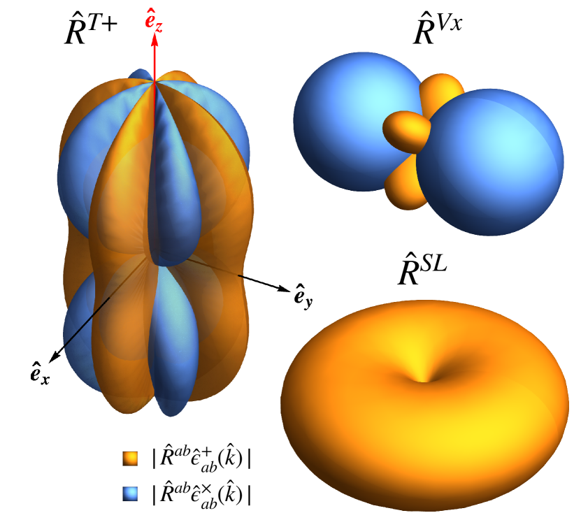
Figure 1: Antenna patterns $\displaystyle|\hat{R}^{ab}\hat{\epsilon}_{ab}^{A}(\hat{k})|$ depicted for three detector bases: $\displaystyle T+$ (left), $\displaystyle Vx$ (top-right), and $\displaystyle SL$ (bottom-right) for GW propagating from the directions $\displaystyle-\hat{k}$, with polarization $\displaystyle A=+$ (orange) and $\displaystyle A=\times$ (blue). The bases $\displaystyle T\times$ and $\displaystyle Vy$ correspond to those of $\displaystyle T+$ and $\displaystyle Vx$, respectively, but are rotated by $\displaystyle\pi/4$ and $\displaystyle\pi/2$ along the $\displaystyle\hat{e}_{z}$-axis.

III Generalized Hellings-Downs Correlations

A SGWB is an aggregate of GWs from various directions and with random phases, originating either cosmologically or astrophysically. The nanohertz SGWB was recently detected by PTAs, with a spectrum consistent with predictions from the inspiral of SMBHBs Agazie et al. (2023b). Stellar-mass compact binaries, including BHs and neutron stars, are expected to contribute to a similar background across frequencies ranging from $\displaystyle 10^{-4}$ Hz to $\displaystyle 10^{2}$ Hz, detectable by next-generation terrestrial and space laser interferometers, and long-baseline atom interferometers Abbott et al. (2016b, 2023); Banks et al. (2023).

Detection of the SGWB necessitates two-point correlations of the linear-response signals since the ensemble average of the strain vanishes. More explicitly, by expressing the strain tensor in terms of polarization tensors:

$$h_{ab}(f,\hat{k})=h_{+}(f,\hat{k})\,\hat{\epsilon}^{+}_{ab}(\hat{k})+h_{\times}(f,\hat{k})\,\hat{\epsilon}^{\times}_{ab}(\hat{k}),$$ (2)

the ensemble average $\displaystyle\langle\cdots\rangle$ results in $\displaystyle\langle h_{A}(f,\hat{k})\rangle=0$ and

$$\langle h_{A}(f,\hat{k})h^{*}_{A^{\prime}}(f^{\prime},\hat{k}^{\prime})\rangle=\frac{S_{h}(f)}{16\pi}\delta(f-f^{\prime})\delta_{AA^{\prime}}\delta^{2}(\hat{k},\hat{k}^{\prime}),$$ (3)

where $\displaystyle S_{h}(f)$ represents the power spectral density (PSD) of the SGWB, assumed to be isotropic.

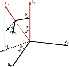
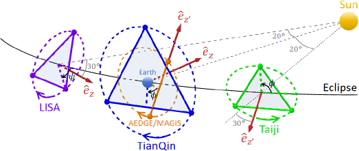
Figure 2: Left: Illustration of two frames with Cartesian coordinates $\displaystyle(\hat{e}_{x},\hat{e}_{y},\hat{e}_{z})$ and $\displaystyle(\hat{e}_{x^{\prime}},\hat{e}_{y^{\prime}},\hat{e}_{z^{\prime}})$, related through a rotation matrix defined by Euler angles $\displaystyle\Omega\equiv(\theta,\phi,\psi)$. $\displaystyle\theta$ represents the separation angle between $\displaystyle\hat{e}_{z}$ and $\displaystyle\hat{e}_{z^{\prime}}$, while $\displaystyle\phi$ and $\displaystyle\psi$ are the rotation angles about these respective axes. Right: Orbital and orientational configurations of the space missions considered: LISA-Taiji in heliocentric orbit and TianQin-AEDGE/MAGIS in Earth orbit. The normal vectors to the constellations for laser interferometers LISA, Taiji, and TianQin, as well as the baseline for the atom interferometer AEDGE/MAGIS, are represented by red arrows, denoted as $\displaystyle\hat{e}_{z}$ and $\displaystyle\hat{e}_{z^{\prime}}$. The LISA-Taiji pair rotates in opposite directions as viewed from the sun, with $\displaystyle\phi$ and $\displaystyle\psi$ increasing linearly due to self-rotation. The orbital planes of TianQin and AEDGE/MAGIS are assumed to be aligned, resulting in perpendicular $\displaystyle\hat{e}_{z}$ and $\displaystyle\hat{e}_{z^{\prime}}$ with $\displaystyle\phi$ modulating as the missions rotate.

A response channel of a detector at location $\displaystyle\vec{x}_{I}$, denoted by label $\displaystyle I$, receives both the GW signal ($\displaystyle s$) and noise ($\displaystyle n$), expressed as $\displaystyle{d}_{I}(f)={s}_{I}(f)+{n}_{I}(f)$, where the signal $\displaystyle{s}_{I}(f)$ accounts for GW contributions from all directions:

$$\displaystyle{s}_{I}(f)=\int{\rm d}^{2}\hat{k}\,R_{I}^{ab}(f)\,h_{ab}(f,\hat{k})\,\mathrm{e}^{-i2\pi f\hat{k}\cdot\vec{x}_{I}}.$$ (4)

The correlation between two response channels can be expressed as

$$\langle{d}_{I}(f){d}_{J}^{*}(f^{\prime})\rangle=\frac{1}{2}\left[S_{h}(f)\gamma_{IJ}(f)+\delta_{IJ}S_{n_{I}}(f)\right]\delta(f-f^{\prime}),$$ (5)

where the GW and noise are uncorrelated, and the noise is assumed to be Gaussian with PSD $\displaystyle S_{n_{I}}$. The ORF, $\displaystyle\gamma_{IJ}(f)$, is defined as Allen and Romano (1999):

$$\displaystyle\gamma_{IJ}(f) \displaystyle\equiv{R^{ab}_{I}R^{*cd}_{J}}\int\frac{{\rm d}^{2}\hat{k}}{{8\pi}}\sum_{A}\hat{\epsilon}^{A}_{ab}(\hat{k})\hat{\epsilon}^{A*}_{cd}(\hat{k})e^{i2\pi f\hat{k}\cdot(\vec{x}_{J}-\vec{x}_{I})}{}$$

$$\displaystyle\xrightarrow{|\vec{x}_{J}-\vec{x}_{I}|f\ll 1}\,\frac{2}{5}\mathrm{Tr}\left(R_{I}R_{J}^{\dagger}\right),$$ (6)

where the second line applies in the short-baseline limit, with the detector separation $\displaystyle|\vec{x}_{J}-\vec{x}_{I}|$ much smaller than the GW wavelength $\displaystyle 1/f$. For more general baselines, the ORF includes additional terms that involve contracting the response matrix with $\displaystyle\vec{x}_{J}-\vec{x}_{I}$ Flanagan (1993); Allen and Romano (1999).

Calculation of the ORF using the basis in Eq. (1) necessitates accounting for the relative orientation of the detector pair. This orientation can be parameterized by a rotation matrix $\displaystyle\mathcal{P}_{a}{}^{b}$, defined through three Euler angles $\displaystyle\Omega\equiv(\theta,\phi,\psi)$. As depicted in the left panel of Fig. 2, $\displaystyle\theta$ represents the separation angle between the $\displaystyle\hat{e}_{z}$-axes of the two detectors, while $\displaystyle\phi$ and $\displaystyle\psi$ serve as the rotation angles about each respective axis. An alternative representation utilizes the circular polarization basis: $\displaystyle\hat{R}^{\pm 2}\equiv(\hat{R}^{T+}\pm i\hat{R}^{T\times})/\sqrt{2},\hat{R}^{\pm 1}\equiv(\mp\hat{R}^{Vx}-i\hat{R}^{Vy})/\sqrt{2},\hat{R}^{0}=\hat{R}^{SL}$, resulting in the expression:

$$\gamma_{IJ}^{m_{I}m_{J}}=\frac{2}{5}\mathrm{Tr}\left(\hat{R}_{I}^{m_{I}}\mathcal{P}\hat{R}_{J}^{m_{J}\dagger}\mathcal{P}^{\dagger}\right)=\frac{2}{5}D^{j=2}_{m_{J},m_{I}}(-\psi,\theta,\phi),$$ (7)

where $\displaystyle D^{j=2}_{m_{I},m_{J}}$ is the spin-$\displaystyle 2$ Wigner D-matrix Wigner (1931), with its absolute value determined by $\displaystyle\theta$ and its complex phase determined by $\displaystyle\psi$ and $\displaystyle\phi$. For example, the correlation between two atom interferometers is proportional to $\displaystyle D^{2}_{00}=(1+3\cos 2\theta)/4$, which resembles the Hellings-Downs curve but without the redshift factor associated with PTAs. Additional details are provided in Supplemental Material.

Due to the stochastic nature of GWs, the ORF presented in Eq. (6) captures only the expected mean value of the correlation. For a Gaussian SGWB, the variance around this mean, termed the total variance, is expressed as Allen (2023); Bernardo and Ng (2022):

$$\Delta\gamma_{IJ}=\sqrt{\gamma_{II}\gamma_{JJ}+\gamma_{IJ}^{2}},$$ (8)

which also reflects the quadrupolar nature of the SGWB.

IV Identifying Quadrupolar Nature through Orbital Motion of Space Missions

The quadrupolar signature of the SGWB can be identified by scanning the ORFs across the configuration space defined by the Euler angles. Unlike PTAs or astrometric observation, which can utilize approximately $\displaystyle 10^{2}$ and $\displaystyle 10^{9}$ baselines respectively, terrestrial and space missions operating within the same frequency band currently, and foreseeably in the near future, have only a limited number of pairs available. However, the orbital motion and self-rotation of space missions enable an effective scan of the ORF within the configuration space, resulting in the modulation of correlations that reveal the quadrupolar nature of the SGWB. We consider two pairs of space missions, LISA-Taiji and TianQin-AEDGE/MAGIS, whose orbital and orientational configuration are shown in the right panel of Fig. 2. Correlations with terrestrial detectors in the same frequency band are similarly analyzed by considering the orbital and orientational configurations, with additional examples provided in Supplemental Material.

Both LISA and Taiji are in heliocentric orbits, with LISA trailing Earth by $\displaystyle 20^{\circ}$ and Taiji leading by the same margin. Their constellations are inclined at $\displaystyle 60^{\circ}$ relative to the ecliptic plane and rotate annually as they orbit the sun. From the sun’s perspective, the rotations of the two missions can be either aligned with identical inclination angles or opposed with inclination angles of different signs Joffre et al. (2021). Consequently, within the Euler angles defining their pair configuration, $\displaystyle\theta$ remains constant at approximately $\displaystyle 34^{\circ}$ or $\displaystyle 109^{\circ}$, respectively, while both $\displaystyle\psi$ and $\displaystyle\phi$ undergo linear changes with synchronized periodicity.

In the short-baseline limit where $\displaystyle f\ll 2.9\times 10^{-3}$ Hz, there are four possible correlations due to the two independent responses $\displaystyle\hat{R}^{T+}$ and $\displaystyle\hat{R}^{T\times}$ of each detector, for example:

$$\begin{split}\gamma_{IJ}^{++}&=\frac{1}{5}\left(D^{j=2}_{2,2}+D^{j=2}_{2,-2}+D^{j=2}_{-2,2}+D^{j=2}_{-2,-2}\right)\\ &=\frac{2}{5}\left[\cos 2(\phi-\psi)\cos^{4}\frac{\theta}{2}+\cos 2(\phi+\psi)\sin^{4}\frac{\theta}{2}\right].\end{split}$$ (9)

Correlations involving a switch from $\displaystyle+$ to $\displaystyle\times$ differ simply by shifting $\displaystyle\psi\rightarrow\psi+\pi/4$ or $\displaystyle\phi\rightarrow\phi+\pi/4$. Note that in the aligned constellation rotation configuration, the term $\displaystyle\cos^{4}(\theta/2)$ is two orders of magnitude greater than $\displaystyle\sin^{4}(\theta/2)$ due to the small $\displaystyle\theta(\approx 34^{\circ})$. This disparity causes the variation dependent on $\displaystyle\phi+\psi$ to be subleading compared to the static part involving $\displaystyle\phi-\psi$. Conversely, in the opposite rotation configuration where $\displaystyle\theta\approx 109^{\circ}$, observing variations becomes more effective. In the top panel of Fig. 3, we display the ORFs $\displaystyle\gamma_{IJ}^{++}$ (solid lines) along with their corresponding total variance (dashed lines) for both rotation configurations, clearly demonstrating that opposite rotations result in significantly larger modulations.

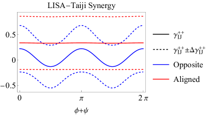
Figure 3: Top: The ORFs $\displaystyle\gamma_{IJ}^{++}$ for the LISA-Taiji pair (solid lines) and their corresponding total variances (dashed lines) are plotted against the varying Euler angle combination $\displaystyle\phi+\psi$ for both opposite (blue) and aligned (red) rotations viewed from the sun, with the static part $\displaystyle\phi-\psi$ set to $\displaystyle 0$. Significantly larger modulations are observed in the opposite rotation configuration compared to the aligned configuration. Similar trends for other ORFs, including $\displaystyle\gamma_{IJ}^{\times\times}$, $\displaystyle\gamma_{IJ}^{+\times}$ and $\displaystyle\gamma_{IJ}^{\times+}$, are shown in Supplemental Material. Bottom: The ORF $\displaystyle\gamma_{IJ}\propto\cos 2\phi$ for the TianQin-AEDGE/MAGIS pair (solid line) and its corresponding total variances (dashed lines) are depicted against the varying Euler angle $\displaystyle\phi$ for overlapping orbital planes with $\displaystyle\theta=\pi/2$. The channel for TianQin is selected as $\displaystyle T+$, whereas the ORF involving $\displaystyle T\times$, which is $\displaystyle\propto\sin 2\phi$, differs only by a phase shift of $\displaystyle\pi/2$. Both variables on the respective $\displaystyle x$-axes, $\displaystyle\phi+\psi$ and $\displaystyle\phi$, increase linearly over time.

In Earth orbit, TianQin comprises three satellites forming a triangle centered around Earth, while AEDGE/MAGIS consists of two satellites separated by $\displaystyle 138^{\circ}$ around the Earth Graham et al. (2017). As the $\displaystyle\hat{e}_{z}$-axis of the latter rotates within its orbital plane, both Euler angles $\displaystyle\theta$ and $\displaystyle\phi$ change over time. A simplified and optimal configuration involves aligning both orbital planes such that $\displaystyle\theta=\pi/2$ remains constant, and $\displaystyle\phi$ varies linearly, determined by the difference in the two orbital frequencies. In this configuration, the ORF involving the $\displaystyle T+$ channel of TianQin is given by $\displaystyle\gamma_{IJ}=\cos 2\phi\times\sqrt{3}/5$, as illustrated in the bottom panel of Fig. 3.

In practice, simultaneous observations between two missions can be divided into multiple time segments, each lasting $\displaystyle T_{\rm seg}$, significantly shorter than the variation timescale of the Euler angles. Within these segments, correlations between any two pairs of responses are established as per Eq. (5). Here, the quadrupolar information is embedded within the ORF matrix component $\displaystyle\gamma_{IJ}$, which varies between segments as $\displaystyle\Omega$ changes. For convenience, we define the normalized cross-correlated ORF as $\displaystyle\tilde{\gamma}_{IJ}\equiv(1-\delta_{IJ})\gamma_{IJ}/\sqrt{\gamma_{II}\gamma_{JJ}}$, and the PSD ratio, $\displaystyle\xi^{k}_{I}\equiv\gamma_{II}S_{h}^{k}/S_{n_{I}}^{k}$, at a given frequency bin $\displaystyle k$.

For detecting SGWB-induced power excess, the relevant measure is the signal-to-noise ratio (SNR) for the detector pair, which, in the weak signal limit ($\displaystyle\xi_{I}^{k}\ll 1$), is given by

$$\mathrm{SNR}^{2}_{k}\approx\frac{T}{T_{\rm seg}}\left(\sum_{I}(\xi_{I}^{k})^{2}+\sum_{I,J}\xi_{I}^{k}\xi_{J}^{k}\langle|\tilde{\gamma}_{IJ}|^{2}\rangle_{\Omega}\right),$$ (10)

at the $\displaystyle k$-th frequency of bin size $\displaystyle 1/T_{\rm seg}$. Here, $\displaystyle T$ is the total observation time, and $\displaystyle\langle\cdots\rangle_{\Omega}$ denotes the average over the Euler angle configurations across different segments. The ORFs between different channels within a single detector vanish due to the orthogonal basis.

In Eq. (10), only the last term within the bracket includes the quadrupolar information, while the first term arises from auto-correlations. A criterion for assessing the quadrupolar nature can be formulated using the log likelihood ratio ($\displaystyle\lambda_{\rm LR}$) between the full correlations and auto-correlations, as precisely captured by the last term of Eq. (10):

$$\langle\lambda_{\rm LR}^{k}\rangle\approx\frac{T}{T_{\rm seg}}\,\sum_{I,J}\xi_{I}^{k}\xi_{J}^{k}\langle|\tilde{\gamma}_{IJ}|^{2}\rangle_{\Omega}.$$ (11)

By comparing Eq. (10) with Eq. (11), it becomes evident that the time required to confirm the quadrupolar nature of the SGWB, $\displaystyle T_{Q}$, exceeds the duration necessary for the initial detection of a power excess, $\displaystyle T_{D}$. The ratio of the two durations is expressed as:

$$\frac{T_{Q}}{T_{D}}=1+\frac{\sum_{k^{\prime},L}(\xi_{L}^{k^{\prime}})^{2}}{\sum_{k,I,J}\xi_{I}^{k}\xi_{J}^{k}\langle|\tilde{\gamma}_{IJ}|^{2}\rangle_{\Omega}},$$ (12)

which depends on both the sensitivities of the detectors and their orbital configurations across different frequencies. Discussions for scenarios involving strong signal regions are included in Supplemental Material.

We attribute the source of the SGWB to compact binary populations, characterized by a spectrum $\displaystyle S_{h}(f)\equiv h_{c}(f)^{2}/f$ with $\displaystyle h_{c}=8.1\times 10^{-25}\times(f/\mathrm{Hz})^{-2/3}$ representing the characteristic strain Abbott et al. (2023), indicating weak signals for the four missions under consideration. For the LISA-Taiji pair, which exhibits similar sensitivities, the parameter $\displaystyle\xi_{I}^{k}$ is consistent across the four channels of the two detectors at a single frequency bin. Consequently, the duration required to identify quadrupolar patterns, according to Eq. (12), is a factor of $\displaystyle 1+4/\Sigma_{I,J}\langle|\tilde{\gamma}_{IJ}|^{2}\rangle_{\Omega}$ times longer than the initial discovery, approximating $\displaystyle 5.9$ after considering the orbital average $\displaystyle\langle|\tilde{\gamma}_{IJ}|^{2}\rangle_{\Omega}\approx 0.10$ in the short-baseline limit. However, when considering all relevant frequencies, the most sensitive bins occur when baseline is long compared to GW wavelength, which reduces the cross-correlations as discussed in Supplemental Material. The discovery of the SGWB power excess is estimated to require approximately $\displaystyle T_{D}\approx 0.083$ days, whereas the identification of its quadrupolar nature takes about $\displaystyle T_{Q}\approx 22$ days. These duration demand that $\displaystyle\Sigma_{k}\text{SNR}_{k}^{2}$ and $\displaystyle\Sigma_{k}\lambda_{\rm LR}^{k}$ reach $\displaystyle 2.71$, respectively, corresponding to a $\displaystyle 90\%$ confidence level. For the TianQin-AEDGE/MAGIS pair, the duration required extend to $\displaystyle T_{D}\approx 3.2$ days for initial detection and $\displaystyle T_{Q}\approx 42$ days for quadrupolar identification, respectively. The difference in these duration is primarily due to the distinct frequency sensitivities of the missions, in addition to orbital considerations. These discussions extend straightforwardly to space-terrestrial correlations by considering the variation in Euler angles.

V Discussion

Distinguishing the SGWB from noise involves characterizing its quadrupolar nature, evident in the cross-correlations between pairs of detectors. We systematically classify GW detectors based on antenna responses and construct the ORFs for detector pairs, which depends on the Euler angles relating the frames of the two detectors. We demonstrate this approach using several space missions as examples, showing how their relative orbital and orientational motions facilitate scanning of the ORFs through Euler angles, thereby identifying the quadrupolar nature of the SGWB. This approach underscores the enhanced capabilities of GW detector networks Klimenko et al. (2005); Ruan et al. (2021, 2020b); Zhang et al. (2021); Wang et al. (2022b); Orlando et al. (2021); Chen et al. (2021); Wang and Han (2021a); Wang et al. (2022c, 2021a); Wang and Han (2021b); Zhang et al. (2022); Cai et al. (2023); Jin et al. (2024); Li et al. (2023); Mentasti et al. (2024); Zhao and Wang (2024); Marriott-Best et al. (2024).

The time required to identify the quadrupolar nature is approximately one to two orders of magnitude longer than that needed for the initial discovery of a power excess. Specifically, we determine that the optimal configuration for the LISA-Taiji pair involves opposite rotations, which maximizes the variation in their relative configuration based on current orbital designs, thereby enhancing the detection of quadrupolar patterns.

Our discussion is not limited to space missions; it extends to a broader GW detector network that includes various tabletop high-frequency GW detectors Li et al. (2003); Arvanitaki and Geraci (2013); Berlin et al. (2022); Domcke et al. (2022); Berlin et al. (2023); Gao et al. (2024); Schmieden and Schott (2024); Alesini et al. (2023); Chen et al. (2023); Gao et al. (2023); Kahn et al. (2024); Navarro et al. (2024); Gatti et al. (2024); Valero et al. (2024); Domcke et al. (2024a); Schneemann et al. (2024); Domcke et al. (2024b), astrophysical observations Hui et al. (2013); Blas and Jenkins (2022a, b); Fedderke et al. (2022a, b); DeRocco and Dror (2023); Alves et al. (2024); Zwick et al. (2024); Lu et al. (2024); Crosta et al. (2024); Wang et al. (2024) and lunar-based detection Yan et al. (2024a); Ajith et al. (2024); Yan et al. (2024b) with diverse response functions. By integrating these systems into a unified network with optimized detector orientations and orbital configurations, we can significantly enhance the richness of the information gleaned from the detected signals.

Supplemental Material: Identifying the Quadrupolar Nature of Gravitational Wave Background through Space-based Missions

I Stochastic Gravitational Wave Detection via Detector Pairs

This section introduces a framework designed to explore how correlations between detector pairs can reveal the quadrupolar nature of the stochastic gravitational wave background (SGWB). Initially, we parameterize the SGWB, followed by introducing a generalized antenna pattern basis for gravitational wave (GW) detectors. Subsequently, we calculate their correlations. The section concludes with examples illustrating various detectors and their corresponding correlations.

I.1 Stochastic Gravitational Wave Background

Working within the transverse-traceless (TT) gauge for GWs and adopting the speed of light $\displaystyle c=1$ unit, GWs are modeled as perturbations of the spacetime metric. These perturbations can be represented as a superposition of plane waves emanating from direction $\displaystyle\hat{k}$ with frequency $\displaystyle f$:

$$h_{ab}(t,\vec{x})=\int_{-\infty}^{+\infty}{\rm d}f\int{\rm d}^{2}\hat{k}\,h_{ab}(f,\hat{k})\,\mathrm{e}^{\mathrm{i}2\pi f(t-\hat{k}\cdot\vec{x})}.$$ (S1)

Here, the Fourier coefficients $\displaystyle h_{ab}(f,\hat{k})$ represent the strain in the frequency domain and can be expanded based on GW polarizations:

$$h_{ab}(f,\hat{k})=h_{+}(f,\hat{k})\,\hat{\epsilon}^{+}_{ab}(\hat{k})+h_{\times}(f,\hat{k})\,\hat{\epsilon}^{\times}_{ab}(\hat{k}),$$ (S2)

where $\displaystyle h_{+}(f,\hat{k})$ and $\displaystyle h_{\times}(f,\hat{k})$ are the respective mode functions. The linear polarization basis tensors are defined as

$$\hat{\epsilon}^{+}_{ab}(\hat{k}) =\hat{l}_{a}\hat{l}_{b}-\hat{m}_{a}\hat{m}_{b},$$ (S3)

$$\hat{\epsilon}^{\times}_{ab}(\hat{k}) =\hat{l}_{a}\hat{m}_{b}+\hat{m}_{a}\hat{l}_{b},$$

where $\displaystyle\hat{l}$ and $\displaystyle\hat{m}$ are orthonormal vectors to $\displaystyle\hat{k}$, defined using the spherical angles $\displaystyle(\theta_{k},\phi_{k})$ as

$$\hat{k} \equiv\left(\sin\theta_{k}\cos\phi_{k},\sin\theta_{k}\sin\phi_{k},\cos\theta_{k}\right)^{T},$$ (S4)

$$\hat{l} \equiv\left(\cos\theta_{k}\cos\phi_{k},\cos\theta_{k}\sin\phi_{k},-\sin\theta_{k}\right)^{T},$$

$$\hat{m} \equiv\left(-\sin\phi_{k},\cos\phi_{k},0\right)^{T}.$$

The statistical properties of a Gaussian, stationary, unpolarized, and spatially homogeneous and isotropic SGWB are described by the first and second moments of the strain:

$$\langle h_{A}(f,\hat{k})\rangle=0,\qquad\langle h_{A}(f,\hat{k})h^{*}_{A^{\prime}}(f^{\prime},\hat{k}^{\prime})\rangle=\frac{S_{h}(f)}{16\pi}\delta(f-f^{\prime})\delta_{AA^{\prime}}\delta^{2}(\hat{k},\hat{k}^{\prime}),$$ (S5)

where $\displaystyle\langle\cdots\rangle$ denotes the ensemble average over the SGWB. $\displaystyle S_{h}(f)$ is the one-sided GW strain power spectral density (PSD), associated with the total energy density in GW as per the normalization Moore et al. (2015):

$$\rho_{\rm GW}=\int_{0}^{f_{\infty}}{\rm d}f\frac{\pi f^{2}}{4G}S_{h}(f),$$ (S6)

with $\displaystyle G$ representing the Newtonian constant.

I.2 Detector Responses

A GW detector typically responds linearly to GWs, converting them into signals. Representing the time series data by $\displaystyle d(t)$, its transformation into the frequency domain is given by:

$$d(f)=\int_{-\infty}^{\infty}{\rm d}t\,\mathrm{e}^{-2\pi ift}d(t)={s}(f)+{n}(f),$$ (S7)

where $\displaystyle s(f)$ and $\displaystyle n(f)$ denote the GW signal and measurement noise contributions, respectively. The signal component is formulated as:

$$\displaystyle{s}(f)=\int{\rm d}^{2}\hat{k}\,R^{ab}(f,\hat{k})\,h_{ab}(f,\hat{k})\,\mathrm{e}^{-i2\pi f\hat{k}\cdot\vec{x}}$$ (S8)

where $\displaystyle R^{ab}(f,\hat{k})$ is the response tensor of the detector located at $\displaystyle\vec{x}$. As the TT-gauge strain $\displaystyle h_{ab}$ is symmetric and traceless, only the symmetric and traceless components of $\displaystyle R^{ab}(f,\hat{k})$ contribute to detectable signals.

In the small-antenna limit, where the detector size is significantly smaller than the GW wavelength $\displaystyle 1/f$, the response tensor becomes independent of $\displaystyle\hat{k}$. A general traceless symmetric tensor $\displaystyle R^{ab}$ can be expanded in the following basis:

$$\displaystyle\hat{R}^{T+} \displaystyle=(\hat{e}_{x}\otimes\hat{e}_{x}-\hat{e}_{y}\otimes\hat{e}_{y})/\sqrt{2}, \displaystyle\hat{R}^{T\times} \displaystyle=(\hat{e}_{x}\otimes\hat{e}_{y}+\hat{e}_{y}\otimes\hat{e}_{x})/\sqrt{2},$$

$$\displaystyle\hat{R}^{Vx} \displaystyle=(\hat{e}_{x}\otimes\hat{e}_{z}+\hat{e}_{z}\otimes\hat{e}_{x})/\sqrt{2}, \displaystyle\hat{R}^{Vy} \displaystyle=(\hat{e}_{y}\otimes\hat{e}_{z}+\hat{e}_{z}\otimes\hat{e}_{y}))/\sqrt{2},$$

$$\displaystyle\hat{R}^{SL} \displaystyle=(\hat{e}_{z}\otimes\hat{e}_{z}-\mathbf{I}/3)\,\sqrt{3/2},$$ (S9)

aligned with the notation for GW polarization bases such as tensor-plus, tensor-cross, vector-$\displaystyle x$, vector-$\displaystyle y$, and scalar-longitudinal Will (1993), each normalized by $\displaystyle\mathrm{Tr}(\hat{R}^{A\dagger}\hat{R}^{B})=\delta^{AB}$. $\displaystyle\hat{e}_{x},\hat{e}_{y}$ and $\displaystyle\hat{e}_{z}$ are unit directional vectors of the Cartesian coordinate system, and $\displaystyle\mathbf{I}$ represents the $\displaystyle 3\times 3$ identity matrix. Linear combinations of the bases above yield the following circular bases $\displaystyle\hat{R}^{m}$, with $\displaystyle m$ denoting the azimuthal number:

$$\hat{R}^{0}=\hat{R}^{SL},\quad\hat{R}^{\pm 1}=\frac{1}{\sqrt{2}}(\mp\hat{R}^{Vx}-i\hat{R}^{Vy}),\quad\hat{R}^{\pm 2}=\frac{1}{\sqrt{2}}(\hat{R}^{T+}\pm i\hat{R}^{T\times}).$$ (S10)

Here, $\displaystyle\hat{R}^{m}$ also satisfies a similar normalization condition: $\displaystyle\mathrm{Tr}(\hat{R}^{m_{I}\dagger}\hat{R}^{m_{J}})=\delta^{m_{I}m_{J}}$.

I.3 Correlations and Overlap Reduction Functions

Within a network of detectors, each detector may have multiple response channels, each characterized by a basis as outlined in the previous subsection. The SGWB signal in any single channel is indistinguishable from uncalibrated measurement noise. However, correlations between pairs of channels can effectively distinguish between these two components, as encapsulated by the equation:

$$\langle d_{I}(f)d_{J}^{*}(f^{\prime})\rangle=\langle{s}_{I}(f){s}_{J}^{*}(f^{\prime})\rangle+\langle{n}_{I}(f){n}_{J}^{*}(f^{\prime})\rangle=\frac{1}{2}\left[S_{h}(f)\gamma_{IJ}(f)+\delta_{IJ}S_{n_{I}}(f)\right]\delta(f-f^{\prime}),$$ (S11)

where $\displaystyle I,J$ denote the response channels, with $\displaystyle I,J=1,2,\ldots,N_{\rm ch}$ for a total of $\displaystyle N_{\rm ch}$ channels. We assume that the SGWB and the measurement noise are uncorrelated, i.e., $\displaystyle\langle{s}_{I}(f){n}_{J}^{*}(f^{\prime})\rangle=\langle{n}_{I}(f){s}_{J}^{*}(f^{\prime})\rangle=0$, and that the noise is stationary, Gaussian, and uncorrelated between different channels:

$$\langle{n}_{I}(f){n}_{J}^{*}(f^{\prime})\rangle=\frac{1}{2}\delta(f-f^{\prime})\delta_{IJ}S_{n_{I}}(f).$$ (S12)

Here, $\displaystyle S_{n_{I}}(f)$ is the one-sided measurement noise power spectral density (PSD) of the $\displaystyle I$-th channel. The overlap reduction function (ORF), $\displaystyle\gamma_{IJ}(f)$, is defined as Allen and Romano (1999):

$$\displaystyle\gamma_{IJ}(f) \displaystyle\equiv R^{ab}_{I}R^{*cd}_{J}\int\frac{{\rm d}^{2}\hat{k}}{{8\pi}}\sum_{A}\hat{\epsilon}^{A}_{ab}(\hat{k})\hat{\epsilon}^{A*}_{cd}(\hat{k})\,\mathrm{e}^{i2\pi f\hat{k}\cdot(\vec{x}_{J}-\vec{x}_{I})}.$$ (S13)

Additionally, the variance of the correlated data $\displaystyle d_{I}(f)d_{J}^{*}(f)$ can be calculated as:

$$\langle|d_{I}(f)d_{J}^{*}(f)|^{2}\rangle-|\langle d_{I}(f)d_{J}^{*}(f)\rangle|^{2}=\frac{T^{2}}{4}\left[\left(\gamma_{II}(f)S_{h}(f)+S_{n,I}(f)\right)\left(\gamma_{JJ}(f)S_{h}(f)+S_{n,J}(f)\right)+\gamma_{IJ}^{2}(f)S_{h}^{2}(f)\right].$$ (S14)

In this expression, Eq. (S11) is applied to derive $\displaystyle\langle d_{I}(f)d_{J}^{*}(f)\rangle=\left[S_{h}(f)\gamma_{IJ}(f)+\delta_{IJ}S_{n_{I}}(f)\right]T/2$, where the delta function is replaced by the observation time $\displaystyle T$. Consequently, even in the strong signal limit where $\displaystyle S_{h}\gg S_{n,I/J}$, the stochastic nature of GWs introduces substantial variance in the correlated data, termed the total variance Allen (2023); Bernardo and Ng (2022):

$$\Delta\gamma_{IJ}=\left(\gamma_{II}\gamma_{JJ}+\gamma_{IJ}^{2}\right)^{1/2}.$$ (S15)

Defining the baseline vector $\displaystyle\vec{u}\equiv\vec{x}_{J}-\vec{x}_{I}$, with $\displaystyle u=|\vec{u}|$ and $\displaystyle\hat{u}=\vec{u}/u$, the general form of the ORF for symmetric and traceless response matrices can be simplified from Eq. (S13) as follows Flanagan (1993); Allen and Romano (1999):

$$\gamma_{IJ}=\rho_{1}(ku)R_{I}^{ab}R_{J}^{*ab}+\rho_{2}(ku)R_{I}^{ab}R_{J}^{*ac}\hat{u}^{b}\hat{u}^{c}+\rho_{3}(ku)R_{I}^{ab}R_{J}^{*cd}\hat{u}^{a}\hat{u}^{b}\hat{u}^{c}\hat{u}^{d},$$ (S16)

where $\displaystyle\rho_{1},\rho_{2}$ and $\displaystyle\rho_{3}$ are defined as linear combinations of spherical Bessel functions of the first kind $\displaystyle j_{n}(ku)$ Allen and Romano (1999):

$$\begin{bmatrix}\rho_{1}(ku)\\ \rho_{2}(ku)\\ \rho_{3}(ku)\end{bmatrix}\equiv\frac{1}{2(ku)^{2}}\begin{bmatrix}2(ku)^{2}&-4ku&2\\ -4(ku)^{2}&16ku&-20\\ (ku)^{2}&-10ku&35\end{bmatrix}\begin{bmatrix}j_{0}(ku)\\ j_{1}(ku)\\ j_{2}(ku)\end{bmatrix}.$$ (S17)

In the short baseline limit, where $\displaystyle u\ll 1/k$, the properties of the polarization basis tensors can be utilized:

$$\int\frac{{\rm d}^{2}\hat{k}}{{8\pi}}\sum_{A}\hat{\epsilon}^{A}_{ab}(\hat{k})\hat{\epsilon}^{A}_{cd}(\hat{k})=\frac{1}{5}(\delta_{ac}\delta_{bd}+\delta_{bc}\delta_{ad})-\frac{2}{15}\delta_{ab}\delta_{cd},$$ (S18)

to simplify the ORF as

$$\displaystyle\gamma_{IJ}=\frac{2}{5}R_{I}^{ab}R_{J}^{*ab}=\frac{2}{5}\mathrm{Tr}\left(R_{I}R_{J}^{\dagger}\right),$$ (S19)

under the assumption that the response matrix is symmetric and traceless.

Each response matrix for the channels can be expressed using the bases defined in Eq. (S9) or Eq. (S10) for each respective frame. The relative orientation between two detectors can be parameterized by a rotation matrix $\displaystyle\mathcal{P}_{a}{}^{b}(\Omega)$, which is defined using three Euler angles $\displaystyle\Omega\equiv(\theta,\phi,\psi)$:

$$\mathcal{P}(\Omega)=\mathcal{P}_{z}(-\phi)\mathcal{P}_{y}(\theta)\mathcal{P}_{z}(\psi)=\begin{pmatrix}\cos\phi&-\sin\phi&0\\ \sin\phi&\cos\phi&0\\ 0&0&1\end{pmatrix}\begin{pmatrix}\cos\theta&0&\sin\theta\\ 0&1&0\\ -\sin\theta&0&\cos\theta\end{pmatrix}\begin{pmatrix}\cos\psi&\sin\psi&0\\ -\sin\psi&\cos\psi&0\\ 0&0&1\end{pmatrix}.$$ (S20)

Under this transformation, the response matrix $\displaystyle R^{\prime}_{J}$, initially defined in its own Cartesian frame using axes $\displaystyle(\hat{e}_{x^{\prime}},\hat{e}_{y^{\prime}},\hat{e}_{z^{\prime}})$, transforms to $\displaystyle R_{J}=\mathcal{P}R^{\prime}_{J}\mathcal{P}^{\dagger}$ in the $\displaystyle I$-th detector’s frame with axes $\displaystyle(\hat{e}_{x},\hat{e}_{y},\hat{e}_{z})$. The configuration of Euler angles used in the rotation matrix is illustrated in the left panel of Fig. $\displaystyle 2$ in the main text.

Working in the circular polarization basis as defined in Eq. (S10), the angular correlation between two channels in their respective bases, $\displaystyle R_{I}=\hat{R}^{m_{I}}$ and $\displaystyle R^{\prime}_{J}=\hat{R}^{m_{J}}$, with their relative orientation described by $\displaystyle\mathcal{P}(\Omega)$, can be analytically determined as follows:

$$\gamma_{IJ}(\Omega)=\frac{2}{5}\mathrm{Tr}(\hat{R}^{m_{I}}\mathcal{P}\hat{R}^{m_{J}\dagger}\mathcal{P}^{\dagger})=\frac{2}{5}D^{j=2}_{m_{J},m_{I}}(-\psi,\theta,\phi).$$ (S21)

Here, $\displaystyle D^{j}_{m_{1},m_{2}}(-\psi,\theta,\phi)$ represents the Wigner D-matrix Wigner (1931), which quantifies the overlap between the modes $\displaystyle m_{I}$ and $\displaystyle m_{J}$ of the $\displaystyle j=2$ representation, as defined in their respective frames, which differ by the rotation $\displaystyle\mathcal{P}(\Omega)$.

The modulus of the Wigner D-matrix depends solely on $\displaystyle\theta$, while its phase is influenced by $\displaystyle\phi$ and $\displaystyle\psi$. More specifically, the azimuthal angles $\displaystyle\psi$ and $\displaystyle\phi$ contribute phase factors, expressed as $\displaystyle\mathcal{P}^{\dagger}_{z}(-\phi)\hat{R}^{m_{I}}\mathcal{P}_{z}(-\phi)=e^{im_{I}\phi}\hat{R}^{m_{I}}$ and $\displaystyle\mathcal{P}_{z}(\psi)\hat{R}^{m_{J}\dagger}\mathcal{P}^{\dagger}_{z}(\psi)=e^{-im_{J}\psi}\hat{R}^{m_{J}\dagger}$. Therefore, the Wigner D-functions can be formulated as:

$$\displaystyle D^{j}_{m_{1},m_{2}}(\psi,\theta,\phi)=\mathrm{e}^{i(m_{1}\psi+m_{2}\phi)}D^{j}_{m_{2},m_{1}}(0,\theta,0).$$ (S22)

The polar angle $\displaystyle\theta$ determines the amplitude as: $\displaystyle D^{j=2}_{m_{J},m_{I}}(0,\theta,0)=\mathrm{Tr}\left[\hat{R}^{m_{I}}\mathcal{P}_{y}(\theta)\hat{R}^{m_{J}\dagger}\mathcal{P}^{\dagger}_{y}(\theta)\right]$, resulting in six independent components with respect to the azimuthal numbers:

$$\displaystyle D^{j=2}_{0,0}(0,\theta,0) \displaystyle=\frac{1}{4}(1+3\cos{2\theta}),$$ (S23a)

$$\displaystyle D^{j=2}_{1,0}(0,\theta,0) \displaystyle=\sqrt{\frac{3}{2}}\cos\theta\sin{\theta},$$ (S23b)

$$\displaystyle D^{j=2}_{2,0}(0,\theta,0) \displaystyle=\frac{1}{2}\sqrt{\frac{3}{2}}\sin^{2}\theta,$$ (S23c)

$$\displaystyle D^{j=2}_{1,1}(0,\theta,0) \displaystyle=\frac{1}{2}(\cos{\theta}+\cos{2\theta}),$$ (S23d)

$$\displaystyle D^{j=2}_{2,1}(0,\theta,0) \displaystyle=\frac{1}{2}(1+\cos\theta)\sin\theta,$$ (S23e)

$$\displaystyle D^{j=2}_{2,2}(0,\theta,0) \displaystyle=\cos^{4}{\frac{\theta}{2}}.$$ (S23f)

Other components are related by the symmetries:

$$\displaystyle D^{j=2}_{m_{1},m_{2}}(0,\theta,0) \displaystyle=(-1)^{m_{1}+m_{2}}D^{j=2}_{m_{2},m_{1}}(0,\theta,0)=(-1)^{m_{1}+m_{2}}D^{j=2}_{-m_{1},-m_{2}}(0,\theta,0)$$ (S24)

$$\displaystyle=(-1)^{m_{2}}D^{j=2}_{m_{1},-m_{2}}(0,\theta-\pi,0)=(-1)^{m_{1}}D^{j=2}_{-m_{1},m_{2}}(0,\theta-\pi,0).$$ (S25)

II Statistics

This section outlines the analytical forecasts for detecting the SGWB and identifying its quadrupolar nature. Particularly, we analyze the timescales required for both discovery and quadrupolar identification.

Consider a network of GW detectors operating simultaneously, comprising $\displaystyle N_{\rm ch}$ channels with overlapping frequency windows. For a total observation period $\displaystyle T$, we divide it into multiple segments, each of equal duration $\displaystyle T_{\rm seg}$. This duration is considerably shorter compared to the timescale over which the detector configurations change. Within each segment, data are transformed into the frequency domain and labeled as $\displaystyle{d_{I}^{k,\alpha}}$, where the integers $\displaystyle I$, $\displaystyle k$, and $\displaystyle\alpha$ represent the channel, the frequency bin with central frequency $\displaystyle k/T_{\rm seg}$, and the segment index, respectively. Assuming that the noise in different channels is independent and Gaussian, the likelihood can be constructed in terms of the model parameters $\displaystyle\mathcal{O}$ as follows:

$$\mathcal{L}(\bm{d}\,|\mathcal{O})=\prod_{k,\alpha}\frac{1}{\mathrm{Det}\left[\pi C^{k,\alpha}(\mathcal{O})\right]}\exp\left\{-\sum_{I,J}d_{I}^{k,\alpha}\left[C^{k,\alpha}(\mathcal{O})\right]^{-1}_{IJ}(d_{J}^{k,\alpha})^{\dagger}\right\},$$ (S26)

where the covariance matrix is defined as:

$$\left[C^{k,\alpha}(\mathcal{O})\right]_{IJ}\equiv\frac{1}{2}\left[\delta_{IJ}S_{n_{I}}^{k}+\gamma_{IJ}(\Omega_{IJ}^{\alpha})S_{h}^{k}\right].$$ (S27)

Here, $\displaystyle S_{n_{I}}^{k}$ represents the noise PSD of channel $\displaystyle I$, and $\displaystyle S_{h}^{k}$ is the PSD of the SGWB. $\displaystyle\Omega_{IJ}^{\alpha}$ indicates the Euler angles describing the relative configuration between channels $\displaystyle I$ and $\displaystyle J$ for segment $\displaystyle\alpha$, and $\displaystyle\gamma_{IJ}(\Omega_{IJ}^{\alpha})$ is the corresponding ORF, as defined in Eq. (S13). The subsequent discussion will focus primarily on the ratio between the two terms in Eq. (S27), with the auto-correlation normalized to $\displaystyle\gamma_{II}=2/5$ and the noise PSD adjusted accordingly.

The capability of the detector network to estimate model parameters is quantified by the information matrix Fisher and Russell (1922):

$$\mathcal{I}_{ij}\equiv-\left\langle\frac{\partial^{2}\mathrm{ln}\,\mathcal{L}}{\partial\mathcal{O}_{i}\partial\mathcal{O}_{j}}\right\rangle\bigg{|}_{\mathcal{O}=\mathcal{O}_{\mathrm{truth}}},$$ (S28)

where $\displaystyle\mathcal{O}_{\mathrm{truth}}$ represents the true parameters. For any given model parameter $\displaystyle\mathcal{O}_{i}$, the variance of its estimator is expressed as:

$$\sigma^{2}_{i}\equiv(\mathcal{I})^{-1}_{ii},$$ (S29)

and the corresponding signal-to-noise ratio (SNR) is defined as:

$$\mathrm{SNR}^{2}_{i}\equiv\mathcal{O}^{2}_{i,\,\mathrm{truth}}/\sigma^{2}_{i}.$$ (S30)

We consider $\displaystyle\ln S_{h}^{k}$ as the model parameter. Dimensionless ORFs $\displaystyle\tilde{\gamma}_{IJ}\equiv(1-\delta_{IJ})\gamma_{IJ}/\sqrt{\gamma_{II}\gamma_{JJ}}$ are introduced to characterize the attenuation of cross-correlation relative to auto-correlation, and $\displaystyle\xi^{k}_{I}\equiv\gamma_{II}S_{h}^{k}/S_{n_{I}}^{k}$ denotes the PSD ratio between signal and noise from auto-correlation. Consequently, the SNR for a given frequency bin, denoted by $\displaystyle\mathrm{SNR}_{k}^{2}$, simplifies to:

$$\mathrm{SNR}^{2}_{k} \approx\begin{cases}\frac{T}{T_{\rm seg}}\left(\sum_{I}(\xi_{I}^{k})^{2}+\sum_{I,J}\xi_{I}^{k}\xi_{J}^{k}\langle|\tilde{\gamma}_{IJ}|^{2}\rangle_{\Omega}\right),\qquad\xi_{I}^{k}\ll 1,\\ \frac{N_{\rm ch}\,T}{T_{\rm seg}},\qquad\xi_{I}^{k}\gg 1,\end{cases}$$ (S31)

for weak and strong signal limit, respectively, where $\displaystyle\langle\cdots\rangle_{\Omega}$ denotes average over the channel configurations due to relative orientations of Euler angles. In the SNR expressions, $\displaystyle T/T_{\rm seg}$ corresponds to the number of independent data samples. In the weak signal limit, each auto-correlation and cross-correlation contributes to one term inside the bracket of Eq. (S31), while in the strong signal limit each channel has universal contribution.

After detecting potential signals from the SGWB, it is crucial for a network of GW detectors to confirm the quadrupolar nature of these signals to distinguish them from noise. For this purpose, we consider the log-likelihood ratio:

$$\lambda_{\rm LR}\equiv 2\left[\ln\mathcal{L}(\bm{d}\,|\mathcal{O}_{\rm truth})-\ln\mathcal{L}_{\rm auto}(\bm{d}\,|\mathcal{O}_{\rm truth})\right],$$ (S32)

where $\displaystyle\mathcal{L}_{\rm auto}$ denotes the likelihood that includes only auto-correlations, akin to Eq. (S26) but with the covariance matrix modified to:

$$\left[C^{k,\alpha}_{\rm auto}(\mathcal{O})\right]_{IJ}\equiv\frac{1}{2}\delta_{IJ}\left(S_{n_{I}}^{k}+\gamma_{II}S_{h}^{k}\right).$$ (S33)

For any given frequency bin, the log-likelihood ratio simplifies to:

$$\langle\lambda_{\rm LR}^{k}\rangle \approx\begin{cases}\frac{T}{T_{\rm seg}}\sum_{I,J}\xi_{I}^{k}\xi_{J}^{k}\langle|\tilde{\gamma}_{IJ}|^{2}\rangle_{\Omega},\qquad\xi_{I}^{k}\ll 1,\\ -\frac{2\,T}{T_{\rm seg}}\langle\mathrm{ln}\,\mathrm{Det}\left[\mathbf{I}_{N_{\rm ch}}+\tilde{\gamma}\right]\rangle_{\Omega},\qquad\xi_{I}^{k}\gg 1,\end{cases}$$ (S34)

where $\displaystyle\tilde{\gamma}$ represents the $\displaystyle N_{\rm ch}\times N_{\rm ch}$ matrix comprised solely of the cross-correlation elements $\displaystyle\tilde{\gamma}_{IJ}$, and $\displaystyle\mathbf{I}_{N_{\rm ch}}$ is the identity matrix. Compared to the SNR presented in Eq. (S31), the log-likelihood ratio primarily accounts for contributions from cross-correlations, thereby serving as a criterion for assessing the quadrupolar nature of the signal.

We compare the duration required for the initial discovery of a power excess due to the SGWB and the subsequent identification of its quadrupolar nature. Consider a power-law SGWB spectrum defined as $\displaystyle S_{h}(f)=A_{\rm GW}^{2}(f/f_{0})^{2\gamma}/f$, where $\displaystyle A_{\rm GW}$ represents the strain amplitude, $\displaystyle f_{0}$ is a reference frequency, and $\displaystyle\gamma$ describes the spectrum slope. We select $\displaystyle\ln A_{\rm GW}$ as the model parameter for calculating the SNR in Eq. (S30), assuming $\displaystyle\gamma$ as a fixed parameter. This yields an SNR summed over all frequencies, i.e., $\displaystyle\mathrm{SNR}^{2}=\Sigma_{k}\mathrm{SNR}^{2}_{k}$. The required duration for discovery, achieving a $\displaystyle 90\%$ confidence level, is then determined by $\displaystyle\mathrm{SNR}^{2}(T_{D})=2.71$.

Similarly, the log-likelihood ratio, as defined in Eq. (S32), sums over frequencies as $\displaystyle\langle\lambda_{\rm LR}\rangle\equiv\Sigma_{k}\langle\lambda_{\rm LR}^{k}\rangle$, with the threshold for quadrupolar identification required to meet $\displaystyle\langle\lambda_{\rm LR}(T_{Q})\rangle=\mathrm{SNR}^{2}(T_{D})$. By integrating Eq. (S31) and Eq. (S34) into the definitions for $\displaystyle T_{D}$ and $\displaystyle T_{Q}$, their ratio can be expressed as:

$$\frac{T_{Q}}{T_{D}}=\begin{cases}1+\frac{\sum_{k^{\prime},L}(\xi_{L}^{k^{\prime}})^{2}}{\sum_{k,I,J}\xi_{I}^{k}\xi_{J}^{k}\langle|\tilde{\gamma}_{IJ}|^{2}\rangle_{\Omega}},\qquad\xi_{I}^{k}\ll 1,\\ \vskip 5.0pt\cr-\frac{N_{\rm ch}}{2\,\langle\mathrm{ln}\,\mathrm{Det}\left[\mathbf{I}_{N_{\rm ch}}+\tilde{\gamma}\right]\rangle_{\Omega}},\qquad\xi_{I}^{k}\gg 1,\end{cases}$$ (S35)

where we consider all relevant frequencies to either fall within the weak signal limit or the strong signal limit.

III Examples

This section examines specific examples of laser and atom interferometers, focusing on space-based missions characterized by distinct orbital and orientation dynamics. Specifically, we consider two pairs of detectors: LISA-Taiji, which operates in heliocentric orbits, and TianQin-AEDGE/MAGIS, situated in Earth orbits. The results can be utilized to assess the capabilities of these systems for detecting the SGWB and identifying its quadrupolar nature. The benchmark SGWB we consider originates from compact binary populations, characterized by a spectrum $\displaystyle S_{h}(f)\equiv h_{c}(f)^{2}/f$, where $\displaystyle h_{c}=8.1\times 10^{-25}\times(f/\mathrm{Hz})^{-2/3}$ Abbott et al. (2023).

III.1 Laser Interferometers

Laser interferometers, such as LIGO and LISA, precisely measure GWs through the interference patterns of light beams. LIGO functions as an equal-arm Michelson interferometer, which splits a laser beam into two perpendicular paths. Each beam travels to a mirror, reflects back, and is then recombined to interfere with each other. Slight changes in the distance to one of the mirrors, caused by GWs, affect the phase relationship between the two beams, thereby altering the interference pattern. This effect is proportional to the contraction of both strain indices with the same distance vector. Assuming the arm directions as $\displaystyle\hat{e}_{x}$ and $\displaystyle\hat{e}_{y}$, the response matrix for LIGO is defined as:

$$R_{\rm LIGO}=\hat{R}^{T+}=\frac{1}{\sqrt{2}}(\hat{R}^{+2}+\hat{R}^{-2}).$$ (S36)

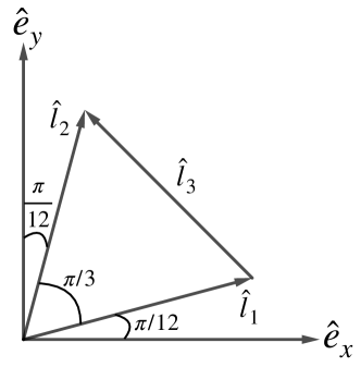
Figure S1: Configuration of a LISA-like GW detector constellation, depicting three spacecraft positioned at each vertex of an almost equilateral triangle. The unit directional vectors $\displaystyle\hat{l}_{i}$ represent the paths of the laser beams connecting the satellites. The $\displaystyle x-y$ coordinate system is chosen such that $\displaystyle\hat{l}_{i}=\cos\gamma_{i}\hat{e}_{x}+\sin\gamma_{i}\hat{e}_{y}$, where $\displaystyle i=1,2,3$ and $\displaystyle\gamma_{i}=\pi/12+(i-1)\pi/3$. The constellation features two independent response channels with response matrices $\displaystyle\hat{R}^{T+}$ and $\displaystyle\hat{R}^{T\times}$.

A LISA-like space-based detector comprises three satellites positioned at each vertex of an almost equilateral triangle. Each satellite houses two free-falling test masses, sending and receiving light to and from the nearby satellites, thus forming an interference pattern. By comparing the interference patterns of the two light paths, one can derive three combinations of response matrices: $\displaystyle X=\hat{l}_{1}\hat{l}_{1}-\hat{l}_{2}\hat{l}_{2},Y=\hat{l}_{2}\hat{l}_{2}-\hat{l}_{3}\hat{l}_{3},$ and $\displaystyle Z=\hat{l}_{3}\hat{l}_{3}-\hat{l}_{1}\hat{l}_{1}$, where $\displaystyle\hat{l}_{i}$ represents the unit directional vectors of the three beams, as illustrated in Fig. S1. In the center of mass frame of the triangle, defining $\displaystyle\hat{e}_{x}$ and $\displaystyle\hat{e}_{y}$ allows $\displaystyle\hat{l}_{i}$ to be expressed as $\displaystyle\hat{l}_{i}=\cos\gamma_{i}\hat{e}_{x}+\sin\gamma_{i}\hat{e}_{y}$, where $\displaystyle i=1,2,3$ and $\displaystyle\gamma_{i}=\pi/12+(i-1)\pi/3$. This definition aligns $\displaystyle X$ with LIGO’s response matrix in Eq. (S36) scaled by a factor of $\displaystyle{\sqrt{3}}/{4}$. Since only two of the three channels are independent, we can reconfigure the Michelson combinations $\displaystyle X$, $\displaystyle Y$, and $\displaystyle Z$ into three optimal combinations $\displaystyle A$, $\displaystyle E$, and $\displaystyle T$ Prince et al. (2002); Gair et al. (2013):

$$\displaystyle A \displaystyle=\frac{2}{3}(Y-Z)=\hat{R}^{T+}=\frac{1}{\sqrt{2}}(\hat{R}^{+2}+\hat{R}^{-2}),$$ (S37)

$$\displaystyle E \displaystyle=\frac{2}{3\sqrt{3}}(Y+Z-2X)=\hat{R}^{T\times}=\frac{1}{i\sqrt{2}}(\hat{R}^{+2}-\hat{R}^{-2}),$$ (S38)

$$\displaystyle T \displaystyle=\frac{1}{3}(X+Y+Z)=0.$$ (S39)

Here, the $\displaystyle A$ and $\displaystyle E$ channels can be treated as independent, while $\displaystyle T$ is a null channel insensitive to GW signals, useful for calibrating measurement noise.

We examine three space-based laser interferometer missions: LISA and Taiji, both operating in heliocentric orbits, and TianQin, which orbits the Earth. The orbital configurations of these missions are depicted in the right panel of Fig. $\displaystyle 2$ in the main text. LISA trails Earth by $\displaystyle 20^{\circ}$, and Taiji leads by the same margin, with arm lengths of $\displaystyle 2.5\times 10^{6}\,\mathrm{km}$ and $\displaystyle 3\times 10^{6}\,\mathrm{km}$, respectively. Both constellations are inclined at $\displaystyle 60^{\circ}$ relative to the ecliptic plane and complete an annual rotation as they orbit the sun. TianQin consists of three satellites orbiting Earth with an arm length of $\displaystyle L=\sqrt{3}\times 10^{5}\,\mathrm{km}$. Its orbital plane is strategically oriented to maintain continuous alignment with the reference binary pulsar source RX J0806.3+1527 Luo et al. (2016).

The main sources of noise in space-based laser interferometers stem from two categories: optical metrology system (OMS) noise, which includes shot noise, and acceleration noise related to the test masses Babak et al. (2021); Colpi et al. (2024). For LISA and Taiji, the corresponding PSDs, $\displaystyle S_{\mathrm{OMS}}(f)$ and $\displaystyle S_{\mathrm{acc}}(f)$, are expressed as Babak et al. (2021); Ren et al. (2023):

$$\begin{split}S_{\mathrm{OMS}}(f)=\ &(2\pi f)^{2}S_{x}\left[1+\left(\frac{2\,\rm{mHz}}{f}\right)^{4}\right],\\ S_{\mathrm{acc}}(f)=\ &\frac{S_{a}}{(2\pi f)^{2}}\left[1+\left(\frac{0.4\,\rm{mHz}}{f}\right)^{2}\right]\left[1+\left(\frac{f}{8\,\rm{mHz}}\right)^{4}\right].\end{split}$$ (S40)

The relevant parameters are:

LISA: $$\displaystyle S_{x}^{1/2}=15\times 10^{-12}\,\mathrm{m}\cdot\mathrm{Hz}^{-1/2},S_{a}^{1/2}=3\times 10^{-15}\,\mathrm{m}\cdot\mathrm{s}^{-2}\cdot\mathrm{Hz}^{-1/2},L=2.5\times 10^{6}\,\mathrm{km},$$ (S41)

Taiji: $$\displaystyle S_{x}^{1/2}=8\times 10^{-12}\,\mathrm{m}\cdot\mathrm{Hz}^{-1/2},~{}\,S_{a}^{1/2}=3\times 10^{-15}\,\mathrm{m}\cdot\mathrm{s}^{-2}\cdot\mathrm{Hz}^{-1/2},L=3\times 10^{6}\,\mathrm{km}.$$ (S42)

The total noise PSD for one channel, whether $\displaystyle A/\hat{R}^{T+}$ or $\displaystyle E/\hat{R}^{T\times}$, is given by Babak et al. (2021):

$$S_{n}(f)=\frac{8}{3}\frac{S_{\mathrm{OMS}}(f)+(3+\cos 4\pi fL)S_{\mathrm{acc}}(f)}{(2\pi fL)^{2}}\left[1+0.6(2\pi fL)^{2}\right],$$ (S43)

where the factor $\displaystyle 8/3$ is introduced to normalize the auto-correlation to $\displaystyle\gamma_{II}=2/5$ as compared with the literature Babak et al. (2021), and the term $\displaystyle\left[1+0.6(2\pi fL)^{2}\right]$ accounts for the deviations from the small-antenna limit, as discussed in Refs. Babak et al. (2021); Lu et al. (2019). We consider a frequency range for the two between $\displaystyle 10^{-4}$ Hz and $\displaystyle 10^{-1}$ Hz, where acceleration noise dominates at frequencies below $\displaystyle 10^{-3}$ Hz and OMS noise at higher frequencies.

For TianQin, the noise PSD can be approximated as Luo et al. (2016):

$$S_{n}(f)=\frac{8}{3}\frac{1}{L^{2}}\left[S_{x}+\frac{(3+\cos 4\pi fL)S_{a}}{(2\pi f)^{4}}\left(1+\frac{10^{-4}\,\mathrm{Hz}}{f}\right)\right]\left[1+0.6(2\pi fL)^{2}\right],$$ (S44)

with

$$S_{x}^{1/2}=1\times 10^{-12}\,\mathrm{m}\cdot\mathrm{Hz}^{-1/2},S_{a}^{1/2}=1\times 10^{-15}\,\mathrm{m}\cdot\mathrm{s}^{-2}\cdot\mathrm{Hz}^{-1/2},L=1.7\times 10^{5}\,\mathrm{km}.$$ (S45)

Given the shorter arm length compared to LISA and Taiji, TianQin’s sensitive frequency range is slightly higher, spanning $\displaystyle 10^{-3}$ Hz to $\displaystyle 1$ Hz.

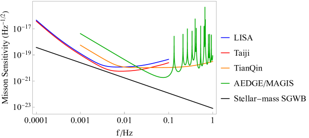
Figure S2: Mission sensitivity curves, $\displaystyle\sqrt{S_{n}/(N_{\rm ch}\gamma_{II})}$, for the four missions-LISA, Taiji, TianQin and AEDGE/MAGIS-are presented. The number of channels is $\displaystyle N_{\rm ch}=2$ for laser interferometers and $\displaystyle N_{\rm ch}=1$ for the atom interferometer, with the auto-correlation factor $\displaystyle\gamma_{II}=2/5$. The LISA-Taiji pair covers a sensitivity frequency range from $\displaystyle 10^{-4}$ Hz to $\displaystyle 10^{-1}$ Hz, whereas TianQin-AEDGE/MAGIS spans $\displaystyle 10^{-3}$ Hz to $\displaystyle 1$ Hz. The SGWB spectrum $\displaystyle\sqrt{S_{h}}$ from stellar-mass compact binary populations, characterized by $\displaystyle S_{h}(f)\equiv h_{c}(f)^{2}/f$, where $\displaystyle h_{c}=8.1\times 10^{-25}\times(f/\mathrm{Hz})^{-2/3}$ Abbott et al. (2023), is shown for comparison. This indicates that all four missions operate within the weak signal limit across their frequency ranges.

In Fig. S2, we present the mission sensitivities, represented as $\displaystyle\sqrt{S_{n}/(N_{\rm ch}\gamma_{II})}$, where $\displaystyle N_{\rm ch}=2$ for laser interferometers. For comparison, we also illustrate the benchmark SGWB spectrum, $\displaystyle\sqrt{S_{h}}$, which originates from compact binary populations Abbott et al. (2023).

III.2 Long-baseline Atom Interferometers

Atom interferometers harness a sequence of laser pulses to manipulate coherent ensembles of atoms, effectively splitting and then recombining their wave packets to generate interference patterns Dimopoulos et al. (2009, 2008). During operation, these atom wave packets traverse two distinct paths: one remains in the ground state, while the other is excited by the laser pulses. A phase difference accumulates between the two paths, influenced by both the arrival time of the laser pulses and the free-fall evolution of the atoms. This phase difference becomes sensitive to GWs passing through the setup. The GW-induced phase shift is directly proportional to the distances traveled by both the atoms and the laser pulses. Practically, expanding the space available for ultra-cold atom experiments is challenging. A viable approach is to implement a long laser baseline setup, where common laser pulses trigger two separate atom interferometers situated a significant distance apart. In such configurations, exemplified by space missions like AEDGE El-Neaj et al. (2020) and MAGIS Graham et al. (2017), the GW-induced phase shift is predominantly influenced by the laser’s travel path. Consequently, the GW response is largely determined by the projection of the strain tensor onto the baseline vector, resulting in a traceless response matrix:

$$R_{\rm AI}=\hat{R}^{SL}=\hat{R}^{0}=\sqrt{\frac{3}{2}}\left(\hat{e}_{z}\otimes\hat{e}_{z}-\frac{\mathbf{I}}{3}\right),$$ (S46)

where $\displaystyle\hat{e}_{z}$ represents the baseline direction.

The planned space missions AEDGE and MAGIS will operate in Earth orbit, featuring a single arm that spans $\displaystyle L=4.4\times 10^{4}\,\mathrm{km}$ and separates two satellites by $\displaystyle 138^{\circ}$ around the Earth Graham et al. (2017). The specific orbital plane for these missions has not yet been determined.

In long-baseline atom interferometers such as AEDGE and MAGIS, a single optical path exists, which avoids the acceleration noise typically associated with back-reaction from test masses. The predominant source of noise in these configurations is shot noise, inherent to the atom phase readout, denoted as $\displaystyle S_{\mathrm{atom}}$. This translates directly into the measurement noise for the system within the small-antenna limit Graham et al. (2016, 2017); Wang et al. (2021b):

$$S_{n}(f)=\frac{3}{2}\frac{S_{\mathrm{atom}}}{\frac{2f_{A}}{f}\frac{\sin(2\pi fQT_{\mathrm{int}})}{\cos(\pi fT_{\mathrm{int}})}\sin\left[\pi fT_{\mathrm{int}}-\pi f(N-1)L\right]\sin\left(\pi fNL\right)}.$$ (S47)

Here, $\displaystyle f_{A}$ is the atom transition frequency, $\displaystyle Q$ is the number of atom recombinations until the interferometry phase measurement, $\displaystyle N$ is the number of laser pulses used for exciting/de-exciting the atoms during one recombination period, and $\displaystyle T_{\mathrm{int}}$ is the duration of one recombination period. The additional factor $\displaystyle 3/2$ compared with the literature Graham et al. (2016, 2017); Wang et al. (2021b) is for normalization of the auto-correlation. For AEDGE/MAGIS, the parameters using ${}^{87}\mathrm{Sr}$ are as follows Graham et al. (2016, 2017):

$$S_{\mathrm{atom}}^{1/2}=10^{-5}\,\mathrm{Hz}^{-1/2},\ f_{A}=6.83\times 10^{13}\,\mathrm{Hz},\ Q=1,\ N=20,\ T_{\rm int}=7.5\,\textrm{s},\ L=4.4\times 10^{4}\,\mathrm{km}.$$ (S48)

The sensitive curve $\displaystyle\sqrt{S_{n}/(N_{\rm ch}\gamma_{II})}$, where $\displaystyle N_{\rm ch}=1$, is also shown in Fig. S2 to compare with laser interferometers and the benchmark SGWB, featuring a frequency range similar to TianQin.

III.3 LISA-Taiji Synergy

Each LISA-like detector features two independent channels, $\displaystyle A=\hat{R}^{T+}$ and $\displaystyle E=\hat{R}^{T\times}$. Consequently, there are four possible combinations of correlations between two detectors. In the short baseline limit, the ORFs parameterized by three Euler angles are given below

$$\displaystyle\tilde{\gamma}_{\rm{LT}}^{++} \displaystyle=2(D^{2}_{2,2}+D^{2}_{2,-2}+D^{2}_{-2,2}+D^{2}_{-2,-2})=\cos 2(\phi-\psi)\cos^{4}\frac{\theta}{2}+\cos 2(\phi+\psi)\sin^{4}\frac{\theta}{2},$$ (S49a)

$$\displaystyle\tilde{\gamma}_{\rm{LT}}^{\times\times} \displaystyle=2(D^{2}_{2,2}-D^{2}_{2,-2}-D^{2}_{-2,2}+D^{2}_{-2,-2})=\cos 2(\phi-\psi)\cos^{4}\frac{\theta}{2}-\cos 2(\phi+\psi)\sin^{4}\frac{\theta}{2},$$ (S49b)

$$\displaystyle\tilde{\gamma}_{\rm{LT}}^{+\times} \displaystyle=2i(D^{2}_{2,2}-D^{2}_{2,-2}+D^{2}_{-2,2}-D^{2}_{-2,-2})=\sin 2(\phi-\psi)\cos^{4}\frac{\theta}{2}-\sin 2(\phi+\psi)\sin^{4}\frac{\theta}{2},$$ (S49c)

$$\displaystyle\tilde{\gamma}_{\rm{LT}}^{\times+} \displaystyle=-2i(D^{2}_{2,2}+D^{2}_{2,-2}-D^{2}_{-2,2}-D^{2}_{-2,-2})=-\sin 2(\phi-\psi)\cos^{4}\frac{\theta}{2}-\sin 2(\phi+\psi)\sin^{4}\frac{\theta}{2},$$ (S49d)

where ‘L’ and ‘T’ refer to LISA and Taiji, respectively. The cross-correlation matrix for this pair is defined as follows:

$$\tilde{\gamma}=\begin{pmatrix}0&0&\tilde{\gamma}_{\mathrm{LT}}^{++}&\tilde{\gamma}_{\mathrm{LT}}^{+\times}\\ 0&0&\tilde{\gamma}_{\mathrm{LT}}^{\times+}&\tilde{\gamma}_{\mathrm{LT}}^{\times\times}\\ \tilde{\gamma}_{\mathrm{LT}}^{++}&\tilde{\gamma}_{\mathrm{LT}}^{+\times}&0&0\\ \tilde{\gamma}_{\mathrm{LT}}^{\times+}&\tilde{\gamma}_{\mathrm{LT}}^{\times\times}&0&0\end{pmatrix}.$$ (S50)

In heliocentric orbit, the normal vectors to the orbital planes of LISA and Taiji, corresponding to the $\displaystyle\hat{e}_{z}$ direction in their respective Cartesian frames, can be parameterized as:

$$\hat{n}_{\rm{L}}=\left(\sin\Theta_{\rm{L}}\cos\Phi_{\rm{L}},\sin\Theta_{\rm{L}}\sin\Phi_{\rm{L}},\cos\Theta_{\rm{L}}\right),\quad\hat{n}_{\rm{T}}=\left(\sin\Theta_{\rm{T}}\cos\Phi_{\rm{T}},\sin\Theta_{\rm{T}}\sin\Phi_{\rm{T}},\cos\Theta_{\rm{T}}\right),$$ (S51)

where $\displaystyle\Phi_{\rm{L}}=\Phi_{E}+20^{\circ}$ and $\displaystyle\Phi_{\rm{T}}=\Phi_{E}-20^{\circ}$ represent the angular positions of LISA and Taiji relative to Earth’s position $\displaystyle\Phi_{E}$. The inclination angle $\displaystyle\Theta_{\rm{L/T}}=\pm 60^{\circ}$ for LISA or Taiji has an undetermined sign. There are two potential configurations: aligned rotations with the same inclination signs, and opposite rotations with different inclination signs. Consequently, the Euler angle $\displaystyle\theta$, parameterizing the relative orientation between LISA and Taiji, remains constant:

$$\cos\theta=\hat{n}_{\rm{L}}\cdot\hat{n}_{\rm{T}}=\cos\Theta_{\rm{L}}\cos\Theta_{\rm{T}}+\cos 40^{\circ}\sin\Theta_{\rm{L}}\sin\Theta_{\rm{T}}=\frac{1}{4}(1\pm 3\cos 40^{\circ})\simeq 0.82\text{ or}\,-0.32,$$ (S52)

for aligned and opposite rotations, respectively.

The synchronous annual rotation of both missions contributes to a linear increase in the Euler angles $\displaystyle\phi$ and $\displaystyle\psi$ at the same frequency. As a result, the orbital configuration varies as $\displaystyle\phi+\psi$ increases, while $\displaystyle\phi-\psi$ depends on the initial configuration. The orbital average is thus calculated by integrating over $\displaystyle\phi+\psi$ while keeping $\displaystyle\phi-\psi$ constant, defined as: $\displaystyle\langle\cdots\rangle_{\Omega}=\textstyle\int_{0}^{2\pi}\!\cdots{\rm d}(\phi+\psi)/(2\pi)$, resulting in

$$\displaystyle\langle|\tilde{\gamma}^{++}_{\rm{LT}}|^{2}\rangle_{\Omega}=\langle|\tilde{\gamma}^{\times\times}_{\rm{LT}}|^{2}\rangle_{\Omega}=\frac{1}{2}\cos^{8}\frac{\theta}{2}\left(1+\tan^{8}\frac{\theta}{2}+\cos 4(\phi-\psi)\right),$$ (S53)

$$\displaystyle\langle|\tilde{\gamma}^{+\times}_{\rm{LT}}|^{2}\rangle_{\Omega}=\langle|\tilde{\gamma}^{\times+}_{\rm{LT}}|^{2}\rangle_{\Omega}=\frac{1}{2}\cos^{8}\frac{\theta}{2}\left(1+\tan^{8}\frac{\theta}{2}-\cos 4(\phi-\psi)\right).$$ (S54)

In the aligned rotation configuration, $\displaystyle\cos^{4}(\theta/2)$ is significantly larger than $\displaystyle\sin^{4}(\theta/2)$. This discrepancy results in the variation of ORFs dependent on $\displaystyle\phi+\psi$ being less pronounced compared to the static part controlled by $\displaystyle\phi-\psi$. Conversely, in the opposite rotation configuration, where $\displaystyle\sin^{4}(\theta/2)$ matches $\displaystyle\cos^{4}(\theta/2)$ in magnitude, variations become more apparent, as illustrated in the top panel of Fig. $\displaystyle 3$ in the main text and Fig. S3. We therefore adopt the opposite configuration with $\displaystyle\theta\approx 109^{\circ}$ for calculations and assume $\displaystyle\phi-\psi=0$ initially for simplicity.

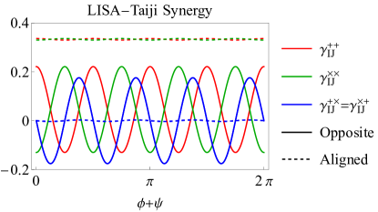
Figure S3: The four ORFs for the LISA-Taiji pair are depicted against the varying Euler angle combination $\displaystyle\phi+\psi$, for both opposite (solid lines) and aligned (dashed lines) rotations as viewed from the sun. The static component $\displaystyle\phi-\psi$ is set to $\displaystyle 0$. Notably, the opposite rotation configuration exhibits significantly larger modulations compared to the aligned configuration.

III.4 TianQin-AEDGE/MAGIS Synergy

For correlations between a space-based laser interferometer and an atom interferometer, three channels are available, yielding two possible correlations:

$$\displaystyle\tilde{\gamma}_{\rm T^{+}A} \displaystyle=\frac{1}{\sqrt{2}}(D^{2}_{2,0}+D^{2}_{-2,0})=\frac{\sqrt{3}}{2}\cos 2\phi\sin^{2}\theta,$$ (S55a)

$$\displaystyle\tilde{\gamma}_{\rm T^{\times}A} \displaystyle=\frac{1}{\sqrt{2}i}(D^{2}_{2,0}-D^{2}_{-2,0})=\frac{\sqrt{3}}{2}\sin 2\phi\sin^{2}\theta.$$ (S55b)

The corresponding cross-correlation matrix is then given by:

$$\tilde{\gamma}=\begin{pmatrix}0&0&\tilde{\gamma}_{\rm T^{+}A}\\ 0&0&\tilde{\gamma}_{\rm T^{\times}A}\\ \tilde{\gamma}_{\rm T^{+}A}^{*}&\tilde{\gamma}_{\rm T^{\times}A}^{*}&0\\ \end{pmatrix}.$$ (S56)

The relative orientation between TianQin and AEDGE/MAGIS is described by the separation angle $\displaystyle\Theta$ between their orbital plane normals, along with two rotation angles $\displaystyle\Phi=\Phi_{0}+{2\pi t}/{T_{\rm{T}}}$ and $\displaystyle\Psi=\Psi_{0}+{2\pi t}/{T_{\rm{A}}}$, which describe the orbital rotations of TianQin and AEDGE/MAGIS, respectively. These have orbital periods of $\displaystyle T_{\rm{T}}=3.15\times 10^{6}\,\mathrm{s}$ and $\displaystyle T_{\rm{A}}=3.7\times 10^{5}\,\mathrm{s}$. The Euler angles corresponding to these orbital dynamics are:

$$\theta=\arccos(-\sin\Theta\sin\Psi),\qquad\phi=\Phi+\arctan(\cos\Theta\cot\Psi).$$ (S57)

Consequently, the orbital average for this configuration is determined over $\displaystyle\Phi$ and $\displaystyle\Psi$, i.e., $\displaystyle\langle\cdots\rangle_{\Omega}=\textstyle\int_{0}^{2\pi}\int_{0}^{2\pi}\!\cdots{\rm d}\Phi{\rm d}\Psi/(2\pi)^{2}$, resulting in:

$$\langle|\tilde{\gamma}_{\mathrm{T^{+}A}}|^{2}\rangle_{\Omega}=\langle|\tilde{\gamma}_{\mathrm{T^{\times}A}}|^{2}\rangle_{\Omega}=\frac{3}{512}(41+20\cos 2\Theta+3\cos 4\Theta).$$ (S58)

As the orbit of AEDGE/MAGIS remains undetermined, we assume $\displaystyle\Theta=0$, corresponding to overlapping orbital planes, which maximizes the averaged ORF. In this setup, $\displaystyle\theta=\pi/2$ is constant, while $\displaystyle\phi=\pi/2+\Phi-\Psi$ changes with a period $\displaystyle T={T_{\rm A}T_{\rm T}}/({T_{\rm T}\mp T_{\rm A}})=4.2\times 10^{5}\,\mathrm{s}$ or $\displaystyle 3.3\times 10^{5}\,\mathrm{s}$ for aligned and opposite rotations, respectively. The rotation direction does not affect our analyses for SNR and quadrupolar identification, as both configurations yield the same averaged ORF. We depict the ORF and its intrinsic variance as functions of $\displaystyle\phi$ in the bottom of Fig. $\displaystyle 3$ in the main text. The orbital configurations are illustrated in the right panel of Fig. $\displaystyle 2$ in the main text.